The Economics of Renewable Energy Support

By Jan Abrell, Sebastian Rausch, and Clemens Streitberger∗

November 2018

This paper uses theoretical and numerical economic equilibriummodels to examine optimal renewable energy (RE) support policiesfor wind and solar resources in the presence of a carbon externalityassociated with the use of fossil fuels. We emphasize three mainissues for policy design: the heterogeneity of intermittent naturalresources, budget-neutral financing rules, and incentives for carbonmitigation. We find that differentiated subsidies for wind and solar,while being optimal, only yield negligible efficiency gains. Policieswith smart financing of RE subsidies which either relax budgetneutrality or use “polluter-pays-the-price” financing in the contextof budget-neutral schemes can, however, approximate socially opti-mal outcomes. Our analysis suggests that optimally designed REsupport policies do not necessarily have to be viewed as a costlysecond-best option when carbon pricing is unavailable. (JEL Q28,Q42, Q52, Q58, C61).

Decarbonization of energy systems to cope with the major challenges related tofossil fuels—limiting carbon dioxide (CO2) emissions to mitigate global climatechange, lowering local air pollution to yield health benefits, and enhancing the se-curity of energy supply—will require drastic changes in the future mix of energytechnologies in favor of using low-carbon, renewable energy (RE). Economistsseem to agree that carbon pricing is the most efficient regulatory strategy (Goul-der and Parry, 2008; Metcalf, 2009; Tietenberg, 2013), along with policies toaddress positive externalities related to technological innovation through R&Dinvestments and learning (Jaffe, Newell and Stavins, 2005; Acemoglu et al., 2012).Policies aimed at subsidizing the deployment of RE technologies are often consid-ered a costly second-best option failing to adequately reflect the heterogeneousmarginal social costs of multiple fossil-based and RE technologies. Moreover, bylowering the price of energy services, RE subsidies undermine incentives for en-ergy conservation (Holland, Hughes and Knittel, 2009). Yet, policies promotingclean energy from RE sources such as wind and solar are the most widely adopted

∗ Corresponding author: Sebastian Rausch, Department of Management, Technology and Economics,ETH Zurich, Switzerland, Center for Economic Research at ETH (CER-ETH), and MassachusettsInstitute of Technology, Joint Program on the Science and Policy of Global Change, USA (email:srausch@ethz.ch). Abrell (email: jabrell@ethz.ch) and Streitberger (email: clemenss@ethz.ch): Depart-ment of Management, Technology and Economics, ETH Zurich, Switzerland.We gratefully acknowledgefinancial support by the Swiss Competence Center for Energy Research, Competence Center for Researchin Energy, Society and Transition (SCCER-CREST) and Innosuisse (Swiss Innovation Agency).

1

2

form of actual low-carbon policy (Meckling, Sterner and Wagner, 2017).1This paper investigates how public policies aimed at supporting RE from wind

and solar should be best designed in the presence of a carbon externality related tothe use of non-renewable fossil fuels in energy supply and demand. An RE supportscheme comprises two essential elements: (1) subsidies paid to firms producingelectricity from RE and (2) a rule how these subsidies are financed. Examples ofwidely adopted forms for RE support include feed-in tariffs (FITs), guaranteeinga fixed output price per MWh of electricity sold, and market premiums whichessentially are output subsidies added to the wholesale electricity price. Theexpenses for a FIT or output subsidy paid to RE firms are typically financedthrough levying a tax on energy demand of consumers. RE quotas, renewable orclean portfolio standards are widely adopted examples of technology or intensitystandards which are blending constraints combining output subsidies for RE withinput production taxes to finance the RE support. A generic way of thinkingabout the design of RE support schemes is therefore to ask how RE subsidiesshould be structured and financed.

Our analysis emphasizes three major issues for RE policy design which areof relevance for the decarbonization of real-world energy systems. First, windand solar resources exhibit a large heterogeneity in terms of their temporal andspatial availability. Adding one MWh of solar electricity may thus yield verydifferent CO2 emissions reductions compared to adding one MWh of wind; theexact answer depends on the complex interactions between heterogeneous resourceavailability, time-varying energy demand, and the carbon-intensity and technologycosts of installed production capacities. We investigate how RE subsidies shouldbe structured to take into account these heterogeneous marginal external benefits.Second, most of the currently adopted forms of RE support are revenue-neutral,i.e. RE subsidies are financed through energy consumption taxes—either explicitly,as under a FIT or market premium approach, or implicitly, as for the case oftechnology or intensity standards. We analyze the implications of revenue-neutralRE support schemes in the context of optimal policy design. Third, in the absenceof stringent carbon pricing and given that RE support schemes are currentlythe most widely adopted form of actual low-carbon policies, a future world with“Janus-faced” energy systems—comprising either clean energy from RE sources orhighly carbon-intensive “dirty” fossil fuels (i.e., coal)—is not unlikely at all. WhileRE support policies induce investments in RE capacity and foster low-carbonenergy growth, it is ultimately cumulative emissions that count for addressingclimate change.2 We thus investigate how the financing of RE subsidies can be

1As of 2016, about 110 jurisdictions worldwide—at the national or sub-national level—had enactedpolicies subsidizing wind and solar power (REN, 2017). The Renewable Energy Directive by the EuropeanCommission (2010) established a policy framework for the promotion of RE in the EU with the aim tomeet by 2030 27% of total EU-wide energy consumption with renewables. In the United States, thefederal government provides sizable production and investment tax credits for RE and more than halfof the states have adopted renewable portfolio standards mandating minimum levels of RE generation(U.S. Department of Energy, 2016).

2Edenhofer et al. (2018) estimate that approximately 340 Gt CO2 emissions out of a global carbon

3

designed to provide incentives for carbon mitigation.To conceptualize and examine the fundamental economic principles for design-

ing RE support schemes for wind and solar power, we formulate theoretical andnumerical equilibrium models of optimal policy design where society (i.e., theregulator) is concerned with the management of an environmental externalityrelated to the use of fossil fuels. Decisions about energy supply and demandstem from profit- and utility-maximizing firms and consumers in the setting ofa decentralized market economy. We first theoretically characterize the optimalstructure and financing of RE subsidies as well as the conditions under whichsuch policies can implement socially optimal outcomes. To assess different REsupport schemes in an empirically plausible setting and to derive additional quan-titative insights, we develop a numerical framework which extends the theoreticalmodel and accommodates a number of features relevant for analyzing real-worldelectricity markets.3 While the model is calibrated with data for the Germanelectricity market, our numerical simulations yield qualitative insights germaneto the decarbonization of the electricity sector in many countries.

Our main findings can be summarized as follows. First, the optimal subsidyfor an RE technology reflects both the environmental and market value of theunderlying intermittent natural resource. The environmental value reflects theenvironmental damage avoided by replacing fossil-based with renewable energysupply. The market value reflects the economic rents for firms and consumerscreated by using intermittent resource. Accordingly, we find that the optimal REsubsidies for wind and solar differ. The quantitative analysis, however, suggeststhat the efficiency gains from differentiating RE subsidies across technologies arenegligible. Second, under an optimal RE support scheme, the revenues raisedfrom an energy demand tax exceed the expenses for RE subsidies. The importantimplication for policy design is that revenue-neutral support schemes, such as thewidely adopted FIT or RE quota policies, cannot implement a social optimum.We estimate that revenue-neutral RE support schemes entail large efficiency lossescompared to a first-best carbon pricing policy as they fail to appropriately incen-tivize the energy conservation channel. Third, we show that a RE support policycan implement the first-best outcome only if achieving the social optimum doesnot require a change in the fossil-based technology mix (relative to the unregu-lated market outcome). Fourth, the efficiency of RE support schemes importantlydepends on the way in which RE subsidies are financed. We find that combiningRE subsidies with an optimal tax on energy demand or using intensity or technol-ogy standards which link the financing of RE subsidies to the carbon intensity offossil-based energy suppliers are particularly effective ways for improving policy

budget of around 700 Gt CO2 (±275 Gt CO2)—consistent with having a “good chance” (i.e., 66%) ofkeeping global temperature below 2◦C as envisaged by the Paris agreement—would be consumed bycurrently existing, under construction, and planned coal power plants.

3These include, among others, hourly wholesale markets, multiple energy technologies, time-varyingand price-responsive demand, temporally and spatially heterogeneous quality of wind and solar resources,and output-dependent marginal cost and CO2 emissions to reflect flexibility and efficiency constraints atthe level of individual power plants.

4

design.Importantly, our analysis shows that—when carbon pricing is unavailable due

to political (and other) constraints—RE support policies do not necessarily haveto be viewed as a “costly” second-best option. Their ability to closely approximatesocially optimal outcomes crucially depends on (1) policy design, in particular howRE subsidies are financed, (2) market conditions (including the price responsive-ness of energy demand and the composition of fossil-based energy supply), and(3) the social valuation of environmental damages associated with carbon-basedenergy supply.

To the best of our knowledge, this paper is the first to investigate the optimaldesign of public policies to support intermittent RE resources in the presenceof a carbon externality. In light of the widespread use of RE policies to helpdecarbonize today’s energy systems, we thus believe that our analysis fills animportant gap in the existing literature. At a broader level, the paper contributesto the literature in public and environmental economics focused on understandingthe impacts and design choices of governmental regulation to address marketfailures and externalities related to pollution and technological progress throughlearning and R&D investments (see, for example, Fullerton and Heutel, 2005;Goulder and Parry, 2008; Fischer and Newell, 2008; Acemoglu et al., 2012). Whilemost studies have scrutinized various market-based and “command-and-control”approaches to carbon mitigation, the issue of how to best design public policiesto promote energy from intermittent RE resources has received surprisingly littleattention.

Recent empirical evidence (Kaffine, McBee and Lieskovsky, 2013; Cullen, 2013;Novan, 2015) has documented the temporal and spatial heterogeneity of intermit-tent wind and solar resources in terms of their environmental value, i.e. avoidedCO2 emissions per MWh of RE electricity. Based on an econometric ex-post as-sessment for Germany and Spain, Abrell, Kosch and Rausch (2017) find that theimpacts of RE support policies on wholesale electricity prices vary substantiallydepending on whether wind or solar energy is subsidized. While these papers gen-erally point out that the heterogeneous environmental and market values of differ-ent intermittent RE resources are not reflected in the prevailing policy incentivesthat guide investments in RE resources (Callaway, Fowlie and McCormick, 2017),the implications for policy design have not been analyzed. By typically adopting asimplified and aggregated representation of RE technologies, natural resource vari-ability, and time-varying energy demand, most of the work analyzing RE supportpolicies (Fischer and Newell, 2008; Rausch and Mowers, 2014; Kalkuhl, Edenhoferand Lessmann, 2015; Goulder, Hafstead and Williams, 2016) has abstracted fromthe fact that wind and solar resources are heterogeneous—thereby ignoring theidiosyncratic ways in which distinct intermittent RE resources interact with en-ergy supply and demand. Our framework investigates the optimal design of REsupport schemes in the context of multiple intermittent RE resources.

A small and recent literature has started to examine the effects of intermittent

5

energy sources for the provision of electricity employing the peak-load pricingmodel (Crew and Kleindorfer, 1976; Crew, Chitru and Kleindorfer, 1995). Am-bec and Crampes (2012) and Helm and Mier (2016) analyze the optimal andmarket-based mix of intermittent RE and conventional dispatchable energy tech-nologies. They do not, however, investigate the question of government supportfor RE resources. Ambec and Crampes (2017) theoretically examine optimal REpolicies in a setting with one intermittent RE resource, i.e. either wind or solar—thus not permitting to investigate the implications of multiple heterogeneous REresources for optimal policy design. Fell and Linn (2013) and Wibulpolprasert(2016) take into account the temporal and spatial resource heterogeneity, but fo-cus on comparing RE policies in terms of their cost-effectiveness to achieve a givenand exogenously determined emissions target. In contrast, our analysis explicitlyconsiders a carbon externality and analyzes optimal RE policy design when thechoice of environmental quality is endogenous.

The remainder of this paper is organized as follows. Section I presents ourtheoretical model and results. Section II describes the empirical quantitativeframework to investigate RE policies, including data sources and computationalstrategy. Section III presents and discusses our main simulation results.4 SectionIV reports on a number of robustness checks and model extensions. Section Vconcludes.

I. Theoretical Model and Results

A. Model setup

We have in mind a situation where society is concerned with the managementof an unpriced environmental externality that is related to the use of fossil fuelsin energy production. Although the reasoning below fits alternative applications,we let climate change and CO2 emissions abatement guide the modeling.5 Wefocus on the question how public policies supporting RE technologies should bebest designed to address the carbon externality.

ENERGY TECHNOLOGIES AND PRODUCTION.—–We consider a perfectly competitiveelectricity market in which in each period t, t′ ∈ {1, 2} electricity can be producedby conventional technologies (e.g., coal, gas, nuclear) and intermittent renewableenergy technologies (e.g., wind and solar). Output from different technologies is ahomogeneous good. Conventional technologies i ∈ {c, d} are assumed to be fullydispatchable, i.e. production can be varied freely at any point in time up to the

4An online appendix which documents the computer codes to replicate the quantitativeanalyses presented in the paper. All model files, including the data, can be downloadedat: https://www.ethz.ch/content/dam/ethz/special-interest/mtec/cer-eth/economics-energy-economics-dam/documents/people/srausch/Online Appendix TheEconomics of RenewableEnergySupport.zip.

5Our framework could be extended to also consider other externalities related to fossil fuel use suchas local air pollution and energy security considerations. We also abstract from explicitly representingexternalities related to the deployment of RE technologies such as fostering innovation, learning, andlocal employment effects.

6

installed capacity limit.6 Conventional technology i produces electricity output attime t, qit, incurring production cost Ci(qit) where C is a continuous and weaklyconvex function (C ′it := ∂Ci/∂qit ≥ 0 and C ′′it := ∂2Ci/∂q

2it > 0).7 CO2 emissions

associated with using technology i at time t depend on the level of output andare given by Ei(qit). For all i, we assume that the marginal emissions rate isstrictly positive (E′it := ∂Ei/∂qit > 0) and increases weakly in the level of output(E′′it := ∂2Ei/∂q

2it ≥ 0). Relative to the clean technology c, the dirty technology

d is characterized by a higher CO2 emissions rate (E′dt > E′ct). In addition, weassume that:

ASSUMPTION 1: In the absence of environmental policy, C ′ct(qct) > C ′dt(qdt),implying that the clean fossil-based technology c is not in the market.

While it would be straightforward to relax Assumption 1, it helps to focuson assessing the impacts of a supply-side driven fuel switch between high- andlow-carbon technologies in response to an RE policy. Our numerical analysis willscrutinize this assumption by modeling a number of (discrete) conventional energytechnologies which exhibit heterogeneous emissions intensities and are present inthe initial situation without RE support. Also, note that C ′ct(qct) > C ′dt(qdt)together with the convexity of cost functions implies that marginal cost functionsfor the clean and dirty conventional technology do not intersect.

We consider two RE technologies (e.g., wind and solar) which differ with respectto resource availability and investment cost for building production capacity. Out-put produced with either RE technology does not cause any CO2 emissions. Toreflect differences in resource availability, we index RE technologies by t and as-sume that:

ASSUMPTION 2: RE technology t is available in period t but not in period t′.

While in reality wind and solar resources are often available at the same time,Assumption 2 enables us to examine how RE support policies should be designedin light of heterogeneous RE resources. Our numerical analysis relaxes this as-sumption by incorporating data to characterize the empirical joint distribution ofwind and solar resources.

Without loss of generality, marginal generation cost for each RE technologyis normalized to zero. To produce output with RE technology t, it is requiredto install capacity kt, creating investment cost equal to Gt(kt). Investment costfunctions are strictly convex expressing the fact that investments first take placeat most productive sites (G′t := ∂Gt/∂kt > 0 and G′′t := ∂2Gt/∂k

2t > 0). As RE

technologies can produce output at zero marginal cost, output at time t is equal

6Note that conventional energy technologies can differ in terms of dispatchability, for example, dueto ramping constraints and maintenance. We abstract from such considerations here.

7The convex cost functions for conventional energy technologies should be viewed as an implicitrepresentation of multiple discrete suppliers with exogenously given production capacities ordered bymarginal cost.

7

to the installed capacity kt. Energy production from RE sources does not causeany emissions.

DEMAND AND ENERGY BALANCE.—–Consumers derive gross utility, St(dt), fromthe consumption of dt units of electricity at time t. With p(dt) denoting theinverse demand function, gross surplus at time t is St(dt) :=

∫ dt0 p(x)dx. St is a

continuous derivable function which we assume to be concave (S′t := ∂St/∂dt > 0and S′′t := ∂2St/∂d

2t ≤ 0).

We assume that energy demand only responds to price in the same period whichis equivalent to assuming that:ASSUMPTION 3: The cross-price elasticity of energy demand at time t withrespect to price at time t′ is zero, i.e. ∂dt/∂pt′ = 0,∀t.Assumption 3 considerably eases analytical complexity as it implies that St(dt)is separable across time periods. Importantly, this assumption does not rule outthe possibility that consumers increase or decrease demand in response to current-period changes in the electricity price.

Energy balance requires that at any point in time total energy production equalsenergy demand:

(1) kt +∑i

qit = dt .

ENVIRONMENTAL EXTERNALITY AND SOCIAL SURPLUS.—–The environmental exter-nality derives from CO2 emissions due to burning fossil fuels associated withsupplying energy from conventional technologies. CO2 as a uniformly-mixed pol-lutant is assumed to cause time-independent marginal damage equal to δ per unitof Ei(qit). δ may thus be viewed as the social cost of carbon (SCC) per ton ofemitted CO2.

The regulator is concerned with maximizing social surplus which is defined asgross utility net of private production cost associated with conventional and REsupply and the environmental damage to society caused by aggregate emissions:8

W :=∑t

[St(dt)−Gt(kt)−

∑i

Ci(qit)]

︸ ︷︷ ︸=Economic surplus

− δ∑t

∑i

Ei(qit)︸ ︷︷ ︸=Environmental

damage

.(2)

B. Social planner optimum

In the social optimum, the regulator chooses levels of output of conventionaland RE technologies (qit and kt) which maximize social surplus W subject to the

8We assume that environmental damage is additively separable from private consumption. Previousliterature (see, for example, Carbone and Smith, 2008) has highlighted the importance of taking intoaccount the non-separability between externalities and private utility for evaluating the effects of economicregulation. We leave this important extension for future research.

8

energy balance constraint (1) according to:

C ′it + δE′it ≥ S′t ∀t, i (qit)(3a)G′t = S′t ∀t (kt) .(3b)

The interpretation of the conditions for the social optimum is straightforward:energy produced by conventional technology i at time t (qit) is chosen such thatthe marginal social cost—comprising marginal private cost of production C ′it andthe marginal environmental damage δE′it—are equal to marginal private surplusS′t; energy produced with (or production capacity of) the RE technology t (kt) ischosen such that marginal private investment cost G′t and the marginal privatesurplus are equalized. The socially optimal pollution level is then given by E =∑i,tEi(qit).Depending on how strong the environmental motive (δ) is, energy production

from conventional technologies in the social optimum can take on two outcomes.If δ is “small”, then (C ′ct+δE′ct)/(C ′dt+δE′dt) > 1 implying that energy productionwith the clean technology is more costly and hence only the dirty technology isused. In contrast, for sufficiently high δ, only the clean conventional technology isused. To create a meaningful problem to examine RE support policies, we assumethat the social optimum involves a positive amount of energy supplied from REtechnologies at every t, i.e. kt > 0.9

C. The regulator’s problem in the decentralized economy

The fundamental problem of environmental regulation analyzed in this paperis to examine how RE support policies should be best designed to address thecarbon externality associated with fossil-based energy supply in a decentralizedmarket economy where equilibrium decisions about energy supply and demandstem from profit- and utility-maximizing firms and consumers (and can hence notbe directly controlled as in the social planner problem analyzed in Section I.B).

Hence, the regulator’s problem is to maximize social welfare W taking intoaccount a set of constraints that describe the equilibrium responses of economicagents with respect to market information (prices) and policy choice variables:

(4) maxb={st,τt,κit}

W (dt, kt, qit; δ)

9 If RE technologies are always more costly than conventional technologies (including the social costof carbon), i.e. G′t(kt) > min{C′ct(qct) + δE′ct(qct), C′dt(qdt) + δE′dt(qdt)}, ∀t, there is no role for REtechnologies in the social optimum and the fundamental problem of optimal RE policy support, whichmotivates our entire analysis, becomes trivial. By assuming that condition (3b) always holds as a strictequality, we rule out the case that energy supply in the social optimum is satisfied only with conventionalenergy production and that kt = 0.

9

s.t. (pt, dt, kt, qit) solve the market equilibrium conditions:

S′t = pt + τt ∀t (dt)(4a)C ′it + κit ≥ pt ∀t, i (qit)(4b)

G′t = ψt ∀t (kt)(4c)

ψt ={pt + st if output subsidy or intensity standardst if feed-in tariff

kt +∑i

qit = dt ∀t (pt)(4d)

where pt denotes the price of energy at time t.For given policy choice variables b, the equilibrium of the decentralized economy

is defined by prices and quantities {p∗t , d∗t , k∗t , q∗it} such that: (i) the marginalprivate utility from energy consumption equals the private marginal cost (4a), (ii)firms supplying energy with conventional technology i minimize cost of production(4b), (iii) firms supplying energy with RE technology t minimize cost (4c), and(iv) the wholesale energy markets clear (4d).10

POLICY INSTRUMENTS.—– Table 1 categorizes the different policy controls forpromoting RE supply contained in b along two key dimensions: the structure ofRE subsidies and the way RE subsidies are refinanced. RE producers can eitherreceive a guaranteed fixed price per MWh sold (ψt = st), as is the case under aFIT, or they can receive the subsidy on top of the market price, as is the caseunder a market premium approach (ψt = pt+ st). Moreover, RE subsidies can bedifferentiated in terms of the support for each RE technology (s1 6= s2) or theycan be uniform (s1 = s2).

Several ways of financing RE subsidy payments are conceivable. Under FIT andpremium systems the RE subsidies are often financed by levying a (time-constant)tax on energy demand (τ). In such a case, τ is endogenously determined by thefollowing revenue-neutrality constraint which has to be added to the upper-levelproblem in (4):

(5)∑t

τdt =∑t

stkt (τ) .

Alternatively, it is possible to view the (time-varying) energy demand tax (τt) asa distinct policy instrument chosen to optimally incentivize energy conservationvia the demand channel. In this case, the optimal policy involves choosing both(st, τt).

Yet another way of refinancing RE subsidies applies if intensity or technologystandards are used. Such standards are essentially blending constraints which

10Assuming perfect competition with free entry and exit and price-taking consumers, it is straightfor-ward to derive conditions (4a)–(4c) from the individual expenditure- and cost-minimization problems ofoptimizing consumers and firms, respectively.

10

Table 1. Taxonomy of policy designs which explicitly or implicitly promote RE supply.

Refinancing of RE subsidiesTax on energy Input taxes on energydemand (τt) production (κit)

No direct Carbon taxRE support Emissions trading

Structure oftechnology-neutral Guaranteed Feed-in tariff (FIT) Technology or intensity standards:or -differentiated output price

RE subsidies ·RE quota or renewable(st) portfolio standard (RPS)

Output Market premium ·Green offsetssubsidy

translate into implicit output subsidies for RE technologies (st) and implicit in-put taxes (κit) in energy production to finance RE subsidies (Holland, Hughesand Knittel, 2009). Consider the case of an RE quota which mandates that acertain share γ of total energy supplied has to come from RE sources—addingthe following constraint to the lower-level equilibrium problem in (4):

(6a)∑t

kt︸ ︷︷ ︸=Supply ofRE credits

≥ γ∑t

(kt +

∑i

qit

)︸ ︷︷ ︸

=Demand forRE credits

(pCredits) .

The RE quota can be conceived as a system of tradable credits where pCredits

corresponds to the post-trading equilibrium price of a credit determined by creditsupply and demand.11

A tradable RE standard is by definition revenue-neutral: expenses for RE sub-sidies are fully financed through implicit input taxes κit on energy producers.Output subsidies are paid to RE firms which receive one credit valued at pricepCredits for each MWh of electricity produced. From (6a) it then follows that theimplicit per-MWh tax under an RE quota is:

(6b) κRE quotait = γ pCredits .

The interpretation is that all energy firms have to hold γ credits for each MWhof energy produced. Because RE firms also receive one credit per MWh, theireffective net support per MWh of electricity produced is

(6c) sRE quota := pCredits − γpCredits = (1− γ)pCredits .

11We focus here on the case most relevant for real-world RE policy in which the standard does notdifferentiate between heterogeneous types of RE sources.

11

We propose and analyze a new design for a tradable and revenue-neutral inten-sity standard which links the amount of RE energy output to overall emissionsderived from using fossil fuels in energy production. We refer to such a scheme as“green offsets”. The main idea is that CO2 emissions have to be compensated oroffset by a certain amount of energy supplied from “green” (i.e., wind and solar)RE sources according to:

(7a)∑t

kt︸ ︷︷ ︸=Supply ofgreen offsets

≥ γ∑t

∑i

Eit(qit)︸ ︷︷ ︸=Demand forgreen offsets

(pCredits) .

γ here represents the “offset intensity”, i.e. the minimum amount of green energyrequired to offset overall CO2 emissions from “dirty” energy production, whichis chosen by the regulator. Here, pCredits indicates the value of a tradable “greenoffset” certificate. In an energy system where RE is relatively abundant, pCredits

is small; it is zero if all energy comes from green sources. If fossil fuels are stillthe dominant sources of energy supply, pCredits is large and provides an incentivefor RE producers to increase their supply.

Analogously to the case of an RE quota, the implicit input tax per MWh ofelectricity produced under a revenue-neutral “green offset” standard is:

(7b) κGreen offsetsit = γE′itp

Credits .

A green offset policy is thus an RE support scheme with “polluter-pays-the-price”refinancing: the expenses for RE subsidies are entirely refinanced by levyingproduction input taxes on fossil-based electricity firms which are proportional tothe carbon intensity. This implies that RE firms with zero emissions receive a netsupport equal to the credit price:

(7c) sGreen offsets := pCredits .

Under both forms of intensity standards, and compared to policies such as aFIT and market premium which directly choose the level of RE support, theonly policy choice variable of the regulator is the level of the intensity target γwhich then implicitly determines the RE subsidy rate s and refinancing taxes κitthrough (6a) and (6b) in the case of an RE quota and (7a) and (7b) in the caseof green offsets, respectively.

Finally, a carbon pricing policy—implemented through a CO2 tax or a systemof tradable emissions permits—can be represented as a specific input tax κi basedon the carbon content of energy production without direct support for RE (i.e.,st = 0). RE supply is, however, incentivized indirectly through lowering theproduction cost of RE technologies relative to fossil-based generation.

We now turn to characterizing optimal policies for RE support when the regu-lator can use different policy designs which draw on the instruments displayed in

12

Table 1. The second part of our theoretical analysis examines whether or not thevarious policy designs for RE support are optimal from a social perspective andcharacterizes the conditions under which RE policies can attain a social optimum.

D. Optimal policies for RE support

CARBON PRICING.—–We begin by analyzing a carbon pricing instrument whichcan be implemented equivalently either through a carbon tax or a system oftradable emissions permits. While carbon pricing does not explicitly subsidize REtechnologies, it establishes indirect support for RE by altering relative productioncost in favor of RE technologies. The case of a carbon tax constitutes a usefulbenchmark against which to compare RE support policies. It is straightforwardto show that:

PROPOSITION 1: The social optimum can be implemented by using for eachenergy firm i an input tax equal to its marginal environmental damage at time t(i.e., κit = δE′it, ∀i, t).

Proposition 1 simply recaps the standard result that the environmental external-ity can be fully internalized with a Pigouvian pricing rule which implements thesocial optimum by introducing a tax equal to the marginal environmental damage(Baumol, 1972; Metcalf, 2009). A carbon pricing instrument is efficient for tworeasons. First, it corrects the relative prices of energy technologies/fuels betweenfossil-based and RE technologies as well as between clean and dirty conventionaltechnologies. At the same time, it does not distort choices for investments in REtechnologies (i.e., wind vs. solar). Second, it corrects the price for energy servicesthereby incentivizing the optimal amount of energy conservation (i.e., the optimallevel of energy demand).

DIRECT RE SUPPORT SCHEMES.—–We now assume that carbon pricing or inputtaxes are not available, i.e. κit = 0, ∀i. How should the parameters of a direct REsupport scheme—comprising subsidies st for RE firms and refinancing taxes τtlevied on energy consumption—be chosen optimally? The following propositioncharacterizes the optimal policy:

PROPOSITION 2: The optimal RE support scheme consisting of RE subsidiesψ∗t—structured either as a feed-in tariff or a market premium—and an energydemand tax τ∗t , is given by:

ψ∗t = pt + δE′dtτ∗t = δE′dt .

PROOF: See Appendix A.A2. �The optimal RE policy support thus requires that, at the margin, consumers—

in addition to paying for the non-environmental cost of using resources to supplyenergy (pt)—bear the environmental damage associated with using fossil-based

13

energy (τ∗t = δE′dt).12 At the same time, RE supply is incentivized up to the pointwhere the marginal private costs are equal to the marginal benefits which reflectthe non-environmental and environmental value of the targeted RE resource.

An immediate implication of Proposition 2 is that:

COROLLARY 1: The optimal feed-in tariff and optimal market premium policylead to the same equilibrium allocation.

PROOF: Using the definition of ψ in (4c), Proposition 2 implies that the optimallevel of the FIT and market premium is given by, respectively:

s∗FITt = pt + δE′dt ∀t(8a)s∗Premiumt = δE′dt ∀t ,(8b)

and thus yields identical zero-profit conditions for RE production (4c) for the caseof a FIT and market premium. �

The welfare-maximizing RE subsidy rate per unit of energy produced from acertain RE resource therefore depends on two factors each affecting one of thetwo main components in social welfare W in equation (2). First, it depends onhow much the usage of the RE resource towards supplying energy contributesto the economic (non-environmental) surplus—this is reflected by its “marketvalue” expressed as unit revenues or the market price (pt). Second, it depends onthe environmental damage avoided by replacing conventional fossil-based energysupply with RE supply—this is reflected by its “environmental value” given byper-unit emissions rate of the (dirty) conventional technology valued at the socialcost of carbon (δE′dt).

If RE subsidies are structured such that firms directly receive the market in-come from supplying energy from the RE resource, as is the case under a marketpremium, the optimal RE subsidy does not need to explicitly reflect the marketvalue of the RE resource. Hence, pt does not appear in (8b) but instead showsup in zero-profit condition for RE production (4c). If RE firms are guaranteed afixed price, as is the case under a FIT, the optimal subsidy rate reflects both themarket and environmental value of the RE resource.

The optimal energy demand tax is equal for the FIT and market premium caseand reflects the marginal environmental cost caused in each period. By imposinga tax equal to δ, the regulator pushes demand towards the first-best level ofdemand. The tax is higher in periods with high emissions thus causing a largerdecrease in demand in high damage periods.

An important implication of (8b) is that the socially optimal FIT is higher forRE resources which are available in periods with high energy prices when demandis relatively large. In real-world systems, for example, electricity demand tends

12As we show below in Proposition 3, the clean conventional technology does not enter under (optimal)RE support policies, hence the marginal environmental damage is given by the marginal emissions rateof the dirty conventional technology, E′dt.

14

to peak around midday when solar resources are available. Following this lineof reasoning, the upshot of Proposition 2 is thus that the welfare-maximizingFITs should be higher for solar than for wind power. At the same time, however,the optimal RE subsidy in the case of a FIT or a market premium also dependson the environmental value of the RE resource that is promoted. Proposition 2also suggests that the RE subsidies should be higher for RE resources which areavailable in periods in which the marginal (price-setting) conventional technologyhas a high CO2 emissions intensity.

Proposition 2 thus implies that optimal RE subsidies should be differentiatedto reflect the market and environmental heterogeneity of the underlying resource(e.g., wind and solar). The heterogeneity of wind and solar energy resources is dueto differences in resource quality (how much is available?) and temporal availabil-ity (when is it available?) which, in turn, both interact with the characteristicsof energy demand (temporal variation) as well as conventional energy supply (in-stalled production capacity and carbon intensity of conventional producers).

NON-UNIFORMITY OF RE SUBSIDIES.—–The following corollary substantiates thepoint that optimal RE subsidies should be differentiated by type of RE resourceto reflect differences in the market and environmental value:COROLLARY 2: If either the social surplus function St is constant over timeor the emissions rate of the marginal energy producer does not vary with output(i.e., E′dt(qdt) = const.), then

(i) the optimal market premium (s∗Premiumt ) is uniform across RE technologies;

(ii) the optimal energy demand tax (τ∗t ) is uniform over time; and

(iii) if, in addition, marginal cost of the dirty technology does not vary withoutput (i.e., C ′′dt(qdt) = 0), the optimal FIT (s∗FITt ) is uniform across REtechnologies.

PROOF: See Appendix A.A3. �A constant social surplus function over time implies that energy demand does

not vary over time. Hence, the wholesale price and the marginal emissions rateare the same in every time period t. Under these circumstances, the optimal REsubsidies and energy demand taxes are uniform. The same result is obtained byassuming that the emissions rate of the marginal energy producer (i.e., the dirtyconventional technology) does not vary with output and, in addition for the case ofa FIT, that marginal costs of the marginal energy producer are constant in output.Given real-world characteristics of energy supply and demand, these conditionsare quite unlikely to hold in practice. First, conventional technologies exhibitsubstantial heterogeneity in terms of marginal costs, heat efficiencies, emissionsrates etc. Second, energy demand varies substantially over time reflecting dailyand seasonal fluctuations.

If RE resources were completely identical, then the optimal RE subsidies wouldbe uniform. In reality, however, the temporal availability of wind and solar re-sources differs. Heterogeneous RE resources interact with time-varying energy

15

demand and heterogeneous energy supply from conventional sources. Proposition2 simply expresses the fact that under these conditions pt and δE′dt in equations(8a) and (8b) are not independent of t. Thus, the optimal FIT or market premiumcannot be uniform across RE resource types. Similarly, the optimal tax on en-ergy demand is non-uniform across time in a way that reflects the heterogeneousenvironmental damage in each time period thus pushing the quantity demandedtowards the social optimum.

LINKING OF RE SUBSIDIES AND REFINANCING TAXES ON ENERGY DEMAND.—–In prac-tice, RE support schemes typically link RE subsidies and taxes on energy demand;for example, the level of the demand tax is often set in order to cover the expensespaid for RE subsidies. While Proposition 2 has characterized the optimal policyrules for RE subsidies and energy demand taxes, it does not shed light on howboth instruments should be linked to one another. In particular, is it optimal tochoose the energy demand tax such that is exactly yields the income needed tocover the expenses for the optimal RE subsidies? The following corollary showsthat an RE support scheme designed in this way cannot be optimal:

COROLLARY 3: Under an optimal RE support scheme {ψ∗t , τ∗t }, and if REfirms do not supply the entire market (i.e., kt < dt), the revenues raised from anenergy demand tax strictly exceed the expenses paid for RE subsidies.

PROOF: See Appendix A.A4. �Corollary 3 offers yet another perspective on the rules for optimal RE support

policies underlying Proposition 2. The optimal subsidy rate should, besides re-flecting the market value of the targeted RE resource (pt), subsidize RE supplyaccording to the marginal environmental value of the resource (δE′dt). Regard-less of whether the RE subsidy is structured as a FIT or a market premium, theoptimal energy demand tax to finance the RE subsidy is equal to this marginalenvironmental value, i.e. τ∗t = δE′dt. The intuition is that the market-value com-ponent of the optimal RE support does not have to be “re-financed”: in the caseof a market premium, RE producers directly receive the market value associatedwith RE production when selling into the market; in the case of a FIT, the marketvalue for social welfare is indirectly accounted for as the regulator sells the energybought from RE firms back into the market at the equilibrium wholesale price.

As long as RE production does not make up the whole market, the base for theenergy demand tax is larger than the one for RE subsidies, in turn implying thatthe net income (tax revenues - subsidy payments) for the regulator is positive.13

The important policy implication from Corollary 3 is therefore that energy de-mand taxes, which are typically used to refinance RE subsidies, should not bedetermined by considerations about revenue neutrality: requiring that the taxincome equals the payments for RE subsidies, implements a demand tax whichis too low. Energy demand and fossil-based energy generation then exceed their

13Also, note that the optimal tax and subsidy rates are quantity-based, i.e. per unit of physical energy(MWh) consumed or supplied.

16

respective optimal level leading to too little energy conservation and too highenvironmental damage.

E. Can RE support policies implement the social optimum?

Do optimal RE support schemes {ψ∗t , τ∗t }, comprising RE subsidies—either inthe form of a FIT or a market premium—and an energy demand tax, achieve thesocial optimum which, in the setting of a decentralized market economy, can beimplemented through carbon pricing (see Proposition 1)? And if so, what arethe conditions under which an optimal RE support policy can implement a socialoptimum?

To answer this question, we begin by building intuition on how well (optimal)RE policies can address the environmental externality through appropriately ex-ploiting the “fuel switch” channel for reducing pollution. Is a FIT, market pre-mium, or an energy demand tax capable of changing the relative size of dirty toclean conventional energy producers, i.e. induce a fuel switch?

PROPOSITION 3: With RE support through subsidies (ψt) or energy demandtaxes (τt), the clean fossil-based energy technology does not enter the market de-spite social concerns for the environmental externality.

PROOF: See Appendix A.A5. �The basic intuition behind Proposition 3 is that all instruments reduce the quan-

tity of energy supplied from conventional generation either by partially crowdingout conventional generation with increased supply from RE technologies (in thecase of FIT and market premium) or by reducing energy demand (in the case ofa demand tax). As (dirty) conventional energy generation is the marginal price-setting technology, the (wholesale) producer price of electricity declines. Thelower producer price implies that the profitability of sub-marginal energy pro-ducers using the clean conventional technology is reduced, too. As the cleanconventional energy producers are not in the market initially (i.e., before intro-ducing either one of the policy instruments), they have no incentive to enter themarket with these forms of policy support. This holds for both RE subsidies whichare uniform or differentiated across RE technologies as well as for a uniform ortime-specific energy demand tax.

Importantly, if one assumes that the clean conventional technology is initiallyin the market, the necessity of a fuel switch depends on which of the fossil-basedtechnology is the marginal generator. As long as the dirty conventional producersremain “price-setting”, no switch from dirty to clean fossil fuels is needed. If afuel switch is needed, the RE policies would need to achieve a re-ordering of themarginal cost of conventional technologies. This, however, is impossible as withthese instruments the regulator cannot directly affect the LHS of the zero-profitconditions for conventional producers (4b).14 The important implication from

14Without policies affecting directly the marginal cost of production, there exists the possibility that

17

Proposition 3 is thus that RE support schemes comprising a combination of REsubsidies, with either a FIT or market premium structure, and refinancing taxeson energy demand, fail to efficiently exploit the “fuel switch” channel.

Given Proposition 3, it is straightforward to characterize the condition underwhich an optimal RE support scheme can attain the first-best allocation in thesocial optimum:

PROPOSITION 4: The optimal RE support scheme consisting of RE subsidiesψ∗t—structured either as a feed-in tariff or a market premium—and an energydemand tax τ∗t implements the social optimum if and only if the clean fossil-basedenergy technology is not required to enter the market.

PROOF: See Appendix A.A6. �Intuitively, if the social optimum requires an energy supply mix which involves a

positive quantity of energy supplied from the clean fossil-based technology, an op-timal RE support scheme will fail to implement the first-best allocation.15 Table2 shows the four margins on which a socially optimal regulation of the environ-mental externality has to operate to efficiently exploit both the “fuel switch” and“energy conservation” channel. An optimal RE support scheme can only affectthree of these four margins in a direct manner. By subsidizing RE firms, anRE subsidy (FIT or market premium) can correct the relative prices of energysupplied from conventional vs. RE sources. By differentiating RE subsidies toreflect heterogeneity in the environmental value, it can correct the relative pricesof different types of RE resources (wind vs. solar). An energy demand tax candirectly stimulate the energy conservation channel. However, an RE subsidy, anenergy demand tax, or a combination of both, fails to correct the relative pricesof clean vs. dirty conventional energy production.

Proposition 4 also suggests that if the clean conventional technology plays noor only a minor role in the social optimum, an optimally designed RE supportscheme—taking into account the heterogeneous market and environmental valueof the targeted RE resources as well as incentivizing the correct amount of energyconservation (possibly through time-specific demand taxes)—can achieve or comeclose to the first-best allocation.

How close the optimal RE support policy comes to attaining the social optimumthus depends on the extent to which a fuel switch from dirty to clean conventionalenergy supply is required. This, in turn, depends on the characteristics of the

the policy-induced reduction in energy demand can affect the relative marginal cost of conventionalproducers. For this to occur, the marginal cost functions of conventional producers, C′it(qit), need tointersect and the demand reduction has to move production levels from the right to the left of theintersection point. Given empirically plausibly marginal cost functions for conventional, fossil-basedenergy technologies, such a case can be safely discarded as a mere theoretical possibility which seems tobe irrelevant for studying electricity supply under real-world conditions.

15If the clean fossil-based technology already supplied a positive quantity of energy in the unregulatedmarket equilibrium without concerns for environmental quality, the “no fuel-switch” condition underlyingProposition 4 can be re-stated. An optimal RE support then implements the social optimum if and only ifthe clean fossil-based energy technology is not required to expand its production relative to the unregulatedmarket equilibrium.

18

Table 2. Ability of different RE support policies to incentivize optimal abatement.

Can the policy correct...the relative prices of energy the price of

technologies/fuels? energyrenewables vs. within renewables: within fossil-based: services

fossil-based wind vs. solar low vs. high carbon (∆p ≶ 0)?

Single policy instrumentsCarbon pricing Y Y Y Y (p ↑↑)FIT or market premium

tech.-neutral Y N N N (p ↓)tech.-differentiated Y Y N N (p ↓)

Energy demand tax N N N Y (p ↑↑)

RE support schemes combining single instrumentsFIT or market premium with energy demand tax

revenue neutral Y Y/N N N (p ↑)optimal Y Y/N N Y (p ↑↑)

Intensity or technology standardsRE quota or RPS Y N N N (p ↑)Green offsets Y Y Y N (p ↑)

energy system at hand. For example, consider a system in which conventionalenergy supply capacities are given by natural gas and coal-fired plants only. If thegas price is “high”, only coal-fired plants are used in an unregulated equilibrium.An optimal environmental policy may then entail a fuel switch inducing coal-firedplants to be more costly than gas fired ones. In contrast, in a situation with “low”prices for natural gas, gas-fired plants may already be the cheaper technologyeven in the absence of environmental regulation. Adding social concerns aboutthe environmental externality will thus not induce a switch to more costly andcarbon-intensive coal-fired plants. Under such conditions, both an optimal REsupport scheme and a direct carbon pricing policy can achieve the social optimum.

TECHNOLOGY OR INTENSITY STANDARDS.—–RE support policies which are notefficient cannot implement a social optimum—even if achieving the socially opti-mal allocation does not require a fuel switch between dirty and clean fossil-basedgeneration. As intensity standards such as a green quota or green offset are byconstruction revenue-neutral and, thus, not efficient (see Corollary 3), they failto implement the social optimum.

PROPOSITION 5: An RE quota or a system of green offsets cannot achieve thesocial optimum.

PROOF: For the case of an RE quota, comparing conditions (3a) and (3b), whichcharacterize the first-best solution, with the zero-profit equilibrium conditions forRE producers (4b) and conventional producers (4c), and using the definitions forimplicit input taxes from (6b) and the implicit subsidy rate from (6c), yields,

19

respectively:

C ′it + δE′it = C ′it + γpCredits = S′t = pt ∀i, t(9)G′t = pt + (1− γ) pCredits = S′t = pt ∀t .(10)

From (10) it follows that pCredits = 0 which, however, contradicts (9) whichrequires that pCredits > 0 in order to efficiently internalize a positive marginalenvironmental damage δ > 0. The proof for the case of an intensity standard withgreen offsets proceeds analogously using instead (7b) and (7c) for the definitionsof implicit input taxes and subsidies. �

Proposition 5 bears out the important insight that technology or intensity stan-dards cannot reach a socially optimal allocation because the (implicit) subsidy toRE firms and the (implicit) input taxes on conventional energy producers are in-herently linked over the market for certificates—which in turn reflects the featurethat such policy schemes are revenue-neutral. If the quota price correctly reflectsthe marginal damage of emissions, the implied electricity price would correctlyreflect the social cost. At the same time, however, an efficient stimulation of REproduction requires that RE firms receive their market value plus an extra rentreflecting the marginal damage avoided (see Proposition 2). Thus, if the marginaldamage is already reflected in the market price, the RE support should be zero.This, however, is impossible as the quota price links the tax and the supportrate (i.e., the RE quota and system of green offsets are revenue-neutral). In fact,a quota price inducing an efficient tax level would imply that RE firms receive,on top of the subsidy rate, a too high market price resulting in over-investmentin RE capacity. Pushing too much RE with zero marginal cost into the marketwould in turn cause an inefficiently low electricity price undermining the incentivefor energy conservation. Thus, linking RE subsidies and refinancing taxes in arevenue-neutral manner and granting a subsidy on top of the wholesale electricityprice to RE firms makes it impossible to establish policy signals which induceefficient levels of both RE investments and RE generation.

Lastly, note that the failure of technology or intensity standards to implementthe social optimum does not depend on whether the RE support is differentiatedacross RE technologies to reflect the heterogeneity in the environmental value;rather, the inefficiency stems from the revenue-neutrality of such policy schemes.

II. Quantitative Empirical Framework

A. Overview

To assess alternative policy designs for RE support in an empirically plausiblesetting and to derive additional quantitative insights, we formulate a numericalmodel which extends our theoretical framework from Section I in a number of im-portant ways. First, we include multiple discrete conventional energy technologieswhich differ in terms of heat efficiency, carbon intensity, and installed production

20

capacities (thus relaxing Assumption 1). Importantly, this enables us to representthe market conditions for the German electricity market in the year 2014 and toassess policy-induced changes in the technology mix and supply side of the mar-ket with finer granularity. Second, we increase the temporal resolution at whichenergy supply and demand decisions are modelled, thus adding realism in termsof firms’ short-term production (generation dispatch) and long-term investmentdecisions as well as diurnal and seasonal variations in consumers’ energy use. Im-portantly, this enables us to characterize with fine granularity the empirical jointdistribution of wind and solar resources (thus relaxing Assumption 2).

The overall structure of the problem of optimal regulation remains identical:the regulator seeks to maximize social welfare W, including the valuation of envi-ronmental damage at social marginal cost δ, by choosing an RE support schemeb subject to market equilibrium conditions for energy supply and demand:

maxbW(p(b),x(b); δ)

s.t. p(b),x(b) ∈ A .(11)

A is the set of feasible allocations defined by equilibrium prices p(b) and quan-tities x(b) associated with energy generation and investments embodying firms’and consumers’ behavioral responses to policy choices b.

The remainder of this section describes our quantitative empirical frameworkincluding the derivation of the market equilibrium conditions which define A. Wealso provide detail on data sources, model calibration, and the computationalstrategy employed to solve the problem of optimal RE support policies.

B. Feasible equilibrium allocations A

Our characterization of the partial equilibrium model of electricity supply anddemand uses a complementarity-based formulation, i.e. a system of nonlinearinequalities with two classes of equilibrium conditions: zero-profit and market-clearing. Zero-profit and market-clearing conditions exhibit complementarity withrespect to quantities x and prices p, respectively.16 We now describe in detail thestructure and decision problems of economic agents to derive the conditions thatdefine A.17

PRODUCTION AND INVESTMENT.—–Electricity can be supplied from conventionaland renewable energy technologies. Different technologies are indexed by i ∈ Iwhere G ⊂ I contains RE technologies and B ⊂ I contains conventional (non-

16A characteristic of economic equilibrium models is that they can be cast as a complementarityproblem (Mathiesen, 1985; Rutherford, 1995), i.e. given a function F : Rn −→ Rn, find z ∈ Rn such thatF (z) ≥ 0, z ≥ 0, and zTF (z) = 0, or, in short-hand notation and using the “⊥” operator to indicatecomplementarity between equilibrium conditions and variables, F (z) ≥ 0 ⊥ z ≥ 0.

17While the structure of the quantitative model is largely identical to the one of the theoretical model,we introduce a self-contained notation for the numerical model. In particular, note that to reducenotational complexity, we redefine the technology index i in the quantitative model to include bothconventional and RE technologies.

21

renewable) technologies. Time (i.e., hours) is denoted by t ∈ T = {1, . . . , T}.Firms using technology i ∈ I choose quantities of investment Ii and energy outputXit in order to maximize total profits from selling electricity in wholesale marketst. Total profits Πi for energy producers using technology i are defined as:

Πi(Xi1, . . . , Xit, . . . , XiT , Ii) =∑t

[(πit − κit)Xit − cgi (Xit)]− ci

i(Ii) .(12)

πit denotes the wholesale price of electricity inclusive of any direct RE support.Conventional generators receive no RE support and sell their output at wholesalemarket price Pt at time t; RE firms receive a subsidy per MWh electricity sold(S) which can either take on the form of a FIT or a market premium which isconstant over the year:

πit =

Pt, if i ∈ BPt + ωiS, if i ∈ G and RE support with a market premiumωiS, if i ∈ G and RE support with a feed-in tariff.

ωi and κi are policy choice variables which can be controlled by the regulator butare viewed as given by firms. ωi implements a technology-specific differentiationof the RE support scheme; ωi = 1, ∀i, represents the case of uniform RE supportacross wind and solar technologies. κit is an input tax per MWh of electricitywhich can either represent an emissions tax or implicit taxes under an intensitystandard. cg

i (Xit) denote total generation cost associated with output, reflectingtechnology-specific heat efficiencies and fuel costs. For each technology categoryi, CO2 emissions Ei(Xit) are a function of the output level. While we modelelectricity generation at the technology level, we specify cg

i (Xit) and Ei(Xit) asquadratic functions to account for within-technology heterogeneity among indi-vidual electricity plants. Thus, the marginal cost and marginal emissions rate perMWh of electricity produced increase with output reflecting efficiency changes atthe plant level. ci

i(Ii) denote investment costs for installing capacity Ii.Profit-maximizing output and investment choices have to satisfy the following

constraint expressing that output at any time t cannot exceed available capacity:

αit(Ki + Ii

)≥ Xit ∀i, t(13)

where αit measures the availability of capacity which reflects the fact that con-ventional generators can be temporarily offline (due to, for example, maintenanceand outages) and that the production of renewable generators depends on weatherconditions. Ki denotes existing production capacities for each technology.

Maximizing (12) subject to (16) yields the following FOCs for optimal firm

22

behavior, which can be written in complementarity notation as follows:

∂cii(Ii)∂Ii

≥∑t

αitPIit ⊥ Ii ≥ 0 ∀i(14)

∂cgit(Xit)∂Xit

+ κi + P Iit ≥ πit ⊥ Xit ≥ 0 ∀i, t(15)

αit(Ki + Ii

)≥ Xit ⊥ P Iit ≥ 0 ∀i, t .(16)

P Ii is the shadow price of production capacity and is determined in equilibriumby (16). In equilibrium, Ii = 0 if the marginal cost of investment (∂cii(Ii)/∂Ii)exceeds marginal revenues for investment—condition (14) then holds with a strictinequality. A positive equilibrium level of investment results if marginal invest-ment cost equals marginal revenue which are given by the availability-weightedincome created by renting out production capacity at price P Iit. Similarly, a pos-itive quantity of energy is supplied at time t by using technology i if marginalcost of generation equals marginal revenue including RE subsidies—condition (15)then holds with equality.

DEMAND AND WHOLESALE ELECTRICITY PRICES.—–Electricity demand at time t,Dt(Pt, τt), is a function of the wholesale electricity price at time t (we thereforemaintain Assumption 3) and an energy demand tax τt ≥ 0. The market-clearingcondition for balancing energy supply and demand at time t determines the whole-sale electricity price at time t:∑

i

Xit = Dt(Pt, τt) ⊥ Pt “free” ∀t .(17)

Note that the we allow for the possibility of negative prices in situations where,for example, due to a high availability of RE sources, consumers have to becompensated for demanding a positive quantity of energy.

DEFINITION OF EQUILIBRIUM AND WELFARE.—–Given an RE support policy b ={ωi, S, τt, κi}, the set of feasible equilibrium allocations A is characterized by(i) prices p(b) = {P Iit, Pt} for production capacity and wholesale energy outputdetermined by market-clearing conditions (16) and (17) and (ii) quantities x(b) ={Xit, Ii} of energy outputs and investments into production capacity determinedby zero-profit conditions (14) and (15).

Analogously to the definition of social welfare in the theoretical model, welfarecomprises the economic surplus net of environmental damage:

(18) W =∑t

[∫ Dt

0Pt(x)dx−

∑i

(cii(Ii) + cg

it(Xit))]

︸ ︷︷ ︸=Economic surplus

− δ∑i,t

∫ Xit

0Ei(x)dx

︸ ︷︷ ︸=Environmental

damage

,

23

where Pt = D−1(Pt, τt) is the inverse demand function. Note that the definitionof the economic surplus also includes potential rents to the public sector due toexcess revenues earned from the regulation of the externality (for example, fromcarbon pricing or an RE support scheme where revenues of the refinancing taxexceed the expenses for RE subsidies).

CONSTRAINED-OPTIMAL RE SUPPORT SCHEMES.—–To represent real-world policiesfor RE support, we include additional constraints in the lower-level partial equi-librium problem which restrict the regulator’s choice of policy parameters b.

Under a FIT and market premium support scheme the expenses for RE subsidiesare fully covered by revenues generated with a time-independent energy demandtax τ which adjusts endogenously to ensure the following constraint is met:∑

t

τDt ≥∑i∈G

∑t

(πit − Pt)Xit ⊥ τ ≥ 0 .(19)

Under a revenue-neutral FIT or market premium support scheme the regulatorchooses b = {ωi, S} subject to the system of equilibrium constraints (14)–(17)and refinancing rules (19). Setting ωi = 1 would impose the additional constraintthat RE subsidies cannot be differentiated among RE technologies.18

Analogously to the conditions (6a) and (7a) for representing intensity standardsin the theoretical model, an intensity standard for RE relates the amount of“green” energy supplied in the economy (

∑i∈G,tXit) in a specific way to total

energy supply Ψ =∑i,tXit:∑i∈G,t

Xit ≥ γ F(Ψ) ⊥ S ≥ 0 ,(20)

where for the case of an RE quota and a system of green offsets F is given by,respectively:

F(Ψ) ={∑

i,tXit, if RE quota∑i,t

∫Xit0 Ei(x)dx, if Green offsets.

Under RE support through an intensity standard (RE quota or green offsets), theregulator chooses b = {γ} subject to the system of equilibrium constraints (14)–(17) and the intensity constraint (20) with the respective implicit input taxesgiven by: κRE quota

it = γS and κGreen offsetsit = γE′(Xit)S.

C. Computational strategy

The regulator’s problem of designing optimal RE support policies stated in (11)represents a Mathematical Program under Equilibrium Constraints (MPEC), i.e. abi-level optimization problem which maximizes an objective function subject to

18Note that ωiS corresponds to the policy choice variable st in the theoretical model in Section I.

24

a lower-level constraint set that contains an equilibrium problem (Luo, Pang andRalph, 1996). We cast the equilibrium problem in the lower-level part as a mixedcomplementarity problem (MCP) (Mathiesen, 1985; Rutherford, 1995) solvingfor primal and dual variables (i.e., quantities and prices). The advantage of thisapproach is that it naturally accommodates equilibria with corner solutions, forexample, zero technology-specific investments at a given point in time or non-binding capacity constraints in electricity production.

Owing to the lack of robust solvers (Luo, Pang and Ralph, 1996) for solvingMPECs, we reformulate the MPEC problem as a gridded MCP for which stan-dard solvers exist. Specifically, we use the MCP to perform a grid search overpolicy choice variables b using the PATH solver (Dirkse and Ferris, 1995) for com-plementarity problems and the General Algebraic Modeling System (GAMS).

D. Empirical specification

This section describes how we specify our quantitative model to be consistentwith year-2014 conditions of the German electricity market. The main idea isto construct an empirically plausible “no policy” reference case of the partialequilibrium model of German electricity supply and demand as described by thezero-profit and market-clearing equilibrium conditions (14)–(17). To cleanly inves-tigate the economic and environmental impacts of alternative policy designs forRE support, the “no policy” reference case assumes that market decisions aboutenergy supply and demand ignore the presence of the environmental external-ity, i.e. the equilibrium in the “no policy” benchmark represents an unregulatedmarket outcome.19

To bring our model to the data, we need to specify the following parameters andfunctions: resource availability of RE (wind and solar) resources over time (αit);cost and emissions functions for generation with technology i (cg

i and Ei); costfunctions for investments in production capacity for technology i (ci

i); installedproduction capacities for conventional energy technologies in the benchmark (Ki);and demand functions for energy at time t (Dt). We now describe in turn howthese functions and parameters are specified based on data.

TEMPORAL RESOLUTION AND AVAILABILITY OF RE RESOURCES.—–We model oneyear with hourly resolution to capture the temporal heterogeneity of RE supplyand interactions with hourly energy demand and supply (dispatch) decisions ofconventional energy producers. To reduce computational complexity, we selectT = 672 representative hours. Based on data for all hours of the year, we constructfor every season an average week. Each hour contained in an average week isobtained by averaging over the respective hour over all days belonging to thatseason.20

19For δ = 0, the regulator effectively maximizes market surplus (ignoring environmental damage) inwhich case the solution of the regulator’s problem in (4) coincides with the market outcome of the partialequilibrium model.

20In light of the concern that this procedure for selecting representative hours of the year may un-

25

To characterize the daily and seasonal variation of wind and solar resources, weuse hourly generation of wind and solar energy from the German transmission sys-tem operators (Amprion, 2018; Tennet, 2018; TransnetBW, 2018; 50Hertz, 2018).Hourly generation of hydro power is taken from the EnergyCharts (2015) pro-vided by the Fraunhofer Institute for Solar Energy Systems. To derive hourlyavailability profiles for wind and solar resources (αit), we assume that wind millsand solar panels would produce an energy output equal to their respective in-stalled production capacity. This enables us to calculate αit by relating observedhourly generation data for solar and wind to the maximally feasible energy outputgiven installed capacities. αit thus indicates the fraction of installed RE capacityavailable for production given the weather conditions that prevailed in 2014.

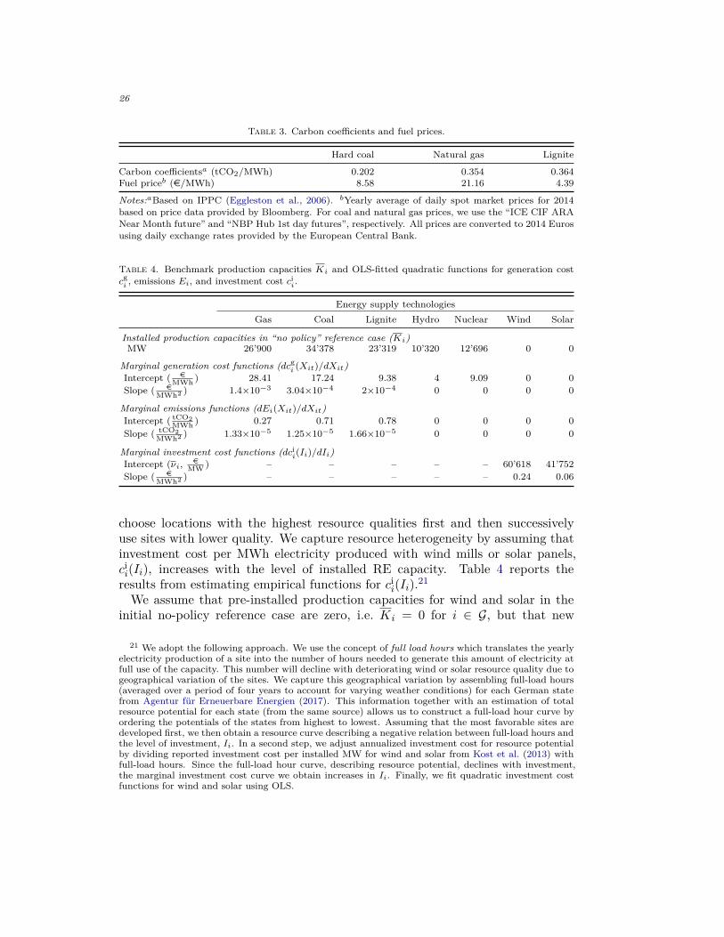
NON-RENEWABLE ENERGY TECHNOLOGIES.—–The technological options for supply-ing electricity from different non-renewable fuel sources (i ∈ B) are resolved at thetechnology level comprising lignite, hard coal, natural gas, nuclear, hydro, andothers (i.e., mainly biomass and some electricity generated from oil and waste).To take into account the heterogeneity of fossil-based and CO2-emitting plantsin terms of heat efficiencies and emissions intensity, we assume that generationcost functions cg

i (Xit) and emissions functions Ei(Xit) for lignite, hard coal, andnatural gas are quadratic in output. The corresponding functions for all othernon-renewable energy technologies are assumed to be linear.

To calibrate the functions cgi (Xit) and Ei(Xit), we first obtain plant-level heat

efficiencies for German power plants from Open Power System Data (2017). Sec-ond, we assemble data on fuel prices and emissions coefficients by fuel. For theformer, we take yearly averages of daily spot market prices for the year 2014 asprovided by Bloomberg. The latter are based on IPPC standard emissions coef-ficients (Eggleston et al., 2006) for each fuel. Table 3 shows the data for carboncoefficients and fuel prices. Third, we construct plant-level fuel costs and CO2emission rates by multiplying the heat efficiency for each plant with the respectivefuel price and emissions coefficient. Lastly, ordering all plants from low to highmarginal cost, we then use ordinary least squares (OLS) to estimate the interceptand slope coefficients of the marginal generation costs and emissions functions.Table 4 reports the estimated coefficients.

Installed generation capacities for conventional energy technologies Ki in 2014are taken from Open Power System Data (2017). We assume that conventionalenergy firms do not invest in new capacity (i.e., Ii = 0 for i ∈ B); production isthus restricted to what is feasible given pre-installed capacities.

INVESTMENT COSTS AND HETEROGENEOUS RESOURCE QUALITY.—–While the costsfor fossil fuels and emissions associated with energy supply from wind and solarare zero, i.e. cg

i (Xit) = Ei(Xit) = 0 for i ∈ G, the major cost incurred is the capitalcost for installing production capacity. At the same time, there is considerablespatial variation regarding the resource availability of wind and solar. Investors

intentionally smooth out hours with extremely low or high resource availability, Section IV reports onrobustness checks with respect to the number of hours.

26

Table 3. Carbon coefficients and fuel prices.

Hard coal Natural gas Lignite

Carbon coefficientsa (tCO2/MWh) 0.202 0.354 0.364Fuel priceb (e/MWh) 8.58 21.16 4.39

Notes:aBased on IPPC (Eggleston et al., 2006). bYearly average of daily spot market prices for 2014based on price data provided by Bloomberg. For coal and natural gas prices, we use the “ICE CIF ARANear Month future” and “NBP Hub 1st day futures”, respectively. All prices are converted to 2014 Eurosusing daily exchange rates provided by the European Central Bank.

Table 4. Benchmark production capacities Ki and OLS-fitted quadratic functions for generation costcgi , emissions Ei, and investment cost ci

i.

Energy supply technologiesGas Coal Lignite Hydro Nuclear Wind Solar

Installed production capacities in “no policy” reference case (Ki)MW 26’900 34’378 23’319 10’320 12’696 0 0

Marginal generation cost functions (dcgi (Xit)/dXit)

Intercept ( eMWh ) 28.41 17.24 9.38 4 9.09 0 0

Slope ( eMWh2 ) 1.4×10−3 3.04×10−4 2×10−4 0 0 0 0

Marginal emissions functions (dEi(Xit)/dXit)Intercept ( tCO2

MWh ) 0.27 0.71 0.78 0 0 0 0Slope ( tCO2

MWh2 ) 1.33×10−5 1.25×10−5 1.66×10−5 0 0 0 0

Marginal investment cost functions (dcii(Ii)/dIi)

Intercept (νi, eMW ) – – – – – 60’618 41’752

Slope ( eMWh2 ) – – – – – 0.24 0.06

choose locations with the highest resource qualities first and then successivelyuse sites with lower quality. We capture resource heterogeneity by assuming thatinvestment cost per MWh electricity produced with wind mills or solar panels,cii(Ii), increases with the level of installed RE capacity. Table 4 reports the

results from estimating empirical functions for cii(Ii).21

We assume that pre-installed production capacities for wind and solar in theinitial no-policy reference case are zero, i.e. Ki = 0 for i ∈ G, but that new

21 We adopt the following approach. We use the concept of full load hours which translates the yearlyelectricity production of a site into the number of hours needed to generate this amount of electricity atfull use of the capacity. This number will decline with deteriorating wind or solar resource quality due togeographical variation of the sites. We capture this geographical variation by assembling full-load hours(averaged over a period of four years to account for varying weather conditions) for each German statefrom Agentur fur Erneuerbare Energien (2017). This information together with an estimation of totalresource potential for each state (from the same source) allows us to construct a full-load hour curve byordering the potentials of the states from highest to lowest. Assuming that the most favorable sites aredeveloped first, we then obtain a resource curve describing a negative relation between full-load hours andthe level of investment, Ii. In a second step, we adjust annualized investment cost for resource potentialby dividing reported investment cost per installed MW for wind and solar from Kost et al. (2013) withfull-load hours. Since the full-load hour curve, describing resource potential, declines with investment,the marginal investment cost curve we obtain increases in Ii. Finally, we fit quadratic investment costfunctions for wind and solar using OLS.

27

capacity can be added if the return on these investments is positive according tothe profit condition (14).

HOURLY ENERGY DEMAND.—–To specify Dt(Pt, τt), we assume that electricitydemand at time t reacts linearly to the tax-inclusive wholesale price at time t—thereby maintaining Assumption 3. We use historical data on hourly electricitydemand (Dt) from the European Network of Transmission System Operators(ENTSO-E, 2016) and hourly day-ahead electricity prices (P t) from EuropeanPower Exchange (EPEX, 2015) to calibrate for each time period t the followinglinear demand function:

Dt(Pt, τt) = Dt

[1− |ε|

(Pt + τt

P t− 1

)].

where ε < 0 denotes the price elasticity of energy demand. We assume ε = −0.15for the central case.22

SOCIAL COST OF CARBON.—–We choose δ to be consistent with a plausible rangeof estimates obtained from integrated assessment modelling exercises (US Gov-ernment Interagency Working Group on Social Cost of Greenhouse Gases, 2016).Specifically, we use e 50 and e 100 per ton of CO2 for our central and a high-damage case, respectively.23

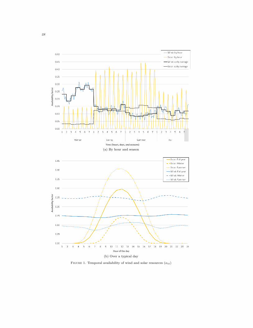
E. A first look at the data

Figure 1 plots the time-series data for αit showing in Panel (a) the hourly anddaily average availability by season over the course of a full year and in Panel (b)the availability by hour over a typical day of the full year, winter, and summerperiod. It is evident that there exists substantial heterogeneity in terms of thetemporal availability profiles of wind and solar resources. First, over a typical dayof a year and a given season, solar resources are much more volatile comparedto wind resources: while the availability profile for wind is relatively flat, solaris not available during evening and night hours and exhibits availabilities of upto 40% during the midday. Second, the seasonal availability patterns for thetwo resources differ. The availabilities of solar largely exceeds those for windduring the summer period (apart from night hours) which is reflected in the dailyaverages as well as the hourly profile over a typical day. Wind, however, hasa higher availability during the winter period for all hours during the day, thusexceeding the availability of solar during peak hours around midday. The hourlyprofiles for the spring and fall season represent intermediate cases (not shown)which are qualitatively similar to the hourly profile of an average day for the full

22Given the lack of clear-cut empirical evidence on the variation of the price-responsiveness of energydemand over hours of a day or seasons, we assume that ε is uniform across t.

23We use the year-2015 estimates from US Government Interagency Working Group on Social Costof Greenhouse Gases (2016) which are closest to our modelled base year. Our central-case value for δis close to the reported mean of $56 per ton of CO2 in the study); our high value for δ is based on ahigh-impact, low-probability scenario with “catastrophic” climate events.

28

(a) By hour and season

(b) Over a typical day

Figure 1. Temporal availability of wind and solar resources (αit)

29

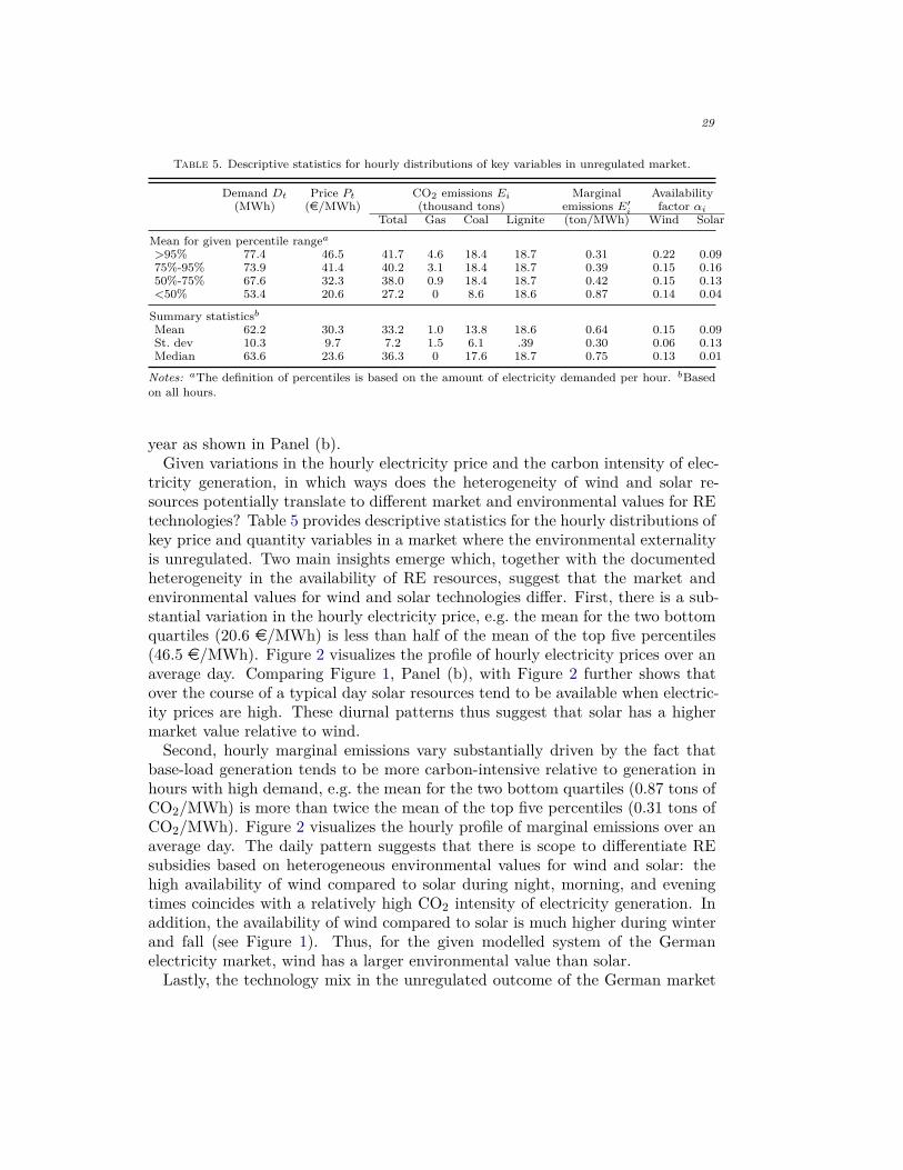
Table 5. Descriptive statistics for hourly distributions of key variables in unregulated market.

Demand Dt Price Pt CO2 emissions Ei Marginal Availability(MWh) (e/MWh) (thousand tons) emissions E′i factor αi

Total Gas Coal Lignite (ton/MWh) Wind Solar

Mean for given percentile rangea>95% 77.4 46.5 41.7 4.6 18.4 18.7 0.31 0.22 0.0975%-95% 73.9 41.4 40.2 3.1 18.4 18.7 0.39 0.15 0.1650%-75% 67.6 32.3 38.0 0.9 18.4 18.7 0.42 0.15 0.13<50% 53.4 20.6 27.2 0 8.6 18.6 0.87 0.14 0.04

Summary statisticsbMean 62.2 30.3 33.2 1.0 13.8 18.6 0.64 0.15 0.09St. dev 10.3 9.7 7.2 1.5 6.1 .39 0.30 0.06 0.13Median 63.6 23.6 36.3 0 17.6 18.7 0.75 0.13 0.01

Notes: aThe definition of percentiles is based on the amount of electricity demanded per hour. bBasedon all hours.

year as shown in Panel (b).Given variations in the hourly electricity price and the carbon intensity of elec-

tricity generation, in which ways does the heterogeneity of wind and solar re-sources potentially translate to different market and environmental values for REtechnologies? Table 5 provides descriptive statistics for the hourly distributions ofkey price and quantity variables in a market where the environmental externalityis unregulated. Two main insights emerge which, together with the documentedheterogeneity in the availability of RE resources, suggest that the market andenvironmental values for wind and solar technologies differ. First, there is a sub-stantial variation in the hourly electricity price, e.g. the mean for the two bottomquartiles (20.6 e/MWh) is less than half of the mean of the top five percentiles(46.5 e/MWh). Figure 2 visualizes the profile of hourly electricity prices over anaverage day. Comparing Figure 1, Panel (b), with Figure 2 further shows thatover the course of a typical day solar resources tend to be available when electric-ity prices are high. These diurnal patterns thus suggest that solar has a highermarket value relative to wind.

Second, hourly marginal emissions vary substantially driven by the fact thatbase-load generation tends to be more carbon-intensive relative to generation inhours with high demand, e.g. the mean for the two bottom quartiles (0.87 tons ofCO2/MWh) is more than twice the mean of the top five percentiles (0.31 tons ofCO2/MWh). Figure 2 visualizes the hourly profile of marginal emissions over anaverage day. The daily pattern suggests that there is scope to differentiate REsubsidies based on heterogeneous environmental values for wind and solar: thehigh availability of wind compared to solar during night, morning, and eveningtimes coincides with a relatively high CO2 intensity of electricity generation. Inaddition, the availability of wind compared to solar is much higher during winterand fall (see Figure 1). Thus, for the given modelled system of the Germanelectricity market, wind has a larger environmental value than solar.

Lastly, the technology mix in the unregulated outcome of the German market

30

Figure 2. Hourly wholesale electricity prices and hourly marginal emissions rate over a typical day

highly relies on coal-fired electricity: 89% of CO2 emissions derive from burninglignite and hard coal while only 11% stem from gas-fired generation (Table 5).Moreover, in the unregulated market there exist massive excess production capac-ities for natural gas (only 15.2% of the installed capacity for natural gas is used forelectricity generation). Together, these points suggest that there is considerablescope for CO2 abatement through switching from “dirty” to “clean” fossil fuels.

III. Main Simulation Results

This section compares the performance of optimal RE support schemes withregard to their ability to address the carbon externality.24 We first assess REsupport policies in terms of their welfare impact and investigate how particularfeatures of policy design affect the welfare implications. We then depart from theperspective of optimal RE policies by analyzing the policy ranking in terms ofcost-effectiveness, i.e. which RE policy can achieve a given emissions reductiontarget at the lowest possible cost.

24All simulations in this section are based on the central-case parametrization of the model as laidout in Section II.D More specifically, fuel prices, carbon coefficients, pre-installed production capacities,and empirically estimated marginal cost and emissions functions are specified according to Tables 3 and4, and we assume intermediate values for the own-price elasticity of energy demand (i.e., ε = −0.15) andthe social cost of carbon (i.e., δ = 50eper ton of CO2).

31

Figure 3. Comparison of efficient RE support policies

Notes: Assumes central case as specified in Section II.D. Legend: The “M” and “#” markers denote afeed-in tariff and market premium policy, respectively. Filled (hollow) triangles and circles refer to thecase when RE subsidies are uniform (differentiated) across wind and solar technologies. “Red” symbolsdenote the case when RE subsidies are combined in a revenue-neutral manner with a non-optimal energydemand tax. “Black” symbols denote the case when RE subsidies are combined with an optimal energydemand tax.

A. Can RE policies approximate the social optimum?

Figure 3 summarizes the welfare and CO2 emissions impacts (both measuredrelative to the unregulated market equilibrium) of the RE support policies whichhave been categorized in Table 1.25 We compare constrained-optimal RE policieswhich entail constraints on the structure and financing of RE subsidies. It isstraightforward to see that alternative regulatory designs can yield substantiallydifferent outcomes in an otherwise identical economy and given the same SCC.These differences stem from varying specific features of the RE support scheme:the structure of RE subsidies (uniform or technology-differentiated RE support),the financing of RE subsidies (demand tax vs. “polluter-pays-the-price”), and theway in which the expenses for RE subsidies and their financing are linked together(revenue-neutral support schemes or not).

First, carbon pricing achieves the highest welfare gain relative to the unregu-

25In contrast to the theoretical analysis, we focus in our numerical analysis on the case of a time-constant energy demand tax. First, a time-varying hourly demand tax is likely to be unrealistic from areal-world policy perspective. Second, the computational burden to solve for an optimal hourly demandtax would be enormous.

32

lated market outcome—consistent with the result that such a policy implementsthe social optimum (see Proposition 1).26 Second, RE support schemes which in-volve FIT or a market premium which are funded through a revenue-neutral taxon energy demand—marked by red triangles and circles—perform worst, yieldingless than 40% of the welfare gains obtained under carbon pricing. Third, differ-entiating RE subsidies, under either a FIT or a market premium, only negligiblyimproves overall economic efficiency—comparing solid with hollow triangles andcircles. Fourth, combining RE subsidies with an optimal demand tax to efficientlyincentivize the energy conservation channel, and thereby relaxing the constraintthat the energy demand tax is set to cover expenses for RE subsidies—comparingred with black triangles and circles—substantially enhances efficiency, yieldingabout twice the welfare gains relative to the revenue-neutral RE support schemes.However, such policies only achieve about 70% of the welfare gains associatedwith first-best carbon pricing. Fifth, changing the structure of refinancing of REsubsidies to one which charges conventional “dirty” energy producers in propor-tion to their emissions (i.e., “polluter-pays-the-price” financing), as would be thecase under a green offset policy, yields an outcome that is fairly close to the socialoptimum (achieving 80% of the welfare gains from carbon pricing).

B. Quantifying alternative designs for RE support

What are the economic mechanisms triggered by particular choices in the designof RE support policies and how do they explain the (in)ability to approximatesocially optimal outcomes? To compare policies, we define an index of abatementefficiency, Eb, which expresses the welfare change for an RE support policy brelative to the welfare change under the first-best carbon pricing policy:

(21) Eb = Wb −WWCarbon pricing −W

,

where W denotes welfare in the unregulated market equilibrium. The closer Eb

is to unity, the better the RE support policy b approximates the socially optimaloutcome.

TECHNOLOGY-NEUTRAL RE SUBSIDIES.—–RE support schemes based on a FIT ormarket premium with refinancing through energy demand taxes incentivize car-bon abatement through two channels. First, by subsidizing investments into REproduction capacity, they correct the relative prices between fossil-based and REtechnologies. Second, the refinancing tax increases the price of energy thus con-tributing to energy conservation.

Table 6 shows that the two channels are, however, not exploited in an efficientmanner. Tax-inclusive consumer prices increase only slightly (around 2%) leaving

26In our comparative-static analysis, reported welfare changes refer to annual values. For example,the 5.33% in the case of carbon pricing corresponds to a welfare increase equal to e0.236 billion per yearrelative to the unregulated market outcome.

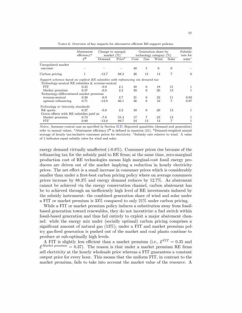
33

Table 6. Overview of key impacts for alternative efficient RE support policies.

Abatement Change to unregul. Generation share by Subsidyefficiencya market (%) technology category (%) rate forEb Demand Priceb Coal Gas Wind Solar solarc

Unregulated marketoutcome – – – 48 5 0 0 –

Carbon pricing 1 -12.7 88.3 26 13 14 7 0

Support schemes based on explicit RE subsidies with refinancing via demand taxTechnology-neutral RE subsidies & revenue-neutral

FIT 0.35 -0.8 2.1 30 0 18 15 1Market premium 0.37 -0.8 2.2 30 0 20 13 1

Technology-differentiated market premiumrevenue-neutral 0.38 -0.9 2.7 31 0 22 11 0.93optimal refinancing 0.71 -12.9 86.1 36 0 16 7 0.97

Technology or intensity standardsRE quota 0.37 -0.8 2.2 30 0 20 13 1Green offsets with RE subsidies paid as

Market premium 0.72 -7.8 55.4 17 7 23 13 1FIT 0.80 -13.0 89.7 24 13 13 7 1

Notes: Assumes central case as specified in Section II.D. Reported quantities (demand and generation)refer to annual values. aAbatement efficiency Eb is defined in equation (21). bDemand-weighted annualaverage of hourly tax-inclusive consumer prices for electricity. cSubsidy rate relative to wind. A valueof 1 indicates equal subsidy rates for wind and solar.

energy demand virtually unaffected (-0.8%). Consumer prices rise because of therefinancing tax for the subsidy paid to RE firms; at the same time, zero-marginalproduction cost of RE technologies means high marginal-cost fossil energy pro-ducers are driven out of the market implying a reduction in hourly electricityprices. The net effect is a small increase in consumer prices which is considerablysmaller than under a first-best carbon pricing policy where on average consumersprices increase by 88.3% and energy demand reduces by 12.7%. As abatementcannot be achieved via the energy conservation channel, carbon abatement hasbe to achieved through an inefficiently high level of RE investments induced bythe subsidy instrument: the combined generation share of wind and solar undera FIT or market premium is 33% compared to only 21% under carbon pricing.

While a FIT or market premium policy induces a substitution away from fossil-based generation toward renewables, they do not incentivize a fuel switch withinfossil-based generation and thus fail entirely to exploit a major abatement chan-nel: while the energy mix under (socially optimal) carbon pricing comprises asignificant amount of natural gas (13%), under a FIT and market premium pol-icy gas-fired generation is pushed out of the market and coal plants continue toproduce at sub-optimally high levels.

A FIT is slightly less efficient than a market premium (i.e., EFIT = 0.35 andEMarket premium = 0.37). The reason is that under a market premium RE firmssell electricity at the hourly wholesale price whereas a FIT guarantees a constantoutput price for every hour. This means that the uniform FIT, in contrast to themarket premium, fails to take into account the market value of the resource. A

34

FIT thus creates incentives for over-investment in solar capacity which are partic-ularly strong during periods of high demand (e.g., around noon) when electricityprices are high and solar availability is at its daily peak. Adding cheap solar en-ergy, in particular around midday, implies that hourly wholesale electricity pricesfall; RE firms, however, do not see these lower prices under a FIT scheme. Inaddition, a higher share of solar energy in total RE production under a FIT alsomeans that in winter, when the availability of solar is considerably lower, peak en-ergy demand is satisfied to a lesser extent with RE generation implying that morecarbon-intensive fossil generation is used and, hence, less carbon is abated. To-gether, these two effects explain the slightly lower efficiency of a FIT as comparedto a market premium.

TECHNOLOGY-DIFFERENTIATED RE SUBSIDIES.—–Proposition 2 states that optimalsubsidies for RE technologies should be differentiated according to the environ-mental value of the underlying resource. The relevant question for policy design,however, is: what order of magnitude for welfare gains can be achieved by opti-mally differentiating RE subsidies?

We find that improving policy design to reflect the environmental value ofthe underlying resource only produces minor efficiency gains (i.e., EMarket premium

increases from 0.37 for technology-neutral to 0.38 for technology-differentiatedRE subsidies; see Table 6).27 The reason is that wind has a higher environmentalvalue compared to solar over both daily and seasonal time scales (for the Germanelectricity market; see the analysis in Section II.E). The optimal differentiationof RE subsidies therefore entails a lower support rate for RE firms producingelectricity, i.e. the optimal subsidy rate for solar is 93% of the optimal subsidyrate for wind (see Table 6). Relative to the case of a technology-neutral REsupport, optimally differentiated subsidies thus lead to more investment in windand less investment in solar capacity.

COMBINING RE SUBSIDIES WITH AN OPTIMAL ENERGY DEMAND TAX.—–An optimalRE support scheme based on a FIT or market premium generates through the re-financing tax revenues which exceed the expenses for RE subsidies, i.e. an optimalFIT or market premium support policy cannot be revenue-neutral (see Corollary3). But how large is the efficiency gain when the revenue-neutrality constraint isrelaxed?

We find that combining RE subsidies, in the form of a FIT or market pre-mium, with an optimal energy demand tax yields sizeable improvements morethan doubling abatement efficiency (i.e., EMarket premium increases from 0.37 forrevenue-neutral to 0.71 for optimal refinancing; see Table 6). The optimal demandtax increases consumer prices to roughly the same levels as would be obtained un-der a carbon pricing policy, thus inducing similar abatement through the energyconservation channel. Importantly, we find that improving the refinancing of REsubsidies is more important than differentiating the subsidy rate by technology.

27From Corollary 1, we know that the optimal FIT and market premium lead to the same allocation.We here focus on discussing our results in terms of the market premium.

35

While the abatement efficiency increases when revenue-neutrality is relaxed, itstill is significantly below 1 because the demand tax does not affect the relativeproduction costs of coal vs. gas-fired electricity producers leaving the fuel-switchabatement channel unexploited.

INTENSITY STANDARDS FOR RE SUPPORT.—–Intensity standards are blending con-straints which translate into implicit output subsidies for RE technologies and im-plicit input taxes on energy production to finance RE subsidies. As such, they areby construction revenue-neutral, and cannot implement the social optimum (seeProposition 5). Notwithstanding their undesirable property of revenue-neutrality,we show below that intensity standards can in principle yield an abatement ef-ficiency fairly close to a first-best outcome depending on the structure of both(implicit) RE subsidies and the (implicit) input taxes to finance the RE support.

Under an RE quota an equal per-MWh tax on electricity is levied on all firmsto finance the RE subsidies. By construction, such a policy is revenue-neutral anddoes not discriminate the subsidy rate across RE technologies. An RE quota isthus equivalent to a technology-neutral market premium policy which is financedthrough a revenue-neutral tax on energy demand. Consequently, the abatementefficiency of an RE quota is poor (i.e., ERE quota = 0.37; see Table 6).

We find, however, that changing how RE subsidies are financed can greatlyenhance abatement efficiency. Under a green offset intensity standard, wheredemand for certificates is proportionally related to CO2 emissions, abatementefficiency increases (i.e., EGreen offsets is equal to 0.72 and 0.80 when the supportfor RE firms is structured as a subsidy added to the market price or a guaranteedoutput price, respectively). With respect to the performance of a green offsetssystem, three main insights emerge.

First, regardless of how the RE subsidies are structured, there is an advantagefor conventional energy producers with low emissions intensity due to the lowercosts for buying offset certificates for each MWh of electricity produced. Specifi-cally, this helps to exploit carbon abatement through the fuel-switch channel byincentivizing electricity generation from natural gas.

Second, when the subsidies for RE firms are structured as a market premium,the abatement efficiency of a green offset system is only slightly higher than underan optimal policy with technology-differentiated market premium and demand taxrefinancing. The reason is that when the marginal damage of emissions is reflectedthrough the implicit input taxes, the wholesale electricity price already reflectsthe external cost. There is thus no need to further subsidize RE investments,i.e. the subsidy rate for RE firms should be zero. This, however, is not whathappens under green offsets policy: revenue neutrality implies that positive taxrevenues translate into a positive subsidy rate which is added on top of the whole-sale electricity price, thus yielding inefficiently high unit revenues per MWh ofelectricity produced from wind and solar resources. In addition, the inefficientlyhigh subsidy rate dampens the price signal for energy conservation. We find thatwhen RE subsidies are paid as a market premium, the advantage of implicitly

36

taxing CO2 emissions under a green offsets system, which induces a partial fuelswitch to natural gas, is almost entirely outweighed by too high investments intoRE technologies and a too low energy demand reduction.

Third, as under a FIT investors do not receive the wholesale price. the abate-ment efficiency increases because the induced over-investment in wind and solaris much smaller as compared to a market premium. At the same time, the needfor refinancing is higher when RE support is paid in the form of a guaranteedoutput price relative to a market premium. A higher need for refinancing, how-ever, implies a stronger carbon price signal established through the implicit inputtaxes. This explains why the green offsets system with FIT can come closer tothe socially optimal outcome obtained under carbon pricing.

C. Cost-effective RE support policies

Rather than choosing optimal RE support policies under an endogenous envi-ronmental target (and given information about the SSC), policymakers may alsobe concerned with the question which policy designs can achieve a given emissionsreduction target at lowest economic cost. To scrutinize the cost-effectiveness per-spective on optimal policy choice, this section considers a simplified version ofthe general problem of optimal regulation laid out in (4), or its numerical equiv-alent (11), by assuming that RE support policy has to achieve an exogenouslydetermined and fixed level of emissions reductions, E.28

Figure 4 shows the percentage welfare change relative to the unregulated marketoutcome (i.e., 100× [Wb/W− 1]) for different RE support schemes b for differentlevels of emissions. Unsurprisingly, carbon pricing is the most cost-effective policyirrespective of policy stringency as it efficiently exploits all abatement channels.The “cost-effectiveness ranking” of RE support policies, however, varies largelydepending on policy stringency. Generally speaking, the reason is that alternativepolicy designs exploit various abatement channels (see Table 2) differently whilethe relative importance of each abatement channel for total abatement variesdepending on targeted emissions reductions.

Analyzing the policy ranking under cost-effectiveness considerations yields thefollowing additional insights with respect to the performance of different RE sup-port schemes. First, the technology differentiation of RE subsidies according tothe heterogeneous environmental value of the underlying resource is empiricallynot important for policy design at any level of emissions reductions. This under-scores the similar finding we obtained in the context of optimal RE policies withendogenous environmental quality.

Second, for high abatement levels (i.e., emissions reductions relative to theunregulated market outcome are in excess of 50%), it becomes crucial to link the

28Specifically, we add the following constraint to the upper-level part of the optimal policy problem in(11):

∑i,t

∫ Xit

0 Ei(x)dx ≤ E. This amounts to evaluating policy choices solely on the basis of economicsurplus—while the differences in environmental benefits from averted pollution are muted across thepolicy options given a constant environmental quality.

37

Figure 4. Cost-effectiveness of RE support under varying policy stringency

financing of RE support to carbon-intensive generation, for example, as achievedthrough an intensity standard with green offset certificates. The reason is that thehigher policy stringency, the more important becomes CO2 abatement throughswitching from coal to natural gas. As RE support schemes based on either a FITor market premium fail to incentivize such a fuel switch, they perform poorly. Thisholds regardless of whether such policies are combined with an optimal demandtax for refinancing or not. With increasing policy stringency, green offsets withRE subsidies paid through a FIT outperform a green offset scheme with a marketpremium as a guaranteed output price under a FIT avoids over-investment in REcapacity (this is similar to the context of optimal RE support with endogenousenvironmental quality; see Section III.A).

Third, for intermediate abatement levels (between 20% and 50%), abatementis mainly achieved through RE capacity investments and reductions in energy de-mand; the switch with fossil-based technologies is not important. For this rangeof emissions reductions, RE subsidies with an optimal energy demand tax arethus the second-best policy (after carbon pricing). In particular, they outper-form all policy designs which require revenue-neutrality between RE subsidiesand refinancing. The reason is that the revenue-neutrality requirement limits thescope for exploiting abatement through the energy conservation channel. Withincreasing policy stringency, the green offset policies begin to outperform the REsupport schemes with revenue-neutral demand tax refinancing as the efficiencygains from incentivizing a fuel-switch increase.

Fourth, for low abatement levels (less than 20%), cost-effective abatement under

38

a carbon pricing policy mainly occurs through energy conservation. The perfor-mance of revenue-neutral RE policies relative to , either directly as in the case ofa FIT or market premium or indirectly under a green offset intensity standard,is therefore rather poor for low policy stringency as they entail inefficiently highincentives for RE investments averting abatement through energy conservationwith to increase the consumer price.29

IV. Robustness Checks and Model Extensions

Here we consider the sensitivity of results to parameters and model extensionsaffecting the relative importance of the different channels for abatement includingthe price responsiveness of energy demand, fuel prices and the composition of in-stalled fossil-based production capacities, the social cost of carbon, environmentaldamages due to non-CO2 greenhouse gases, and a higher temporal resolution.

A. Price responsiveness of energy demand

Columns (1)–(3) in Table 7 compare the abatement efficiency Eb of the differentRE support schemes for different assumptions about the price elasticity of energydemand (|ε|). The stronger demand responds to price, the easier it is to induceabatement through the energy conservation channel for a given consumer priceincrease. Hence, the gap in abatement efficiency between carbon pricing andpolicies which subsidize RE technologies without refinancing rules that counteracttoo low energy prices, i.e. RE subsidies with revenue-neutral demand tax financingand RE quota, is larger (smaller) for the case of a high (low) |ε|. In contrast, theabatement efficiency of RE support schemes which combine RE subsidies withan optimal demand tax depends positively on |ε| as such a policy can directlyincentivize abatement through reductions in energy demand.

For a market where energy demand is relatively price-elastic, Table 7 showsthat green offsets policies can closely approximate the socially optimal outcome(i.e., EGreen offsets equals 0.82 and 0.92 for the case of FIT and market premium, re-spectively). Intuitively, if the energy conservation channel is relatively important,the distortion induced by such policies—due to the fact the environmental dam-age is already reflected in electricity prices and that RE firms receive in additiona positive subsidy rate leading to abatement through an over-investment in REcapacity—becomes less important. On the other hand, the abatement efficiencyof such policies can be poor, when |ε| is low.

B. Low natural gas prices and “monolithic” fossil-based energy supply

An important question is how our assessment of alternative policy designs forRE support changes when it becomes less important or even not necessary at all to

29The case of the market premium with optimal demand tax refinancing is not shown for low abatementlevels as this policy would essentially involve taxing energy demand with a zero subsidy rate for REtechnologies.

39

Table 7. Sensitivity of abatement efficiency Eb of different RE support policiesa.

Central Demand elasticity Low natural Monolithic High SSCcaseb ε = −0.05 ε = −0.5 gas pricec FE supply δ = 100

(1) (2) (3) (4) (5) (6)

Support schemes based on explicit RE subsidies with refinancing via demand taxTechnology-neutral RE subsidies & revenue-neutral

FIT 0.35 0.44 0.26 0.23 0.42 0.67Market premium 0.37 0.45 0.29 0.23 0.42 0.72

Technology-differentiated market premiumrevenue-neutral 0.38 0.46 0.30 0.23 0.42 0.75optimal refinancing 0.71 0.63 0.76 0.68 0.94 0.81

Technology or intensity standardsRE quota 0.38 0.46 0.30 0.23 0.94 0.75Green offsets with RE subsidies paid as

Market premium 0.72 0.66 0.82 0.50 0.06 0.97FIT 0.80 0.69 0.92 0.55 0 0.85

Notes: aEb is defined by equation (21). bThe central-case values are: ε = −0.15 and δ = 50e per tonof CO2. cAssumes that the fuel price for natural gas is reduced from the central-case value of 21.16e/MWh to 5 e/MWh.

switch from coal to natural gas in order to reach a social optimum. To explore thisquestion, we analyze the two additional cases assuming (1) a substantially lowernatural gas price (reducing central-case value of 21.16 e/MWh to 5 e/MWh) and(2) that all coal-fired (lignite and hard coal) capacity is rededicated as naturalgas capacity.

Both perspectives are useful to reflect the conditions of current and likely fu-ture energy systems. First, the costs of supplying natural gas may decline furtherdue to increased exploitation of shale gas resources and enhanced infrastructureand market integration due to liquified natural gas. Second, systems with “mono-lithic ” fossil-based energy (FE) supply not only depict the current situation ofa number of countries with abundant oil resources (for example, Middle Easterncountries such as Iran, Saudia Arabia, Egypt) but may also describe future elec-tricity systems for countries where coal use has already been banned or wherenuclear power in an otherwise zero-carbon generation mix will be replaced withnatural gas (for example, Sweden and Switzerland).

In the case with a “Low natural gas price” (comparing columns (1) and (4) inTable 7), the technology mix in the unregulated market outcome, compared tothe central case (see Table 6), is tilted towards natural gas (generation share of29.7%) but coal is still part of the mix (generation share of 32.2%). While thisreduces the scope for CO2 abatement through a fuel switch between coal andgas, the important implication of low natural gas prices is another one: for thesocially optimal policy with carbon pricing, the tax-inclusive fuel price of coal ishigher than the one for natural gas. This implies that coal-fired plants becomeprice-setting with the result that the increase in the consumer price of electricityis substantially larger than in a situation with high natural gas prices. Conse-quently, the abatement efficiency of RE support policies which do not exploit

40

the energy conservation channel relative to carbon pricing significantly worsens.The important implication for policy design is that as long as coal-based genera-tion remains in the system, the efficiency loss associated with using RE supportschemes, without modifying the financing structure to reflect the carbon intensityof fossil-based generation, may be substantial.30

In contrast, when no fuel switch is needed, as is the case for systems with “Mono-lithic FE supply”, RE support schemes have the ability to closely approximatethe socially optimal outcome obtained with carbon pricing. The extent to whichthis is possible, however, depends on whether the RE support scheme can trig-ger abatement through the energy conservation channel. If this is possible onlyto a limited extent, as under a revenue-neutral FIT or market premium system,the abatement efficiency remains poor (i.e., EFIT = EMarket premium = 0.42). Apolicy combining optimal RE subsidies with optimal refinancing yields an abate-ment efficiency which closely approximates those obtained under first-best carbonpricing (i.e., EMarket premium with optimal demand tax = ERE quota = 0.94). With an op-timal time-varying hourly demand tax such policies would achieve the first-bestsolution (see Proposition 4); the remaining efficiency loss thus derives from con-straining the optimal demand tax to be uniform over time.

C. Social cost of carbon

The higher the SCC, the higher is in general the abatement efficiency of REsupport schemes, i.e. Eb increases for all policies (comparing column (6) to column(1) in Table 7). The simple reason is that with higher SCC abatement mainlyoccurs through subsidizing RE investments and conserving energy demand whilethe importance of a fuel switch among fossil-based generation is diminished.

But even with high SCC, the question of policy design remains important. Sup-port schemes that either establish incentives for energy conservation or are basedon “polluter-pays-the-price” financing of RE subsidies can closely approximatesocially optimal outcomes (i.e., the abatement efficiency exceeds 80%) whereasrevenue-neutral FIT or market premium policies entail efficiency losses of around30% (i.e., EFIT = 0.67 and EFIT = 0.72).

D. Non-CO2 greenhouse gases

Motivated by the fact that CO2 is the principal anthropogenic greenhouse gas(GHG) being emitted by the power sector, we have so far abstracted from othernon-CO2 GHGs relevant in the context of electricity generation such as methane(CH4) and nitrous oxide (N2O). The potential concern is that not accounting forother GHGs may underestimate the potential benefits from RE support schemesrelative to carbon pricing policies. While a carbon pricing policy provides incen-

30One exception is the RE policy which combines RE subsidies with an optimal demand tax. Here,the possibility to directly incentivize energy conservation somewhat dampens the efficiency loss (i.e.,EMarket premium with optimal demand tax = 0.68).

41

tives for removing coal, it potentially leaves a significant amount of natural gas,and hence methane emissions, in the system. In contrast, a stringent RE supportpolicy provides incentives for removing fossil fuels altogether.

Although these GHGs are more potent than CO2, we find that including themexplicitly in our analysis does not affect our main insights—and, in fact, only hassmall quantitative effects (for example, on abatement efficiency Eb as our mainmetric for comparing policies). The robustness of our results with respect to theinclusion of non-CO2 GHGs can be understood as follows. First, the amounts ofnon-CO2 GHGs are several orders of magnitude smaller than for CO2. Second,the ordering of energy technologies in terms of emissions intensity is not altered.More specifically, for the case of CH4, the emissions coefficient for natural gasand different types of coal is roughly identical; for N2O, natural gas has a loweremissions coefficient than coal.31

Consequently, including non-CO2 GHGs in our model slightly increases, onaverage, the damage caused by a MWh of electricity produced. The upshotis that under all policies considered a higher level of abatement is optimal (ascompared to ignoring non-CO2 GHGs). As the ordering of energy technologies,including the costs due to environmental damage caused, does not change, thequalitative ranking among different regulatory designs for addressing the GHGexternality are unaffected.

E. Temporal resolution

While we model electricity supply and demand decisions at the hourly level,we use for each season the hours of an average week to reduced computationalcomplexity (rather than using all 8760 hours of a year). The potential concern isthat this may smooth out some of temporal variation with respect to the avail-ability of RE resources and energy demand. While solving the model for 8760hours is computationally not feasible, we have carried out sensitivity analysisbased on a model with 12 (instead of four) representative weeks. We find thatthis increases the temporal variation of marginal hourly emission rates thus poten-tially pronouncing the scope for technology-differentiated RE subsidies. We dofind, however, that the optimal differentiation of the subsidy rate between windand solar is only slightly affected, suggesting that four representative weeks aresufficient to capture the variability of resource availability and demand relevantfor our analysis.

V. Conclusions

Public policies aimed at promoting clean energy from intermittent RE resourcessuch as wind and solar are the most widely adopted form of actual low-carbon

31Using standard emissions coefficients and CO2-equivalence factors of global warming potentials forCH4 and N2 from the IPCC (see tables 2.2 and 2.14 in Eggleston et al., 2006), the emissions factors forcoal and natural gas increase by only 0.5% and 0.09%, respectively.

42

policy—yet the question of how to best design support schemes for wind and solarhas received surprisingly little attention. This paper aims to fill this gap by exam-ining optimal support schemes for intermittent RE resources in the presence ofa carbon externality. We have characterized optimal policies and the conditionsunder which RE support schemes can achieve socially optimal outcomes. To as-sess different policies in an empirically plausible setting and to derive additionalquantitative insights, we have developed a numerical equilibrium framework of op-timal policy design which incorporates a number of features relevant for analyzingreal-world electricity markets.

We have emphasized three issues for policy design: the heterogeneity of in-termittent natural resources, budget-neutral financing rules, and incentives forcarbon mitigation. We show that optimal subsidies for wind and solar should bedifferentiated to reflect the heterogeneous environmental value of the underlyingresource. We find, however, that the differentiation of RE subsidies is only ofminor importance for policy design. Rather, the way RE subsidies are financedis critical: RE policies relying on “smart” financing by either using “polluter-pays-the-price” financing in the context of budget-neutral schemes (such as, forexample, RE quotas and technology or intensity standards for clean energy) orby giving up budget neutrality can approximate socially optimal outcomes. Wehave further assessed the performance of RE policies under different market condi-tions (including the price responsiveness of energy demand and the composition offossil-based supply) and assumptions about the social valuation of environmentaldamages (including the social cost of carbon and inclusion of non-CO2 greenhousegases). Overall, our analysis suggests that—when carbon pricing is unavailabledue to political (and other) constraints—optimally designed RE support policiesdo not necessarily have to be regarded as a costly second-best option.

Some limitations of our analysis should be kept in mind. First, our analysis hasfocused on how to design RE support policies in the presence of a carbon exter-nality. In doing so, we have deliberately abstracted from the positive externalitiesrelated to learning, technological innovation through R&D investments, and net-work effects (Jaffe, Newell and Stavins, 2005; Acemoglu et al., 2012; Bollingerand Gillingham, 2014) which may provide an important rationale for choosingRE support schemes over carbon pricing policies. Incorporating such positive ef-fects would obviously play in favor of RE support policies. Second, these benefitswould, however, have to be weighed against the additional system integration andback-up cost of intermittent RE generation (Borenstein, 2012; Marcantonini andEllerman, 2014; Gowrisankaran, Reynolds and Samano, 2016). While it is beyondthe scope of this paper to provide a comprehensive cost-benefit analysis, our es-timates could be viewed as a first indication of how large the net benefits fromother external effects would have to be to provide a rationale for decarbonizationthrough RE support policies.

Notwithstanding these caveats, our analysis demonstrates that optimally de-signed policies to support RE from intermittent wind and solar resources, in par-

43

ticular with regard to the financing of RE subsidies, can substantially enhance theefficiency of decarbonization policies in the electricity sector. At the same time,this diminishes the importance of arguments relying on positive (and difficult toquantify) learning and technology externalities for rationalizing the public policysupport for renewable energy.

REFERENCES

50Hertz. 2018. “Wind Production in the German Region Controlled by 50Hertz.” accessed 2018.http://www.50hertz.com/en/Grid-Data/Wind-power/Archive-Wind-power.

Abrell, Jan, Mirjam Kosch, and Sebastian Rausch. 2017. “How “Green” are the Wind and theSun? European Renewable Energy Policies and Carbon Abatement.” Working Paper 2017.

Acemoglu, Daron, Philippe Aghion, Leonardo Bursztyn, and David Hemous. 2012. “TheEnvironment and Directed Technical Change.” American Economic Review, 102(1): 131–166.

Agentur fur Erneuerbare Energien. 2017. “Foderal Erneurbar: Bundeslander mit neuer Energie.”https://www.foederal-erneuerbar.de/uebersicht/bundeslaender/.

Ambec, Stefan, and Claude Crampes. 2012. “Electricity provision with intermittent source ofEnergy.” Resource and Energy Economics, 34: 319–336.

Ambec, Stefan, and Claude Crampes. 2017. “Decarbonizing electricity genera-tion with intermittent sources of energy.” Unpublished working paper. Available at:https://pdfs.semanticscholar.org/6f7b/3f405842c24394c02f99d2f0d8156c5d2f3e.pdf.

Amprion. 2018. “Wind Production in the German Region Controlled by Amprion.” accessed 2018.https://www.amprion.net/Netzkennzahlen/Windenergieeinspeisung/index-3.html.

Baumol, W J. 1972. “On Taxation and the Control of Externalities.” American Economic Review,62(3): 307–322.

Bollinger, B. K., and K. Gillingham. 2014. “Learning-by-doing in solar photovoltaic installations.”Technical report.

Borenstein, Severin. 2012. “The private and public economics of renewable electricity generation.” TheJournal of Economic Perspectives, 26(1): 67–92.

Callaway, Duncan, Meredith Fowlie, and Gavin McCormick. 2017. “Location, Location, Loca-tion: The Variable Value of Renewable Energy and Demand-side Efficiency Resources.” Journal ofthe Association of Environmental and Resource Economists, 5(1): 39–75.

Carbone, Jared C., and V. Kerry Smith. 2008. “Evaluating Policy Interventions with GeneralEquilibrium Externalities.” Journal of Public Economics, 92(5): 1254–1274.

Crew, Michael A., and Paul R. Kleindorfer. 1976. “Peak Load Pricing with a Diverse Technology.”The Bell Journal of Economics, 7(1): 207–231.

Crew, Michael A, Fernando S. Chitru, and Paul R. Kleindorfer. 1995. “The Theory of Peak-Load Pricing: A Survey.” Journal of Regulatory Economics, 8: 215–248.

Cullen, Joseph. 2013. “Measuring the Environmental Benefit of Wind-Generated Electricity.” AmericanEconomic Journal: Economic Policy, 5(4): 107–133.

Dirkse, Steven P., and Michael C. Ferris. 1995. “The PATH Solver: A Non-Monotone StabilizationScheme for Mixed Complementarity Problems.” Optimization Methods and Software, 5: 123–156.

Edenhofer, Ottmar, Jan Christoph Steckel, Michael Jakob, and Christoph Bertram.2018. “Reports of coal’s terminal decline may be exaggerated.” Environmental Research Letters,13(2): 024019.

Eggleston, H.S., L. Buendia, K. Miwa, T. Ngara, and K. Tanabe. 2006. “2006 IPCC Guidelinesfor National Greenhouse Gas Inventories.” IPCC.

EnergyCharts. 2015. “German Generation Data; https://www.energy-charts.de/power de.htm.”ENTSO-E. 2016. “Hourly electricity consumption.” https://www.entsoe.eu/db-

query/consumption/mhlv-a-specific-country-for-a-specific-month.EPEX. 2015. “Hourly Dayahead Prices; https://www.epexspot.com/en/.”European Commission. 2010. “Renewable Energy Directive (2009/28/EC).”Fell, Harrison, and Joshua Linn. 2013. “Renewable electricity policies, heterogeneity, and cost effec-

tiveness.” Journal of Environmental Economics and Management, 66: 688–707.

44

Fischer, Carolyn, and Richard G Newell. 2008. “Environmental and technology policies for climatemitigation.” Journal of environmental economics and management, 55(2): 142–162.

Fullerton, Don, and Garth Heutel. 2005. “The General Equilibrium Incidence of EnvironmentalTaxes.” National Bureau of Economic Research Working Paper 11311.

Goulder, Lawrence H., and Ian W. H. Parry. 2008. “Instrument Choice in Environmental Policy.”Review of Environmental Economics and Policy, 2(2): 152–174.

Goulder, Lawrence H., Marc A. C. Hafstead, and III Williams, Roberton C. 2016. “GeneralEquilibrium Impacts of a Federal Clean Energy Standard.” American Economic Journal: EconomicPolicy, 8(2): 186–218.

Gowrisankaran, Gautam, Stanley S. Reynolds, and Mario Samano. 2016. “Intermittency andthe Value of Renewable Energy.” Journal of Political Economy, 124(4): 1187 – 1234.

Helm, Carsten, and Mathias Mier. 2016. “Efficient diffusion of renewable energies: A roller-coasterride.” Oldenburg Discussion Papers in Economics, VŰ389Ű16: 1–30.

Holland, Stephen P., Jonathan E. Hughes, and Christopher R. Knittel. 2009. “GreenhouseGas Reductions under Low Carbon Fuel Standards?” American Economic Journal: Economic Policy,1(1): 106–146.

Jaffe, Adam B., Richard G. Newell, and Robert N. Stavins. 2005. “A tale of two market failures:Technology and environmental policy.” Ecological Economics, 54: 164–174.

Kaffine, Daniel T, Brannin J McBee, and Jozef Lieskovsky. 2013. “Emissions savings from windpower generation in Texas.” The Energy Journal, 34(1): 155–175.

Kalkuhl, Matthias, Ottmar Edenhofer, and Kai Lessmann. 2015. “Renewable energy subsidies:Second-best policy or fatal aberration for mitigation?” Resource and Energy Economics, 35: 217–234.

Kost, Christoph, Johannes N. Mayer, Jessica Thomsen, Niklas Hartmann, CharlotteSenkpiel, Simon Philipps, Sebastian Nold, Simon Lude, Noha Saad, and Thomas Schlegl.2013. “Levelized Cost of Electricity: Renewable Energy Technologies.” Frauenhofer Institute for SolarEnergy Systems ISI Study.

Luo, Zhi-Quan, Jong-Shi Pang, and Daniel Ralph. 1996. Mathematical programs with equilibriumconstraints. Cambridge University Press.

Marcantonini, Claudio, and A Denny Ellerman. 2014. “The implicit carbon price of renewableenergy incentives in Germany.” Robert Schuman Centre for Advanced Studies Research Paper No.RSCAS, 28.

Mathiesen, Lars. 1985. “Computation of economic equilibria by a sequence of linear complementarityproblems.” Economic Equilibrium: Model Formulation and Solution, , ed. Alan S. Manne, 144–162.Berlin, Heidelberg:Springer Berlin Heidelberg.

Meckling, Jonas, Thomas Sterner, and Gernot Wagner. 2017. “Policy sequencing toward decar-bonization.” Nature Energy, 2: 918–922.

Metcalf, Gilbert E. 2009. “Market-Based Policy Options to Control U.S. Greenhouse Gas Emissions.”Journal of Economic Perspectives, 23(2): 5–27.

Novan, Kevin. 2015. “Valuing the wind: renewable energy policies and air pollution avoided.” AmericanEconomic Journal: Economic Policy, 3(7): 291–326.

Open Power System Data. 2017. “Conventional power plants Germany.” https://data.open-power-system-data.org/conventional power plants/.

Rausch, Sebastian, and Matthew Mowers. 2014. “Distributional and Efficiency Impacts of Cleanand Renewable Energy Standards for Electricity.” Resource and Energy Economics, 36(3): 556–585.

REN, (Renewable Energy Network for the 21st Century). 2017. “Renewables 2017 Global StatusReport.” Available at: http://www.ren21.net/status-of-renewables/global-status-report/.

Rutherford, Thomas F. 1995. “Extension of {GAMS} for complementarity problems arising in appliedeconomic analysis.” Journal of Economic Dynamics and Control, 19(8): 1299 – 1324.

Tennet. 2018. “Wind Production in the German Region Controlled by Tennet.” accessed2018. http://www.tennettso.de/site/Transparenz/veroeffentlichungen/netzkennzahlen/tatsaechliche-und-prognostizierte-windenergieeinspeisung.

Tietenberg, T. H. 2013. “Reflections–carbon pricing in practice.” Review of Environmental Economicsand Policy, 7: 313–329.

TransnetBW. 2018. “Wind Production in the German Region Controlled by TransnetBW.” accessed2018. https://www.transnetbw.de/de/transparenz/marktdaten/kennzahlen.

U.S. Department of Energy. 2016. “Database of State Incentives for Renewables & Efficiency.”

45

http://www.dsireusa.org/.US Government Interagency Working Group on Social Cost of Greenhouse Gases. 2016.

“Technical Support Document: Technical Update of the Social Cost of Carbon for Regulatory ImpactAnalysis Under Executive Order 12866.” .

Wibulpolprasert, Wichsinee. 2016. “Optimal environmental policies and renewable energy invest-ment: evidence from the texas electricity market.” Climate Change Economics, 7(4).

46

Appendix A: Proofs

A1. Proof of Proposition 1

Let te = κi, ∀i, denote the uniform emissions tax. Maximizing the social surplus (2) with respect toκ yields the following first-order condition:

(A1)∑t

[S′t∂dt

∂te−G′t

∂kt

∂te

]=∑i,t

(C′it + δE′it

) ∂qit∂te

.

From the equilibrium conditions for conventional energy production (4b) and RE generation (4c), weobtain, respectively: C′ct ≥ C′dt = pt − teE′dt and S′t = G′t = pt. Differentiating the market-clearingcondition (4d) with respect to te yields:

∑i∂qit∂te

= ∂dt∂te

. Substituting terms into (A1) gives:∑t

pt∑i

∂qit

∂te=∑t

(pt − teE′t + δE′t

)∑i

∂qit

∂te,

which can be simplified to yield:te = δ .

From comparing the conditions for the social optimum (3a) with the equilibrium conditions (4b) underthe case of carbon pricing only (i.e., st = τt = 0), it follows that a uniform carbon tax κi = te = δ, ∀i,implements the social optimum. �

A2. Proof of Proposition 2

We present the proof for the case of an RE support scheme consisting of a FIT and tax on energydemand. The proof for the case of a market premium proceeds analogously.

As we know from Proposition 3 that the clean technology does not enter the market, we can focuson the dirty conventional generation technology, i.e. we can simplify notation by dropping the index forconventional technologies. Differentiating the equilibrium conditions (4a)–(4d) for the case of a FIT withrespect to the RE subsidy (st) yields:

∂kt

∂st=

1G′′t

∂dt

∂st=

C′′tC′′t − S′′t

∂kt

∂st

∂qt

∂st=

S′′tC′′t − S′′t

∂kt

∂st

∂pt

∂st=

C′′t S′′t

C′′t − S′′t

∂kt

∂st,

and with respect to a change in the energy demand tax (τt) yields:

∂kt

∂τt= 0

∂dt

∂τt=∂qt

∂τt=

1S′′t − C′′t

< 0

∂pt

∂τt=

C′′tS′′t − C′′t

< 0 .

From the regulator’s problem in (4), we can derive the following first-order conditions for optimal feed-in

47

tariffs (st) and energy demand taxes (τt), respectively, as:

S′t∂dt

∂st−(C′t + δE′t

) ∂qt∂st−G′t

∂kt

∂st= 0

S′t∂dt

∂τt−(C′t + δE′t

) ∂qt∂τt−G′t

∂kt

∂τt= 0 .

Since the RE firm only receives the feed-in tariff, the RE capacity kt does not respond to a change in thedemand tax, i.e. ∂kt

∂τt= 0. Substituting the marginal private surplus, conventional cost, and marginal

investment cost from the equilibrium conditions and using the partial derivatives of conditions (4d) forclearing of the energy spot markets with respect to the RE subsidy and demand tax yields:

(pt − st)∂kt

∂st+ tt

∂dt

∂st− δE′t

∂qt

∂st= 0(

tt − δE′t) ∂dt∂tt

= 0 .

From the second equation above, the socially optimal level of the energy demand tax can be derived as:

τ∗t = δE′t .

Inserting τ∗t into the first equation above and using the derived terms for the equilibrium responses ofkt, dt, and qt with respect to RE subsidies st yields:

s∗t = pt + δE′t .

�

A3. Proof of Corollary 2

Proof of parts (i) and (iii): A constant surplus function St implies that energy demand is constantover time. Hence, conventional energy production is constant over time, too. Given that cost functionCit(qit) and the emissions function Eit(qit) are time-invariant, this implies that the wholesale energyprice and the emissions level do not change over time. From the formula for the optimal FIT in equation(8a) it then follows that the FIT rate has to be differentiated by t, i.e. across RE technology or REresource. Similarly, if marginal costs (the emissions rate) are constant, the wholesale energy price (theemissions rate) takes on the same value for all t, implying that the optimal FIT is constant over time,i.e. s∗FIT1 = s∗FIT2 . The proof for the case of an optimal market premium proceeds analogously.

Proof of part (ii): With the same reasoning, if the surplus is constant in time or the marginal emissionsrate is constant, the marginal social costs are constant in time and, thus the demand tax is constant intime, i.e. τ∗1 = τ∗2 . �

A4. Proof of Corollary 3

The revenues from an energy demand tax (weakly) exceed the expenses for an RE subsidy which isstructured as a market premium if: ∑

t

τtdt ≥∑t

stkt

and for an RE subsidy which is structured as a FIT if:∑t

τtdt ≥∑t

(st − pt) kt .

48

Using the respective optimal RE subsidy rate and demand tax from Proposition 2 yields:∑t

δE′dtdt ≥∑t

δE′dtkt

which always holds since marginal emissions rates are positive and energy demand (weakly) exceedsthe production of renewable sources. If the market penetration of RE is incomplete, i.e. kt < dt, thetax revenues under an optimal RE support scheme is strictly larger than the expenses for optimal REsubsidies. �

A5. Proof of Proposition 3

We prove Proposition 3 for the case of a FIT.32 Differentiating the equilibrium conditions (4a)–(4d)under the case of a FIT (i.e., κi = τt = 0) with respect to feed-in rates st and solving for the policy-induced changes in equilibrium quantities and prices yields:

∂kt

∂st=

1G′′t

> 0

∂dt

∂st=∂dt

∂kt

∂kt

∂st=

∑iC′′it∑

iC′′it − S

′′t

∂kt

∂st=

∑iC′′it∑

iC′′it − S

′′t

1G′′t

> 0

∂qit

∂st=∂qit

∂kt

∂kt

∂st=

∑jC′′jt∑

jC′′jt − S

′′t

S′′tC′′it

∂kt

∂st=

∑jC′′jt∑

jC′′jt − S

′′t

S′′tC′′it

1G′′t

< 0

∂pt

∂st=∂pt

∂kt

∂kt

∂st=

∑iC′′it∑

iC′′it − S

′′t

S′′t∂kt

∂st=

∑iC′′it∑

iC′′it − S

′′t

S′′t1G′′t

< 0 .

The FIT thus implies an increase in demand and a reduction in the price of electricity. Moreover, itunambiguously increases generation from RE technologies and reduces output from the clean and dirtyconventional technology. Recalling that the clean conventional technology is initially not in the marketimplies that it does not enter the market due to a FIT. The weaker statement of this result—if one wereto relax the assumption that the clean technology is initially not in the market—is to say that the outputof the clean technology decreases due to the introduction of a FIT. As long as the cost functions of theconventional technologies are convex and do not intersect, however, it holds that the FIT does not leadto a fuel switch between clean and dirty conventional technologies.

Similarly, equilibrium changes in response to a change in demand taxes are given by:

∂kt

∂tt= 0

∂qit

∂tt=

∏iC′′it

S′′t∑

iC′′it −

∏iC′′it

1C′′it

< 0

∂dt

∂tt=∑i

∂qit

∂tt< 0

∂pt

∂tt=

∏iC′′it

S′′t∑

iC′′it −

∏iC′′it

< 0 .

Applying the same argumentation as above, it is straightforward to see that a demand tax does notcreate a fuel switch between the two conventional technologies. �

32The proof for the case of a market premium proceeds analogously and is omitted for reasons ofbrevity.

49

A6. Proof of Proposition 4

Suppose the social optimum does not require a fuel switch, that is, the cleaner conventional energytechnology c does not enter the market following a direct or indirect RE support policy, i.e. qct = 0.From Proposition 3, it follows that the clean conventional technology never enters the market under anRE subsidy. Substituting the optimal RE subsidy, either for the case of a FIT or a market premium,as well as the optimal energy demand tax from Proposition 2 into the equilibrium conditions (4a)–(4d)yields:

S′t = pt + δE′t ∀tC′t = pt ∀tG′t = pt + δE′t ∀t

⇒ S′t = C′t + δE′t = G′t ∀t

which is equivalent to the conditions characterized by (3a) and (3b). In contrast, suppose the socialoptimum implements an allocation in which production of the clean conventional energy technology c ispositive, i.e. qct > 0. From Proposition 3 technology c never enters the market under an RE subsidy; anRE subsidy therefore does not implement the social optimum.

50

Appendix C: Additional Figures

0 5000 10000 15000 20000 25000Generation [MWh]

0

10

20

30

40

50

60

70

Mar

gina

l cos

t [Eu

ro/M

Wh]

Natural gasLigniteHard coal

Marginal cost functions

0 5000 10000 15000 20000 25000Generation [MWh]

0.0

0.2

0.4

0.6

0.8

1.0

1.2

1.4

Mar

gina

l em

issio

n ra

te [t

CO2/M

Wh]

Natural gasLigniteHard coal

Marginal emission rate as function of output

Figure B1. Empirically estimated functions for marginal generation cost and marginal emissions rateby technology assuming central-case value for natural gas price (21.16 e/MWh).

0 5000 10000 15000 20000 25000Generation [MWh]

0

10

20

30

40

50

60

70

Mar

gina

l cos

t [Eu

ro/M

Wh]

Natural gasLigniteHard coal

Marginal cost functions

0 5000 10000 15000 20000 25000Generation [MWh]

0.0

0.2

0.4

0.6

0.8

1.0

1.2

1.4

Mar

gina

l em

issio

n ra

te [t

CO2/M

Wh]

Natural gasLigniteHard coal

Marginal emissions rate as function of output

Figure B2. Empirically estimated functions for marginal generation cost and marginal emissions rateby technology assuming a low price for natural gas (5 e/MWh).

Online appendix: Documentation of computer codes to reproducequantitative analyses

This online appendix provides a brief documentation of computer codes—using the GAMS (GeneralAlgebraic Modeling System) and Python software—which can be used to reproduce the quantitativeempirical analyses presented in Sections III and IV of the paper. All files, including model and data, canbe downloaded here.33

The appendix is structured as follows. We first list the software programs and solvers needed toexecute the computer codes. We then describe the folder structure, file names, and functionality of eachprogram in the overall package.

Software prerequisites

The following solvers are needed to solve the GAMS routines:

• PATH : To solve the complementarity-based economic equilibrium problem.

The following Python packages are needed to implement the grid search for optimal policies:

• GAMS API : To interface GAMS and Python. Delivered with GAMS.

• Numpy: Used for numerical computations.

• Pandas: Used for data processing

• Jupyter Notebook: For calibration and result processing.

Folder structure and file names

The folder named “model” contains files of the core GAMS model:

• main.gms: Main file to run the model

• dataload.gms: Loads data files, calibration and assignment of model parameters.

• policies.gms: Defines parameters for policy implementation and assigns default values.

• model.gms: Definition and assignment of model equations and variables.

• initialize.gms: Initialization of variables depending on policy parameters.

• report.gms: Assignment of reporting parameters.

The folder named “Iteration parallel” contains Python files to perform grid search for optimalpolicies using parallel processing.

• iteration.py: Main file to run grid search over optimal policies. Functions within the file arenamed after the scenario to solve, e.g., solve core cases, determines all optimal policies for thecentral results used in the paper.

• scenarios.py: Functions to implement policies and report results.

• model.py: Functions to run GAMS model using Python.

• Process results.py: Reporting of model results in pivot-table friendly format.

33The electronic version of this document contains a hyperlink. The address is:https://www.ethz.ch/content/dam/ethz/special-interest/mtec/cer-eth/economics-energy-economics-dam/documents/people/srausch/Online Appendix TheEconomics of RenewableEnergySupport.zip.

• results: Folder for model results.

The folder named “data” contains data input files for the GAMS model:

• DE season average.xlsx: Time series for electricity demand and generation.

• Technology data.xlsx: Cost and generation characteristics of power plants.

• Technology data elas0.05.xlsx: Cost and generation characteristics of power plants. Case of lowelasticity.

• Technology data elas0.5.xlsx: Cost and generation characteristics of power plants. Case of highelasticity.

• Technology data cf nofuelswitch.xlsx: Cost and generation characteristics of power plants. Caseof low natural gas price.

• Technology data no coal.xlsx: Cost and generation characteristics of power plants. Case of nocoal capacity.

• investments cost res.xlsx: calibrated parameters of investment cost function.

The folder named calibrate cost curves contains file to calibrate marginal cost and emission curves:

• ipython/Calibrate cost curve.ipynb: Jupyter notebook to calibrate cost and emission curves forthe central case.

• ipython/Calibrate cost curve counterfactual.ipynb: Jupyter notebook to calibrate cost and emis-sion curves for the case of low natural gas prices.

• ipython/Fit Investment Curves.ipynb: Jupyter notebook to calibrate investment cost functionsfor wind and pv installations.

• source data/conventional power plants DE.csv: List of German power plants.

• source data/fuel prices.csv: Time series of daily fuel and emission prices.

• source data/RES investment curves.xlsx: Cost characteristics, potential, and generation of windand pv power in Germany used to calibrate investment cost curves.

• figures: Folder to store figures of cost and emission curves.