Fe

dera

l Res

erve

Ban

k of

Chi

cago

The Economics of “Radiator Springs:” Industry Dynamics, Sunk Costs, and Spatial Demand Shifts

Jeffrey R. Campbell and Thomas N. Hubbard

REVISED May 2016

WP 2009-24

The Economics of �Radiator Springs:�Industry Dynamics, Sunk Costs, and Spatial

Demand Shifts

Je¤rey R. Campbell and Thomas N. Hubbard�

May 18, 2016

Abstract

Interstate Highway openings were permanent, anticipated demand shocksthat increased gasoline demand and sometimes shifted it spatially. Weinvestigate supply responses to these demand shocks, using county-levelobservations of service station counts and employment and data on high-way openings� timing and locations. When the new highway was closeto the old route, average producer size increased, beginning one year be-fore it opened. If instead the interstate substantially displaced tra¢ c, thenumber of producers increased, beginning only after it opened. These dy-namics are consistent with Hotelling-style oligopolistic competition withfree entry and sunk costs and inconsistent with textbook perfect compe-tition.

�Federal Reserve Bank of Chicago and CentER, Tilburg University; Kellogg School ofManagement, Northwestern University and NBER. We thank Feng Lu and Chris Ody for ex-cellent research assistance, and many seminar participants and colleagues for their comments,especially Eric Bartelsman and Steve Berry, who discussed the paper at conferences. We aregrateful for the �nancial support of the Northwestern University Transportation Center inputting together the data. The views expressed herein are those of the authors. They do notnecessarily represent the views of the Federal Reserve Bank of Chicago, the Federal ReserveSystem, or its Board of Governors.

1 Introduction

The construction of the U.S. Interstate Highway System during the second halfof the 20th century both increased intercity tra¢ c in rural areas and changedtra¢ c patterns within them. Pixar�s 2005 �lm �Cars�famously depicted the re-sulting impacts on local economies. In the �lm, an interstate increased intercitytra¢ c but diverted it away from a �ctional town on Route 66 called �RadiatorSprings.� In the non-animated world, interstate highway construction changeddemand for travelers�services in hundreds of rural counties. Sometimes thesenew highways shifted demand spatially (as in �Cars�), but in many cases the in-terstate was built adjacent to the previous intercity route and incumbents couldeasily serve new travelers. Regardless, incumbents and potential entrants couldanticipate the location and timing of highway openings, because the new high-ways� locations were chosen long before most of them were built and becausehighway construction takes time.The periodic opening of new segments of the Interstate Highway System

�and the concomitant changes in tra¢ c patterns � o¤ers a rare opportunityfor a systematic study of industry dynamics. How does the number and sizedistribution of �rms change with a foreseeable change in demand, and howdo any changes depend upon where the demand increase appears in productspace? From the perspective of service stations and other businesses that servehighway travelers, the openings of highway segments represent changes to thelevel of demand and to consumers�tastes over locations. Local demand shocksoccurred at di¤erent points of time for such businesses in the rural United Statesas the segments of the Interstate Highway System opened between the late1950s and early 1980s, and the timing of these openings is well-documented. Inthis paper, we combine data on highway openings, distances between interstatehighways and previous intercity routes, and the number and size distributionof service stations in hundreds of rural counties. Our analysis of these dataprovides evidence on how gasoline retailers adjusted to these demand shocks.A large literature in microeconomics, and especially industrial organization,

proposes that market adjustments to permanent, anticipated demand increasesdepend on how �rms compete. Textbook models of perfect competition predictthat such demand shocks only increase the number of �rms in the long run butleave their size distribution unchanged. Furthermore, the supply-side expansionthrough entry should take place no sooner than the increase in demand, evenif the timing of the demand increase can be forecasted accurately. In contrast,some models of imperfect competition � in particular, Hotelling-style modelswhere mark-ups fall with entry �imply these permanent demand increases in-duce growth in �rm size in the long run, and the extent to which they induceentry versus increases in �rm size depends on whether the demand shocks createnew product segments. When the costs of entry and expansion are sunk, thesechanges in industry structure can precede the growth in demand in equilibrium.Our evidence on the timing and margins of adjustment therefore sheds light onhow the �rms in our sample, which operated in markets where entry barrierswere low but entry and expansion involved sunk costs, competed.

1

We show that the margin and timing of adjustment of local gasoline mar-kets to interstate highway construction depended on the distance from the oldintercity route to the new interstate. When the two were close, average stationsize increased but the number of stations did not, and the increase in stationsize began one to two years before the new highway was completed. In con-trast, when the new highway was far (say, 5-10 miles) from the old route, thenumber of stations increased, but this increase did not begin until after the newhighway was completed. Broadly, these patterns are inconsistent with a com-petitive benchmark in which all of the long-run adjustment to demand shocks isin the number of �rms rather the size of �rms, and none of the adjustment takesplace before demand shocks take place. We conclude that industry dynamicshere are best understood through the lens of imperfect competition models thathave been the workhorse frameworks in industrial organization since the 1980s,in which product di¤erentiation is an essential ingredient and strategic e¤ectscan give �rms incentives to invest ahead of demand. It may be tempting toabstract from these elements in this context � the gasoline itself is relativelyundi¤erentiated and our research indicates that there was close to free entryin the markets that we study. However, these elements are necessary even inthis context to understand competition and market dynamics; indeed, gasolineretailing appears to provide a textbook example of how industry dynamics canplay out in imperfectly competitive markets.Our work is related to several lines of empirical work. Chandra and Thomp-

son (2000), Baum-Snow (2007), and Michaels (2008) independently use the sameobservations of highway opening dates to investigate, respectively, the e¤ects ofinfrastructure on growth, the contribution of highway construction to subur-banization, and the e¤ects of decreased transportation costs on wage premiumsfor skill. Our work focuses on the rural portion of this sample because traf-�c patterns in rural areas are relatively uncomplicated, making measurementof spatial demand changes possible. Our use of rural areas to investigate in-dustry structure is similar in spirit to Bresnahan and Reiss (1990, 1991) andMazzeo (2002). Our county-level measures of market structure are coarser thanthese other studies. However, we are able to examine industry dynamics in away these papers cannot because we observe industry demand shocks, industryemployment, and producer counts over long periods.1

The rest of the paper is organized as follows. Section 2 presents the an-alytical background to the paper. We develop a competitive benchmark thatis inspired by textbook models of perfect competition, and summarize insightsfrom various models of imperfect competition with respect to the margin andtiming of an industry�s adjustment to a permanent, anticipated demand shock.Section 3 presents the historical context, which we use to help motivate andinterpret our empirical work. Section 4 describes the data and shows trends inhighway completion, the number and size distribution of service stations, andthe relationship between them. Section 5 presents and discusses our main re-

1See also Berry (1992), Berry and Waldfogel (2010), and Campbell and Hopenhayn (2005)for other empirical work that connects competition to industry structure.

2

sults from panel-data VARs like those in Campbell and Lapham (2004), andit provides evidence on alternative interpretations of these results. Section 6concludes.

2 Industry Adjustment to Demand Shocks

In this section, we examine the question of how the supply side of a marketadjusts to permanent, anticipated demand shocks through the lens of theory.This analysis aids the interpretation of our empirical results, which reveal howlocal retail gasoline markets adjust to anticipated demand increases � at theextensive margin through increases in the number of producers or at the in-tensive margin through increases in producers�sizes �and when the industryadjustment occurs relative to the arrival of demand.Although much of the theoretical discussion is in general terms, we are moti-

vated by an empirical context with several speci�c features. Entry barriers arelow, because building a new service station or adding capacity (i.e., pumps) toan existing one requires few scarce inputs and can be accomplished in only a fewmonths once local planning and zoning approval is obtained.2 Since highwayswere planned years in advance of their opening, and construction took on theorder of one to two years once it started; we conclude that the time to build orexpand a service station is generally short relative to the time it takes to planand build a new segment of highway.3 Thus, �rms could time their entry orexpansion to coincide with the highway�s opening if they chose to do so. How-ever, much of any new investment was sunk (literally!), because undergroundstorage tanks and pumps are immobile and have little value outside of gasolineretailing.

2.1 A Competitive Benchmark

Models of perfect competition found in most undergraduate economics text-books describe the short- and long-run industry adjustment to a positive de-mand shock.4 These models envision an industry consisting of a large numberof price-taking �rms that produce a homogeneous product. These �rms�com-mon technology features a U-shaped average cost curve with its minimum atq?. The distinction between the short and long run is that in the long run, thenumber of �rms adjusts so that each �rm earns zero pro�t. The long-run pricep? equals minimum average cost and each �rm produces q?. The number ofoperating �rms equals total demand at p? divided by q?.

2And as we explain further below, obtaining this approval was generally easy for the loca-tions relevant to our sample: commercially zoned areas near rural Interstate Highways.

3The short time to build for service stations is also revealed by Campbell and Lapham(2005), who document that the number of gasoline service stations in towns along the U.S.-Canada border adjusted within one year following unanticipated demand shocks associatedwith changes in the real exchange rate.

4See, for example, Baumol and Blinder (1985), p. 475-489; and Besanko and Braeutigam(2011), p. 348-358.

3

The textbook model�s analysis of the short-run adjustment illustrates com-petitive industry dynamics following unanticipated demand shocks when �rmscannot respond immediately through entry. With greater demand and anupward-sloping short-run supply curve, the price rises above p?. Each incum-bent �rm produces more than q?, and they all earn positive pro�ts in the shortrun. The length of the "short run" when �rms make positive pro�ts depends onhow quickly �rms can enter. Over time, entry dissipates short-run pro�ts, shiftsout the short-run supply curve, and restores the price to p? and each individual�rm�s production to q?.The comparable analysis of a competitive industry�s adjustment to an antic-

ipated demand shock depends on how far in advance the shock can be forecastrelative to the time required for entry. If �rms in the textbook model can fore-cast the demand shock farther in advance than the time to build, then entrantscan time their entry to match the demand expansion, and the model industryadjusts entirely through entry when the demand increase arrives. Prices neverrise above p?, individual �rms�production never increases beyond q?, and no�rm makes positive pro�ts at any point in time.The textbook competitive model�s simplicity and clarity make it a founda-

tional building block in many studies of industry dynamics, including Dunne,Roberts, and Samuelson (1989), Jovanovic and MacDonald (1994), and Cabraland Mata (2003). Since this benchmark abstracts from a great deal of micro-economic detail and yet is applied widely, one might wonder how its implica-tions fare after adding empirically plausible extensions that maintain its twokey assumptions, free entry and an absence of strategic interactions betweenproducers. Campbell (2010) obtains the same long-run invariance of �rm sizeand price to demand in a model that allows for both �rm-speci�c cost shocksand sunk costs. Caballero and Hammour (1994) call the stabilization of theprice at p? the �insulation e¤ect�of entry, and they show that it operates as inthe textbook competitive model in a richer framework with stochastic demand,sunk costs and ongoing technological change.5 Both of these results re�ect thesame mechanism. Entry removes excess pro�ts and leads the market to clearalways at the competitive price p?. Active �rms�incentives with respect to pro-duction do not change in the face of a demand shock, and the industry adjustsentirely through entry. The robustness of the textbook competitive model�sfundamental predictions about the margin of entry make it a useful benchmarkagainst which to compare empirical results.We next explore industry adjustment in imperfectly competitive industries.

These will help intepret our empirical evidence, which will reveal results incon-sistent with our competitive benchmark.

5Their equilibrium analysis of industry-dynamics under aggregate uncertainty di¤erssharply from that of Dixit and Pindyck (1994), who consider the problem of a �rm withan exclusive and non-expiring entry option facing demand uncertainty.

4

2.2 Imperfect Competition and the Margin of Long-RunAdjustment

The textbook model of perfect competition provides a stark prediction regardingthe margin of industries� long-run adjustment: all of the long-run adjustmentto an anticipated demand increase should be in the number of �rms, not �rmsize. Models of imperfect competition, in contrast, show how the margin ofadjustment to a demand increase depends on the extent to which entry reducesmarkups. If adding producers has no e¤ect on markups then (as in our com-petitive benchmark) all of the adjustment should be in the number of �rms.In contrast, if adding producers leads markups to fall, some of the long-runadjustment to a demand increase should be in an increase in �rm size.To illustrate this point, consider an industry with S identical consumers,

each with a unit demand for the industry�s good. Suppose that there are manypotential suppliers who can produce at �xed cost F and marginal cost c. Com-petition proceeds in two stages: simultaneous entry followed by price competi-tion. If N �rms enter, one chooses p, and all of the others choose p0, then the(possibly) deviating �rm attracts S � x(p; p0; N) customers, where x(p; p0; N) isthe deviating �rm�s (output-based) market share. We impose three regularityconditions on this demand system. First, raising p while holding p0 and N con-stant reduces x. Second, raising N while holding p and p0 constant also reducesx. Finally, multiplying N by a positive scalar t while holding both p and p0 tothe same constant value divides x by t. This �nal condition states that doublingthe number of producers while holding their common price constant cuts eachproducer�s quantity sold in half.A symmetric free-entry equilibrium in this industry is a pair (p?; N?) satis-

fying two equations, an optimal pricing equation and a zero pro�t condition:

p? � cp?

=1

� (p?; p?; N?);

F = S � x (p?; p?; N?) (p? � c) :

Here,

� (p; p0; N) � @x (p; p0; N)@p0

p0

x (p; p0; N)

is the residual demand curve�s elasticity. We are interested in how this long-runequilibrium changes when we multiply S by t > 1. Doing so has no direct e¤ecton the optimal pricing equation: Increases in S rotate �rms�residual demandcurves outward, leading them optimally to sell more at the same price. However,an increase in S raises post-entry pro�t, leaving the free-entry condition violated.At issue is how p?and N? adjust to restore equilibrium, and this depends onhow changing the number of producers impacts the elasticity of demand.In many familiar models of Chamberlin-style monopolistic competition, � (p?; p?; t�N?) =

� (p?; p?; N?) for all t > 1. Examples include Spence (1976), Dixit and Stiglitz(1978), and Wolinsky (1984). In these models, new entrants can always di¤eren-tiate themselves enough so that they have no impact on the equilibrium markup

5

of the second-stage pricing game; it is as if entry coincides with an expansion ofproduct space. In this case, multiplying N? by t su¢ ces to restore equilibrium.The equilibrium price and each producer�s quantity are unchanged, and theanalysis of the margin of adjustment is similar to that in perfect competition.On the other hand, models of Hotelling-style monopolistic competition, whereproduct space is �xed, typically imply that � (p; p0; t�N) > � (p; p0; N) for allt > 1: In these, new entrants produce relatively close substitutes for incum-bents�goods. As with Chamberlin-style monopolistic competition, multiplyingS by t > 1 raises N?. However, this leads the equilibrium markup to fall. Eachproducer must sell more at the lower markup to recoup the �xed cost of entry,so the ratio of N? to S must fall. That is, the falling markup leads industryadjustment to be an expansion on both the intensive and extensive margins.Our empirical analysis measures the margin of adjustment to a permanent

increase in demand, and how the margin of adjustment depends on any ac-companying change in demanders�locational tastes. We examine the latter bymeasuring where the new Interstate is located relative to the previous route thatthrough tra¢ c used. In our competitive benchmark, all long-run adjustmentoccurs on the extensive margin. In contrast, imperfect competition models illus-trate how the margin of adjustment can di¤er with whether the demand increaseis accompanied by a spatial shift in tastes. When the new Interstate is built ontop of the old route, then new entrants located near highway exits provide closesubstitutes to incumbent producers�o¤erings; the new highway creates no newspatial segments. As the distance from the old route increases, the opening ofthe new highway changes the location of through tra¢ c more, and existing sta-tions become poorer substitutes for a station located near a new highway exit.One would expect entry to have less of an impact on price-cost margins, andthe industry adjustment to be less in terms of station size and more in termsof the number of stations, compared to situations where the opening of a newhighway segment creates no new spatial segment.

2.3 Imperfect Competition and the Timing of Adjustment

In our competitive benchmark, entry leads prices to equal minimum averagecost and pro�ts to be no greater than zero at any point in time. Therefore,any adjustments to a demand increase occur no earlier than when the demandincrease begins. Any �rm that expanded or entered ahead of the demandincrease would receive negative pro�ts before the demand increase �prices wouldbe below competitive levels �but no greater than zero pro�ts in any period afterthe demand increase.In contrast, imperfect competition allows for the possibility that the adjust-

ment may begin ahead of an anticipated demand increase, by allowing individual�rms to have an incentive to make decisions that trade o¤ lower pro�ts todayfor higher pro�ts tomorrow. One example is that learning curves can interactwith imperfect competition to induce early expansion. If a �rm expects thatit will sell more in equilibrium after a demand increase, and producing moretoday can lower its marginal cost in future periods, it can have an incentive to

6

expand ahead of the demand increase because the returns to such investmentsare larger when �rms�scale of operations are greater. This example illustrateshow this incentive could arise in theory even if no �rm believes that its earlyexpansion a¤ects other �rms�decisions.6

A large literature in theoretical industrial organization shows how �rms canhave an incentive to invest ahead of the arrival of demand through its e¤ect onother �rms�actions. In many of these, the sunk costs of investment and theconcomitant commitment to future production deter the entry or expansion ofother �rms. Since gasoline retailers literally sink substantial capital into theground, we �nd this class of models of particular interest.7 Fudenberg andTirole (1986) describe one model with particular relevance for our context. Init, a market is currently supplied by an incumbent monopolist, but the numberof potential customers is expected to double at some future date. This demandincrease gives rise to an entry opportunity, which may either be �lled by theincumbent or an entrant. Fudenberg and Tirole show that if entry lowerstotal industry pro�t �monopoly pro�ts are more than twice the duopoly pro�t� then in equilibrium the incumbent preemptively �lls the entry opportunitybefore demand expands. The incumbent �lls this opportuntity just ahead ofthe time where the entrant is indi¤erent between entering, earning low duopolypro�ts until demand arrives, and earning high duopoly pro�ts thereafter.

3 The Historical Context

This section describes the historical context in which Interstate Highways werebuilt and the service stations in our sample competed. This discussion placesour empirical work in perspective, highlighting the most salient interpretationsof our main results.

3.1 Interstate Highway Planning and Construction

The present-day Interstate Highway System is a network of over 40,000 highwaymiles that serves nearly all of the largest cities in the United States. Its generalrouting is the direct descendent of a 1947 plan that described a 37,000 milenationwide network of Interstate Highway routes.8 These routes correspondedto the existing major roads that connected most population centers, and theplan designated these roads, or alternatively newly-constructed highways along

6We do not believe this and other "non-strategic" incentives to enter or expand ahead ofdemand to be compelling in our empirical context. Service stations face no substantial learn-ing curves, for example. We will therefore emphasize interpretions of our �ndings regardingthe timing of demand that draw from the class of theories described below.

7This literature includes, for example, Spence (1977, 1979), Fudenberg and Tirole (1984),and Bulow, Geanakoplos and Klemperer (1985).

8Most of the system�s remaining mileage was determined in the middle 1950s. Annual Re-port, Bureau of Public Roads, Fiscal Year 1956, U. S. Department of Commerce, Washington,1956, p. 9.

7

the same route, as part of the Interstate System.9 Little Interstate Highwayconstruction immediately followed the 1947 plan�s publication, in large partbecause the Federal government did not earmark funds for this purpose.10

The vast majority of the Interstate Highway System�s construction followedthe passage of the Federal Aid Highway Act of 1956. The Federal government�nanced Interstate Highway construction through fuel taxes paid to a HighwayTrust Fund that was speci�cally earmarked for this purpose. Federal funds paidfor 90 percent of construction costs, with the states paying for the remainder.The construction was carried out on a �pay as you go� basis, and the Fed-eral Highway Administration (FHA) apportioned each year�s available funds tostates according to their shares of the total cost of building the entire Interstatesystem. The legislation�s original goal was for each state to steadily build high-way mileage until the system�s expected completion in 1970. The 1956 Act alsoset engineering standards for Interstate Highways regarding among other thingsdesign speed, alignment, lane width, limited access, and line of sight.The formula for splitting Federal aid across the states required the FHA

to have cost estimates for the entire system in place shortly after the passageof the Act. Topography and geology greatly in�uence the cost of buildinga road, so the rapid development of cost estimates required a relatively quickselection of Interstate Highways�exact locations. State engineers worked closelywith the Federal government, which could veto highway location choices bywithholding its 90 percent contribution to construction costs. By 1958, all stateshad submitted detailed highway location plans.11 The Federal government hadapproved designs and locations for all routes in the system by the middle of1960.12

The states�Interstate Highway plans sometimes describe the logic behind thechosen locations of particular segments. For example, Virginia�s report discussesthe location of Interstate 66 in the area from its present Exit 6 (Front Royal)to Exit 23 (Delaplane) as follows:

The present road, an asphalt concrete pavement twenty feet wide,has horizontal alignment, pro�le grades and sight distance that areall inadequate for a sixty mile per hour design speed. Property along

9Work of the Public Roads Administration 1947, U. S. Government Printing O¢ ce, Wash-ington, 1947, p.5-6.10Annual Report, Bureau of Public Roads, Fiscal Year 1955, U. S. Department of Com-

merce, Washington, 1956, p. 5; Annual Report, Bureau of Public Roads, Fiscal Year 1956,U. S. Department of Commerce, Washington, 1956, p. 1.11�Immediately after passage of the act the States undertook the engineering and economic

studies necessary to select de�nite locations for the routes of the Interstate System, and atthe end of the �scal year locations for about 80 percent of the 40000 mile system had beenselected and approved. . . �Annual Report, Bureau of Public Roads, Fiscal Year 1957, U. S.Department of Commerce, Washington, 1957, p. 7.12Annual Report, Bureau of Public Roads, Fiscal Year 1960, U. S. Department of Com-

merce, Washington, 1960, p. 8. Plans with multiple alternative locations were submitted forsome segments, but this was the exception rather than the rule. By 1965, the �nal locationof only about 6 percent of system was yet to be determined. Highway Progress 1965, U. S.Department of Commerce, Washington, 1965, p. 15.

8

both sides of the road is developed to the point where almost �ftypercent of the residents would be displaced by any widening of theright of way. . . Two Interstate roadways and an additional frontageroad would have to be constructed, a more costly procedure thanthe construction of just two Interstate roadways on a new location.. . . Although the number of possible locations for a new route arerestricted by mountains in the area, there are no serious topographicor real estate problems along the route selected. It was, therefore,laid out to take the greatest advantage of the terrain and to stayreasonably close to the present road.13

As this example indicates, the �rst step in site selection was the evaluation ofthe existing road. The obstacles enumerated in the quotation above frequentlymade its expansion into an Interstate Highway infeasible. Existing roads wereexpanded for less than one-fourth of the mileage in the system. Most InterstateHighways were instead built as near to the existing road as the local topographyallowed.14

This discussion illuminates two key aspects of Interstate Highway planningthat bear on our empirical results. First, Interstate Highways�locations weredetermined for most of the rural highway segments in our sample many yearsbefore these segments were built. Second, details about the local economy �such as an agglomeration of businesses and residences along the old route �oftenplayed an important role in determining whether the new highway was built ontop of the old one, but played a far less important role in determining where thehighway was built, given that it was not on top of the old one. Undeveloped landaway from the existing highway was generally available, and highway engineerssought relatively �at terrain with short river crossings where they could buildhigh-speed roads with gradual curves. Where an entirely new highway was builtpredominantly re�ected the location of suitable terrain. Variation across thecounties in our sample in how far a new highway is from the old route, given thatthe new highway is not located on top of an existing road, disproportionatelyre�ects variation in local topography, not other factors such as its expectedimpact on the local economy. This second aspect of Interstate Highway planninginforms one of our empirical exercises below, in which we examine whether thepatterns we uncover persist when excluding from our sample counties where theInterstate Highway is extremely close to the old route.Construction began on Interstate Highways in all states beginning in the

late 1950s. Starting from a 2,000-mile base of existing highways (such as theMassachusetts Turnpike) that were grandfathered into the System, constructionwas extremely rapid, averaging over 2,000 miles per year during the 1960s and

13 Interstate Highway System: Commonwealth of Virginia, Volume V, Department of High-ways, Howard, Needles, Tammen, and Bergendo¤, 1956. For this excerpt, see Section 2, �Eastof Front Royal to South of Delaplane.�14 Interstate Highway construction and site selection were very contentious issues in urban

areas. For example, most of the Interstate Highways planned for Washington D.C. and SanFrancisco were never constructed. In the rural areas, these plans were much less controversialand were largely implemented as speci�ed.

9

early 1970s. Although progress fell short of the initial goal of completion of theentire system by the end of the 1960s, 90% of it was open by the end of 1975and 96% by the end of 1980.Interstate Highways were typically completed in segments of 5-15 miles, and

the construction of a highway segment generally took three to four years fromstart to �nish.15 The timing and allocation of Federal funding, guided by the"pay as you go" and "proportionate across states" provisions, kept the paceof construction fairly even across states, and as a consequence there was nota strong tendency for highway construction to be earlier in states with hightra¢ c density or growth. However, each state had wide discretion over whichof its Interstate Highways to build �rst. Within states, construction tendedto proceed �rst in areas where through tra¢ c was causing problems: in tra¢ ccorridors, and on highway segments within corridors, where through tra¢ c wascausing existing roads to be congested. Construction then progressed to otherareas, connecting completed segments until all the highways in the state werecomplete.16

3.2 Service Stations

Service stations are retail outlets primarily engaged in selling gasoline, pump-ing it from underground tanks into customers�vehicles. The gasoline itself islargely undi¤erentiated and sold in standard grades, though a customer mightdisplay a preference for a speci�c station because of its brand, location, or othercharacteristics. Service stations have long o¤ered other services or lines of mer-chandise as well (hence their name). Although now it is common for servicestations to have convenience stores, until the late 1970s most stations insteadsupplied simple auto maintenance and repairs such as oil changes, tire replace-ments, and alignments. Furthermore, unlike today, most stations were "fullservice" stations at which attendants pumped gasoline for customers. Theseaspects were interrelated: attendants checked the vehicle�s condition while theypumped gas and made service recommendations �this marketing aspect of "fullservice" was viewed as crucial to stations�pro�tability because margins on lu-bricants, maintenance, and repairs were signi�cantly greater than margins ongasoline,17 and it was common for attendants to be paid commissions for salesof these non-gasoline products and services.18 It was generally optimal for

15Annual Report, Bureau of Public Roads, Fiscal Year 1957, U. S. Department of Com-merce, Washington, 1957, p. 2.16Annual Report, Bureau of Public Roads, Fiscal Year 1960, U. S. Department of Com-

merce, Washington, 1960, p. 11-17, 51-52.17Guides for running service stations during this period emphasize this. For example, from

Starting and Managing a Service Station (1961): "How do you make money in this business?First of all, by getting away from limiting your business to just gasoline...Don�t let [customers]forget that tires and batteries need replacement, and cars need lubrication." This has sincechanged: "Self-service completely changed gasoline retail. Gasoline sales were no longer alow-pro�t adjunct to highly pro�table car servicing and tire/battery sales." (Russell, 2007)18Nielsen, Clayton D., Service Station Management, University of Nebraska Press, Lin-

coln, 1957, p. 39; Russell, Tim, Fill �er Up: The Great American Gas Station, Voyageur,Minneapolis, 2007, p. 47.

10

stations in this era to increase the number of employees when they increasedthe number of pumps.During the time of our sample, new service stations were generally �nanced

and constructed by oil companies, who then leased them to operators as inde-pendent �rms under "lessee-dealer" arrangements. The construction of a newservice station involved the acquisition of land, the installation of tanks andpumps, the fabrication of a building and the installation of equipment requiredfor auto repair, such as hydraulic lifts. A 1970 estimate of the (non-land) cap-ital costs of a two-bay, two-island service station was on the order of $40,000.19

The capital costs of adding a new "island" of pumps at an existing station was asmall share of this, if additional land was not required, because it was generallyfeasible to connect new pumps to existing tanks. The construction of a newservice station was usually straightforward, in part because there were standardarchitectural designs, and generally could be completed in no more than severalmonths.20 A large share of the costs associated with building a new stationwere sunk, because much of the capital was not mobile and it was expensive toconvert the facilities and land to be used for most other purposes.Entry barries were generally low during our sample period, especially in

the rural areas that we examine. Planning and zoning regulations generallyrestricted the location of service stations to commercially-zoned areas and stip-ulated such things as minimum lot sizes and how close pumps could be to theright of way, but they usually did not have an important impact on the num-ber and size of service stations in an area beyond this. Surveys published bythe American Society of Planning O¢ cials in 1973 indicate that planners�mainconcerns with respect to service stations had to do with the tra¢ c they gener-ated, their appearance, and the problem of abandoned stations. O¢ cials dealtwith these by encouraging service stations to be developed on corner lots (whichstation owners desired in any case), requiring architectural review, and requir-ing owners of closed stations to empty and remove tanks.21 Although servicestation operators usually had to obtain a special permit to operate, even in com-mercial zones, planning and zoning regulations regarding service stations werequite light-handed. Indeed, near highway interchanges, perhaps the most com-mon problem they addressed was encouraging service stations, and not otherdevelopments such as strip malls, to be very close to exits so that highwaytravelers could use them without a¤ecting other tra¢ c.22

We next report general trends with respect to service stations during and

19Claus, R. James and David C. Rothwell, Gasoline Retailing: A Manual of Site Selectionand Development, Tantalus, Vancouver, 1970, p. 75. This is about $225,000 in 2009 dollars.20This remains true today. See http://www.bmconstruction.com/pdf/B&M_Construction_

Reprint.pdf, in which a developer reports that it normally takes 90 days to design and builda service station.21Concerns about environmental concerns did not make the list of "major problems." Amer-

ican Society of Planning O¢ cials, The Design, Regulation and Location of Service Stations,Chicago, 1973. This may have changed in the 1980s with the onset of environmental regula-tion of underground storage tanks.22See, for example, Highway and Land-Use Relationships in Interchange Areas, Barton-

Aschman Associates, January 1968, p. 33.

11

slightly outside our 1964-1992 sample period, paying particular attention to theperiod between 1964-1977, the part of our sample period during which most ofthe highways were built. The numbers are as reported by the U.S. Census ineither County Business Patterns or the Economic Census (as part of the Censusof Retail Trade or, before 1972, the Census of Business).

3.3 General Trends

Figure 1 presents several series that track the number of service stations in theU.S., and subsets thereof. The top set of points represents all service stations.It shows that the number of service stations increased slowly during the 1960sand early 1970s, growing by 7% from 1963 to its 1972 peak of about 226,000.This number decreased sharply starting in the mid-1970s, falling by more thanone-third to about 135,000 in 1982, and was relatively stable thereafter. Newstation openings were exceeding closings during the period when most of theInterstate Highway System was built, but service stations were, on net, exitingthe market during the late 1970s.The second series tracks the number of service stations with positive payroll;

the trend of this series is very similar to the �rst one. This is of note becauseour main data source tracks only stations with employees.The other series track the number of "reporting units," as published in

County Business Patterns (CBP). The county-level data that we analyze belowis from this source. There is a break in this series because the de�nition ofa "reporting unit" changed in the middle of our sample period.23 Starting in1974, the CBP reports the number of establishments �in this context, servicestations �and the numbers published in the CBP track those published in theEconomic Censuses (EC) closely. But before 1974, the CBP reports the numberof �rms competing in the county, not the number of service stations. Firmsowning more than one service station in a county are counted once. Time seriesof CBP data before 1974 capture not only the entry and exit of single-station�rms, but also any combinations or spin-o¤s of service stations within the samecounty. The ratio of the reporting unit counts and the establishment countsbefore 1974 indicates the degree to which �rms operated multiple stations in thesame county. This ratio increased from 1.12 in 1967 to 1.25 in 1972; starting inthe late 1960s, it became increasingly common for �rms to own multiple stationsin the same county.The size and composition of service stations changed during our sample

period. Figure 2 reports time series on average employment size. The EC seriesshow that the average employment size of service stations grew throughout oursample period, increasing by about 125% between 1963 and 1992. Turning tothe CBP-derived series, the employment size of the average reporting unit �thatis, average within-county �rm size �increased by 41% between 1964 and 1972.

23This change corresponded to a change in how the Internal Revenue Service asked �rmsto report employment and payroll data. There was also a change in the employment sizecategories the Census used. Before 1974, the three smallest categories were 1-3, 4-7, and 8-19employees; after 1974, these were 1-4, 5-9, and 10-19 employees.

12

Employment per station with payroll increased by about 35% during this time;hence, about seven-eighths of the increase in within-county �rm size re�ectsincreases in the number of employees per station rather than in the number ofstations per �rm. The bulk of pre-1974 employment size increases thereforeappears to re�ect increases in station size.Other Census �gures published on a consistent basis since 1972 show in-

creases in size in other dimensions; we depict these in the �rst few columns ofTable 1. Gallons per station increased steadily between 1972 and 1992, morethan doubling during this time. This re�ects both an increase in the number ofgallons per pump, which grew by 63%, and the number of pumps per station,which grew by 37%. These �gures indicate that at the same time average em-ployment per station was increasing, stations�pumping capacity was increasing,and this pumping capacity was being utilized more intensively.Reports from pre-1972 Census surveys suggest strongly that these trends

extend to the beginning of our sample. Evidence from the 1963 Census ofRetail implies that gallons per station grew by at least 44% and pumps/stationby at least 20% between 1963 and 1972, although the estimates are not directlycomparable to those in Table 1 due to reporting bias.24

The rest of Table 1 depicts two well-known changes in service stations thatoccurred during this time. One is the movement toward self-service. Thisbegan in the early 1970s, and the share of sales that are self-service exceeded90% by 1992. The other is the change in service stations�ancillary servicesaway from automotive services and toward convenience stores. These changesdid not entirely coincide. The movement away from automotive services wasessentially complete by 1982, but the increase in the revenue share of conveniencestore items �food, alcohol, and tobacco �occurred predominantly after 1982;the revenue share from these categories increased from 5% to 15% between 1982and 1992, and has increased since then to about 25%.25

This study focuses on periods surrounding when Interstate Highways werebeing completed, and the phenomena we uncover mainly re�ect changes in thenumber and size distribution of service stations that occured between the early1960s and the mid-1970s. Throughout this period, service stations were be-coming larger in terms of employees. Although some of the increase in servicestations�average size may re�ect increases in the number of hours stations wereopen, it is unlikely that all of it does, because the number of pumps per sta-tion was increasing as well, the vast majority of sales was full-service, and thesales of automotive services continued to be important pro�t sources. Most ofthe Interstate Highway System was complete when several well-known trends

24The 1963 Census of Retail reports that, among the two-thirds of service stations thatresponded to the relevant survey questions, stations pumped 250,000 gallons of gasoline andhad 4.4 pumps on average. The respondants to this survey disproportionately included larger�rms, but the Census did not publish estimates that adjusted for this reporting bias.25A third change during this period was the movement from leaded to unleaded gasoline.

This, like self-service, began in the early 1970s and was essentially complete by 1992. Manystations o¤ered both leaded and unleaded gas by o¤ering them at di¤erent pumps or islands;existing stations often replaced a pump that supplied leaded premium with one that suppliedunleaded regular.

13

in service stations began, including the di¤usion of self-service gasoline and therise of convenience store-service stations, as well as other innovations such as"pay at the pump" that would tend to decrease the use of labor. Thus, thesedevelopments can contribute only little to industry dynamics in our sampleperiod.

4 Data

Our empirical analysis relies on data about highway openings, tra¢ c counts,highway locations, and service stations.

4.1 Data Sources

4.1.1 Highway Openings

Our data on highway openings come from the U.S. Department of Transporta-tion�s "PR-511" �le. These data describe the milepost, length, number of lanes,pavement type, and opening date of segments of the Interstate Highway Sys-tem that were open by June 30, 1993 and built using Interstate Highway funds.The data cover nearly the entire System.26 Highway segments in these datarange in length, but the vast majority are less than �ve miles long and manyare less than one mile long. Opening date is described as the month-year inwhich the segment was open for tra¢ c. The milepost and length variables inthe PR-511 indicate where the highway segment is located along the route. Wehand-merged these variables with geographic mapping data from the NationalHighway Planning Network to identify the county in which each of the PR-511segments is located.27 This produced a highly-detailed dataset on the timingand location of Interstate Highway openings.We then aggregated these data up to the route-county level. For each route-

county (e.g., I-75 through Collier County, FL), we calculated the total mileagewithin the county, the total mileage completed by the end of each calendaryear, and the share of mileage completed by the end of each calendar year.Highways were normally completed in segments, so it is not unusual for a routeto be partially complete within a county for some period of time, then fullycompleted within the county a few years later. This cumulative share variable,csmiit, is a key independent variable in our analysis.We also develop a corridor-level version of this variable, ccsmiit, which ac-

counts for the possibility that tra¢ c volumes in a county are not only a¤ectedby highway openings in the county, but are also a¤ected by highway openings

26A small fraction of the IHS includes highways that were not built with Interstate Highwayfunds, but were incorporated into the System later. (I-39 in Illinois is an example.) Thesehighways are not in our data.27These data are maintained at: http://www.fhwa.dot.gov/planning/nhpn/. The PR-511

�le contains a variable that indicates the county in which the segment is located, but otherresearchers (Chandra and Thompson, 2000) have noted that this variable contains errors. Weuse the PR-511 data in checking our construction of this variable.

14

in other counties along the same tra¢ c corridor. For example, tra¢ c in BooneCounty, Missouri is not only a¤ected when Interstate 70 was completed in BooneCounty, but also when it was completed in other counties between Kansas Cityand St. Louis. We describe the details of how we de�ne corridors and how weassign highway segments to corridors in the Appendix. The basic idea is sim-ple, however. Most corridors are de�ned as highways that connect two centralcities with at least 100,000 population; Interstate 70 between Kansas City andSt. Louis is an example. For each corridor, we calculate the share of InterstateHighway mileage completed in each year, and assign this variable to each countythat lies along the corridor; for example, we calculate the share of Interstate 70between Kansas City and St. Louis that was opened in each year, and assignthis variable to each county through which I-70 passes between these two cities.

4.1.2 Highway Locations

We augment these data with a measure of how far the Interstate Highway shiftedtra¢ c. Using mid-1950s road maps, we �rst designated the route each segmentof Interstate Highway likely replaced (the "old route").28 The general procedurewas to look �rst at the major cities that the current Interstate connects, thenassess the most direct major route between these cities as of the mid-1950s.For example, the "old route" for I-95 between Boston and New York is US1.Once the "old route" was established, we measured the "crow �ies" distancebetween each current Interstate exit and the old route. This was done usingGoogle Maps and ancillary tools. Finally, we averaged this distance across theexits within each route-county. This produces a variable disti (or "distancefrom old route") that characterizes the spatial shift in tra¢ c brought about bythe Interstate Highway. This measure ranges from zero for many route-counties(where the Interstate merely was an upgrading of the old route) to over 20 milesacross the route-counties that we use in our analysis (see below). The medianvalue is 1.25 miles; the 25th and 75th percentile values are 0.5 and 3.0 miles,respectively.

4.1.3 Service Stations

Our data on local market structure for service stations come from County Busi-ness Patterns, published annually by the U.S. Bureau of the Census since 1964.CBP contains county-level data on narrowly-de�ned industries, including "gaso-line service stations," SIC 554. We obtained these data in electronic form from1974-1992; we hand-entered these from published reports from 1964-1973. Foreach year and county, these data report employment and payroll in the industrywithin the county. They also report the total number of reporting units (�rmsuntil 1973, service stations thereafter) and the number in several employmentsize categories.

28The "old routes" were essentially the roads that were designated as part of Interstatesystem in the 1947 plan.

15

Our data contain missing values for some county-years, especially in thevery smallest counties. Missing values arise for industry employment and pay-roll when the Census deems that publishing these would disclose con�dentialinformation regarding individual �rms. Such disclosure issues do not arise forthe local industry structure variables; these are considered publicly-availableinformation in any case. However, to economize on printing costs, the Censusdid not publish these data for industry-counties with small numbers of employ-ees (typically fewer than 100); they are available only in electronic versions ofthe data. We therefore have missing values for these variables in very smallcounties, particularly in years before 1974.The CBP data form our dependent variables, the most important of which

are the number and average employment size of service stations (before 1974,�rms) within the county in an particular year. The bulk of our analysis relatesthese variables to the timing of highway openings.

4.2 Sample Criteria

Our empirical approach, which uses highway openings to identify spatial shiftsin the demand for gasoline, envisions contexts where these shifts are uncompli-cated: for example, a situation where a new highway opens that parallels anexisting road that had previously served both local tra¢ c and "through" tra¢ c.This is unreasonable in urban contexts, since the spatial distribution of demandfor gasoline is unlikely to be as dependent on the location of the most important"through" roads. We therefore conduct our analysis on a part of our samplethat includes only less dense areas where tra¢ c patterns are relatively uncom-plicated.29 First, we use only counties with a single two-digit Interstate and nothree-digit Interstates; this is a simple way of eliminating most large cities aswell as other counties with complicated tra¢ c patterns. Some populous coun-ties remain after this cut (for example, New York, NY); we therefore eliminateall counties where 1992 employment exceeds 200,000. We also eliminate allcounties through which the highway passes but there is no exit; most of theseare cases where the highway clips the corner of a county. Finally, we employin our main analysis a "balanced panel" which includes only counties where thenumber of service stations is nonmissing in each year between 1964-1992.30

Our main sample ultimately includes 677 counties; we depict these countiesin Figure 3. This map indicates that our sample counties come from all over theUnited States, tracing the non-urban parts of the Interstate Highway System.Di¤erences in the shading of these counties indicate di¤erences in when thehighways were completed; broadly, they were completed somewhat later in thewest than in other regions of the country, but the pattern is not strong, re�ectingthe Federal government�s encouragement of proportionate construction in eachstate. In addition, di¤erences in the shading of the highway indicate counties

29And unlike urban counties, the location of highways in these counties was generally un-controversial.30We retain route-county-years where service station employment is missing, as long as the

number of service stations is nonmissing.

16

where the new highway was far from the previous intercity route, de�ned hereas farther than 3 miles. It was more common for western Interstates to becompleted close to the previous route than Interstates in other areas of thecountry, in large part because the population is less dense in the west than ineast or south.

4.3 Patterns in the Data

Table 2 presents the timing of "two-digit" Interstate Highway completion asreported in the PR-511 data, and for our balanced panel counties. From theleft part of the table, 20% of two-digit highway mileage was open by the endof 1960; most of this mileage consisted of toll roads in the east that predatedthe Interstate Highway System (such as the Pennsylvania Turnpike) and wereincorporated into the System once it was established. About 55% of two-digitmileage in the System was completed during the 1960s; the peak constructionyear was 1965. 90% of the System was completed by 1975, and the �nal 5% after1980. The counties in our balanced panel account for 18,833 miles of InterstateHighways, about half of the two-digit mileage in the System as a whole. Thetiming of highway construction in this subsample mirrors that of the system asa whole, peaking in the mid-1960s, then steadily declining during the years thatfollowed. As noted above, the timing of Interstate Highway construction meansthat our analysis will center on events that mostly took place in the 1960s andearly 1970s, and our creation of a dataset that examines changes in industrystructure during this time exploits this.Table 3 presents time trends in the number and size distribution of �rms

(starting in 1974, service stations) in our 677 balanced panel counties. Thetrends in these counties are very similar to those in the U.S. as a whole. Thenumber of �rms/county was roughly constant between 1964 and 1973, with thenumber of large �rms increasing relative to the number of small �rms. Thenumber of service stations per county then fell by about one-third between 1974and 1992, re�ecting a large decrease in the number of small stations that ispartially o¤set by a small increase in the number of larger stations.Figure 4 presents some initial evidence on whether the timing of industry

structure changes are related to the timing of highway openings. We placecounties into three categories according to the year the highway was completedin the county: before 1966, 1966-1971, and after 1971. We then calculateemployees per �rm (starting in 1974, per station) within these categories.31

Figure 4 indicates that average �rm size was small in "early" and "late" countiesearly on; in each, there were about three employees per �rm. Employmentsize increases steadily during this period; in 1992, the average gas station in"early" and "late" counties had roughly seven employees. But the timing ofthis increase di¤ered between the early and late counties. Firm size increasedin the "early" counties relative to the "late" counties early in our sample; by the

31The quantites in Figure 4 use only counties where we observe service station employmentin each year, N=470.

17

early 1970s, the di¤erence was about 10%. The opposite was true late in oursample, after the mid-1970s, average station size increased in the late countiesrelative to the early counties. The right part of Figure 4, which depicts theratios between the "late" and "early" counties each year, shows this pattern.This evidence indicates that increases in the size of service stations correspondedto the completion of Interstate Highways.

5 Empirical Model and Results

Our empirical speci�cations follow Campbell and Lapham (2004). We estimatevector autoregressive speci�cations of the form:

yit = �i + �t + �yit�1 + �xit + "it

In the �rst set of results that we will present, yit is a 2�1 vector containing thelogarithms of the number of service stations (before 1974, the number of �rms)divided by total county employment in county i at time t (nit) and their aver-age employment (ait). The vector xit contains our highway opening variables,including up to three leads and lags; we describe this part of the speci�cation inmore detail below. The parameter �i represents time-invariant factors that leadthe number and size of service stations to di¤er across counties, and �t embod-ies trends and aggregate �uctuations that a¤ect all counties equally. Removingthese county-speci�c and time-speci�c e¤ects isolates the changes in the num-ber and size of service stations around the time of Interstate Highway openingsrelative to the county�s own history and national developments. The speci�ca-tion�s autoregressive structure allows the impact of an Interstate�s opening tooccur gradually. The coe¢ cients of � give the initial impact, while (I � �)�1�measures the long-run change.Setting aside for now leads and lags, the vector xit includes up to three

highway opening variables: ccsmiit, csmiit, and csmiit�disti. Including ccsmiitaccounts for the possibility that the level of demand for gasoline in a countydepends on corridor-level construction; the interaction csmiit � disti allows forthe possibility that the e¤ect of the completion of a highway in given countyhas a di¤erent impact on local industry structure, depending on the size of thespatial shift in demand.

5.1 Basic Results

5.1.1 Number and Average Size of Stations

Table 4 presents results from OLS estimates of several speci�cations.32 Inthe top panel, xt contains no leads or lags, and includes only csmiit. The

32All speci�cations allow the autoregressive coe¢ cients to vary for the year 1974, to accountfor the change in the Census de�nition of reporting units. We have also estimated speci�-cations that allow these coe¢ cients to vary before and after this change, and to vary in eachyear. The estimates on our highway openings coe¢ cients vary little when we do so.

18

highway opening coe¢ cient is economically and statistically zero for the numberof stations, and is positive and signi�cant for the average employment size ofstations.33 The autoregressive coe¢ cients all are positive and signi�cant, so theimpact of shocks on the number and average size of service stations in a countyis distributed over time. The magnitudes of the highway opening coe¢ cients,combined with the autoregressive coe¢ cients, provide no evidence that openingof a highway is associated with a change in the number of �rms, but imply a6% long run increase in the average employment size of service stations in thecounty, one-third of which (1.9%) occurs in the year that the highway opens.The second panel adds a lead and lag to the highway opening vector. The

main result is the positive and signi�cant coe¢ cient on the "-1 year" coe¢ cientin the average employment size regression: the increase in average size of servicestations begins before the highway opens. The sum of the coe¢ cients on theleads and lags is approximately unchanged. The �nal two panels extend theanalysis to two and three leads and lags. While the autoregressive coe¢ cientsand the sum of the leads and lags �and thus our estimate of the long-run impactof highway openings �are approximately the same as in the other panels, theindividual highway opening coe¢ cients are estimated with more noise. Thepositive estimates of the "zero, one, and two years before" coe¢ cients suggestthat average station size increased before opening; the coe¢ cient on the "oneyear after" coe¢ cient indicates that it fell somewhat the year after the opening.This �rst set of results indicates that, unlike in our competitive benchmark,

the margin of adjustment is in �rm size, not the number of �rms, and suggeststhat the adjustment begins before the demand increase occurs. While we �ndthese general results interesting, these speci�cations do not di¤erentiate betweenhighway openings with small and large spatial demand shifts. Below we �ndthat once we do, the industry dynamics become richer.

5.1.2 Size Categories

Table 5 presents more detail regarding these patterns by looking at how thenumber of stations in our size categories changed around the time of highwayopenings. This table reports results where the dependent variable yit is a vectorof the number of stations in each of the four employment size categories reportedin Table 3. For brevity, we show results only for zero to two leads and lags; thethree leads and lags speci�cation produces results similar to the two leads andlags one.The results in this Table indicate that highway openings are associated with

an increase the average number of "large" stations with 8-19 employees (or, after1973, stations with 10-19 employees) Our estimates indicate that the number

33Before 1974, the unit of observation in the data is the "county-�rm." To avoid convolutedlanguage, we will use the term "station" to refer to our unit of observation before and after1974. This will be supported by empirical evidence that we present below: the results donot appear to di¤er before and after 1974, suggesting that highway openings were associatedwith changes in the number and size of stations rather than stations�propensity to be part ofmultiestablishment �rms.

19

of large stations increased by 0.8 stations during the two years leading up tothe highway opening, and in the long run increased by 1.2-1.4 stations. This isfairly large relative to the sample mean of 3.2. However, we �nd no evidencethat highway openings are associated with a change in the number of stationsin the other size categories, in particular small stations.The Table 4 relationship between increases in the average size of service

stations and highway completion does not appear to be driven by a mechanismin which new highways lead to increases in the number of large stations anddecreases in the number of small ones. Small stations are exiting the marketthroughout our sample period, but there is no evidence that the timing of theirexit is related to when highways are built. This pattern is consistent with thehypothesis that sunk costs make exit decisions relatively insensitive to changesin demand, and inconsistent with our competitive benchmark in which �rmsenter and exit the market with changes in demand.

5.1.3 County Employment

One alternative interpretation of these patterns is that they re�ect reverse cau-sation: states could foresee which counties were about to experience a boost inlocal employment or population (which would also increase the demand servicestations faced from locals), and systematically built highway segments so thatthey were completed at or around the same time as this growth. Although ourreading of historical accounts indicates that the timing of Interstate Highwayconstruction in rural counties was much more closely related to through traf-�c levels �and thus demand for transportation through the county � than tolocal shocks �and thus demand for transportation in the county, we neverthe-less investigate this interpretation by investigating whether employment in thecounties in our sample systematically changes around the time that highwaysare completed in the county.Table 6 reports results from this exercise, which uses analogous AR speci�-

cations with ln(county employment) as the dependent variable. The estimate inthe �rst row indicates a negative relationship between employment and highwayopenings that is not statistically di¤erent from zero, and adding leads and lagsdoes not change the general picture. We therefore do not �nd empirical sup-port for this "reverse causation" hypothesis: if state governments built highwaysaround the time that they expected local economies to be growing particularlyfast, one would expect to observe a relationship between employment and high-way completion, but we do not �nd such a relationship. Although the timingof highway completion re�ects decisions made by policy-makers and politicians,it does not appear to be correlated with other shocks to the local economies ofthe counties in our sample.

5.1.4 Do These Patterns Di¤er After 1973?

We next investigate whether our estimates of the relationship between highwayopenings and industry structure change after 1973. By doing this, we examine

20

several hypotheses. One has to do with whether the patterns we uncover re�ect�rm-level or station-level e¤ects. Recall that our data are reported at the �rmlevel rather than the station level until 1974. The results in Tables 4 and5 could either re�ect that highway completion is associated with increases inaverage station size or increases in the number of stations per �rm. Examiningwhether these results di¤er after 1973 sheds some light on these alternatives.If the results we showed above re�ect only increases in station size, and notincreases in the number of stations per �rm, then one should �nd no di¤erencein these results when looking through 1973 versus after 1973. In contrast,�nding that the e¤ects we uncover are signi�cantly weaker after 1973 wouldprovide evidence that the results we presented above re�ect increases in thenumber of stations per �rm to some extent.A second reason for such a test is that, as we discussed above, service stations

changed starting around this time �self-service stations became more prevalent,and later on, service stations started to have convenience stores. Finding thatthe results we uncover are stronger after 1973 would provide evidence consistentwith the hypothesis that the changes we uncovered are interrelated with changesin stations�format associated with self-service or convenience stores. Findingno di¤erences would provide no evidence consistent with this hypothesis.Results are in Table 7. In short, there is no evidence of a signi�cant change

in � after 1973. For each speci�cation and each equation, we fail to reject thenull that the change in the vector is zero, using Wald tests of size 0.05. Wetherefore cannot reject the null that the patterns re�ect only increases in averagestation size. To some extent, this re�ects the simple fact that close to 90% oftwo-digit Interstate Highway mileage (both overall and in our subsample) hadopened by the end of 1973. However, enough mileage was constructed afterthis time so that the test has some power, and �nding no signi�cant changesprovides some evidence that Interstate Highways were having a similar impacton local service station market structure before and after this time.

5.1.5 Discussion

The estimates to this point indicate that on average, local markets adjusted tohighway openings through increases in station size, and that this adjustmentbegan two years ahead of the highway�s opening. A manifestation of this is inthe increase in the number of large stations. They provide a preliminary indi-cation of the industry dynamics associated with Interstate Highway openings.On average, the margin of adjustment is on the intensive margin rather thanthe extensive margin, and ahead of when highways opened. These dynamicsare inconsistent with those in our competitive benchmark and consistent withimperfect competition models where markups fall with entry.The estimates also suggest that sunk costs shape industry dynamics. Recall

that during our sample period, the number of large stations was increasing andthe number of small stations was decreasing. Our results indicate that, at leastduring the time window that we investigate, highway openings are associatedwith an increase in large stations but there is no evidence that highway openings

21

are associated with a decrease in the number of small stations. This factis what one might expect in an industry where there are signi�cant industry-speci�c sunk costs � the fact that it is costly to convert a service station toother purposes would lead exit to be relatively insensitive to demand shocksand competitive conditions.34

These patterns, while interesting, mask important di¤erences in the marginand timing of adjustment between situations where the new highway was closeto and far from the old route. We present and interpret evidence on thesedi¤erences in the next section.

5.2 Highway Openings, Spatial Demand Shifts, and In-dustry Dynamics

We next extend the analysis by examining how the relationship between highwayopenings and industry structure di¤ers, depending on how far the Interstate isfrom the old route.We �rst run a series of simple speci�cations to examine whether the margin

of adjustment di¤ers with how far the new Interstate is from the old route,and if so whether any e¤ects we �nd are nonlinear in distance from old route.Results are in Table 8; these are analogous to those in the top panel in Table4 that include no leads or lags. We report here only the coe¢ cients on thecumulative share of miles completed in the county and interactions between thisvariable and "distance from old route," since the estimates of the autoregressivecoe¢ cients are similar to those reported in the other tables. The estimatesin the top panel indicate that highway openings are associated with a greaterincrease in the number of stations when the Interstate is farther from the oldroute. The estimate on the interaction in the second column is positive andsigni�cant. In the third column, we allow the distance e¤ect to be nonlinearby including an interaction with the square of distance; the estimate on thiscoe¢ cient is negative, but is not statistically signi�cant. Within the rangeof our data, the linear and quadratic speci�cations have similar implications:no evidence of a relationship between highway openings and changes in thenumber of �rms when "distance from old route" = 0, but a relationship thatgradually increases in magnitude to about 0.025 as "distance from old route"increases to 10 miles (which is the 95th percentile "distance from old route"in our data). The bottom panel shows analogous results when examining theaverage employment size of service stations. In contrast to the top panel, thereis no evidence of an e¤ect that di¤ers with "distance from old route." The longrun increase of 5-6% we report above holds irrespective of distance.Combined, these speci�cations indicate a systematic di¤erence in how these

local markets adjust to demand shocks. When demand expands in a given loca-tion, the industry adjusts through changes in station size. We �nd no evidencethat the number of stations increases in this case. If instead a spatial shift34 It is also what one might expect from watching the movie "Cars:" after all, the Radiator

Springs service station had not yet exited the market, even though there apparently had beenno through tra¢ c in the town for many years.

22

accompanies demand growth, then the number of stations increases. Thesepatterns are consistent with the implications of imperfect competition modelsdescribed in Section 2: demand increases that do not create new spatial seg-ments primarily lead to increases in average �rm size, but demand increasesthat do so are absorbed by increases in the number of �rms.Table 9 shows how the timing of adjustment varies with the magnitude of

spatial demand shifts. These results are from speci�cations that include leadsand lags, and allow the highway opening variables to interact with "distancefrom old route." In addition to the coe¢ cient estimates, we show estimates ofthe sum of the leads and lags, evaluated at distance = 0 and distance = 10,in the right part of the table. The main �nding from these speci�cations isthat the timing as well as the margin of adjustment is di¤erent when comparingsituations where the Interstate was close to and far from the old route. Thisis suggested by the coe¢ cient estimates in the middle panel: in particular, bythe positive and signi�cant coe¢ cient estimates on the "+1 year" interaction inthe number of stations regression and on the "-1 year" coe¢ cient in the averagestation size regression. But it can be seen more easily in the impulse-responsefunctions associated with these speci�cations, which we display in Figure 5 andwhich use results from the middle speci�cation. In each of these, the threelines represent impulse-response functions evaluated at three distances: 0 miles,1.25 miles, and 10 miles; these are at the 5th, 50th, and 95th percentiles ofthe distance distribution in our sample. The functions for 0 and 1.25 milesare similar: there is little change in the number of stations, but an increase inthe average size of 6% during the two years leading up to the highway opening.Thereafter, the average size levels o¤. The function is much di¤erent for 10miles. There is an increase in the number of stations of about 8%, startingafter the highway is complete, but no signi�cant increase in the size of stations.The evidence in Figure 5, which concerns both the timing and margin of

adjustment, reveals an interesting pattern in light of Section 2�s theoretical dis-cussions. Figure 5 indicates that, when highways do not create new spatialsegments, local markets adjust through increases in �rm size, and the adjust-ment begins before highways open. This is inconsistent with the implicationsof our competitive benchmark, and consistent with models of imperfect com-petition. In contrast, Figure 5 indicates that, when highways are built farfrom the previous route and thus create new spatial segments, the number of�rms increases. This is also consistent with imperfect competition models: theopening up of new areas of product space means new entrants are likely to bemore distant substitutes to incumbents, which in turn facilitates entry. Thesepatterns illustrate the importance of allowing for such factors as product di¤er-entiation and sunk costs �integral in imperfect competition but not in perfectlycompetitive models �when modeling or analyzing industry dynamics in thisindustry, and perhaps other industries (such as many other retail industries)even though it may be analytically convenient from abstract from these factors.

23

5.3 Do the Results Change When Looking Only at Coun-ties Where a New Highway Was Added?

In Section 4 we discussed the determinants of the location of Interstate High-ways, relative to the roads they replaced. A central point of this discussionwas that details of the local economy sometimes played a signi�cant role in de-termining whether the new highway was built atop the old route, but played aminimal role relative to the local terrain in determining how far the new high-way was from the old route, given that it did not use the old right of way. Wetherefore examined whether the patterns we uncover change when we look onlyat counties where "distance from old route" was greater than 0.5 miles �coun-ties where little if any of the old right of way was used for the new highway. Wefound that the coe¢ cient estimates were almost the same when using this 518county sample as when we used the full sample of of 677 counties, though someof the coe¢ cients that were statistically signi�cant when using a test of size 0.05are now statistically signi�cant only when using a test of size 0.10. We reportthese estimates in Table A2 in the Appendix. We conclude that di¤erences inthe local economy that are correlated with highway placement are unlikely toexplain our results, as these results appear when only looking at counties wherethe highway was located away from the old route.

5.4 Does The Timing of Adjustment Re�ect Highway Open-ings In Other Counties in the Corridor?

The results above indicate that the adjustments to industry structure are earlierwhen new highway openings involve a small spatial demand shift than when theyinvolve a large one, and that these adjustments take place before the highwayopens when there is only a small spatial demand shift. One interpretation of thelatter result is that it re�ects highway openings in other counties along the samecorridor: the demand for gasoline in a county may increase before the highwayin the county is completed because the highway has been completed elsewherein the corridor, and this has led tra¢ c in the corridor to increase. If so, thelatter result would not be evidence of expansion ahead of demand changes.We investigate this by including ccsmii in our speci�cation. Table 10 shows

the results. The top panel shows speci�cations with no leads and lags. Thecoe¢ cient on ccsmii in the number of stations regression is economically andstatistically zero: the results are essentially the same as in our base speci�ca-tion. The story is somewhat di¤erent in the station size regression. The pointestimate on csmii declines to 0.016 (down from 0.020 in the base speci�cation)and becomes not statistically signi�cant; the point estimate on ccsmii is 0.014and not statistically signi�cant. This speci�cation indicates that it is di¢ cultto separately identify the impact on station size of highway openings in a countyand in a corridor.The bottom panel, however, provides evidence that our "expansion ahead of

the demand change" result does not re�ect highway openings in other counties.Here we include a lead and a lag. We �nd that the results on csmii are almost

24

identical to those in Table 9; in particular, there is a positive and signi�cantcoe¢ cient on the one-year lead that is nearly identical in magnitude to ourprevious result. The fact that increases in average station size in a county takeplace ahead of highway openings in the county does not appear to re�ect theopening of highway sections outside of the county.

5.5 Do Our Results Di¤erWith the Importance of ThroughTra¢ c In the County?

The �nal subsection examines whether our results are stronger in areas wherethrough tra¢ c is important relative to local demand. We utilize tra¢ c countdata on Interstates from the U.S. Department of Transportation�s Highway Per-formance Monitoring System (HPMS) to construct a variable that distinguishesamong counties by whether the amount of through tra¢ c is large relative to em-ployment in the county. We develop a measure of through tra¢ c in the countyby taking the minimum daily tra¢ c count on the Interstate within each of ourcorridors and assigning it to each county in the corridor. Call this thrui.35 Wethen construct a variable thrusharei = thrui=(thrui+ empi) where empi isthe county�s 1992 employment. The mean value of thrusharei across our 677counties is 0.55. The maximum value is 0.97, which is in Culberson County,TX �a very small county on a fairly heavily traveled stretch of Interstate 10 inwest Texas. The minimum value is 0.01 in Kennebec County, ME, the largestcounty on the corridor which includes the least-traveled stretch on the InterstateHighway System (the northernmost part of I-95).Table 11 presents results where we interact (1� thrusharei) and thrusharei

with xit. We �nd that the estimates on interactions between thrusharei andcsmiit and csmiit�disti are similar to what we show in Table 9. In contrast, theestimates on interactions between (1�thrusharei) and these variables look quitedi¤erent; indeed, the coe¢ cient on csmiit in the number of stations regression isnegative and signi�cant. As one might expect, our main results re�ect changesin industry structure in counties where highway tra¢ c is large relative to localemployment. There is no evidence that either the number or size of servicestations in a county increased when the highway opened in the county in countieswhere highway tra¢ c is small relative to local employment, and there is someevidence that the number of stations actually decreased.This fact lends additional evidence in support of the experiment that we

envision in this paper: that highway openings represent observable, permanentdemand shifts for highway-related services and that changes in market struc-ture for service stations around the time of these openings re�ect the supply

35The HPMS data provide tra¢ c counts measured periodically on the Interstates in oursample. These data are reported consistently starting in 1993. Our measure uses datafrom 1993-98 to reduce noise in the counts due to sample sizes. We constructed thrui by�rst calculating the minimum tra¢ c count on the route*county in each of these years, thenaveraging this quantity across these years. We then took the minimum value of this county-level average across the corridor.

25

response to these demand shifts. We observe changes in industry structureonly in counties where through tra¢ c is important, and thus demand changesare large. This pattern is not what one would expect if instead the relation-ships we revealed earlier between changes in industry structure and highwayopenings had other explanations that are unrelated to through-tra¢ c-relateddemand changes. Along with the fact that there is no evidence that countyemployment changed around the time of highway openings, this provides evi-dence against the alternative interpretation that state o¢ cials timed highwayconstruction such that highways were completed when local economies werereceiving positive demand shocks that were unrelated to the highway.

6 Conclusion

The gasoline retailing industry, perhaps like many other retail industries, mayappear to satisfy standard assumptions of perfect competition. The productitself is relatively undi¤erentiated and there are generally many competitors,even in relatively unpopulated areas. It is tempting for economists who studydynamics or business formation at the industry level to abstract from strate-gic factors like product di¤erentiation when modeling how producers adjust todemand shocks. However, we �nd that the industry dynamics associated withhighway openings conform poorly to the time-series predictions of perfect com-petition. Instead, we �nd systematic patterns that are more easily explainedby models of imperfect competition that have been the foundation of industrialorganization, especially since the 1980s. For example, we �nd that supply growsahead of demand and along the intensive margin (as in models of entry deter-rence) when demand shocks take place near incumbents� location in productspace. In contrast, supply grows after demand and along the extensive mar-gin when demand shocks take place away from incumbents�location in productspace �entry is greater when entry has less an e¤ect on equilibrium margins.36

Our �ndings complement earlier, cross-sectional studies of other retail in-dustries that question whether the competitive model is appropriate in retailindustries, even when scale economies are small. In prior work, Campbell andHopenhayn (2005) and Campbell (2010) rejected analogous predictions of per-fect competition using cross-sectional data from several retail-trade industriesin U.S. cities. As in the present paper, many independent producers populatethese industries. They hypothesized that their results re�ected unmeasuredstrategic competition between producers of di¤erentiated products. That is, an"industry", de�ned as the collection of producers in a given NAICS code andgeographic entity, is actually a composite of many unobserved "submarkets,"each of which is populated by oligopolists. Within each submarket, competitionis Hotelling-style, while between industries it is Chamberlin-style.

36This �nding is reminiscent of the failure of incumbent cereal producers to dominate thenatural cereals segment, as documented by Schmalensee (1977), but incumbents in the marketswe examined failed to deter further entry even though the demand increase and spatial shiftwere foreseen.

26

Together, our paper and this earlier work indicate that competition withinsubmarkets re�ects �rms�strategic incentives in a way that leads industry dy-namics to di¤er from in the competitive model. Even though researchers maynot be able to identify with whom each �rm competes directly, the �rms them-selves do and it is important to incorporate this into the analysis.

7 References

Baumol, William J. and Alan S. Blinder (1985). Economics: Principles andPolicies. Harcourt, Brace, and Jovanovich: New York.

Baum-Snow, Nathaniel (2007). "Did Highways Cause Suburbanization?"Quarterly Journal of Economics, 122(2), 775-805.

Berry, Steven T. (1992). "Estimation of a Model of Entry in the AirlineIndustry." Econometrica, 60, 889-917.

Berry, Steven T. and Joel Waldfogel (2010). "Quality and Market Size."Journal of Industrial Economics, 58(1), 1-31.

Besanko, David and Ronald R. Braeutigam (2011). Microeconomics. Wiley:Je¤erson City.

Bresnahan, Timothy F. and Peter C. Reiss (1990). "Entry In MonopolyMarkets." Review of Economic Studies, 57(3), 531-553.

Bresnahan, Timothy F. and Peter C. Reiss (1991). "Entry and Competitionin Concentrated Markets." Journal of Political Economy, 99(5), 977-1009.

Bulow, Jeremy I., John D. Geanakoplos, and Paul D. Klemperer (1985)."Multimarket Oligopoly: Strategic Substitutes and Complements," Journal ofPolitical Economy, 93(3), 488-511.

Cabral, Luís M. B. and José Mata. (2003). "On the Evolution of the FirmSize Distribution: Facts and Theory." American Economic Review, 93(4), 1075-1090.

Campbell, Je¤rey and Hugo Hopenhayn (2005). "Market Size Matters."Journal of Industrial Economics, 53(1), 1-25.

Campbell, Je¤rey and Beverly Lapham (2004). "Real Exchange Rate Fluc-tuations and the Dynamics of Retail Trade Industries on the U.S.-Canada Bor-der." American Economic Review, 94(4), 1194-1206

27

Chandra, Amitabh and Eric Thompson (2000). "Does Public InfrastructureA¤ect Economic Activity? Evidence from the Interstate Highway System."Regional Science and Urban Economics, 30(4), 457-490.

Dixit, Avinash K. and Robert S. Pindyck, Investment Under Uncertainty,Princeton University Press, 1994.

Dixit, Avinash K. and Joseph E. Stiglitz (1977). "Monopolistic Competitionand Optimum Product Diversity." American Economic Review, 67(3), 297-308.

Dunne, Timothy, Mark J. Roberts, and Larry Samuelson (1989). "TheGrowth and Failure of U.S. Manufacturing Plants." Quarterly Journal of Eco-nomics, 104(4), 671-698.

Federal Highway Administration, Bene�ts of Interstate Highways, U.S. De-partment of Transportation, June 1970.

Fudenberg, Drew and Jean Tirole (1984). "The Fat Cat E¤ect, the PuppyDog Ploy, and the Lean and Hungry Look," American Economic Review, 74(2),361-368.

Fudenberg, Drew and Jean Tirole (1986). Dynamic Models of Oligopoly.Harwood, Chur, 1986.

Jovanovic, Boyan and Glenn M. MacDonald (1994). "The Life Cycle of aCompetitive Industry." Journal of Political Economy 102(2), 322-347.

Mazzeo, Michael J. (2002). "Product Choice and Oligopoly Market Struc-ture." Rand Journal of Economics, 33(2), 221-242.

Michaels, Guy (2008). "The E¤ect of Trade on the Demand for Skill:Evidence from the Interstate Highway System." Review of Economics and Sta-tistics, 90(4), 683-701.

Salop, Steven C. (1979). "Monopolistic Competition with Outside Goods."Bell Journal of Economics, 10(1), 141-156.

Schmalensee, Richard (1977). "Entry Deterrence in the Ready-to-Eat Break-fast Cereal Industry." Bell Journal of Economics, 9(3), 305-327.

Spence, A. Michael (1976). "Product Selection, Fixed Costs, and Monopo-listic Competition." Review of Economic Studies, 43(2), 217-235.

Spence, A. Michael (1977). "Entry, Capacity, Investment and OligopolisticPricing." Bell Journal of Economics, 8(2), 534-544.

28

Spence, A. Michael (1979). "Investment Strategy and Growth in a NewMarket." Bell Journal of Economics, 10(1), 1-19.

Sutton, John (1991). Sunk Costs and Industry Structure. MIT Press,Cambridge, 1991.

Texas Transportation Institute (1966). Economic E¤ects of Bypasses andFreeways. Texas Transportation Institute, College Station, TX, 1966.

29

8 Appendix

8.1 De�nition of Corridors

De�ning corridors �rst involves establishing the locations where corridors beginand end. These locations include most prominently major cities. After varioustrial de�nitions, we found that a useful and parsimonious way to generate aset of cities that serve as corridor endpoints is to look at the U.S. map in astandard road atlas. We found that cities listed in bold provided reasonableendpoints in the vast majority of cases. We spoke to cartographers at the �rmthat produced the map, and asked the criteria for including a city in bold. Welearned that all cities in bold have at least 100,000 population (for the map weuse, in 1996), but not all cities that exceed this level are included on the map�suburban cities (e.g., Fullerton, CA) are excluded both because they are notmajor destinations and because including them would make the map cluttered.We asked the criteria for including these cities and were told �cartographiclicense.�In any case, this rule produces a very useful set of cities; central cities with

at least 100,000 population. A list of these cities is in Table A1.In addition, we included the beginning and end of interstate highways as

corridor endpoints, when the beginning or end of a highway (a) was not in aendpoint city, and (b) did not end at a junction with an interstate with the sameorientation. One example of a corridor endpoint that satis�es this is Interstate5�s northern terminus at the Canadian border. Another is Interstate 4�s northernterminus at its intersection with Interstate 95; this is an intersection between a(even-numbered) east-west route and an (odd-numbered) north-south route.Within cities, we de�ned the beginning/end of the corridor to be at major in-

tersections. The most common situation is where two interstates intersect nearthe heart of a city; when this occurs we use the interstate intersection as theplacement for the node. (Sometimes the interstate intersection close to down-town is with a 3-digit highway.) In cities where there is a �dual-signed�segmentwhere a single road is part of two two-digit interstate highways (e.g., Interstate5-Interstate 10 in downtown Los Angeles), we use one of the endpoints of thisdual-signed section. Where there is no interstate intersection near downtown,we use an important intersection close to downtown.This produces an easy division of some Interstate Highways into distinct cor-

ridors. For example, it divides Interstate 25 into 4 corridors: start-Albuquerque,Albuquerque-Colorado Springs, Colorado Springs-Denver, and Denver-end. Thisis simple because every mile of Interstate 25 belongs to only one corridor.

8.2 Highway Segments and Multiple Corridors

Some segments of the interstate highway system belong to multiple corridors.The most common examples of this occur when an east-west interstate dividesinto two east-west interstates, and this division takes place outside one of ourcity endpoints: forks in the road. For example, Interstate 10 west of Tucson

30

divides between Interstate 8, which goes to San Diego, and Interstate 10, whichgoes to Phoenix. The stretch of Interstate 10 that is west of Tucson but eastof this fork is part of two corridors: Phoenix-Tucson and San Diego-Tucson.Another example of this is when highways merge then separate. For example,Interstate 70 and Interstate 76 come together southeast of Pittsburgh, continuetogether for a long stretch, then split. The �I70-I76�stretch is part of four cor-ridors: Pittsburgh-Philadelphia, Pittsburgh-Baltimore, Columbus-Philadelphia,and Columbus-Baltimore. The adjacent segments are each part of two corridors;for example, the stretch of Interstate 76 west of this dual signed stretch is partof Pittsburgh-Philadelphia and Pittsburgh-Baltimore. This pattern is commonwithin metropolitan areas, albeit for much shorter stretches than I70-I76; asnoted above, Interstate 5-Interstate 10 in Los Angeles is an example.A full list of highway stretches that are part of multiple corridors, and the

corridors to which they are assigned, is available upon request from the authors.

8.3 Measuring Corridor Completion When Segments ArePart of Multiple Corridors

An issue arises with respect to how to quantify how much of the corridor iscomplete in a county when highway segments are part of multiple corridors.For example, consider a county on Interstate 10 west of Tucson. This stretch ofInterstate 10 is part of both Phoenix-Tucson and San Diego-Tucson. We con-struct our measure of corridor completion by �rst calculating the cumulativeshare of construction along each corridor, then weighting construction along thetwo corridors according to the tra¢ c volume on each of the branches, measuredat a point as close as possible to the �fork in the road;�in this case, tra¢ c vol-umes on Interstate 8 and Interstate 10 just west of where Interstate 10 splits intothese two roads. We compute corridor-level construction variables analogouslyfor all counties that are part of multiple corridors.

31

0

50000

100000

150000

200000

250000

1957 1962 1967 1972 1977 1982 1987 1992 1997

EC: Stations EC: Stations w/Payro ll CBP: Reporting Units CBP: Stations w/Payro ll

Figure 1. Service Stations in the United States. This Figuredepicts Census counts of the number of service stations in the United States,and subsets thereof; these come from the Economic Census (EC) and CountyBusiness Patterns (CBP). The EC series show that the number of stationsincreased from the late 1950s to the early 1970s, then dropped sharply from thenuntil the early 1980s. The CBP �gures report the number of �rms operating ineach county before 1974, then the number of stations thereafter. The formerfalls relative to the EC-reported number of stations during the late 1960s andearly 1970s, indicating that an increasing share of stations were owned by �rmsthat operated other stations in the same county.

32

0

1

2

3

4

5

6

7

8

9

1957 1962 1967 1972 1977 1982 1987 1992 1997EC: Stations EC: Stations w/Payro ll CBP: Reporting Units CBP: Stations w/Payro ll

Figure 2. The Employment Size of Service Stations in the UnitedStates. This Figure depicts various measures of the employment size of ser-vice stations using data from the Economic Census (EC) and County BusinessPatterns (CBP). The EC series, which report employees per station using allstations and only stations with positive payroll, show that station size increasedsteadily throughout our sample period, increasing from 2.5 in 1964 to 5.6 in1992. The CBP series report employees per "reporting unit" (�rm*county) be-fore 1974, then employees per station thereafter. The former increases by morethan employees per station during the late 1960s and early 1970s. Combined,the Figure indicates that stations� employment size roughly doubled between1964-1992, and that about 1/4 of the increase in within-county �rm size between1964-1973 is accounted for by an increase in the share of �rms that operatedmultiple stations in the same county.

33

G allons/ G allons/ P umps / E mployees/ S hare S elf­S tation P ump S tation P ump S ervice S ales

1972 360.7 68.0 5.3 0.771977 508.8 97.4 5.2 0.88 30%1982 543.1 90.2 6.0 0.86 63%1987 697.4 97.1 7.2 0.85 75%1992 802.8 110.8 7.2 0.88 91%

C hange 1972­1992 123% 63% 37% 15%

F uel, T ires , F ood, Alcohol,O il P arts T obacco O ther

1972 82% 10% 2% 6%1977 85% 5% 4% 6%1982 88% 3% 5% 4%1987 81% 2% 12% 6%1992 79% 2% 15% 5%

S ource: C ensus  of R etail T rade, Various  Y ears .

S ervice S tation S ize, C haracteris tics

S hare of R evenues  by P roduct C ategory

Table 1. Service Station Size, Characteristics, and Revenue Sources.This Table reports how service stations�business and characteristics changed be-tween 1972-1992, using data from the Economic Census. Gallons per stationmore than doubled, re�ecting increases in both gallons per pump and pumpsper station. Employees per pump was constant starting in 1977. The self-service share of sales steadily increased to 91% by 1992. Automotive parts andaccessories�share of station revenues decline between 1972-1982. The increasein convenience store-related sales increased sharply starting in 1982.

34

Figure3.

Sam

pleCounties,TimingofHighway

Com

pletion,Distancefrom

OldRoute.

35

C umulative C umulativeY ear Miles S hare of T otal Miles S hare of T otal

1960 7732 20% 3494 19%1965 19423 50% 9273 49%1970 29260 76% 14334 76%1975 34884 90% 17138 91%1980 37238 96% 18119 96%1985 38065 98% 18571 99%1990 38597 100% 18785 100%

1992 38665 100% 18833 100%

All T wo­Digit HighwaysT wo­Digit Highways  In

B alanced P anel C ounties

Table 2. Two-Digit Interstate Highway Completion. This Tabledepicts cumulative completed mileage of construction of "two-digit" InterstateHighways in all U.S. counties, and for the 677 counties in our balanced panel.Most of the mileage was completed during the 1960s and 1970s. The pace ofhighway completion in our balanced panel counties was similar to that overall.

36

Number of F irms /C ounty

T otal 1­3 4­7 8­19 20 or more

1964 45.8 35.7 7.6 2.2 0.41965 45.9 34.7 8.4 2.4 0.51966 45.8 33.4 9.1 2.8 0.51967 45.2 31.8 9.8 3.0 0.61968 45.2 30.3 10.7 3.5 0.71969 46.0 30.2 11.4 3.8 0.71970 45.3 29.2 11.5 3.9 0.71971 45.3 29.1 11.7 3.8 0.81972 45.7 27.9 12.6 4.3 0.81973 44.9 26.4 12.8 4.8 0.9

Number of S ervice S tations /C ounty

T otal 1­4 5­9 10­19 20 or more

1974 47.4 37.9 7.4 1.6 0.61975 44.9 33.3 9.0 2.0 0.61976 43.5 31.4 9.2 2.3 0.61977 43.3 30.8 9.7 2.2 0.61978 40.4 26.4 10.3 3.0 0.81979 37.6 23.7 10.2 2.8 0.91980 35.6 24.0 8.6 2.2 0.91981 33.8 22.2 8.7 2.2 0.71982 33.7 21.5 9.0 2.5 0.81983 35.9 23.0 9.7 2.5 0.71984 34.0 20.5 10.1 2.5 0.81985 32.1 18.3 9.9 3.0 1.01986 31.5 17.6 9.7 3.2 1.01987 33.6 18.2 10.6 3.6 1.11988 34.1 16.8 12.0 4.2 1.11989 33.4 15.8 11.8 4.5 1.31990 33.3 15.1 12.1 4.7 1.31991 32.4 14.9 11.7 4.5 1.41992 31.9 13.8 12.3 4.6 1.2

by E mployment S ize C ategory

by E mployment S ize C ategory

Table 3. Number of Firms and Service Stations per County, Over-all and by Employment Size Category. This Table depicts the averagenumber of �rms per county (in 1964-1973) and service stations per county (in1974-1992) for counties in our balanced panel. Between 1964 and 1973, there isa decrease in the number of small �rms and an increase in the number of larger�rms. Between 1974 and 1992, the average number of service stations decreasedby one-third, re�ecting a large decrease in the number of small stations and asmaller increase in the number of large ones.

37

Befo

re 1

966

Afte

r 197

1

1964

3.0

2.9

1965

3.2

3.1

1966

3.5

3.2

1967

3.6

3.4

1968

3.9

3.6

1969

4.0

3.7

1970

4.2

3.9

1971

4.3

3.9

1972

4.4

4.2

1973

4.7

4.4

1974

3.6

3.4

1975

4.2

4.0

1976

4.5

4.3

1977

4.7

4.3

1978

5.4

5.1

1979

5.6

5.3

1980

5.3

5.0

1981

5.4

5.2

1982

5.5

5.3

1983

4.8

4.8

1984

5.2

5.2

1985

5.6

5.8

1986

5.7

6.0

1987

6.0

6.2

1988

6.4

6.5

1989

6.7

6.9

1990

6.9

7.0

1991

6.7

7.1

1992

6.7

7.0

Date

 of H

ighw

ay C

ompl

etio

n

85%

90%

95%

100%

105%

110%

115%

1964

1968

1972

1976

1980

1984

1988

1992

Ratio

of "A

fter

 1971

" to

 "Bef

ore 

1971

"

Figure4.

AverageEmploymentSizeofFirms/Stations,byYearandDateofHighwayCom

pletion

inCounty.

ThisTabledepictsaverageemploymentper�rm(in1964-1973)andemploymentperstation(in1974-1992)forcountiesinour

balancedpanelwithnonmissingemploymentforeachsampleyear(N=470).Highwaycompletionis"early"ifcompletedin

thecountybefore1966,and"late"ifcompletedafter1971.N=167and153forearlyandlatecounties,respectively.The

Tableshowsthatwhiletheemploymentsizeof�rmsandstationsincreasedineachofthesecategories,ittookplaceearlierfor

the"early"countiesthanthe"late"counties.

38

Table 4VARs of the Number and Average Employment Size of Service Stations on Highway Openings

Sum ofLag Coefficients

ln(nit­1) ln(ait­1) ­3 ­2 ­1 0 1 2 3

No Leads or Lags

ln(nit) 0.768 0.029 0.002 0.002(0.005) (0.004) (0.005) (0.005)

ln(ait) 0.032 0.638 0.019 0.019(0.007) (0.006) (0.007) (0.007)

One Lead and Lag

ln(nit) 0.766 0.032 ­0.006 ­0.003 0.011 0.003(0.005) (0.004) (0.011) (0.014) (0.010) (0.006)

ln(ait) ­0.035 0.635 0.030 0.002 ­0.010 0.022(0.007) (0.006) (0.015) (0.019) (0.013) (0.008)

Two Leads and Lags

ln(nit) 0.754 0.033 ­0.010 0.003 ­0.001 0.009 0.002 0.002(0.005) (0.005) (0.013) (0.016) (0.015) (0.014) (0.010) (0.007)

ln(ait) 0.040 0.618 0.011 0.018 0.007 ­0.036 0.025 0.025(0.008) (0.007) (0.018) (0.022) (0.021) (0.019) (0.013) (0.009)

Three Leads and Lags

ln(nit) 0.737 0.032 ­0.022 0.019 ­0.013 0.000 0.015 0.007 ­0.012 ­0.007(0.006) (0.005) (0.015) (0.019) (0.018) (0.016) (0.015) (0.014) (0.009) (0.008)

ln(ait) 0.039 0.598 ­0.001 0.013 0.016 0.013 ­0.055 0.032 0.006 0.024(0.008) (0.007) (0.021) (0.026) (0.025) (0.023) (0.021) (0.020) (0.013) (0.012)

These results are from county­level VAR specifications that relate the number of service stations andthe average employment size of service stations to Interstate highway openings.The specifications also include county and year fixed effects (not reported).  We also allow theautoregressive coefficients to differ in year 1974 to accommodate Census' change in reporting units between 1973 and 1974.

These results use all counties with non­missing reports for number of firms/establishments from 1964­1992, N=677.Standard errors are in parentheses; bold indicates that the estimates is statistically significantly different zero using a test of size 0.05.

Cumulative Share of Highway Opened in CountyDistributed Lag: Years From Highway Opening

Autoregressive Coefficients

39

Table 5VARs of the Number of Service Stations in Employment Size Categories on Highway Openings

Sum ofLag Coefficients

s1 s2 s3 s4 ­2 ­1 0 1 2

No Leads or Lags

s1 0.802 0.149 ­0.017 ­0.063 0.179 0.179(0.004) (0.007) (0.015) (0.036) (0.156) (0.156)

s2 0.077 0.650 0.271 0.114 0.080 0.080(0.003) (0.006) (0.011) (0.026) (0.110) (0.110)

s3 ­0.005 0.082 0.579 0.325 0.234 0.234(0.002) (0.003) (0.006) (0.015) (0.064) (0.064)

s4 ­0.002 ­0.001 0.063 0.519 0.010 0.010(0.001) (0.001) (0.003) (0.006) (0.028) (0.028)

One Lead and Lag

s1 0.794 0.158 ­0.001 ­0.021 0.214 ­0.401 ­0.450 0.263(0.004) (0.008) (0.016) (0.038) (0.333) (0.429) (0.295) (0.172)

s2 0.079 0.640 0.268 0.144 0.008 ­0.088 0.193 0.113(0.003) (0.006) (0.011) (0.027) (0.236) (0.303) (0.208) (0.122)

s3 ­0.004 0.086 0.573 0.293 0.304 ­0.052 0.038 0.290(0.002) (0.003) (0.006) (0.016) (0.136) (0.175) (0.121) (0.070)

s4 ­0.004 ­0.003 0.064 0.545 0.020 ­0.031 0.031 0.020(0.001) (0.001) (0.003) (0.007) (0.058) (0.074) (0.051) (0.030)

Two Leads and Lags

s1 0.778 0.172 0.010 ­0.007 0.035 0.336 ­0.428 0.273 0.017 0.232(0.004) (0.009) (0.017) (0.040) (0.384) (0.489) (0.459) (0.431) (0.298) (0.206)

s2 0.082 0.622 0.277 0.179 ­0.058 ­0.143 ­0.071 0.358 0.031 0.117(0.003) (0.006) (0.012) (0.029) (0.271) (0.345) (0.325) (0.305) (0.210) (0.145)

s3 ­0.006 0.083 0.569 0.303 0.408 0.022 ­0.016 ­0.183 0.226 0.457(0.002) (0.004) (0.007) (0.016) (0.156) (0.198) (0.186) (0.175) (0.121) (0.083)

s4 ­0.003 0.002 0.059 0.525 ­0.065 0.104 ­0.031 ­0.040 0.052 0.021(0.001) (0.002) (0.003) (0.007) (0.066) (0.084) (0.079) (0.074) (0.051) (0.035)

These results are from county­level VAR specifications that relate the number of service stations in different size categories to the share of interstate highway mileage in the county that had opened by year t.  S1, S2, S3, and S4 consist of firms with 1­3, 4­7, 8­19,and 20 or more employees in the county (these categories are 1­4, 5­9, 10­19, and 20 or more after 1974).

Cumulatiive Share of Highway Opened in CountyDistributed Lag: Years from Highway Opening

Autoregressive Coefficients

40

41

Tabl

e 6

Regr

essio

ns o

f Cou

nty 

Empl

oym

ent o

n Hi

ghw

ay O

peni

ngs

Cum

ulat

ive 

Shar

e of

 Hig

hway

 Ope

ned 

in C

ount

ySu

m o

fAu

tore

gres

sive

 Coe

ffic

ient

sDi

strib

uted

 Lag:

 Yea

rs F

rom

 Hig

hway

 Ope

ning

Lag 

Coef

ficie

nts

ln(c

ount

y em

ploy

men

t, it­

1)­3

­2­1

01

23

No 

Lead

s or L

ags

ln(c

ount

y em

ploy

men

t, it)

0.91

6­0

.004

­0.0

04(0

.003

)(0

.003

)(0

.003

)

One

 Lead

 and

 Lag

ln(c

ount

y em

ploy

men

t, it)

0.91

30.

007

­0.0

090.

000

­0.0

02(0

.003

)(0

.006

)(0

.008

)(0

.005

)(0

.003

)

Two 

Lead

s and

 Lags

ln(c

ount

y em

ploy

men

t, it)

0.90

6­0

.002

0.00

6­0

.005

­0.0

120.

015

0.00

0(0

.003

)(0

.007

)(0

.008

)(0

.008

)(0

.007

)(0

.005

)(0

.004

)

Thre

e Le

ads a

nd La

gs

ln(c

ount

y em

ploy

men

t, it)

0.89

40.

003

­0.0

080.

010

­0.0

01­0

.019

0.01

30.

003

0.00

4(0

.004

)(0

.008

)(0

.010

)(0

.010

)(0

.009

)(0

.008

)(0

.008

)(0

.006

)(0

.009

)

Thes

e re

sults

 are

 from

 coun

ty­le

vel A

R sp

ecifi

catio

ns th

at re

late

 coun

ty e

mpl

oym

ent t

o In

ters

tate

 Hig

hway

 ope

ning

s.

The 

spec

ifica

tions

 als

o in

clud

e co

unty

 and

 yea

r fix

ed e

ffec

ts (n

ot re

port

ed). 

 We 

also

 allo

w th

eau

tore

gres

sive

 coef

ficie

nts t

o di

ffer

 in y

ear 1

974 

to a

ccom

mod

ate 

Cens

us' c

hang

e in

 repo

rtin

g un

its b

etw

een 

1973

 and

 197

4.

Thes

e re

sults

 use

 all 

coun

ties w

ith n

on­m

issi

ng re

port

s for

 num

ber o

f firm

s/es

tabl

ishm

ents

 from

 196

4­19

92, N

=677

.St

anda

rd e

rror

s are

 in p

aren

thes

es; b

old 

indi

cate

s tha

t the

 est

imat

e is

 stat

istic

ally

 sign

ifica

ntly

 diff

eren

t zer

o us

ing 

a te

st o

f siz

e 0.

05.

42

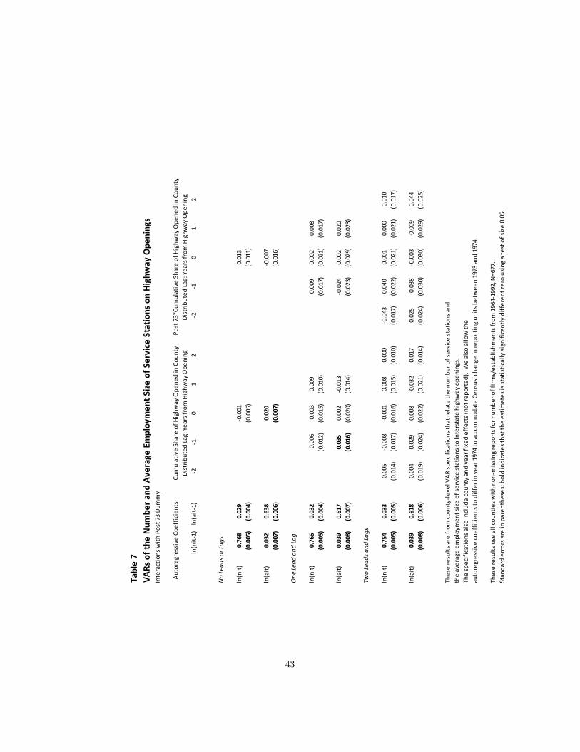
Tabl

e 7

VARs

 of t

he N

umbe

r and

 Ave

rage

 Em

ploy

men

t Size

 of S

ervi

ce S

tatio

ns o

n Hi

ghw

ay O

peni

ngs

Inte

ract

ions

 with

 Pos

t 73 

Dum

my

ln(n

it­1)

ln(a

it­1)

­2­1

01

2­2

­10

12

No 

Lead

s or L

ags

ln(n

it)0.

768

0.02

9­0

.001

0.01

3(0

.005

)(0

.004

)(0

.005

)(0

.011

)

ln(a

it)0.

032

0.63

80.

020

­0.0

07(0

.007

)(0

.006

)(0

.007

)(0

.016

)

One

 Lead

 and

 Lag

ln(n

it)0.

766

0.03

2­0

.006

­0.0

030.

009

0.00

90.

002

0.00

8(0

.005

)(0

.004

)(0

.012

)(0

.015

)(0

.010

)(0

.017

)(0

.021

)(0

.017

)

ln(a

it)0.

039

0.61

70.

035

0.00

2­0

.013

­0.0

240.

002

0.02

0(0

.008

)(0

.007

)(0

.016

)(0

.020

)(0

.014

)(0

.023

)(0

.029

)(0

.023

)

Two 

Lead

s and

 Lags

ln(n

it)0.

754

0.03

30.

005

­0.0

08­0

.001

0.00

80.

000

­0.0

430.

040

0.00

10.

000

0.01

0(0

.005

)(0

.005

)(0

.014

)(0

.017

)(0

.016

)(0

.015

)(0

.010

)(0

.017

)(0

.022

)(0

.021

)(0

.021

)(0

.017

)

ln(a

it)0.

039

0.61

80.

004

0.02

90.

008

­0.0

320.

017

0.02

5­0

.038

­0.0

03­0

.009

0.04

4(0

.008

)(0

.006

)(0

.019

)(0

.024

)(0

.022

)(0

.021

)(0

.014

)(0

.024

)(0

.030

)(0

.030

)(0

.029

)(0

.025

)

Thes

e re

sults

 are

 from

 coun

ty­le

vel V

AR sp

ecifi

catio

ns th

at re

late

 the 

num

ber o

f ser

vice

 stat

ions

 and

the 

aver

age 

empl

oym

ent s

ize 

of se

rvic

e st

atio

ns to

 Inte

rsta

te h

ighw

ay o

peni

ngs.

The 

spec

ifica

tions

 als

o in

clud

e co

unty

 and

 yea

r fix

ed e

ffec

ts (n

ot re

port

ed). 

 We 

also

 allo

w th

eau

tore

gres

sive

 coef

ficie

nts t

o di

ffer

 in y

ear 1

974 

to a

ccom

mod

ate 

Cens

us' c

hang

e in

 repo

rtin

g un

its b

etw

een 

1973

 and

 197

4.

Thes

e re

sults

 use

 all 

coun

ties w

ith n

on­m

issi

ng re

port

s for

 num

ber o

f firm

s/es

tabl

ishm

ents

 from

 196

4­19

92, N

=677

.St

anda

rd e

rror

s are

 in p

aren

thes

es; b

old 

indi

cate

s tha

t the

 est

imat

es is

 stat

istic

ally

 sign

ifica

ntly

 diff

eren

t zer

o us

ing 

a te

st o

f siz

e 0.

05.

Auto

regr

essi

ve C

oeff

icie

nts

Dist

ribut

ed La

g: Y

ears

 from

 Hig

hway

 Ope

ning

Post

 73*

Cum

ulat

ive 

Shar

e of

 Hig

hway

 Ope

ned 

in C

ount

yCu

mul

ativ

e Sh

are 

of H

ighw

ay O

pene

d in

 Cou

nty

Dist

ribut

ed La

g: Y

ears

 from

 Hig

hway

 Ope

ning

43

Tabl

e 9

VARs

 of t

he N

umbe

r and

 Ave

rage

 Em

ploy

men

t Size

 of S

ervi

ce S

tatio

ns o

n Hi

ghw

ay O

peni

ngs

Dist

ance

 Inte

ract

ions

, Tw

o Le

ads a

nd La

gs

ln(n

it­1)

ln(a

it­1)

­2­1

01

2­2

­10

12

d=0

d=10

No 

Lead

s or L

ags

ln(n

it)0.

768

0.03

0­0

.006

0.00

3­0

.005

0.02

1(0

.005

)(0

.004

)(0

.006

)(0

.001

)(0

.006

)(0

.010

)

ln(a

it)0.

039

0.61

70.

020

0.00

00.

020

0.01

8(0

.008

)(0

.007

)(0

.009

)(0

.002

)(0

.009

)(0

.014

)

One

 Lead

 and

 Lag

ln(n

it)0.

765

0.03

2­0

.010

0.00

7­0

.005

0.00

1­0

.003

0.00

5­0

.007

0.02

4(0

.005

)(0

.004

)(0

.015

)(0

.018

)(0

.013

)(0

.003

)(0

.005

)(0

.002

)(0

.007

)(0

.011

)

ln(a

it)0.

039

0.61

70.

054

­0.0

16­0

.011

­0.0

080.

006

0.00

00.

028

0.01

0(0

.008

)(0

.007

)(0

.020

)(0

.026

)(0

.017

)(0

.005

)(0

.005

)(0

.003

)(0

.010

)(0

.015

)

Two 

Lead

s and

 Lags

ln(n

it)0.

754

0.03

3­0

.010

­0.0

100.

016

­0.0

10­0

.003

0.00

00.

001

­0.0

050.

006

0.00

1­0

.008

0.02

4(0

.005

)(0

.005

)(0

.017

)(0

.021

)(0

.020

)(0

.188

)(0

.013

)(0

.004

)(0

.005

)(0

.004

)(0

.004

)(0

.003

)(0

.009

)(0

.013

)

ln(a

it)0.

039

0.61

70.

025

0.03

8­0

.011

­0.0

280.

010

­0.0

05­0

.007

0.00

6­0

.002

0.00

50.

035

0.00

5(0

.008

)(0

.007

)(0

.024

)(0

.030

)(0

.028

)(0

.026

)(0

.018

)(0

.005

)(0

.006

)(0

.006

)(0

.005

)(0

.003

)(0

.012

)(0

.018

)

Thes

e re

sults

 are

 from

 coun

ty­le

vel V

AR sp

ecifi

catio

ns th

at re

late

 the 

num

ber o

f ser

vice

 stat

ions

 and

the 

aver

age 

empl

oym

ent s

ize 

of se

rvic

e st

atio

ns to

 Inte

rsta

te h

ighw

ay o

peni

ngs.

The 

spec

ifica

tions

 als

o in

clud

e co

unty

 and

 yea

r fix

ed e

ffec

ts (n

ot re

port

ed). 

 We 

also

 allo

w th

eau

tore

gres

sive

 coef

ficie

nts t

o di

ffer

 in y

ear 1

974 

to a

ccom

mod

ate 

Cens

us' c

hang

e in

 repo

rtin

g un

its b

etw

een 

1973

 and

 197

4.

Thes

e re

sults

 use

 all 

coun

ties w

ith n

on­m

issi

ng re

port

s for

 num

ber o

f firm

s/es

tabl

ishm

ents

 from

 196

4­19

92, N

=677

.St

anda

rd e

rror

s are

 in p

aren

thes

es; b

old 

indi

cate

s tha

t the

 est

imat

es is

 stat

istic

ally

 sign

ifica

ntly

 diff

eren

t zer

o us

ing 

a te

st o

f siz

e 0.

05.

Auto

regr

essi

ve C

oeff

icie

nts

Dist

ribut

ed La

g: Y

ears

 from

 Hig

hway

 Ope

ning

Dist

ance

*Cum

ulat

ive 

Shar

e of

 Hig

hway

 Ope

ned 

in C

ount

ySu

m o

fLa

g Co

effic

ient

sCu

mul

ativ

e Sh

are 

of H

ighw

ay O

pene

d in

 Cou

nty

Dist

ribut

ed La

g: Y

ears

 from

 Hig

hway

 Ope

ning

44

Table 8Interaction Specifications with Distance From Old Route: No Leads or Lags

Dependent Variable: ln(nit)

CSMI 0.002 ­0.006 ­0.013(0.005) (0.006) (0.008)

CSMI*distance from old route 0.0027 0.0076(0.0012) (0.0035)

CSMI*(distance from old route)^2 ­0.0004(0.0002)

Dependent Variable: ln(ait)

CSMI 0.019 0.019 0.016(0.007) (0.008) (0.011)

CSMI*distance from old route ­0.0002 0.0022(0.0017) (0.0049)

CSMI*(distance from old route)^2 ­0.0002(0.0003)

These results are from county­level interactions that relate the number of service stationsand the average employment size of service stations to interstate highway openings.

The first column is the same as the top panel of Table 4.  The second and third interact the cumulative share ofhighway opened in the county (CSMI) with the average distance between the interstate and the old routethat it replaced in the county.

45

Number of Service Stations andYear From Interstate Highway Opening

­0.04

­0.02

0

0.02

0.04

0.06

0.08

0.1

­2 ­1 0 1 2 3 4 5 6

0 miles 1.25 miles 10 miles

Average Service Station Employment Size andYear From Interstate Highway Opening

­0.04

­0.02

0

0.02

0.04

0.06

0.08

0.1

­2 ­1 0 1 2 3 4 5 6

0 miles 1.25 miles 10 miles

Figure 5. Impulse-Response Functions for Highway Openings onMarket Structure of Service Stations, by Distance from Old Route.These graphs depict how the number and average size of service stations changearound the time that Interstate Highway segments are completed in a county,and how this di¤ers with how close the Interstate is from the previous route.The vertical axes scaled in log-points; 0.04 represents a 4% increase. Thehorizontal axis is years from segment completion; "-2" means two years beforea segment is completed. These graphs illustrate that when the Interstate wasclose to the old route, the industry adjustment was in an increase in average sta-tion size during the two years preceding the new highway�s completion. Whenit was far, the adjustment was an increase in the number of stations that tookplace after the new highway was completed.

46

47

Tabl

e 10

VARs

 of t

he N

umbe

r and

 Ave

rage

 Em

ploy

men

t Size

 of S

ervi

ce S

tatio

ns o

n Hi

ghw

ay O

peni

ngs

Dist

ance

 Inte

ract

ions

, One

 Lead

 and

 Lag

ln(n

it­1)

ln(a

it­1)

­10

1­1

01

­10

1d=

0d=

10

No 

Lead

s or L

ags

ln(n

it)0.

768

0.03

00.

005

­0.0

080.

003

0.00

50.

019

(0.0

05)

(0.0

04)

(0.0

10)

(0.0

07)

(0.0

01)

(0.0

10)

(0.0

10)

ln(a

it)0.

031

0.63

70.

014

0.01

60.

000

0.01

60.

012

(0.0

07)

(0.0

06)

(0.0

14)

(0.0

10)

(0.0

02)

(0.0

10)

(0.0

15)

One

 Lead

 and

 Lag

ln(n

it)0.

765

0.03

2­0

.025

0.00

90.

011

­0.0

060.

009

­0.0

080.

001

­0.0

020.

005

­0.0

040.

026

(0.0

05)

(0.0

04)

(0.0

19)

(0.0

22)

(0.0

16)

(0.0

15)

(0.0

19)

(0.0

13)

(0.0

03)

(0.0

04)

(0.0

02)

(0.0

08)

(0.0

12)

ln(a

it)0.

034

0.63

40.

001

0.00

90.

009

0.05

2­0

.013

­0.0

19­0

.008

0.00

60.

000

0.02

10.

001

(0.0

07)

(0.0

06)

(0.0

27)

(0.0

31)

(0.0

23)

(0.0

20)

(0.0

26)

(0.0

18)

(0.0

05)

(0.0

06)

(0.0

03)

(0.0

12)

(0.0

16)

Thes

e re

sults

 are

 from

 coun

ty­le

vel V

AR sp

ecifi

catio

ns th

at re

late

 the 

num

ber o

f ser

vice

 stat

ions

 and

the 

aver

age 

empl

oym

ent s

ize 

of se

rvic

e st

atio

ns to

 Inte

rsta

te h

ighw

ay o

peni

ngs.

The 

spec

ifica

tions

 als

o in

clud

e co

unty

 and

 yea

r fix

ed e

ffec

ts (n

ot re

port

ed). 

 We 

also

 allo

w th

eau

tore

gres

sive

 coef

ficie

nts t

o di

ffer

 in y

ear 1

974 

to a

ccom

mod

ate 

Cens

us' c

hang

e in

 repo

rtin

g un

its b

etw

een 

1973

 and

 197

4.

Thes

e re

sults

 use

 all 

coun

ties w

ith n

on­m

issi

ng re

port

s for

 num

ber o

f firm

s/es

tabl

ishm

ents

 from

 196

4­19

92, N

=677

.St

anda

rd e

rror

s are

 in p

aren

thes

es; b

old 

indi

cate

s tha

t the

 est

imat

es is

 stat

istic

ally

 sign

ifica

ntly

 diff

eren

t zer

o us

ing 

a te

st o

f siz

e 0.

05.

Auto

regr

essi

ve C

oeff

icie

nts

Ope

ned 

in C

ount

y*Di

stan

ceSu

m o

fLa

g Co

effic

ient

sCu

mul

ativ

e Sh

are 

of H

ighw

ayO

pene

d in

 Cou

nty

Cum

ulat

ive 

Shar

e of

 Hig

hway

Ope

ned 

in C

orrid

orCu

mul

ativ

e Sh

are 

of H

ighw

ay

48

Table 11VARs of the Number and Average Employment Size of Service Stations on Highway OpeningsDistance Interactions, One Lead and Lag

ln(nit­1) ln(ait­1) ­1 0 1 ­1 0 1 d=0 d=10

No Leads or Lags

ln(nit) 0.766 0.029 0.017 0.005 0.017 0.071(0.005) (0.004) (0.012) (0.003) (0.012) (0.020)

ln(ait) 0.030 0.636 0.067 ­0.005 0.067 0.019(0.007) (0.006) (0.017) (0.004) (0.017) (0.028)

ln(nit) ­0.034 ­0.001 ­0.034 ­0.044(0.015) (0.003) (0.015) (0.026)

ln(ait) ­0.037 0.006 ­0.037 0.019(0.020) (0.005) (0.020) (0.035)

One Lead and Lag

ln(nit) 0.764 0.032 0.011 ­0.020 0.029 0.003 ­0.001 0.004 0.019 0.079(0.005) (0.004) (0.030) (0.039) (0.026) (0.007) (0.008) (0.005) (0.014) (0.022)

ln(ait) 0.032 0.633 0.077 ­0.023 0.024 ­0.023 0.012 0.002 0.077 ­0.016(0.007) (0.006) (0.042) (0.054) 0.036 (0.009) (0.010) (0.007) (0.018) (0.031)

ln(nit) ­0.030 0.038 ­0.046 ­0.003 ­0.004 0.005 ­0.038 ­0.049(0.038) (0.049) (0.033) (0.009) (0.011) (0.007) (0.016) (0.028)

ln(ait) 0.018 0.004 ­0.057 0.014 ­0.003 ­0.003 ­0.036 0.044(0.053) (0.068) (0.046) (0.012) (0.015) (0.011) (0.023) (0.039)

These results are from county­level VAR specifications that relate the number of service stations andthe average employment size of service stations to Interstate highway openings.The specifications also include county and year fixed effects (not reported).  We also allow theautoregressive coefficients to differ in year 1974 to accommodate Census' change in reporting units between 1973 and 1974.

These results use all counties with non­missing reports for number of firms/establishments from 1964­1992, N=677.Standard errors are in parentheses; bold indicates that the estimates is statistically significantly different zero using a test of size 0.05.

Opened in County Opened in County*Distance CountyAutoregressive Coefficients Cumulative Share of Highway Cumulative Share of Highway Sum of Dist. Lags:

Interactions with (1­"thrushare")

Interactions with "thrushare"

Interactions with "thrushare"

Interactions with (1­"thrushare")

49

Table A1Cities that Are Corridor Endpoints

Abilene, TX Detroit, MI Madison, WI San Bernardino, CAAkron, OH Durham, NC Memphis, TN San Diego, CAAlbany, NY El Paso, TX Miami, FL San Francisco, CAAlbuquerque, NM Erie, PA Milwaukee, WI Savannah, GAAllentown, PA Eugene, OR Minneapolis, MN Seattle, WAAmarillo, TX Flint, MI Mobile, AL Shreveport, LAAnn Arbor, MI Fort Lauderdale, FL Montgomery, AL Sioux Falls, SDAtlanta, GA Fort Wayne, IN Nashville, TN South Bend, INAustin, TX Fort Worth, TX New Haven, CT Spokane, WABaltimore, MD Gary, IN New Orleans, LA Springfield, ILBaton Rouge, LA Grand Rapids, MI New York, NY Springfield, MOBeaumont, TX Greensboro, NC Newark, NJ St. Louis, MOBirmingham, AL Hartford, CT Norfolk, VA Stockton, CABoise, ID Houston, TX Oklahoma City, OK Syracuse, NYBoston, MA Indianapolis, IN Omaha, NE Tacoma, WABridgeport, CT Jackson, MS Orlando, FL Tallahassee, FLBuffalo, NY Jacksonville, FL Peoria, IL Tampa, FLCharlotte, NC Kansas City, MO Philadelphia, PA Toledo, OHChattanooga, TN Knoxville, TN Phoenix, AZ Topeka, KSChicago, IL Lafayette, LA Pittsburgh, PA Tucson, AZCincinnati, OH Lansing, MI Portland, OR Tulsa, OKCleveland, OH Laredo, TX Providence, RI Waco, TXColorado Springs, CO Las Vegas, NV Raleigh, NC Washington, DCColumbia, SC Lexington, KY Reno, NV Wichita, KSColumbus, OH Lincoln, NE Richmond, VA Winston Salem, NCCorpus Christi, TX Little Rock, AR Rockford, ILDallas, TX Los Angeles, CA Sacramento, CADayton, OH Louisville, KY Salem, ORDenver, CO Lubbock, TX Salt Lake City, UTDes Moines, IA Macon, GA San Antonio, TX

50

51

Tabl

e A2

VARs

 of t

he N

umbe

r and

 Ave

rage

 Em

ploy

men

t Size

 of S

ervi

ce S

tatio

ns o

n Hi

ghw

ay O

peni

ngs

Dist

ance

 Inte

ract

ions

, Inc

lude

s Onl

y Co

untie

s Whe

re D

ista

nce 

From

 Old

 Rou

te Is

 Gre

ater

 Tha

n 1/

2 M

ile

ln(n

it­1)

ln(a

it­1)

­2­1

01

2­2

­10

12

d=0

d=10

No 

Lead

s or L

ags

ln(n

it)0.

767

0.03

2­0

.006

0.00

2­0

.006

0.01

8(0

.006

)(0

.005

)(0

.007

)(0

.001

)(0

.007

)(0

.010

)

ln(a

it)0.

027

0.63

50.

020

­0.0

010.

020

0.01

3(0

.008

)(0

.007

)(0

.010

)(0

.001

)(0

.010

)(0

.014

)

One

 Lead

 and

 Lag

ln(n

it)0.

766

0.03

5­0

.018

0.02

5­0

.014

0.00

2­0

.006

0.00

6­0

.007

0.02

0(0

.006

)(0

.005

)(0

.017

)(0

.021

)(0

.014

)(0

.003

)(0

.004

)(0

.003

)(0

.008

)(0

.011

)

ln(a

it)0.

030

0.63

20.

060

­0.0

14­0

.019

­0.0

090.

006

0.00

10.

026

0.00

3(0

.008

)(0

.007

)(0

.023

)(0

.030

)(0

.020

)(0

.005

)(0

.006

)(0

.003

)(0

.011

)(0

.015

)

Thes

e re

sults

 are

 from

 coun

ty­le

vel V

AR sp

ecifi

catio

ns th

at re

late

 the 

num

ber o

f ser

vice

 stat

ions

 and

the 

aver

age 

empl

oym

ent s

ize 

of se

rvic

e st

atio

ns to

 Inte

rsta

te h

ighw

ay o

peni

ngs.

The 

spec

ifica

tions

 als

o in

clud

e co

unty

 and

 yea

r fix

ed e

ffec

ts (n

ot re

port

ed). 

 We 

also

 allo

w th

eau

tore

gres

sive

 coef

ficie

nts t

o di

ffer

 in y

ear 1

974 

to a

ccom

mod

ate 

Cens

us' c

hang

e in

 repo

rtin

g un

its b

etw

een 

1973

 and

 197

4.

Thes

e re

sults

 use

 all 

coun

ties w

ith n

on­m

issi

ng re

port

s for

 num

ber o

f firm

s/es

tabl

ishm

ents

 from

 196

4­19

92, a

nd fo

r whi

ch d

ista

nce 

from

 old

 rout

e > 

1/2 

mile

, N=5

18.

Stan

dard

 err

ors a

re in

 par

enth

eses

; bol

d in

dica

tes t

hat t

he e

stim

ates

 is st

atis

tical

ly si

gnifi

cant

ly d

iffer

ent z

ero 

usin

g a 

test

 of s

ize 

0.05

.

Auto

regr

essi

ve C

oeff

icie

nts

Dist

ribut

ed La

g: Y

ears

 from

 Hig

hway

 Ope

ning

Dist

ance

*Cum

ulat

ive 

Shar

e of

 Hig

hway

 Ope

ned 

in C

ount

ySu

m o

fLa

g Co

effic

ient

sCu

mul

ativ

e Sh

are 

of H

ighw

ay O

pene

d in

 Cou

nty

Dist

ribut

ed La

g: Y

ears

 from

 Hig

hway

 Ope

ning

52

1

Working Paper Series

A series of research studies on regional economic issues relating to the Seventh Federal Reserve District, and on financial and economic topics.

U.S. Corporate and Bank Insolvency Regimes: An Economic Comparison and Evaluation WP-06-01 Robert R. Bliss and George G. Kaufman

Redistribution, Taxes, and the Median Voter WP-06-02 Marco Bassetto and Jess Benhabib

Identification of Search Models with Initial Condition Problems WP-06-03 Gadi Barlevy and H. N. Nagaraja

Tax Riots WP-06-04 Marco Bassetto and Christopher Phelan

The Tradeoff between Mortgage Prepayments and Tax-Deferred Retirement Savings WP-06-05 Gene Amromin, Jennifer Huang,and Clemens Sialm

Why are safeguards needed in a trade agreement? WP-06-06 Meredith A. Crowley

Taxation, Entrepreneurship, and Wealth WP-06-07 Marco Cagetti and Mariacristina De Nardi

A New Social Compact: How University Engagement Can Fuel Innovation WP-06-08 Laura Melle, Larry Isaak, and Richard Mattoon

Mergers and Risk WP-06-09 Craig H. Furfine and Richard J. Rosen

Two Flaws in Business Cycle Accounting WP-06-10 Lawrence J. Christiano and Joshua M. Davis

Do Consumers Choose the Right Credit Contracts? WP-06-11 Sumit Agarwal, Souphala Chomsisengphet, Chunlin Liu, and Nicholas S. Souleles

Chronicles of a Deflation Unforetold WP-06-12 François R. Velde

Female Offenders Use of Social Welfare Programs Before and After Jail and Prison: Does Prison Cause Welfare Dependency? WP-06-13 Kristin F. Butcher and Robert J. LaLonde

Eat or Be Eaten: A Theory of Mergers and Firm Size WP-06-14 Gary Gorton, Matthias Kahl, and Richard Rosen

2

Working Paper Series (continued) Do Bonds Span Volatility Risk in the U.S. Treasury Market? A Specification Test for Affine Term Structure Models WP-06-15 Torben G. Andersen and Luca Benzoni Transforming Payment Choices by Doubling Fees on the Illinois Tollway WP-06-16 Gene Amromin, Carrie Jankowski, and Richard D. Porter

How Did the 2003 Dividend Tax Cut Affect Stock Prices? WP-06-17 Gene Amromin, Paul Harrison, and Steven Sharpe

Will Writing and Bequest Motives: Early 20th Century Irish Evidence WP-06-18 Leslie McGranahan

How Professional Forecasters View Shocks to GDP WP-06-19 Spencer D. Krane

Evolving Agglomeration in the U.S. auto supplier industry WP-06-20 Thomas Klier and Daniel P. McMillen

Mortality, Mass-Layoffs, and Career Outcomes: An Analysis using Administrative Data WP-06-21 Daniel Sullivan and Till von Wachter

The Agreement on Subsidies and Countervailing Measures: Tying One’s Hand through the WTO. WP-06-22 Meredith A. Crowley

How Did Schooling Laws Improve Long-Term Health and Lower Mortality? WP-06-23 Bhashkar Mazumder

Manufacturing Plants’ Use of Temporary Workers: An Analysis Using Census Micro Data WP-06-24 Yukako Ono and Daniel Sullivan

What Can We Learn about Financial Access from U.S. Immigrants? WP-06-25 Una Okonkwo Osili and Anna Paulson

Bank Imputed Interest Rates: Unbiased Estimates of Offered Rates? WP-06-26 Evren Ors and Tara Rice

Welfare Implications of the Transition to High Household Debt WP-06-27 Jeffrey R. Campbell and Zvi Hercowitz

Last-In First-Out Oligopoly Dynamics WP-06-28 Jaap H. Abbring and Jeffrey R. Campbell

Oligopoly Dynamics with Barriers to Entry WP-06-29 Jaap H. Abbring and Jeffrey R. Campbell

Risk Taking and the Quality of Informal Insurance: Gambling and Remittances in Thailand WP-07-01 Douglas L. Miller and Anna L. Paulson

3

Working Paper Series (continued) Fast Micro and Slow Macro: Can Aggregation Explain the Persistence of Inflation? WP-07-02 Filippo Altissimo, Benoît Mojon, and Paolo Zaffaroni

Assessing a Decade of Interstate Bank Branching WP-07-03 Christian Johnson and Tara Rice

Debit Card and Cash Usage: A Cross-Country Analysis WP-07-04 Gene Amromin and Sujit Chakravorti

The Age of Reason: Financial Decisions Over the Lifecycle WP-07-05 Sumit Agarwal, John C. Driscoll, Xavier Gabaix, and David Laibson

Information Acquisition in Financial Markets: a Correction WP-07-06 Gadi Barlevy and Pietro Veronesi

Monetary Policy, Output Composition and the Great Moderation WP-07-07 Benoît Mojon

Estate Taxation, Entrepreneurship, and Wealth WP-07-08 Marco Cagetti and Mariacristina De Nardi

Conflict of Interest and Certification in the U.S. IPO Market WP-07-09 Luca Benzoni and Carola Schenone

The Reaction of Consumer Spending and Debt to Tax Rebates – Evidence from Consumer Credit Data WP-07-10 Sumit Agarwal, Chunlin Liu, and Nicholas S. Souleles

Portfolio Choice over the Life-Cycle when the Stock and Labor Markets are Cointegrated WP-07-11 Luca Benzoni, Pierre Collin-Dufresne, and Robert S. Goldstein Nonparametric Analysis of Intergenerational Income Mobility WP-07-12

with Application to the United States Debopam Bhattacharya and Bhashkar Mazumder

How the Credit Channel Works: Differentiating the Bank Lending Channel WP-07-13

and the Balance Sheet Channel Lamont K. Black and Richard J. Rosen

Labor Market Transitions and Self-Employment WP-07-14

Ellen R. Rissman

First-Time Home Buyers and Residential Investment Volatility WP-07-15

Jonas D.M. Fisher and Martin Gervais

Establishments Dynamics and Matching Frictions in Classical Competitive Equilibrium WP-07-16

Marcelo Veracierto

Technology’s Edge: The Educational Benefits of Computer-Aided Instruction WP-07-17

Lisa Barrow, Lisa Markman, and Cecilia Elena Rouse

4

Working Paper Series (continued) The Widow’s Offering: Inheritance, Family Structure, and the Charitable Gifts of Women WP-07-18

Leslie McGranahan

Demand Volatility and the Lag between the Growth of Temporary and Permanent Employment WP-07-19

Sainan Jin, Yukako Ono, and Qinghua Zhang

A Conversation with 590 Nascent Entrepreneurs WP-07-20

Jeffrey R. Campbell and Mariacristina De Nardi

Cyclical Dumping and US Antidumping Protection: 1980-2001 WP-07-21

Meredith A. Crowley

Health Capital and the Prenatal Environment: The Effect of Maternal Fasting During Pregnancy WP-07-22

Douglas Almond and Bhashkar Mazumder

The Spending and Debt Response to Minimum Wage Hikes WP-07-23

Daniel Aaronson, Sumit Agarwal, and Eric French

The Impact of Mexican Immigrants on U.S. Wage Structure WP-07-24

Maude Toussaint-Comeau

A Leverage-based Model of Speculative Bubbles WP-08-01

Gadi Barlevy

Displacement, Asymmetric Information and Heterogeneous Human Capital WP-08-02

Luojia Hu and Christopher Taber

BankCaR (Bank Capital-at-Risk): A credit risk model for US commercial bank charge-offs WP-08-03

Jon Frye and Eduard Pelz

Bank Lending, Financing Constraints and SME Investment WP-08-04

Santiago Carbó-Valverde, Francisco Rodríguez-Fernández, and Gregory F. Udell

Global Inflation WP-08-05

Matteo Ciccarelli and Benoît Mojon

Scale and the Origins of Structural Change WP-08-06

Francisco J. Buera and Joseph P. Kaboski

Inventories, Lumpy Trade, and Large Devaluations WP-08-07

George Alessandria, Joseph P. Kaboski, and Virgiliu Midrigan

School Vouchers and Student Achievement: Recent Evidence, Remaining Questions WP-08-08

Cecilia Elena Rouse and Lisa Barrow

5

Working Paper Series (continued) Does It Pay to Read Your Junk Mail? Evidence of the Effect of Advertising on Home Equity Credit Choices WP-08-09

Sumit Agarwal and Brent W. Ambrose

The Choice between Arm’s-Length and Relationship Debt: Evidence from eLoans WP-08-10

Sumit Agarwal and Robert Hauswald

Consumer Choice and Merchant Acceptance of Payment Media WP-08-11

Wilko Bolt and Sujit Chakravorti Investment Shocks and Business Cycles WP-08-12

Alejandro Justiniano, Giorgio E. Primiceri, and Andrea Tambalotti New Vehicle Characteristics and the Cost of the Corporate Average Fuel Economy Standard WP-08-13

Thomas Klier and Joshua Linn

Realized Volatility WP-08-14

Torben G. Andersen and Luca Benzoni

Revenue Bubbles and Structural Deficits: What’s a state to do? WP-08-15

Richard Mattoon and Leslie McGranahan The role of lenders in the home price boom WP-08-16

Richard J. Rosen

Bank Crises and Investor Confidence WP-08-17

Una Okonkwo Osili and Anna Paulson Life Expectancy and Old Age Savings WP-08-18

Mariacristina De Nardi, Eric French, and John Bailey Jones Remittance Behavior among New U.S. Immigrants WP-08-19

Katherine Meckel Birth Cohort and the Black-White Achievement Gap: The Roles of Access and Health Soon After Birth WP-08-20

Kenneth Y. Chay, Jonathan Guryan, and Bhashkar Mazumder

Public Investment and Budget Rules for State vs. Local Governments WP-08-21

Marco Bassetto

Why Has Home Ownership Fallen Among the Young? WP-09-01

Jonas D.M. Fisher and Martin Gervais

Why do the Elderly Save? The Role of Medical Expenses WP-09-02

Mariacristina De Nardi, Eric French, and John Bailey Jones

Using Stock Returns to Identify Government Spending Shocks WP-09-03

Jonas D.M. Fisher and Ryan Peters

6

Working Paper Series (continued) Stochastic Volatility WP-09-04

Torben G. Andersen and Luca Benzoni The Effect of Disability Insurance Receipt on Labor Supply WP-09-05

Eric French and Jae Song CEO Overconfidence and Dividend Policy WP-09-06

Sanjay Deshmukh, Anand M. Goel, and Keith M. Howe Do Financial Counseling Mandates Improve Mortgage Choice and Performance? WP-09-07 Evidence from a Legislative Experiment

Sumit Agarwal,Gene Amromin, Itzhak Ben-David, Souphala Chomsisengphet, and Douglas D. Evanoff Perverse Incentives at the Banks? Evidence from a Natural Experiment WP-09-08

Sumit Agarwal and Faye H. Wang Pay for Percentile WP-09-09

Gadi Barlevy and Derek Neal

The Life and Times of Nicolas Dutot WP-09-10

François R. Velde

Regulating Two-Sided Markets: An Empirical Investigation WP-09-11

Santiago Carbó Valverde, Sujit Chakravorti, and Francisco Rodriguez Fernandez

The Case of the Undying Debt WP-09-12

François R. Velde

Paying for Performance: The Education Impacts of a Community College Scholarship Program for Low-income Adults WP-09-13

Lisa Barrow, Lashawn Richburg-Hayes, Cecilia Elena Rouse, and Thomas Brock

Establishments Dynamics, Vacancies and Unemployment: A Neoclassical Synthesis WP-09-14

Marcelo Veracierto

The Price of Gasoline and the Demand for Fuel Economy: Evidence from Monthly New Vehicles Sales Data WP-09-15

Thomas Klier and Joshua Linn

Estimation of a Transformation Model with Truncation, Interval Observation and Time-Varying Covariates WP-09-16

Bo E. Honoré and Luojia Hu

Self-Enforcing Trade Agreements: Evidence from Antidumping Policy WP-09-17

Chad P. Bown and Meredith A. Crowley

Too much right can make a wrong: Setting the stage for the financial crisis WP-09-18

Richard J. Rosen Can Structural Small Open Economy Models Account for the Influence of Foreign Disturbances? WP-09-19

Alejandro Justiniano and Bruce Preston

7

Working Paper Series (continued) Liquidity Constraints of the Middle Class WP-09-20

Jeffrey R. Campbell and Zvi Hercowitz

Monetary Policy and Uncertainty in an Empirical Small Open Economy Model WP-09-21

Alejandro Justiniano and Bruce Preston

Firm boundaries and buyer-supplier match in market transaction: IT system procurement of U.S. credit unions WP-09-22

Yukako Ono and Junichi Suzuki

Health and the Savings of Insured Versus Uninsured, Working-Age Households in the U.S. WP-09-23

Maude Toussaint-Comeau and Jonathan Hartley

The Economics of “Radiator Springs:” Industry Dynamics, Sunk Costs, and Spatial Demand Shifts WP-09-24

Jeffrey R. Campbell and Thomas N. Hubbard