The Economics of Missionary Expansion:

Evidence from Africa and Implications for Development

Remi Jedwab and Felix Meier zu Selhausen and Alexander Moradi*

June 25, 2021

Abstract

How did Christianity expand in Africa to become the continent’s dominant religion?

Using annual panel census data on Christian missions from 1751 to 1932 in Ghana,

and pre-1924 data on missions for 43 sub-Saharan African countries, we estimate causal

effects of malaria, railroads and cash crops on mission location. We find that missions

were established in healthier, more accessible, and richer places before expanding to

economically less developed places. We argue that the endogeneity of missionary

expansion may have been underestimated, thus questioning the link between missions

and economic development for Africa. We find the endogeneity problem exacerbated

when mission data is sourced from Christian missionary atlases that disproportionately

report a selection of prominent missions that were also established early.

JEL Codes: O10, O40, Z12, I20, N30

Keywords: Economics of Religion; Religious Diffusion; Human Capital; Economic

Persistence; Measurement; Historical Data; Atlases; Missions; Christianity; Africa

*Corresponding author: Alexander Moradi: Free University of Bozen-Bolzano, Department of Economics, Alexan-der.Moradi@unibz.it. Remi Jedwab: George Washington University, Department of Economics, jedwab@gwu.edu.Felix Meier zu Selhausen: Wageningen University, felix.meierzuselhausen@wur.nl. We gratefully thank Oded Galor,three anonymous referees, Robert Barro, Sascha Becker, James Fenske, Ewout Frankema, Laurence Iannaccone, TimurKuran, Stelios Michalopoulos, Dozie Okoye, Elias Papaioannou, Jared Rubin, Felipe Valencia Caicedo and LeonardWantchekon for their helpful comments. We are grateful to seminar audiences at AEHN (Wageningen, Sussex), ASREC(Bologna, Luxembourg), Belfast, Bocconi, Bolzano, CEPR Economics of Religion (Venice), CSAE (Oxford), Dalhousie,EHES (Tubingen), EHS (Keele), GDE (Zurich), George Mason, George Washington, Frankfurt, Gottingen, Ingolstadt,Munich, Namur, Passau, Stellenbosch, Sussex, Tubingen, Utrecht, Warwick and WEHC (Boston). We thank NathanNunn, Julia Cage and Valeria Rueda, and Morgan Henderson and Warren Whatley, for sharing their datasets. Wethank Madeline De Quillacq for excellent research assistance. Meier zu Selhausen gratefully acknowledges financialsupport of the British Academy (Postdoctoral Fellowship no. pf160051 - Conversion out of Poverty? Exploring theOrigins and Long-Term Consequences of Christian Missionary Activities in Africa).

1

One of the most powerful cultural transformations in modern history has been the rapid

expansion of Christianity to regions outside Europe. Conversion has been markedly rapid in

sub-Saharan Africa. While Christians made up about 5% of the population in 1900, their share

has grown to 57% today (Johnson and Grim, 2020), making Africa the continent with the highest

number of Christians (Todd et al., 2018). At current trends, Africans will comprise 42% of the

global Christian population by 2060. According to the World Values Survey, sub-Saharan Africa is

also home to the world’s most observant Christians in terms of church attendance, making it “the

future of the world’s most popular religion” (The Economist, 2015).

The process of African mass-conversion was facilitated by vast Christian missionary efforts.

Throughout the colonial era missions provided the bulk of formal education (Frankema, 2012;

Cogneau and Moradi, 2014) and health care (Doyle et al., 2020). A recent and rapidly growing

literature explores the long-term effects of missions in colonial Africa, as well as in India and

Latin America. Web Appx. Table A1 summarizes 50 studies that find strong effects on local

economic development (Bai and Kung, 2015; Castello-Climent et al., 2018; Valencia Caicedo,

2019a), education (Gallego and Woodberry, 2010; Acemoglu et al., 2014; Waldinger, 2017; Calvi et

al., 2021), health (Calvi and Mantovanelli, 2018; Cage and Rueda, 2020; Menon and McQueeney,

2020), social mobility (Wantchekon et al., 2015; Alesina et al., 2019), culture (Nunn, 2010, 2014;

Fenske, 2015; Calvi et al., 2021), and political participation (Cage and Rueda, 2016).1

While a large literature has studied the economic consequences of evangelization, the economics

behind the expansion of Christianity remains poorly understood. One narrative describes

missionaries as adventurers, with little to no information on local circumstances, crossing political

boundaries and whose objective was to save souls no matter the cost (Oliver, 1952; Cleall, 2009).

Their locational choices were highly erratic, but once settled, missions persisted. For example,

Wantchekon et al. (2015, p. 714) describes how a series of historical accidents led missionaries

to settle left rather than right of a river. An alternative view is that missionaries were following

clear expansion strategies laid out by their own mission society (Johnson, 1967; Terry, 2015). For

example, missionary Thauren (1931, pp. 19-20) described the strategy in Togo as follows:

“The mission leadership knew that choosing suitable places would be crucial for

missionizing the interior. Therefore, no effort was spared to get to know the interior

better [...]. The mission society aimed to establish new stations in larger cities, so that

1See Valencia Caicedo (2019b) and Meier zu Selhausen (2019) for surveys of the literature on missionary legacies.

2

few missionaries could spread the gospel to many. In particular, they preferred cities

with regular markets. Moreover, the places needed to be centrally located [...].”

Missions also aimed for financial independence, which would make them target wealthy loca-

tions. To our knowledge, the causal determinants of mission expansion have not been studied.2

In this paper, we study the determinants and effects of missionary expansion in Ghana and sub-

Saharan Africa as a whole. For various reasons, Ghana is an ideal testing ground. First, Ghana is

one of the most devout Christian African countries today.3 Second, Ghana received missionaries

since the early 19th century, which allows us to investigate the role of quinine as a groundbreaking

treatment for malaria ca. 1850. Missionary expansion in East Africa began later in the 1890s. Third,

in Ghana missionaries operated in a comparatively free religious market with little interference

by the colonial state (Gallego and Woodberry, 2010).4 Finally, Ghana holds rich historical data.

Altogether, this enables us to shed light on a wide range of determinants of mission expansion.

For Ghana, we create a novel annual panel dataset on the locations of missions at a precise

spatial level over two centuries: 2,091 grid cells of 0.1x0.1 degrees (12x12km) in 1751-1932, when

the number of missions increased from one to 1,832. Creating new data on the determinants

of mission locations, descriptive results suggest that missionaries might have gone to healthier,

more accessible, and richer areas, privileging these “better” locations first. They might also

have invested more into these missions/locations (with administrative functions, European

missionaries and schools). These results are confirmed using identification strategies for malaria,

railroads, and cash crops, in Ghana, but also in sub-Saharan Africa.

Once missionary expansion is better understood, we can study the long-term effects of missions.

With a few exceptions, existing studies do not analyze the effects of missions on economic

development per se, focus on one mechanism at a time, and, more importantly, use data from

mission atlases that are marred by omissions (see Web Appx. Table A1). Figure 1(a) plots the

mission locations obtained from the two most commonly used sources: (i) the Atlas of Protestant

Missions (Beach, 1903), first used by Cage and Rueda (2016), and (ii) the Ethnographic Survey of

Africa (Roome, 1925), digitized by Nunn (2010, 2014).5 Using ecclesiastical census returns and2Nunn (2010) and Cage and Rueda (2016) examine the effects of factors such as population density, urbanization,

railroads, explorer routes, malaria and slavery. However, their quantitative analyses are not dynamic, nor causal.3The Economist. True Believers: Christians in Ghana and Nigeria. September 5th 2012.4In contrast, Belgian, Portuguese and Spanish colonies granted Catholic missions a quasi-monopoly (Meier zu

Selhausen, 2019). French colonies followed from the 1890s on a more neutral treatment of missionaries in that theyrestricted most of the activities of both Catholics and Protestants (Sundkler and Steed, 2000, p. 430).

530 studies use Roome (1925), 6 studies use Beach (1903). Five use Bartholomew et al. (1911), and 6 use Streit (1913).

3

other primary sources instead, we uncover vast discrepancies. Figure 1(b) shows that atlases omit

more than 90% of missions in most African countries.6 Beach (1903) and Roome (1925) imply

congregation sizes of more than 3,000 and 15,000 per mission station respectively.7 For Ghana, the

two atlases miss 91-98% of missions, most of them in the hinterland (see Fig. 2(a)-2(b)). Our census

data suggest an average congregation size of 198 in 1925, which appears far more plausible.8

We discuss the implications of the observed patterns of missionary expansion and the over-

reliance on mission atlases for the study of the long-term effects of missions. We highlight three

sources of endogeneity: (i) attenuation bias, (ii) selection bias, and (iii) omitted variable bias.

First, we scrutinize the standard source of mission data. Atlases do not show the distribution of

the universe of missions. Classical measurement error would lead to attenuation bias. However,

measurement error may be non-classical, e.g. if omissions are not random. We use our census-

based data on Ghana to show that atlases positively select missions, in particular early, main or

European residence missions located in more developed areas. This would bias estimates upward.

Next, we examine whether the source of mission data affects the estimated long-term impact of

missions in Ghana. Employing the control variables commonly used in the literature on missions

in Africa (e.g., Nunn, 2010, 2014; Cage and Rueda, 2016), we find strong effects that are twice as

large for atlas missions than for census missions. If we use a rich and historically relevant set of

control variables, estimated effects are considerably weaker. This also applies to Africa as a whole.

Our interpretation is that mission atlases, because they report “better” missions endogenously

located in “better” places, may capture effects that are not due to the missions themselves.

Moreover, relying on atlases raises concerns of external validity. Estimated effects are measured

for a selected subset of missions that are not representative of the average mission. To

measure causal long-term effects of missions, one must properly control for the spatio-historical

determinants of missions, or use an identification strategy that can be implemented even with

imperfect historical controls. While a handful of studies have relied on innovative identification

strategies (e.g., Wantchekon et al., 2015; Cage and Rueda, 2016; Waldinger, 2017; Valencia Caicedo,

6Weighting the country-specific omission rates in Beach (1903) and Roome (1925) by the countries’ populationca. 1920 (Frankema and Jerven, 2014), we find for the whole of sub-Saharan Africa that 76% of Protestant missionsare missing from Beach (vs. 91% for Ghana) and 91% of them are missing from Roome (vs. 98% for Ghana).

7Beach (1903) and Roome (1925) report 677 Protestant and 1,212 Christian mission stations respectively. Accordingto the World Christian Database (Johnson and Zurlo, 2021), Protestants in 1900 numbered 2.2 million. For the year 1925,there were an estimated 20.2 million Christians in sub-Saharan Africa (excluding Ethiopia).

8Bartholomew et al. (1911) and Streit (1913) then miss circa 85-95% of missions in China, India, Korea, and Japan.

4

2019a)9, many studies use some controls and sometimes add spatial fixed effects.

Our contribution is threefold. First, our paper relates to the literature on the determinants of the

adoption and diffusion of religion (Bisin and Verdier, 2000; Barro and McCleary, 2005; McCleary

and Barro, 2006; Becker and Woessmann, 2013; Becker et al., 2017a). There are few quantitative

works on religious diffusion, and none for sub-Saharan Africa. Michalopoulos et al. (2018) pointed

to the role of geography and trade in the diffusion of Islam. Cantoni (2012) linked the spread

of Protestantism in 16th century Germany to strategic choices of territorial lords, while Rubin

(2014) shows that Protestantism followed cities’ adoption of the printing press. We show that in

Africa Christianity spread along railroads, with the cultivation of cash crops, and with economic

development more generally, before it diffused more broadly.

Second, our contribution is methodological. Non-classical measurement error in historical data

and their consequences for the analysis of path dependence are under-investigated. Measurement

error in survey data, in contrast, has received a lot of attention (e.g. Bollinger, 1996; Mahajan, 2006).

We emphasize the importance of: (i) reliable mission data, especially given external validity issues;

(ii) relevant controls capturing the dynamics and factors behind missionary expansion; and, when

needed, (iii) identification strategies that bypass issues related to these measurement issues.

Finally, we add to the literature on the long-term impact of missions.10 A large body of

literature has found positive effects on various proximate determinants of economic growth

(Web Appx. Table A1). Missions were the most important human capital promoting institutions

to have emerged in developing countries during the colonial era. By shaping attitudes towards

factors such as education and fertility, factors that alter the religious orientation of society may

have important repercussions for the growth process (Galor, 2011b; Becker et al., 2017b). With our

improved data we find comparably weaker long-term effects of missions in Ghana and Africa.11

9Wantchekon et al. (2015) rely on control villages that were as “as likely to be selected” as the villages with a mission.Cage and Rueda (2016) compare different types of investments between missions. Valencia Caicedo (2019a) andBergeron (2020) compare mission locations to places that missions abandoned for exogenous reasons. Valencia Caicedo(2019a) and Jedwab et al. (2021) compare locations exogenously evangelized by different denominations. Finally,Waldinger (2017) and Jedwab et al. (2021) exploit the initial directions of missionary expansion paths.

10For seminal studies on the impact of the Reformation, see Becker and Woessmann (2009); Becker et al. (2016).11Within the Unified Growth Theory (UGT) literature (see Galor (2005, 2011b) for surveys), various studies examine

how the emergence of human capital promoting institutions has affected the pace of the transition from stagnationto growth (Galor, 2011a). These studies have focused on the expansion of public schooling, such as the creationof a publicly supported secondary school system in the U.K. in 1902 (Galor and Moav, 2006) and the U.S. HighSchool Movement in the first half of the 20th century (Galor et al., 2009). The weak long-term economic effects ofcolonial missions in Africa could be due to African countries having not yet fully entered the process of human capitaldemanding “industrialization” (see, for example, Gollin et al. (2016)) that the UGT has shown to be the main driverbehind human capital formation and the demographic transition, and thus the transition to modern economic growth.

5

1. New Data on Ghana and Africa

To examine the determinants of missionary expansion, and draw implications for the analysis

of long-term development, we require data on the location of missions over time, the locational

factors potentially driving missions’ spatial expansion, and local economic development today.

The Web Appendix provides more details on sources. Appx. Table A2 shows summary statistics.

Missions in Ghana. We partition Ghana into 2,091 grid cells of 0.1 x 0.1 degrees (12x12 km) and

construct an annual panel data set from 1751 to 1932 (181 years). Merriam-Webster (2020) defines a

mission station as “a place of missionary residence in or from which missionary activity in a given

area is carried on.” We recreate the history of every mission station (N = 2,144) for all mission

societies (classified as Presbyterian, Methodist, Catholic and other) and geocode their locations.

Our main sources are the ecclesiastical census returns published in the Blue Books of the Gold Coast,

1844-1932 (see Web Appx. Fig. A1 for an example). Each mission society was required to submit

annual reports on its activities to the colonial administration, thereby listing all of their stations.

Churches received annual grants from the colonial government for their pastoral services, which

provided a strong incentive to report. Our data thus represents an exhaustive census of missions.

The early origins of mission societies are then well documented by society-specific anniversary

reports, and we have no difficulties reconstructing missions before 1844.

Using the same sources, we identify if a mission was a main station or an out-station. Main stations

are the principal centers of a “circuit” - a society’s administrative unit. Main stations are larger and

centrally located (Thauren, 1931); they are headed by an ordained missionary. The congregations

of out-stations are smaller but still of significant size and taken together have more members than

main stations. All mission posts, not just main stations, built churches.12

We also identify if a mission had a school. We focus on “assisted schools”, which followed

the government school curriculum and certified quality standards (Williamson, 1952). As they

received grants-in-aid, they were reported accurately. The existing mission literature has not

distinguished between main, out-stations and schools. We follow this decision in our main

analysis. However, we will also study heterogeneous effects with respect to the type of mission.

12Typically, the first investment of every mission post was to build a church. For some years in the 1860s and 1870s,the ecclesiastical returns report the type of building, attendance and seat capacity of the mission post, the latter beinga measure of how large the church building was. In 1867, 5% and 8% of Wesleyan and Presbyterian mission stationsonly had a “house” or a “room” respectively. Not only is this a small percentage, it is also of transitory nature. Within10 years, all those stations had a church building. Seat capacity and attendance are strongly correlated.

6

Missionaries in Ghana. We create a data set of all 338 male European missionaries stationed in

Ghana during 1751-1890 from a variety of sources (data not available post-1890). For the mortality

analysis in section 2., we reconstructed dates of service and death in Ghana. African missionary

careers are less well-documented. From the Blue Books 1846-90, we retrieved the localities where

European missionaries were permanently based and which missions they served occasionally.13

Locational Factors for Ghana. We construct a GIS data set at the same grid resolution: (i)

Geography: Historical malaria intensity (based on genetic data) comes from Depetris-Chauvin

and Weil (2018). We compute the distance to the coast and obtain ports c. 1850 from Dickson

(1969); (ii) Political conditions: Data on large pre-colonial cities before 1800 are from Chandler

(1987) and headchief towns in 1901 are from Guggisberg (1908). From Dickson (1969), we derive

the boundary of the Gold Coast Colony established by the British c. 1850; (iii) Transportation: We

obtain from Dickson (1969) navigable rivers in 1850-1930 and trade routes circa 1850. Railroads

(1897-1932) and roads (1932) come from Jedwab and Moradi (2016); (iv) Population: From census

gazetteers, we compile a GIS database of towns above 1,000 inhabitants in 1891, 1901 and 1931.

We also collect rural population data for 1901 and 1931. Because all cells have the same area,

population levels are equivalent to densities14; (v) Economic activities: Slave export and slave

market data come from Nunn (2008) and Osei (2014) respectively. We obtain cash crop production

areas from Dickson (1969) and total export value of cash crops from Frankema et al. (2018).15 Mines

are from Dickson (1969); and (vi) Other: We obtain area, mean annual rainfall (mm) in 1900-1960,

mean altitude (m), ruggedness (standard deviation of altitude), and soil fertility.

Contemporary Data for Ghana. We use satellite data on night lights in 2010 as a proxy for local

economic development (NGDC, 2015). We use the radiance calibrated version of this data, to avoid

issues related to top-coding.16 Census data on religion, education, fertility, mortality, employment

and urbanization in 2000 are from Ghana Statistical Service (2000). To study child mortality, we

use seven Demographic and Health Surveys (DHS) between 1993 and 2017 (USAID, 2020).17

13This data captures Protestant missions only because Catholic expansion came after 1890. Missionary wives residedwith their husbands. Unmarried female missionaries were comparably few during the 19th century (Schott, 1879).

14While we have exhaustive urban data for all census years, we only have georeferenced rural population data forSouthern Ghana in 1901. We thus include a dummy if any locality in the cell was surveyed by the 1901 census.

15We obtain soil suitability for the same cash crops from the 1958 Survey of Ghana Classification Map of Cocoa Soils forSouthern Ghana, Survey of Ghana, Accra, as well as Gyasi (1992) and Globcover (2009).

16This data records levels of luminosity beyond the normal digital number upper bound of 63.17Since we only have data for 10% of the population census, the most rural cells of our sample do not have enough

observations to correctly estimate these shares. We keep 1,895 cells with at least 10 observations. When using the DHS,we keep cells with at least 5 children. Due to the smaller sample size, we must indeed adopt a smaller threshold.

7

Data for Africa. We compile data for 203,574 grid cells of 0.1 x 0.1 degrees (12x12 km) for 43

sub-Saharan African countries. The Blue Books of the Gold Coast (Ghana) are exceptionally rich

in detail. Blue Books of other British colonies do not list each station systematically over such a

long period. Yearbooks of other colonies are completely silent. We thus use mission location data

widely used in the literature. These stem from mission atlases. Fahs (1925, p. 271) writes that these

atlases are based on “hundreds of documents” and “society field reports” and admits “problems of

what to include in or to exclude (...).” Keeping this caveat in mind, we use Beach (1903), compiled

by Cage and Rueda (2016), which reports the locations of 677 Protestant missions in 1900, and

added the year of foundation ourselves. We then use Roome (1925), digitized by Nunn (2010),

which shows the respective locations of Catholic and Protestant missions in 1924 (N = 1,212).

The set of locational factors for Africa follows the one for Ghana: (i) Geography: Historical malaria

intensity is from Depetris-Chauvin and Weil (2018) and tsetse fly ecology from Alsan (2015). We

compute distance to the coast, and 19th century slave ports are from Nunn and Wantchekon (2011);

(ii) Political conditions: Data on large pre-colonial cities before 1800 are from Chandler (1987). Data

on the capital, largest and 2nd largest cities come from Jedwab and Moradi (2016). The year of

colonization for each ethnic group is from Henderson and Whatley (2014). Using the Murdock

(1967) map of ethnic boundaries (Nunn, 2008), we then assign a year of colonization to each

cell. From the same sources, we know if the cell was in an ethnic area with a centralized state

before colonization. We compute the distance to historical Muslim centers based on Ajayi and

Crowder (1974) and Sluglett (2014); (iii) Transportation: We obtain navigable rivers and lakes from

Johnston (1915), pre-colonial explorer routes from Nunn and Wantchekon (2011) and railroads

from Jedwab and Moradi (2016); (iv) Population: We control for population density c. 1800 and

log urban and rural population c. 1900 from HYDE (Klein Goldewijk et al., 2010), and log city

population c. 1900 for towns above 10,000 from colonial administrative sources;18 (v) Economic

activities: We know if slavery and polygamy was historically practiced (Murdock, 1967). The log

number of slaves exported per land area is from Nunn and Wantchekon (2011). Land suitability

measures for various cash crops are from FAO (2012). We obtain cash crops’ national export value

in 1850-1924 (Frankema et al., 2018). Mines in 1900 and 1924 come from Mamo et al. (2019); (vi)

Other: We obtain area, mean annual rainfall (mm, 1900-60), mean altitude (m), ruggedness, and

soil fertility.19 Finally, we also use satellite data on night lights in 2010 (NGDC, 2015).18Klein Goldewijk et al. (2010) do not rely on census data for earlier centuries (there were no censuses then). These

population estimates are unreliable. We nonetheless use them when replicating controls used in the literature.19We also add a dummy if the main ethnic group in the cell has data in the Murdock (1967) Atlas and a dummy if the

8

2. Background: Missionary Expansion in Ghana

Colonization. Since the 15th century European powers had established trading posts along the

West African coast. By 1821, Britain had established an informal protectorate – the Gold Coast – in

the coastal regions of Ghana. In 1874, the British defeated the inland Ashanti Kingdom centered

around its capital Kumasi. The ensuing peace treaty of 1875 transformed the protectorate into a

formal British colony with the same boundaries, the Gold Coast Colony. Between 1896 and 1900,

two wars with Ashanti eventually forced the kingdom into a colony in 1902. British control was

extended to the north at this occasion. Rail construction then began in 1897, which helped the

British to consolidate their control over Ghana and lowered trade costs. This motivates the choice

of five turning points for our descriptive analysis: 1751, 1850, 1875, 1897, and 1932.

Missionary Expansion. The first mission station was established in 1751. Thereafter, various

mission societies failed to maintain a permanent presence until Presbyterian and Methodist

missionaries reached the Gold Coast in 1828 and 1835, respectively. Figure 3 shows the number

of Christian missions, main stations, and mission schools from 1840 to 1932. By 1850, 904

Ghanaians had converted and 21 missions existed (Isichei, 1995, p. 169; Miller, 2003, p. 23).

Mass-evangelization did not take off until the 1870s, when 67 Protestant missions served 6,000

Ghanaians. Catholic missions started their conversion efforts from 1880 onward. By 1932, the

number of missions had expanded to 1,832 with 340,000 followers (9% of the population; ≈ 186

followers per mission). The Christian share has since grown to 80% (USAID, 2020). Missions

viewed the provision of education as a way to attract new Christians. As such, they provided

the bulk of schooling in colonial Ghana (Cogneau and Moradi, 2014). As seen in Figure 3, early

missions differed from later missions in that many were main stations and had a school.

Constraints. Missions initially settled along the coast (Fig. 4(a)-4(b)). Missionaries shunned away

from creating inland stations before they gathered essential intelligence traveling the country

(Thauren, 1931, pp. 19-21; Engel, 1931, p. 14). The Ashanti Kingdom was hostile to Christian

proselytizing, restricting missionary activities to the territory of the Gold Coast Colony (Fig. 4(b)-

4(c)). Access to the interior was facilitated by rail and road building since the early 20th century.

By 1932, missions covered large parts of Southern Ghana (Fig. 4(d)).

Malaria was the biggest killer, striking Europeans soon after arrival (Curtin, 1961). This changed

when quinine was introduced circa 1850 as cure and prophylaxis.20 The significance was well

underlying anthropological survey used to create this data precedes 1900 or 1924.20In 1848, the Director-General of the Medical Department of the British Army sent a circular to all West African

9

understood. As Curtin (1973, p. 362) explains, quinine “helped to close an epoch. [It] ... was

understood well enough in official and missionary circles to reduce sharply the most serious

impediment to any African activity. ... [T]he price in human life was much lower.” Figure 5

confirms the high mortality among European missionaries in Ghana prior to the introduction of

quinine.21 Simultaneously with quinine, the presence of European missionary staff expanded

considerably, from less than 20 pre-1850 to circa 60 post-1870 (Figure 5(a)). However, their

numbers always remained below 70 because employing African converts as missionaries was a

cost-efficient strategy in both the pre- and post-quinine eras. Firstly, Africans acquired immunity

to malaria during childhood (Curtin, 1973, p. 197).22 Secondly, their salaries were lower and they

spread the gospel in the local vernaculars (Schlatter, 1916; Graham, 1976; Agbeti, 1986, p. 57).23

Financing the Mission. Protestant mission societies initially depended on the financial support

from congregations and philanthropists in Europe and the US (Miller, 2003; Quartey, 2007).

Cash-strapped mission committees relied on print propaganda, which sensationalized images

of tropical missionary benevolence to elicit funding from Western readers (Pietz, 1999; Maxwell,

2015). Those donations paid for the missionaries’ homeland training, the sea journey to Africa

and initial set-up costs (Johnson, 1967). Metropolitan funding remained limited however. In order

to expand, the missionary budget had to be raised from within Ghana. Moreover, the mission

societies’ declared ultimate goal was to develop self-financing African churches (Welbourn, 1971).

African congregations contributed to the costs in various ways (Schott, 1879, pp. 18-19). First, the

bulk of the construction and operation of missions was financed by the local community, often in

conjunction with local chiefs (Johnson, 1967), who donated land, materials and labor to build the

church and school (Williamson, 1952; Summers, 2016). Second, congregations were responsible

for providing housing and food to the missionaries (Smith, 1966, pp. 156-157; Debrunner, 1967,

p. 249). Third, revenues were raised by donations from wealthier church members (Meyer, 1999,

p. 17), and more generally through Sunday offerings. Furthermore, school fees constituted another

Governors, advising the general use of quinine prophylaxis (Curtin, 1961, p. 108). Fischer (1991, p. 73; 99) explainsthat from 1845 on, Presbyterian missionaries received medical training before leaving for the Gold Coast and quininewas not missing in any of the missionaries’ pharmaceutical orders. However, the proper application of quinine was agradual process. Missionaries did not apply the correct dose during fever until the late 1850s (Fischer, 1991, pp. 74-75).

21Figure 5(b) shows that in Ghana the likelihood of European missionaries surviving more than three years duringthe pre-quinine era was about 30%, whereas in the post-quinine era it was about 80%.

22African missionary mortality was significantly lower than for Europeans in both eras (see Fig. 5(b)).23By 1890, there were four African missionaries for every European. By 1918, Europeans constituted 2% and 8% of

total Methodist and Presbyterian mission staff respectively (Parsons, 1963, p. 4; Sundkler and Steed, 2000, p. 717). Basedon our data, the ratio of total mission stations to European missionaries increased substantially over time.

10

substantial part of the mission budget (Frankema, 2012). For Africans, these sums were non-

trivial, representing in 1926 about 20 days of unskilled wage labor.24

Missionary expansion also became associated with trade and the cash crop economy: cocoa, kola,

palm oil/kernels and rubber (Debrunner, 1967, pp. 54, 132, 203). In particular, cocoa farming

dramatically increased incomes from the 1890s onwards (Hill, 1963a; Austin, 2003). By 1911,

Ghana had become the world’s leading cocoa producer. Ghanaians invested their cocoa revenues

in their children’s education at mission schools (Foster, 1965; Meyer, 1999). Debrunner (1967, p. 54)

made it clear: “Cocoa money helped the African Christians to pay school fees and church taxes and

to pay off old debts from the building of schools and chapels”. Consequently, “Ghana Churches

and the Christians became very dependent on cocoa for their economic support” (Sundkler and

Steed, 2000, p. 216). This also applies to other parts of Africa. Various Protestant mission societies

established trading companies that exported African cash crop produce and used their profits

to sustain missionary activities (Johnson, 1967; Gannon, 1983). Catholic missions, in contrast,

were less constrained as they relied on the financial backing of the Vatican and its missionary

associations in Europe (Schmidlin, 1933, pp. 560-564; Spitz, 1924; Debrunner, 1967).

Descriptive Analysis. For 2,091 cells c and periods [t-s; t] 1751-1850, 1850-1875, 1875-1897, and

1897-1932, we run repeated regressions of the form Mc,t = α + ρMc,t−s + Xcβt + uc,t where Mc,t

is a dummy equal to one if there is a mission in cell c in year t and Xc is the set of locational

factors described before. As we control for missions in the first year of the period t-s (Mt−s), the

coefficients βt show the long-difference correlation between the factors and missionary expansion

in each period. Standard errors account for spatial correlation within 100 km (Conley, 1999).25

Table 1 presents for each period the coefficients of selected variables among all the variables

included: 1751-1850 (col. (1)), 1850-1875 (2), 1875-1896 (3) and 1897-1932 (4). In the earliest

periods, missions appear to have avoided high-risk malaria areas and settled at their port of

entry, in close proximity to the coast (col. (1)-(2)).26 It was only after the British had defeated the

Ashanti Kingdom in 1896 that missionaries expanded northwards beyond the borders of the Gold

Coast Colony (col. (4)). Next, while earlier missions expanded along 19th century trade routes

24Presbyterians introduced a church tax in 1876 which increased in 1880 and again in 1898 (Schott, 1879). In 1899, theratio of monetary contributions from African congregations (church tax: 46%; subscriptions: 28%; Sunday offerings:22%; school fees: 4%) to foreign donations was 2:3 (Basel Mission, 1900). In 1910, it was 2:1 (Schreiber, 1936, p. 258).

25Following Kelly (2019), Web Appx. Fig. A2 shows that the spatial correlation of residuals is insignificant after circa50 km. Using 100 km should thus give conservative estimates of standard errors.

26Summary statistics are reported in Web Appendix Table A2. Malaria and the tsetse index from Alsan (2015) arestrongly correlated (0.86). We thus do not test for tsetse.

11

(col. (1)-(2)), later missions opened in proximity to railroads (col. (4)). The negative correlations

for navigable rivers during the early period (col. (1)-(2)) mirror the correlations for malaria (river

floodplains provide breeding grounds for mosquitoes). Missions then concentrated in dense

urban areas (col. (1)-(4)). Mission expansion appears to have followed urban population patterns

of 1891, 1901 and 1931. Once urban demand was partly satisfied, missions appear to have spread

into densely populated rural areas (col. (3)-(4)). Expansion also took place in cash crop growing

areas (col. (2)-(4)). Finally, these descriptive results hold if we include 35 ethnic group fixed effects

or exclude controls defined ex-post (Jedwab et al., 2019).

Overall, mission societies might have chosen, and might have been better received in, healthier,

more accessible, and more developed areas (R2 = 0.50-0.61 in (2)-(4)). However, these results are

not causal. Hence, our focus on malaria, railroads, and cash crops in the next section.

3. Results: Determinants of Missionary Expansion

3.1. Malaria and Missionary Expansion

Difference-in-Difference (DiD). Section 2. described the substantial costs of European missionary

mortality and how quinine reduced malaria death rates in the 1850s, after which the number of

missionaries gradually increased. We test this more formally in Table 2. For 2,091 cells c and

98 years t from 1800-1897 (N = 204,918), we regress a dummy if there is a mission in cell c and

year t on the historical malaria index of cell c interacted with a post-quinine dummy (if year t

is after 1850) while simultaneously including cell and year fixed effects. We choose the end of

our third period – 1897 – as the final year of the post-treatment window (1850-1897). To ensure a

pre-treatment window of similar length we choose 1800 as our starting year.27

Table 2 shows that missions expanded into higher-risk malaria areas after 1850 (col. (1)). The

effect of quinine is strong: A one standard deviation in malaria is associated with a 0.18 standard

deviation increase in the mission dummy in 1850-1897 (relative to 1800-1849). In col. (2), we

interact malaria with a dummy if year t is between 1800 and 1824. This separates the pre-treatment

window into two sub-periods. We find no differential effect for malaria before 1850, implying

parallel trends. The effects hold but are smaller when adding district (as of 1931; N = 38)-year

fixed effects to compare neighboring cells within the same district over time (col. (3)).28

27For cells c and year t, the specification is as follows (using Conley standard errors): Mission Dummyc,t = α + β1Historical Malaria Indexc*Dummy1850−1897 + ωc + λt + vc,t.

28Results also hold when adding ethnic group-year fixed effects or cell-specific linear trends (Jedwab et al., 2018).

12

Using the baseline DiD specification, we study the intensive margin. Web Appx. Table

A3 shows that, conditional on having a mission (i.e. the extensive margin), higher-risk

malaria areas had more missions, more main stations and more mission schools per cell by

1897. Moreover, denominational differences confirm that economic considerations mattered for

missionary expansion. Mainline Protestants depended more on local contributions and valued

entrepreneurship and education (Barro and McCleary, 2017). As such, their missionaries had to

be better trained, which made the issue of their low tropical life expectancy particularly acute.

Consistent with these facts, Web Appx. Table A3 show stronger post-1850 effects for Mainline

Protestants than for non-Mainline Protestants. Catholic missions started their conversion efforts

only post-quinine from 1880 onward. We therefore exclude them from this analysis.

Fuzzy Panel Event Study. Next, we show the effects of the introduction of quinine in a panel

event study design. We restrict the analysis to the period 1800-1897, include cell fixed effects

and district (1931)-year fixed effects, and aim to capture year-specific effects of historical malaria

intensity before and after 1850 (1849 is the omitted year). Subfigure 6(a) shows the coefficients for

each of the 15 years before and after 1850 as well as for the years “1835-” (we use a single dummy

for all the years before 1835) and “1865+” (we use a single dummy for all the years after 1865).29

European missionaries entered higher-risk malaria areas after 1855 and further expansion took

place in 1857, 1860 and 1865+. There is no trend before 1850. As explained in Section 2., quinine

had been available in Ghana as early as the late 1840s, but mission societies learned about the

proper medication of quinine much later. The panel-event study is thus not sharp but “fuzzy”. It

also took mission societies time to respond and train and send enough European missionaries to

Ghana. Spatial expansion was necessarily gradual. The sudden expansion in missions observed

in 1855, the gradual expansion observed in 1855-1865, and the twice higher effects in 1865-1897

when the treatment is not “partial” anymore appear consistent with that.

Of course, as we include more post-treatment years, the panel-event study is less sharp, and

the treatment variables may pick up developments other than the diffusion of quinine. There

is a trade-off between only considering the partial treatment window and considering a longer

window. In our case, we focus on the pre-1897 period, so before the rail, road, and cash crop eras.

Colonization may be a potential confounder. However, district-year fixed effects should take care

29For cells c, districts d, and year t, the specification is as follows (using Conley standard errors): MissionDummyc,t = α+ Σ1865+

1835− βt Historical Malaria Indexc*Dummy (Year = t) + ωc + κd,t + vc,t.

13

of any spatial expansion of colonial rule. Furthermore, the boundaries of the Gold Coast Colony

and Ashanti barely changed between 1821 and 1902 (Section 2.). Relatedly, the baseline results

(col. 4) and the results with district-year fixed effects (col. 5) hold if we include dummies for the

Gold Coast Colony and Ashanti interacted with year fixed effects. Finally, we decompose the 1850-

1897 period into two subperiods. The British-Ashanti war started in 1872 after the British bought

several Dutch coastal towns in 1871 and the Ashanti felt threatened by the British consolidating

their control of the Gold Coast ports. We thus use 1850-1870 and 1871-1897. As seen in col. 6, the

baseline effect is larger post-1871, consistent with Figure 6(a). If we only focus on the 1850-1870

period, a one standard deviation in malaria is associated with a 0.08 standard deviation increase

in the mission dummy. The results with district-year fixed effects are weaker (col. 7) but the

specification may ask too much of the data, removing much of the spatial variation in malaria.

More generally, given the fuzziness of the event study, we cannot be sure that the estimated effects

are fully causal, especially in the late 19th century. These results should thus be taken with caution.

Missionary Data. We estimate the same DiD model as before but we replace the dependent

variable with a dummy indicating whether, for the years 1846-1890, mission stations were

permanently inhabited or only monitored by European missionaries. Col. (6) of Table 2 confirms

a general increase in the number of missionaries in higher-risk malaria regions, which was partly

driven by Europeans (col. (7)). Col. (8) shows that quinine had a positive effect on the expansion of

European permanent residences. Col. (9) then shows that quinine had a stronger effect on African

missionaries. Once standardized, the effect is about twice larger than for Europeans.

This suggests that the expansion into malaria areas was driven by African missionaries. This result

may seem counter-intuitive since African missionaries had acquired natural immunity in some

form. However, one needs to take into account specialization within mission societies. European

missionaries were engaged in training and supervision activities. They mostly lived in coastal

towns from where they would train African staff in church seminaries and routinely visit and

supervise African missionaries in the hinterland. Second, in that period ordained priests were

overwhelmingly European. Priests performed Christian rites that catechists were not allowed to

do. These rites were important services provided at the stations.30 Third, African catechists were

30Spitz (1924, p. 372) writes: “The shortage of missionary priests makes a well-trained body of native catechistsof paramount importance. [They are later] frequently visited by [European] missionaries who superintend theirwork.” Debrunner (1967, p. 231) cites a letter from missionary Dennis Kemp who wrote “The object of my visit wasto strengthen the hands of the catechists; to endeavor to utter words of counsel, of encouragement and reproof, ascircumstances required, to our congregations; to administer the sacraments, and to investigate cases of discipline.”

14

cheaper to train and had a comparative advantage, for example due to their knowledge of local

languages.

As such, European missionaries had to routinely visit African-run stations, often traveling

to/through high-risk malarial areas. Before quinine, European missionaries would not have been

able to expand their hinterland activities (via African personnel). With quinine, more Europeans

lived on the coast from where they trained and supervised African catechists, hence leading to

a spatial expansion of missionary activities, especially in malarial areas.31 Finally, quinine likely

also helped expansion in less-malarial areas. Thus, our effects may be downward-biased and we

may under-estimate the contribution of quinine to missionary expansion.

3.2. Railroads and Missionary Expansion

Once the British had consolidated their control in 1896, they sought to build railroads to permit

military domination and boost trade (Gould, 1960; Luntinen, 1996). By 1932, they had built three

lines (see Web Appx. Fig. A3): (i) A western line (1901-1911), which British capitalists lobbied

for, to connect two gold fields in the interior to the port of Sekondi (Fig. 4(a) maps the cities

mentioned here). Construction began in 1897 and its first segment was officially opened in 1901.

The line was extended in 1903 to Kumasi, the capital of the annexed Ashanti Kingdom, to facilitate

quick dispatch of troops. A small extension was then built in 1911; (ii) An eastern line (1909-1923)

aimed at connecting the coastal, colonial capital Accra to Kumasi. Other motivations were cited,

including agriculture and the exploitation of goldfields; and (iii) A central line (1926-1927) was built

parallel to the coast to connect fertile land and a diamond mine. For the three lines, evangelization

was never mentioned as a reason for construction nor missionaries acting as lobbyists.

Cross-Sectional Strategies. Five alternative routes were proposed but never built. We can

address concerns regarding endogeneity by using these placebo lines as a placebo check of our

identification strategy. Presumably random events such as a war and the retirement or premature

death of colonial governors explain why the construction of these routes did not go ahead.32

We run the same regression as in col. (4) of Table 1. The dependent variable is whether a cell had

a mission in 1932. The variable of interest is a dummy for whether the cell is located within 3031Smith (1966, p. 51) writes: “After 1853 the first stream of trained catechists and teachers began to flow from the

Seminary, a fact which enabled the Church to spread to practically every part of Akwapim.”32Web Appx. Figure A3 maps their location. Cape Coast-Kumasi (1873): Proposed to link Cape Coast to Kumasi to

send troops to fight the Ashanti. The project was dropped because the war came to a halt. Saltpond-Kumasi (1893):Advocated by Governor Griffith who retired, and his successor had other ideas. Apam-Kumasi and Accra-Kumasi(1897): A conference was to be held in London to discuss the proposals by Governor Maxwell, but he died on the boatto London. Accra-Kpong (1898): Advocated by Governor Hodgson who retired, and his successor had other ideas.

15

km of a line as of 1932.33 Col. (3) of Web Appx. Table A4 motivates the 0-30 km distance. When

including dummies for whether the cell is within 0-10, 10-20, 20-30, 30-40 and 40-50 km from a

railroad, we find an effect until 30 km only. The table shows that railroads built after 1897 had no

significant positive effect on mission settlement before 1897, thus confirming parallel trends.

Panel A of Table 3, row 1 shows a baseline 0-30 km railroad effect of 0.162***. There is no effect

of the 0-30 km rail dummy in the periods before 1897-1932 (rows 2-4). The main result is robust

to: (i) Adding 34 ethnic group or 38 district (1931) fixed effects (rows 5-6); (ii) Confining the rail

dummy to the more exogenous western line (row 7). Its goal was to connect a port, two mines, and

the Ashanti capital Kumasi, without consideration for locations in between. Because we include

dummies for whether there is a port, mine and large city as controls, we capture their effects,

and identification relies on cells connected by the railroad by chance; (iii) Using cells within 0-

30 km of a placebo line, for which no spurious effect is found (row 8); and (iv) Instrumenting

the 0-30 km rail dummy by a dummy equal to 1 if the cell is within 30 km from the Euclidean

minimum spanning tree between the nodes of the triangular rail network: Sekondi, Kumasi and

Accra (see Web Appx. Fig. A3). We drop the nodes, which means that we rely on cells connected

by chance (row 9; IV-F. = 39). Overall, the effect is strong: A one standard deviation in the rail

dummy is associated with a 0.14-0.15 standard deviation in the mission dummy.

Timing of Rail Building. In Panel B of Table 3, for 2,091 cells c in years 1897-1932, we study the

effect of the 0-30 km rail dummy for cell c in year t on whether the same cell c has a mission

in year t, while adding cell and year fixed effects.34 Row 10 shows a strong effect (0.179***).

Row 11 shows there is no effect when adding one lead of the rail dummy. Row 12 shows that

the contemporaneous effect of railroads in t on missions in t is captured by the lag of the rail

dummy, suggesting that missions followed railroads. Rows 13-14 show that results hold when

adding ethnic group-year or district-year fixed effects, to compare connected and unconnected

neighboring cells over time. Row 15 indicates that the baseline effect is unchanged if we include

2,091 cell-specific linear trends. Overall, panel estimates are similar to cross-sectional estimates.

Results at the intensive margin point to the same direction (Web Appx. Table A5). When focusing

on denomination-specific effects the various specifications show consistently stronger effects for

33For cells c, the specification is (Conley SEs): Mission Dummyc,1932 = α+β 0-30 km Rail Dummyc,1932 +XcB+ vc.For the cross-sectional analyses on the effects of railroads we omit the controls capturing economic development (e.g.,population and cash crops) circa 1932. Existing roads at that time were then purposely built as feeder roads for therailroads (Dickson, 1969). To avoid over-controlling, we thus also omit the “roads circa 1930” control.

34For cells c and year t, the model is (Conley SEs): Mission Dummyc,t = α+β 30 km Rail Dummyc,t +ωc +λt + vc,t.

16

Mainline Protestants than for non-Mainline Protestants and Catholics (see Web Appx. Table A6).

This is in line with the fact that economic considerations mattered more for Mainline Protestants.

Panel Event Study. We show the effects of the 30 km rail dummy (based on the year of completion)

on mission expansion in a panel event study framework. The first year of completion is 1901. Our

last year of data is 1932. We thus restrict the analysis to 1870-1932 so that we observe about 30

years before and after the event. We focus on the 301 cells that were within 30 km from a railroad

before 1932. Because dynamic effects cannot be identified without never-treated cells in the sample

(Borusyak and Jaravel, 2016), we add 69 placebo cells that were proposed to be connected (= be

within 30 km from a railroad) but never were. Our sample includes 370 cells x 63 years = 23,370

cell-years. We include cell and district-year fixed effects. We then show the effects for the 14 years

before and after (-1 is the omitted year). We also include a dummy that captures all the years before

year -15 (incl.; “15-”) and a dummy that captures all the years after year 15 (incl.; “15+”). Lastly, in

settings with staggered adoption, the estimated effect is a weighted average of the effect of each

subtreatment (Athey and Imbens, 2018). Therefore, we investigate each line separately interacting

each pre- and post-treatment dummy with a dummy for each line (Western, Eastern, Central).35

Subfig. 6(b) shows the estimated coefficients. Both the Western and Eastern lines had strong effects

on mission placement, especially after five years. The Central line does not show any positive

effects (there is also a pre-trend), which is plausible. The Central line was built well after the

other two lines (1925-1927 vs. 1901-1911 and 1909-1923). By then, mission societies had already

established many missions along the Western and Eastern lines. In addition, the Central Line

reached locations that were already quite connected. This line was built parallel to the coast,

between the other two lines (Web Appx. Fig. A3), in areas that already had a few motor roads by

the mid-1920s (Luntinen, 1996). As such, the line barely reduced trade costs and the line was an

economic failure.36 To some extent, it is reassuring that we do not find an impact for this line.

3.3. Cash Crops and Missionary Expansion

Export commodities were an important source of African income during the colonial era (Austin,

2003). Ghana experienced various commodity export booms and busts as a result of new crop

diffusion and changing world demand (Dickson, 1969, pp. 143-178): palm oil (1860s-1910s), rubber

35For lines r, cells c, districts d and year t, we use (Conley SEs): Mission Dummyc,t = α+Σs=15+s=15− βs,r+ωc+κd,t+vc,t.

36For example, Luntinen (1996, p. 120) writes: “From the Central Province cocoa was carried on road to the smallbeach ports, at the distance of fifty or sixty miles, whereas the railway to Takoradi via Huni Valley was more than onehundred miles long. In order to meet this competition the rates for cocoa were again drastically reduced in January1930, but ‘the results were most disappointing’. The railway management tried to explain their plight.”

17

(1890s-1910s), kola (1900s-1920s), and cocoa (1900s-1930s).37 We explore the relationship between

cash crop cultivation, as a proxy for African incomes, and the expansion of missions. The fact that

each export boom took place at different times and in different areas facilitates identification.38

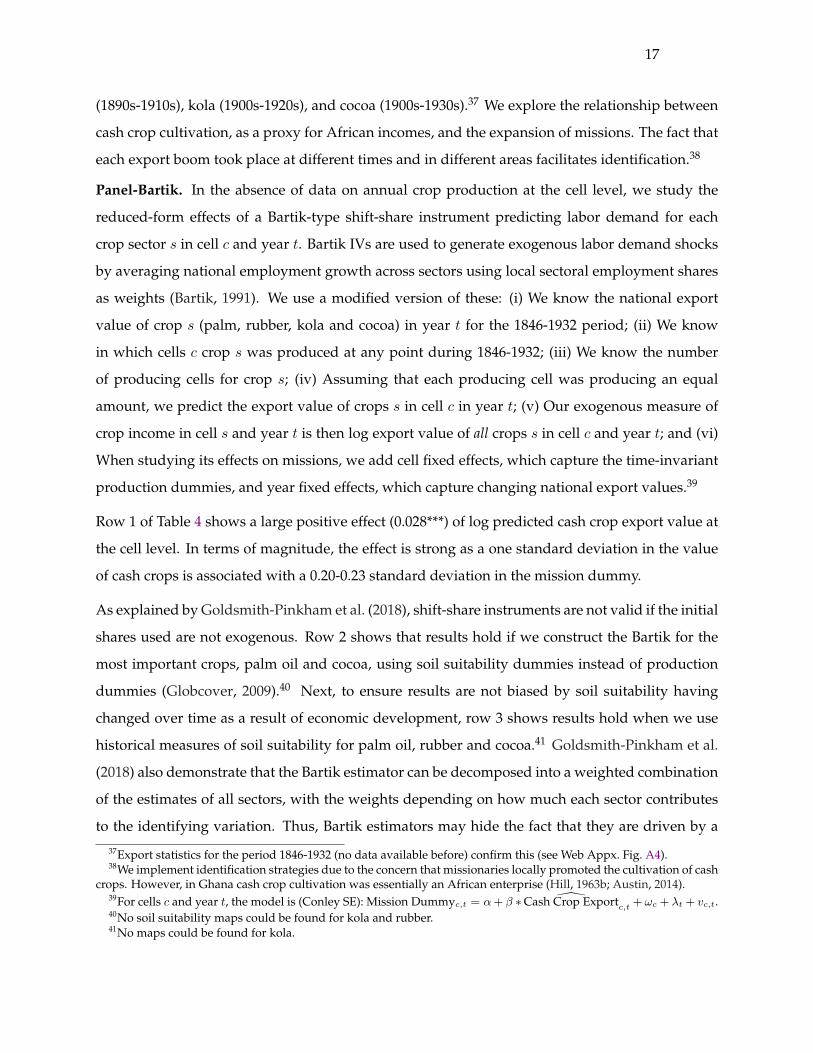
Panel-Bartik. In the absence of data on annual crop production at the cell level, we study the

reduced-form effects of a Bartik-type shift-share instrument predicting labor demand for each

crop sector s in cell c and year t. Bartik IVs are used to generate exogenous labor demand shocks

by averaging national employment growth across sectors using local sectoral employment shares

as weights (Bartik, 1991). We use a modified version of these: (i) We know the national export

value of crop s (palm, rubber, kola and cocoa) in year t for the 1846-1932 period; (ii) We know

in which cells c crop s was produced at any point during 1846-1932; (iii) We know the number

of producing cells for crop s; (iv) Assuming that each producing cell was producing an equal

amount, we predict the export value of crops s in cell c in year t; (v) Our exogenous measure of

crop income in cell s and year t is then log export value of all crops s in cell c and year t; and (vi)

When studying its effects on missions, we add cell fixed effects, which capture the time-invariant

production dummies, and year fixed effects, which capture changing national export values.39

Row 1 of Table 4 shows a large positive effect (0.028***) of log predicted cash crop export value at

the cell level. In terms of magnitude, the effect is strong as a one standard deviation in the value

of cash crops is associated with a 0.20-0.23 standard deviation in the mission dummy.

As explained by Goldsmith-Pinkham et al. (2018), shift-share instruments are not valid if the initial

shares used are not exogenous. Row 2 shows that results hold if we construct the Bartik for the

most important crops, palm oil and cocoa, using soil suitability dummies instead of production

dummies (Globcover, 2009).40 Next, to ensure results are not biased by soil suitability having

changed over time as a result of economic development, row 3 shows results hold when we use

historical measures of soil suitability for palm oil, rubber and cocoa.41 Goldsmith-Pinkham et al.

(2018) also demonstrate that the Bartik estimator can be decomposed into a weighted combination

of the estimates of all sectors, with the weights depending on how much each sector contributes

to the identifying variation. Thus, Bartik estimators may hide the fact that they are driven by a

37Export statistics for the period 1846-1932 (no data available before) confirm this (see Web Appx. Fig. A4).38We implement identification strategies due to the concern that missionaries locally promoted the cultivation of cash

crops. However, in Ghana cash crop cultivation was essentially an African enterprise (Hill, 1963b; Austin, 2014).39For cells c and year t, the model is (Conley SE): Mission Dummyc,t = α+ β ∗ Cash Crop Export

c,t+ ωc + λt + vc,t.

40No soil suitability maps could be found for kola and rubber.41No maps could be found for kola.

18

few sectors only, and the specific exogeneity of their shares must be discussed. In our case, we

rely on four crops – rather than say hundreds of industries – and rows 4-7 show results hold for

each crop one by one. Furthermore, we build another Bartik for cocoa for which we have detailed

geospatialized data on soil suitability. For each cell, we know the respective shares of moderately,

highly and very highly suitable soils, as well as the relative average yields of these different types

of soils. As seen in row 8 the estimated effect is similar to the baseline.42

Moreover, no spurious effects are found when adding one lead of the Bartik (row 9). Instead, the

effect of cash crops in t on missions in t is captured by a lag of the Bartik (row 10). This suggests

missions followed cash crop incomes. Rows 11-13 show that results hold when adding ethnic

group or district fixed effects interacted with year fixed effects or cell-specific linear trends.

Finally, the same Bartik analysis shows additional effects on the number of missions or the opening

of main stations once we control for whether the cell had a mission (see Web Appx. Table A7). The

same Web Appendix table also confirms that cash crop incomes have stronger effects on Mainline

Protestant missions than on Catholic missions or other Protestant missions. This is another piece

of evidence that economic considerations strongly mattered for missionary expansion.

Summary. A one standard deviation in malaria, railroads and cash crops is associated with a

0.08-0.18, 0.14-0.15 and 0.20-0.23 standard deviation increase in the mission dummy, respectively.

However, there is a possibility that our estimates for malaria are not causal. Nonetheless, crudely

adding these numbers, we obtain 0.42-0.56 (0.34-0.38 excl. malaria). Overall, the variables possibly

explain a significant share of missionary expansion over time. The analysis also does not account

for the effects of other locational factors or the general equilibrium effects of the three variables.

3.4. Dynamics of Missionary Expansion

This section highlights the dynamics of missionary expansion by documenting the changing

locational characteristics in the stock of missions over time. We construct a measure that

summarizes how “attractive” a location was to missionaries. More precisely, we regress the

mission dummy in 1932, Mc,1932, on all the possible determinants of mission placement Xc of

Table 1. We then obtain the predicted probability Mc,1932 = XcB, or locational score. We distinguish

between four groups of cells in 1840-1932:43 (i) cells with a mission in both t − 1 and t (“remains

42Very highly suitable soils include class 1 and class 2 ochrosols and produce about 2,000 pounds of dry cocoa peracre. Highly suitable soils include class 3 ochrosols and produce 1,338 pounds per acre. Suitable soils include othertypes of cocoa soils and produce 223 pounds per acre. See Web Data Appx. for details on the sources used.

43We use 1840 because it is the first year with 10 missions.

19

1”); (ii) cells with no missions in t − 1 but a mission opening in t (“becomes 1”); (iii) cells with a

mission in t − 1 that exits in t (“becomes 0”); and (iv) cells with no missions in both t − 1 and t

(“remains 0”). Figure 7(a) plots a quadratic fit of the average score for those four groups.

The pattern suggests that the best locations received missions first, and that marginally less good

locations were increasingly added to the existing stock of mission locations. Indeed, cells with

surviving missions (“remains 1”) rank consistently higher than cells that gain or lose missions

(“becomes 1” or “becomes 0”) and their scores significantly exceed those of the “remains 0” group.

Scores of all the four groups decrease over time. Scores of the “becomes 1” group decrease, because

less and less attractive mission locations are added over time. Scores of the “remains 0” group

decrease, because switchers are among the best locations of the cells with no missions.44

Results hold if (not shown): (i) We use the period 1751-1840 to estimate the coefficient of each

factor and study predicted scores post 1840; (ii) The urban share in 1931 is the predicted variable.

3.5. Replication of the Results for sub-Saharan Africa

We replicate the analysis of the determinants of missionary expansion for sub-Saharan Africa.

Obviously, unlike for Ghana, we have to rely on limited and possibly mismeasured data.

Descriptive Analysis. In Table 6, for 203,574 cells in 43 countries, we regress a dummy if there is a

mission according to the maps of Beach (1903), supposedly representing the year 1900 (col. (1)), or

Roome (1925), supposedly representing the year 1924 (col. (2)), on various locational factors and

country fixed effects. The regression is the same as for Ghana. Calculating Conley standard errors

is too computationally intensive for that many cells. We therefore cluster standard errors at the

district level (as of 2000). With 3,284 districts, we get about 62 cells per district.45 From the year of

foundation reported for 83% of Protestant missions in Beach (1903), we construct a quasi-panel.46

We then study in col. (3)-(5) how the correlations vary across three periods defined around four

turning points: 1792 (first year with a mission), 1850 (date when anti-slavery efforts intensified),

1881 (start of the Scramble for Africa), and 1900 (last year of mission data in Beach (1903)).

Missionaries appear to have chosen locations with healthier environments (malaria, tsetse).

Especially before 1850, missionaries seem to have avoided large pre-colonial cities, ethnic

44When regressing the scores of the “remains 1”, “becomes 1”, “becomes 0”, and “remains 0” groups on the year, wefind a significant negative effect: -0.003*** (R2 = 0.90), -0.005*** (0.46), -0.006*** (0.44), and -0.001*** (0.89), respectively.The high R2 values imply that the best-ness of a location is predicted by the year it gained or lost a mission.

45The main results (Table 5, Table 6 and panel B of Table 8) hold when using larger grid cells to cluster standarderrors, for example 10x10 mega-cells (N = 94 cells per mega-cell) or even 15x15 mega-cells (N = 199 cells) (not shown).

46To our knowledge, no one has ever used the panel aspect of this data. Panel data does not exist for Roome (1925).

20

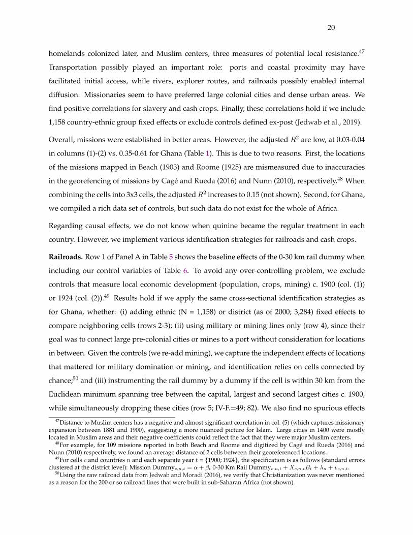
homelands colonized later, and Muslim centers, three measures of potential local resistance.47

Transportation possibly played an important role: ports and coastal proximity may have

facilitated initial access, while rivers, explorer routes, and railroads possibly enabled internal

diffusion. Missionaries seem to have preferred large colonial cities and dense urban areas. We

find positive correlations for slavery and cash crops. Finally, these correlations hold if we include

1,158 country-ethnic group fixed effects or exclude controls defined ex-post (Jedwab et al., 2019).

Overall, missions were established in better areas. However, the adjusted R2 are low, at 0.03-0.04

in columns (1)-(2) vs. 0.35-0.61 for Ghana (Table 1). This is due to two reasons. First, the locations

of the missions mapped in Beach (1903) and Roome (1925) are mismeasured due to inaccuracies

in the georefencing of missions by Cage and Rueda (2016) and Nunn (2010), respectively.48 When

combining the cells into 3x3 cells, the adjustedR2 increases to 0.15 (not shown). Second, for Ghana,

we compiled a rich data set of controls, but such data do not exist for the whole of Africa.

Regarding causal effects, we do not know when quinine became the regular treatment in each

country. However, we implement various identification strategies for railroads and cash crops.

Railroads. Row 1 of Panel A in Table 5 shows the baseline effects of the 0-30 km rail dummy when

including our control variables of Table 6. To avoid any over-controlling problem, we exclude

controls that measure local economic development (population, crops, mining) c. 1900 (col. (1))

or 1924 (col. (2)).49 Results hold if we apply the same cross-sectional identification strategies as

for Ghana, whether: (i) adding ethnic (N = 1,158) or district (as of 2000; 3,284) fixed effects to

compare neighboring cells (rows 2-3); (ii) using military or mining lines only (row 4), since their

goal was to connect large pre-colonial cities or mines to a port without consideration for locations

in between. Given the controls (we re-add mining), we capture the independent effects of locations

that mattered for military domination or mining, and identification relies on cells connected by

chance;50 and (iii) instrumenting the rail dummy by a dummy if the cell is within 30 km from the

Euclidean minimum spanning tree between the capital, largest and second largest cities c. 1900,

while simultaneously dropping these cities (row 5; IV-F.=49; 82). We also find no spurious effects

47Distance to Muslim centers has a negative and almost significant correlation in col. (5) (which captures missionaryexpansion between 1881 and 1900), suggesting a more nuanced picture for Islam. Large cities in 1400 were mostlylocated in Muslim areas and their negative coefficients could reflect the fact that they were major Muslim centers.

48For example, for 109 missions reported in both Beach and Roome and digitized by Cage and Rueda (2016) andNunn (2010) respectively, we found an average distance of 2 cells between their georeferenced locations.

49For cells c and countries n and each separate year t = {1900; 1924}, the specification is as follows (standard errorsclustered at the district level): Mission Dummyc,n,t = α+ βt 0-30 Km Rail Dummyc,n,t +Xc,n,tBt + λn + vc,n,t.

50Using the raw railroad data from Jedwab and Moradi (2016), we verify that Christianization was never mentionedas a reason for the 200 or so railroad lines that were built in sub-Saharan Africa (not shown).

21

when using placebo lines planned c. 1916-1922 but never built (row 6).

For the panel analysis of the effects of railroads, we restrict the sample to the 1885-1900 period.

Until 1885, only South Africa had railways and rail construction in Africa only expanded from

the late 1880s on. Unlike for Ghana, we only know the opening year of the railroad, not the

announcement year. In addition, for Africa the exact foundation year of each mission and the year

in which each railroad line was completed are both likely to be mismeasured. We therefore use 5

year panel data.51 Lastly, to reduce the number of observations, we restrict the sample to 103,866

cells in 15 countries with railroads opened at any point during 1885-1900, thus obtaining 103,866

x 4 = 415,464 observations.52 Panel B shows the baseline effect of row 7 is positive and significant.

Row 8 shows there is no effect when adding one lead of the rail dummy. However, row 9 indicates

that the contemporaneous effect of railroads in t on missions in t is not captured by the lag of the

rail dummy in t − 5. Next, Rows 10-11 show that point estimates remain similar when adding

ethnic group or district fixed interacted with year effects, to compare connected and unconnected

neighboring cells over time (effect not significant at 10% with district-year fixed effects). Finally,

including 103,866 cell-specific linear trends is unfortunately too computationally intensive.53

Overall, cross-sectional and panel estimates are similar, and a one standard deviation in the rail

dummy is associated with a 0.01-0.09 standard deviation in the mission dummy. The magnitude

of the effects is smaller than for Ghana (0.14-0.15). However, mission and railroad openings are

mismeasured for the whole of Africa making the comparison with the Ghana results less relevant.

Lastly, using the same cross-sectional or panel identification strategies, we find stronger effects

for Mainline Protestants than for Catholics or other Protestants (Web Appx. Tables A8-A9). Thus,

economic considerations also mattered more for Protestants when studying the determinants of

mission expansion for the whole continent.

Cash Crops. We implement the same panel-Bartik strategy as for Ghana.54 However, we only

have panel data on missions before 1900. In addition, for the seven crops studied for Africa (cocoa,

51The same reason also prevents us from performing an event study analysis.52For cells c, countries n, and years t, the model is (standard errors clustered at the district level): Mission

Dummyc,n,t = α + β 30 Km Rail Dummyc,n,t + ωc + λt + κn,t + vc,t. The 15 countries include 3 Central African,5 East African, 3 Southern African and 4 West African countries, respectively.

53Results generally hold if we add linear trends for 0.75x0.75, 0.60x0.60, 0.50x0.50, 0.40x0.40, 0.30x0.30 and 0.25x0.25degree mega-cells (not shown, but available upon request). The corresponding number of mega-cells increases from2,110 to 17,209 for railroads and from 1,523 to 11,817 for cash crops (see the next analysis).

54There is a concern that missionaries locally promoted crop cultivation in other countries than Ghana. However, inmost of colonial Africa, cash crop cultivation was driven by African initiative (Austin, 2014) - not mission societies.

22

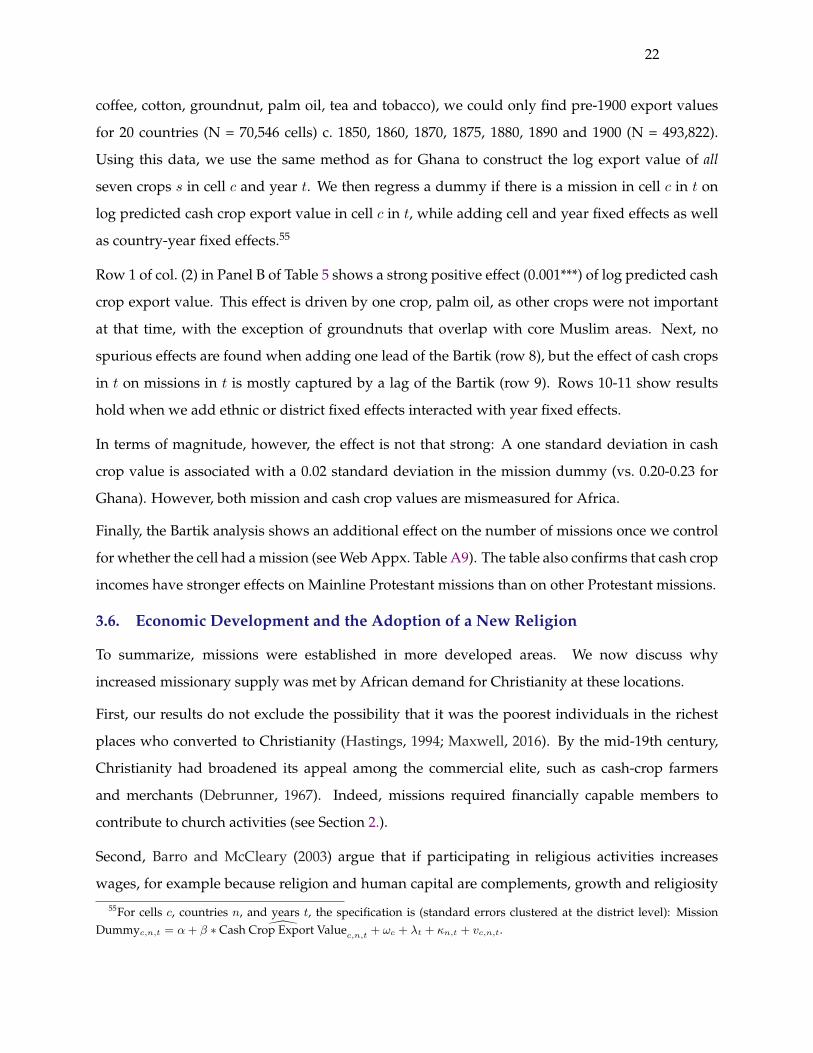
coffee, cotton, groundnut, palm oil, tea and tobacco), we could only find pre-1900 export values

for 20 countries (N = 70,546 cells) c. 1850, 1860, 1870, 1875, 1880, 1890 and 1900 (N = 493,822).

Using this data, we use the same method as for Ghana to construct the log export value of all

seven crops s in cell c and year t. We then regress a dummy if there is a mission in cell c in t on

log predicted cash crop export value in cell c in t, while adding cell and year fixed effects as well

as country-year fixed effects.55

Row 1 of col. (2) in Panel B of Table 5 shows a strong positive effect (0.001***) of log predicted cash

crop export value. This effect is driven by one crop, palm oil, as other crops were not important

at that time, with the exception of groundnuts that overlap with core Muslim areas. Next, no

spurious effects are found when adding one lead of the Bartik (row 8), but the effect of cash crops

in t on missions in t is mostly captured by a lag of the Bartik (row 9). Rows 10-11 show results

hold when we add ethnic or district fixed effects interacted with year fixed effects.

In terms of magnitude, however, the effect is not that strong: A one standard deviation in cash

crop value is associated with a 0.02 standard deviation in the mission dummy (vs. 0.20-0.23 for

Ghana). However, both mission and cash crop values are mismeasured for Africa.

Finally, the Bartik analysis shows an additional effect on the number of missions once we control

for whether the cell had a mission (see Web Appx. Table A9). The table also confirms that cash crop

incomes have stronger effects on Mainline Protestant missions than on other Protestant missions.

3.6. Economic Development and the Adoption of a New Religion

To summarize, missions were established in more developed areas. We now discuss why

increased missionary supply was met by African demand for Christianity at these locations.

First, our results do not exclude the possibility that it was the poorest individuals in the richest

places who converted to Christianity (Hastings, 1994; Maxwell, 2016). By the mid-19th century,

Christianity had broadened its appeal among the commercial elite, such as cash-crop farmers

and merchants (Debrunner, 1967). Indeed, missions required financially capable members to

contribute to church activities (see Section 2.).

Second, Barro and McCleary (2003) argue that if participating in religious activities increases

wages, for example because religion and human capital are complements, growth and religiosity

55For cells c, countries n, and years t, the specification is (standard errors clustered at the district level): MissionDummyc,n,t = α+ β ∗ Cash Crop Export Value

c,n,t+ ωc + λt + κn,t + vc,n,t.

23

go hand in hand. Missions supplied the bulk of formal education (Frankema, 2012), which

commanded a wage premium and facilitated occupational mobility (Ekechi, 1971; Frankema and

Van Waijenburg, 2019; Meier zu Selhausen et al., 2018). However, the complementarity between

Christianity and schooling weakened over time. In Ghana, since the 1870s missions increasingly

opened without government approved schools. In 1932, only one out of six missions had a school

(Figure 3). After World War II states expanded the supply of state schools and missions lost their

monopoly on schooling. Hence, schooling cannot fully account for the appeal of Christianity.

Third, Christianity disrupted the monopoly, and spread at the expense of, African traditional

religions. It has been argued that such religions constrained individual ownership and restricted

the pursuit of self-interest (Pauw, 1996; Alolo, 2007). Christianity, in particular the Protestant

denominations, are more capitalist in nature. There are also spiritual needs in a world where

established systems of meaning became increasingly disrupted by changing social and economic

circumstances, including new technologies (e.g., railroads and steamships). Africans sought a

measure of conceptual control over these forces by turning to the new ideas offered by Christianity

(Maxwell, 2016). Thus, Christianity may have been for converts a more this-worldly religion.

4. Implications for the Study of Long-Run Economic Development

Our results have several implications for the study of the long-run effects of colonial missions.

Most studies retrieve mission location data from a source different from ours: Historical mission

atlases. Using Ghana as an example, we first show that atlases select the most important missions

(e.g. early, main or European residence stations). Second, we will examine the long-term economic

and non-economic effects of missions when relying on atlas missions or census missions and the

standard controls used in the literature or our controls, and compare different types of missions.

4.1. Mission Atlases and Non-Classical Measurement Error in Missionary Activity

In the literature, two mission atlases feature prominently: Beach (1903) and Roome (1925).56

Yet, we find that atlases significantly underreport missions. For Ghana, atlases show far fewer

missions than census returns: 26 vs. 304 (91% are missing) in 1900 (Beach, 1903) and 23 vs. 1,213

(98%) in 1924 (Roome, 1925) (see Fig. 2(a)-2(b)). For Africa, the extent of misreporting is of similar

scale: Beach (1903) and Roome (1925) omitted 93% and 98% of missions (see Fig. 1(b)).57 If

56Based on Web Appx. Table A1, about 30 studies rely on either Beach (1903) or Roome (1925).57The extent of omissions is relatively similar across movements and denominations: Beach (1903) misses 89% of

Methodist missions and 92% of Presbyterian missions whereas Roome (1925) misses 97% of Protestant missions and

24

measurement error is classical, estimates of the contemporary effect of missions will be downward

biased. However, this is far from certain. Fahs (1925) pointed out that atlases overwhelmingly plot

residence stations of European missionaries. In this case, measurement error is non-classical.58

We can investigate the measurement error thanks to our unique data on census missions and their

characteristics. Examining the geographic distribution of missions in Ghana (see Fig. 2(a) and 2(b))

reveals two stylized facts. First, atlases miss most hinterland missions. Second, Roome (1925) does

not capture the exponential growth of missions between 1900 and 1924. We study this further by

calculating the coefficients of correlation between a dummy equal to one if there is an atlas mission

(1900, 1924) and a dummy equal to one if there is a census mission in a cell for each year (1840-

1932). Figure 7(b) shows high correlations for earlier years (0.8 for Beach (1903) and 0.4 for Roome

(1925)).59 Atlases thus best represent missions circa 1850 (that survived) instead of 1900, or 1924.

Atlas missions also differ qualitatively. In Table 7 we regress a dummy equal to one if there is

an atlas mission on cell-level mission characteristics derived from our data for the years 1900

and 1924. The correlations show that atlases capture not only early missions (col. (2) and (7)),

but also main stations as well as missions with schools (col. (3) and (8)) and the residences of

European missionaries (col. (4) and (9). Some characteristics are then correlated with each other

(col. (5) and (10)).60 The R2 is then 0.64-0.45 (0.79-0.55 with 2x2 cells). Overall, atlases selected

“better” missions. But, do atlases at least reliably select the “best” missions that received major

investments? The answer is no. If we define the “best” missions as the ones that were main

stations, where Europeans resided and which had a school, atlases still miss 68-83% of them.

4.2. Non-Classical Measurement Error and Long-Term Economic Effects

We now study the long-term economic effects of missions, depending on whether we rely on

census missions or atlas missions. We run a regression correlating a dummy equal to one if the

location had a mission (Mc,g) in 1900 or 1924 and economic development today (Dc,g,today):

Dc,g,today = a′′′ + ρMc,g +Xc,gζ + κ′g + wc (1)

99% of Catholic missions. Other atlases compare as follows: 25 vs. 432 Protestant missions (i.e., 94% of missions aremissing) in 1908 (Bartholomew et al., 1911) and 6 vs. 49 Catholic missions (88%) in 1913 (Streit, 1913).

58Fahs (1925, p. 271) wrote that “[...] mapping the Christian advance which puts a red underline under someplace-name to indicate the residence of a British or Continental or American missionary, but does not indicate wherean Azariah or a Kagawa serves his people, fails to give needful perspective.” Mission atlases thus ignore the verysignificant contribution of African missionaries to Christian expansion (Meier zu Selhausen, 2019).

59When combining cells into 2x2 cells to account for possible inaccuracies in the geocoding of atlas missions, thecorrelation of earlier years is 0.9 for Beach (1903) and 0.7 for Roome (1925) (not shown).

60The variables still describe different mission characteristics. Correlation coefficients between the eight variablesaverage 0.45 (28 combinations), so much lower than 1.

25

Given the lack of data on incomes at the local level, we use log average night light intensity in

2010 – i.e., the total sum of night lights divided by area – as development indicator (Dc,g,today).

To avoid issues related to top-coding, we use the radiance calibrated version of this data (NOAA,

2012), which records levels of luminosity beyond the normal digital number upper bound of 63.61

For both Ghana and Africa, we examine how ρ varies if we include: (i) No controls Xc,g; (ii) The

“standard” controls commonly used in the literature on Africa (Std). In particular, we merge the

lists of controls from Nunn (2010, 2014) and Cage and Rueda (2016). Small variations over this set

of controls have been used, for example, by Fenske (2015), Okoye (2021), Henn et al. (2019) and

Cage and Rueda (2020).62; (iii) Our full set of possible determinants from Table 1 (Ghana) or Table 6

(Africa) (Ours); and (iv) Our full set of controls as well as controls for the type of mission. The latter

include (only available for Ghana; from Table 7) whether the mission was created in 1751-1850 or

1851-75, is a main station in t, has a school in t, a European missionary lived there in 1846-90, and

a European missionary frequently visited the mission in 1846-90. When controlling for the type,

the effect is estimated for average missions, which minimizes external validity concerns.

Table 8 presents the results. For Ghana, using the census mission dummy (row 1 of Panel A), we

find large unconditional effects of 1.05***-0.84*** (col. (1) and (6)). Adding the standard controls

reduces the estimated effect to 0.78***-0.73*** (col. (2) and (7)). An early colonial mission thus

(relatively) increases night lights by 117-107%, or 0.35-0.49 if expressed in terms of standard

deviations.63 Next, with the imperfectly measured Africa controls (from Table 6), the effect is

further reduced by almost 50%, to 0.41***-0.38*** (col. (3) and (8)). If we use our extended set

of Ghana controls, the effect is further divided by 2 or even 3, to 0.12-0.19*** (col. (4) and (9)).64

Lastly, also controlling for the type of missions, the effect decreases to 0.01-0.17*** (col. (5) and

61Nightlights have become a standard measure in the stream of literature that studies development at the local levelin Africa (Michalopoulos and Papaioannou, 2013, 2014; Alesina et al., 2016; Michalopoulos and Papaioannou, 2018).

62Nunn (Table 1, 2010, 2014) uses: (i) European explorer routes before colonization; (ii) 19th century railroads; (iii) soilquality; (iv) access to a water source; and (v) slave exports. For Ghana: (i) There were no explorers before officialcolonization (there is thus no variation across cells); (ii) There was no railroad before 1901 (ditto); (iii) We controlfor soil fertility; (iv) We add a dummy if the cell is within 10 km from a navigable river (there were no lakes then);and (v) We control for slave export intensity. Cage and Rueda (Table 1, 2016, 2020) add: (vi) rainfall; (vii) distance to thecoast; (viii) malaria ecology; (ix) initial population density; and (x) dummies if large cities in 1400 or 1800. For Ghana: (vi) Wecontrol for rainfall; (vii) We control for distance to the coast; (viii) We control for malaria; (ix) We control for populationdensity in 1800; and (x) We add a dummy if there was a large city in 1800 (none in 1400).

63117-107 comes from applying the formula 100 (exp(b - V(b)/2) - 1) (Halvorsen and Palmquist, 1980; Kennedy, 1981).64One concern is that some of our controls are defined ex-post. If we exclude or adjust the timing of these controls,

the estimated effects (c. 0.25***) are still two thirds lower than with the standard controls (not shown). We use roadsc. 1900 and c. 1924 (instead of 1930). For 1924, we use railroads c. 1924 (instead of 1932). We exclude urban and ruralpopulations in 1931 and the crop variables. However, our palm oil (measured in 1900-36), rubber (1900-36) and kola(1932) controls reflect conditions before 1924 (or even 1900) since these cash crops boomed early (section 3.3.). Cocoa isa perennial crop, and harvest begins after 5 years. Cocoa production c. 1927 reflects cocoa cultivation in 1922 or before.

26

(9)). One standard deviation in the mission dummy is then associated with a 0.00-0.12 increase

in the standard deviation in log night lights.65 Therefore, we find that the average (census-based)

missions had possibly no or weak effects on contemporary development in Ghana.66

However, atlas missions, because they capture important missions, could still have strong long-

term economic effects, especially if we do not control for their potentially endogenous placement

and type. In row 2 of Panel A, we use the same model as in row 1 but, instead of the census

mission dummy, we include an atlas mission dummy and a non-atlas mission dummy (defined as

census mission dummy - atlas mission dummy). Without controls, we obtain twice larger point

estimates for atlas missions. The effect of atlas missions is still much larger, by 0.74*** (not shown),

if we add the standard controls (col. (2) and (7)). Once we add our controls, including the type of

missions (col. (5) and (10)), we again find nil or small effects for non-atlas mission (0.01-0.17***).

Although atlas missions have a stronger effect, the difference with respect to non-atlas missions

is barely significant (0.43*; col. (5)) or insignificant (0.15; col. (10)).67 More generally, using our

full controls rather than the standard controls decreases the effects of atlas missions for Ghana by

(1-0.44/1.39)*100 = 68% for Beach and (1-0.33/1.43)*100 = 77% for Roome.68

In row 3, Panel A of Table 8, we study the effects for Ghana if we only include the atlas mission

dummy, in order to mimic the regressions we are running for Africa next. When doing so,

the effect of atlas missions is slightly lower than when controlling for the non-atlas missions.

However, the same patterns as before emerge. Using our full controls rather than the standard

controls decreases the effects of atlas missions for Ghana by 65-85%.

Finally, in Panel B, we examine for 43 African countries the effects of atlas missions on

contemporary night lights. The unconditional effect is 0.70*** (col. (1) and (6)). Adding the

standard controls reduces the effect to 0.60-0.59*** (col. (2) and (7)). Thus, a colonial mission

increases night lights by 82-80%, or 0.10-0.13 if expressed in terms of standard deviations. Adding

our Africa controls then lowers the effect to 0.37-0.40*** (we found 0.43-0.59*** for Ghana, see

row 3), or 0.07-0.08 if expressed in terms of standard deviations. If we also add two dummies for

65We do not over-control for the number of missions here. If we do, we obtain -0.26*** and 0.05 (not shown).66Note that we cannot distinguish whether the standard controls produce biased estimates because they do not

capture selection on unobservables (missions were established in places likely to be developed even in the absence of amission) or selection on beta (missions were established where the population was already receptive to missions ideas,and this pre-disposition could have contributed to long-run economic development).

67Without the ex-post controls, the atlas effect is three times lower than with the standard ones (not shown).68Ultimately, with our full controls, a census mission increases night lights by 1-18% whereas an atlas missions

increases night lights by 37-52%. Jedwab and Moradi (2016) find that a railroad built in Ghana before 1918 increasesnight lights by 365% (the coefficient is 1.64 but we use the standard formula 100 (exp(b - V(b)/2) - 1)).

27

whether a Beach mission already existed pre-1850 or in 1850-1881 – our only type control for Africa

–, the effect for the year 1900 decreases further to 0.28*** (not shown), which is about half the effect

with the standard controls. However, the Africa controls are not as precisely measured as those

for Ghana.69 We also just showed how using better controls reduces the effects of atlas missions

by 65-85% for Ghana. Were this the case for Africa, the standardized effect would only be 0.02.

4.3. Extensions

Measurement Error in the Controls. If the best missions are selected, the long-term effects

of missions will be over-estimated. The same is true if only mismeasured controls of mission

placement are available. For example, for the Africa regressions, we have no choice but to use

the Murdock (1967) map to obtain data on state centralization, slavery and polygamy. As such,

the reported estimates when using our full controls likely remain upward-biased. As we just

showed, the better measured Ghana controls, which do not rely on continental maps, reduce

the effects twice as much as the Africa controls. Now, if we drop the Murdock controls and

instead add ethnicity, country-ethnicity, province or district (as of 2000) fixed effects, the Africa

effects slightly decrease to about 0.30***-0.35*** (see Panel A of Web Appx. Table A10). However,

the mean province is large in Africa, with an area of 228,000 sq km vs. 197,000 on average for

U.S. states. The mean ethnic territory (141,000) and the mean district (84,000) are then 1.4 and 2.3

times smaller than the average U.S. state, which is still large. For Ghana, when using the standard

controls (see Panel B of Web Appx. Table A10), adding province, ethnicity or district fixed effects

only reduces the 1900-based effect from 0.78*** to 0.74***, 0.58*** and 0.51***, respectively, vs. 0.01

with our full controls. The 1924-based effect only decreases from 0.73*** to 0.68***, 0.60*** and

0.50***, respectively, vs. 0.17*** with our full controls. Thus, the standard controls do not capture

the fact that missionaries went to more developed areas within these spatial units.

Spillovers. Our main unit of analysis are grid cells of 0.1 x 0.1 degrees (12x12 km). The minimal

distance from the centroid of the cell to its edge is 6 km, or a one-hour walking distance. Due to the

lack of transportation technology, missions were likely to only influence local development during

the colonial era. However, spillovers remain a possibility. We use the same model as before but

also add the log of the minimal distance to a cell with a mission. When doing so, we find strong

69For example, we use the pre-colonial explorer routes digitized by Nunn and Wantchekon (2011). This is animperfect measure of pre-missionary era trade routes. For Ghana, this database returns 581 km of explorer routes(percentage of grids within 10 km of a route = 4.8%), whereas our sources indicate 6,526 km of trade routes (30.0%).For Madagascar, Nunn and Wantchekon (2011) do not record any explorer routes, whereas a different source suggeststhat all mission stations are clustered along explorer routes and the coast (see Web Appendix Figure A5).

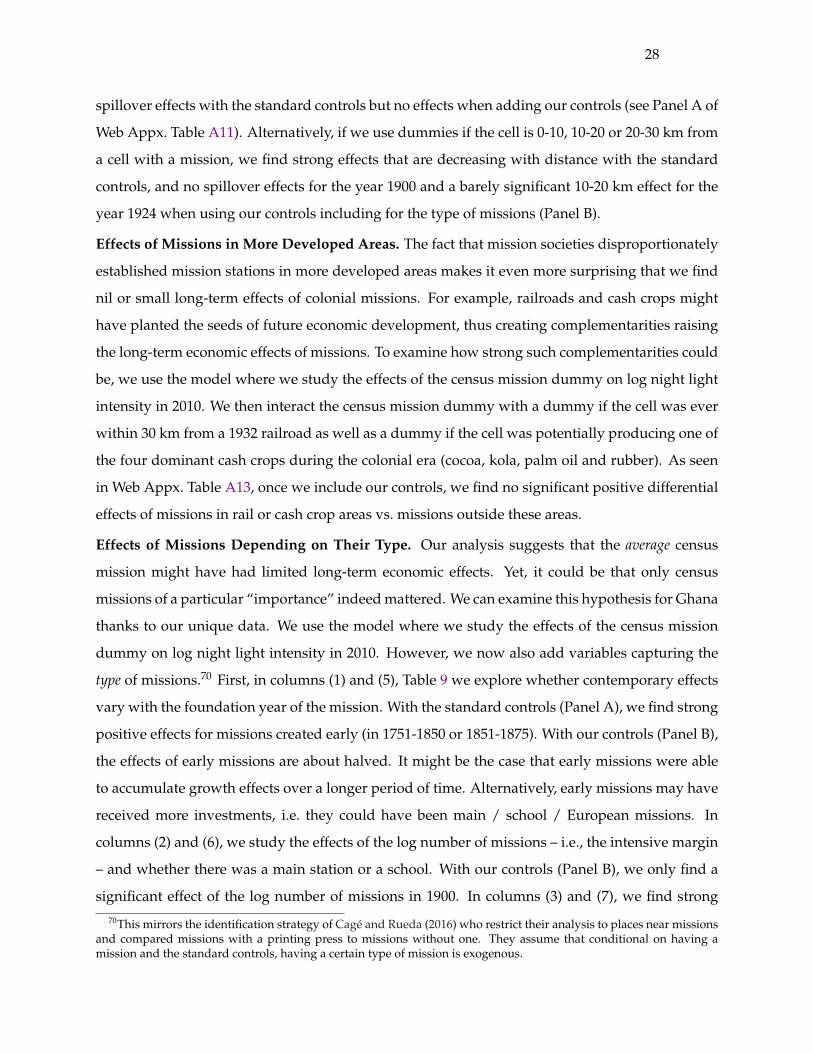
28

spillover effects with the standard controls but no effects when adding our controls (see Panel A of

Web Appx. Table A11). Alternatively, if we use dummies if the cell is 0-10, 10-20 or 20-30 km from

a cell with a mission, we find strong effects that are decreasing with distance with the standard

controls, and no spillover effects for the year 1900 and a barely significant 10-20 km effect for the

year 1924 when using our controls including for the type of missions (Panel B).

Effects of Missions in More Developed Areas. The fact that mission societies disproportionately

established mission stations in more developed areas makes it even more surprising that we find

nil or small long-term effects of colonial missions. For example, railroads and cash crops might

have planted the seeds of future economic development, thus creating complementarities raising

the long-term economic effects of missions. To examine how strong such complementarities could

be, we use the model where we study the effects of the census mission dummy on log night light

intensity in 2010. We then interact the census mission dummy with a dummy if the cell was ever

within 30 km from a 1932 railroad as well as a dummy if the cell was potentially producing one of

the four dominant cash crops during the colonial era (cocoa, kola, palm oil and rubber). As seen

in Web Appx. Table A13, once we include our controls, we find no significant positive differential

effects of missions in rail or cash crop areas vs. missions outside these areas.

Effects of Missions Depending on Their Type. Our analysis suggests that the average census

mission might have had limited long-term economic effects. Yet, it could be that only census

missions of a particular “importance” indeed mattered. We can examine this hypothesis for Ghana

thanks to our unique data. We use the model where we study the effects of the census mission

dummy on log night light intensity in 2010. However, we now also add variables capturing the

type of missions.70 First, in columns (1) and (5), Table 9 we explore whether contemporary effects

vary with the foundation year of the mission. With the standard controls (Panel A), we find strong

positive effects for missions created early (in 1751-1850 or 1851-1875). With our controls (Panel B),

the effects of early missions are about halved. It might be the case that early missions were able

to accumulate growth effects over a longer period of time. Alternatively, early missions may have

received more investments, i.e. they could have been main / school / European missions. In

columns (2) and (6), we study the effects of the log number of missions – i.e., the intensive margin

– and whether there was a main station or a school. With our controls (Panel B), we only find a

significant effect of the log number of missions in 1900. In columns (3) and (7), we find strong70This mirrors the identification strategy of Cage and Rueda (2016) who restrict their analysis to places near missions

and compared missions with a printing press to missions without one. They assume that conditional on having amission and the standard controls, having a certain type of mission is exogenous.

29

effects of more European missions. The effects are about halved with our controls. Finally, if we

add all characteristics and our controls (Panel B), the only effects that remain significant are for

missions ‘created 1851-1875’ and the log number of missions in 1900. Hence, controlling for early

creation and density, we find no effects for main / school / European missions, which is surprising

since these are characteristics that one might have expected to matter.71

Other Strategies. We find similar non-results on long-term economic development if we employ

other strategies. In Panel A of Web Appx. Table A16, we compare cells with Protestant missions,

Catholic missions, and no missions (Nunn, 2014; Cage and Rueda, 2020). With the standard

controls, we find higher point estimates for Protestant missions. With our controls, point estimates

are much lower, and their difference is reversed. We also compare cells where missions survived

with cells where missions were abandoned as in Valencia Caicedo (2019a). For the year 1924, we

find strong effects with the standard controls and no effects with our controls (Panel B).

Example from the Literature. Nunn (2014)’s seminal study uses the atlas missions from Roome

(1925) and survey data from the 3rd round of the Afrobarometer Surveys (2005-06) to study the

effects of colonial-era missions on education for individuals aged 18 or older. Col. (1) of Nunn’s

Table 1 regresses the respondent’s educational attainment on the log number of atlas missions

per 1,000 km among the respondent’s ethnic group, adding country fixed effects, individual-level

controls (age, gender, urban) and ethnicity-level controls (see footnote 57). Col. (2) of Nunn’s Table

1 then uses the log number of atlas missions per 1,000 km within 25 km from the respondents’

village/residence as variable of interest (controls now defined at the cluster level).

Col. (1) of Panels A-B in our Web Appx. Table A12 reports Nunn’s main results for the first

specification (0.10**) and second specification (0.14***), respectively. In columns (2), we replicate

these Africa results, also using the respondent as the main unit of observation (standard errors

clustered at the ethnic group level). However, we use the 5th round of the Afrobaromater Surveys

(2011-13), which is closest to the year in which night lights are measured, includes 26 countries

instead of 17, and has almost twice as many observations (N = 38,087 respondents belonging

to 286 groups/5,776 clusters vs. 20,914 respondents belonging to 185 groups/2,693 clusters in

Nunn (2014). We obtain similar results (0.13***-0.13***). However, once we include our Africa

controls at the ethnicity or cluster level (col. (3)) and controls for whether the cell already had

Beach (1903) missions in the early years 1850, 1881 or 1900, an imperfect proxy for the “type” of

71The effects of early creation and density could be causal or reflect the fact that locations that received missions early,or had great demand for many missions, were special in ways not captured by our controls.

30

mission (col. (4)), the effects decrease by four times, and are not statistically significant for the

first specification. The standardized effects are only 0.02-0.03. If we then use Nunn’s cluster level

specification for Ghana (Panel C), we find no significant effects with our controls (col. (4)).72 If we

use our complete set of census missions in Ghana, we still find no effects (Panel D).

Other Outcomes. Since the literature has focused on the effects of colonial missions on proximate

determinants of economic growth, we now use the same framework to study the long-term effects

of the census missions on factors such as employment, education, health, and net fertility. The

data added in this analysis is retrieved from Ghana’s 2000 Population and Housing Census. When

studying child mortality, we rely on the geospatialized Demographic and Health Surveys (DHS)

(1993, 1998, 2003, 2008, 2014, 2016, and 2017). Details on the data can be found in Section 1.

Our analysis of night-lights in Ghana revealed that our controls (including the type of missions)

make the effect of missions disappear or reduce it by 4-6 times compared to when only the

standard controls are included. If we use instead the log of the cell’s urban population or the

urban share of the cell, our controls reduce the long-term effect of missions by 6-12 times relative

to the standard controls (rows 1-2 of Web Appx. Table A14).73 If we use log total population, our

controls make any effect of missions statistically insignificant (row 3).74

If we use the employment shares of industry and services (row 4), manufacturing and financial,

real estate and business services (FIRE) – arguably the “best” industrial and service sectors (Gollin

et al., 2016) – (row 5), or skilled occupations75 (row 6), we find that our controls reduce the long-

term effects of missions on these by 5-9, 5-8 and 4 times, respectively. In terms of standardized

effects, we find 0.00-0.12 for night lights, 0.02-0.03 for urbanization and 0.05-0.09 for employment.

Row 7 of Web Appx. Table A14 uses as the dependent variable the population share of Protestants

and Catholics in 2000. Our controls barely change the long-run effect of missions on Christianity.

The standardized effects are 0.08-0.15, higher than for economic outcomes.

If we use the number of years of education (row 8) or the primary completion rate (row 9) for

individuals aged 18 or more in 2000, our controls reduce the effects by about 3 times relative to the

standard controls. If we use height- or weight-for-age z-scores for children below 5 in 1993-2017

72The effect in column (1) is only significant at the 10% level due to the low number of observations. We do not usethe first specification for Ghana because only 17 Murdock ethnicities are present in the Afrobaromater data.

73Consistent with the 2000 census, we define as urban any locality above 5,000.74The effects on log night light intensity are then mostly unchanged when controlling for log urban population (not

shown but available upon request), implying that log night light intensity mostly captures per capita incomes.75These include managers, professionals, technicians, and clerks.

31

(source: DHS), our controls reduce the effects by 1.3-2.0 times relative to the standard controls

(rows 10-11). Thus, our controls reduce the effects by more than they do for Christianity, and less

than they do for economic outcomes. Also, the standardized effects are 0.10-0.17 for education

and 0.04-0.09 for health, similar or higher than for economic outcomes.76

Our controls reduce the effects of missions on completed fertility (row 12) and net completed

fertility (row 13) – for 35-49 aged women in 2000 – by 2-4 times and 2.5-5 times relative to the

standard controls, respectively. Completed (child) mortality then does not vary with missions

(row 14). In terms of standardized effects, with our full controls, we find -0.03/-0.08 for net fertility,

which is similar in size to economic outcomes.

Overall, we find stronger, but still weak, effects on education, health, and fertility, implying that

missions might have affected development outcomes without spurring economic development.77

Way Forward and External Validity. Our paper proposes a number of potentially important

predictors for colonial missions. In principle, those predictors can be used in matching procedures

or as instrumental variables for the placement of missions. However, our set of determinants is

not exhaustive. Hence, the exogeneity assumption may be violated. In addition, our results are

specific to the African context. In other contexts such as in Latin America, missionaries activities

and colonial infrastructure and economic investments were often jointly determined by colonial

governments and the Catholic Church (Valencia Caicedo, 2019a,b). Missions were then more likely

“proxies” for colonization in general, making it more difficult to isolate the effects of missions

themselves.78

5. Conclusion

In this paper, we studied Christian missions, a major human capital promoting institution that

emerged during colonial times. We argued that in order to estimate colonial missions’ long-

term economic impact, one needs a better understanding of the dynamics and economics of

76In Ghana, missions did not invest into health care. Elsewhere, missions were often the only health care providersduring the colonial era (Cage and Rueda, 2020). Still, few missions offered health services. Of all missions only 2% and4% of Catholic (in 1910) and Protestant (in 1923) missions respectively operated a hospital (Streit, 1913; Beach and Fahs,1925). Such investments were costly to missions because they were free of charge for most patients (Doyle et al., 2020).

77As shown in Web Appx. Table A15, we do not find any significant positive effects of main / school / Europeanmissions on educational outcomes today. We also find nil or contradictory effects for health outcomes. Finally, whethermain stations or mission schools significantly reduce net fertility depends on whether we consider 1900 or 1924.

78In Ghana and other British colonies in Africa, the activities of the various mission societies and colonialinfrastructure and economic investments were not coordinated. In Belgian, French, Portuguese and Spanish colonies,coordination was also minimal, thus more similar to the Anglo-Saxon model of privatized missionary markets than tothe Spanish/Portuguese model of “bundled” colonization/missionization historically observed in Latin America.

32

missionary expansion. Focusing on Ghana and Africa, we described how missionaries privileged

healthier, more accessible, and richer places first. In particular, we showed how - with quinine -

malaria became less of an impediment, and how transport infrastructure and agricultural export

commodities attracted missions. The diffusion of Christianity, education and culture depends on

spatial patterns of economic development, even at low income levels. We then showed how non-

classical measurement error in mission atlases and omitted variable bias are concerns that could

lead to an overly optimistic account of the importance of missions for contemporary development.

ReferencesAcemoglu, Daron, Francisco A. Gallego, and James A. Robinson, “Institutions, Human Capital, and

Development,” Annual Review of Economics, 2014, 6 (1), 875–912.Agbeti, J. Kofi, West African Church History, Leiden: E.J. Brill, 1986.Ajayi, Jacob Festus Ade and Michael Crowder, History of West Africa, London: Longman, 1974.Alesina, Alberto, Sebastian Hohmann, Stelios Michalopoulos, and Elias Papaioannou, “Intergenerational

Mobility in Africa,” Working Paper 25534, National Bureau of Economic Research February 2019., Stelios Michalopoulos, and Elias Papaioannou, “Ethnic Inequality,” Journal of Political Economy, 2016, 124 (2),428–488.

Alolo, Namawu Alhassan, African Traditional Religion and Concepts of Development: A Background Paper 2007.Alsan, Marcella, “The Effect of the TseTse Fly on African Development,” American Economic Review, 2015, 105 (1),

382–410.Athey, Susan and Guido W. Imbens, “Design-based Analysis in Difference-In-Differences Settings with Staggered

Adoption,” NBER Working Papers 24963, National Bureau of Economic Research, Inc August 2018.Austin, Gareth, “African Rural Capitalism, Cocoa Farming and Economic Growth in Colonial Ghana,” in Toyin

Falola, ed., Ghana in Africa and the world: essays in honor of Adu Boahen, Trenton, NJ: Africa World Press, 2003,pp. 437–453., “Explaining and evaluating the cash crop revolution in the ”peasant” colonies of tropical Africa, ca. 1890-ca.1930: Beyond ”vent for surplus”,” in Emmanuel Akyeampong, Robert H. Bates, Nathan Nunn, and JamesRobinson, eds., Africa’s Development in Historical Perspective, New York: Cambridge University Press, 2014,pp. 295–320.

Bai, Ying and James Kai sing Kung, “Diffusing knowledge while spreading God’s message: Protestantism andeconomic prosperity in China, 1840-1920,” Journal of the European Economic Association, 2015, 13 (4), 669–698.

Barro, Robert J. and Rachel M. McCleary, “Religion and Economic Growth across Countries,” AmericanSociological Review, 2003, 68 (5), 760–781.and , “Which Countries Have State Religions?,” The Quarterly Journal of Economics, 2005, 120 (4), 1331–1370.and , “Protestants and Catholics and educational investment in Guatemala,” AEI Economics Working

Papers 928714, American Enterprise Institute May 2017.Bartholomew, J. G., James S. Dennis, Harlan P. Beach, and Charles H. Fahs, World Atlas of Christian Missions:

containing a directory of missionary societies, a classified summary of statistics, an index of mission stations, and mapsshowing the location of mission stations throughout the world, New York: Student Volunteer Movement for ForeignMissions, 1911.

Bartik, Timothy, Who Benefits from State and Local Economic Development Policies? 1991.Basel Mission, Report of the Basel Evangelical Mission on the Gold Coast, West-Africa, 1900, Basel: Evangelische

Missionsgesellschaft Basel, 1900.Beach, Harlan P., A Geography and Atlas of Protestant Missions: their environment, forces, distribution, methods,

problems, results and prospects at the opening of the twentieth century, Vol. 2, New York: Student VolunteerMovement for Foreign Missions, 1903.and Charles H. Fahs, World Missionary Atlas, New York: Institute of Social and Religious Research, 1925.

Becker, Sascha O. and Ludger Woessmann, “Was Weber Wrong? A Human Capital Theory of Protestant EconomicHistory,” The Quarterly Journal of Economics, 2009, 124 (2), 531–596.and , “Not the opium of the people: Income and secularization in a panel of Prussian counties,” American

Economic Review: Papers and Proceedings, 2013, 103 (3), 539–544.

33

, Markus Nagler, and Ludger Woessmann, “Education and religious participation: city-level evidence fromGermany’s secularization period 1890-1930,” Journal of Economic Growth, 2017, 22 (3), 273–311., , and , “Education and religious participation: city-level evidence from Germany’s secularization period1890–1930,” Journal of Economic Growth, September 2017, 22 (3), 273–311., Steven Pfaff, and Jared Rubin, “Causes and consequences of the Protestant Reformation,” Explorations inEconomic History, 2016, 62 (C), 1–25.

Bergeron, Augustin, “Religion and the Scope of Morality: Evidence from Exposure to Missions in the DRC,”Unpublished manuscript Harvard University, 2020.

Bisin, Alberto and Thierry Verdier, ““Beyond the Melting Pot”: Cultural Transmission, Marriage, and theEvolution of Ethnic and Religious Traits,” The Quarterly Journal of Economics, 2000, 115 (3), 955–988.

Bollinger, Christopher R., “Bounding mean regressions when a binary regressor is mismeasured,” Journal ofEconometrics, August 1996, 73 (2), 387–399.

Borusyak, Kirill and Xavier Jaravel, “Revisiting Event Study Designs, with an Application to the Estimation ofthe Marginal Propensity to Consumea,” Mimeo, 2016.

Cage, Julia and Valeria Rueda, “The Long-Term Effects of the Printing Press in Sub-Saharan Africa,” AmericanEconomic Journal: Applied Economics, 2016, 8 (3), 69–99.and , “Sex and the mission: The conflicting effects of early Christian missions on HIV in sub-Saharan

Africa,” Journal of Demographic Economics, 2020, 86 (3), 213–257.Caicedo, Felipe Valencia, “The Mission: Human Capital Transmission, Economic Persistence and Culture in

South America,” The Quarterly Journal of Economics, 2019, 134 (1), 507–556., “Missionaries in Latin America and Asia: A First Global Mass Education Wave,” in David Mitch and GabrieleCappelli, eds., Globalization and the Rise of Mass Education, London: Palgrave Macmillan, 2019, pp. 61–98.

Calvi, Rossella and Federico G. Mantovanelli, “Long-Term Effects of Access to Health Care: Medical Missions inColonial India,” Journal of Development Economics, 2018., , and Lauren Hoehn Velasco, “The Protestant Legacy: Missions and Human Capital in India,” Journal ofHuman Resources, 2021.

Cantoni, Davide, “Adopting a New Religion: the Case of Protestantism in 16th Century Germany,” The EconomicJournal, 2012, 122 (560), 502–531.

Castello-Climent, Amparo, Latika Chaudhary, and Abhiroop Mukhopadhyay, “Higher Education andProsperity: From Catholic Missionaries to Luminosity in India,” The Economic Journal, 2018, 128 (616), 3039–3075.

Chandler, Tertius, Four Thousand Years of Urban Growth: An Historical Census, Lewiston, NY: St. David’s UniversityPress, 1987.

Cleall, Esme, “Missionaries, Masculinities and War: The London Missionary Society in Southern Africa,c.1860–1899,” South African Historical Journal, 2009, 61 (2), 232–253.

Cogneau, Denis and Alexander Moradi, “Borders That Divide: Education and Religion in Ghana and Togo SinceColonial Times,” The Journal of Economic History, 2014, 74 (3), 694–729.

Conley, T. G., “GMM estimation with cross sectional dependence,” Journal of Econometrics, September 1999, 92 (1),1–45.

Curtin, Philip D., ““The White Man’s Grave”, Image and Reality, 1780-1850,” Journal of British Studies, 1961, 1 (1),94–110., The Image of Africa: British Ideas and Action, 1780-1850, Volume 2, Madison: University of Wisconsin Press, 1973.

Debrunner, Hans W., A History of Christianity in Ghana, Accra: Waterville Publishing House, 1967.Depetris-Chauvin, Emilio and David N. Weil, “Malaria and Early African Development: Evidence from the Sickle

Cell Trait,” The Economic Journal, 2018.Dickson, Kwamina B., A historical geography of Ghana, London: Cambridge University Press, 1969.Doyle, Shane, Felix Meier zu Selhausen, and Jacob Weisdorf, “The Blessings of Medicine? Patient Characteristics

and Health Outcomes in a Ugandan Mission Hospital, 1908–1970,” Social History of Medicine, 2020, 33 (3),946–980.

Ekechi, F. K., “Colonialism and Christianity in West Africa: The Igbo Case, 1900-1915,” The Journal of AfricanHistory, 1971, 12 (1), 103–115.

Engel, P. Alois, Die Missionsmethode der Missionare vom Hl. Geist auf dem afrikanischen Festland, Neuss: MissionshausKnechtsteden, 1931.

Fahs, Charles H., “On Making a Missionary Atlas,” International Review of Mission, 1925, 14 (2), 260–273.FAO, “GAEZ Global Agro-Ecological Zones (GAEZ v3.0),” 2012.Fenske, James, “African polygamy: Past and present,” Journal of Development Economics, 2015, 117, 58–73.Fischer, Friedrich Hermann, Der Missionsarzt Rudolf Fisch und die Anfange medizinischer Arbeit der Basler Mission an

der Goldkuste, Herzogenrath: Verlag Murken-Altrogge, 1991.Foster, Philip, Education and Social Change in Ghana, Chicago: University of Chicago Press, 1965.

34

Frankema, Ewout, “The Origins of Formal Education in sub-Saharan Africa: Was British Rule More Benign?,”European Review of Economic History, 2012, 16 (4), 335–355.and Marlous Van Waijenburg, “The Great Convergence. Skill Accumulation and Mass Education in Africa andAsia, 1870-2010,” CEPR Discussion Paper 14150, 2019.and Morten Jerven, “Writing history backwards or sideways: towards a consensus on African population,

1850–2010,” The Economic History Review, 2014, 67 (4), 907–931., Jeffrey G. Williamson, and Peter Woltjer, “An Economic Rationale for the West African Scramble? TheCommercial Transition and the Commodity Price Boom of 1835-1885,” The Journal of Economic History, 2018,78 (2), 231–267.

Gallego, Francisco A. and Robert D. Woodberry, “Christian Missionaries and Education in Former AfricanColonies: How Competition Mattered,” Journal of African Economies, 2010, 19 (3), 294–329.

Galor, Oded, “From Stagnation to Growth: Unified Growth Theory,” in Philippe Aghion and Steven Durlauf,eds., Handbook of Economic Growth, Elsevier, 2005., “Inequality, Human Capital Formation, and the Process of Development,” in Erik Hanushek, Stephen Machin,and Ludger Woessmann, eds., Handbook of the Economics of Education, Vol. 4 of Handbook of the Economics ofEducation, Elsevier, June 2011, chapter 0, pp. 441–493., Unified Growth Theory, Princeton, New Jersey: Princeton University Press, 2011.and Omer Moav, “Das Human-Kapital: A Theory of the Demise of the Class Structure,” The Review of EconomicStudies, 2006, 73 (1), 85–117., , and Dietrich Vollrath, “Inequality in Landownership, the Emergence of Human-Capital PromotingInstitutions, and the Great Divergence,” Review of Economic Studies, 2009, 76 (1), 143–179.

Gannon, Margaret, “The Basle Mission Trading Company and British Colonial Policy in the Gold Coast, 1918-1928,” Journal of African History, 1983, 24 (4), 503–515.

Ghana Statistical Service, Population & Housing Census 2000, Accra: Government Printer, 2000.Globcover, Globcover Regional: Africa 2009.Goldewijk, Kees Klein, Arthur Beusen, and Peter Janssen, “Long-term dynamic modeling of global population

and built-up area in a spatially explicit way: HYDE 3.1,” The Holocene, 2010, 20 (4), 565–573.Goldsmith-Pinkham, Paul, Isaac Sorkin, and Henry Swift, “Bartik Instruments: What, When, Why, and How,”

Working Paper 24408, National Bureau of Economic Research 2018.Gollin, Douglas, Remi Jedwab, and Dietrich Vollrath, “Urbanization with and without industrialization,” Journal

of Economic Growth, 2016, 21 (1), 35–70.Gould, Peter R., The Development of the Transportation Pattern in Ghana 1960.Graham, C.K., The History of Education in Ghana, Tema: Ghana Publishing Corporation, 1976.Guggisberg, Frederick Gordon, Index to the 1:125,000 Map of the Gold Coast Colony and Ashanti, London: W. & A.K.

Johnston Limited, 1908.Gyasi, E.A., “Emergence of a New Oil Palm Belt in Ghana,” Tijdschrift voor economische en sociale geografie, 1992, 83

(1), 39–49.Halvorsen, Robert and Raymond Palmquist, “The Interpretation of Dummy Variables in Semilogarithmic

Equations,” American Economic Review, 1980, 70 (3), 474–475.Hastings, Adrian, The Church in Africa, 1450-1950, Oxford: Clarendon Press, 1994.Henderson, Morgan and Warren Whatley, “Pacification and Gender in Colonial Africa: Evidence from the

Ethnographic Atlas,” MPRA Paper 61203, 2014.Henn, Soeren, Horacio Larreguy, and Carlos Schmidt-Padilla, “Missionary Competition, Education, and Long-

Run Political Development: Evidence from Africa,” Unpublished manuscript Harvard University, 2019.Hill, Polly, The migrant cocoa-farmers of southern Ghana: a study in rural capitalism, Cambridge: Cambridge

University Press, 1963., The Migrant Cocoa-Farmers of Southern Ghana: a Study in Rural Capitalism 1963.

Isichei, Elizabeth Allo, A History of Christianity in Africa: From Antiquity to the Present, London: SPCK, 1995.Jedwab, Remi and Alexander Moradi, “The Permanent Effects of Transportation Revolutions in Poor Countries:

Evidence from Africa,” Review of Economics and Statistics, 2016, 98 (2), 268–284., Felix Meier zu Selhausen, and Alexander Moradi, “The Economics of Missionary Expansion: Evidencefrom Africa and Implications for Development,” CSAE Working Paper Series 2018-07, Centre for the Studyof African Economies, University of Oxford 2018., , and , “The Economics of Missionary Expansion: Evidence from Africa and Implications forDevelopment,” Working Papers 2019-10, The George Washington University, Institute for InternationalEconomic Policy October 2019., Felix Meier zu Selhausen, and Alexander Moradi, “Christianization without Economic Development:Evidence from Ghana,” Mimeo, 2021.

35

Johnson, Hildegard Binder, “The Location of Christian Missions in Africa,” Geographical Review, 1967, 57 (2),168–202.

Johnson, Todd M. and Brian J. Grim, World Religion Database, Leiden/Boston: Brill, 2020.and Gina A. Zurlo, “World Christian Database,” 2021.

Johnston, Harry H., “The Political Geography of Africa before and after the War,” The Geographical Journal, 1915,45 (4), 273–294.

Kelly, Morgan, “The Standard Errors of Persistence,” CEPR Discussion Paper 13783, 2019.Kennedy, Peter E, “Estimation with Correctly Interpreted Dummy Variables in Semilogarithmic Equations [The

Interpretation of Dummy Variables in Semilogarithmic Equations],” American Economic Review, 1981, 71 (4),801–801.

Luntinen, Pertti, Railway on the Gold Coast: A Meeting of Two Cultures : a Colonial History 1996.Mahajan, Aprajit, “Identification and Estimation of Regression Models with Misclassification,” Econometrica, May

2006, 74 (3), 631–665.Mamo, Nemera, Sambit Bhattacharyya, and Alexander Moradi, “Intensive and extensive margins of mining and

development: Evidence from Sub-Saharan Africa,” Journal of Development Economics, 2019, 139, 28–49.Maxwell, David, “The missionary movement in African and World History: Mission sources and religious

encounter,” Historical Journal, 2015, 58 (4), 901–930., “Christianity,” in John Parker and Richard Reid, eds., The Oxford Handbook of Modern African History, Oxford:Oxford University Press, 2016, pp. 263–280.

McCleary, Rachel M. and Robert J. Barro, “Religion and Political Economy in an International Panel,” Journal forthe Scientific Study of Religion, 2006, 45 (2), 149–175.

Meier zu Selhausen, Felix, “Missions, Education and Conversion in Colonial Africa,” in David Mitch and GabrieleCappelli, eds., Globalization and the Rise of Mass Education, London: Palgrave Macmillan, 2019, pp. 25–59., Marco H.D. van Leeuwen, and Jacob L. Weisdorf, “Social Mobility among Christian Africans: Evidence fromUgandan Marriage Registers, 1895-2011,” Economic History Review, 2018, 71 (4), 1291–1321.

Menon, Nidhiya and Kathleen McQueeney, “Christianity and girl child health in India,” World Development, 2020,136.

Merriam-Webster, “Mission station,” https://www.merriam-webster.com/dictionary/missionstation 2020.Meyer, Birgit, Translating the Devil: Religion and Modernity among the Ewe in Ghana, Edinburgh: Edinburgh

University Press, 1999.Michalopoulos, Stelios, Alireza Naghavi, and Giovanni Prarolo, “Trade and Geography in the Spread of Islam,”

The Economic Journal, 2018, 128 (616), 3210–3241.and Elias Papaioannou, “Pre-Colonial Ethnic Institutions and Contemporary African Development,”

Econometrica, 2013, 81 (1), 113–152.and , “National Institutions and Subnational Development in Africa,” The Quarterly Journal of Economics,

2014, 129 (1), 151–213.and , “Spatial Patterns of Development: A Meso Approach,” Annual Review of Economics, 2018, 10 (1), 383–

410.Miller, Jon, Missionary zeal and institutional control: organizational contradictions in the Basel Mission on the Gold Coast,

1828-1917, Grand Rapids, Michigan ; Cambridge, U.K.: William B. Eerdmans, 2003.Murdock, George Peter, “Ethnographic Atlas: A Summary,” Ethnology, 1967, 6 (2), 109–236.NGDC, Global Radiance Calibrated Nighttime Lights 2015.NOAA, “Average Visible, Stable Lights, and Cloud Free Coverages,” 2012.Nunn, Nathan, “The Long-term Effects of Africa’s Slave Trades,” The Quarterly Journal of Economics, 2008, 123 (1),

139–176., “Religious Conversion in Colonial Africa,” American Economic Review Papers and Proceedings, 2010, 100 (2),147–152., “Gender and Missionary Influence in Colonial Africa,” in Emmanuel Akyeampong, Robert H. Bates,Nathan Nunn, and James Robinson, eds., Africa’s Development in Historical Perspective, New York: CambridgeUniversity Press, 2014, pp. 489–512.and Leonard Wantchekon, “The Slave Trade and the Origins of Mistrust in Africa,” American Economic Review,2011, 101 (7), 3221–3252.

Okoye, Dozie, “Things Fall Apart? Missions, Institutions, and Interpersonal Trust,” Journal of DevelopmentEconomics, 2021, 148.

Oliver, Roland Anthony, The Missionary Factor in East Africa, London: Longmans, 1952.Osei, Samuel Kwesi, “Combining Geo-Historical Information with GIS Techniques: An Example of the Historical

Slave Route Heritage in Ghana,” in James Anquandah, Benjamin Kankpeyeng, and Wazi Apoh, eds., CurrentPerspectives in the Archeology of Ghana, Legon: University of Ghana Readers, 2014.

Parsons, Robert Thomas, The Churches and Ghana Society 1918-1955, Leiden: E. J. Brill, 1963.Pauw, Christoff M., “Traditional African Economies in Conflict With Western Capitalism,” Mission Studies, 1996,

36

14 (1), 203–222.Pietz, William, “The Fetish of Civilization,” in Peter Pels and Oscar Salemink, eds., Colonial Subjects: Essays on the

Practical History of Anthropology, Ann Arbor: University of Michigan Press, 1999, pp. 53–81.Quartey, Seth, Missionary practices on the Gold Coast, 1832-1895: discourse, gaze, and gender in the Basel Mission in

pre-colonial West Africa, Youngstown, N.Y.: Cambria Press, 2007.Roome, William R. M., Ethnographic Survey of Africa: Showing the Tribes and Languages; also the Stations of Missionary

Societies, London: Edward Stanford Ltd., 1925.Rubin, Jared, “Printing and Protestants: An Empirical Test of the Role of Printing in the Reformation,” The Review

of Economics and Statistics, 2014, 96 (2), 270–286.Schlatter, Wilhelm, Geschichte der Basler Mission, 1815-1915, Basel: Missionsbuchhandlung, 1916.Schmidlin, D. Jospeh, Catholic Mission History, Techny (ILL): Mission Press S.V.D., 1933.Schott, Otto, The Basel Mission on the Gold-Coast, Western Africa on the 1st January 1879: A Retrospect on Fifty Years of

Mission Work, Basel: Felix Schneider, 1879.Schreiber, D.A.W., Bausteine zur Geschichte der Norddeutschen Missions-Gesellschaft, Bremen: Verlag der

Norddeutschen Missions-Gesellschaft, 1936.Sluglett, Peter, Atlas of Islamic History, New York: Routledge, 2014.Smith, Noel T., The Presbyterian Church of Ghana, 1835-1960: a younger Church in a changing society, Accra: Ghana

Universities Press, 1966.Spitz, Maternus, “The Growth of Roman Catholic Missions in Africa,” International Review of Mission, 1924, 13 (3),

360–372.Streit, Karl, Atlas Hierarchicus: descriptio geographica et statistica Sanctae Romanae Ecclesiae tum occidentis tum orientis

juxta statum praesentum accedunt nonnullae notae historicae necnon ethnographicae, Paderborn: TypographiaeBonifacianae, 1913.

Summers, Carol, “Education and Literacy,” in John Parker and Richard Reid, eds., The Oxford Handbook of ModernAfrican History, Oxford: Oxford University Press, 2016, pp. 319–337.

Sundkler, Bengt and Christopher Steed, A history of the church in Africa, Cambridge, UK: Cambridge UniversityPress, 2000.

Terry, John Mark, Missiology: An Introduction to the Foundations, History, and Strategies of World Missions 2015.Thauren, P. Johannes, Die Missionen der Gesellschaft des Gottlichen Wortes in den Heidenlandern, Vol. 1. Die Mission

in der ehemaligen deutschen Kolonie Togo, Post Kaldenkirchen: Missionsdruckerei Steyl, 1931.The Economist, “The future of the world’s most popular religion is African,” The Economist, 2015.Todd, Johnson, Gina Zurlo, Albert Hickman, and Peter Crossing, “Christianity 2018: More African Christians

and Counting Martyrs,” International Bulletin of Mission Research, 2018, 42 (1), 20–28.USAID, Demographic and Health Surveys 2020.Waldinger, Maria, “The long-run effects of missionary orders in Mexico,” Journal of Development Economics, 2017,

127, 355–378.Wantchekon, Leonard, Natalija Novta, and Marko Klasnja, “Education and Human Capital Externalities:

Evidence from Colonial Benin,” The Quarterly Journal of Economics, 2015, 130 (2), 703–757.Welbourn, F. B., “Missionary stimulus and African responses,” in Lewis H. Gann and Peter Duignan, eds.,

Colonialism in Africa: 1870-1960, Vol. 3, Cambridge: Cambridge University Press, 1971, pp. 310–345.Williamson, S.G., “Missions and Education in the Gold Coast,” International Review of Missions, 1952, 41 (3), 364–

373.

37

Figure 1: Missions in Sub-Saharan Africa: Mission Atlases vs. Census Sources

(a) Missions Reported in Mission Atlases (b) Share of Omitted Missions in Mission Atlases

Notes: Subfigure 1(a) shows for 43 sub-Saharan African countries the Protestant missions in 1900 from Beach (1903) (N= 677) and the Protestant and Catholic missions in 1924 from Roome (1925) (N = 1,212). Subfigure 1(b) shows when thedata is available the share of missions in census sources that are missing in Beach (1903) (for Protestants only in 1900)and Roome (1925) (for both Protestants and Catholics in 1924). See Web Data Appendix for data sources.

Figure 2: Missions in Ghana: Mission Atlases vs. Census Sources

(a) Comparison in 1900 (b) Comparison in 1924

Notes: Subfigure 2(a) shows the 1900 missions in Beach (1903) (N = 24) and in our census data (304). Subfigure 2(b)shows the 1924 missions in Roome (1925) (N = 24) and in our census data (1,213). See Web Appendix for data sources.

38

Figure 3: Evolution of the Number of Missions and their Types in Ghana, 1840-1932

Notes: The figure shows for Ghana the evolution of the total number of missions / main mission stations / missionschools, annually from 1840 to 1932. Ghana consists of 2,091 cells. See Web Appendix for data sources.

Figure 4: Location of Missions in Ghana for Selected Years

(a) Missions in 1850 (b) Missions in 1875

(c) Missions in 1897 (d) Missions in 1932

Number of Missions1 - 2 3 - 6 7 - 23

Number of Missions1 - 2 3 - 6 7 - 23

Notes: The subfigures show the location of all census missions (Protestant and Catholic) in Ghana for selected turningpoints in the history of Ghana: 1850, 1875, 1897 and 1932. See Web Data Appendix for data sources.

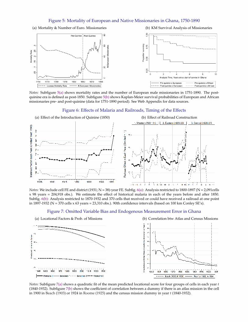
Figure 5: Mortality of European and Native Missionaries in Ghana, 1750-1890

(a) Mortality & Number of Euro. Missionaries (b) KM Survival Analysis of Missionaries

Notes: Subfigure 5(a) shows mortality rates and the number of European male missionaries in 1751-1890. The post-quinine era is defined as post-1850. Subfigure 5(b) shows Kaplan-Meier survival probabilities of European and Africanmissionaries pre- and post-quinine (data for 1751-1890 period). See Web Appendix for data sources.

Figure 6: Effects of Malaria and Railroads, Timing of the Effects

(a) Effect of the Introduction of Quinine (1850) (b) Effect of Railroad Construction

Notes: We include cell FE and district (1931; N = 38)-year FE. Subfig. 6(a): Analysis restricted to 1800-1897 (N = 2,091cellsx 98 years = 204,918 obs.). We estimate the effect of historical malaria in each of the years before and after 1850.Subfig. 6(b): Analysis restricted to 1870-1932 and 370 cells that received or could have received a railroad at one pointin 1897-1932 (N = 370 cells x 63 years = 23,310 obs.). 90th confidence intervals (based on 100 km Conley SE’s).

Figure 7: Omitted Variable Bias and Endogenous Measurement Error in Ghana

(a) Locational Factors & Prob. of Missions (b) Correlation btw Atlas and Census Missions

Notes: Subfigure 7(a) shows a quadratic fit of the mean predicted locational score for four groups of cells in each year t(1840-1932). Subfigure 7(b) shows the coefficient of correlation between a dummy if there is an atlas mission in the cellin 1900 in Beach (1903) or 1924 in Roome (1925) and the census mission dummy in year t (1840-1932).

40

Table 1: CORRELATES OF MISSIONARY EXPANSION, LONG-DIFF., SELECTED FACTORS

Dependent Variable: Dummy if Census Mission in the Cell in Selected Year:1850 1875 1897 1932

Variables of interest: (1) (2) (3) (4)

Dummy Any Census Mission .../1850/1875/1897 0.602*** 0.392*** 0.232***[0.082] [0.028] [0.058]

Historical Malaria Index -0.004* -0.005* 0.008 -0.010[0.002] [0.003] [0.006] [0.007]

Log Distance to Coast -0.017* -0.027** -0.035 -0.102***[0.009] [0.012] [0.021] [0.002]

Dummy if Port in the Cell 1850 0.166** 0.212*** 0.129 -0.159[0.080] [0.066] [0.093] [0.108]

Dummy if Outside Gold Coast Colony 1850 0.004 0.009 0.040 0.135**[0.010] [0.011] [0.045] [0.060]

Dummy if Navigable River 10 Km -0.024** -0.023* 0.037* 0.022[0.012] [0.012] [0.022] [0.029]

Dummy if Ashanti Trade Route 1850 10 Km 0.011 0.014** -0.004 0.006[0.008] [0.007] [0.009] [0.024]

Dummy if Non-Ashanti Trade Route 1850 10 Km 0.012** 0.012** 0.002 0.026[0.005] [0.005] [0.010] [0.018]

Dummy if Railroad 1932 10 Km -0.018** -0.017 0.067 0.079***[0.008] [0.010] [0.066] [0.018]

Log Urban Population 1891 0.015*** 0.026*** 0.008* 0.001[0.005] [0.007] [0.005] [0.002]

Log Urban Population 1901 -0.000 0.007** 0.024*** -0.011***[0.005] [0.003] [0.008] [0.003]

Log Urban Population 1931 0.001*** 0.000 0.017*** 0.032***[0.000] [0.002] [0.007] [0.011]

Log Rural Population 1901 0.001 0.001 0.007* 0.033***[0.001] [0.002] [0.004] [0.005]

Log Rural Population 1931 -0.001 -0.002 -0.002 0.016**[0.001] [0.001] [0.002] [0.007]

Dummy if Palm Oil Plantation 1900-1936 50 Km 0.018 0.029*** 0.089*** 0.082***[0.013] [0.011] [0.019] [0.016]

Dummy if Kola-Producing Cell 1932 -0.025* -0.017 0.042 0.073***[0.015] [0.016] [0.042] [0.019]

Dummy if Cocoa-Producing Cell 1927 0.006 0.008 0.073*** 0.096**[0.010] [0.009] [0.025] [0.041]

R-squared 0.35 0.61 0.50 0.61

Notes: For 2,091 cells and each period [t-s;t], we regress a dummy if there is a census mission in year t on a dummy if there is a censusmission in year t-s and various locational factors. We do not report the coefficients of land area, rainfall, altitude, ruggedness, soil fertility,four dummies if the cell contained a large pre-colonial city circa 1800, the largest or 2nd largest city in 1901, a headchief town in 1901, orthe central location of a mine in 1932, four dummies if the cell was within 10 km from a road in 1930, within 50 km from a slave marketc. 1800, within 50 km from a rubber plantation in 1900-1936, or was surveyed by the 1901 Population Census, and the log of normalizedslave exports in the 15th-19th Centuries. 100 km Conley SE’s: * p<0.10, ** p<0.05, *** p<0.01. See Web Appendix for data sources.

41

Table 2: MALARIA AND MISSIONARY EXPANSION, PANEL

Dep. Var.: Dummy if Census Mission in Cell c in Year t: (1800-1897) Missionary (1846-1890)Any Euro. Euro. Afri.

Any Resid.

Vars of interest: (1) (2) (3) (4) (5) (6) (7) (8) (9) (10) (11)

Malaria*1850-97 0.020*** 0.019*** 0.007*** 0.013*** 0.005*** 0.008*** 0.002*** 0.001*** 0.007***[0.001] [0.001] [0.001] [0.001] [0.001] [0.001] [0.001] [0.000] [0.001]

Malaria*1800-24 -0.002[0.001]

Malaria*1850-70 0.009*** 0.002***[0.001] [0.001]

Malaria*1870-97 0.028*** 0.011***[0.002] [0.002]

Cell FE Y Y Y Y Y Y Y Y Y Y YYear FE Y Y N Y N Y N Y Y Y YDistrict-Year FE N N Y N Y N Y N N N NGCC & Ashanti Ctrls N N N Y Y N N N N N N

Notes: (1)-(5): For 2,091 cells c and 98 years t (N = 204,918), we regress a dummy if there is a census mission in cell c in t on malariainteracted with a dummy if t is between 1850 and 1897. (8)-(11): For 2,091 cells c and 40 years t (N = 93,253), we regress a dummy ifthere is a missionary / Euro. missionary (“Resid.” indicates that the missionary lives there permanently instead of frequently visiting)/ African missionary in cell c in t on malaria interacted with a post-1850 dummy. 100 km Conley SE’s: * p<0.10, ** p<0.05, *** p<0.01.

Table 3: RAILROADS AND MISSIONARY EXPANSION, LONG-DIFFERENCES AND PANEL

Panel A: Dependent Variable: Dummy if Census Mission in 1932 (Incl. Controls and a Dummy if Census Mission in 1897)

Effect of Dummy Railroad 0-30 Km in 1932: Coeff. SE Obs. Controls

1. Baseline 0.162*** [0.033] 2,091 Y

2. Dep.Var.: Dummy Mission 1850, Ctrl Dummy Mission 1751 -0.015 [0.014] 2,091 Y3. Dep.Var.: Dummy Mission 1875, Ctrl Dummy Mission 1850 0.008 [0.020] 2,091 Y4. Dep.Var.: Dummy Mission 1897, Ctrl Dummy Mission 1875 0.031 [0.033] 2,091 Y

5. Including Ethnic Group Fixed Effects (N = 34) 0.180*** [0.022] 2,091 Y6. Including District in 1931 Fixed Effects (N = 38) 0.175*** [0.045] 2,091 Y

7. Railroad 0-30 Km Dummy Defined Using Western Line Only 0.140** [0.059]2,091 Y

Railroad 0-30 Km Dummy Defined Using Other Lines Only 0.174*** [0.025]

8. Railroad 0-30 Km Dummy Defined Using Existing Lines Only 0.176*** [0.041]2,091 Y

Railroad 0-30 Km Dummy Defined Using Placebo Lines Only 0.066 [0.055]

9. IV: 30 Km from Straight Lines (Drop Nodes; IV F=39) 0.230** [0.113] 2,088 Y

Panel B: Dependent Variable: Dummy if Census Mission in Year t (Including Cell Fixed Effects and Year Fixed Effects)

Effect of Dummy Railroad 0-30 Km in Year t: Coeff. SE Obs. Controls

10. Baseline Effect in Year t 0.179*** [0.019] 75,276 N

11. Effect of the Lead when Added 0.011 [0.035] 73,185 N

12. Baseline Effect in Year t if Adding 1 Lag 0.010 [0.036]73,185 N

Effect of the Lag 0.171*** [0.036]

13. Including Ethnic Group FE (N = 34) x Year FE (T = 36) 0.143*** [0.017] 75,276 N14. Including District in 1931 FE (N = 38) x Year FE (T = 36) 0.122*** [0.013] 75,276 N15. Including 2,091 Cell-Specific Linear Trends 0.173*** [0.036] 75,276 N

Notes: Panel A: For 2,091 cells, we regress a dummy if there is a mission in 1932 on a dummy if there is a mission in 1897 and variouscontrols (see text for details). Row 9: The IV is a dummy if the cell is within 30 Km from the straight lines Sekondi-Kumasi and Accra-Kumasi (three nodes dropped). Panel B: For 2,091 cells c and 36 years t (1897-1932), we regress a dummy if there is a mission in cell c int on a dummy if cell c is within 30 km of a railroad in t (cell FE & year FE incl.). 100 Km Conley SE’s (SE’s clust. at district (1931) level inrows 9 and 15 where Conley SEs are too computationally intensive): * p<0.10, ** p<0.05, *** p<0.01. See Web Appx. for data sources.

42

Table 4: CASH CROPS AND MISSIONARY EXPANSION, PANEL

Dependent Variable: Dummy if Census Mission in Year t (Including Cell Fixed Effects and Year Fixed Effects)

Effect of Log Predicted Cash Crop Export Value in Year t: Coeff. SE Obs.

1. Based on Palm Oil, Rubber, Kola & Cocoa Production 0.028*** [0.001] 181,917

2. Based on Contemporary Palm Oil & Cocoa Suitability 0.031*** [0.002] 181,9173. Based on Historical Palm Oil, Rubber & Cocoa Suitability 0.023*** [0.001] 181,917

4. Based on Palm Oil Production Only 0.031*** [0.005] 181,9175. Based on Rubber Production Only 0.020*** [0.001] 181,9176. Based on Kola Production Only 0.043*** [0.002] 181,9177. Based on Cocoa Production Only 0.042*** [0.001] 181,9178. Based on Historical Moderate, High & Very High Cocoa Suit. 0.029*** [0.001] 181,917

9. Overall Effect of Leads when Leads Added: 1 Lead -0.003 [0.005] 179,826

10. Baseline Effect in Year t when Lags Added: 1 Lag -0.001 [0.005] 179,826Overall Effect of Lags when Lags Added: 1 Lag 0.029*** [0.001]

11. Including Ethnic Group FE (N = 34) x Year FE (T = 87) 0.024*** [0.002] 181,91712. Including District in 1931 FE (N = 38) x Year FE (T = 87) 0.027*** [0.001] 181,91713. Including 2,091 Cell-Specific Linear Trends 0.024*** [0.006] 181,917

Notes: For 2,091 cells c and 87 years t (1846-1932), we regress a dummy if there is a mission in cell c in t on log predicted cash crop exportvalue in cell c in t (cell FE and year FE included). Rows 2-8: Using alternative ways to construct the predicted value of cash crop exports.100 Km Conley SE’s (clust. at district (1931) level in row 13): * p<0.10, ** p<0.05, *** p<0.01. See Web Appendix for data sources.

Table 5: RAILROADS, CASH CROPS AND MISSIONS, LONG-DIFF. AND PANEL, AFRICA

Panel A: Dependent Variable: Dummy if Atlas Mission ... (1) Defined in 1900 (2) Defined in 1924

Effect of Dummy Rail 0-30 Km ... Defined in 1900 Defined in 1924

Coeff. SE Coeff. SE

1. Rail 0-30 Km 0.007*** [0.002] 0.010*** [0.001]

2. Including Country-Ethnic Group Fixed Effects (N = 1,158) 0.008*** [0.002] 0.010*** [0.001]3. Including District ca 2000 Fixed Effects (N = 3,284) 0.007*** [0.003] 0.007*** [0.001]4. Rail 0-30 Km Dummy Using Military-Mining Lines Only 0.007*** [0.003] 0.006*** [0.002]5. IV: 30 Km from EMST Network (Drop Nodes; IV F = 49/82) 0.025** [0.011] 0.021*** [0.006]6. Rail 0-30 Km Dummy Using 1916 & 1922 Placebo Lines Only 0.001 [0.001] 0.001 [0.001]

Country FE, Controls of Table 6 except Pop, Crops, Roads t (see notes) Y Y Y Y

Panel B: Dependent Variable: Dummy if Atlas Mission ... (1) in Year t (2) in Year t

Effect of ... Rail 0-30 Km Dummy t Log Cash Crop t

Coeff. SE Coeff. SE

7. Baseline Effect in Year t 0.0027** [0.0011] 0.0011*** [0.0002]

8. Effect of the Lead when Added 0.0004 [0.0006] 0.0001 [0.0001]9. Baseline Effect in Year t if Lag Added 0.0028*** [0.0011] 0.0004*** [0.0001]

Effect of the Lag when Added -0.0007 [0.0013] 0.0009*** [0.0002]10. Including Ethnic-Year FE 0.0019* [0.0011] 0.0006** [0.0003]11. Including District-Year FE 0.0016 [0.0013] 0.0008** [0.0004]

Cell FE, Year FE, Country-year FE Y Y Y Y

Notes: Panel A: For 203,574 cells, we regress a dummy if there is an Atlas mission in 1900 (col. (1)) or 1924 (col. (2)) on the 0-30 Km raildummy and the controls of Table 6 except the population levels, cash crop and mining variables defined ca 1900 in col. (1) and ca 1924in col. (2) (see footnote 33 for details). Panel B Col. (1): For 103,866 cells c in 15 countries with railroads at one point in 1885-1990 andthe years 1885, 1890, 1895 and 1900 (N = 415,464), we regress a dummy if there is a mission in cell c in t on a dummy if cell c is within30 km of a railroad in t (cell FE, year FE, and country-year FE included). Panel B Col. (2): For 70,546 cells c in 20 countries with cashcrop export data and the years 1850, 1860, 1870, 1875, 1880, 1890 and 1900 (N = 493,822), we regress a dummy if there is a mission in cellc in t on log predicted cash crop export value in cell c in t (cell FE, year FE, and country-year FE included). See text for details on eachregression. Robust SE’s clustered at the district (2000) level: * p<0.10, **p<0.05, *** p<0.01. See Web Appx. for data sources.

43

Table 6: CORRELATES OF MISSIONS, LONG-DIFF. , SELECTED FACTORS, AFRICA

Dependent Variable: Columns (1)-(5) Dummy if Atlas Mission in the Cell in:Beach Roome Columns (3)-(5) Beach in ...

in 1900 in 1924 1850 1881 1900

(1) (2) (3) (4) (5)

Dummy if Any Mission in ... 1850 / 1881 0.9797*** 0.9866***[0.0037] [0.0019]

Historical Malaria Index -0.0254*** -0.0478*** -0.0039 -0.0147*** -0.0065[0.0094] [0.0157] [0.0029] [0.0046] [0.0063]

Tsetse Index -0.0033 -0.0085*** -0.0003 -0.0017 -0.0020[0.0023] [0.0028] [0.0007] [0.0012] [0.0013]

Log Distance to Coast -0.0030*** -0.0030*** -0.0007*** -0.0009*** -0.0015***[0.0005] [0.0005] [0.0002] [0.0002] [0.0003]

Dummy if Large Pre-Colonial City 1400 -0.0312*** 0.0502 -0.0082** -0.0134*** -0.0100***[0.0088] [0.0398] [0.0036] [0.0046] [0.0037]

Dummy if Largest or 2nd Largest City 1901 0.0579*** 0.1734*** 0.0264*** 0.0207 0.0297**[0.0196] [0.0265] [0.0095] [0.0140] [0.0145]

Year of Colonization -0.0000 -0.0000*** -0.0000** -0.0000 0.0000[0.0000] [0.0000] [0.0000] [0.0000] [0.0000]

Dummy if Centralized State (Murdock) 0.0023*** -0.0012* 0.0001 0.0012*** 0.0011***[0.0007] [0.0007] [0.0002] [0.0004] [0.0004]

Log Distance to Muslim Center -0.0006 0.0022*** 0.0004** -0.0002 -0.0005[0.0005] [0.0005] [0.0001] [0.0003] [0.0003]

Dummy if Slave Port in the Cell 1800-1900 0.0458** 0.1306*** 0.0121 0.0244 0.0071[0.0222] [0.0309] [0.0118] [0.0151] [0.0132]

Dummy if Navigable River 10 Km 0.0030** 0.0116*** -0.0004 -0.0004 0.0035***[0.0014] [0.0023] [0.0003] [0.0005] [0.0012]

Dummy if Explorer Route 10 Km 0.0006 0.0016* 0.0001 0.0002 0.0003[0.0006] [0.0008] [0.0001] [0.0004] [0.0005]

Dummy if Railroad 1900 / 1924 10 Km 0.0139*** 0.0227*** 0.0044** 0.0012 0.0046*[0.0043] [0.0027] [0.0020] [0.0023] [0.0024]

Log City Pop. ca 1900 (Loc.≥10,000) 0.0110*** 0.0024 0.0034** 0.0026 0.0041*[0.0029] [0.0029] [0.0017] [0.0019] [0.0021]

Log Urban Population 1900 0.0019*** 0.0065*** 0.0005*** 0.0009*** 0.0008***[0.0004] [0.0006] [0.0002] [0.0002] [0.0002]

Log Rural Population 1900 0.0008*** 0.0004** 0.0001** 0.0005*** 0.0002*[0.0002] [0.0002] [0.0001] [0.0001] [0.0001]

Dummy if Slavery (Murdock) 0.0011 0.0026*** 0.0002 0.0002 0.0006[0.0007] [0.0009] [0.0002] [0.0004] [0.0004]

Log Norm. Slave Exports 15th-19th Cent. 0.0009 0.0058*** -0.0001 0.0006 0.0006[0.0006] [0.0011] [0.0003] [0.0004] [0.0004]

Log Pred. Cash Crop Export Val. 1900 / 1924 0.0005*** 0.0005* 0.0002* 0.0003** 0.0001[0.0002] [0.0003] [0.0001] [0.0001] [0.0001]

Dummy if Polygamy (Murdock) -0.0015** 0.0013* -0.0000 -0.0010*** -0.0006[0.0006] [0.0007] [0.0001] [0.0004] [0.0004]

Fixed Effects Country Country Country Country CountryAdj. R-squared 0.03 0.04 0.02 0.25 0.52Notes: For 203,574 cells in 43 sub-Saharan African countries, we regress a dummy if there is an atlas mission in Beach in 1900 (col. (1)) or inRoome in 1924 (col. (2)) on various locational factors (country fixed effects always included). We do not report the coefficients of land area,rainfall, altitude, ruggedness, soil fertility, a dummy if there was a large pre-colonial city in the cell circa 1800, a dummy if the cell is within10 km from a lake, a dummy if the cell is within 50 km from a mine in 1900 or 1924, a dummy if the main ethnic group in the cell beforecolonization according to Murdock (1959) does not have information on state centralization, slavery and polygamy, a dummy if we knowthe year of the anthropological study used by Murdock (1959) to create his data, and a dummy if that year precedes 1900 / 1924. Col. (3)-(5): For Beach and each period [t-s;t], we regress a dummy if there is a mission in t on the locational factors and a dummy if there is amission in t-s. Robust SE’s clustered at the district (2000 boundaries) level: * p<0.10, ** p<0.05, *** p<0.01. See Web Appx. for data sources.

44

Table 7: CORRELATES OF BEACH (1900) AND ROOME (1924) MISSIONS, GHANA

Dependent Variable: Dummy if Any Atlas Mission in Cell c in...Col. (1)-(5): Beach in 1900 Col. (6)-(10): Roome in 1924

(1) (2) (3) (4) (5) (6) (7) (8) (9) (10)

Census Mission Year t 0.16*** 0.04*** -0.04 0.03** -0.05 0.06*** 0.01*** -0.07** 0.02* -0.01[0.03] [0.01] [0.05] [0.01] [0.05] [0.02] [0.00] [0.03] [0.01] [0.03]

Created 1751-1850 0.53*** 0.01 0.46*** 0.24*[0.05] [0.12] [0.14] [0.13]

Created 1851-1875 0.21*** -0.09** 0.22*** 0.12***[0.07] [0.04] [0.02] [0.02]

Log Num. Mis. Year t 0.06 0.06 0.22*** 0.17***[0.05] [0.04] [0.05] [0.05]

Main Station Year t 0.61*** 0.59*** 0.05* -0.01[0.11] [0.11] [0.03] [0.03]

School Year t 0.02 0.01 0.10* 0.09[0.03] [0.01] [0.06] [0.06]

Euro Resid 1846-90 0.08* 0.04** 0.01 -0.09**[0.05] [0.02] [0.03] [0.04]

Euro Visit 1846-90 0.40*** 0.10 0.37*** 0.10***[0.07] [0.11] [0.04] [0.04]

Observations 2091 2091 2091 2069 2069 2091 2091 2091 2069 2069R-squared 0.15 0.37 0.61 0.35 0.64 0.05 0.28 0.31 0.29 0.45

Notes: For 2,091 cells c, we regress a dummy if there is an atlas mission in cell c in Beach (1900) or Roome (1924) on the missioncharacteristics in the same cell the same year (1900 or 1924, unless otherwise indicated) in our census data. Col. (4)-(5) and (9)-(10):Identity of the missionary missing for 22 obs. 100 Km Conley SE’s: * p<0.10, ** p<0.05, *** p<0.01. See Web Appx for data sources.

Table 8: LONG-TERM ECONOMIC EFFECTS OF MISSIONS FOR MISSION MAP YEARS

Dependent Variable: Log Night Light Intensity in the Cell in 2010:

Controls Included: None Std Africa Ours +Type None Std Africa Ours +TypeEffect of ... Mission Dummy: (1) (2) (3) (4) (5) (6) (7) (8) (9) (10)

Panel A: Ghana (N = 2,091) Col. (1)-(5): 1900 (Beach, 1903) Col. (6)-(10): 1924 (Roome, 1925)

1. Census Mission Dummy 1.05*** 0.78*** 0.41*** 0.12 0.01 0.84*** 0.73*** 0.38*** 0.19*** 0.17***[0.13] [0.09] [0.08] [0.08] [0.03] [0.10] [0.07] [0.09] [0.05] [0.05]

2. Atlas Mission Dummy 1.76*** 1.39*** 0.78*** 0.54*** 0.44** 1.60*** 1.43*** 0.73*** 0.50*** 0.33**[0.20] [0.09] [0.15] [0.03] [0.19] [0.22] [0.10] [0.21] [0.15] [0.16]

Non-Atlas Mission Dummy 0.89*** 0.65*** 0.37*** 0.09 0.01 0.80*** 0.69*** 0.38*** 0.19*** 0.17***(= Census - Atlas Dummies) [0.10] [0.09] [0.10] [0.08] [0.03] [0.09] [0.07] [0.09] [0.05] [0.05]

3. Atlas Mission Dummy 1.67*** 1.22*** 0.59*** 0.48*** 0.43 1.40*** 1.08*** 0.43* 0.32* 0.16[0.21] [0.09] [0.22] [0.10] [0.26] [0.23] [0.12] [0.23] [0.17] [0.19]

Panel B: Africa (N = 203,574) Col. (1)-(5): 1900 (Beach, 1903) Col. (6)-(10): 1924 (Roome, 1925)

Atlas Mission Dummy 0.70*** 0.60*** 0.40*** 0.69*** 0.59*** 0.37***[0.05] [0.05] [0.04] [0.04] [0.04] [0.03]

Notes: Panel A: Ghana sample: 2,091 cells. Panel B: Africa sample: 203,574 cells in 43 sub-Saharan African countries. “Standard”:Controls identified as regularly used in the literature (see text for details). “Africa”: All Africa controls of Table 6. “Ours”: All Ghanacontrols of Table 1. “Type”: All Ghana controls of Table 7 except Log Num.Mis.Year t. 100 Km Conley SE’s for Ghana (Panel A) and SE’sclustered at the district (2000 boundaries) level for Africa (Panel B): * p<0.10, ** p<0.05, *** p<0.01. See Web Appendix for data sources.

45

Table 9: LONG-TERM EFFECTS OF MISSIONS DEPENDING ON THEIR TYPE, GHANA

Dependent Variable: Log Night Light Intensity in the Cell in 2010:

Dummies Defined in: Year 1900 (Same as Beach) Year 1924 (Same as Roome)

(1) (2) (3) (4) (5) (6) (7) (8)

Panel A: Standard Controls Included

Census Mission Year t 0.59*** 0.32** 0.56*** 0.26** 0.65*** 0.14 0.63*** 0.19[0.05] [0.16] [0.07] [0.11] [0.07] [0.12] [0.08] [0.12]

Created 1751-1850 0.65*** 0.27 0.77*** 0.10[0.08] [0.27] [0.06] [0.20]

Created 1851-1875 0.52*** 0.33* 0.60*** 0.25[0.11] [0.17] [0.06] [0.17]

Log Num. Mis. Year t 0.44*** 0.36*** 0.42*** 0.35***[0.09] [0.14] [0.07] [0.10]

Main Station Year t 0.23** -0.05 0.13 0.00[0.12] [0.14] [0.10] [0.13]

School Year t -0.08 -0.25** 0.18 0.17[0.12] [0.11] [0.12] [0.14]

Euro Resid 1846-1890 0.34** 0.24* 0.38*** 0.21***[0.15] [0.14] [0.09] [0.06]

Euro Visit 1846-1890 0.65*** 0.44** 0.74*** 0.30*[0.07] [0.21] [0.08] [0.17]

Panel B: Our Controls Included

Census Mission Year t 0.07 -0.15 0.01 -0.24*** 0.18*** 0.05 0.19*** 0.05[0.08] [0.12] [0.05] [0.09] [0.05] [0.10] [0.05] [0.08]

Created 1751-1850 0.35* 0.28 0.36* 0.25[0.20] [0.27] [0.20] [0.22]

Created 1851-1875 0.33*** 0.31** 0.34*** 0.31**[0.10] [0.15] [0.07] [0.15]

Log Num. Mis. Year t 0.36*** 0.33*** 0.13 0.13[0.10] [0.12] [0.10] [0.09]

Main Station Year t 0.09 -0.08 0.03 -0.01[0.10] [0.07] [0.09] [0.09]

School Year t -0.23** -0.24*** 0.06 0.11[0.14] [0.08] [0.06] [0.08]

Euro Resid 1846-1890 0.23*** 0.15 0.19*** 0.09[0.08] [0.12] [0.07] [0.11]

Euro Visit 1846-1890 0.31*** 0.18 0.29*** 0.09[0.06] [0.17] [0.07] [0.16]

Observations 2,091 2,091 2,069 2,069 2,091 2,091 2,069 2,069

Notes: For 2,069-2,091 cells in Ghana (note that the identity of the missionary is missing for 2,091 - 2,069 = 22 obs.), we regress ourmain measure of local economic development, log mean night light intensity in the cell in 2010, on the census mission dummyand mission characteristics in the cell, all defined in the same year (1900 / 1924). Panel A: Standard Controls: Controls identifiedas regularly used in the literature (see text for details). Panel B: Our controls: All controls of Table 1. “Euro Resid 1846-1890”:Mission stations where European missionaries permanently resided at one point in 1846-1890 (data not available for other years).“Euro Visit 1846-1890”: Mission stations where European missionaries did not permanently reside but frequently visited at onepoint in 1846-1890. Robust 100 km Conley SE’s: * p<0.10, ** p<0.05, *** p<0.01. See Web Appendix for data sources.