Embed Size (px)
Citation preview
http://www.econometricsociety.org/
Econometrica, Vol. 83, No. 6 (November, 2015), 2127–2189
THE ECONOMICS OF DENSITY:EVIDENCE FROM THE BERLIN WALL
GABRIEL M. AHLFELDTLondon School of Economics, London, WC2A 2AE, U.K. and CEPR
STEPHEN J. REDDINGWWS, Princeton University, Princeton, NJ 08540, U.S.A., NBER, and CEPR
DANIEL M. STURMLondon School of Economics, London, WC2A 2AE, U.K. and CEPR
NIKOLAUS WOLFHumboldt University, 10178 Berlin, Germany and CEPR
The copyright to this Article is held by the Econometric Society. It may be downloaded,printed and reproduced only for educational or research purposes, including use in coursepacks. No downloading or copying may be done for any commercial purpose without theexplicit permission of the Econometric Society. For such commercial purposes contactthe Office of the Econometric Society (contact information may be found at the websitehttp://www.econometricsociety.org or in the back cover of Econometrica). This statement mustbe included on all copies of this Article that are made available electronically or in any otherformat.
Econometrica, Vol. 83, No. 6 (November, 2015), 2127–2189
THE ECONOMICS OF DENSITY:EVIDENCE FROM THE BERLIN WALL
BY GABRIEL M. AHLFELDT, STEPHEN J. REDDING,DANIEL M. STURM, AND NIKOLAUS WOLF1
This paper develops a quantitative model of internal city structure that featuresagglomeration and dispersion forces and an arbitrary number of heterogeneous cityblocks. The model remains tractable and amenable to empirical analysis because ofstochastic shocks to commuting decisions, which yield a gravity equation for commut-ing flows. To structurally estimate agglomeration and dispersion forces, we use data onthousands of city blocks in Berlin for 1936, 1986, and 2006 and exogenous variationfrom the city’s division and reunification. We estimate substantial and highly localizedproduction and residential externalities. We show that the model with the estimatedagglomeration parameters can account both qualitatively and quantitatively for theobserved changes in city structure. We show how our quantitative framework can beused to undertake counterfactuals for changes in the organization of economic activitywithin cities in response, for example, to changes in the transport network.
KEYWORDS: Agglomeration, cities, commuting, density, gravity.
1. INTRODUCTION
ECONOMIC ACTIVITY IS HIGHLY UNEVENLY DISTRIBUTED across space, as re-flected in the existence of cities and the concentration of economic functions inspecific locations within cities, such as Manhattan in New York and the SquareMile in London. Understanding the strength of the agglomeration and disper-sion forces that underlie these concentrations of economic activity is centralto a range of economic and policy questions. These forces shape the size andinternal structure of cities, with implications for the incomes of immobile fac-tors, congestion costs, and city productivity. They also determine the impactof public policy interventions, such as transport infrastructure investments andurban development and taxation policies.
1We are grateful to the European Research Council (Grant 263733), German Science Foun-dation (Grants STU 477/1-1 and WO 1429/1-1), the Centre for Economic Performance, andPrinceton University for financial support. The accompanying online Supplemental Material con-tains detailed derivations and supplementary material for the paper. A separate Technical DataAppendix, located together with the replication data and code, collects together additional em-pirical results and robustness tests. Thilo Albers, Horst Bräunlich, Daniela Glocker, KristofferMöller, David Nagy, Utz Pape, Ferdinand Rauch, Claudia Steinwender, Sevrin Waights, andNicolai Wendland provided excellent research assistance. We would like to thank the editor, fouranonymous referees, conference and seminar participants at AEA, Arizona, Barcelona, Berlin,Berkeley, Brussels, CEPR, Chicago, Clemson, Columbia, EEA, Harvard, Mannheim, Marseille,MIT, Munich, NARSC, Luzern, Nottingham, NYU, Oxford, Paris, Princeton, Rutgers, Shanghai,Stanford, Tübingen, UCLA, Virginia, and the World Bank for helpful comments. We are alsograteful to Dave Donaldson, Cecilia Fieler, Gene Grossman, Bo Honore, Ulrich Müller, SamKortum, Eduardo Morales, and Esteban Rossi-Hansberg for their comments and suggestions.The usual disclaimer applies.
© 2015 The Econometric Society DOI: 10.3982/ECTA10876
2128 AHLFELDT, REDDING, STURM, AND WOLF
Although there is a long literature on economic geography and urban eco-nomics dating back to at least Marshall (1920), a central challenge remainsdistinguishing agglomeration and dispersion forces from variation in locationalfundamentals. While high land prices and levels of economic activity in a groupof neighboring locations are consistent with strong agglomeration forces, theyare also consistent with shared amenities that make these locations attractiveplaces to live (e.g., leafy streets and scenic views) or common natural advan-tages that make these locations attractive for production (e.g., access to naturalwater). This challenge has both theoretical and empirical dimensions. From atheoretical perspective, to develop tractable models of cities, the existing liter-ature typically makes simplifying assumptions such as monocentricity or sym-metry, which abstracts from variation in locational fundamentals and limitsthe usefulness of these models for empirical work. From an empirical perspec-tive, the challenge is to find exogenous sources of variation in the surroundingconcentration of economic activity to help disentangle agglomeration and dis-persion forces from variation in locational fundamentals.
In this paper, we develop a quantitative theoretical model of internal citystructure. This model incorporates agglomeration and dispersion forces and anarbitrary number of heterogeneous locations within the city, while remainingtractable and amenable to empirical analysis. Locations differ in terms of pro-ductivity, amenities, the density of development (which determines the ratio offloor space to ground area), and access to transport infrastructure. Productivitydepends on production externalities, which are determined by the surround-ing density of workers, and production fundamentals, such as topography andproximity to natural supplies of water. Amenities depend on residential ex-ternalities, which are determined by the surrounding density of residents, andresidential fundamentals, such as access to forests and lakes. Congestion forcestake the form of an inelastic supply of land and commuting costs that are in-creasing in travel time, where travel time in turn depends on the transportnetwork.2
We combine this quantitative theoretical model with the natural experimentof Berlin’s division in the aftermath of the Second World War and its reuni-fication following the fall of the Iron Curtain. The division of Berlin severedall local economic interactions between East and West Berlin, which corre-sponds in the model to prohibitive trade and commuting costs and no produc-tion and residential externalities between these two parts of the city. We makeuse of a remarkable and newly collected data set for Berlin, which includesdata on land prices, employment by place of work (which we term “workplaceemployment”), and employment by place of residence (which we term “resi-dence employment”) covering the pre-war, division, and reunification periods.
2We use “production fundamental” to refer to a characteristic of a location that directly affectsproductivity (e.g., natural water) independently of the surrounding economic activity. We use“residential fundamental” to refer to a characteristic of a location that directly affects the utilityof residents (e.g., forests) independently of the surrounding economic activity.
THE ECONOMICS OF DENSITY 2129
We first present reduced-form evidence in support of the model’s qualitativepredictions without imposing the full structure of the model. We show that di-vision leads to a reorientation of the gradient in land prices and employmentin West Berlin away from the main pre-war concentration of economic activityin East Berlin, while reunification leads to a reemergence of this gradient. Incontrast, there is little effect of division or reunification on land prices or em-ployment along other more economically remote sections of the Berlin Wall.We show that these results are not driven by pre-trends prior to division orreunification. We also show that these results are robust to controlling for ahost of observable block characteristics, including controls for access to thetransport network, schools, parks and other green areas, lakes and other waterareas, Second World War destruction, land use, urban regeneration policies,and government buildings post reunification.
We next examine whether the model can account quantitatively for the ob-served impact of division and reunification. We show that the model implies agravity equation for commuting flows, which can be used to estimate its com-muting parameters. Using these estimates, we determine overall measures ofproductivity, amenities, and the density of development for each block, with-out making any assumptions about the relative importance or functional formof externalities and fundamentals as components of overall productivity andamenities. In the special case of the model in which overall productivity andamenities are exogenous, the model has a unique equilibrium, and hence canbe used to undertake counterfactuals that have determinate predictions forthe impact of division and reunification. We use these counterfactuals to showthat the model with exogenous productivity and amenities is unable to accountquantitatively for the observed impact of division and reunification on the pat-tern of economic activity within West Berlin.
We next use the exogenous variation from Berlin’s division and reunifica-tion to structurally estimate both the agglomeration and commuting parame-ters. This allows us to decompose overall productivity and amenities for eachblock into production and residential externalities (which capture agglomer-ation forces) and production and residential fundamentals (which are struc-tural residuals). Our identifying assumption is that changes in these structuralresiduals are uncorrelated with the exogenous change in the surrounding con-centration of economic activity induced by Berlin’s division and reunification.This identifying assumption requires that the systematic change in the patternof economic activity in West Berlin following division and reunification is ex-plained by the mechanisms of the model (the changes in commuting access andproduction and residential externalities) rather than by systematic changes inthe pattern of structural residuals (production and residential fundamentals).
Our structural estimates of the model’s parameters imply substantial andhighly localized production externalities. Our central estimate of the elasticityof productivity with respect to the density of workplace employment is 0.07,which is towards the high end of the range of existing estimates using variation
2130 AHLFELDT, REDDING, STURM, AND WOLF
between cities. In contrast to these existing estimates using data across cities,our analysis makes use of variation within cities. Our structural estimate ofthe elasticity of productivity with respect to density holds constant the distri-bution of travel times within the city. In reality, a doubling in total city pop-ulation is typically achieved by a combination of an increase in the density ofeconomic activity and an expansion in geographical land area, which increasestravel times within the city. Since we find that production externalities decayrapidly with travel times, this attenuates production externalities, which has tobe taken into account when comparing estimates within and across cities. Wealso find substantial and highly localized residential externalities. Our centralestimate of the elasticity of amenities with respect to the density of residentsis 0.15, which is consistent with the view that consumption externalities are animportant agglomeration force in addition to production externalities.
In the presence of agglomeration forces, there is the potential for multipleequilibria in the model. An advantage of our estimation approach is that it ad-dresses this potential existence of multiple equilibria. We distinguish betweencalibrating the model to the observed data given known parameter values andestimating the model for unknown parameters. First, given known values forthe model’s parameters, we show that there is a unique mapping from theseparameters and the observed data to the structural residuals (production andresidential fundamentals). This mapping is unique regardless of whether themodel has a single equilibrium or multiple equilibria, because the parameters,observed data, and equilibrium conditions of the model (including profit max-imization, zero profits, utility maximization, and population mobility) containenough information to solve for unique values of these structural residuals.Second, we estimate the model’s parameters using the generalized method ofmoments (GMM) and moment conditions in terms of these structural residu-als. Since these structural residuals are closed-form functions of the observeddata and parameters, this estimation holds constant the observed endogenousvariables of the model at their values in the data. In principle, these momentconditions need not uniquely identify the model parameters, because the ob-jective function defined by them may not be globally concave. For example,the objective function could be flat in the parameter space or there could bemultiple local minima corresponding to different combinations of parametersand unobserved fundamentals that explain the data. In practice, we show thatthe objective function is well behaved in the parameter space, and that thesemoment conditions determine a unique value for the parameter vector.
We also undertake counterfactuals in the estimated model with agglomer-ation forces. To address the potential for multiple equilibria in this case, weassume the equilibrium selection rule of searching for the counterfactual equi-librium closest to the observed equilibrium prior to the counterfactual. Weshow that the model with the estimated agglomeration parameters can gener-ate counterfactual predictions for the treatment effects of division and reunifi-cation that are close to the observed treatment effects. We also show how our
THE ECONOMICS OF DENSITY 2131
quantitative framework can be used to undertake counterfactuals for changesin the organization of economic activity within cities in response, for example,to changes in the transport network.
Finally, we undertake a variety of over-identification checks and robustnesstests. First, using our estimates of the model’s commuting parameters basedon bilateral commuting flows for 2008, we show that the model is successfulin capturing the cumulative distribution of commuters across travel times inthe pre-war, division, and reunification periods. Second, we find that the ratioof floor space to land area in the model is strongly related to separate dataon this variable not used in the estimation of the model. Finally, we also findthat production and residential fundamentals in the model are correlated inthe expected way with observable proxies for these fundamentals.
Our paper builds on the large theoretical literature on urban economics.Much of this literature has analyzed the monocentric city model, in which firmsare assumed to locate in a Central Business District (CBD) and workers decidehow close to live to this CBD.3 Lucas and Rossi-Hansberg (2002) were the firstto develop a model of a two-dimensional city, in which equilibrium patterns ofeconomic activity can be nonmonocentric. In their model, space is continuousand the city is assumed to be symmetric, so that distance from the center isa summary statistic for the organization of economic activity within the city.4Empirically, cities are, however, not perfectly symmetric because of variationin locational fundamentals, and most data on cities are reported for discretespatial units such as blocks or census tracts.
Our contribution is to develop a quantitative theoretical model of internalcity structure that allows for a large number of discrete locations within the citythat can differ arbitrarily in terms of their natural advantages for production,residential amenities, land supply, and transport infrastructure. The analysisremains tractable despite the large number of asymmetric locations becausewe incorporate a stochastic formulation of workers’ commuting decisions thatfollows Eaton and Kortum (2002) and McFadden (1974). This stochastic for-mulation yields a system of equations that can be solved for unique equilibriumwages given observed workplace and residence employment in each location.It also provides microeconomic foundations for a gravity equation for com-muting flows that has been found to be empirically successful.5
Our paper is also related to the broader literature on the nature and sourcesof agglomeration economies, as reviewed in Duranton and Puga (2004) andRosenthal and Strange (2004). A large empirical literature has regressed
3The classic urban models of Alonso (1964), Mills (1967), and Muth (1969) assume monocen-tricity. While Fujita and Ogawa (1982) and Fujita and Krugman (1995) allowed for nonmonocen-tricity, they modeled one-dimensional cities on the real line.
4For an empirical analysis of the symmetric-city model of Lucas and Rossi-Hansberg (2002),see Brinkman (2013).
5See Grogger and Hanson (2011) and Kennan and Walker (2011) for analyses of worker mi-gration decisions using stochastic formulations of utility following McFadden (1974).
2132 AHLFELDT, REDDING, STURM, AND WOLF
wages, land prices, productivity, or employment growth on population den-sity.6 We contribute to the small strand of research within this literature thathas sought sources of exogenous variation in the surrounding concentration ofeconomic activity. For example, Rosenthal and Strange (2008) and Combes,Duranton, Gobillon, and Roux (2010) used geology as an instrument for pop-ulation density, exploiting the idea that tall buildings are easier to constructwhere solid bedrock is accessible. Greenstone, Hornbeck, and Moretti (2010)provided evidence on agglomeration spillovers by comparing changes in totalfactor productivity (TFP) among incumbent plants in “winning” counties thatattracted a large manufacturing plant and “losing” counties that were the newplant’s runner-up choice.7
Other related research has examined the effect of historical natural exper-iments on the location of economic activity, including Hanson (1996, 1997)using Mexican trade liberalization; Davis and Weinstein (2002, 2008) using thewartime bombing of Japan; Bleakley and Lin (2012) using historical portagesites; and Kline and Moretti (2014) using the Tennessee Valley Authority(TVA). Using the division and reunification of Germany, Redding and Sturm(2008) examined the effect of changes in market access on the growth of WestGerman cities, and Redding, Sturm, and Wolf (2011) examined the reloca-tion of Germany’s air hub from Berlin to Frankfurt as a shift between multiplesteady-states. In contrast to all of the above studies, which exploit variationacross regions or cities, our focus is on the determinants of economic activ-ity within cities.8 Our main contribution is to develop a tractable quantitativemodel of internal city structure that incorporates agglomeration forces and arich geography of heterogeneous location characteristics and structurally esti-mate the model using the exogenous variation of Berlin’s division and reunifi-cation.
The remainder of the paper is structured as follows. Section 2 discussesthe historical background. Section 3 outlines the model. Section 4 introducesour data. Section 5 presents reduced-form empirical results on the impact ofBerlin’s division and reunification. Section 6 uses the model’s gravity equationpredictions to determine the commuting parameters and solve for overall val-ues of productivity, amenities, and the density of development. Section 7 struc-turally estimates both the model’s agglomeration and commuting parameters;
6See, for example, Ciccone and Hall (1996), Dekle and Eaton (1999), Glaeser and Mare(2001), Henderson, Kuncoro, and Turner (1995), Moretti (2004), Rauch (1993), Roback (1982),and Sveikauskas (1975), as surveyed in Moretti (2011).
7Another related empirical literature has examined the relationship between economic activ-ity and transport infrastructure, including Donaldson (2015), Baum-Snow (2007), Duranton andTurner (2012), Faber (2015), and Michaels (2008).
8Other research using within-city data includes Arzaghi and Henderson (2008) on the locationof advertising agencies in Manhattan and Rossi-Hansberg, Sarte, and Owens (2010) on urbanrevitalization policies in Richmond, Virginia.
THE ECONOMICS OF DENSITY 2133
uses these estimated parameters to decompose overall productivity and ameni-ties into the contributions of externalities and fundamentals; and undertakescounterfactuals. Section 8 concludes.
2. HISTORICAL BACKGROUND
The city of Berlin in its current boundaries was created in 1920 whenthe historical city and its surrounding agglomeration were incorporated un-der the Greater Berlin law (“Gross Berlin Gesetz”). The city comprises 892square kilometers of land compared, for example, to 606 square kilometers forChicago. The city was originally divided into 20 districts (“Bezirke”), which hadminimal administrative autonomy.9 The political process that ultimately led tothe construction of the Berlin Wall had its origins in war-time planning dur-ing the Second World War. A protocol signed in London in September 1944delineated zones of occupation in Germany for the American, British, and So-viet armies after the eventual defeat of Germany. This protocol also stipulatedthat Berlin, although around 200 kilometers within the Soviet occupation zone,should be jointly occupied. For this purpose, Berlin was itself divided into sep-arate occupation sectors.
The key principles underlying the drawing of the boundaries of the occupa-tion sectors in Berlin were that the sectors should be geographically orientatedto correspond with the occupation zones (with the Soviets in the East and theWestern Allies in the West); the boundaries between them should respect theboundaries of the existing administrative districts of Berlin; and the Ameri-can, British, and Soviet sectors should be approximately equal in population(prior to the creation of the French sector from part of the British sector).The final agreement in July 1945 allocated six districts to the American sector(31 percent of the 1939 population and 24 percent of the area), four districtsto the British sector (21 percent of the 1939 population and 19 percent of thearea), two districts to the French sector (12 percent of the 1939 population and12 percent of the area), and eight districts to the Soviet sector (37 percent ofthe 1939 population and 46 percent of the area).10
The London protocol specifying the occupation sectors also created institu-tions for a joint administration of Berlin (and Germany more generally). The
9The boundaries of these 20 districts were slightly revised in April 1938. During division,the East Berlin authorities created three new districts (Hellersdorf, Marzahn, and Hohenschön-hausen), which were created from parts of Weissensee and Lichtenberg. Except for a few otherminor changes, as discussed in Elkins and Hofmeister (1988), the district boundaries remainedunchanged during the post-war period until an administrative reform in 2001, which reduced thenumber of districts to twelve.
10The occupation sectors were based on the April 1938 revision of the boundaries of the 20pre-war districts. For further discussion of the diplomatic history of the division of Berlin, seeFranklin (1963) and Sharp (1975).
2134 AHLFELDT, REDDING, STURM, AND WOLF
intention was for Berlin to be governed as a single economic and administra-tive unit by a joint council (“Kommandatura”) with Soviet, American, British,and French representatives. However, with the onset of the Cold War, the rela-tionship between the Western allies and the Soviet Union began to deteriorate.In June 1948, the Western allies unilaterally introduced a new currency in theiroccupation zones and the Western sectors of Berlin. In retaliation, the SovietUnion decided to block all road and rail access to the Western sectors of Berlinfor nearly eleven months, and West Berlin was supplied through the Berlin air-lift during this time. The foundation of East and West Germany as separatestates in 1949 and the creation of separate city governments in East and WestBerlin further cemented the division of Germany and Berlin into Eastern andWestern parts.
Following the adoption of Soviet-style policies of command and control inEast Germany, the main border between East and West Germany was closedin 1952. While the implementation of these policies in East Berlin limited eco-nomic interactions with the Western sectors, the boundary between East andWest Berlin remained formally open.11 This open border resulted in some com-muting of workers between East and West Berlin.12 It also became a conduitfor refugees fleeing to West Germany. To stem this flow of refugees, the EastGerman authorities constructed the Berlin Wall in 1961, which ended all localeconomic interactions between East and West Berlin.
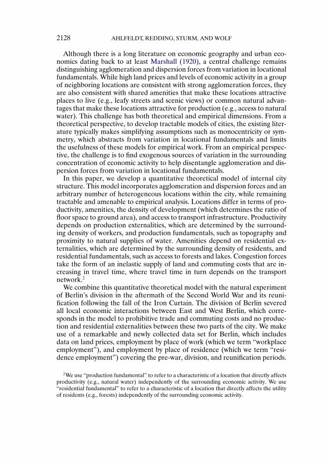
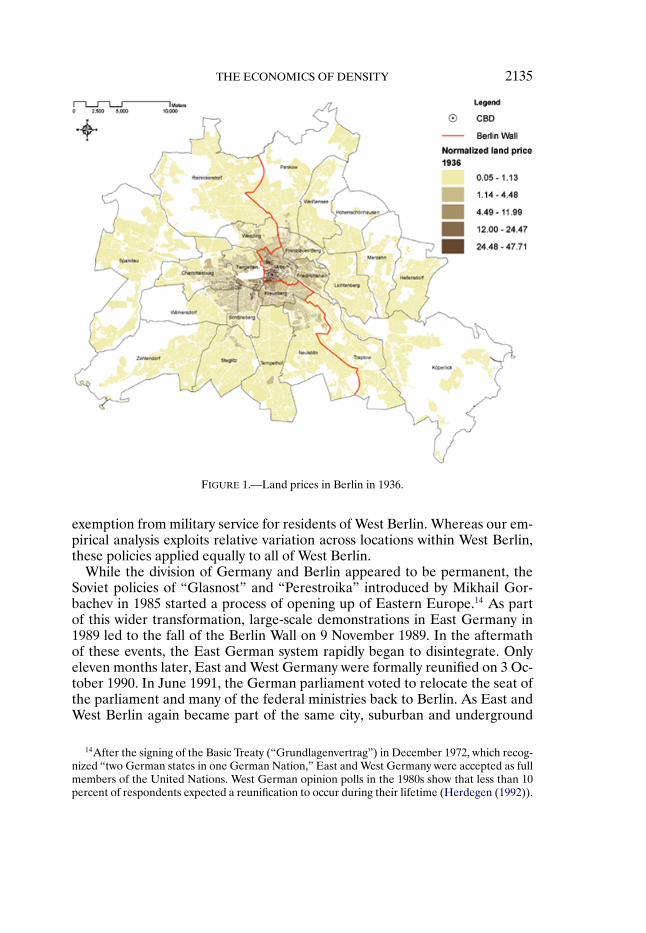
Figure 1 shows the pre-war land price gradient in Berlin and the path of theBerlin Wall. As apparent from the figure, the Berlin Wall consisted of an in-ner boundary between West and East Berlin and an outer boundary betweenWest Berlin and East Germany. The inner boundary ran along the Westernedge of the district Mitte, which contained Berlin’s main administrative, cul-tural, and educational institutions and by far the largest pre-war concentrationof employment. The Berlin Wall cut through the pre-war transport network, in-tersecting underground railway (“U-Bahn”) and suburban railway (“S-Bahn”)lines, which were closed off at the boundaries with East Berlin or East Ger-many.13 During the period of division, West Germany introduced a number ofpolicies to support economic activity in West Berlin, such as subsidies to trans-portation between West Berlin and West Germany, reduced tax rates, and an
11While East Berlin remained the main concentration of economic activity in East Germanyafter division, only around 2 percent of West Berlin’s exports from 1957 to 1967 were to EastGermany (including East Berlin) and other Eastern block countries (see Lambrecht and Tischner(1969)).
12Approximately 122,000 people commuted from West to East Berlin in the fall of 1949, butthis number quickly declined after waves of mass redundancies of Western workers in East Berlinand stood at about 13,000 workers in 1961 just before the construction of the Berlin Wall. Com-muting flows in the opposite direction are estimated to be 76,000 in 1949 and decline to 31,000 in1953 before slowly climbing to 63,000 in 1961 (Roggenbuch (2008)).
13In a few cases, trains briefly passed through East Berlin territory en route from one partof West Berlin to another. These cases gave rise to ghost stations (“Geisterbahnhöfe”) in EastBerlin, where trains passed through stations patrolled by East German guards without stopping.
THE ECONOMICS OF DENSITY 2135
FIGURE 1.—Land prices in Berlin in 1936.
exemption from military service for residents of West Berlin. Whereas our em-pirical analysis exploits relative variation across locations within West Berlin,these policies applied equally to all of West Berlin.
While the division of Germany and Berlin appeared to be permanent, theSoviet policies of “Glasnost” and “Perestroika” introduced by Mikhail Gor-bachev in 1985 started a process of opening up of Eastern Europe.14 As partof this wider transformation, large-scale demonstrations in East Germany in1989 led to the fall of the Berlin Wall on 9 November 1989. In the aftermathof these events, the East German system rapidly began to disintegrate. Onlyeleven months later, East and West Germany were formally reunified on 3 Oc-tober 1990. In June 1991, the German parliament voted to relocate the seat ofthe parliament and many of the federal ministries back to Berlin. As East andWest Berlin again became part of the same city, suburban and underground
14After the signing of the Basic Treaty (“Grundlagenvertrag”) in December 1972, which recog-nized “two German states in one German Nation,” East and West Germany were accepted as fullmembers of the United Nations. West German opinion polls in the 1980s show that less than 10percent of respondents expected a reunification to occur during their lifetime (Herdegen (1992)).
2136 AHLFELDT, REDDING, STURM, AND WOLF
rail lines and utility networks were rapidly reconnected. The reunification ofthe city was also accompanied by some urban regeneration initiatives and weinclude controls for these policies in our empirical analysis below.
3. THEORETICAL MODEL
To guide our empirical analysis, we develop a model in which the internalstructure of the city is driven by a tension between agglomeration forces (inthe form of production and residential externalities) and dispersion forces (inthe form of commuting costs and an inelastic supply of land).15
We consider a city embedded within a wider economy. The city consists ofa set of discrete locations or blocks, which are indexed by i = 1� � � � � S. Eachblock has an effective supply of floor space Li. Floor space can be used com-mercially or residentially, and we denote the endogenous fractions of floorspace allocated to commercial and residential use by θi and 1−θi, respectively.
The city is populated by an endogenous measure ofH workers, who are per-fectly mobile within the city and the larger economy, which provides a reser-vation level of utility U . Workers decide whether or not to move to the citybefore observing idiosyncratic utility shocks for each possible pair of residenceand employment blocks within the city. If a worker decides to move to the city,he or she observes these realizations for idiosyncratic utility, and picks the pairof residence and employment blocks within the city that maximizes his or herutility. Firms produce a single final good, which is costlessly traded within thecity and the larger economy, and is chosen as the numeraire (p= 1).16
Blocks differ in terms of their final goods productivity, residential amenities,supply of floor space, and access to the transport network, which determinestravel times between any two blocks in the city. We first develop the model withexogenous values of these location characteristics, before introducing endoge-nous agglomeration forces below.
3.1. Workers
Workers are risk neutral and have preferences that are linear in a consump-tion index: Uijo = Cijo, where Cijo denotes the consumption index for workero residing in block i and working in block j.17 This consumption index de-
15A more detailed discussion of the model and the technical derivations of all expressions andresults reported in this section are contained in the Supplemental Material (Ahlfeldt, Redding,Sturm, and Wolf (2015)).
16We follow the canonical urban model in assuming a single tradable final good and examinethe ability of this canonical model to account quantitatively for the observed impact of divisionand reunification, though the model can be extended to allow for the consumption of nontradedgoods by both workplace and residence.
17To simplify the exposition, throughout the paper, we index a worker’s block of residence by ior r and her block of employment by j or s unless otherwise indicated.
THE ECONOMICS OF DENSITY 2137
pends on consumption of the single final good (cijo); consumption of residen-tial floor space (�ijo); residential amenities (Bi) that capture common charac-teristics that make a block a more or less attractive place to live (e.g., leafystreets and scenic views); the disutility from commuting from residence blocki to workplace block j (dij ≥ 1); and an idiosyncratic shock that is specific toindividual workers and varies with the worker’s blocks of employment and res-idence (zijo). This idiosyncratic shock captures the idea that individual workerscan have idiosyncratic reasons for living and working in different parts of thecity. In particular, the aggregate consumption index is assumed to take theCobb–Douglas form:18
Cijo = Bizijo
dij
(cijo
β
)β(�ijo
1 −β)1−β
� 0<β< 1�(1)
where the iceberg commuting cost dij = eκτij ∈ [1�∞) increases with the traveltime (τij) between blocks i and j. Travel time is measured in minutes and iscomputed based on the transport network, as discussed further in Section 4below. The parameter κ controls the size of commuting costs.
We model the heterogeneity in the utility that workers derive from living andworking in different parts of the city following McFadden (1974) and Eatonand Kortum (2002). For each worker o living in block i and commuting to blockj, the idiosyncratic component of utility (zijo) is drawn from an independentFréchet distribution:
F(zijo)= e−TiEjz−εijo � Ti�Ej > 0� ε > 1�(2)
where the scale parameter Ti > 0 determines the average utility derived fromliving in block i; the scale parameter Ej determines the average utility derivedfrom working in block j; and the shape parameter ε > 1 controls the dispersionof idiosyncratic utility.
After observing her realizations for idiosyncratic utility for each pair of res-idence and employment blocks, each worker chooses where to live and workto maximize her utility, taking as given residential amenities, goods prices, fac-tor prices, and the location decisions of other workers and firms. Therefore,workers sort across pairs of residence and employment blocks depending ontheir idiosyncratic preferences and the characteristics of these locations. Theindirect utility from residing in block i and working in block j can be expressedin terms of the wage paid at this workplace (wj), commuting costs (dij), the
18For empirical evidence using U.S. data in support of the constant housing expenditure shareimplied by the Cobb–Douglas functional form, see Davis and Ortalo-Magné (2011). The roleplayed by residential amenities in influencing utility is emphasized in the literature followingRoback (1982). See Albouy (2008) for a recent prominent contribution.
2138 AHLFELDT, REDDING, STURM, AND WOLF
residential floor price (Qi), the common component of amenities (Bi), and theidiosyncratic shock (zijo):19
uijo = zijoBiwjQβ−1i
dij�(3)
where we have used utility maximization and the choice of the final good asnumeraire.
Although we model commuting costs in terms of utility, there is an isomor-phic formulation in terms of a reduction in effective units of labor, becausethe iceberg commuting cost dij = eκτij enters the indirect utility function (3)multiplicatively. As a result, commuting costs are proportional to wages, andthis specification captures changes over time in the opportunity cost of traveltime. Similarly, although we model the heterogeneity in commuting decisionsin terms of an idiosyncratic shock to preferences, there is an isomorphic inter-pretation in terms of a shock to effective units of labor, because this shock zijoenters indirect utility (3) multiplicatively with the wage.
Since indirect utility is a monotonic function of the idiosyncratic shock (zijo),which has a Fréchet distribution, it follows that indirect utility for workers liv-ing in block i and working in block j also has a Fréchet distribution. Eachworker chooses the bilateral commute that offers her the maximum utility,where the maximum of Fréchet distributed random variables is itself Fréchetdistributed. Using these distributions of utility, the probability that a workerchooses to live in block i and work in block j is
πij = TiEj(dijQ
1−βi
)−ε(Biwj)
ε
S∑r=1
S∑s=1
TrEs(drsQ
1−βr
)−ε(Brws)
ε
≡ Φij
Φ�(4)
Summing these probabilities across workplaces for a given residence, we ob-tain the overall probability that a worker resides in block i (πRi), while sum-ming these probabilities across residences for a given workplace, we obtain theoverall probability that a worker works in block j (πMi):
πRi =S∑j=1
πij =
S∑j=1
Φij
Φ� πMj =
S∑i=1
πij =
S∑i=1
Φij
Φ�(5)
19We make the standard assumption in the urban literature that income from land is accruedby absentee landlords and not spent within the city, although it is also possible to consider thecase where it is redistributed lump sum to workers.
THE ECONOMICS OF DENSITY 2139
These residential and workplace choice probabilities have an intuitive inter-pretation. The idiosyncratic shock to preferences zijo implies that individualworkers choose different bilateral commutes when faced with the same prices{Qi�wj}, commuting costs {dij}, and location characteristics {Bi�Ti�Ej}. Otherthings equal, workers are more likely to live in block i, the more attractive itsamenities Bi, the higher its average idiosyncratic utility as determined by Ti,the lower its residential floor prices Qi, and the lower its commuting costs dijto employment locations. Other things equal, workers are more likely to workin block j, the higher its wage wj , the higher its average idiosyncratic utilityas determined by Ej , and the lower its commuting costs dij from residentiallocations.
Conditional on living in block i, the probability that a worker commutes toblock j is
πij|i = Ej(wj/dij)ε
S∑s=1
Es(ws/dis)ε
�(6)
where the terms in {Qi�Ti�Bi} have cancelled from the numerator and denom-inator. Therefore, the probability of commuting to block j conditional on livingin block i depends on the wage (wj), average utility draw (Ej), and commutingcosts (dij) of employment location j in the numerator (“bilateral resistance”)as well as the wage (ws), average utility draw (Es), and commuting costs (dis)for all other possible employment locations s in the denominator (“multilateralresistance”).
Using these conditional commuting probabilities, we obtain the followingcommuting market clearing condition that equates the measure of workers em-ployed in block j (HMj) with the measure of workers choosing to commute toblock j:
HMj =S∑i=1
Ej(wj/dij)ε
S∑s=1
Es(ws/dis)ε
HRi�(7)
where HRi is the measure of residents in block i. Since there is a continuousmeasure of workers residing in each location, there is no uncertainty in thesupply of workers to each employment location. Our formulation of workers’commuting decisions implies that the supply of commuters to each employ-ment location j in (7) is a continuously increasing function of its wage relativeto other locations.20
20This feature of the model is not only consistent with the gravity equation literature on com-muting flows discussed above but also greatly simplifies the quantitative analysis of the model.
2140 AHLFELDT, REDDING, STURM, AND WOLF
Expected worker income conditional on living in block i is equal to the wagesin all possible employment locations weighted by the probabilities of commut-ing to those locations conditional on living in i:
E[wj|i] =S∑j=1
Ej(wj/dij)ε
S∑s=1
Es(ws/dis)ε
wj�(8)
Therefore, expected worker income is high in blocks that have low commutingcosts (low dis) to high-wage employment locations.21
Finally, population mobility implies that the expected utility from moving tothe city is equal to the reservation level of utility in the wider economy (U):
E[u] = γ[
S∑r=1
S∑s=1
TrEs(drsQ
1−βr
)−ε(Brws)
ε
]1/ε
= U�(9)
where E is the expectations operator and the expectation is taken over thedistribution for the idiosyncratic component of utility; γ = (ε−1
ε) and (·) is
the Gamma function.
3.2. Production
Production of the tradable final good occurs under conditions of perfectcompetition and constant returns to scale.22 For simplicity, we assume that theproduction technology takes the Cobb–Douglas form, so that output of thefinal good in block j (yj) is
yj =AjHαMjL
1−αMj �(10)
whereAj is final goods productivity and LMj is the measure of floor space usedcommercially.
In the absence of heterogeneity in worker preferences, small changes in wages can induce allworkers residing in one location to start or stop commuting to another location, which is bothempirically implausible and complicates the determination of general equilibrium with asymmet-ric locations.
21For simplicity, we model agents and workers as synonymous and assume that labor is theonly source of income. More generally, it is straightforward to extend the analysis to introducefamilies, where each worker has a fixed number of dependents that consume but do not work.Similarly, we can allow agents to have a constant amount of nonlabor income.
22Even during division, there was substantial trade between West Berlin and West Germany.In 1963, the ratio of exports to GDP in West Berlin was around 70 percent, with West Germanythe largest trade partner. Overall, industrial production accounted for around 50 percent of WestBerlin’s GDP in this year (American Embassy (1965)).
THE ECONOMICS OF DENSITY 2141
Firms choose their block of production and their inputs of workers and com-mercial floor space to maximize profits, taking as given final goods productiv-ity Aj , the distribution of idiosyncratic utility, goods and factor prices, and thelocation decisions of other firms and workers. Profit maximization implies thatequilibrium employment in block j is increasing in productivity (Aj), decreas-ing in the wage (wj), and increasing in commercial floor space (LMj):
HMj =(αAj
wj
)1/(1−α)LMj�(11)
where the equilibrium wage is determined by the requirement that the demandfor workers in each employment location (11) equals the supply of workerschoosing to commute to that location (7).
From the first-order conditions for profit maximization and zero profits,equilibrium commercial floor prices (qj) in each block with positive employ-ment must satisfy
qj = (1 − α)(α
wj
)α/(1−α)A1/(1−α)j �(12)
Intuitively, firms in blocks with higher productivity (Aj) and/or lower wages(wj) are able to pay higher commercial floor prices and still make zero profits.
3.3. Land Market Clearing
Land market equilibrium requires no-arbitrage between the commercial andresidential use of floor space after the tax equivalent of land use regulations.The share of floor space used commercially (θi) is
θi = 1 if qi > ξiQi�(13)
θi ∈ [0�1] if qi = ξiQi�
θi = 0 if qi < ξiQi�
where ξi ≥ 1 captures one plus the tax equivalent of land use regulations thatrestrict commercial land use relative to residential land use. We allow thiswedge between commercial and residential floor prices to vary across blocks.We assume that the observed price of floor space in the data is the maximum ofthe commercial and residential price of floor space: Qi = max{qi�Qi}. Hence,the relationship between observed, commercial, and residential floor pricescan be summarized as
Qi = qi� qi > ξiQi� θi = 1�(14)
Qi = qi� qi = ξiQi� θi ∈ [0�1]�Qi =Qi� qi < ξiQi� θi = 0�

2142 AHLFELDT, REDDING, STURM, AND WOLF
We follow the standard approach in the urban literature of assuming thatfloor space L is supplied by a competitive construction sector that uses land Kand capital M as inputs. Following Combes, Duranton, and Gobillon (2014)and Epple, Gordon, and Sieg (2010), we assume that the production functiontakes the Cobb–Douglas form: Li =Mμ
i K1−μi .23 Therefore, the corresponding
dual cost function for floor space is Qi = μ−μ(1 −μ)−(1−μ)PμR1−μi , where Qi =
max{qi�Qi} is the price for floor space, P is the common price for capital acrossall blocks, and Ri is the price for land. Since the price for capital is the sameacross all locations, the relationships between the quantities and prices of floorspace and land can be summarized as
Li = ϕiK1−μi �(15)
Qi = χR1−μi �(16)
where we refer to ϕi =Mμi as the density of development (since it determines
the relationship between floor space and land area) and χ is a constant.Residential land market clearing implies that the demand for residential
floor space equals the supply of floor space allocated to residential use in eachlocation: (1 − θi)Li. Using utility maximization for each worker and taking ex-pectations over the distribution for idiosyncratic utility, this residential landmarket clearing condition can be expressed as
E[�i]HRi = (1 −β)E[ws|i]HRi
Qi
= (1 − θi)Li�(17)
Commercial land market clearing requires that the demand for commercialfloor space equals the supply of floor space allocated to commercial use ineach location: θjLj . Using the first-order conditions for profit maximization,this commercial land market clearing condition can be written as
((1 − α)Aj
qj
)1/α
HMj = θjLj�(18)
When both residential and commercial land market clearing ((17) and (18),respectively) are satisfied, total demand for floor space equals the total supplyof floor space:
(1 − θi)Li + θiLi =Li = ϕiK1−μi �(19)
23Empirically, we find that this Cobb–Douglas assumption is consistent with confidential microdata on property transactions for Berlin from 2000 to 2012, as discussed in the SupplementalMaterial.
THE ECONOMICS OF DENSITY 2143
3.4. General Equilibrium With Exogenous Location Characteristics
We begin by characterizing the properties of a benchmark version ofthe model in which location characteristics are exogenous, before relax-ing this assumption to introduce endogenous agglomeration forces. Giventhe model’s parameters {α�β�μ�ε�κ}, the reservation level of utility inthe wider economy U , and vectors of exogenous location characteristics{T�E�A�B�ϕ�K�ξ�τ}, the general equilibrium of the model is referenced bythe six vectors {πM�πR�Q�q�w�θ} and total city population H.24 These sevencomponents of the equilibrium vector are determined by the following systemof seven equations: population mobility (9), the residential choice probabil-ity (πRi in (5)), the workplace choice probability (πMj in (5)), commercial landmarket clearing (18), residential land market clearing (17), profit maximizationand zero profits (12), and no-arbitrage between alternative uses of land (13).
PROPOSITION 1: Assuming exogenous, finite, and strictly positive location char-acteristics (Ti ∈ (0�∞), Ei ∈ (0�∞), ϕi ∈ (0�∞), Ki ∈ (0�∞), ξi ∈ (0�∞),τij ∈ (0�∞) × (0�∞)), and exogenous, finite, and nonnegative final goods pro-ductivity Ai ∈ [0�∞) and residential amenities Bi ∈ [0�∞), there exists a uniquegeneral equilibrium vector {πM�πR�H�Q�q�w, θ}.
PROOF: See Lemmas S.1–S.3 and the proofs of Propositions S.1–S.2 in Sec-tion S.2 of the Supplemental Material (Ahlfeldt et al. (2015)). Q.E.D.
In this case of exogenous location characteristics, there are no agglomera-tion forces, and hence the model’s congestion forces of commuting costs andan inelastic supply of land ensure the existence of a unique equilibrium. We es-tablish a number of other properties of the general equilibrium with exogenouslocation characteristics in the Supplemental Material. Assuming that all otherlocation characteristics {T�E�ϕ�K�ξ�τ} are exogenous, finite, and strictly pos-itive, a necessary and sufficient condition for zero residents is Bi = 0. Similarly,a necessary and sufficient condition for zero employment is wj = 0, which inturn requires zero final goods productivity Aj = 0. Therefore, the model ra-tionalizes zero workplace employment with zero productivity (Ai) and zeroresidence employment with zero amenities (Bi).
3.5. Introducing Agglomeration Forces
Having established the properties of the model with exogenous locationcharacteristics, we now introduce endogenous agglomeration forces. We allowfinal goods productivity to depend on production fundamentals (aj) and pro-duction externalities (Υj). Production fundamentals capture features of phys-ical geography that make a location more or less productive independently of
24Throughout the following, we use bold math font to denote vectors or matrices.
2144 AHLFELDT, REDDING, STURM, AND WOLF
the surrounding density of economic activity (e.g., access to natural water).Production externalities impose structure on how the productivity of a givenblock is affected by the characteristics of other blocks. Specifically, we followthe standard approach in urban economics of modeling these externalities asdepending on the travel-time weighted sum of workplace employment densityin surrounding blocks:25
Aj = ajΥ λj � Υj ≡
S∑s=1
e−δτjs(HMs
Ks
)�(20)
where HMs/Ks is workplace employment density per unit of land area; pro-duction externalities decline with travel time (τjs) through the iceberg factore−δτjs ∈ (0�1]; δ determines their rate of spatial decay; and λ controls theirrelative importance in determining overall productivity.26
We model the externalities in workers’ residential choices analogously tothe externalities in firms’ production choices. We allow residential amenitiesto depend on residential fundamentals (bi) and residential externalities (Ωi).Residential fundamentals capture features of physical geography that make alocation a more or less attractive place to live independently of the surround-ing density of economic activity (e.g., green areas). Residential externalitiesagain impose structure on how the amenities in a given block are affected bythe characteristics of other blocks. Specifically, we adopt a symmetric speci-fication as for production externalities, and model residential externalities asdepending on the travel-time weighted sum of residential employment densityin surrounding blocks:
Bi = biΩηi � Ωi ≡
S∑r=1
e−ρτir(HRr
Kr
)�(21)
where HRr/Kr is residence employment density per unit of land area; resi-dential externalities decline with travel time (τir) through the iceberg factore−ρτir ∈ (0�1]; ρ determines their rate of spatial decay; and η controls theirrelative importance in overall residential amenities. The parameter η cap-tures the net effect of residence employment density on amenities, includingnegative spillovers such as air pollution and crime, and positive externalities
25While the canonical interpretation of these production externalities in the urban economicsliterature is knowledge spillovers, as in Alonso (1964), Fujita and Ogawa (1982), Lucas (2000),Mills (1967), Muth (1969), and Sveikauskas (1975), other interpretations are possible, as consid-ered in Duranton and Puga (2004).
26We make the standard assumption that production externalities depend on employment den-sity per unit of land area Ki (rather than per unit of floor space Li) to capture the role of higherratios of floor space to land area in increasing the surrounding concentration of economic activity.
THE ECONOMICS OF DENSITY 2145
through the availability of urban amenities. Although η captures the direct ef-fect of higher residence employment density on utility through amenities, thereare clearly other general equilibrium effects through floor prices, commutingtimes, and wages.
The introduction of these agglomeration forces generates the potential formultiple equilibria in the model if these agglomeration forces are sufficientlystrong relative to the exogenous differences in characteristics across locations.An important feature of our empirical approach is that it explicitly addressesthe potential for multiple equilibria, as discussed further in the next subsection.
3.6. Recovering Location Characteristics
We now show that there is a unique mapping from the observed variables tounobserved location characteristics. These unobserved location characteristicsinclude production and residential fundamentals and several other unobservedvariables. Since a number of these unobserved variables enter the model iso-morphically, we define the following composites denoted by a tilde:
Ai =AiEα/εi � ai = aiEα/εi �
Bi = BiT 1/εi ζ1−β
Ri � bi = biT 1/εi ζ1−β
Ri �
wi =wiE1/εi �
ϕi = ϕi(ϕi�E
1/εi � ξi
)�
where we use i to index all blocks; the function ϕi(·) is defined in the Sup-plemental Material; ζRi = 1 for completely specialized residential blocks; andζRi = ξi for residential blocks with some commercial land use.
In the labor market, the adjusted wage for each employment location (wi)captures the wage (wi) and the Fréchet scale parameter for that location (E1/ε
i ),because these both affect the relative attractiveness of an employment locationto workers. On the production side, adjusted productivity for each employ-ment location (Ai) captures productivity (Ai) and the Fréchet scale parameterfor that location (Eα/εi ), because these both affect the adjusted wage consis-tent with zero profits. Adjusted production fundamentals are defined analo-gously. On the consumption side, adjusted amenities for each residence loca-tion (Bi) capture amenities (Bi), the Fréchet scale parameter for that loca-tion (T 1/ε
i ), and the relationship between observed and residential floor prices(ζRi ∈ {1� ξi}), because these all affect the relative attractiveness of a locationconsistent with population mobility. Adjusted residential fundamentals are de-fined analogously. Finally, in the land market, the adjusted density of develop-ment (ϕi) includes the density of development (ϕi) and other production andresidential parameters that affect land market clearing.
2146 AHLFELDT, REDDING, STURM, AND WOLF
PROPOSITION 2: (i) Given known values for the parameters {α�β�μ�ε�κ} andthe observed data {Q�HM�HR�K�τ}, there exist unique vectors of the unobservedlocation characteristics {A∗� B∗� ϕ∗} that are consistent with the data being anequilibrium of the model.
(ii) Given known values for the parameters {α�β�μ�ε�κ�λ�δ�η�ρ} and theobserved data {Q�HM�HR�K�τ}, there exist unique vectors of the unobserved lo-cation characteristics {a∗� b∗� ϕ∗} that are consistent with the data being an equi-librium of the model.
PROOF: See the proofs of Propositions S.3–S.4 in Section S.3 of the Supple-mental Material. Q.E.D.
To interpret this identification result, note that in models with multiple equi-libria, the mapping from the parameters and fundamentals to the endogenousvariables is nonunique. In such models, the inverse mapping from the endoge-nous variables and parameters to the fundamentals in principle can be eitherunique or nonunique.
In the context of our model, Proposition 2 conditions on the parameters{α�β�μ�ε�κ�λ�δ�η�ρ} and a combination of observed endogenous variables{Q�HM�HR} and fundamentals {K�τ}, and uses the equilibrium conditions ofthe model to determine unique values of the unobserved adjusted fundamen-tals {a� b� ϕ}. This identification result hinges on the data available. In theabsence of any one of the five observed variables (floor prices, workplaceemployment, residence employment, land area, and travel times), these un-observed adjusted fundamentals would be under-identified, and could not bedetermined without making further structural assumptions.
The economics underlying this identification result are as follows. Given ob-served workplace and residence employment, and our measures of travel times,worker commuting probabilities can be used to solve for unique adjusted wagesconsistent with commuting market clearing (7). Given adjusted wages and ob-served floor prices, the firm cost function can be used to solve for the uniqueadjusted productivity consistent with zero profits (12). Given adjusted wages,observed floor prices and residence employment shares, worker utility maxi-mization and population mobility can be used to solve for the unique adjustedamenities consistent with residential choice probabilities (5). Hence the modelhas a recursive structure, in which overall adjusted productivity and amenities{A� B} can be determined without making assumptions about the functionalform or relative importance of externalities {Υ �Ω} and adjusted fundamen-tals {a� b}. Having recovered overall adjusted productivity and amenities, wecan use our spillovers specification to decompose these variables into theirtwo components of externalities and adjusted fundamentals ((20) and (21)).Finally, given observed land area, the implied demands for commercial andresidential floor space can be used to solve for the unique adjusted density of
THE ECONOMICS OF DENSITY 2147
development consistent with market clearing for floor space (19). Therefore,the observed data, parameters, and equilibrium conditions of the model canbe used to determine unique values of the unobserved adjusted fundamentalsregardless of whether the model has a single equilibrium or multiple equilibria.
In our structural estimation of the model in Section 7, we use Proposition 2as an input into our generalized method of moments (GMM) estimation, inwhich we determine both the parameters and the unobserved adjusted funda-mentals.
3.7. Berlin’s Division and Reunification
We focus in our empirical analysis on West Berlin, since it remained amarket-based economy after division and we therefore expect the mecha-nisms in the model to apply.27 We capture the division of Berlin in the modelby assuming infinite costs of trading the final good, infinite commuting costs(κ→ ∞), infinite rates of decay of production externalities (δ→ ∞), and infi-nite rates of decay of residential externalities (ρ→ ∞) across the Berlin Wall.
The model points to four key channels through which division affects thedistribution of economic activity within West Berlin: a loss of employmentopportunities in East Berlin, a loss of commuters from East Berlin, a loss ofproduction externalities from East Berlin, and a loss of residential externali-ties from East Berlin. Each of these four effects reduces the expected utilityfrom living in West Berlin, and hence reduces its overall population, as work-ers out migrate to West Germany. As both commuting and externalities de-cay with travel time, each of these effects is stronger for parts of West Berlinclose to employment and residential concentrations in East Berlin, reducingfloor prices, workplace employment, and residence employment in these partsof West Berlin relative to those elsewhere in West Berlin. The mechanismsthat restore equilibrium in the model are changes in wages and floor prices.Workplace and residence employment reallocate across locations within WestBerlin and to West Germany, until wages and floor prices have adjusted suchthat firms make zero profits in all locations with positive production, work-ers are indifferent across all populated locations, and there are no-arbitrageopportunities in reallocating floor space between commercial and residentialuse.
Since reunification involves a reintegration of West Berlin with employmentand residential concentrations in East Berlin, we would expect to observe thereverse pattern of results in response to reunification. But reunification neednot necessarily have exactly the opposite effects from division. As discussedabove, if agglomeration forces are sufficiently strong relative to the differ-ences in fundamentals across locations, there can be multiple equilibria in the
27In contrast, the distribution of economic activity in East Berlin during division was heavilyinfluenced by central planning, which is unlikely to mimic market forces.
2148 AHLFELDT, REDDING, STURM, AND WOLF
model. In this case, division could shift the distribution of economic activity inWest Berlin between multiple equilibria, and reunification need not necessar-ily reverse the impact of division. More generally, the level and distribution ofeconomic activity within East Berlin could have changed between the pre-warand division periods, so that reunification is a different shock from division.Notwithstanding these points, reintegration with employment and residentialconcentrations in East Berlin is predicted to raise relative floor prices, work-place employment, and residence employment in the areas of West Berlin closeto those concentrations.
4. DATA DESCRIPTION
The quantitative analysis of our model requires four key sets of data: work-place employment, residence employment, the price of floor space, and com-muting times between locations. We have compiled these variables for Berlinfor the pre-war and reunification periods and for West Berlin for the divisionperiod. For simplicity, we generally refer to the three years for which we havedata as 1936, 1986, and 2006 even though some of the data are from the closestavailable neighboring year. In addition to these main variables, we have com-piled data on a wide range of other block characteristics: commuting behavior,the dispersion of wages across districts, and also the price of floor space in 1928and 1966. Below, we briefly describe the data definitions and sources. A moredetailed discussion is included in the Supplemental Material.
Data for Berlin are available at a number of different levels of spatial disag-gregation. The finest available disaggregation is statistical blocks (“Blöcke”).In 2006, the surface of Berlin was partitioned into 15,937 blocks, of which justunder 9,000 are in the former West Berlin. We hold this block structure con-stant for all years in our data. These blocks have a mean area of about 50,000square meters and an average 2005 population of 274 for the 12,192 blockswith positive 2005 population.28 Blocks can be aggregated up to larger spatialunits including statistical areas (“Gebiete”) and districts (“Bezirke”).29
Our measure of employment at the place of work for the reunifica-tion period is a count of the 2003 social security employment (“Sozialver-sicherungspflichtig Beschäftigte”) in each block, which was provided by theStatistical Office of Berlin (“Senatsverwaltung für Berlin”) in electronic form.We scale up social security employment in each block by the ratio of socialsecurity employment to total employment for Berlin as a whole. Data for the
28There are a number of typically larger blocks that only contain water areas, forests, parks,and other uninhabited areas. Approximately 29 percent of the area of Berlin in 2006 is coveredby forests and parks, while another 7 percent is accounted for by lakes, rivers, and canals (Officefor Statistics Berlin-Brandenburg (2007)).
29As discussed in Section 2, we use the 1938 district boundaries upon which the occupationsectors were based unless otherwise indicated.

THE ECONOMICS OF DENSITY 2149
division period come from the 1987 West German census, which reports to-tal workplace employment by block.30 We construct comparable data for thepre-war period by combining data on district total private-sector workplaceemployment published in the 1933 census with the registered addresses ofall firms on the Berlin company register (“Handelsregister”) in 1931. As de-scribed in detail in the Supplemental Material, we use the number of firmsin each block to allocate the 1933 district totals for private-sector workplaceemployment across blocks within districts. Finally, we allocate 1933 public-sector workplace employment across blocks using detailed information on thelocation of public administration buildings (including ministries, utilities, andschools) immediately prior to the Second World War.
To construct employment at the place of residence for the reunification pe-riod, we use data on the population of each block in 2005 from the StatisticalOffice of Berlin and scale the population data using district-level informationon labor force participation.31 Employment at residence for the division periodis reported by block in the 1987 West German census. To construct pre-wardata on employment at residence, we use a tabulation in the 1933 census thatlists the population of each street or segment of street in Berlin. As describedin more detail in the Supplemental Material, we use a concordance betweenstreets and blocks to allocate the population of streets to individual blocks. Wethen again use labor force participation rates at the district level to scale thepopulation data to obtain employment at residence by block.
Berlin has a long history of providing detailed assessments of land values,which have been carried out by the independent Committee of Valuation Ex-perts (“Gutachterausschuss für Grundstückswerte”) in the post-war period.The committee currently has 50 members who are building surveyors, real es-tate practitioners, and architects. Our land price data for 1986 and 2006 are theland values (“Bodenrichtwerte”) per square meter of land published by theCommittee on detailed maps of Berlin which we have digitized and mergedwith the block structure. The Committee’s land values capture the fair mar-ket value of a square meter of land if it was undeveloped. While the Com-mittee does not publish the details of its valuation procedure, the land valuesare based on recent market transactions. As a check on the Committee’s landvalues, we compare them to confidential micro data on property transactionsfrom 2000 to 2012. As shown in the Supplemental Material, we find a high cor-relation between the land values reported by the Committee for 2006 and theland values that we compute from the property transactions data. Finally, the
30For 2003, only social security employment and not total employment is available at the blocklevel. The main difference between these two measures of employment is self-employment. Em-pirically, we find that the ratio of social security to total employment in 1987 is relatively constantacross districts (the correlation coefficient between the two variables is over 0.98), which supportsour approach for 2003 of scaling up social security employment to total employment.
31Empirically, labor force participation is relatively constant across districts within Berlin in allyears of our data set.
2150 AHLFELDT, REDDING, STURM, AND WOLF
land value data also include information on the typical density of development,measured as the ratio of floor space to ground area (“GFZ”).32
Our source of land price data for the pre-war period is Kalweit (1937).Kalweit was a chartered building surveyor (“Gerichtlich Beeideter Bausachver-ständiger”), who received a government commission for the assessment of landvalues in Berlin (“Baustellenwerte”) for 1936. These land values were intendedto provide official and representative guides for private and public investors inBerlin’s real estate market. As with the modern land value data, they capturethe fair market price of a square meter of undeveloped land and are reportedfor each street or segment of street in Berlin. Using ArcGIS, we matched thestreets or segments of streets in Kalweit (1937) to blocks, and aggregated thestreet-level land price data to the block-level.33 To convert land prices (Ri) tofloor prices (Qi), we use the assumption of a competitive construction sectorwith a Cobb–Douglas technology, as discussed in Section 3.3 above.
Travel times are measured in minutes based on the transport network avail-able in each year and assumed average travel speeds for each mode of trans-port. To determine travel times between each of the 15,937 blocks in our data,that is, nearly 254 million (15,937×15,937) bilateral connections, we distin-guish between travel times by public transport and car. As described in moredetail in the Supplemental Material, we construct minimum travel times bypublic transport for the three years using information on the underground rail-way (“U-Bahn”), suburban railway (“S-Bahn”), tram (“Strassenbahn”), andbus (“Bus”) network of Berlin in each year. We use ArcGIS to compute thefastest connection between each pair of blocks allowing passengers to combineall modes of public transport and walking to minimize travel time. We also con-struct minimum driving times by car in 1986 and 2006 using an ArcGIS shapefile of the street network of Berlin. For 1986 and 2006, we measure overalltravel times by weighting public transport and car minimum travel times us-ing district-level data on the proportion of journeys undertaken with these twomodes of transport. For 1936, commuting to work by car was rare, and hencewe use public transport minimum travel times.34
In addition to our main variables, we have compiled a number of other data,which are described in detail in the Supplemental Material. First, we have dataon observable block characteristics, including the location of parks and other
32Note that the Committee’s land values are completely different from the unit values (“Ein-heitswerte”) used to calculate property taxes. The current unit values are still based on an as-sessment (“Hauptfeststellung”) that took place as early as 1964 for the former West Germanyand 1935 for the former East Germany. In contrast, the Committee’s land values are based oncontemporaneous market transactions and are regularly updated.
33In robustness checks, we also use land value data for 1928 from Kalweit (1929) (which hasthe same structure as Kalweit (1937)), and for 1966 from the Committee of Valuation Experts(which has the same structure as the 1986 and 2006 data).
34Leyden (1933) reported data on travel by mode of transport in pre-war Berlin, in which travelby car accounts for less than 10 percent of all journeys.

THE ECONOMICS OF DENSITY 2151
green spaces, proximity to lakes, rivers and canals, proximity to schools, landuse, average noise level, the number of listed buildings, the extent of destruc-tion during the Second World War, and urban regeneration programs and gov-ernment buildings post reunification. Second, we have obtained survey data oncommuting flows in Berlin in 1936, 1982, and 2008. Third, we have obtaineddata on average wages by workplace for each district of West Berlin in 1986.
5. REDUCED-FORM RESULTS
In this section, we provide reduced-form evidence in support of the model’squalitative predictions that complements our later structural estimation of themodel. First, we use this reduced-form analysis to establish reorientations ofland prices, workplace employment, and residence employment within WestBerlin following division and reunification without imposing the full structureof the model. Second, this reduced-form analysis enables us to demonstrate therobustness of these reorientations to the inclusion of a wide range of controlsand provide evidence against alternative possible explanations.
5.1. Evolution of the Land Price Gradient Over Time
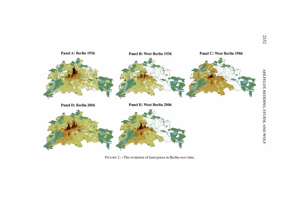
In Figure 2, we display the spatial distribution of land prices across blocksfor each year as a three-dimensional map. The main public parks and forestsare shown in green and the main bodies of water are shown in blue. Whiteareas correspond to other undeveloped areas including railways. Since we usethe same vertical scale for each figure, and land prices are normalized to havea mean of 1 in each year, the levels of the land price surfaces in each figure arecomparable.
As apparent from Panel A of Figure 2, Berlin’s land price gradient in 1936was in fact approximately monocentric, with the highest values concentrated inthe district Mitte. We measure the center of the pre-war Central Business Dis-trict (CBD) as the intersection of Friedrich Strasse and Leipziger Strasse, closeto the underground station City Center (“Stadtmitte”). Around this centralpoint, there are concentric rings of progressively lower land prices surround-ing the pre-war CBD. Towards the Western edge of these concentric rings isthe Kudamm (“Kurfürstendamm”) in Charlottenburg and Wilmersdorf, whichhad developed into a fashionable shopping area in the decades leading up tothe Second World War. This area lies to the West of the Tiergarten Park, whichexplains the gap in land prices between the Kudamm and Mitte. Panel A alsoshows the future line of the Berlin Wall (shown in gray font), including theinner boundary between East and West Berlin and the outer boundary thatseparated West Berlin from its East German hinterland.
To show relative land values in locations that subsequently became part ofWest Berlin, Panel B displays the 1936 distribution of land prices for only theselocations. The two areas of West Berlin with the highest pre-war land prices
2152A
HL
FE
LD
T,RE
DD
ING
,STU
RM
,AN
DW
OL
F
FIGURE 2.—The evolution of land prices in Berlin over time.
THE ECONOMICS OF DENSITY 2153
were parts of a concentric ring around the pre-war CBD: the area around theKudamm discussed above and a second area just west of Potsdamer Platz andthe future line of the Berlin Wall. This second area was a concentration ofcommercial and retail activity surrounding the “Anhalter Bahnhof” mainlineand suburban rail station. Neither of these areas contained substantial gov-ernment administration, which was instead concentrated in Mitte in the futureEast Berlin, particularly around Wilhelmstrasse.
In Panel C, we examine the impact of division by displaying the 1986 distri-bution of land prices for West Berlin. Comparing Panels B and C, three mainfeatures stand out. First, land prices exhibit less dispersion and smaller peakvalues in West Berlin during division than in Berlin during the pre-war pe-riod. Second, one of the pre-war land price peaks in West Berlin—the area justWest of Potsdamer Platz—is entirely eliminated following division, as this areaceased to be an important center of commercial and retail activity. Third, WestBerlin’s CBD during division coincided with the other area of high pre-warland values in West Berlin around the Kudamm, which was relatively centrallylocated within West Berlin.
To examine the impact of reunification, Panel D displays the 2006 distribu-tion of land prices across blocks within Berlin as a whole, while Panel E showsthe same distribution but only for blocks in the former West Berlin. Compar-ing these two figures with the previous two figures, three main features areagain apparent. First, land prices are more dispersed and have higher peakvalues following reunification than during division. Second, the area just Westof Potsdamer Platz is reemerging as a concentration of office and retail devel-opment with high land values. Third, Mitte is also reemerging as a center ofhigh land values. As in the pre-war period, the main government ministries areconcentrated either in Mitte in the former East Berlin or around the federalparliament (“Reichstag”).
Figures A.1 and A.2 in the Technical Data Appendix display the log differ-ence in land prices from 1936 to 1986 and 1986 to 2006 for each block. Asevident from these figures, the largest declines in land prices following divisionand the largest increases in land prices following reunification are along thosesegments of the Berlin Wall around the pre-war CBD. In contrast, there is lit-tle evidence of comparable declines in land prices along other sections of theBerlin Wall. Therefore, these results provide some first evidence that it is notproximity to the Berlin Wall per se that matters, but the loss of access to thepre-war CBD.35
35Regressing the growth in West Berlin floor prices from 1986 to 2006 on their growth from1936 to 1986, we find an estimated coefficient (Conley (1999) standard error) of −0�262 (0.017)and an R2 of 0.29, suggesting that the areas that experienced the largest decline in floor pricesafter division also experienced the largest growth in floor prices after reunification.
2154 AHLFELDT, REDDING, STURM, AND WOLF
5.2. Difference-in-Difference Estimates
To establish the statistical significance of these findings and their robust-ness to the inclusion of controls, we estimate the following “difference-in-difference” specification for division and reunification separately:
� lnOi = α+K∑k=1
Iikβk + lnMiγ+ ui�(22)
where i denotes blocks; � lnOi is the log change in an economic outcome ofinterest (floor prices, workplace employment, residence employment); α is aconstant; Iik is an indicator variable for whether block i lies within a distancegrid cell k from the pre-war CBD; βk are coefficients to be estimated; Mi aretime-invariant observable block characteristics (such as proximity to parks andlakes) and γ captures changes over time in the premium to these time-invariantobservable block characteristics; and ui is a stochastic error. This specificationallows for time-invariant factors that have constant effects over time, which aredifferenced out before and after division (or reunification). It also allows fora common time effect of division or reunification across all blocks, which iscaptured in the constant α.
We begin by considering distance grid cells of 500 meter intervals. Since theminimum distance to the pre-war CBD in West Berlin is around 0.75 kilome-ters, our first distance grid cell is for blocks with distances less than 1.25 kilo-meters. We include grid cells for blocks with distances up to 3.25–3.75 kilome-ters, so that the excluded category is blocks more than 3.75 kilometers fromthe pre-war CBD.36 This grid cells specification allows for a flexible functionalform for the relationship between changes in block economic outcomes anddistance from the pre-war CBD. In these reduced-form regressions, we takethe location of the pre-war CBD as given, whereas in the structural model itslocation is endogenously determined. In Section 5.3, we show that we find sim-ilar results using other nonparametric approaches that do not require us tospecify grid cells, such as locally weighted linear least squares.
We show that our results are robust to two alternative approaches to control-ling for spatial correlation in the error term ui. As our baseline specificationthroughout the paper, we report Heteroscedasticity and Autocorrelation Con-sistent (HAC) standard errors following Conley (1999), which allow for spatialcorrelation in the errors across neighboring blocks with distances less than aspecified threshold.37 As a robustness check, the Technical Data Appendix re-ports standard errors clustered on statistical areas (“Gebiete”), which allows
36The numbers of West Berlin blocks with floor price data in all three years in each grid cell(from nearest to furthest from the pre-war CBD) are: 23, 37, 50, 84, 146, and 173. The maximumdistance to the pre-war CBD in West Berlin is around 23 kilometers.
37We use a threshold of 0.5 kilometers, where the median block in Berlin has 19 other blockswithin 0.5 kilometers.
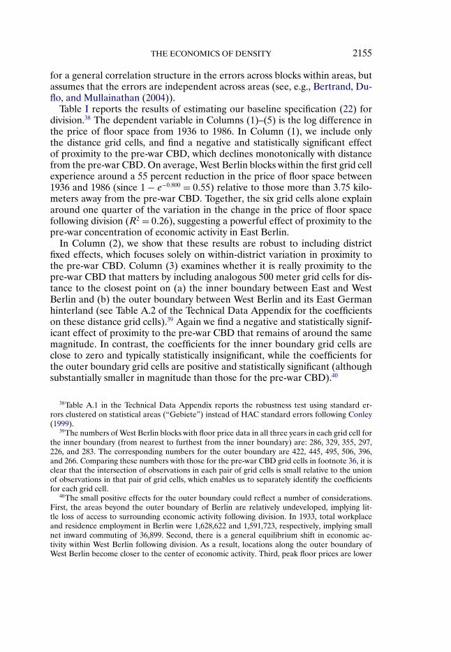
THE ECONOMICS OF DENSITY 2155
for a general correlation structure in the errors across blocks within areas, butassumes that the errors are independent across areas (see, e.g., Bertrand, Du-flo, and Mullainathan (2004)).
Table I reports the results of estimating our baseline specification (22) fordivision.38 The dependent variable in Columns (1)–(5) is the log difference inthe price of floor space from 1936 to 1986. In Column (1), we include onlythe distance grid cells, and find a negative and statistically significant effectof proximity to the pre-war CBD, which declines monotonically with distancefrom the pre-war CBD. On average, West Berlin blocks within the first grid cellexperience around a 55 percent reduction in the price of floor space between1936 and 1986 (since 1 − e−0�800 = 0�55) relative to those more than 3.75 kilo-meters away from the pre-war CBD. Together, the six grid cells alone explainaround one quarter of the variation in the change in the price of floor spacefollowing division (R2 = 0�26), suggesting a powerful effect of proximity to thepre-war concentration of economic activity in East Berlin.
In Column (2), we show that these results are robust to including districtfixed effects, which focuses solely on within-district variation in proximity tothe pre-war CBD. Column (3) examines whether it is really proximity to thepre-war CBD that matters by including analogous 500 meter grid cells for dis-tance to the closest point on (a) the inner boundary between East and WestBerlin and (b) the outer boundary between West Berlin and its East Germanhinterland (see Table A.2 of the Technical Data Appendix for the coefficientson these distance grid cells).39 Again we find a negative and statistically signif-icant effect of proximity to the pre-war CBD that remains of around the samemagnitude. In contrast, the coefficients for the inner boundary grid cells areclose to zero and typically statistically insignificant, while the coefficients forthe outer boundary grid cells are positive and statistically significant (althoughsubstantially smaller in magnitude than those for the pre-war CBD).40
38Table A.1 in the Technical Data Appendix reports the robustness test using standard er-rors clustered on statistical areas (“Gebiete”) instead of HAC standard errors following Conley(1999).
39The numbers of West Berlin blocks with floor price data in all three years in each grid cell forthe inner boundary (from nearest to furthest from the inner boundary) are: 286, 329, 355, 297,226, and 283. The corresponding numbers for the outer boundary are 422, 445, 495, 506, 396,and 266. Comparing these numbers with those for the pre-war CBD grid cells in footnote 36, it isclear that the intersection of observations in each pair of grid cells is small relative to the unionof observations in that pair of grid cells, which enables us to separately identify the coefficientsfor each grid cell.
40The small positive effects for the outer boundary could reflect a number of considerations.First, the areas beyond the outer boundary of Berlin are relatively undeveloped, implying lit-tle loss of access to surrounding economic activity following division. In 1933, total workplaceand residence employment in Berlin were 1,628,622 and 1,591,723, respectively, implying smallnet inward commuting of 36,899. Second, there is a general equilibrium shift in economic ac-tivity within West Berlin following division. As a result, locations along the outer boundary ofWest Berlin become closer to the center of economic activity. Third, peak floor prices are lower
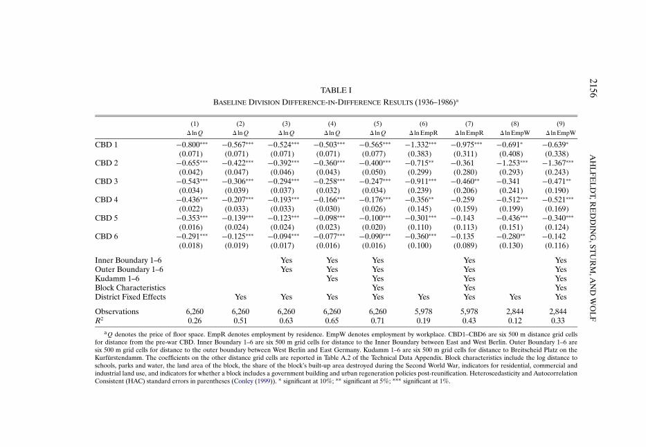
2156A
HL
FE
LD
T,RE
DD
ING
,STU
RM
,AN
DW
OL
F
TABLE I
BASELINE DIVISION DIFFERENCE-IN-DIFFERENCE RESULTS (1936–1986)a
(1) (2) (3) (4) (5) (6) (7) (8) (9)� lnQ � lnQ � lnQ � lnQ � lnQ � ln EmpR � ln EmpR � ln EmpW � ln EmpW
CBD 1 −0�800∗∗∗ −0�567∗∗∗ −0�524∗∗∗ −0�503∗∗∗ −0�565∗∗∗ −1�332∗∗∗ −0�975∗∗∗ −0�691∗ −0�639∗
(0�071) (0�071) (0�071) (0�071) (0�077) (0�383) (0�311) (0�408) (0�338)CBD 2 −0�655∗∗∗ −0�422∗∗∗ −0�392∗∗∗ −0�360∗∗∗ −0�400∗∗∗ −0�715∗∗ −0�361 −1�253∗∗∗ −1�367∗∗∗
(0�042) (0�047) (0�046) (0�043) (0�050) (0�299) (0�280) (0�293) (0�243)CBD 3 −0�543∗∗∗ −0�306∗∗∗ −0�294∗∗∗ −0�258∗∗∗ −0�247∗∗∗ −0�911∗∗∗ −0�460∗∗ −0�341 −0�471∗∗
(0�034) (0�039) (0�037) (0�032) (0�034) (0�239) (0�206) (0�241) (0�190)CBD 4 −0�436∗∗∗ −0�207∗∗∗ −0�193∗∗∗ −0�166∗∗∗ −0�176∗∗∗ −0�356∗∗ −0�259 −0�512∗∗∗ −0�521∗∗∗
(0�022) (0�033) (0�033) (0�030) (0�026) (0�145) (0�159) (0�199) (0�169)CBD 5 −0�353∗∗∗ −0�139∗∗∗ −0�123∗∗∗ −0�098∗∗∗ −0�100∗∗∗ −0�301∗∗∗ −0�143 −0�436∗∗∗ −0�340∗∗∗
(0�016) (0�024) (0�024) (0�023) (0�020) (0�110) (0�113) (0�151) (0�124)CBD 6 −0�291∗∗∗ −0�125∗∗∗ −0�094∗∗∗ −0�077∗∗∗ −0�090∗∗∗ −0�360∗∗∗ −0�135 −0�280∗∗ −0�142
(0�018) (0�019) (0�017) (0�016) (0�016) (0�100) (0�089) (0�130) (0�116)
Inner Boundary 1–6 Yes Yes Yes Yes YesOuter Boundary 1–6 Yes Yes Yes Yes YesKudamm 1–6 Yes Yes Yes YesBlock Characteristics Yes Yes YesDistrict Fixed Effects Yes Yes Yes Yes Yes Yes Yes Yes
Observations 6,260 6,260 6,260 6,260 6,260 5,978 5,978 2,844 2,844R2 0.26 0.51 0.63 0.65 0.71 0.19 0.43 0.12 0.33
aQ denotes the price of floor space. EmpR denotes employment by residence. EmpW denotes employment by workplace. CBD1–CBD6 are six 500 m distance grid cellsfor distance from the pre-war CBD. Inner Boundary 1–6 are six 500 m grid cells for distance to the Inner Boundary between East and West Berlin. Outer Boundary 1–6 aresix 500 m grid cells for distance to the outer boundary between West Berlin and East Germany. Kudamm 1–6 are six 500 m grid cells for distance to Breitscheid Platz on theKurfürstendamm. The coefficients on the other distance grid cells are reported in Table A.2 of the Technical Data Appendix. Block characteristics include the log distance toschools, parks and water, the land area of the block, the share of the block’s built-up area destroyed during the Second World War, indicators for residential, commercial andindustrial land use, and indicators for whether a block includes a government building and urban regeneration policies post-reunification. Heteroscedasticity and AutocorrelationConsistent (HAC) standard errors in parentheses (Conley (1999)). ∗ significant at 10%; ∗∗ significant at 5%; ∗∗∗ significant at 1%.
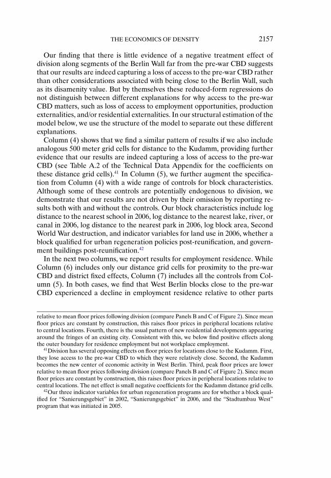
THE ECONOMICS OF DENSITY 2157
Our finding that there is little evidence of a negative treatment effect ofdivision along segments of the Berlin Wall far from the pre-war CBD suggeststhat our results are indeed capturing a loss of access to the pre-war CBD ratherthan other considerations associated with being close to the Berlin Wall, suchas its disamenity value. But by themselves these reduced-form regressions donot distinguish between different explanations for why access to the pre-warCBD matters, such as loss of access to employment opportunities, productionexternalities, and/or residential externalities. In our structural estimation of themodel below, we use the structure of the model to separate out these differentexplanations.
Column (4) shows that we find a similar pattern of results if we also includeanalogous 500 meter grid cells for distance to the Kudamm, providing furtherevidence that our results are indeed capturing a loss of access to the pre-warCBD (see Table A.2 of the Technical Data Appendix for the coefficients onthese distance grid cells).41 In Column (5), we further augment the specifica-tion from Column (4) with a wide range of controls for block characteristics.Although some of these controls are potentially endogenous to division, wedemonstrate that our results are not driven by their omission by reporting re-sults both with and without the controls. Our block characteristics include logdistance to the nearest school in 2006, log distance to the nearest lake, river, orcanal in 2006, log distance to the nearest park in 2006, log block area, SecondWorld War destruction, and indicator variables for land use in 2006, whether ablock qualified for urban regeneration policies post-reunification, and govern-ment buildings post-reunification.42
In the next two columns, we report results for employment residence. WhileColumn (6) includes only our distance grid cells for proximity to the pre-warCBD and district fixed effects, Column (7) includes all the controls from Col-umn (5). In both cases, we find that West Berlin blocks close to the pre-warCBD experienced a decline in employment residence relative to other parts
relative to mean floor prices following division (compare Panels B and C of Figure 2). Since meanfloor prices are constant by construction, this raises floor prices in peripheral locations relativeto central locations. Fourth, there is the usual pattern of new residential developments appearingaround the fringes of an existing city. Consistent with this, we below find positive effects alongthe outer boundary for residence employment but not workplace employment.
41Division has several opposing effects on floor prices for locations close to the Kudamm. First,they lose access to the pre-war CBD to which they were relatively close. Second, the Kudammbecomes the new center of economic activity in West Berlin. Third, peak floor prices are lowerrelative to mean floor prices following division (compare Panels B and C of Figure 2). Since meanfloor prices are constant by construction, this raises floor prices in peripheral locations relative tocentral locations. The net effect is small negative coefficients for the Kudamm distance grid cells.
42Our three indicator variables for urban regeneration programs are for whether a block qual-ified for “Sanierungsgebiet” in 2002, “Sanierungsgebiet” in 2006, and the “Stadtumbau West”program that was initiated in 2005.
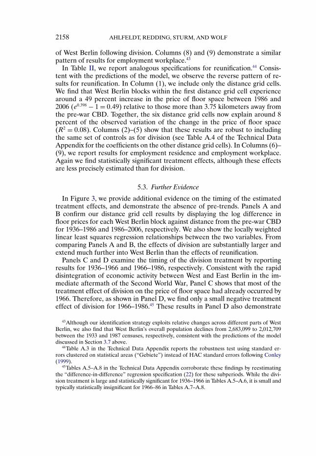
2158 AHLFELDT, REDDING, STURM, AND WOLF
of West Berlin following division. Columns (8) and (9) demonstrate a similarpattern of results for employment workplace.43
In Table II, we report analogous specifications for reunification.44 Consis-tent with the predictions of the model, we observe the reverse pattern of re-sults for reunification. In Column (1), we include only the distance grid cells.We find that West Berlin blocks within the first distance grid cell experiencearound a 49 percent increase in the price of floor space between 1986 and2006 (e0�398 − 1 = 0�49) relative to those more than 3.75 kilometers away fromthe pre-war CBD. Together, the six distance grid cells now explain around 8percent of the observed variation of the change in the price of floor space(R2 = 0�08). Columns (2)–(5) show that these results are robust to includingthe same set of controls as for division (see Table A.4 of the Technical DataAppendix for the coefficients on the other distance grid cells). In Columns (6)–(9), we report results for employment residence and employment workplace.Again we find statistically significant treatment effects, although these effectsare less precisely estimated than for division.
5.3. Further Evidence
In Figure 3, we provide additional evidence on the timing of the estimatedtreatment effects, and demonstrate the absence of pre-trends. Panels A andB confirm our distance grid cell results by displaying the log difference infloor prices for each West Berlin block against distance from the pre-war CBDfor 1936–1986 and 1986–2006, respectively. We also show the locally weightedlinear least squares regression relationships between the two variables. Fromcomparing Panels A and B, the effects of division are substantially larger andextend much further into West Berlin than the effects of reunification.
Panels C and D examine the timing of the division treatment by reportingresults for 1936–1966 and 1966–1986, respectively. Consistent with the rapiddisintegration of economic activity between West and East Berlin in the im-mediate aftermath of the Second World War, Panel C shows that most of thetreatment effect of division on the price of floor space had already occurred by1966. Therefore, as shown in Panel D, we find only a small negative treatmenteffect of division for 1966–1986.45 These results in Panel D also demonstrate
43Although our identification strategy exploits relative changes across different parts of WestBerlin, we also find that West Berlin’s overall population declines from 2,683,099 to 2,012,709between the 1933 and 1987 censuses, respectively, consistent with the predictions of the modeldiscussed in Section 3.7 above.
44Table A.3 in the Technical Data Appendix reports the robustness test using standard er-rors clustered on statistical areas (“Gebiete”) instead of HAC standard errors following Conley(1999).
45Tables A.5–A.8 in the Technical Data Appendix corroborate these findings by reestimatingthe “difference-in-difference” regression specification (22) for these subperiods. While the divi-sion treatment is large and statistically significant for 1936–1966 in Tables A.5–A.6, it is small andtypically statistically insignificant for 1966–86 in Tables A.7–A.8.
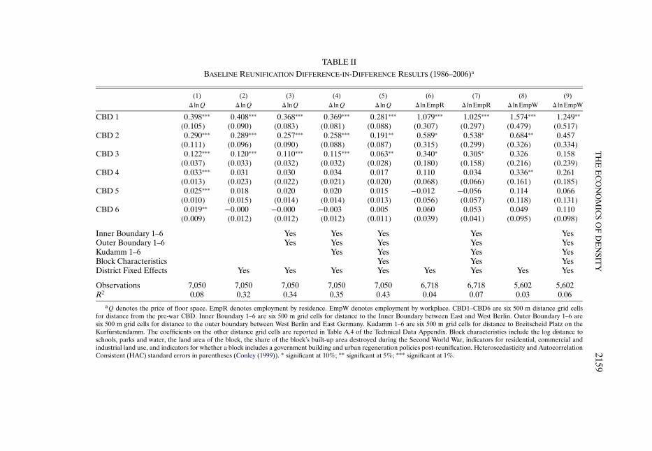
TH
EE
CO
NO
MIC
SO
FD
EN
SITY
2159TABLE II
BASELINE REUNIFICATION DIFFERENCE-IN-DIFFERENCE RESULTS (1986–2006)a
(1) (2) (3) (4) (5) (6) (7) (8) (9)� lnQ � lnQ � lnQ � lnQ � lnQ � ln EmpR � ln EmpR � ln EmpW � ln EmpW
CBD 1 0�398∗∗∗ 0�408∗∗∗ 0�368∗∗∗ 0�369∗∗∗ 0�281∗∗∗ 1�079∗∗∗ 1�025∗∗∗ 1�574∗∗∗ 1�249∗∗
(0�105) (0�090) (0�083) (0�081) (0�088) (0�307) (0�297) (0�479) (0�517)CBD 2 0�290∗∗∗ 0�289∗∗∗ 0�257∗∗∗ 0�258∗∗∗ 0�191∗∗ 0�589∗ 0�538∗ 0�684∗∗ 0�457
(0�111) (0�096) (0�090) (0�088) (0�087) (0�315) (0�299) (0�326) (0�334)CBD 3 0�122∗∗∗ 0�120∗∗∗ 0�110∗∗∗ 0�115∗∗∗ 0�063∗∗ 0�340∗ 0�305∗ 0�326 0�158
(0�037) (0�033) (0�032) (0�032) (0�028) (0�180) (0�158) (0�216) (0�239)CBD 4 0�033∗∗∗ 0�031 0�030 0�034 0�017 0�110 0�034 0�336∗∗ 0�261
(0�013) (0�023) (0�022) (0�021) (0�020) (0�068) (0�066) (0�161) (0�185)CBD 5 0�025∗∗∗ 0�018 0�020 0�020 0�015 −0�012 −0�056 0�114 0�066
(0�010) (0�015) (0�014) (0�014) (0�013) (0�056) (0�057) (0�118) (0�131)CBD 6 0�019∗∗ −0�000 −0�000 −0�003 0�005 0�060 0�053 0�049 0�110
(0�009) (0�012) (0�012) (0�012) (0�011) (0�039) (0�041) (0�095) (0�098)
Inner Boundary 1–6 Yes Yes Yes Yes YesOuter Boundary 1–6 Yes Yes Yes Yes YesKudamm 1–6 Yes Yes Yes YesBlock Characteristics Yes Yes YesDistrict Fixed Effects Yes Yes Yes Yes Yes Yes Yes Yes
Observations 7,050 7,050 7,050 7,050 7,050 6,718 6,718 5,602 5,602R2 0.08 0.32 0.34 0.35 0.43 0.04 0.07 0.03 0.06
aQ denotes the price of floor space. EmpR denotes employment by residence. EmpW denotes employment by workplace. CBD1–CBD6 are six 500 m distance grid cellsfor distance from the pre-war CBD. Inner Boundary 1–6 are six 500 m grid cells for distance to the Inner Boundary between East and West Berlin. Outer Boundary 1–6 aresix 500 m grid cells for distance to the outer boundary between West Berlin and East Germany. Kudamm 1–6 are six 500 m grid cells for distance to Breitscheid Platz on theKurfürstendamm. The coefficients on the other distance grid cells are reported in Table A.4 of the Technical Data Appendix. Block characteristics include the log distance toschools, parks and water, the land area of the block, the share of the block’s built-up area destroyed during the Second World War, indicators for residential, commercial andindustrial land use, and indicators for whether a block includes a government building and urban regeneration policies post-reunification. Heteroscedasticity and AutocorrelationConsistent (HAC) standard errors in parentheses (Conley (1999)). ∗ significant at 10%; ∗∗ significant at 5%; ∗∗∗ significant at 1%.
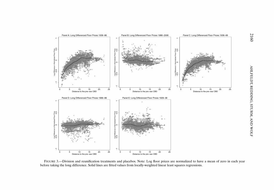
2160A
HL
FE
LD
T,RE
DD
ING
,STU
RM
,AN
DW
OL
F
FIGURE 3.—Division and reunification treatments and placebos. Note: Log floor prices are normalized to have a mean of zero in each yearbefore taking the long difference. Solid lines are fitted values from locally-weighted linear least squares regressions.
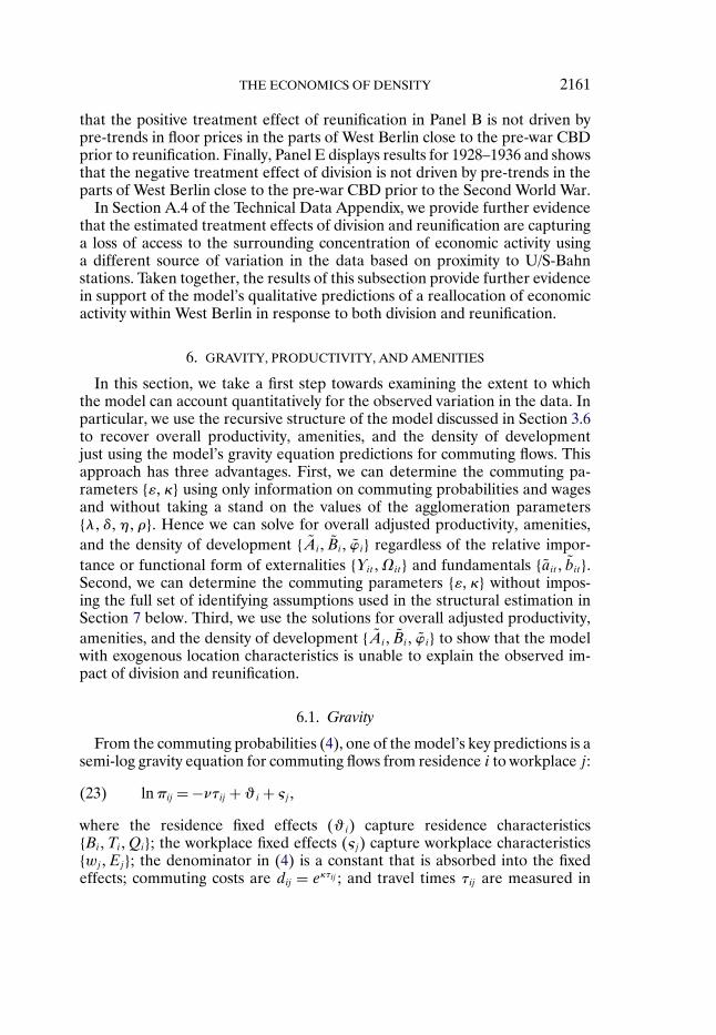
THE ECONOMICS OF DENSITY 2161
that the positive treatment effect of reunification in Panel B is not driven bypre-trends in floor prices in the parts of West Berlin close to the pre-war CBDprior to reunification. Finally, Panel E displays results for 1928–1936 and showsthat the negative treatment effect of division is not driven by pre-trends in theparts of West Berlin close to the pre-war CBD prior to the Second World War.
In Section A.4 of the Technical Data Appendix, we provide further evidencethat the estimated treatment effects of division and reunification are capturinga loss of access to the surrounding concentration of economic activity usinga different source of variation in the data based on proximity to U/S-Bahnstations. Taken together, the results of this subsection provide further evidencein support of the model’s qualitative predictions of a reallocation of economicactivity within West Berlin in response to both division and reunification.
6. GRAVITY, PRODUCTIVITY, AND AMENITIES
In this section, we take a first step towards examining the extent to whichthe model can account quantitatively for the observed variation in the data. Inparticular, we use the recursive structure of the model discussed in Section 3.6to recover overall productivity, amenities, and the density of developmentjust using the model’s gravity equation predictions for commuting flows. Thisapproach has three advantages. First, we can determine the commuting pa-rameters {ε�κ} using only information on commuting probabilities and wagesand without taking a stand on the values of the agglomeration parameters{λ�δ�η�ρ}. Hence we can solve for overall adjusted productivity, amenities,and the density of development {Ai� Bi� ϕi} regardless of the relative impor-tance or functional form of externalities {Υit�Ωit} and fundamentals {ait� bit}.Second, we can determine the commuting parameters {ε�κ} without impos-ing the full set of identifying assumptions used in the structural estimation inSection 7 below. Third, we use the solutions for overall adjusted productivity,amenities, and the density of development {Ai� Bi� ϕi} to show that the modelwith exogenous location characteristics is unable to explain the observed im-pact of division and reunification.
6.1. Gravity
From the commuting probabilities (4), one of the model’s key predictions is asemi-log gravity equation for commuting flows from residence i to workplace j:
lnπij = −ντij +ϑi + ςj�(23)
where the residence fixed effects (ϑi) capture residence characteristics{Bi�Ti�Qi}; the workplace fixed effects (ςj) capture workplace characteristics{wj�Ej}; the denominator in (4) is a constant that is absorbed into the fixedeffects; commuting costs are dij = eκτij ; and travel times τij are measured in
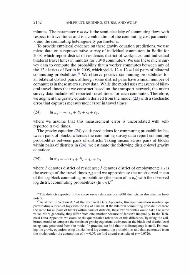
2162 AHLFELDT, REDDING, STURM, AND WOLF
minutes. The parameter ν = εκ is the semi-elasticity of commuting flows withrespect to travel times and is a combination of the commuting cost parameterκ and the commuting heterogeneity parameter ε.
To provide empirical evidence on these gravity equation predictions, we usemicro data on a representative survey of individual commuters in Berlin for2008, which report district of residence, district of workplace, and individualbilateral travel times in minutes for 7,948 commuters. We use these micro sur-vey data to compute the probability that a worker commutes between any ofthe 12 districts of Berlin in 2008, which yields 12 × 12 = 144 pairs of bilateralcommuting probabilities.46 We observe positive commuting probabilities forall bilateral district pairs, although some district pairs have a small number ofcommuters in these micro survey data. While the model uses measures of bilat-eral travel times that we construct based on the transport network, the microsurvey data include self-reported travel times for each commuter. Therefore,we augment the gravity equation derived from the model (23) with a stochasticerror that captures measurement error in travel times:
lnπij = −ντij +ϑi + ςj + eij�(24)
where we assume that this measurement error is uncorrelated with self-reported travel times.
The gravity equation (24) yields predictions for commuting probabilities be-tween pairs of blocks, whereas the commuting survey data report commutingprobabilities between pairs of districts. Taking means across pairs of blockswithin pairs of districts in (24), we estimate the following district-level gravityequation:
lnπIJ = −ντIJ +ϑI + ςJ + eIJ�(25)
where I denotes district of residence; J denotes district of employment; τIJ isthe average of the travel times τij ; and we approximate the unobserved meanof the log block commuting probabilities (the mean of lnπij) with the observedlog district commuting probabilities (lnπIJ).47
46The districts reported in the micro survey data are post-2001 districts, as discussed in foot-note 9.
47As shown in Section A.2 of the Technical Data Appendix, this approximation involves ap-proximating a mean of logs with the log of a mean. If the bilateral commuting probabilities werethe same for all pairs of blocks within pairs of districts, these two variables would take the samevalue. More generally, they differ from one another because of Jensen’s inequality. In the Tech-nical Data Appendix, we examine the quantitative relevance of this difference, by using the cali-brated model to compare the results of gravity equations estimated at the block and district levelusing data generated from the model. In practice, we find that this discrepancy is small. Estimat-ing the gravity equation using district-level log commuting probabilities and data generated fromthe model under the assumption of ν = 0�07, we find a semi-elasticity of ν = 0�0726.
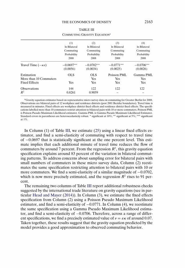
THE ECONOMICS OF DENSITY 2163
TABLE III
COMMUTING GRAVITY EQUATIONa
(1) (2) (3) (4)ln Bilateral ln Bilateral ln Bilateral ln BilateralCommuting Commuting Commuting CommutingProbability Probability Probability Probability
2008 2008 2008 2008
Travel Time (−κε) −0�0697∗∗∗ −0�0702∗∗∗ −0�0771∗∗∗ −0�0706∗∗∗
(0�0056) (0�0034) (0�0025) (0�0026)
Estimation OLS OLS Poisson PML Gamma PMLMore than 10 Commuters Yes Yes YesFixed Effects Yes Yes Yes Yes
Observations 144 122 122 122R2 0.8261 0.9059 – –
aGravity equation estimates based on representative micro survey data on commuting for Greater Berlin for 2008.Observations are bilateral pairs of 12 workplace and residence districts (post 2001 Bezirke boundaries). Travel time ismeasured in minutes. Fixed effects are workplace district fixed effects and residence district fixed effects. The specifi-cations labelled more than 10 commuters restrict attention to bilateral pairs with 10 or more commuters. Poisson PMLis Poisson Pseudo Maximum Likelihood estimator. Gamma PML is Gamma Pseudo Maximum Likelihood Estimator.Standard errors in parentheses are heteroscedasticity robust. ∗ significant at 10%; ∗∗ significant at 5%; ∗∗∗ significantat 1%.
In Column (1) of Table III, we estimate (25) using a linear fixed effects es-timator, and find a semi-elasticity of commuting with respect to travel timeof −0�0697 that is statistically significant at the one percent level. This esti-mate implies that each additional minute of travel time reduces the flow ofcommuters by around 7 percent. From the regression R2, this gravity equationspecification explains around 83 percent of the variation in bilateral commut-ing patterns. To address concerns about sampling error for bilateral pairs withsmall numbers of commuters in these micro survey data, Column (2) reesti-mates the same specification restricting attention to bilateral pairs with 10 ormore commuters. We find a semi-elasticity of a similar magnitude of −0�0702,which is now more precisely estimated, and the regression R2 rises to 91 per-cent.
The remaining two columns of Table III report additional robustness checkssuggested by the international trade literature on gravity equations (see in par-ticular Head and Mayer (2014)). In Column (3), we estimate the fixed effectsspecification from Column (2) using a Poisson Pseudo Maximum Likelihoodestimator, and find a semi-elasticity of −0�0771. In Column (4), we reestimatethe same specification using a Gamma Pseudo Maximum Likelihood estima-tor, and find a semi-elasticity of −0�0706. Therefore, across a range of differ-ent specifications, we find a precisely estimated value of ν = εκ of around 0�07.Taken together, these results suggest that the gravity equation predicted by themodel provides a good approximation to observed commuting behavior.
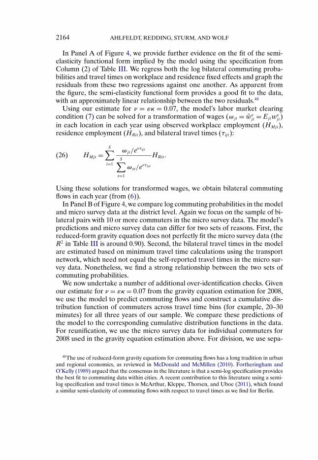
2164 AHLFELDT, REDDING, STURM, AND WOLF
In Panel A of Figure 4, we provide further evidence on the fit of the semi-elasticity functional form implied by the model using the specification fromColumn (2) of Table III. We regress both the log bilateral commuting proba-bilities and travel times on workplace and residence fixed effects and graph theresiduals from these two regressions against one another. As apparent fromthe figure, the semi-elasticity functional form provides a good fit to the data,with an approximately linear relationship between the two residuals.48
Using our estimate for ν = εκ = 0�07, the model’s labor market clearingcondition (7) can be solved for a transformation of wages (ωjt = wε
jt = Ejtwεjt)
in each location in each year using observed workplace employment (HMjt),residence employment (HRit), and bilateral travel times (τijt):
HMjt =S∑i=1
ωjt/eντijt
S∑s=1
ωst/eντist
HRit �(26)
Using these solutions for transformed wages, we obtain bilateral commutingflows in each year (from (6)).
In Panel B of Figure 4, we compare log commuting probabilities in the modeland micro survey data at the district level. Again we focus on the sample of bi-lateral pairs with 10 or more commuters in the micro survey data. The model’spredictions and micro survey data can differ for two sets of reasons. First, thereduced-form gravity equation does not perfectly fit the micro survey data (theR2 in Table III is around 0.90). Second, the bilateral travel times in the modelare estimated based on minimum travel time calculations using the transportnetwork, which need not equal the self-reported travel times in the micro sur-vey data. Nonetheless, we find a strong relationship between the two sets ofcommuting probabilities.
We now undertake a number of additional over-identification checks. Givenour estimate for ν = εκ= 0�07 from the gravity equation estimation for 2008,we use the model to predict commuting flows and construct a cumulative dis-tribution function of commuters across travel time bins (for example, 20–30minutes) for all three years of our sample. We compare these predictions ofthe model to the corresponding cumulative distribution functions in the data.For reunification, we use the micro survey data for individual commuters for2008 used in the gravity equation estimation above. For division, we use sepa-
48The use of reduced-form gravity equations for commuting flows has a long tradition in urbanand regional economics, as reviewed in McDonald and McMillen (2010). Fortheringham andO’Kelly (1989) argued that the consensus in the literature is that a semi-log specification providesthe best fit to commuting data within cities. A recent contribution to this literature using a semi-log specification and travel times is McArthur, Kleppe, Thorsen, and Uboe (2011), which founda similar semi-elasticity of commuting flows with respect to travel times as we find for Berlin.
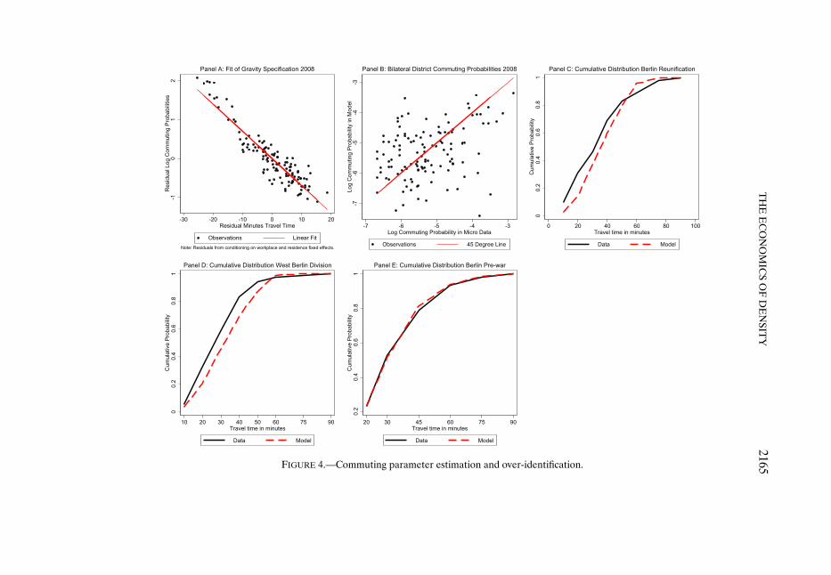
TH
EE
CO
NO
MIC
SO
FD
EN
SITY
2165FIGURE 4.—Commuting parameter estimation and over-identification.
2166 AHLFELDT, REDDING, STURM, AND WOLF
rate data on the fractions of workers in discrete travel time bins from a repre-sentative sample of commuters in West Berlin in 1982. For the pre-war period,we use the data reported in Feder (1939).
In Panel C of Figure 4, we show the cumulative distribution functions of com-muters across the travel time bins in the model and micro survey data for Berlinin 2008. Although these moments were not used in the gravity equation esti-mation of ν = εκ above, we find that the model approximates the cumulativedistribution function in the data well. In Panel D of Figure 4, we undertake thesame exercise for West Berlin in 1986. Although the smaller geographic areaof West Berlin ensures that it has a quite different distribution of workplaceemployment, residence employment, and travel times from Berlin as a whole,we again find that the model approximates the relationship in the data. Finally,in Panel E of Figure 4, we repeat the exercise for Berlin in 1936. Although thedistribution of travel times for Berlin differs between 1936 (based on publictransport) and 2006 (based on public transport and private automobiles), weagain find that the model has explanatory power for the data.49
Therefore, despite our model necessarily being an abstraction, we find thatit is successful in capturing the key features of commuting patterns in Berlinduring our sample period, and successfully predicts moments not used in theestimation of the commuting parameters.
6.2. Productivity and Amenities
We now use the gravity equation estimation to recover overall adjusted pro-ductivity, amenities, and the density of development {Ait� Bit� ϕi}. We use themodel to recover these objects without taking a stand of the relative impor-tance of externalities and fundamentals. From profit maximization and zeroprofits (12), log adjusted final goods productivity relative to its geometric meanis
ln(Ait
At
)= (1 − α) ln
(Qit
Qt
)+ α
εln
(ωit
ωt
)�(27)
where a bar above a variable again denotes a geometric mean, so that At =exp{ 1
S
∑S
s=1 ln Ast}. Intuitively, high floor prices and wages in (27) require highfinal goods productivity in order for zero profits to be satisfied.
49Consistent with the results in Duranton and Turner (2011) for U.S. metropolitan areas, wefind that the majority of commuters in Berlin have travel times of less than forty-five minutes inall three years of our sample.
THE ECONOMICS OF DENSITY 2167
From the residential choice probabilities (5) and population mobility withthe larger economy (9), log residential amenities relative to their geometricmean are
ln(Bit
Bt
)= 1ε
ln(HRit
HRt
)+ (1 −β) ln
(Qit
Qt
)− 1ε
ln(Wit
W t
)�(28)
whereWit is a measure of commuting market access that can be written in termsof the transformed wages (ωit) from the commuting market clearing condition(26):
Wit =S∑s=1
ωst/eντist � ωst = wε
st =Estwεst �(29)
Intuitively, high residence employment and high floor prices in (28) must beexplained either by high commuting market access or by attractive residentialamenities. Using residential land market clearing (17) and commercial landmarket clearing (18), we can also recover the adjusted density of developmentrelative to its geometric mean.
To solve for adjusted productivity, amenities, and the density of develop-ment, we require values for a subset of the model’s parameters: {α�β�μ�ε�κ}.Of these parameters, the share of residential floor space in consumer expen-diture (1 − β), the share of commercial floor space in firm costs (1 − α), andthe share of land in construction costs (1 −μ) are hard to determine from ourdata, because information on consumer expenditures and factor payments atthe block level is not available over our long historical sample period. As thereis a degree of consensus about the values of these parameters, we set themequal to central estimates from the existing empirical literature. We set theshare of consumer expenditure on residential floor space (1 −β) equal to 0.25,which is consistent with the estimates in Davis and Ortalo-Magné (2011). Weassume that the share of firm expenditure on commercial floor space (1 − α)is 0.20, which is in line with the findings of Valentinyi and Herrendorf (2008).We set the share of land in construction costs (1 − μ) equal to 0.25, whichis consistent with the values in Combes, Duranton, and Gobillon (2014) andEpple, Gordon, and Sieg (2010) and with micro data on property transactionsthat is available for Berlin from 2000 to 2012, as discussed in the SupplementalMaterial.
We use our estimate of ν = εκ= 0�07 from the gravity equation estimationabove. To calibrate the value of the Fréchet shape parameter (ε), we use ourdata on the dispersion of log wages by workplace across the districts of WestBerlin for 1986. From the labor market clearing condition (26), transformedwages (ωit) are determined independently of ε from workplace employment,residence employment, and travel times. Therefore, ε merely determines themonotonic transformation that maps transformed wages (ωit) into adjusted
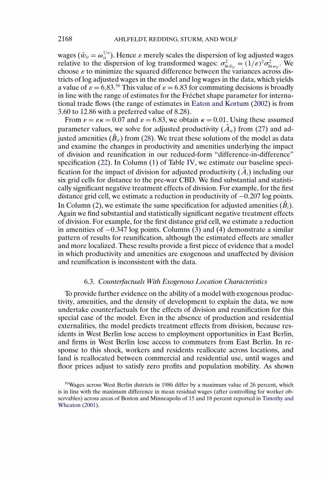
2168 AHLFELDT, REDDING, STURM, AND WOLF
wages (wit =ω1/εit ). Hence ε merely scales the dispersion of log adjusted wages
relative to the dispersion of log transformed wages: σ2ln wit
= (1/ε)2σ2lnωit
. Wechoose ε to minimize the squared difference between the variances across dis-tricts of log adjusted wages in the model and log wages in the data, which yieldsa value of ε= 6�83.50 This value of ε= 6�83 for commuting decisions is broadlyin line with the range of estimates for the Fréchet shape parameter for interna-tional trade flows (the range of estimates in Eaton and Kortum (2002) is from3.60 to 12.86 with a preferred value of 8.28).
From ν = εκ= 0�07 and ε= 6�83, we obtain κ= 0�01. Using these assumedparameter values, we solve for adjusted productivity (Ait) from (27) and ad-justed amenities (Bit) from (28). We treat these solutions of the model as dataand examine the changes in productivity and amenities underlying the impactof division and reunification in our reduced-form “difference-in-difference”specification (22). In Column (1) of Table IV, we estimate our baseline speci-fication for the impact of division for adjusted productivity (Ai) including oursix grid cells for distance to the pre-war CBD. We find substantial and statisti-cally significant negative treatment effects of division. For example, for the firstdistance grid cell, we estimate a reduction in productivity of −0�207 log points.In Column (2), we estimate the same specification for adjusted amenities (Bi).Again we find substantial and statistically significant negative treatment effectsof division. For example, for the first distance grid cell, we estimate a reductionin amenities of −0�347 log points. Columns (3) and (4) demonstrate a similarpattern of results for reunification, although the estimated effects are smallerand more localized. These results provide a first piece of evidence that a modelin which productivity and amenities are exogenous and unaffected by divisionand reunification is inconsistent with the data.
6.3. Counterfactuals With Exogenous Location Characteristics
To provide further evidence on the ability of a model with exogenous produc-tivity, amenities, and the density of development to explain the data, we nowundertake counterfactuals for the effects of division and reunification for thisspecial case of the model. Even in the absence of production and residentialexternalities, the model predicts treatment effects from division, because res-idents in West Berlin lose access to employment opportunities in East Berlin,and firms in West Berlin lose access to commuters from East Berlin. In re-sponse to this shock, workers and residents reallocate across locations, andland is reallocated between commercial and residential use, until wages andfloor prices adjust to satisfy zero profits and population mobility. As shown
50Wages across West Berlin districts in 1986 differ by a maximum value of 26 percent, whichis in line with the maximum difference in mean residual wages (after controlling for worker ob-servables) across areas of Boston and Minneapolis of 15 and 18 percent reported in Timothy andWheaton (2001).
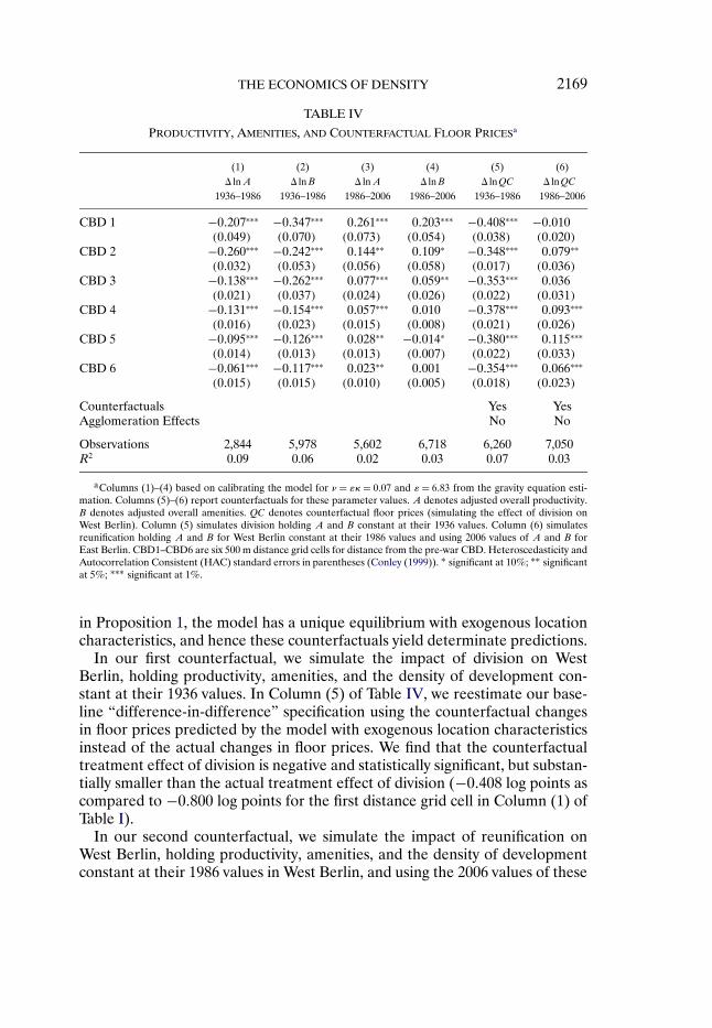
THE ECONOMICS OF DENSITY 2169
TABLE IV
PRODUCTIVITY, AMENITIES, AND COUNTERFACTUAL FLOOR PRICESa
(1) (2) (3) (4) (5) (6)� lnA � lnB � lnA � lnB � ln QC � ln QC
1936–1986 1936–1986 1986–2006 1986–2006 1936–1986 1986–2006
CBD 1 −0�207∗∗∗ −0�347∗∗∗ 0�261∗∗∗ 0�203∗∗∗ −0�408∗∗∗ −0�010(0�049) (0�070) (0�073) (0�054) (0�038) (0�020)
CBD 2 −0�260∗∗∗ −0�242∗∗∗ 0�144∗∗ 0�109∗ −0�348∗∗∗ 0�079∗∗
(0�032) (0�053) (0�056) (0�058) (0�017) (0�036)CBD 3 −0�138∗∗∗ −0�262∗∗∗ 0�077∗∗∗ 0�059∗∗ −0�353∗∗∗ 0�036
(0�021) (0�037) (0�024) (0�026) (0�022) (0�031)CBD 4 −0�131∗∗∗ −0�154∗∗∗ 0�057∗∗∗ 0�010 −0�378∗∗∗ 0�093∗∗∗
(0�016) (0�023) (0�015) (0�008) (0�021) (0�026)CBD 5 −0�095∗∗∗ −0�126∗∗∗ 0�028∗∗ −0�014∗ −0�380∗∗∗ 0�115∗∗∗
(0�014) (0�013) (0�013) (0�007) (0�022) (0�033)CBD 6 −0�061∗∗∗ −0�117∗∗∗ 0�023∗∗ 0�001 −0�354∗∗∗ 0�066∗∗∗
(0�015) (0�015) (0�010) (0�005) (0�018) (0�023)
Counterfactuals Yes YesAgglomeration Effects No No
Observations 2,844 5,978 5,602 6,718 6,260 7,050R2 0.09 0.06 0.02 0.03 0.07 0.03
aColumns (1)–(4) based on calibrating the model for ν = εκ = 0�07 and ε = 6�83 from the gravity equation esti-mation. Columns (5)–(6) report counterfactuals for these parameter values. A denotes adjusted overall productivity.B denotes adjusted overall amenities. QC denotes counterfactual floor prices (simulating the effect of division onWest Berlin). Column (5) simulates division holding A and B constant at their 1936 values. Column (6) simulatesreunification holding A and B for West Berlin constant at their 1986 values and using 2006 values of A and B forEast Berlin. CBD1–CBD6 are six 500 m distance grid cells for distance from the pre-war CBD. Heteroscedasticity andAutocorrelation Consistent (HAC) standard errors in parentheses (Conley (1999)). ∗ significant at 10%; ∗∗ significantat 5%; ∗∗∗ significant at 1%.
in Proposition 1, the model has a unique equilibrium with exogenous locationcharacteristics, and hence these counterfactuals yield determinate predictions.
In our first counterfactual, we simulate the impact of division on WestBerlin, holding productivity, amenities, and the density of development con-stant at their 1936 values. In Column (5) of Table IV, we reestimate our base-line “difference-in-difference” specification using the counterfactual changesin floor prices predicted by the model with exogenous location characteristicsinstead of the actual changes in floor prices. We find that the counterfactualtreatment effect of division is negative and statistically significant, but substan-tially smaller than the actual treatment effect of division (−0�408 log points ascompared to −0�800 log points for the first distance grid cell in Column (1) ofTable I).
In our second counterfactual, we simulate the impact of reunification onWest Berlin, holding productivity, amenities, and the density of developmentconstant at their 1986 values in West Berlin, and using the 2006 values of these
2170 AHLFELDT, REDDING, STURM, AND WOLF
location characteristics for East Berlin. In Column (6) of Table IV, we rees-timate our baseline “difference-in-difference” specification for the impact ofreunification using the counterfactual changes in floor prices. We again findthat the counterfactual treatment effect is smaller than the actual treatment ef-fect and is now sometimes statistically insignificant (close to zero as comparedto 0.398 log points for the first distance grid cell in Column (1) of Table II).Therefore, the results of these counterfactuals provide further evidence thata model in which productivity and amenities are exogenous and unaffected bydivision and reunification is unable to explain the data.
7. STRUCTURAL ESTIMATION
In the previous section, we used the model’s gravity equation predictionsto determine the commuting parameters {ν�ε} without taking a stand onthe agglomeration parameters {λ�δ�η�ρ}. In this section, we use the exoge-nous variation from Berlin’s division and reunification to structurally esti-mate the model’s parameters for both agglomeration and dispersion forces{ν�ε�λ�δ�η�ρ}, where ν = εκ. This enables us to decompose overall adjustedproductivity and amenities {Ai� Bi} into their two components of externalities{Υi�Ωi} and adjusted fundamentals {ai� bi}. We continue to assume the samecentral values for the share of floor space in consumer expenditure (1−β), theshare of floor space in firm costs (1 − α), and the share of land in constructioncosts (1 −μ) as in Section 6.2 above.
First, we use the results from Proposition 2 to show that adjusted productionand residential fundamentals {ait � bit} are structural residuals of the model thatare one-to-one functions of the observed data and parameters. Second, we de-velop moment conditions in terms of these structural residuals that use theexogenous variation induced by Berlin’s division and reunification. Third, wediscuss the Generalized Method of Moments (GMM) estimation. Fourth, weshow that the moment conditions uniquely identify the estimated parameters{ν�ε�λ�δ�η�ρ}. Fifth, we report the GMM estimation results. Sixth, we com-pare our results to findings from the existing literature. Seventh, we reportadditional over-identification checks on the model’s predictions. Finally, weuse the model to undertake counterfactuals in the presence of the estimatedproduction and residential externalities.
7.1. Structural Residuals
In this section, we use Proposition 2 to obtain closed-form solutions for ad-justed production and residential fundamentals in terms of the observed dataand parameters. From profit maximization and zero profits (12) and productiv-ity (20), the proportional change in adjusted production fundamentals in each
THE ECONOMICS OF DENSITY 2171
block relative to the geometric mean can be written as the following functionof observed data and parameters:
� ln(ait
at
)= (1 − α)� ln
(Qit
Qt
)+ α
ε� ln
(ωit
ωt
)− λ� ln
(Υit
Υ t
)�(30)
where production externalities {Υit} depend on the travel-time weighted sumof observed workplace employment densities (from (20)); ωit can be solvedfrom observed workplace employment and residence employment from labormarket clearing (26); and a bar above a variable denotes a geometric meansuch that at = exp{ 1
S
∑S
s=1 ln ait}.From population mobility and utility maximization (5) and amenities (21),
the proportional change in adjusted residential fundamentals in each blockrelative to the geometric mean can be written as the following function of ob-served data and parameters:
� ln(bit
bt
)= 1ε� ln
(HRit
HRt
)+ (1 −β)� ln
(Qit
Qt
)(31)
− 1ε� ln
(Wit
W t
)−η� ln
(Ωit
Ωt
)�
where residential externalities {Ωit} depend on the travel-time weighted sumof observed residence employment densities (from (21)); commuting marketaccess {Wit} can be solved from observed workplace employment and residenceemployment (see (26) and (29)); and a bar above a variable again denotes ageometric mean.
The structural residuals in (30) and (31) difference out any time-invariantfactors with time-invariant effects, because of the differencing before and af-ter division (as denoted by the time-difference operator �). These structuralresiduals also difference out any common fixed effect across all blocks in eachyear (e.g., changes in the reservation level of utility Ut or the choice of unitsin which to measure production and residential fundamentals), because we di-vide by the geometric mean of each variable in each year before taking logs.Therefore, the mean changes in log adjusted production and residential fun-damentals in (30) and (31) are necessarily equal to zero.
7.2. Moment Conditions
Our first set of moment conditions impose that the changes in adjusted pro-duction and residential fundamentals in (30) and (31) are uncorrelated withthe exogenous change in the surrounding concentration of economic activ-ity induced by Berlin’s division and reunification. Based on the results of our
2172 AHLFELDT, REDDING, STURM, AND WOLF
reduced-form regressions, we capture this exogenous change in the surround-ing concentration of economic activity using distance grid cells from the pre-war CBD. Therefore, our first set of moment conditions are:
E[Ik � ln(ait/at)
] = 0� k ∈ {1� � � � �KI}�(32)
E[Ik � ln(bit/bt)
] = 0� k ∈ {1� � � � �KI}�(33)
where Ik for k ∈ {1� � � � �KI} are indicator variables for distance grid cell k fromthe pre-war CBD. We use 50 indicator variables based on percentiles of dis-tance to the pre-war CBD. Therefore, the moment conditions (32) and (33)impose that the mean change in log adjusted production and residential fun-damentals is zero for each of the distance grid cells.
This identifying assumption requires that the systematic change in the gradi-ent of economic activity in West Berlin relative to the pre-war CBD followingdivision is explained by the mechanisms of the model (the changes in com-muting access and production and residential externalities) rather than by sys-tematic changes in the pattern of structural residuals (adjusted production andresidential fundamentals).51 Since Berlin’s division stemmed from military con-siderations during the Second World War and its reunification originated in thewider collapse of Communism, the resulting changes in the surrounding con-centration of economic activity are plausibly exogenous to changes in adjustedproduction and residential fundamentals in West Berlin blocks.
In addition to the above moment conditions for adjusted production andresidential fundamentals, we use two other moment conditions for divisionand reunification based on commuting travel times and wage dispersion forWest Berlin during division.52 The first of these moment conditions requiresthat the total number of workers commuting for less than 30 minutes in themodel is equal to the corresponding number in the data. From the commutingmarket clearing condition (26), this moment condition can be expressed as thefollowing expectation:
E
[ψHMj −
S∑i∈ℵj
ωj/eντij
S∑s=1
ωs/eντis
HRi
]= 0�(34)
51We do not use moment conditions in the adjusted density of development (ϕi) in our estima-tion, because the density of development could, in principle, respond to changes in the relativedemand for floor space across locations within West Berlin as a result of the mechanisms in themodel (the changes in commuting access and production and residential externalities).
52In Section 6.1, we reported over-identification checks in which we showed that the model us-ing an estimated value of ν = εκ for one year is successful in capturing the pattern of commutingflows in other years of the data, suggesting that the commuting parameters are stable over oursample period.
THE ECONOMICS OF DENSITY 2173
whereψ in the first term inside the brackets is the fraction of workers that com-mute for less than 30 minutes in the data; ωj = wε
j ; ℵj is the set of residencelocations i within 30 minutes travel time of workplace location j; hence the sec-ond term inside the brackets captures the model’s predictions for commutingflows with travel times less than 30 minutes.
The second of these moment conditions requires that the variance of logadjusted wages in the model (var(wi)) is equal to the variance of log wages inthe data (σ2
lnwi) for West Berlin during division:53
E[(1/ε)2 ln(ωj)
2 − σ2lnwi
] = 0�(35)
where transformed wages (ωi = wεi ) depend solely on ν, workplace employ-
ment, residence employment, and travel times from the labor market clearingcondition (26). The parameter ε scales the variance of log adjusted wages (wi)relative to the variance of log transformed wages (ωi).
7.3. GMM Estimation
We use the above moment conditions and the Generalized Method of Mo-ments (GMM) to estimate the model’s full set of parameters for agglomerationand dispersion forces Λ = {ν�ε�λ�δ�η�ρ}. Stacking our moment conditionstogether, we obtain
M(Λ)= 1N
N∑i=1
m(Xi�Λ)= 0�(36)
where m(Xi�Λ) is the moment function for observation i.We estimate the model separately for the difference between the pre-war
and division periods and for the difference between the division and reunifica-tion periods. The efficient GMM estimator solves
ΛGMM = arg min
(1N
N∑i=1
m(Xi�Λ)′)W
(1N
N∑i=1
m(Xi�Λ)
)�(37)
where W is the efficient weighting matrix. As in our reduced-form estimation,we report Heteroscedasticity and Autocorrelation Consistent (HAC) standarderrors that allow for spatial correlation in the errors following Conley (1999).
This minimization problem involves evaluating the moment conditions (36)for each parameter vector and searching over alternative parameter vec-tors (Λ). We briefly discuss here the algorithms that we use to solve these
53As reliable wage data for pre-war Berlin are unavailable, we use wages by workplace forWest Berlin during division in our moment conditions, which is consistent with our use of thecommuting data above.
2174 AHLFELDT, REDDING, STURM, AND WOLF
problems and include a more detailed discussion in the Supplemental Mate-rial. First, evaluating the moment conditions for each parameter vector in-volves solving a fixed point problem for the vector of transformed wages thatsolves the labor market clearing condition (26). In the Supplemental Material,we show analytically that transformed wages are gross substitutes in the labormarket clearing condition and that this system of equations has a unique so-lution (see Lemmas S.6 and S.7). Therefore, we solve for transformed wagesusing an iterative fixed point procedure that converges rapidly to this uniquesolution. Second, this iterative fixed point problem is nested within an opti-mization routine over the parameter vector (Λ). We use standard optimizationalgorithms to search over alternative possible values for the parameter vector.
7.4. Identification
In Proposition 2, we show that we can use the equilibrium conditions ofthe model to exactly identify adjusted production and residential fundamen-tals {ai� bi} from the observed data {Q�HM�HR�K�τ} and known values of themodel’s parameters {ν�ε�λ�δ�η�ρ}. Therefore, adjusted production and resi-dential fundamentals are structural residuals that are one-to-one functions ofthe observed data and parameters, as demonstrated in Section 7.1. We nowshow how our moment conditions in terms of these structural residuals can beused to identify the model’s parameters (and hence recover both the unknownparameters and unobserved adjusted fundamentals).
An important feature of our GMM estimation is that we have closed-formsolutions for the structural residuals of adjusted production and residentialfundamentals in terms of the observed data and parameters. Therefore, whenwe consider alternative parameter vectors, we always condition on the sameobserved endogenous variables, and use Proposition 2 to solve for the impliedvalues of adjusted production and residential fundamentals. In contrast, in sim-ulation methods such as Simulated Method of Moments (SMM) or indirectinference, these closed-form solutions are typically not available. Hence thesesimulation methods are required to solve for alternative values of the endoge-nous variables for each parameter vector.
We identify the model’s parameters using the moment conditions from Sec-tion 7.2. In principle, these moment conditions need not uniquely identifythe model’s parameters, because the objective function defined by them maynot be globally concave. For example, the objective function could be flat inthe parameter space or there could be multiple local minima correspond-ing to different combinations of the parameters {ν�ε�λ�δ�η�ρ} and unob-served fundamentals {a� b} that are consistent with the same observed data{Q�HM�HR�K�τ}. However, in practice, we find that the objective function iswell behaved in the parameter space, and that our moment conditions deter-mine a unique parameter vector. In Section S.4.5 of the Supplemental Mate-rial, we report the results of a grid search over the parameter space, in which
THE ECONOMICS OF DENSITY 2175
we show that the GMM objective has a unique global minimum that identifiesthe parameters. In Section A.3 of the Technical Data Appendix, we report theresults of a Monte Carlo simulation, in which we generate data for a hypo-thetical city using known parameters, and show that our estimation approachrecovers the correct values of these known parameters.
We now consider each of the moment conditions in turn and show how theyidentify the parameters {ν�ε�λ�δ�η�ρ}. We begin with the semi-elasticity ofcommuting flows with respect to travel times (ν). A higher value of ν impliesthat commuting flows decline more rapidly with travel times, which implies thata larger fraction of workers commute for less than thirty minutes in the com-muting moment condition (34). The recursive structure of the model impliesthat none of the other parameters {ε�λ�δ�η�ρ} affect the commuting momentcondition (ε only enters through ν = εκ and ωj).
We next consider the Fréchet shape parameter determining the heterogene-ity of workers’ commuting decisions (ε). A higher value of ε implies a smallerdispersion in adjusted wages (wit) in the wage moment condition (35) giventhe dispersion in transformed wages (ωit) determined by the commuting pa-rameter ν and the commuting market clearing condition (26). The recursivestructure of the model implies that none of the other parameters {λ�δ�η�ρ}affect the wage moment condition.
We now turn to the parameters for production spillovers {λ�δ} and residen-tial spillovers {η�ρ}. Although the division of Berlin provides a single shock,we can separately identify these two sets of spillover parameters. The reasonis that adjusted productivity and amenities {Ai� Bi} can be separately recov-ered from the observed data using the equilibrium conditions of the model(see (27) and (28)). Given these separate measures of productivity and ameni-ties, the productivity spillover parameters {λ�δ} could be estimated from aregression of changes in productivity (Ai) on changes in production externali-ties (Υi), instrumenting changes in production externalities with indicator vari-ables for distance grid cells from the pre-war CBD. Similarly, the residentialspillover parameters {η�ρ} could be estimated from a regression of changesin amenities (Bi) on changes in residential externalities (Ωi), instrumentingchanges in residential externalities with indicator variables for distance gridcells from the pre-war CBD. The exclusion restrictions are that: (i) workplaceemployment affects adjusted productivity, but not adjusted amenities, (ii) resi-dence employment affects adjusted amenities, but not adjusted productivities.Assumption (i) is the standard specification of production externalities in ur-ban economics and assumption (ii) models residential externalities symmetri-cally to production externalities, as discussed in Section 3.5. From the momentconditions for changes in production and residential fundamentals (32)–(33),our GMM estimator is similar to these instrumental variable regressions, butjointly estimates the parameters {ν�ε�λ�δ�η�ρ} as part of a system that in-cludes our moment conditions for commuting and wages.
2176 AHLFELDT, REDDING, STURM, AND WOLF
In Section S.4.5 of the Supplemental Material, we show how changes in thespillover parameters {λ�δ�η�ρ} affect our moment conditions for adjustedproduction and residential fundamentals. The division of Berlin implies a fallin production externalities (Υi) for the parts of West Berlin close to the BerlinWall. If this fall in production externalities does not fully explain the changesin adjusted productivity (Ait) close to the Berlin Wall, the remainder will beexplained by a change in adjusted production fundamentals (ait). The parame-ters {λ�δ} control the magnitude of the fall in production externalities and itsrate of decay with travel time to Eastern concentrations of workplace employ-ment. From the moment condition (32), the production spillover parameters{λ�δ} are chosen to make the mean changes in log adjusted production funda-mentals (30) as flat as possible across the distance grid cells from the pre-warCBD.
Similarly, the division of Berlin implies a fall in residential externalities (Ωi)for the parts of West Berlin close to the Berlin Wall. If this fall in residentialexternalities does not fully explain the changes in adjusted amenities (Bi) closeto the Berlin Wall, the remainder will be explained by a change in adjustedresidential fundamentals (bi). The parameters {η�ρ} control the magnitudeof the fall in residential externalities and its rate of decay with travel time toEastern concentrations of residence employment. From the moment condition(33), the residential spillover parameters {η�ρ} are chosen to make the meanchanges in log adjusted residential fundamentals (31) as flat as possible acrossthe distance grid cells from the pre-war CBD.
7.5. GMM Estimation Results
In Table V, we report efficient GMM estimation results for the division andreunification experiments, both separately and pooling the two experiments. InColumn (1), we report the results for division. We find substantial and statisti-cally significant agglomeration forces, with an estimated elasticity of productiv-ity with respect to the surrounding concentration of workplace employment ofλ= 0�08, and an estimated elasticity of amenities with respect to the surround-ing concentration of residence employment of η= 0�15. Both production andresidential externalities are highly localized, with exponential rates of decay ofδ= 0�36 and ρ= 0�91, respectively. We find similar commuting parameters asin our earlier estimation based on the gravity equation, with a semi-elasticityof commuting flows with respect to travel time of ν = εκ= 0�10 compared toν = 0�07. Together, our estimates of ν and ε imply a spatial decay parameterfor commuting costs of κ= ν/ε= 0�01.
In Column (2) of Table V, we report the efficient GMM estimation re-sults for reunification. We find a broadly similar pattern of results, althoughthe estimates are smaller and less precisely estimated than for division. Wefind an elasticity of productivity with respect to production externalities ofλ= 0�05 and an elasticity of amenities with respect to residential externalities
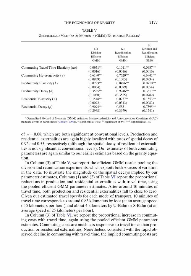
THE ECONOMICS OF DENSITY 2177
TABLE V
GENERALIZED METHOD OF MOMENTS (GMM) ESTIMATION RESULTSa
(3)(1) (2) Division and
Division Reunification ReunificationEfficient Efficient EfficientGMM GMM GMM
Commuting Travel Time Elasticity (κε) 0�0951∗∗∗ 0�1011∗∗∗ 0�0987∗∗∗
(0�0016) (0�0016) (0�0016)Commuting Heterogeneity (ε) 6�6190∗∗∗ 6�7620∗∗∗ 6�6941∗∗∗
(0�0939) (0�1005) (0�0934)Productivity Elasticity (λ) 0�0793∗∗∗ 0�0496∗∗∗ 0�0710∗∗∗
(0�0064) (0�0079) (0�0054)Productivity Decay (δ) 0�3585∗∗∗ 0�9246∗∗∗ 0�3617∗∗∗
(0�1030) (0�3525) (0�0782)Residential Elasticity (η) 0�1548∗∗∗ 0�0757∗∗ 0�1553∗∗∗
(0�0092) (0�0313) (0�0083)Residential Decay (ρ) 0�9094∗∗∗ 0�5531 0�7595∗∗∗
(0�2968) (0�3979) (0�1741)
aGeneralized Method of Moments (GMM) estimates. Heteroscedasticity and Autocorrelation Consistent (HAC)standard errors in parentheses (Conley (1999)). ∗ significant at 10%; ∗∗ significant at 5%; ∗∗∗ significant at 1%.
of η= 0�08, which are both significant at conventional levels. Production andresidential externalities are again highly localized with rates of spatial decay of0.92 and 0.55, respectively (although the spatial decay of residential externali-ties is not significant at conventional levels). Our estimates of both commutingparameters are again similar to our earlier estimates based on the gravity equa-tion.
In Column (3) of Table V, we report the efficient GMM results pooling thedivision and reunification experiments, which exploits both sources of variationin the data. To illustrate the magnitude of the spatial decays implied by ourparameter estimates, Columns (1) and (2) of Table VI report the proportionalreductions in production and residential externalities with travel time, usingthe pooled efficient GMM parameter estimates. After around 10 minutes oftravel time, both production and residential externalities fall to close to zero.Given our estimated travel speeds for each mode of transport, 10 minutes oftravel time corresponds to around 0.83 kilometers by foot (at an average speedof 5 kilometers per hour) and about 4 kilometers by U-Bahn or S-Bahn (at anaverage speed of 25 kilometers per hour).
In Column (3) of Table VI, we report the proportional increase in commut-ing costs with travel time, again using the pooled efficient GMM parameterestimates. Commuting costs are much less responsive to travel times than pro-duction or residential externalities. Nonetheless, consistent with the rapid ob-served decline in commuting with travel time, the implied commuting costs are
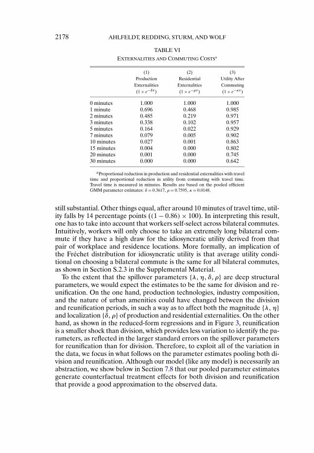
2178 AHLFELDT, REDDING, STURM, AND WOLF
TABLE VI
EXTERNALITIES AND COMMUTING COSTSa
(1) (2) (3)Production Residential Utility After
Externalities Externalities Commuting(1 × e−δτ) (1 × e−ρτ) (1 × e−κτ)
0 minutes 1�000 1�000 1�0001 minute 0�696 0�468 0�9852 minutes 0�485 0�219 0�9713 minutes 0�338 0�102 0�9575 minutes 0�164 0�022 0�9297 minutes 0�079 0�005 0�90210 minutes 0�027 0�001 0�86315 minutes 0�004 0�000 0�80220 minutes 0�001 0�000 0�74530 minutes 0�000 0�000 0�642
aProportional reduction in production and residential externalities with traveltime and proportional reduction in utility from commuting with travel time.Travel time is measured in minutes. Results are based on the pooled efficientGMM parameter estimates: δ= 0�3617, ρ= 0�7595, κ= 0�0148.
still substantial. Other things equal, after around 10 minutes of travel time, util-ity falls by 14 percentage points ((1 − 0�86)× 100). In interpreting this result,one has to take into account that workers self-select across bilateral commutes.Intuitively, workers will only choose to take an extremely long bilateral com-mute if they have a high draw for the idiosyncratic utility derived from thatpair of workplace and residence locations. More formally, an implication ofthe Fréchet distribution for idiosyncratic utility is that average utility condi-tional on choosing a bilateral commute is the same for all bilateral commutes,as shown in Section S.2.3 in the Supplemental Material.
To the extent that the spillover parameters {λ�η�δ�ρ} are deep structuralparameters, we would expect the estimates to be the same for division and re-unification. On the one hand, production technologies, industry composition,and the nature of urban amenities could have changed between the divisionand reunification periods, in such a way as to affect both the magnitude {λ�η}and localization {δ�ρ} of production and residential externalities. On the otherhand, as shown in the reduced-form regressions and in Figure 3, reunificationis a smaller shock than division, which provides less variation to identify the pa-rameters, as reflected in the larger standard errors on the spillover parametersfor reunification than for division. Therefore, to exploit all of the variation inthe data, we focus in what follows on the parameter estimates pooling both di-vision and reunification. Although our model (like any model) is necessarily anabstraction, we show below in Section 7.8 that our pooled parameter estimatesgenerate counterfactual treatment effects for both division and reunificationthat provide a good approximation to the observed data.
THE ECONOMICS OF DENSITY 2179
7.6. Comparison With Existing Estimates of Agglomeration Economies
Our central estimate of the elasticity of productivity with respect to pro-duction externalities (λ = 0�07 from Column (3) of Table V) is towards thehigh end of the 3–8 percent range stated in the survey by Rosenthal andStrange (2004), but less than the elasticities from some quasi-experimentalstudies (see, e.g., Kline and Moretti (2014) and Greenstone, Hornbeck, andMoretti (2010)).54 In comparing our results to the existing literature, a num-ber of points must be taken into account. First, the zero-profit condition (12)links overall productivity to wages and floor prices. Therefore, lower estimatesof agglomeration economies using data on wages, for example, could reflectthat higher productivity leads to both higher wages and higher floor prices.55
Second, our estimate of λ = 0�07 captures the effect of doubling workplaceemployment density holding constant travel times. In reality, a doubling in to-tal city population is typically achieved by a combination of an increase in thedensity of workplace employment and an expansion in geographical land area,with the accompanying increase in average travel times within the city. There-fore, the elasticity of productivity with respect to such a doubling of total citypopulation is less than λ = 0�07, because an increase in average travel timesreduces production externalities at a rate determined by the spatial decay pa-rameter δ.56
Our findings of substantial and highly localized production externalities arealso consistent with recent research using within-city data. Using data on thelocation of advertising agencies in Manhattan, Arzaghi and Henderson (2008)found little evidence of knowledge spillovers beyond 500 meters straight-linedistance. To compare straight-line distances to travel times, we computed themean travel time in 2006 across all bilateral connections in our data that covera straight-line distance between 450 and 550 meters, which is approximately
54In a recent meta-analysis of estimates of urban agglomeration economies, Melo, Graham,and Noland (2009) reported a mean estimate of 0.058 across 729 estimates from 34 studies, con-sistent with Rosenthal and Strange (2004).
55To further explore this point, we estimate elasticities of floor prices, wages, and productivitywith respect to distance from the pre-war CBD in 2006, which are −0�196, −0�130, and −0�143,respectively. Therefore, some of the higher productivity close to the CBD is reflected in higherfloor prices as well as in higher wages. The wage and productivity elasticities weighted by theircoefficients in zero-profits (12) add up to the floor price elasticity (up to rounding): −((0�8/0�2)×−0�130)+ ((1/0�2)× −0�143)= −0�195.
56To illustrate the quantitative relevance of this point, we have used the model to estimate themedian impact on the productivity of a West Berlin block within 3.75 kilometers of the pre-warCBD from production externalities from East Berlin in 1936, which corresponds to 0�0121 logpoints. In contrast, if one could distribute the workplace employment of East Berlin proportion-ately to each West Berlin block, this would increase workplace employment in each West Berlinblock by a factor of 1.7556, and hence from (20) would increase the productivity of each WestBerlin block by 0�0710 × ln(1�7556)= 0�0400 log points.
2180 AHLFELDT, REDDING, STURM, AND WOLF
9 minutes.57 After 9 minutes of travel time, our estimates suggest produc-tion externalities have declined to around 4 percent. Our estimates of pos-itive residential externalities are in line with the idea that urban amenitiesare endogenous to the surrounding concentration of economic activity, as inGlaeser, Kolko, and Saiz (2001) and Diamond (2013). Our findings of largeand highly localized residential externalities are consistent with other evidenceon spillovers in residential choices. Rossi-Hansberg, Sarte, and Owens (2010)used data on urban revitalization programs in Richmond, Virginia, and foundthat each dollar of home improvement spending generated between $2 and $6in land value by way of externalities in the targeted neighborhoods, but housingexternalities fall by approximately one half every 1,000 feet.
7.7. Over-Identification Checks
In addition to the over-identification checks using commuting data discussedabove, we now examine the model’s predictions for other variables not used inthe estimation. We begin with the ratio of floor space to land area. In our struc-tural estimation, we use the equilibrium relationships of the model to solve forthe adjusted density of development (ϕi) that equates the demand for floorspace to the supply of floor space. The resulting measure of the ratio of ad-justed floor space to land area (Li/Ki = ϕiK
−μi ) is implicitly quality adjusted
and captures other variables besides ϕi that enter the model isomorphicallythrough ϕi. In contrast, our measure of the ratio of floor space to land areain the data is coarse, because it is based on a number of discrete categories(e.g., greater than 4.5), and it does not control for the quality of floor space.Nonetheless, as reported in Table A.15 of the Technical Data Appendix, wefind a strong, statistically significant, and approximately log-linear relationshipbetween the two variables. For example, the estimated coefficient in 2006 isclose to 1 (0.959 with Conley standard error 0.018), with an R2 of 0.36. Giventhe caveats noted above, and the fact that this is a univariate regression usingcross-sectional micro data, the strength of this empirical relationship providesfurther support for the model’s predictions.
As an additional external validity check, we examine whether our estimatesof adjusted production and residential fundamentals {ai� bi} in 2006 are corre-lated with observable block characteristics that plausibly affect their suitabilityfor production or residence. As reported in Table A.16 of the Technical DataAppendix, we find that adjusted residential fundamentals are positively corre-lated with green areas, proximity to water, and listed buildings, and negativelycorrelated with noise and the level of destruction in the Second World War.In contrast, adjusted production fundamentals are uncorrelated with the level
57The standard deviation of travel times in the 450 to 550 meter straight-line distance bin is3.4 minutes, which illustrates that straight-line distances are an imperfect proxy for actual traveltimes in cities, particularly over shorter distances.
THE ECONOMICS OF DENSITY 2181
of noise, are less negatively correlated with the level of war-time destruction,and are positively correlated with the other observable block characteristics.Therefore, our estimates of adjusted production and residential fundamentalsare related in the expected way to separate data on observable correlates forthese variables.
7.8. Counterfactuals With Endogenous Location Characteristics
In Section 6.3, we reported counterfactuals for the special case of the modelwith exogenous location characteristics. In this subsection, we undertake coun-terfactuals for the model with agglomeration forces, in which productivity andamenities depend on endogenous production and residential externalities. Weassume alternative values of location characteristics {ai� bi� τij} or spillover pa-rameters {λ�δ�η�ρ} and solve for the model’s counterfactual equilibrium. Wefirst use these counterfactuals to provide further evidence on the model’s fit byexamining the extent to which the observed treatment effects of division andreunification can be explained by the model’s agglomeration and dispersionforces rather than by changes in location fundamentals. We next examine therelative importance of production and residential externalities. Finally, we re-port an out of sample counterfactual, in which we show that the model providesa framework that can be used to examine the impact of a change in transporttechnology.
As discussed above, in the presence of agglomeration forces, there is the po-tential for multiple equilibria in the model. We assume the equilibrium selec-tion rule of solving for the closest counterfactual equilibrium to the observedequilibrium prior to the counterfactual. In particular, we use the values ofthe endogenous variables from the observed equilibrium as our initial guessfor the counterfactual equilibrium.58 Our goal in these counterfactuals is notto determine the unique impact on economic activity, but rather to examinewhether the model with the estimated agglomeration parameters is capable ofgenerating counterfactual treatment effects for division and reunification closeto the observed treatment effects. In our structural estimation, the model ex-actly replicates the observed data, because we solve for the values of the struc-tural residuals for which the observed floor price and employment data arean equilibrium of the model. In contrast, in these counterfactuals, the model’spredictions need not necessarily replicate the observed data, because we as-sume alternative (counterfactual) values of location characteristics or parame-ters.
58Using these initial values, we solve the model’s system of equations for a new value of theendogenous variables. We then update our guess for the counterfactual equilibrium based on aweighted average of these new values and the initial values. Finally, we repeat this process untilthe new values and initial values converge.
2182 AHLFELDT, REDDING, STURM, AND WOLF
In our first counterfactual, we simulate division using our pooled parameterestimates and holding location fundamentals {ai� bi� ϕi} constant at their 1936values. We choose the reservation level of utility in the wider economy follow-ing division to ensure that the total population of West Berlin (H) is equal to itsvalue in the data in 1986. We estimate our baseline “difference-in-difference”specification (22) using the counterfactual change in floor prices following divi-sion. As reported in Column (1) of Table VII, we find counterfactual treatmenteffects of division close to the observed treatment effects (e.g., −0�836 for thefirst distance grid cell compared to −0�800 in Column (1) of Table I). There-fore, the estimated model with agglomeration forces can explain quantitativelythe observed impact of division, which suggests that our equilibrium selectionrule is selecting an equilibrium following division that is close to the observedequilibrium.
In Column (2), we set residential externalities to zero (η = 0). In Col-umn (3), we set production externalities to zero (λ = 0). As apparent fromthe table, both production and residential externalities make substantive con-tributions to the overall impact of division. In Column (4), we halve the ratesof spatial decay of both production externalities and residential externalities{δ�ρ}. In this case, we find somewhat larger counterfactual treatment effectsfor distance grid cells further from the pre-war CBD, consistent with the effectof division extending further into West Berlin.
In our next three counterfactuals, we simulate reunification, choosing thereservation level of utility in the wider economy following reunification to en-sure that the total population of Berlin (H) is equal to its value in the data in2006. We again estimate our baseline “difference-in-difference” specification(22) using the counterfactual change in floor prices. In Column (5), we use ourpooled parameter estimates, 1986 values of location fundamentals for WestBerlin, and 2006 values of location fundamentals for East Berlin. As shown inthe table, we find counterfactual treatment effects close to the observed treat-ment effects (e.g., 0.363 for the first distance grid cell compared to 0.398 inColumn (1) of Table II). Therefore, consistent with our results for division,the model with the estimated agglomeration forces can explain the observedimpact of reunification.
In Column (6), we consider the same specification as in Column (5), butuse 1936 (instead of 2006) values of location fundamentals for East Berlin.We now find counterfactual treatment effects substantially larger than the ob-served treatment effects (e.g., 1.160 versus 0.398 for the first distance grid cell).This pattern of results is consistent with the idea that a recovery of East Berlinto the relative levels of economic development prior to the Second World Warwould lead to a further reorientation of economic activity within West Berlin.In Column (7), we consider the same specification as in Column (5), but useour division (instead of pooled) parameter estimates. We find counterfactual
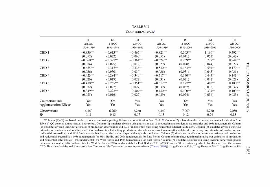
TH
EE
CO
NO
MIC
SO
FD
EN
SITY
2183TABLE VII
COUNTERFACTUALSa
(1) (2) (3) (4) (5) (6) (7)� ln QC � ln QC � ln QC � ln QC � ln QC � ln QC � ln QC
1936–1986 1936–1986 1936–1986 1936–1986 1986–2006 1986–2006 1986–2006
CBD 1 −0�836∗∗∗ −0�613∗∗∗ −0�467∗∗∗ −0�821∗∗∗ 0�363∗∗∗ 1�160∗∗∗ 0�392∗∗∗
(0�052) (0�032) (0�060) (0�051) (0�041) (0�052) (0�043)CBD 2 −0�560∗∗∗ −0�397∗∗∗ −0�364∗∗∗ −0�624∗∗∗ 0�239∗∗∗ 0�779∗∗∗ 0�244∗∗∗
(0�034) (0�025) (0�019) (0�029) (0�028) (0�044) (0�027)CBD 3 −0�455∗∗∗ −0�312∗∗∗ −0�336∗∗∗ −0�530∗∗∗ 0�163∗∗∗ 0�594∗∗∗ 0�179∗∗∗
(0�036) (0�030) (0�030) (0�036) (0�031) (0�045) (0�031)CBD 4 −0�423∗∗∗ −0�284∗∗∗ −0�340∗∗∗ −0�517∗∗∗ 0�140∗∗∗ 0�445∗∗∗ 0�143∗∗∗
(0�026) (0�019) (0�022) (0�031) (0�021) (0�042) (0�021)CBD 5 −0�418∗∗∗ −0�265∗∗∗ −0�351∗∗∗ −0�512∗∗∗ 0�177∗∗∗ 0�403∗∗∗ 0�180∗∗∗
(0�032) (0�022) (0�027) (0�039) (0�032) (0�038) (0�032)CBD 6 −0�349∗∗∗ −0�222∗∗∗ −0�304∗∗∗ −0�430∗∗∗ 0�100∗∗∗ 0�334∗∗∗ 0�103∗∗∗
(0�025) (0�016) (0�022) (0�029) (0�024) (0�034) (0�023)
Counterfactuals Yes Yes Yes Yes Yes Yes YesAgglomeration Effects Yes Yes Yes Yes Yes Yes Yes
Observations 6,260 6,260 6,260 6,260 7,050 6,260 7,050R2 0.11 0.13 0.07 0.13 0.12 0.24 0.13
aColumns (1)–(6) are based on the parameter estimates pooling division and reunification from Table V. Column (7) is based on the parameter estimates for division fromTable V. QC denotes counterfactual floor prices. Column (1) simulates division using our estimates of production and residential externalities and 1936 fundamentals. Column(2) simulates division using our estimates of production externalities and 1936 fundamentals but setting residential externalities to zero. Column (3) simulates division using ourestimates of residential externalities and 1936 fundamentals but setting production externalities to zero. Column (4) simulates division using our estimates of production andresidential externalities and 1936 fundamentals but halving their rates of spatial decay with travel time. Column (5) simulates reunification using our estimates of productionand residential externalities, 1986 fundamentals for West Berlin, and 2006 fundamentals for East Berlin. Column (6) simulates reunification using our estimates of productionand residential externalities, 1986 fundamentals for West Berlin and 1936 fundamentals for East Berlin. Column (7) simulates reunification using division rather than pooledparameter estimates, 1986 fundamentals for West Berlin, and 2006 fundamentals for East Berlin. CBD 1–CBD6 are six 500 m distance grid cells for distance from the pre-warCBD. Heteroscedasticity and Autocorrelation Consistent (HAC) standard errors in parentheses (Conley (1999)). ∗ significant at 10%; ∗∗ significant at 5%; ∗∗∗ significant at 1%.
2184 AHLFELDT, REDDING, STURM, AND WOLF
treatment effects for reunification close to those in Column (5), which is con-sistent with the similarity of the division and pooled parameter estimates.59
Although the focus of our analysis is on the division and reunification ofBerlin, our quantitative model provides a tractable platform for undertaking arange of counterfactuals. As an illustration of the model’s potential, our finalcounterfactual examines a change in transport technology. In particular, we ex-amine the impact of the automobile on the location of economic activity withinBerlin. We use the model to solve for the counterfactual equilibrium distribu-tion of economic activity in 2006 using travel time measures based solely onthe public transport network in 2006. To focus on the impact of the changein transport technology in Berlin, we hold the reservation utility in the widereconomy constant.
Our 2006 travel time measures using only public transport are typicallyhigher than our baseline 2006 measures that weight public transport and theautomobile by their modal shares. In comparison with American cities, thepublic transport network is far more extensive in Berlin (on average, publictransport, including walking and cycling, accounts for around two thirds ofjourneys in our 2006 data) and is relatively more important for commutinginto the central city. Table S.I of the Supplemental Material compares the ac-tual and counterfactual travel times. As shown in rows 1–4 of the table, the un-weighted average travel time across all possible bilateral connections with posi-tive values of either workplace or residence employment rises from 51 minutesto 70 minutes, and its standard deviation rises from 13 minutes to 26 minutes(since remote locations with high actual travel times and poor public transportconnections are most affected). As implied by our gravity equation estimationin Section 6.1, commuting flows are higher on average for shorter travel times.Therefore, as shown in rows 5–6 of the table, if we weight travel times by theactual bilateral commuting flows in the 2006 equilibrium, average travel timesrise from 32 minutes to 38 minutes.
The commuting technology facilitates a separation of workplace and resi-dence, enabling people to work in relatively high productivity locations (typi-cally in more central locations) and live in high amenity locations (typically insuburban locations). The deterioration of the commuting technology triggersan outflow of workers from Berlin, until floor prices fall such that expectedutility in Berlin is again equal to the unchanged reservation level of utility inthe wider economy. Total city employment and output fall by around 14 and
59While for brevity we concentrate on the model’s counterfactual predictions for the gradientof economic activity with respect to pre-war CBD, we find that it is also successful in accountingfor other features of the observed data, such as the gradient of economic activity with respectto the Kudamm. For example, regressing floor prices in West Berlin in 1986 and 2006 on gridcells of 500 meter intervals for distance to the Kudamm (and including grid cells for distance tothe pre-war CBD as controls), we find similar gradients of economic activity with respect to theKudamm for counterfactual floor prices as for actual floor prices.
THE ECONOMICS OF DENSITY 2185
12 percent, respectively (rows 7–8 of the table). Output falls by less than em-ployment, because labor is only one of the two factors of production and thetotal supply of floor space is held constant. On average, floor prices declineby 20 percent (row 9 of the table). This decline in floor prices is substantiallylarger for blocks experiencing above median increases in average unweightedtravel times (typically in remote locations) than for blocks experiencing belowmedian increases in these travel times (typically in more central locations), asshown in rows 10–11 of the table.
The general equilibrium response of the economy to the deterioration inthe commuting technology is that locations become less specialized in work-place and residence activity, as shown in Figure S.7 of the Supplemental Mate-rial. Panel A shows that blocks that are larger importers of commuters beforethe change in transport technology (larger net commuting on the horizon-tal axis) experience larger declines in workplace employment (on the verticalaxis). Panel B shows that blocks that are larger exporters of commuters beforethe change in transport technology (smaller net commuting on the horizon-tal axis) experience larger declines in residence employment (on the verticalaxis). A corollary of this decline in block specialization is a change in the pat-tern of worker sorting across bilateral pairs of workplace and residence loca-tions. Even though travel times for a typical bilateral pair have increased, wefind that this change in worker sorting results in average travel times weightedby commuting flows in the counterfactual equilibrium (row 12 of Table S.I)that marginally decline relative to average travel times weighted by commut-ing flows in the actual equilibrium (row 5 of the table). Taken together, theseresults highlight that the model provides a framework that can be used to an-alyze the endogenous change in the organization of economic activity withincities in response to changes in the transport network and other interventions(such as planning regulations).
8. CONCLUSIONS
In this paper, we develop a quantitative theoretical model of city structurethat incorporates agglomeration and dispersion forces, allows for asymmetriesin locational fundamentals, and remains tractable and amenable to empiri-cal analysis. To separate out agglomeration and dispersion forces from hetero-geneity in locational fundamentals, we combine the model with the exogenoussource of variation in the surrounding concentration of economic activity pro-vided by Berlin’s division and reunification.
The model implies a gravity equation for bilateral commuting flows, which issuccessful in accounting for observed commuting patterns. We find substantialdifferences in productivity and amenities across locations within cities that areendogenous to the surrounding concentration of economic activity. While ourestimates of the elasticity of productivity with respect to density using within-city data are somewhat higher than those using across-city data, we highlight
2186 AHLFELDT, REDDING, STURM, AND WOLF
the importance of taking into account the rapid spatial decay of production ex-ternalities when comparing estimates at different levels of spatial aggregation.We also find residential externalities of a comparable magnitude to productionexternalities.
We show that the special case of the model in which productivity and ameni-ties are exogenous is unable to account quantitatively for the observed treat-ment effects of division and reunification. In contrast, for the estimated valuesof agglomeration forces, the model is successful in accounting for these ob-served treatment effects. Although we use the natural experiment of Berlin toestimate the model’s parameters, our quantitative framework can be used toundertake counterfactuals for changes in the organization of economic activitywithin cities in response to other interventions, such as changes in the transportnetwork.
REFERENCES
AHLFELDT, G. M., S. J. REDDING, D. M. STURM, AND N. WOLF (2015): “Supplement to ‘TheEconomics of Density: Evidence From the Berlin Wall’,” Econometrica Supplemental Material,83, http://dx.doi.org/10.3982/ECTA10876. [2136,2143]
ALBOUY, D. (2008): “Are Big Cities Bad Places to Live? Estimating Quality of Life AcrossMetropolitan Areas,” Working Paper 14472, NBER. [2137]
ALONSO, W. (1964): Location and Land Use. Cambridge, MA: Harvard. [2131,2144]AMERICAN EMBASSY (1965): Handbook of Economic Statistics: Federal Republic of Germany and
Western Sectors of Berlin. Bonn: American Embassy. [2140]ARZAGHI, M., AND J. V. HENDERSON (2008): “Networking Off Madison Avenue,” Review of
Economic Studies, 75 (4), 1011–1038. [2132,2179]BAUM-SNOW, N. (2007): “Did Highways Cause Suburbanization?” Quarterly Journal of Eco-
nomics, 122 (2), 775–780. [2132]BERTRAND, M., E. DUFLO, AND S. MULLAINATHAN (2004): “How Much Should We Trust
Differences-in-Differences Estimators?” Quarterly Journal of Economics, 119 (1), 249–275.[2155]
BLEAKLEY, H., AND J. LIN (2012): “Portage and Path Dependence,” Quarterly Journal of Eco-nomics, 127 (2), 587–644. [2132]
BRINKMAN, J. (2013): “Congestion, Agglomeration, and the Structure of Cities,” Working Pa-per 13-25, Philadelphia Fed. [2131]
CICCONE, A., AND R. E. HALL (1996): “Productivity and the Density of Economic Activity,”American Economic Review, 86 (1), 54–70. [2132]
COMBES, P.-P., G. DURANTON, L. GOBILLON, AND S. ROUX (2010): “Estimating AgglomerationEconomies With History, Geology, and Worker Effects,” in Agglomeration Economies, ed. byE. L. Glaeser. Chicago: Chicago University Press. [2132]
COMBES, P.-P., G. DURANTON, AND L. GOBILLON (2014): “The Costs of Agglomeration: LandPrices in French Cities,” Report, Wharton. [2142,2167]
CONLEY, T. G. (1999): “GMM Estimation With Cross Sectional Dependence,” Journal of Econo-metrics, 92 (1), 1–45. [2153-2156,2158,2159,2169,2173,2177,2183]
DAVIS, D. R., AND D. E. WEINSTEIN (2002): “Bones, Bombs, and Break Points: The Geographyof Economic Activity,” American Economic Review, 92 (5), 1269–1289. [2132]
(2008): “A Search for Multiple Equilibria in Urban Industrial Structure,” Journal ofRegional Science, 48 (1), 29–65. [2132]
DAVIS, M. A., AND F. ORTALO-MAGNÉ (2011): “Housing Expenditures, Wages, Rents,” Review ofEconomic Dynamics, 14 (2), 248–261. [2137,2167]
THE ECONOMICS OF DENSITY 2187
DEKLE, R., AND J. EATON (1999): “Agglomeration and Land Rents: Evidence From the Prefec-tures,” Journal of Urban Economics, 46 (2), 200–214. [2132]
DIAMOND, R. (2013): “The Determinants and Welfare Implications of US Workers’ DivergingLocation Choices by Skill: 1980–2000,” Report, Stanford Graduate School of Business. [2180]
DONALDSON, D. (2015): “Railroads of the Raj: Estimating the Impact of Transportation Infras-tructure,” American Economic Review (forthcoming). [2132]
DURANTON, G., AND D. PUGA (2004): “Micro-Foundations of Urban AgglomerationEconomies,” in Handbook of Regional and Urban Economics, Vol. 4, ed. by J. V. Hendersonand J.-F. Thisse. Amsterdam: Elsevier, 2063–2117. [2131,2144]
DURANTON, G., AND M. A. TURNER (2011): “The Fundamental Law of Road Congestion: Evi-dence From US Cities,” American Economic Review, 101 (6), 2616–2652. [2166]
(2012): “Urban Growth and Transportation,” Review of Economic Studies, 79 (4),1407–1440. [2132]
EATON, J., AND S. KORTUM (2002): “Technology, Geography, and Trade,” Econometrica, 70 (5),1741–1779. [2131,2137,2168]
ELKINS, T. H., AND B. HOFMEISTER (1988): Berlin: Spatial Structure of a Divided City. London–New York: Methuen & Co. [2133]
EPPLE, D., B. GORDON, AND H. SIEG (2010): “A New Approach to Estimating the ProductionFunction for Housing,” American Economic Review, 100 (3), 905–924. [2142,2167]
FABER, B. (2015): “Trade Integration, Market Size, and Industrialization: Evidence from China’sNational Trunk Highway System,” Review of Economic Studies (forthcoming). [2132]
FEDER, G. (1939): Arbeitstätte—Wohnstätte. Schriftenreihe der Reichsarbeitsgemeinschaft fürRaumforschung an der Technischen Hochschule Berlin. Berlin: Julius Springer. [2166]
FORTHERINGHAM, S., AND M. O’KELLY (1989): Spatial Interaction Models: Formulations and Ap-plications. Dordrecht: Kluwer. [2164]
FRANKLIN, W. M. (1963): “Zonal Boundaries and Access to Berlin,” World Politics, 16 (1), 1–31.[2133]
FUJITA, M., AND P. KRUGMAN (1995): “When Is the Economy Monocentric? Von Thünen andChamberlain Unified,” Regional Science and Urban Economics, 25 (4), 505–528. [2131]
FUJITA, M., AND H. OGAWA (1982): “Multiple Equilibria and Structural Transformation of Non-Monocentric Urban Configurations,” Regional Science and Urban Economics, 12 (2), 161–196.[2131,2144]
GLAESER, E. L., AND D. C. MARE (2001): “Cities and Skills,” Journal of Labor Economics, 19 (2),316–342. [2132]
GLAESER, E. L., J. KOLKO, AND A. SAIZ (2001): “Consumer City,” Journal of Economic Geogra-phy, 1 (1), 27–50. [2180]
GREENSTONE, M., R. HORNBECK, AND E. MORETTI (2010): “Identifying AgglomerationSpillovers: Evidence From Winners and Losers of Large Plant Openings,” Journal of PoliticalEconomy, 118 (3), 536–598. [2132,2179]
GROGGER, J., AND G. HANSON (2011): “Income Maximization and the Selection and Sorting ofInternational Migrants,” Journal of Development Economics, 95 (1), 42–57. [2131]
HANSON, G. H. (1996): “Localization Economies, Vertical Organization, and Trade,” AmericanEconomic Review, 86 (5), 1266–1278. [2132]
(1997): “Increasing Returns, Trade, and the Regional Structure of Wages,” EconomicJournal, 107 (1), 113–133. [2132]
HEAD, K., AND T. MAYER (2014): “Gravity Equations: Workhorse, Toolkit, and Cookbook,” inHandbook of International Economics, Vol. 4, ed. by E. Helpman, G. Gopinath, and K. Rogoff.Amsterdam: Elsevier North Holland, 131–196. [2163]
HENDERSON, J. V., A. KUNCORO, AND M. TURNER (1995): “Industrial Development in Cities,”Journal of Political Economy, 103 (5), 1067–1085. [2132]
HERDEGEN, G. (1992): “Einstellungen zur Deutschen Einheit,” in Handwörterbuch zur DeutschenEinheit, Vol. 4, ed. by W. Weidenfeld and K.-R. Korte. Frankfurt am Main: Campus Verlag.[2135]

2188 AHLFELDT, REDDING, STURM, AND WOLF
KALWEIT, F. (1929): Die Baustellenwerte in Berlin 1928. Berlin: Emro. [2150](1937): Die Baustellenwerte in Berlin: Strassen-Verzeichnis, Neubearbeitung Abgeschlossen
am 30. Juni 1936. Berlin: Carl Heymanns. [2150]KENNAN, J., AND J. R. WALKER (2011): “The Effect of Expected Income on Individual Migration
Decisions,” Econometrica, 79 (1), 211–251. [2131]KLINE, P., AND E. MORETTI (2014): “Local Economic Development, Agglomeration Economies,
and the Big Push: 100 Years of Evidence From the Tennessee Valley Authority,” QuarterlyJournal of Economics, 129 (1), 275–331. [2132,2179]
LAMBRECHT, H., AND H. TISCHNER (1969): Der Handel West-Berlins mit der DDR und Osteuropa:Probleme und Möglichkeiten. Berlin: Deutsches Institut für Wirtschaftsforschung. [2134]
LEYDEN, F. (1933): Gross-Berlin: Geographie einer Weltstadt. Berlin: Gebr. Mann Verlag. [2150]LUCAS, R. E. (2000): “Externalities and Cities,” Review of Economic Dynamics, 4 (2), 245–274.
[2144]LUCAS, R. E., AND E. ROSSI-HANSBERG (2002): “On the Internal Structure of Cities,” Econo-
metrica, 70 (4), 1445–1476. [2131]MARSHALL, A. (1920): Principles of Economics. London: Macmillan. [2128]MCARTHUR, D. P., G. KLEPPE, I. THORSEN, AND J. UBOE (2011): “The Spatial Transferability of
Parameters in a Gravity Model of Commuting Flows,” Journal of Transport Geography, 19 (4),596–605. [2164]
MCDONALD, J., AND D. MCMILLEN (2010): Urban Economics and Real Estate: Theory and Policy.Hoboken, NJ: John Wiley & Sons. [2164]
MCFADDEN, D. (1974): “The Measurement of Urban Travel Demand,” Journal of Public Eco-nomics, 3 (4), 303–328. [2131,2137]
MELO, P. C., D. J. GRAHAM, AND R. B. NOLAND (2009): “A Meta-Analysis of Estimates of UrbanAgglomeration Economies,” Regional Science and Urban Economics, 39 (3), 332–342. [2179]
MICHAELS, G. (2008): “The Effect of Trade on the Demand for Skill: Evidence From the Inter-state Highway System,” Review of Economics and Statistics, 90 (4), 683–701. [2132]
MILLS, E. S. (1967): “An Aggregative Model of Resource Allocation in a Metropolitan Centre,”American Economic Review, 57 (2), 197–210. [2131,2144]
MORETTI, E. (2004): “Workers’ Education, Spillovers and Productivity: Evidence From Plant-Level Production Functions,” American Economic Review, 94, 656–690. [2132]
(2011): “Local Labor Markets,” in Handbook of Labor Economics, Vol. 4b, ed. byD. Card and O. Ashenfelter. Amsterdam: Elsevier North Holland, 1238–1303. [2132]
MUTH, R. (1969): Cities and Housing. Chicago: University of Chicago Press. [2131,2144]OFFICE FOR STATISTICS BERLIN-BRANDENBURG (2007): Statistical Yearbook of Berlin. Berlin:
Office for Statistics Berlin-Brandenburg. [2148]RAUCH, J. E. (1993): “Productivity Gains From Geographic Concentration of Human Capital,”
Journal of Urban Economics, 34 (3), 380–400. [2132]REDDING, S. J., AND D. M. STURM (2008): “The Costs of Remoteness: Evidence From German
Division and Reunification,” American Economic Review, 98 (5), 1766–1797. [2132]REDDING, S. J., D. M. STURM, AND N. WOLF (2011): “History and Industry Location: Evidence
From German Airports,” Review of Economics and Statistics, 93 (3), 814–831. [2132]ROBACK, J. (1982): “Wages, Rents and the Quality of Life,” Journal of Political Economy, 90 (6),
1257–1278. [2132,2137]ROGGENBUCH, F. (2008): Das Berliner Grenzgängerproblem. Verflechtung und Systemkonkurrenz
vor dem Mauerbau. Berlin–New York: Walter de Gruyter. [2134]ROSENTHAL, S. S., AND W. C. STRANGE (2004): “Evidence on the Nature and Sources of Ag-
glomeration Economics,” in Handbook of Regional and Urban Economics, Vol. 4, ed. by J. V.Henderson and J. F. Thisse. Amsterdam: Elsevier North Holland. [2131,2179]
(2008): “The Attenuation of Human Capital Spillovers,” Journal of Urban Economics,64 (2), 373–389. [2132]
ROSSI-HANSBERG, E., P.-D. SARTE, AND R. I. OWENS (2010): “Housing Externalities,” Journal ofPolitical Economy, 118 (3), 485–535. [2132,2180]

THE ECONOMICS OF DENSITY 2189
SHARP, T. (1975): The Wartime Alliance and the Zonal Division of Germany. Oxford: ClarendonPress. [2133]
SVEIKAUSKAS, L. A. (1975): “The Productivity of Cities,” Quarterly Journal of Economics, 89 (3),393–413. [2132,2144]
TIMOTHY, D., AND W. C. WHEATON (2001): “Intra-Urban Wage Variation, Employment Loca-tion, and Commuting Times,” Journal of Urban Economics, 50 (2), 338–366. [2168]
VALENTINYI, Á., AND B. HERRENDORF (2008): “Measuring Factor Income Shares at the SectoralLevel,” Review of Economic Dynamics, 11 (4), 820–835. [2167]
Dept. of Geography and Environment, London School of Economics, Hough-ton Street, London, WC2A 2AE, U.K. and CEPR; [email protected],
WWS and Dept. of Economics, Princeton University, Fisher Hall, Princeton, NJ08540, U.S.A., NBER, and CEPR; [email protected],
Dept. of Economics, London School of Economics, Houghton Street, London,WC2A 2AE, U.K. and CEPR; [email protected],
andDept. of Economics, Humboldt University, Spandauer Strasse 1, 10178 Berlin,
Germany and CEPR; [email protected].
Manuscript received June, 2012; final revision received February, 2015.


![COUNTER MEMORIALS Hoheisel [Berlin-Kassel-Buchenwald] Ullman [Berlin] Eisenman/Happold [Berlin] Gerz [Harburg/Saarbrucken]](https://img.pdfslide.us/doc/110x75/56649f135503460f94c27537/counter-memorials-hoheisel-berlin-kassel-buchenwald-ullman-berlin-eisenmanhappold.jpg)