THE ECONOMIC IMPACTS OF THE PRISON ...povertyinamerica.mit.edu/products/publications/prison...Economic Impacts of the Prison Development Boom Farrigan and Glasmeier 1 INTRODUCTION

THE ECONOMIC IMPACTS OF THE PRISON DEVELOPMENT BOOM ON PERSISTENTLY POOR RURAL PLACES

by

Tracey L. Farrigan Research Assistant

Department of Geography The Pennsylvania State University

107 Walker Building University Park, PA 16802

[email protected]

and

Amy K. Glasmeier Professor of Geography and Regional Planning

Department of Geography The Pennsylvania State University

308 Walker Building University Park, PA 16802

[email protected]

Key Words: rural development, prisons, persistent poverty, quasi-experimental methods Abstract: Prison construction was a noticeable component of economic development initiatives in rural places during the 1980s and the 1990s. Yet, few comprehensive ex post-empirical studies have been conducted and therefore the literature remains inconclusive about the economic impacts of prisons. Following a temporal overview of the geography of prison development and associated characteristics, this research employs quasi-experimental control group methods to examine the effects of state-run prisons, constructed in rural places between 1985 and 1995, on county earnings by employment sector, population, poverty rate, and degree of economic health. Our analysis suggests that prisons have had no significant economic effect on rural places in general, but that they may have had a positive impact on poverty rates in persistently poor rural counties, while also associated with diminishing transfer payments and increasing state and local government earnings in places with relatively good economic health. However, we found little evidence to support the conclusion that prison impacts were significant enough to foster structural economic change. This research was supported by a grant from the Ford Foundation and was conducted at the Earth and Mineral Sciences Environmental Institute at The Pennsylvania State University.

Economic Impacts of the Prison Development Boom Farrigan and Glasmeier

1

INTRODUCTION

Many rural areas have persistently high poverty rates and have continuously lagged

behind the rest of the nation economically. Few economic development strategies have been

shown to ameliorate this trend. Therefore, rural communities seeking alternatives to improve

their situation have often turned to recruiting enterprises that are considered the least desirable

elsewhere, such as prisons (Thies 2000). Rural prison facilities, although smaller than their urban

counterparts, are generally large in comparison to base populations in rural places (Beale 1996).

Hence, in most instances it is expected that prison construction and subsequent operations will

create relatively significant direct impacts through prison employment and indirect impacts by

way of regional multiplier effects. However, empirical evidence that demonstrates the economic

effects of prison sitings in rural places is sorely lacking, and moreso is evidence in support of

prisons’ impacts on economically distressed places and their resident poverty populations.

The lack of analysis is due in part to the fact that measuring the economic effects of

prison development is made difficult by varying pre-existing characteristics of places and the

regions in which they are situated, such as the degree of economic diversity within the economy

and the extent of inter-industry and inter-regional linkages. In conjunction, it is understood that

the characteristics of the prison facility must be taken into consideration; the composition of

facility expenditures, including number of employees and related skill levels and wages rates, all

need to be evaluated. Yet, many argue that even if attempts to capture such factors are made, as

when seeking to generalize impacts via an input-output analysis or conjoined econometric

analysis, those efforts are fruitless because prisons are economic “islands” (Rephann 1996). That

is, they are isolated from their host communities in both their hiring and expenditure practices,

offering little beyond a physical presence that serves as a negative externality in attempting to

attract other enterprises to the area (Carlson 1992; Shichor 1992).

Compositional characteristics of such investment often limit their economic development

impact. For instance, prison employment policies and educational requirements often result in

administrative and corrections positions being filled from within the corrections system by

transfers of individuals from outside the community. These employees tend to commute to work

rather than relocate (Beale 1993, 1996; Fitchen 1991). Job opportunities for area residents are

typically comprised of clerical positions and skilled service work. These jobs tend to pay


2

significantly lower wage rates than the more skilled, professional jobs. Thus, prisons are not

thought to have much impact on welfare and poverty populations; in general, high-skilled jobs

are taken by individuals originating outside the local community while the prison population

itself provides ample low-skilled labor to fulfill menial tasks. Prisoners accumulate records of

good behavior as part of their work details, earn nominal compensation for certain tasks, while

receiving some level of training (Fitchen 1991). Additionally, most of the prisons constructed in

rural places over the last several decades are owned and operated by the state or federal

government or national private industry, therefore prison inputs and purchasing networks are at

the national scale (Sechrest 1992). These factors suggest that not only do few jobs go to

residents, but also the indirect benefit of the prison as an economic activity is limited, as

substantial forms of leakage may go hand in hand with prison development.

Yet, despite the potential limitations in the benefits derived locally from prisons, many

rural places took advantage of the opportunity to bid for and acquire a prison during the prison-

building boom that began in the 1980s and lasted through the late 1990s (Beale 1993, 1996;

Beck and Harrison 2001). Laws such as “three strikes and you’re out” and longer and more

severe prison terms for first time drug-related offenses led to an exponential increase in state

level prison populations. Some states, and regions within them, made prison location into a

business. Descriptive analysis of prison locations over the last two decades clearly show that in

some regions of the country, prison siting became a target of development opportunity. The

purpose of this analysis, therefore, is to provide a measure of impact of state prisons, developed

at the height of the boom (1985–1995), on diverse rural places, particularly those with high

levels of poverty and economic distress prior to prison construction.

This paper includes two parts. The first part of the paper describes the spatial and

temporal distribution of prisons in the United States. A unique data set was created that allows

for the tracking of prison construction in the U.S. to 1995 and the examination of the

characteristics of those prisons in terms of the type of facility, its location, attributes of the prison

population, and conjoint location of prison facilities. Thus, the first part provides a detailed

snapshot of the spatial economic of incarceration in the United States. The second part of the

paper presents an analysis of the effect of prison construction on county-level economic

conditions. In this analysis we emphasize the effect such investments have on populations at risk


3

as measured by changes in the poverty population and area-wide economic health in matching

counties. In doing so, we first report on the theoretical models applied in order to make explicit

the main assumptions of the research project and to relate the methods to the reader on a higher

level of abstraction than is traditionally the case in the reporting of impact assessment (Becker

and Porter 1986).

PART I: THE SPATIAL & TEMPORAL DISTRIBUTION OF PRISONS IN THE U.S.

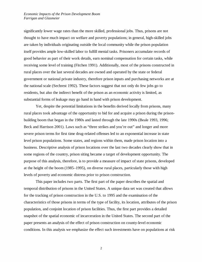
The growth in the number of federal, state, private, and joint local authority prison

facilities in operation in the United States as of 1995 is described with reference to three distinct

periods of spatial development: pre-1945, 1945–1984, and 1985–1995. All are illustrated by year

of original construction in Figure 1, where the acceleration in prison sitings over time and

periodic shifts are made evident by the change in the slope of the line. This is particularly clear

for the latter period, during what has become known as “the prison development boom”, which is

represented at the tail end of the graph, from about the 60th percentile on.

Figure 1. Cumulative Percent of Prisons by Year of Construction: 1778–1995

Prison Facility Location. Nearly 36 percent of the prisons in operation in 1995 were

constructed from 1985–1995, with an average of 48 new prisons per year for the 11-year period.

As in the prior two periods, the majority of those prisons were constructed in the South, mainly

0

20

40

60

80

100

120

1778

1850

1871

1882

1891

1900

1908

1915

1922

1929

1936

1943

1951

1958

1965

1972

1979

1986

1993

year

per

cent


4

in South Atlantic states, such as North Carolina prior to 1945 and in Florida from 1945–1995.

However, the pattern of growth from 1985 to 1995 shifted substantially from the South Atlantic

Division of the South to the West South Central, concentrating in Texas with 14.4 percent of the

growth for that period (more than double that of any other state). These and other dominant

patterns of prison construction, including a boost in prison sitings in California from 1945–1984

and in Michigan from 1985–1995, can be seen by comparing Figures 2–4

Among the nearly 1,500 prisons included in our data set, 39 percent or 576 facilities are

located in rural places as currently defined,1 mainly in North Carolina, New York, and California

(see Figure 5). Of that 39 percent, 36 percent were constructed from 1985–1995 alone and are

somewhat concentrated in Michigan (9%), New York (7%), Texas (6%), and Connecticut (6%).

Rural prisons constructed in earlier periods are more highly concentrated and located in southern

places. For instance, the highest percentages go to Virginia (10.5%), Florida, and California

(10.3% each) for 1945–1984 and to North Carolina (21.5%) for pre-1945 construction.

Therefore, the older the rural prison, the greater the tendency for it to be located in the Southeast,

while newly constructed rural prisons are more widely dispersed across the United States.

Facilities in urban places have a similar geography for the earlier periods, but the more newly

constructed the urban prison the more likely it is to be located in Texas. Texas went from

housing 3.8 percent of all new urban prison locations for 1945–1984 to 19.6 percent of those

constructed during the prison development boom, while no other state showed similarly

significant growth in urban prison sitings from 1985–1995.

Prison Facility and Population Characteristics. Beyond the patterns of change in the

location of newly constructed prison facilities in the United States, there has been little change in

their character. For instance, prisons in the U.S. have historically been and are currently

dominated by state-operated, minimum-security facilities that are authorized to house male

inmates only. These characteristics were jointly held by 29 percent of the total number of prisons

in operation in 1995, which were predominately located in North Carolina (10.4%). However, it

should be noted that although new prison sitings during the boom were almost entirely state-run

(80%), there were a slight shift with respect to past periods toward the construction of federal

1 Here we use 2000 Census Bureau definitions of urban areas and urban centers to identify rural places (in 2000 the Census Bureau changed the urban designation from a place-based definition to one using these concepts). In Part II,


5

maximum- and minimum-security prisons. There was also a greater degree of segregation by

gender authorization from 1985–1995 than in the earlier periods of prison growth and a

significant reduction in the percent of prisons under court order limiting the maximum number of

inmates with an associated reduction in the absolute number allowed. In reference to the latter,

based on dates of original construction, that number went from an average of 167 inmates per

restricted facility, which was 25 percent of all prisons constructed pre-1945, to 116 inmates for

the 15 percent restricted for 1945–1984 constructions, to 54 inmates for the 7 percent restricted

for 1985–1995.

Overall, at the time of the count used in this study (June 30, 1995), the United States

prison population was characterized by an average total of 690 inmates per facility (668 for the

average annual daily population). Among them, the percentage of black/African American

inmates (47%) was slightly higher than that for white inmates (41%), with very few inmates of

other racial categories besides Hispanic, Puerto Rican, Cuban, or others of Spanish decent

(11%). Additionally, inmates under 18 made up less than one percent of the total and male

inmates outweighed female nine to one. However, there was a distinct geography of gender and

race between rural and urban prison facilities, with rural prisons holding higher percentages of

male and black/African American inmates than their urban counterparts in 1995. Likewise, urban

prison facilities held higher percentages of female and white inmates than rural prisons. This

pattern was similar regardless of regional location or age of the facility, except in the case of

inmates of Hispanic, Puerto Rican, Cuban, or others of Spanish decent, whom were equally

represented in urban and rural prisons, but tended to be located more so in newer urban prisons.

That pattern was found to be correlated with the growth in prison construction in Texas from

1985–1995 in places currently designated as urban.

Prison Employment Characteristics. On average, prison facilities in 1995 supported

226 full- and part-time payroll staff and the highest-paying, most skill-dependent occupations

(professional, correctional, and administrative) made up nearly 87 percent of those positions.

There was little difference between those numbers based on urban and rural facilities, but the

number of full- and part-time payroll staff did vary when combined with regional location. For

instance, the average for rural facilities in the Northeast was the largest (311 staff) followed by

for the county-based analysis, rural is defined by a subset of non-metro ERS County Typology Codes (1993 Beale


6

urban facilities in the Northeast (288 staff). Further, the count for urban/Midwest was slightly

larger than that for rural/Midwest and the opposite was true for urban and rural facilities in the

South, while the average number of staff for urban facilities in the West was nearly double that

of rural prisons in the West. This suggests that when average employment is used as the measure

of facility size, regional location is necessary to give meaning to urban and rural distinctions.2

Adding the dimension of time further complicates generalizations, but lends support to prior

findings with regard to urban and rural differences that suggest that urban prisons tend to be

larger in size than rural (e.g. Beale 1996). For instance, when looking at prisons constructed

during the 1985–1995 period alone, urban facilities emerge as those with the highest average

number of staff overall and in all regions except the Midwest.

Considering location and both the gender and race of prison facility staff in 1995, the

greatest percentage by far was white males, as has historically been the case, but with a greater

degree of gender and racial diversity in urban prisons than in rural locations. In urban prisons the

highest percentage of non-male staff members were found in facilities in Nebraska and New

Hampshire (28% each), while the highest percentage of non-white staff were reported for urban

facilities in Colorado, California, and Texas (approximately 67% each). Once again, a correlation

was found with those of Hispanic, Puerto Rican, Cuban, or others of Spanish descent, who

tended to be staffed moreso in new urban prisons in Texas than elsewhere.

Looking further at occupational characteristics, first by gender and then in conjunction

with location, we found that in 1995 both males and females predominately worked in

corrections occupations (an average of 71% and 41%, respectively), followed by professional

(9%) and maintenance (7%) for males and clerical (25%) and professional for females (20%).3

Although grave disparities existed between male and female staff for corrections occupations

when considering the percentage of total full- and part-time staff (approximately 4:1 in urban

facilities and 5:1 in rural facilities), women were almost equally represented in professional

codes 7, 8, and 9). 2 In past prison studies, the number of employees and inmates has commonly been used together as the measure of facility size and the result has been that rural prisons were found to be smaller than urban prisons. The failure of this study to support that finding may be due to the reliance on employment as the sole measure, but it is more likely due to the fact that prior studies have also tended to rely on county-level designations of urban and rural (i.e. based on metro and non-metro county classifications) rather than place-level designations (i.e. the community rather than the county in which the facility is located) as we have here. 3 Taken as a percent of total male and total female full- and part-time staff independently. Data by race were not available.


7

occupations across both urban and rural facility locations overall. Additionally, females

represented a higher share of professional occupations in urban facilities in the Northeast and

South as well as in rural facilities in the South.

Finally, in relation to lower-skilled (and lower-wage) jobs and their availability to the

local labor market considering potential competition from prison inmates, it is interesting to note

that the majority of facilities support work assignments for inmates and do so in diverse

occupations, although more generally in farming/agriculture. In 1995, 93 percent reported having

inmates on work assignments, with an average of 206 per facility. Considering this and the

number of jobs supplied by prisons on average (226) and the percent in higher-skilled

occupations (87%) in 1995, the notion that prisons provide a sufficient supply of labor internally

to fill the low-skilled positions created by the facility’s existence, thereby eliminating access to

those jobs for area residents, seems likely. This leads the way into the second part of the paper

and our primary task, which is to construct a measure of impact of prison development from

1985–1995 with a focus on persistently poor rural places.

PART II: THE IMPACTS OF RURAL STATE-PRISON DEVELOPMENT

The techniques typically used for economic impact analysis vary considerably (Pleeter

1980). Yet all impact analyses are based on the assumption that a project or treatment, such as

the development of a prison in a persistently poor rural place for the sake of economic growth,

triggers organizational, population group, and project environment effects and side-effects that

can be assessed to some extent (Becker and Porter 1986). In this case, it is assumed that there is a

causal link between the prison’s activities and economic impacts and that measurable effects

occur by means of direct or indirect distributive processes. This simplistic idea of cause-and-

effect forms the analytical basis of impact analysis, even though scientifically, the impact of a

specific development like a prison can be measured only if it is known what the situation would

have been if that prison had never been constructed (Isserman and Merrifield 1987). Therefore, it

has to be demonstrated that changes in the dependent variables (prison impacts) are due to the

independent variables (prison operation)—accordingly, a distinction must be made between the

gross and net impacts of a prison (Neubert 2000).


8

Preliminary Considerations. Theoretically, net impacts can be arrived at by isolating

the endogenous disturbance variables––those associated with the prison operation itself––from

exogenous disturbances. The effects that are extraneous to the prison. Yet realistically, clear

distinctions as such are made impossible by the embeddedness of the factors of interest to social

scientists in complex, heterogeneous socioeconomic and spatial structures with implicit

counterfactual (unobserved) qualities that lead to logical contradictions or misleading inferences

when ignored (Kaufman and Cooper 1999). Therefore, scientific research as such can only be

conducted in social laboratory experiments, where hypothetical approaches to causal inference

that capture counterfactual contrasts are applied.

For instance, the social experiment method, which employs experimental data (e.g.

Heckman et al. 1997; LaLonde 1986), allows for the construction of a control group from a

randomized subset of a potential comparison population. Other advantages are discussed at

length in Bassi (1984) and Hausman and Wise (1985), but in fact, social experiments are hardly

feasible and often of questionable benefit; they are expensive to implement, are not amenable to

extrapolation (i.e. not easily applicable to ex-ante analysis), and are typically limited by the

ruling out of spillover, substitution, displacement, and equilibrium effects by requiring that the

control group be completely unaffected by the treatment (Blundell and Costa-Dias 2002). As

such, social experiments are rarely used in economics and geography.

Still, if a more realistic measure of impact is to be achieved, then comparison of

situations with and without the treatment (whether cross-sectional, counterfactual, or

longitudinal) is the most important and comprehensible element of evaluation (Neubert 2000).

Yet, comparative examination necessitates reduction to a subset of relevant information (e.g.

economic properties of the prison facility and/or the location) and explicit assessment objectives,

thereby producing an estimate of effects given definitional “if… then” statements (Davis 1990).

Thus, impact analysis is best understood not as a true measure of effect, but rather as a study

designed to generate quantitative estimates based on a conditional model.

Quasi-Experimental Design. Both natural experiment and quasi-experimental

approaches to impact analysis are based on comparison of treatment and non-treatment groups.

The natural experiment design, commonly employing the “difference in difference” method,

examines the differences between the average behavioral properties of a naturally occurring


9

control (non-treatment) group and the treatment group. This measure can be used in the absence

of a genuine randomized control group as well, in a quasi-experimental format whereby

comparison group selection is determined with respect to the most important variables as defined

by the researcher. In this situation the selection process is dependent on two critical assumptions

that make comparison group selection extremely difficult (Blundell and Costa-Dias 2002, p. 3):

(1) common time effects across groups and (2) no systematic composition changes within each

group.

In other words, the matching of groups for comparison is done by selecting sufficient

observable factors, where sufficiency is determined by hypothetical or statistical controls, and

analysis is conducted on the basis that any two places with similar factor values will not display

systematic differences in behavior when faced with the same treatment. The logic behind quasi-

experimental analysis, therefore, is that a control group can be selected non-randomly to serve as

the baseline from which inferences about change to treated places––in this case places in which a

state prison was constructed, can be made. Although control group assignment is non-random,

certain aspects of a true experimental design are reconstructed in the analytical process thereby

approximating a randomized trial. As such, quasi-experimental designs offer an alternative in the

absence of randomized controls, but they are disadvantaged by the potential loss of internal

validity through the selection process.

Quasi-experimental design presupposes that qualitative comparability exists prior to

treatment and that the impacts of treatment exposure would be the same for both groups when

realistically the same outcome is rarely, if ever achieved, particularly due to heterogeneous

external influences (Neubert 2000). Yet, quasi-experimental designs have been shown to be

“sufficiently probing…well worth employing where more efficient probes are unavailable”

(Campbell and Stanley 1963, p. 35, author’s emphasis). As such, efforts to improve evaluations

of the effectiveness of policies or projects intended to foster economic change in specific places

have increasingly led to the application of quasi-experimental control group approaches to

impact assessment (Cook and Campbell 1979; Isserman and Beaumont 1989; Isserman and

Merrifield 1982; Reed and Rogers 2001). For example, quasi-experimental designs have been

used in the evaluation of regional employment subsidies (Bohm and Lind 1993), for measuring

the impacts of highways in rural areas (Broder et al. 1992; Rogers and Marshment 2000), and for


10

determining the economic effects of the Appalachian Regional Commission (Isserman and

Rephann 1995), among other economic development and infrastructure investment initiatives.

Mahalanobis Metric Matching. A number of acceptable analytical alternatives exist

within the quasi-experimental framework; “no one method dominates… [t]he most appropriate

choice of evaluation method has been shown to depend on a combination of the data available

and the policy parameter of interest” (Blundell and Costa Dias 2002, p. 32).4 Accordingly, a

variety of matching techniques are used to pair treated observations with non-treated controls

based on background covariates (e.g. population and income growth rates) that are defined by the

researcher based on their study relevance. However, the most extensively documented of those

techniques is Mahalanobis metric matching.

Mahalanobis metric matching is commonly done by randomly ordering the treatment

observations, then calculating the distance between the first treated observation and all of the

control or non-treated observations, where distance d(i,j), between treated observation i and

control subject j is defined by the Mahalanobis distance (u – v)TC-1(u – v) (D’Agostino 1998).

Here, u and v are the values of matching variables for the treated subject i, control subject j, and

C is the sample covariance matrix of the matching variables from the full control group. The

process that follows the calculation of the Mahalanobis distance is that the control observation

with the minimum Mahalanobis distance is selected to match the first ordered treatment

observation. Then, both are removed from their respective groups as a match and the process is

repeated until all matches to treatment observations are made.

The major limitation of this technique is that as the number of covariates included in the

specified model increases, it becomes more and more difficult to find relatively close matches.

This is due to the fact that the calculated Mahalanobis distance expands with the number of

dimensions in the analysis and therefore the average distance between observations tends to

become larger as well. The reason is that significant differences often exist between covariates of

4 Quasi-experimental design refers to a broad research approach, consisting of a variety and often combined techniques, generally selected on the basis of the situation being examined, the factors of interest, data restrictions, and the comfort of the researcher with the form of analysis, assumptions and associated issues of validity. For review: Blundell and Costa-Dias (2002) offer a summary of matching and instrumental variable quasi-experimental methods as well as a comparison to social and natural experiments. Campbell and Stanley (1963) provide a detailed survey of the strengths and weaknesses of a collection of heterogeneous quasi-experimental, true experiment, and correlational and ex post facto designs. Also see Heckman and Hotz (1989) and Reed and Rogers (2001) for choice among methods with respect to social and economic policy impact analysis in particular.


11

the treatment and non-treatment group in observational studies, perfect matches rarely if ever

exist; as such, the more extensive the model, the greater the likely error of comparison. These

differences or errors can lead to biased estimates; therefore, they must be adjusted for in order to

reduce selection bias prior to determining the treatment effect.

Reducing Bias with Propensity Scores. A measure that can easily be added to the

process in order to solve the bias problem is the propensity score. This metric allows for the

simultaneous matching of covariates on a single variable and is defined as the conditional

probability of receiving a treatment given specified observed covariates e(X) = pr(Z = 1 � X),

implying that Z and X are conditionally independent given e(X) (Rosenbaum and Rubin 1985). In

other words, the propensity score is a value between zero and one that represents the predicted

probability of the dependent variable. If the dependent variable is a treatment group, as with this

study on rural places in which state prisons were opened during the prison development boom,

then the propensity score would be interpreted as the predicted probability of acquiring a prison

for each case based on the combined pre-treatment characteristics of the county, as defined by

the covariates selected for the study.

The propensity score can be estimated using logistic regression or discriminant analysis.

The latter requires the assumption that the covariates have a multivariate normal distribution

while the former does not, but the results in both cases can be used similarly to adjust the

measure of the treatment effect, thereby increasing the confidence level that approximately

unbiased estimates are obtained (D’Agostino 1998). However, a number of approaches can be

employed to reduce bias and increase precision using propensity scores. One is a case-control

matched analysis performed in conjunction with the propensity score, another is nearest available

matching on the estimated propensity score, and a number of other variations exist, many of

which include the Mahalanobis metric (Parsons 2000; Rosenbaum and Rubin 1984; Rubin 1979;

Rubin and Thomas 1996).

Having examined a number of techniques, Rosenbaum and Rubin (1985) concluded that

the nearest available Mahalanobis metric matching within calipers defined by the propensity

score was the best choice. Their decision was based on the technique’s balance between the

covariates for the treated and control or non-treated groups in addition to a balance between the

squared covariates and the cross products between the two groups. This is achieved by


12

combining the Mahalanobis metric matching and propensity score methods, constraining the

control group to a preset amount of the treated observation’s estimated propensity score

(D’Agostino 1998). This is explained further in the next section with reference to the current

study.

Study Methodology. The major requirement in statistical matching is to preserve the

marginal distributions of the variables in their original form. To satisfy this condition,

constrained matching is the method most commonly used (Rodgers 1984). In this analysis

selection of both treatment and control or non-treatment groups were constrained initially by

sequential calipers that serve as proxies for spatial independence (Isserman and Merrifield 1987).

In the case of the treatment group, rural places in either completely rural counties or counties

with an urban population of less than 20,000 not adjacent to a metro area were identified. Within

that pool of potential treatment counties, those with one state-run prison constructed between

1985 and 1995 were selected for analysis (see Table 1). The pre-treatment control group was

similarly chosen, with non-metropolitan county designations meeting the same urban/rural

population criteria and the lack of, or presence of “0,” state-run prisons within the county

boundaries.

Since economic impacts on the treatment areas’ economies as a whole as well as on their

poverty population were of interest, the model covariates were specified as measures of growth,

industrial structure, and population and demand (Isserman and Rephann 1995; Rephann et al.

1997; Rephann and Isserman 1994). Income shares by major industries (excluding mining where

data suppression is a serious problem) serve as measures of industrial structure; change rates in

economic health,5 poverty, population, and total personal income as measures of growth; and,

proportions of residential adjustment and transfer income, and state and local earnings as

measures of population and demand (see Table 2).

5 Based on an index developed by Glasmeier and Fuellhart (1999) that incorporates measures of unemployment, labor force participation, and dependency rates.


13

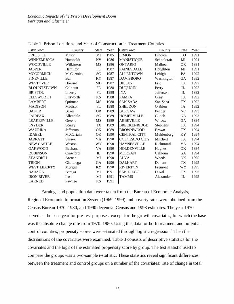
Table 1. Prison Locations and Year of Construction in Treatment Counties

Earnings and population data were taken from the Bureau of Economic Analysis,

Regional Economic Information System (1969–1999) and poverty rates were obtained from the

Census Bureau 1970, 1980, and 1990 decennial Census and 1998 estimates. The year 1970

served as the base year for pre-test purposes, except for the growth covariates, for which the base

was the absolute change rate from 1970–1980. Using this data for both treatment and potential

control counties, propensity scores were estimated through logistic regression.6 Then the

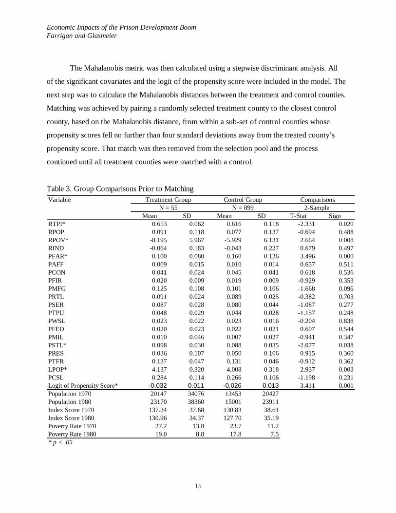
distributions of the covariates were examined. Table 3 consists of descriptive statistics for the

covariates and the logit of the estimated propensity score by group. The test statistic used to

compare the groups was a two-sample t-statistic. These statistics reveal significant differences

between the treatment and control groups on a number of the covariates: rate of change in total

City/Town County State Year City/Town County State YearFREESOIL Mason MI 1985 LIMON Lincoln CO 1991WINNEMUCCA Humboldt NV 1986 MANISTIQUE Schoolcraft MI 1991WOODVILLE Wilkinson MS 1986 ONTARIO Malheur OR 1991JASPER Hamilton FL 1987 PAINESDALE Houghton MI 1991MCCORMICK McCormick SC 1987 ALLENTOWN Lehigh PA 1992PINEVILLE Bell KY 1987 DAVISBORO Washington GA 1992WESTOVER Howard MD 1987 DILLEY Frio TX 1992BLOUNTSTOWN Calhoun FL 1988 DUQUOIN Perry IL 1992BRISTOL Liberty FL 1988 INA Jefferson IL 1992ELLSWORTH Ellsworth KS 1988 PAMPA Gray TX 1992LAMBERT Quitman MS 1988 SAN SABA San Saba TX 1992MADISON Madison FL 1988 SHELDON O'Brien IA 1992BAKER Baker OR 1989 BURGAW Pender NC 1993FAIRFAX Allendale SC 1989 HOMERVILLE Clinch GA 1993LEAKESVILLE Greene MS 1989 ABBEVILLE Wilcox GA 1994SNYDER Scurry TX 1989 BRECKENRIDGE Stephens TX 1994WAURIKA Jefferson OK 1989 BROWNWOOD Brown TX 1994IDABEL McCurtain OK 1990 CENTRAL CITY Muhlenberg KY 1994JARRATT Sussex VA 1990 COLORADO CITY Mitchell TX 1994NEW CASTLE Weston WY 1990 HAYNESVILLE Richmond VA 1994OAKWOOD Buchanan VA 1990 HOLDENVILLE Hughes OK 1994ROBINSON Crawford IL 1990 MORGAN Calhoun GA 1994STANDISH Arenac MI 1990 ALVA Woods OK 1995TRION Chattooga GA 1990 DALHART Dallam TX 1995WEST LIBERTY Morgan KY 1990 RIVERTON Fremont WY 1995BARAGA Baraga MI 1991 SAN DIEGO Duval TX 1995IRON RIVER Iron MI 1991 TAMMS Alexander IL 1995LARNED Pawnee KS 1991


14

personal income (RTPI) and poverty (RPOV), proportion of farming (PFAR) and state and local

government earnings (PSTL), and population (LPOP).

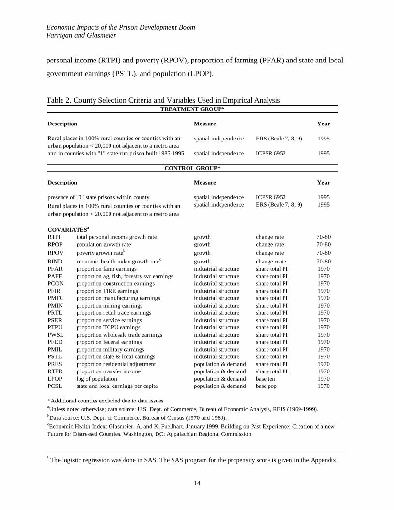
Table 2. County Selection Criteria and Variables Used in Empirical Analysis

6 The logistic regression was done in SAS. The SAS program for the propensity score is given in the Appendix.

Description Measure Year

spatial independence ERS (Beale 7, 8, 9) 1995

and in counties with "1" state-run prison built 1985-1995 spatial independence ICPSR 6953 1995

Description Measure Year

presence of "0" state prisons within county spatial independence ICPSR 6953 1995spatial independence ERS (Beale 7, 8, 9) 1995

COVARIATESa

RTPI total personal income growth rate growth change rate 70-80RPOP population growth rate growth change rate 70-80

RPOV poverty growth rateb growth change rate 70-80

RIND economic health index growth ratec growth change reate 70-80PFAR proportion farm earnings industrial structure share total PI 1970PAFF proportion ag, fish, forestry svc earnings industrial structure share total PI 1970PCON proportion construction earnings industrial structure share total PI 1970PFIR proportion FIRE earnings industrial structure share total PI 1970PMFG proportion manufacturing earnings industrial structure share total PI 1970PMIN proportion mining earnings industrial structure share total PI 1970PRTL proportion retail trade earnings industrial structure share total PI 1970PSER proportion service earnings industrial structure share total PI 1970PTPU proportion TCPU earnings industrial structure share total PI 1970PWSL proportion wholesale trade earnings industrial structure share total PI 1970PFED proportion federal earnings industrial structure share total PI 1970PMIL proportion military earnings industrial structure share total PI 1970PSTL proportion state & local earnings industrial structure share total PI 1970PRES proportion residential adjustment population & demand share total PI 1970RTFR proportion transfer income population & demand share total PI 1970LPOP log of population population & demand base ten 1970PCSL state and local earnings per capita population & demand base pop 1970

*Additional counties excluded due to data issuesaUnless noted otherwise; data source: U.S. Dept. of Commerce, Bureau of Economic Analysis, REIS (1969-1999).bData source: U.S. Dept. of Commerce, Bureau of Census (1970 and 1980).

CONTROL GROUP*

TREATMENT GROUP*

cEconomic Health Index: Glasmeier, A. and K. Fuellhart. January 1999. Building on Past Experience: Creation of a new Future for Distressed Counties. Washington, DC: Appalachian Regional Commission

Rural places in 100% rural counties or counties with an urban population < 20,000 not adjacent to a metro area

Rural places in 100% rural counties or counties with an urban population < 20,000 not adjacent to a metro area


15

The Mahalanobis metric was then calculated using a stepwise discriminant analysis. All

of the significant covariates and the logit of the propensity score were included in the model. The

next step was to calculate the Mahalanobis distances between the treatment and control counties.

Matching was achieved by pairing a randomly selected treatment county to the closest control

county, based on the Mahalanobis distance, from within a sub-set of control counties whose

propensity scores fell no further than four standard deviations away from the treated county’s

propensity score. That match was then removed from the selection pool and the process

continued until all treatment counties were matched with a control.

Table 3. Group Comparisons Prior to Matching

Variable

Mean SD Mean SD T-Stat Sign RTPI* 0.653 0.062 0.616 0.118 -2.331 0.020RPOP 0.091 0.118 0.077 0.137 -0.694 0.488RPOV* -8.195 5.967 -5.929 6.131 2.664 0.008RIND -0.064 0.183 -0.043 0.227 0.679 0.497PFAR* 0.100 0.080 0.160 0.126 3.496 0.000PAFF 0.009 0.015 0.010 0.014 0.657 0.511PCON 0.041 0.024 0.045 0.041 0.618 0.536PFIR 0.020 0.009 0.019 0.009 -0.929 0.353PMFG 0.125 0.108 0.101 0.106 -1.668 0.096PRTL 0.091 0.024 0.089 0.025 -0.382 0.703PSER 0.087 0.028 0.080 0.044 -1.087 0.277PTPU 0.048 0.029 0.044 0.028 -1.157 0.248PWSL 0.023 0.022 0.023 0.016 -0.204 0.838PFED 0.020 0.023 0.022 0.021 0.607 0.544PMIL 0.010 0.046 0.007 0.027 -0.941 0.347PSTL* 0.098 0.030 0.088 0.035 -2.077 0.038PRES 0.036 0.107 0.050 0.106 0.915 0.360PTFR 0.137 0.047 0.131 0.046 -0.912 0.362LPOP* 4.137 0.320 4.008 0.318 -2.937 0.003PCSL 0.284 0.114 0.266 0.106 -1.198 0.231Logit of Propensity Score* -0.032 0.011 -0.026 0.013 3.411 0.001Population 1970 20147 34076 13453 20427Population 1980 23170 38360 15001 23911Index Score 1970 137.34 37.68 130.83 38.61Index Score 1980 130.96 34.37 127.70 35.19Poverty Rate 1970 27.2 13.8 23.7 11.2Poverty Rate 1980 19.0 8.8 17.8 7.5* p < .05

Comparisons2-Sample N = 55 N = 899

Treatment Group Control Group


16

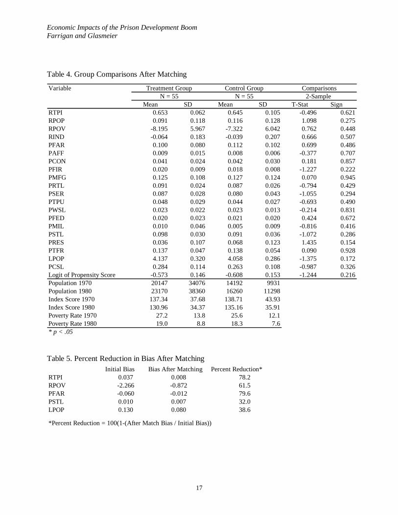
Once matching was completed t-tests were run on the matched counties to examine

whether or not the bias between the groups had been removed. Table 4 contains the descriptive

statistics and t-tests for the after matching comparisons. As exhibited by the calculated means

and lack of significance, the matched sample covariates were relatively evenly distributed.

Further evidence of bias reduction is given in Table 5, which shows percent reduction in bias for

the covariates with the largest initial biases, such as the poverty growth rate (RPOV) for which

the bias was reduced by 61.5 percent. Essentially, no significant differences remain, therefore the

matched control group was deemed satisfactory. Hence, the quasi-randomized experiment was

successfully created and the covariates could be likened to the background variables in

randomized experiments.

Example Matched County. Before describing the results of our analysis, we present

select characteristics of an example matched county that we will track as a way of making clearer

both the procedure and the results that follow. Pender County, North Carolina was the site of the

construction of an 808 inmate, medium-security prison in 1993. Prior to the construction of the

prison, at the close of the pre-treatment period (1980), the county’s population was 22,333 and

the poverty rate was 21.3 percent. The per capita transfer payment level was $2,447 and the

average earnings per job were $20,465 (both in 2000 dollars). The economic base of the county

was in the farming sector, which held 20.8 percent of total full- and part-time employment in

1980. Since 1980, the following changes occurred statistically over time (absolute change from

1980 to 1999): 84 percent population increase, 7.7 poverty rate decrease, 61.4 percent per capita

transfer payment increase, 2.6 percent average earnings per job increase, and 15.1 percent

farming sector employment decrease. During the same period of time Pender’s control county

(Choctaw, OK) witnessed a 10.6 percent population decrease, a 1.7 percent decrease in the

poverty rate, 36.5 percent growth in per capita transfer payments, and a 27.7 percent decrease in

average earnings per job. There was also a minimal .4 percent decrease in farm employment,

which was similarly the dominant employment sector in 1980.

Identification of Prison Impacts. The post-treatment period was estimated from 1980–

1999 (except 1997 for index scores and 1998 for poverty rates),7 thereby allowing for a

7 These were the latest dates for which data were available for these measures at the time this study was completed.


17

Table 4. Group Comparisons After Matching

Table 5. Percent Reduction in Bias After Matching

Initial Bias Bias After Matching Percent Reduction*RTPI 0.037 0.008 78.2RPOV -2.266 -0.872 61.5PFAR -0.060 -0.012 79.6PSTL 0.010 0.007 32.0LPOP 0.130 0.080 38.6

*Percent Reduction = 100(1-(After Match Bias / Initial Bias))

Variable

Mean SD Mean SD T-Stat Sign RTPI 0.653 0.062 0.645 0.105 -0.496 0.621RPOP 0.091 0.118 0.116 0.128 1.098 0.275RPOV -8.195 5.967 -7.322 6.042 0.762 0.448RIND -0.064 0.183 -0.039 0.207 0.666 0.507PFAR 0.100 0.080 0.112 0.102 0.699 0.486PAFF 0.009 0.015 0.008 0.006 -0.377 0.707PCON 0.041 0.024 0.042 0.030 0.181 0.857PFIR 0.020 0.009 0.018 0.008 -1.227 0.222PMFG 0.125 0.108 0.127 0.124 0.070 0.945PRTL 0.091 0.024 0.087 0.026 -0.794 0.429PSER 0.087 0.028 0.080 0.043 -1.055 0.294PTPU 0.048 0.029 0.044 0.027 -0.693 0.490PWSL 0.023 0.022 0.023 0.013 -0.214 0.831PFED 0.020 0.023 0.021 0.020 0.424 0.672PMIL 0.010 0.046 0.005 0.009 -0.816 0.416PSTL 0.098 0.030 0.091 0.036 -1.072 0.286PRES 0.036 0.107 0.068 0.123 1.435 0.154PTFR 0.137 0.047 0.138 0.054 0.090 0.928LPOP 4.137 0.320 4.058 0.286 -1.375 0.172PCSL 0.284 0.114 0.263 0.108 -0.987 0.326Logit of Propensity Score -0.573 0.146 -0.608 0.153 -1.244 0.216Population 1970 20147 34076 14192 9931Population 1980 23170 38360 16260 11298Index Score 1970 137.34 37.68 138.71 43.93Index Score 1980 130.96 34.37 135.16 35.91Poverty Rate 1970 27.2 13.8 25.6 12.1Poverty Rate 1980 19.0 8.8 18.3 7.6* p < .05

Comparisons2-Sample N = 55 N = 55

Treatment Group Control Group


18

maximum of five years for potential construction effects prior to the date of facility completion.

A series of paired samples t-tests were run on the cumulative change rates for each of the

covariates by group based on the following data select cases: all, economic health index rank 1

or 2 for 1980, economic health index rank 3 or 4 1980, poverty rate 1980 less than 20 percent,

poverty rate 1980 greater than or equal to 20 percent, and poverty rate 1980 greater than 30

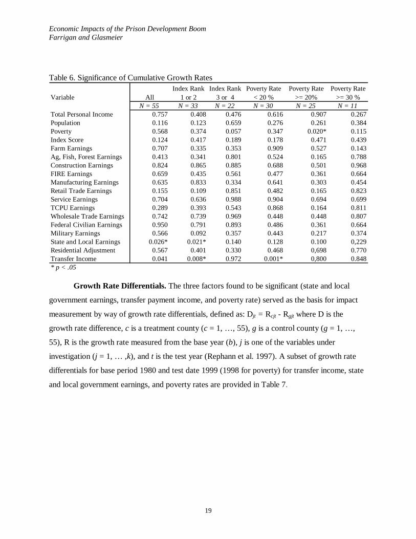
percent.8 The “all” category test was meant to identify whether or not significant differences in

the mean values of the 55 treated counties and their control counties developed during the post-

treatment period. None of the factors examined were shown to be significantly different except

for state and local government earnings (see Table 6). That is, on the average there was a

noticeable difference in the positive growth in state and local government earnings between

treatment counties and their controls, thereby suggesting that prison development was

responsible for that difference.

The other tests were conducted in order to stratify the treatment county sample by

economically distressed (index rank 3 or 4)/non-distressed counties (index rank 1 or 2) and

persistently poor (poverty rate => 20%) / not persistently poor counties (poverty rate < 20%) at

the start of the impact period. Significant differences were not found to exist between treatment

and control counties in any of the categories, except for change in transfer income and state and

local earnings for counties with an index rank of one or two in 1980; change in transfer payment

income for treatment counties with a poverty rate less than 20 percent; and change in poverty

rates for treatment counties with poverty rates equal to or above 20 percent in 1980. This

suggests that prison impacts on economically distressed or persistently poor counties were

limited to poverty rate effects for persistently poor counties. Further, counties impacted were

likely not to be the most extremely poor given the lack of significant difference in change in

poverty rates for counties in the 30 percent or greater range.

8 The poverty rate category >=20% includes those counties that are in the >=30% range; otherwise all categories , both index rank and poverty rate, are mutually exclusive.


19

Table 6. Significance of Cumulative Growth Rates

Growth Rate Differentials. The three factors found to be significant (state and local

government earnings, transfer payment income, and poverty rate) served as the basis for impact

measurement by way of growth rate differentials, defined as: Djt = Rcjt - Rgjt where D is the

growth rate difference, c is a treatment county (c = 1, …, 55), g is a control county (g = 1, …,

55), R is the growth rate measured from the base year (b), j is one of the variables under

investigation (j = 1, … ,k), and t is the test year (Rephann et al. 1997). A subset of growth rate

differentials for base period 1980 and test date 1999 (1998 for poverty) for transfer income, state

and local government earnings, and poverty rates are provided in Table 7.

Variable AllIndex Rank

1 or 2Index Rank

3 or 4Poverty Rate

< 20 %Poverty Rate

>= 20%Poverty Rate

>= 30 %N = 55 N = 33 N = 22 N = 30 N = 25 N = 11

Total Personal Income 0.757 0.408 0.476 0.616 0.907 0.267Population 0.116 0.123 0.659 0.276 0.261 0.384Poverty 0.568 0.374 0.057 0.347 0.020* 0.115Index Score 0.124 0.417 0.189 0.178 0.471 0.439Farm Earnings 0.707 0.335 0.353 0.909 0.527 0.143Ag, Fish, Forest Earnings 0.413 0.341 0.801 0.524 0.165 0.788Construction Earnings 0.824 0.865 0.885 0.688 0.501 0.968FIRE Earnings 0.659 0.435 0.561 0.477 0.361 0.664Manufacturing Earnings 0.635 0.833 0.334 0.641 0.303 0.454Retail Trade Earnings 0.155 0.109 0.851 0.482 0.165 0.823Service Earnings 0.704 0.636 0.988 0.904 0.694 0.699TCPU Earnings 0.289 0.393 0.543 0.868 0.164 0.811Wholesale Trade Earnings 0.742 0.739 0.969 0.448 0.448 0.807Federal Civilian Earnings 0.950 0.791 0.893 0.486 0.361 0.664Military Earnings 0.566 0.092 0.357 0.443 0.217 0.374State and Local Earnings 0.026* 0.021* 0.140 0.128 0.100 0,229Residential Adjustment 0.567 0.401 0.330 0.468 0,698 0.770Transfer Income 0.041 0.008* 0.972 0.001* 0,800 0.848* p < .05


20

Table 7. Growth Rate Differentials; Treatment Counties; Index Rank 1 or 2 and Poverty Rate => 20; 1980–1999

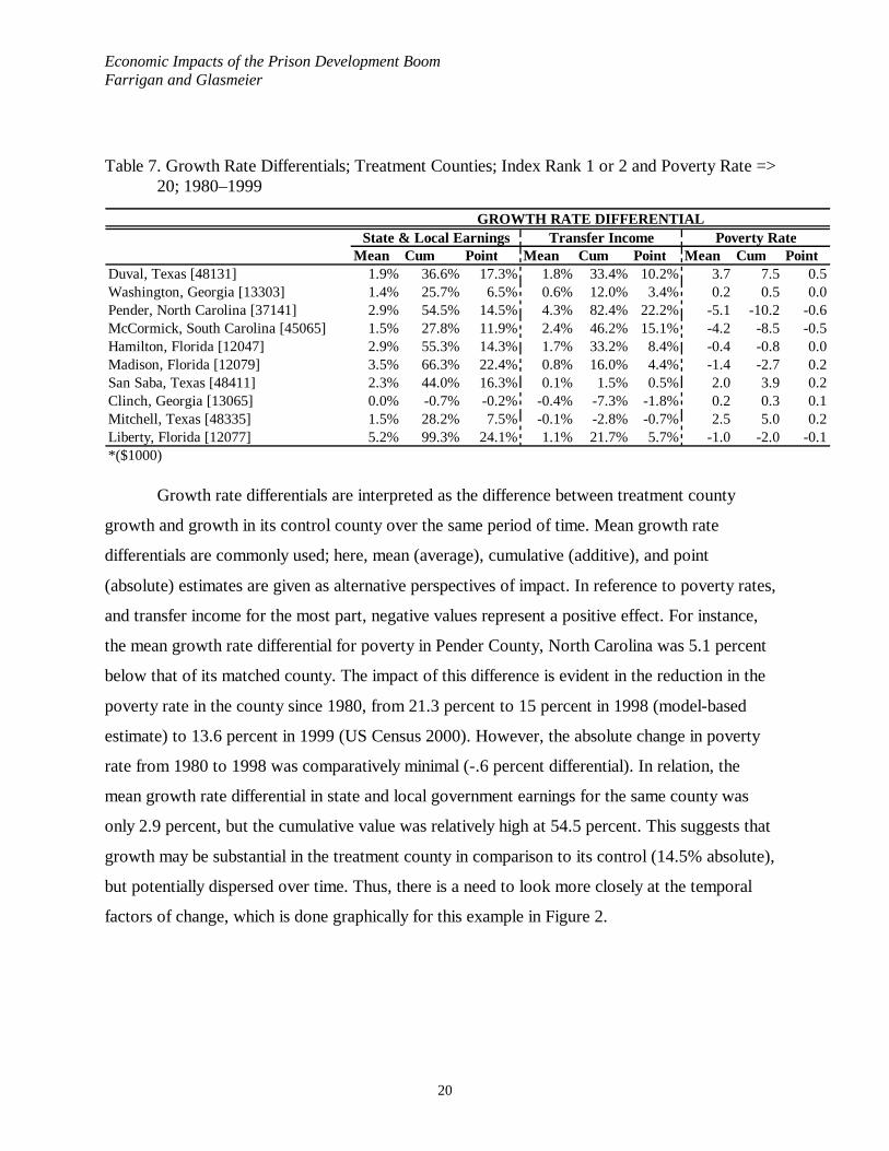
Growth rate differentials are interpreted as the difference between treatment county

growth and growth in its control county over the same period of time. Mean growth rate

differentials are commonly used; here, mean (average), cumulative (additive), and point

(absolute) estimates are given as alternative perspectives of impact. In reference to poverty rates,

and transfer income for the most part, negative values represent a positive effect. For instance,

the mean growth rate differential for poverty in Pender County, North Carolina was 5.1 percent

below that of its matched county. The impact of this difference is evident in the reduction in the

poverty rate in the county since 1980, from 21.3 percent to 15 percent in 1998 (model-based

estimate) to 13.6 percent in 1999 (US Census 2000). However, the absolute change in poverty

rate from 1980 to 1998 was comparatively minimal (-.6 percent differential). In relation, the

mean growth rate differential in state and local government earnings for the same county was

only 2.9 percent, but the cumulative value was relatively high at 54.5 percent. This suggests that

growth may be substantial in the treatment county in comparison to its control (14.5% absolute),

but potentially dispersed over time. Thus, there is a need to look more closely at the temporal

factors of change, which is done graphically for this example in Figure 2.

Mean Cum Point Mean Cum Point Mean Cum PointDuval, Texas [48131] 1.9% 36.6% 17.3% 1.8% 33.4% 10.2% 3.7 7.5 0.5Washington, Georgia [13303] 1.4% 25.7% 6.5% 0.6% 12.0% 3.4% 0.2 0.5 0.0Pender, North Carolina [37141] 2.9% 54.5% 14.5% 4.3% 82.4% 22.2% -5.1 -10.2 -0.6McCormick, South Carolina [45065] 1.5% 27.8% 11.9% 2.4% 46.2% 15.1% -4.2 -8.5 -0.5Hamilton, Florida [12047] 2.9% 55.3% 14.3% 1.7% 33.2% 8.4% -0.4 -0.8 0.0Madison, Florida [12079] 3.5% 66.3% 22.4% 0.8% 16.0% 4.4% -1.4 -2.7 0.2San Saba, Texas [48411] 2.3% 44.0% 16.3% 0.1% 1.5% 0.5% 2.0 3.9 0.2Clinch, Georgia [13065] 0.0% -0.7% -0.2% -0.4% -7.3% -1.8% 0.2 0.3 0.1Mitchell, Texas [48335] 1.5% 28.2% 7.5% -0.1% -2.8% -0.7% 2.5 5.0 0.2Liberty, Florida [12077] 5.2% 99.3% 24.1% 1.1% 21.7% 5.7% -1.0 -2.0 -0.1*($1000)

GROWTH RATE DIFFERENTIALState & Local Earnings Transfer Income Poverty Rate


21

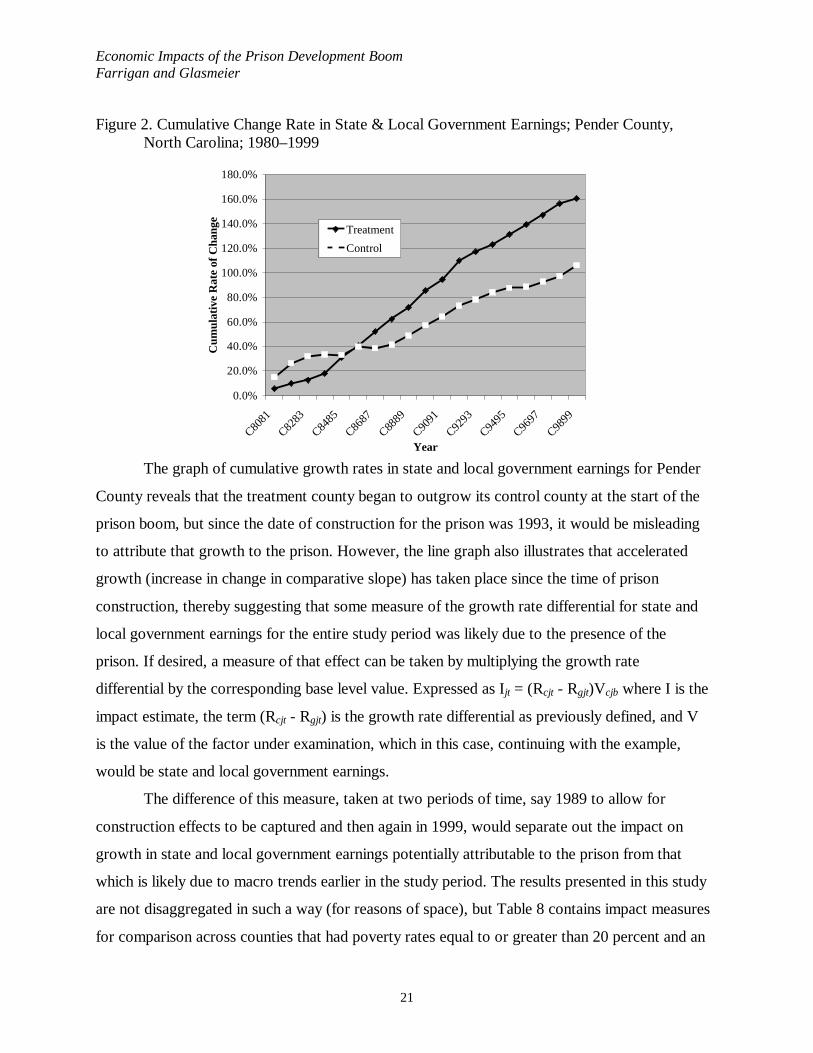
Figure 2. Cumulative Change Rate in State & Local Government Earnings; Pender County, North Carolina; 1980–1999

The graph of cumulative growth rates in state and local government earnings for Pender

County reveals that the treatment county began to outgrow its control county at the start of the

prison boom, but since the date of construction for the prison was 1993, it would be misleading

to attribute that growth to the prison. However, the line graph also illustrates that accelerated

growth (increase in change in comparative slope) has taken place since the time of prison

construction, thereby suggesting that some measure of the growth rate differential for state and

local government earnings for the entire study period was likely due to the presence of the

prison. If desired, a measure of that effect can be taken by multiplying the growth rate

differential by the corresponding base level value. Expressed as Ijt = (Rcjt - Rgjt)Vcjb where I is the

impact estimate, the term (Rcjt - Rgjt) is the growth rate differential as previously defined, and V

is the value of the factor under examination, which in this case, continuing with the example,

would be state and local government earnings.

The difference of this measure, taken at two periods of time, say 1989 to allow for

construction effects to be captured and then again in 1999, would separate out the impact on

growth in state and local government earnings potentially attributable to the prison from that

which is likely due to macro trends earlier in the study period. The results presented in this study

are not disaggregated in such a way (for reasons of space), but Table 8 contains impact measures

for comparison across counties that had poverty rates equal to or greater than 20 percent and an

0.0%

20.0%

40.0%

60.0%

80.0%

100.0%

120.0%

140.0%

160.0%

180.0%

C8081

C8283

C8485

C8687

C8889

C9091

C9293

C9495

C9697

C9899

Year

Cum

ulat

ive

Rat

e of

Cha

nge

Treatment

Control


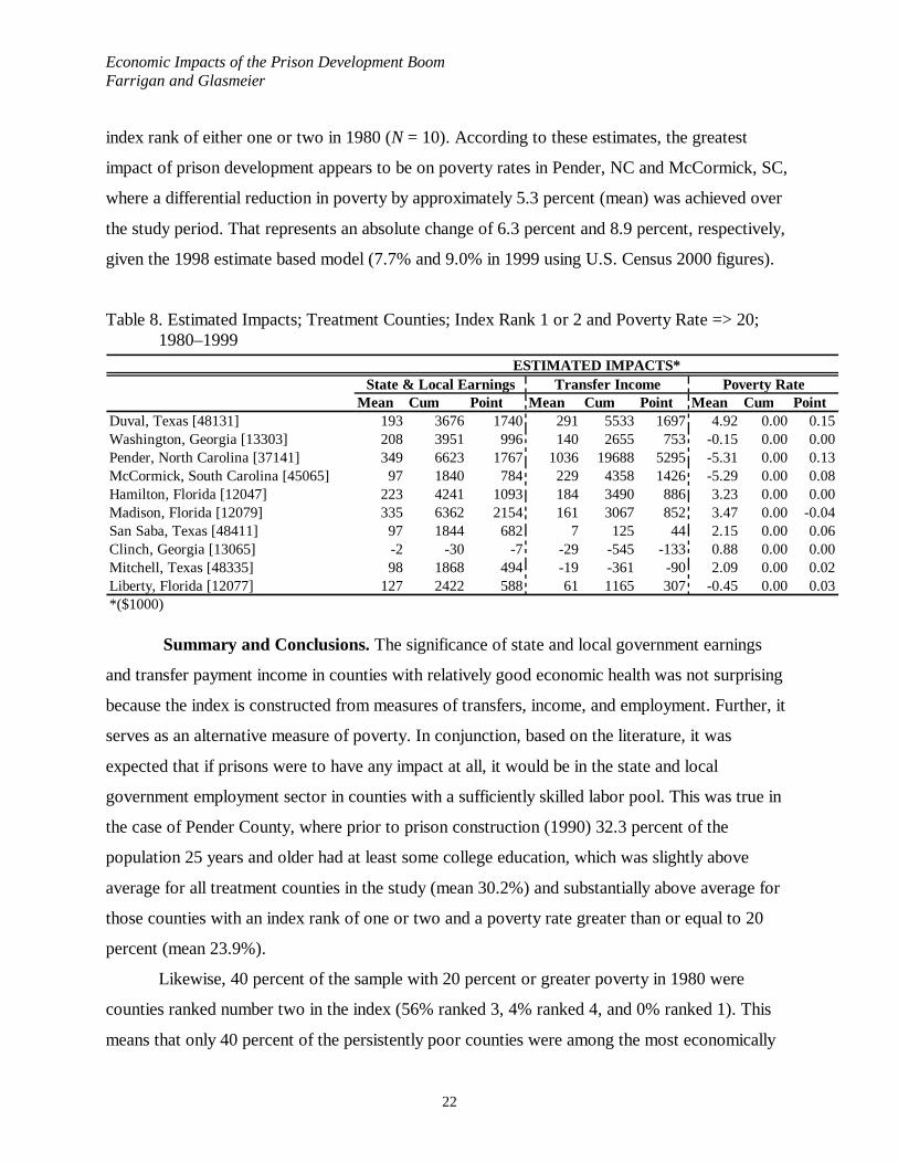
22

index rank of either one or two in 1980 (N = 10). According to these estimates, the greatest

impact of prison development appears to be on poverty rates in Pender, NC and McCormick, SC,

where a differential reduction in poverty by approximately 5.3 percent (mean) was achieved over

the study period. That represents an absolute change of 6.3 percent and 8.9 percent, respectively,

given the 1998 estimate based model (7.7% and 9.0% in 1999 using U.S. Census 2000 figures).

Table 8. Estimated Impacts; Treatment Counties; Index Rank 1 or 2 and Poverty Rate => 20; 1980–1999

Summary and Conclusions. The significance of state and local government earnings

and transfer payment income in counties with relatively good economic health was not surprising

because the index is constructed from measures of transfers, income, and employment. Further, it

serves as an alternative measure of poverty. In conjunction, based on the literature, it was

expected that if prisons were to have any impact at all, it would be in the state and local

government employment sector in counties with a sufficiently skilled labor pool. This was true in

the case of Pender County, where prior to prison construction (1990) 32.3 percent of the

population 25 years and older had at least some college education, which was slightly above

average for all treatment counties in the study (mean 30.2%) and substantially above average for

those counties with an index rank of one or two and a poverty rate greater than or equal to 20

percent (mean 23.9%).

Likewise, 40 percent of the sample with 20 percent or greater poverty in 1980 were

counties ranked number two in the index (56% ranked 3, 4% ranked 4, and 0% ranked 1). This

means that only 40 percent of the persistently poor counties were among the most economically

Mean Cum Point Mean Cum Point Mean Cum PointDuval, Texas [48131] 193 3676 1740 291 5533 1697 4.92 0.00 0.15Washington, Georgia [13303] 208 3951 996 140 2655 753 -0.15 0.00 0.00Pender, North Carolina [37141] 349 6623 1767 1036 19688 5295 -5.31 0.00 0.13McCormick, South Carolina [45065] 97 1840 784 229 4358 1426 -5.29 0.00 0.08Hamilton, Florida [12047] 223 4241 1093 184 3490 886 3.23 0.00 0.00Madison, Florida [12079] 335 6362 2154 161 3067 852 3.47 0.00 -0.04San Saba, Texas [48411] 97 1844 682 7 125 44 2.15 0.00 0.06Clinch, Georgia [13065] -2 -30 -7 -29 -545 -133 0.88 0.00 0.00Mitchell, Texas [48335] 98 1868 494 -19 -361 -90 2.09 0.00 0.02Liberty, Florida [12077] 127 2422 588 61 1165 307 -0.45 0.00 0.03*($1000)

State & Local Earnings Transfer Income Poverty RateESTIMATED IMPACTS*


23

distressed. Additionally, of that 40 percent all but 4 percent were located in the south and 64

percent were in counties with some urban population. This suggests that there may be a link to a

prison’s ability to have a positive economic effect based on the extent of the treatment county’s

pre-existing economic structure and relative location, which would also challenge the claim that

the prison industry economy is an “island,” such that a prison’s impact may be more

exogenously driven locally than the literature suggests. In other words, the characteristics of the

place in which the facility is located have a greater influence on the measure of effect than do the

characteristics of the facility itself; however, the current analysis does not support making further

inferences on that topic.

Considering economy-wide impacts, based on a diversity measure for both earnings and

employment by industry sector, it appears that prisons have very little sectoral impact on the

county economy; therefore, prison development is not a good way to stimulate diverse economic

growth.9 For instance, in our example county (Pender, NC) there was a minor increase in

employment diversity and a somewhat similar decrease in earnings diversity from the year prior

to prison construction (1992) to 1999. At the same time, the percentage of total employment in

state and local government jobs went almost unchanged (17.2% in 1992 and 17.1% in 1999),

while the percentage of total earnings for that sector increased (21.9% in 1992 to 24.9% in

1999). This suggests that the prison impact on the Pender County economy may not have been

the creation of new jobs per se, but rather the creation of jobs with higher pay than what existed

previously in that employment sector.

The results of this analysis also suggest that prisons have had a positive effect on poverty

rates (i.e. a decrease), particularly in places with persistently high poverty concentrations,

although this seems to be tied to a reasonable degree of economic health in the county. That is,

when moving to greater extremes of poverty and economic distress, prisons had virtually no

effect on the study sample of rural places. It must be recognized, however, that only a limited

number of potential covariates were analyzed and that other dimensions such as migration

patterns and income distributions need to be considered. For instance, looking further at Pender

County alone, the average number of annual in-migrants from the year of original prison

construction (1993) to 1999 was nearly one and a half times that of out-migrants (3–2) and


24

median income of in-migrants was 13 percent greater than that of out-migrants ($21,355 to $18,

928 in 2000 dollars).10 This may explain at least some of the poverty impact for Pender County

during that time period. Yet, interestingly, when compared to 2000 U.S. Census Bureau poverty

thresholds, the median income of the out-migrating population for the impact period was within

the poverty-income range for a family of four while that of the in-migrating population was in

the poverty range for a family of five. Therefore, although the in-flow of a higher income

population to the out-flow of a smaller number/lower-income population is clear, the

representation of the poverty population in those movements is not altogether obvious. As such,

few inferences can be made about the statistical change in poverty in relation to migration

without further disaggregation of that population by income. However, these measures do lend

some support to the notion that the majority of prison jobs are filled by transfers from outside the

county.

In conclusion, the economic impacts of the prison development boom on persistently

poor rural places, and rural places in general, appear to have been rather limited. Our analysis

suggests that prisons may have had a positive impact on poverty rates in persistently poor rural

counties as well as an association with diminishing transfer payments and increasing state and

local government earnings in places with relatively good economic health. However, based on

the number of significant covariates for the study sample and the size of the growth rates for

individual counties in comparison to their matches, we are not convinced that the prison

development boom resulted in structural economic change in persistently poor rural places. It

may be more the case that the positive impacts found to exist are simply attributable to spatial

structure, that is, due to the mere existence of a new prison operation in a rural place rather than

the facility’s ability to foster economy-wide change in terms of serving as an economic

development initiative.

9 The diversity measure is based on the Herfindahl Index (H=S1

n(sharei)2), which is used here as one minus the sum

of the squares of the employment shares of all the employment sectors of the economy and similarly for earnings. 10 Derived from the Internal Revenue Service, Statistical Information Services, Office of the Statistics of Income Division, County-to-County Migration Data (1980–1981, 1983–1984, through 2000–2001 data series).


25

References

Bassi, L. 1984. Estimating the Effects of Training Programs with Nonrandom Selection. Review

of Economics and Statistics. 66: 36–43. Beale, C. 1993. Prisons, Population, and Jobs in Nonmetro America. Rural Development

Perspectives. 8(3): 16–19. Beale, C. 1996. Rural Prisons: An Update. Rural Development Perspectives. 11(2): 25–27. Beck, A. and P. Harrison. 2001. Bureau of Justice Statistics Bulletin: Prisoners in 2000.

Washington DC: U.S. Department of Justice. Becker, H. and A. Porter, eds. 1986. Impact Assessment Today. Vol. 1. Research Group on

Planning and Policymaking, State University of Utrecht, The Netherlands. Blundell, R. and Costa-Dias. 2002 March. Alternative Approaches to Evaluation in Empirical

Microeconomics. University College London and Institute for Fiscal Studies, London. Bohm, P. and H. Lind. 1993. Policy Evaluation Quality: A Quasi-experimental Study of

Regional Employment Subsidies in Sweden. Regional Science and Urban Economics. 23: 51–65.

Broder, J., T. Taylor, and K. McNamara. 1992. Quasi-Experimental Designs for Measuring

Impacts of Developmental Highways in Rural Areas. Southern Journal of Agricultural Economics. July: 199–207.

Campbell, D. and J. Stanley. 1963. Experimental and Quasi-Experimental Designs for Research.

Chicago: Rand-McNally. Carlson, K. 1992. Doing Good and Looking Bad: A Case Study of Prison/Community Relations.

Crime and Delinquency. 38: 56–69. Cook, T. and D. Campbell. 1979. Quasi-Experimentation, Design, and Analysis Issues for Field

Setting. Boston: Houghton-Mifflin Davis, H. 1990. Regional Economic Impact Analysis and Project Evaluation. Vancouver: UBC

Press. D’Agostino, R. 1998. Tutorial in Biostatistics: Propensity Score Methods for Bias Reduction in

the Comparison of a Treatment to a Non-Randomized Control Group. Statistics in Medicine. 17: 2265–2281.

Fitchen, J. 1991. Endangered Spaces, Enduring Places: Change, Identity, and Survival in Rural

America. Boulder: Westview Press.


26

Glasmeier, A. and K. Fuellhart. 1999 January. Building on Past Experiences: Creation of a New

Future for Distressed Counties. Washington DC: Appalachian Regional Commission. Hausman, J. and D. Wise. 1985. Social Experimentation. NBER, Chicago: Chicago University

Press. Heckman, J. and V. Hotz. 1989. Choosing Among Alternative Nonexperimental Methods for

Estimating the Impact of Social Programs. Journal of the American Statistical Association 84: 862–874.

Heckman, J., J. Smith, and N. Clements. 1997. Making the Most Out of Program Evaluations

and Social Experiments: Accounting for Heterogeneity in Program Impacts. Review of Economic Studies 64: 487–536.

Internal Revenue Service. 2002. County-to-County Migration Data, 1980-1981, 1983-1984,

through 2000-2001. Data CD. Statistical Information Services, Office of the Statistics of Income Division.

Isserman, A. and P. Beaumont. 1989. Quasi-Experimental Control Group Methods for the

Evaluation of Regional Economic Development Policy. Socio-Economic Planning Sciences. 23: 39–53.

Isserman, A. and J. Merrifield. 1982. The Use of Control Group Methods for the Evaluation of

Regional Economic Development Policy. Regional Science and Urban Economics. 12: 43–58.

Isserman, A. and J. Merrifield. 1987. Quasi-Experimental Control Group Methods for Regional

Analysis: An Application to an Energy Boomtown and Growth Pole Theory. Economic Geography. 63: 3–19.

Isserman, A. and T. Rephann. 1995. The Economic Effects of the Appalachian Regional

Commission: Am Empirical Assessment of 27 Years of Regional Planning Experience. Journal of the American Planning Association. 61: 345–364.

Kaufman, J. and R. Cooper. 1999. Seeking Causal Explanations in Social Epidemiology.

American Journal of Epidemiology. 150(2): 113–120. LaLonde, R. 1986. Evaluating the Econometrics Evaluations of Training Programs with

Experimental Data. American Economic Review. 76: 604–620. Neubert, S. 2000. Social Impact Analysis of Poverty Alleviation Programmes and Projects: A

Contribution to the Debate on the Methodology of Evaluation in Development Cooperation. London: Frank Cass.


27

Parsons, L. 2000. Using SAS Software to Perform Case-Control Match on Propensity Score in an Observational Study. Proceedings of the Twenty-Fifth Annual SAS Users Group International Conference. Cary NC: SAS Institute. Pp. 1166–1032.

Pleeter, S., ed. 1980. Economic Impact Analysis: Methodology and Applications. Boston:

Martinus Nijhoff Publishing. Reed, R. and C. Rogers. 2001 May. A Study of Quasi-Experimental Control Group Methods for

Estimating Policy Impacts. Department of Economics, University of Oklahoma. Rephann, T. 1996. The Economic Impacts of LULUs. Paper presented at the 43rd annual meeting

of the North American Regional Science Association, Washington DC, November 14–17. Rephann, T. and A. Isserman. 1994. New Highways as Economic Development Tools: An

Evaluation Using Quasi-Experimental Matching Methods. Regional Science and Urban Economics. 24(6): 723–751.

Rephann, T., J. Dalton, A. Stair, and A. Isserman. 1997. Casino Gambling as an Economic

Development Strategy. Tourism Economics. 3(2): 161–183. Rodgers, W. 1984. An Evaluation of Statistical Matching. Journal of Business and Economic

Statistics. 2: 91–102. Rogers, C. and R. Marshment. 2000 October. Measuring Highway Bypass Impacts on Small

Town Business Districts. Department of Economics, University of Oklahoma. Rosenbaum, P. and D. Rubin. 1984. Reducing Bias in Observational Studies Using Sub-

classification on the Propensity Score. Journal of the American Statistical Association. 79: 516–524.

Rosenbaum, P. and D. Rubin. 1985. Constructing a Control Group Using Multivariate Matched

Sampling Methods that Incorporate the Propensity Score. American Statistician. 39: 33–38.

Rubin, D. 1979. Using Multivariate Matched Sampling and Regression Adjustment to Control

Bias in Observational Studies. Journal of the American Statistical Association. 74: 318–324.

Rubin, D. and N. Thomas. 1996. Matching Using Estimated Propensity Scores: Relating Theory

to Practice. Biometrics. 52: 249–264. Sechrest, D. 1992. Locating Prisons: Open Versus Closed Approaches to Siting. Crime and

Delinquency. 38: 88–104. Shichor, D. 1992. Myths and Realities in Prison Siting. Crime and Delinquency. 38: 70–87.


28

Thies, J. 2000. Prisons and Host Communities: Debunking the Myths and Building Community

Relations. Corrections Today. 62(2): 136–139. U.S. Census Bureau. 1970; 1980; 1990; 2000. Census of Population and Housing, Small Area

Income and Poverty Estimates. <http://www.census.gov/> U.S. Census Bureau, Housing and Household Economic Statistics Division, Small Area

Estimates. 2001 December. Table A98-56: Estimated Number and Percent of People All Ages in Poverty. <http://www.census.gov/>

U.S. Census Bureau. 2000. Poverty Thresholds. <http://www.census.gov/> U.S. Census Bureau. 2000. UA Central Places and UC Central Place for Census 2000.

<http://www.census.gov/> U.S. Department of Agriculture, Economic Research Service. 1995 January. ERS County

Typology Codes. Washington DC. U.S. Department of Commerce, Bureau of Economic Analysis. 1997. Regional Economic

Information System. Washington DC. U.S. Department of Justice, Bureau of Justice Statistics. 1998 April. Census of State and Federal

Adult Correctional Facilities, 1995. ICPSR 6953. Ann Arbor MI: Inter-university Consortium for Political and Social Research.


29

APPENDIX

SAS Program for the Propensity Score

proc logistic data = pretreat nosimple; model quasi = RTPI RPOP RPOV RIND PFAR PAFF PCON PFIR PMFG PRTL PSER PTPU PWSL PFED PMIL PSTL PRES PTFR LPOP PCSL/selection = stepwise; output out = preds pred = pr; run;

Documents

THE ECONOMIC IMPACTS OF THE PRISON ...povertyinamerica.mit.edu/products/publications/prison...Economic Impacts of the Prison Development Boom Farrigan and Glasmeier 1 INTRODUCTION