The Economic Impact of a New Rural Extension Approach in Northern Ethiopia

The Economic Impact of a New Rural

Extension Approach in Northern Ethiopia

Kidanemariam G. EGZIABHER, Erik MATHIJS, Jozef

DECKERS, Kindeya GEBREHIWOT, Hans BAUER and

Miet MAERTENS

Bioeconomics Working Paper Series

Working Paper 2013/2

Division of Bioeconomics

Division of Bioeconmics

Department of Earth and Environmental Sciences

University of Leuven

Geo-Institute

Celestijnenlaan 200 E – box 2411

3001 Leuven (Heverlee)

Belgium

http://ees.kuleuven.be/bioecon/

The Economic Impact of a New Rural Extension Approach in Northern Ethiopia1

Kidanemariam G. EGZIABHERa,b

, Erik MATHIJSb, Jozef DECKERS

b, Kindeya

GEBREHIWOTa, Hans BAUER

a and Miet MAERTENS

b

Abstract

In this paper we analyze the impact of the Integrated Household Extension Program (IHEP) in

the Tigray region in northern Ethiopia. The government of Ethiopia – in contrast to the

majority of countries in Sub-Saharan Africa – invests heavily in agricultural extension but

very little empirical evidence is available on the impact of public extension services on farm

performance and household welfare that could justify these investments. The IHEP program is

a particularly interesting case as it is an example for how agricultural extension systems in

developing countries changed during the past two decades, from centralized top-down

technology-transfer-orientated approaches to decentralized, participatory and more integrated

approaches. We empirically assess the impact of participation in the IHEP program on

household income, investment and income diversification. We use household survey data

from 730 farm-households in the Tigray region and propensity score matching methods to

estimate the impact. We find that the extension program had a large positive impact on

household welfare – increasing income with about 10 percent – and on investment and

income diversification.

Key words: Agricultural extension, farm-household welfare, income diversification,

propensity score matching, Ethiopia

JEL classification: Q12, Q16, O12

Acknowledgements

The authors gratefully acknowledge funding from the VLIR-UOS Interuniversity Cooperation

Program with Mekelle University. The authors thank participants at conferences and seminars

in Leuven and Oxford for comments on earlier versions of the paper.

a Mekelle University, Mekelle, Ethiopia

b Department of Earth and Environmental Sciences, KU Leuven, Belgium

The Economic Impact of a New Rural Extension Approach in Northern Ethiopia

1. Introduction

Developing countries’ agricultural extension2 systems have undergone major changes over the

past two decades. During the second half of the 20th

century, after independence from colonial

power, most developing countries had public extension systems that were funded by the

central government, often with very limited resources, and organized top-down (Swanson,

2008). The main focus of agricultural extension was on the transfer of technologies from

central research units and experimentation stations to farmers, with the ultimate aim of

increasing agricultural production in the interest of national food security and foreign

exchange earnings through commodity export. Resource-poor and food insecure farmers were

often neglected because they were less likely to innovate and adopt the promoted technologies

as compared to resource-richer farmers.

During this period, Green Revolution Technologies became available and top-down

technology-transfer-oriented extension services have played a major role in making these new

technologies available to farmers in some regions and countries, especially in Asia. This has

resulted in a positive impact on agricultural output growth, farm income and food security

(Feder and Zilberman, 1986; Birkhaeuser et al., 1991). However, in other countries and

regions, especially in Sub-Saharan Africa, top-down agricultural extension systems have

largely failed to foster agricultural growth (Rivera, 1997, 2001). The early empirical literature

on the economic impact of extension services in the post-independence era mostly points to

positive effects on farm productivity, agricultural growth and rural income but much of this

literature suffers from methodological weaknesses in identifying the causal impact of

extension services3 (Evenson, 2001).

The extension system changed importantly during recent decades. First, there has been

a tendency towards decentralized and demand-driven public extension systems (Umali-

Deininger, 1997; Rivera, 2001). This has been driven by the need for technologies that are

adapted to specific agro-ecological and socio-economic conditions and the recognition that

not only technologies but also markets are main drivers of agricultural development

2 The term ‘advisory services’ is sometimes used instead of ‘extension services’. These terms might mean

slightly different things but many authors use them interchangeably. In this paper, we stick to the older but still

more common terminology and use the term extension services. 3 For a review of this literature and a discussion on identifying causality in measuring the impact of extensions

services, see Evenson (2001) in the Handbook of Agricultural Economics.

(Swanson, 2008). Bottom-up and participatory approaches to agricultural extension are

emerging, such as farmer-to-farmer extension and farmer field schools.

Second, there has been a tendency towards privatization (Umali-Deininger, 1997).

Extension services are increasingly provided by input suppliers or food processing and

distribution companies, often as part of contract-farming arrangements (Dinar, 1996; Swinnen

and Maertens, 2007). Also producer cooperatives and civil society organizations have started

to play a role in the provision of extension services to poor farmers, sometimes in cooperation

with other private actors or public institutions. This has resulted in the existence of pluralistic

extension systems that are based on public-private partnerships. Such private or pluralistic

forms of agricultural extension are not yet widespread and in many countries, especially the

poorest ones, public extension systems remain central (Anderson and Feder, 2004).

Third, the focus of agricultural extension services is gradually changing from a narrow

focus on technology transfer towards a wider focus on human and social capital formation

(Leeuwis, 2003, Swanson, 2008). Rather than merely transferring information on new

technologies and improved management practices, extension services increasingly focus on

expanding the skills and knowledge of farmers in general and on organizing them in producer

groups.

Fourth, the objectives of agricultural extension expanded from agricultural

productivity and output growth as a main goal to wider and more comprehensive aims such as

sustainable natural resource management (Leeuwis, 2003; Swanson, 2008). In recent years,

extension services have engaged in promoting technologies such as integrated pest

management, conservation agriculture and integrated soil fertility management that aim at

both output growth and sustainable use of natural resources. These broader aims of extension

have shifted extension approaches further from technology-transfer-oriented and crop-specific

approaches to more integrated approaches that promote several agricultural and sometimes

even non-agricultural activities. With the liberalization of input markets at the end of the 20th

century, extension systems have sometimes also taken on the provision of inputs and credit to

poor farmers.

Fifth, while traditional agricultural extension systems have often specifically targeted

resource-richer farmers because of their larger capacity and willingness to innovate, new

extension approaches are more inclusive. The insights that not only food availability at the

national level is important for food security but that also individual household access to food

matters, increased the attention to poverty outreach in public extension programs (Swanson,

2008). Most extension systems are no longer biased to resource-richer farmers and poverty

targeting has become an important additional objective.

These changes have provoked a renewed interest from researchers and academics in

agricultural extension programs and their impact on farm performance and household welfare.

Recent empirical impact studies have come up with diverse results and conclusions on the

impact of extension programs. Some recent studies point to the failure of contemporary

extension systems to bring about agricultural productivity growth and income gains (e.g.

Binam et al., 2004; Feder et al., 2004; Haji, 2006). Others show positive effects of

participation in extension programs on agricultural productivity, rural incomes and poverty

reduction (e.g. Cunguara and Moder, 2011; Benin et al., 2011; Solis et al., 2008). Dercon et

al. (2009) specifically analyzed the impact of agricultural extension in the early 1990s in

Southern and Central Ethiopia and found that public extension visits reduced the poverty

headcount ratio with 9.8 percent and increased consumption levels with 7.1 percent.

In this paper we analyze the impact of the current Integrated Household Extension

Program (IHEP), which is claimed to be moving towards a decentralized, participatory and

integrated extension program in the Tigray region in Northern Ethiopia. First, apart from the

above mentioned study by Dercon et al. (2009), very few evidence is available on the impact

of rural extension in Ethiopia in general, and on the impact of contemporary extension

approaches in Northern Ethiopia in specific. The government of Ethiopia – in contrast to the

majority of countries in Sub-Saharan Africa – invests heavily in agricultural extension. It is

estimated that more than 2 percent of agricultural GDP is invested in public extension

services (Spielman et al., 2010). This calls for appropriate impact studies that address the

causal impact of public investment in extension programs on farm-household welfare.

The agricultural extension system in Ethiopia changed dramatically during the past

decade (Belay, 2003), which makes it a particularly interesting case. There has been a shift

from a centralized and top-down agricultural extension system a move towards to a

decentralized approach, financed and organized by regional governments, and implemented in

a participatory way. The system has changed from a narrow focus on technology transfer for

cereal and export crop production towards an integrated system focusing on different

agricultural as well as non-agricultural activities, on production as well as marketing, and on

human capital formation as well as on relaxing cash and input constraints. The new system

has become more inclusive and aims at a large (or even complete) outreach among

smallholder farmers while the old system mainly focused on large-scale state and collective

farms. It is important to understand the impact of this new approach and with this article we

aim at contributing to this understanding.

To empirically assess the causal impact of the IHEP extension program in the Tigray

region, we use primary data from a self-implemented survey among 734 farm-households in

four districts. We consider different welfare and performance measures, including household

income, investments and income diversification, and analyze the causal effect of household

participation in the extension program on these indicators. Given the cross-sectional nature of

our data and the difficulty with finding relevant and exogenous instruments for extension

participation and using an instrumental variable model, we use propensity score matching to

deal with potential selection bias problems and address causality.

The paper is organized as follows. In a next section we give a very brief historical

overview of the agricultural extension system in Ethiopia, with a specific focus on Tigray. In

section three we describe our research area and the data collection procedure. In section four

we discuss household participation in the extension program and describe the differences in

household characteristics and welfare across participating and non-participating households.

In section five we describe our approach for estimating the causal impact of participation in

the extension program on different outcome variables and discuss the results. We conclude in

section six.

2. Agricultural extension in Ethiopia and Tigray4

Ethiopia has had a public agricultural extension service (excluding the 1930s Ambo

Agricultural School’s and later IECAMA’s outreach programs), since the 1950s. Accordingly,

various public extension programs have been implemented in Ethiopia. From the 1950s to the

early 1990s, extension services in Ethiopia were organized by the central government and

implemented in a top-down approach. Extension was mainly meant to improve agricultural

output in cereal and export crop production through a transfer of improved agricultural

technologies. The services were completely supply-driven and not at all tailored to the

potential and constraints of different agro-ecological zones or to the needs of farmers. The

focus was largely on large-scale state and cooperative farms, and on high-potential areas

(Gebremedhin et al., 2006). Smallholder farmers, who were responsible for over 90 percent of

cereal production, were completely neglected (Aredo, 1990). Little is known about the impact

of these programs but it is generally believed that the impact has not been very impressive

4 For a more detailed historical overview of the agricultural extension system in Ethiopia we refer to Belay

(2003), Gebremedhin et al.(2006) and Abate (2007)

(Aredo, 1990; Belay, 2003; Gebremedhin et al., 2006). Some increases were observed in the

use of mineral fertilizer, farm yard manure, optimal time of planting, improved seeds and

improved animal breeds but agricultural productivity and household welfare did not improve

substantially (Belay, 2003, Abate, 2007). Agricultural output growth could not keep pace

with population growth and during the 1960s Ethiopia become a net food importer (Aredo,

1990). During the Mengistu era, from 1974 until 1991, civil war severely disrupted all

economic activities and also agricultural extension services were severely disorganized during

that period.

After the overthrow of the military government by the Ethiopian People Revolutionary

Democratic Front (EPRDF) in 1991, agricultural extension regained importance in Ethiopia.

In 1995, a new agricultural extension program was launched by the national government: the

Participatory Agricultural Demonstration Extension and Training System (PADETES).

PADETES for the first time applied a more participatory approach, called Extension

Management and Training Plots (EMTP). This involved the establishment of on-farm

demonstration plots that were managed by farmers themselves and the use of these plots for

training and demonstration purposes. Besides receiving technical training, farmers also

received complementary credit services in the form of provision of inputs on credit. The main

focus, however, was still on technology transfer and on cereal production in high potential

areas. The program had a quite limited coverage and the Tigray region in northern Ethiopia

was for example not a main target area of the program (Gebremedhin et al., 2006). The

PADETES program has known limited success in diffusing modern input use, which can at

least partially be explained by simultaneous further liberalization of fertilizer markets and

related increases in fertilizer prices (Diao, 2010).

In 2003 the extension system was decentralized to some extent and the regional

governments received more autonomy to formulate, manage and implement extension

programs. This decentralization policy was based on the observed need for local solutions

adapted to existing agro-ecological and socio-economic conditions of specific areas. Within

the general framework of PADETES, regional governments were allowed to adapt the

approach to fit the specific needs in their regions. Accordingly, the Tigray regional state

developed the Integrated Household Extension Program (IHEP) in 2003 (Gebremedhin et al.,

2006; Abate, 2007; Belay, 2003). The IHEP program focuses on two main objectives:

increasing rural incomes and diversifying household incomes. The focus on income

diversification stems from the need to diversify rural incomes away from cropping and

thereby reduce pressure on land and other natural resources. With increasingly fragmented

landholdings and decreasing farm sizes5, an important share of income growth will have to

come from diversification out of agriculture. The IHEP program applies an integrated package

approach focusing on different economic activities, including crop production, livestock

rearing, and non-farm activities. Rural households receive information on service packages

from extension workers and can choose which components of the extension packages they

take up. Farmers Training Centers are put up to demonstrate technologies and train farmers

for the implementation of specific technologies and practices. When farmers are trained, they

receive inputs and credits from the extension program to apply the technologies and practices

in their own farm or non-farm businesses. This approach is more demand-driven and

participatory than previous extension program in Ethiopia. In addition, the IHEP program

aims at a complete outreach, serving all interested rural households in the region.

3. Research area and data

Our study focuses on the area of the Geba catchment in the Tigray Region in northern

Ethiopia. This catchment area covers 10 districts and 168 sub-districts – the smallest

administrative units in Ethiopia – and is part of a large collaborative and multi-disciplinary

research project. The area stretches over three different agro-climatic zones: lowlands below

1500 m.a.s.l. (kolla), mid-highlands between 1500 and 2300 m.a.s.l. (woina dega), and upper

highlands between 2300 and 3200 m.a.s.l. (douga).

The Geba catchment is predominantly a rural area and the large majority of people are

smallholder farmers. The typical farming system is that of mixed farming in which cereal

cropping is combined with livestock rearing mainly cattle. Farm sizes are very small – 0.65 ha

on average in the region (TBoANRD, 2003) – and decrease with the altitude. Productivity in

cereal cropping is low with average yields below one ton per ha (Pender et al., 2006). As a

result, many farmers are subsistence farmers who face difficulties supporting their families,

with on average 5 to 6 members, from their farm. In drought years people become fully

dependent on food aid. It is against this rationale that the regional government continues to

invest in extension services in order to increase and diversify household income.

To analyze the impact of the integrated and collaborative extension approach in the

Geba catchment area, we implemented a household survey in the period May - June 2009. A

three-stage stratified random sampling design was chosen to ensure representativeness of the

sample and to cluster observations per district and sub-district. First, districts were stratified

5 Landholdings per household in the Tigray region have declined from 3.8 hectares to 0.65 hectares over the last

30 years (TBoANRD, 2003).

according to the agro-climatic zone. One district was randomly selected from the lowland and

from the upper highland zones and two from the mid-highland zone. Second, in each selected

district, two sub-districts were randomly selected. Third, in each selected sub-district,

households were selected proportional to the sub-district population size and stratified

according to whether or not they received extension services from the IHEP program. The

final sample includes 734 households, of which 363 received extension services and 371 did

not.

A self-designed quantitative questionnaire was used for the survey. The questionnaire

was composed of different modules on different topics, including modules on household

demographic characteristics, on landholdings (including recall data), on farming systems, on

livestock holdings (including recall data), on extension services (including recall data), on

consumption, expenditures and investments, and on off-farm activities and income.

4. Household participation in extension services and welfare

4.1. Participation in the IHEP program

An estimated 20,053 rural households live in the Geba catchment area, out of which, during

the survey period more than 80 percent were participating in the IHEP extension program

(CSA, 2011; CSA, 2007b; TBoANRD, 2003). Our sample includes 363 households who

received extension services under the new IHEP program – we call those the treated

households – and 371 households who were not part of the IHEP extension program – we call

those the control households. Table 1 includes household and farm characteristics for treated

and control households and reveals some important differences across the two groups. Treated

households have significantly older household-heads, larger household sizes, more adult

labor, and a higher probability of being male-headed. No significant differences are observed

in the level of education of the household head. Treated households seem to be better off in

terms of productive capital with larger land and livestock holdings. Treated households

initially, before the IHEP extension program started in 2003, already had significantly larger

land and livestock holdings. Also, social capital, measured by membership in an Iddir

organization6, is significantly higher among treated households. Moreover, treated households

are located further from markets, both district markets and the main urban market in Mekelle,

than control households.

6 Iddir is an association in which people are united through living in the same neighborhood , other criteria with

the aim of the association is to provide mutual aid and financial assistance when faced with shocks.

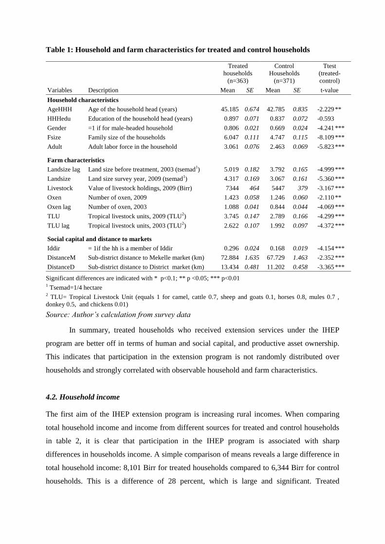
Table 1: Household and farm characteristics for treated and control households

Treated

households

(n=363)

Control

Households

(n=371)

Ttest

(treated-

control)

Variables Description Mean SE Mean SE t-value

Household characteristics

AgeHHH Age of the household head (years) 45.185 0.674 42.785 0.835 -2.229 **

HHHedu Education of the household head (years) 0.897 0.071 0.837 0.072 -0.593

Gender =1 if for male-headed household 0.806 0.021 0.669 0.024 -4.241 ***

Fsize Family size of the households 6.047 0.111 4.747 0.115 -8.109 ***

Adult Adult labor force in the household 3.061 0.076 2.463 0.069 -5.823 ***

Farm characteristics

Landsize lag Land size before treatment, 2003 (tsemad1) 5.019 0.182 3.792 0.165 -4.999 ***

Landsize Land size survey year, 2009 (tsemad1) 4.317 0.169 3.067 0.161 -5.360 ***

Livestock Value of livestock holdings, 2009 (Birr) 7344 464 5447 379 -3.167 ***

Oxen Number of oxen, 2009 1.423 0.058 1.246 0.060 -2.110 **

Oxen lag Number of oxen, 2003 1.088 0.041 0.844 0.044 -4.069 ***

TLU Tropical livestock units, 2009 (TLU2) 3.745 0.147 2.789 0.166 -4.299 ***

TLU lag Tropical livestock units, 2003 (TLU2) 2.622 0.107 1.992 0.097 -4.372 ***

Social capital and distance to markets

Iddir = 1if the hh is a member of Iddir 0.296 0.024 0.168 0.019 -4.154 ***

DistanceM Sub-district distance to Mekelle market (km) 72.884 1.635 67.729 1.463 -2.352 ***

DistanceD Sub-district distance to District market (km) 13.434 0.481 11.202 0.458 -3.365 ***

Significant differences are indicated with * p<0.1; ** p <0.05; *** p<0.01 1 Tsemad=1/4 hectare

2 TLU= Tropical Livestock Unit (equals 1 for camel, cattle 0.7, sheep and goats 0.1, horses 0.8, mules 0.7 ,

donkey 0.5, and chickens 0.01)

Source: Author’s calculation from survey data

In summary, treated households who received extension services under the IHEP

program are better off in terms of human and social capital, and productive asset ownership.

This indicates that participation in the extension program is not randomly distributed over

households and strongly correlated with observable household and farm characteristics.

4.2. Household income

The first aim of the IHEP extension program is increasing rural incomes. When comparing

total household income and income from different sources for treated and control households

in table 2, it is clear that participation in the IHEP program is associated with sharp

differences in households income. A simple comparison of means reveals a large difference in

total household income: 8,101 Birr for treated households compared to 6,344 Birr for control

households. This is a difference of 28 percent, which is large and significant. Treated

households have larger incomes than control households but given the non-random

distribution of the program this does not say anything about the impact of the IHEP extension

program. Further in-depth econometric analysis is needed to address causality.

Table 2: Income and income sources for treated and control households

Treated

households

(n=363)

Control

households

(n=371)

ttest

(treated-

control)

Mean SE Mean SE t-value

Total average income

Total household income

8,101 420 6,344 323 -3.327 ***

Average income from different sources1

Farm income

5,546 305 4,306 305 -2.872 ***

Income from cropping

4,659 299 3,752 301 -2.139 **

Income from livestock-rearing 887 78 554 47 -3.646 ***

Non-farm income 2,375 287 1,455 98 -3.058 ***

Income from wages 1,725 156 1,115 67 -3.612 ***

Income from non-farm businesses

650 169 340 70 -1.710 **

Non-labor income 180 41 583 99 3.724 ***

Transfer income2

37 11 215 58 2.989 ***

Migration income3 142 40 368 78 2.573 ***

Average share of income from different sources

Farm income 68.5 67.9

Non-farm income 29.3 22.9

Non-labor income 2.2 9.2

Income diversification

Income diversification index (SID)4

0.428 0.011 0.419 0.011 -0.551

Significant differences are indicated with * p<0.1; ** p <0.05; *** p<0.01 1 Income from all different sources are calculated for the 12 months period prior to the survey.

2 Transfer income refers to public transfers from governmental and non-governmental programs (in cash or in

kind). 3 Migration income refers to remittances sent by migrated household and family members.

4 The Simpson index of diversity (SID) is defined as

; Where is the proportion of income

coming from source


Farming is the most important activity in the region, and both treated and control

households obtain on average about 70 percent of their total household income from farming

(table 2). Crop income is the most important part of farm income and is significantly higher

for treated households (4,659 Birr) than for control households (3,752 Birr). Also the

difference in livestock income between treated and control households are significant: 887

Birr and 554 Birr for treated and control households respectively. Non-farm income,

including income from wages7 as well as income from non-farm businesses, accounts for

about 25 percent of total income for both groups and is again significantly higher for treated

households (2,375 Birr) than for control households (1,455 Birr). The superior performance of

treated households in terms of farm and non-farm income is in line with what one would

expect given the better capital and asset position of these households. From the presented

descriptive statistics it remains unclear whether the observed differences in income are

attributable to the impact of the extension program or to differences in the underlying

characteristics of treated versus control households.

Non-labor income is more important in the income portfolio of control households,

where it amounts to 9.2 percent of total household income (compared to 2.2 percent for

treated households). The largest share of non-labor income comes from public transfers in the

form of food aid. This could indicate that control households are poorer and more often need

to rely on government and charity aid.

4.3. Income diversification

The second aim of the IHEP extension program is to diversify rural incomes away from

agriculture and cropping. To compare the degree of income diversification between treated

and control households the Simpson Index of Diversification (SID) was calculated. This index

is calculated as follows:

(1)

with Vi the proportion of income from source i. The value of SID is low when households

have few different income sources and becomes 0 when the household depends on only one

income source. The value increases with the number of different income sources and

approaches one if the number of income sources becomes very large (Minot et al, 2006). The

index is in line with a definition of income diversification referring to an increase in the

number of income sources and the balance among them8 (Joshi et al., 2003; Minot et al.,

7 An important part of wage income comes from employment in public safety net employment programs,

designed to provide households with enough income (cash/food) to meet their food gap and protect their assets

during crises periods. 8 This is the most common used definition of income diversification. Others have used other notions of income

diversification: e.g. as a switch from subsistence food production to commercial agriculture (Delgado and

Siamwalla, 1997); as expansion in the importance of non-crop or non-farm income (Reardon, 1997); or as a

switch from low-value crop production to high-value crops, livestock and non-farm activities (Minot et al.,

2006).

2006; Dercon, 1998). To calculate the index, we took into account six income sources:

cropping, livestock rearing, wages, non-farm business, public transfers and private transfers.

This diversification index is reported in table 2. The index is slightly higher for treated

households (0.428) than for control households (0.419) but the difference is very small and

statistically not significant. This indicates there is no difference in the degree of income

portfolio diversification between households receiving extension services and households not

receiving those services.

Table 3: Income and income sources across income diversification quintiles

Income diversification (SID) quintiles, from

lowest (1) to highest (5) diversification

1 2 3 4 5

Total income 9,910 6,528 6,147 6,678 6,846

Farm income 8,772 4,866 3,726 3,882 3,408

Income from cropping 8,546 4,418 3,121 2,983 1,997

Income from livestock- rearing 226 448 605 899 1,411

Non-farm income 1,115 1,328 2,000 2,327 2,770

Income from wages 769 917 1,609 1,929 1,853

Income from non-farm businesses 346 411 392 398 917

Non-labor income 23 334 420 469 667

Transfer income2 19 87 153 75 301

Migration income3 4 247 266 394 367

1 The Simpson index of diversity (SID) is defined as

; Where is the proportion of income

coming from source 2 Transfer income refers to public transfers from governmental and non-governmental programs (in cash or in

kind). 3 Migration income refers to remittances sent by migrated household and family members.

Source: Authors ‘calculation from survey data

In the literature, there is a debate on the relation between income levels and income

diversification. Some authors argue that diversification of incomes away from farm activities

lead to higher income levels but that households face constraints to enter such new non-farm

income-generating activities (Dercon, 1998; Woldenhanna and Oskam, 2001; Barrett et al.,

2001a). Others argue that income diversification is associated with lower incomes because

households choose to diversify their activities at a cost of lower return as a risk coping

mechanism (Barrett et al., 2001b; Ellis, 1998). To shed more light on the relation between

income and income diversification in our case study, we classified our sampled households in

income diversification quintiles and compare incomes across the quintiles (table 3). This

reveals that households with the least diversified incomes have the highest total incomes and

are specialized in cropping. The lowest average income is found among households in the

middle income diversification quintile. The households in the highest income diversification

quintiles have the lowest cropping incomes but the highest incomes from livestock rearing,

wage employment, non-farm business activities, and transfers. This indicates that income and

income diversification are negatively correlated at lower levels of income diversification and

positively correlated at higher levels of income diversification.

4.4. Investment and expenditures

In addition to income measures of welfare, we also consider investment and expenditures

measures and compare them across treated and control households in table 4. We find that

treated households invested more in livestock (2,640 Birr) than control households (1,336

Birr) but that their overall asset formation is not significantly different from that of control

households. This could be expected, as some packages of the IHEP extension program

specifically focus on livestock rearing (dairy, poultry, sheep and goats) and improved animal

breeds.

Table 4: Investment and expenditures for treated and control households

Treated

households

(n= 363)

Control

households

(n=371)

ttest (treated-

control)

Mean SE Mean SE t-value

Fixed asset formation a

12,765 1,110 10,556 1,541 -1.159

Livestock investment b

2,640 203 1,336 136 -5.339 ***

Significant differences are indicated with * p<0.1; ** p <0.05; *** p<0.01 a

Fixed asset formation includes households’ investment during the 12 months prior the survey in houses,

agricultural equipment, consumer durables (furniture, electronic appliances, etc), valued at the survey year price

level. b

Livestock investment includes households’ investment in the different livestock units (cattle, beehives, poultry,

etc) during 12 months prior to the survey, valued at the survey year price level.


5. Econometric analysis of welfare effects

The descriptive analysis presented in the previous section shows that there are substantial

differences in the underlying characteristics of treated versus control households as well as in

their incomes and investment. However, based on a simple comparison of means it is

impossible to identify causality and to attribute the observed differences in welfare outcomes

to the impact of the extension program. In this section we present an econometric analysis to

estimate the causal impact of participation in the IHEP extension program on household

income, income diversification, and investment.

5.1. Estimation approach

Participation in the IHEP extension service is not random and strongly correlated with

observable household and farm characteristics. This complicates the estimation of the causal

impact of the program and gives rise to selection bias. This may arise from households’ self-

selection into the extension program or from endogenous program placement. Households

may decide, based on their access to productive resources, to participate in the extension

services and self-select into the program. In addition, program administrators and extension

agents may target certain villages and select households with specific characteristics.

We address the potential selection problem using propensity score matching and

regression techniques. These are state-of-the-art methods proposed in program evaluation

(Imbens, 2004; Wooldridge, 2008) and increasingly applied in the empirical agricultural

economics literature (e.g. Maertens and Swinnen, 2009; Imai et al., 2010; Becerril and

Abdulai, 2009; Faltermeier and Abdulai, 2009). First, we use a regression model – referred to

as regression on covariates – in which we control for selection bias by including a large set of

observable covariates. The model is specified as follows:

(2)

The variable T is the treatment variable, a dummy variable specifying whether or not the

household has participated in the IHEP extension program. The causal effect of the extension

program, or the treatment effect, is estimated by the coefficient β1. Different outcome

variables Y are considered: 1/ total household income; 2/ livestock investments; 3/ fixed asset

formation; and 4/ income diversification (SID). The outcome variables are measured and

calculated as explained in section 4 and are, except for the diversification index, specified in

logarithmic terms. The vector X1 is a vector of control variables, including the age of the

household head (ageHHH), household head education (HHHedu), household head gender

(Gender), adult labor force (Adult), initial 2003 landholdings (Landsize_lag), initial 2003

livestock holdings (TLU_lag), initial 2003 number of oxen owned (Oxen_lag), Iddir

membership (Iddir), distance to main market (DistanceM) and distance to local market

(DistanceD). The lagged variables for 2003 refer to a base year, before the IHEP program

started. By including a large set of control variables, we account for the observed

heterogeneity across treated and control households.

Second, we estimate a propensity score and use this as an additional control variables

in the regression model. We refer to this model as regression on the propensity score. The

model is specified as follows:

(3)

with T, X1 and Y as defined above in equation (3.2) and the coefficient β1 being the treatment

effect of interest. The variable PS is the propensity score or the estimated conditional

probability of being treated. Adding the propensity score as an additional control variable in

the regression further reduces the potential bias created by selection on observable

characteristics (Imbens, 2004). The propensity score is estimated as the probability of

receiving extension services using a probit model:

(4)

Third, we estimate the treatment effect using different propensity-score matching

techniques, which we refer to as matching on the propensity score. This method involves

matching treated households with control households that are similar in terms of observable

characteristics (Imbens, 2004; Imbens and Angrist; 1995; Caliendo and Kopeinig, 2008). As

matching directly on observable characteristics is difficult if the set of potentially relevant

characteristics is large, matching on propensity scores has been proposed as a valid method

(Rosenbaum and Rubin, 1983). We match every treated household in our sample with one or

several control households with a similar propensity score, using the propensity score as

estimated in equation (3.4) and using different matching methods. We first use stratification

matching, which involves the identification of strata with different ranges of the propensity

score. We then apply single-nearest neighbor matching, in which every treated household is

matched to the control household with the closest propensity score. According to Imbens

(2004) this leads to the most credible inferences with the least bias. This can however result in

poor matches if the difference in the propensity score between the treated and the closest

control unit is still large. We therefore additionally apply radius matching with a caliper

distance of 0.1 as threshold tolerance level of propensity score distance between treated and

matched controls. We finally apply kernel matching, using the default Gaussian kernel. This

involves matching every treated unit to a construct that is a weighted average of all control

units with weights depending on the propensity score distance between the treated and

controls. The advantage of kernel matching is that all information from all control units is

used. Since the sub-sample of control observations is relatively small, matching is always

done with replacement. As propensity score matching methods are sensitive to the exact

specification and matching method, the use of different matching techniques serves as a

robustness check.

After matching treated households with control households on the propensity score,

the average treatment effect of the treated (ATT) is calculated as a weighted difference

between treated and matched controls. The ATT measures the impact of the extension

program for households participating in the program and is calculated as follows:

Cj

C

i

Ti

T

i

T

YjiYN

),(1

(5)

with NT the number of treated observations, YT outcome with treatment, Y

C outcome without

treatment, and ω(i,j) the weight factor used in matching. The latter factor is 1 in case of single

nearest neighbor matching and smaller than 1 in case of radius and kernel matching. We

estimate the ATT using propensity score matching for all four outcome variables of interest:

1/ total household income; 2/ livestock investments; 3/ fixed asset formation; and 4/ income

diversification.

The reliability of propensity score matching estimators depends on two crucial

assumptions. First, the conditional independence assumption requires that given observable

variables, potential outcomes are independent of treatment assignment (Imbens, 2004)9. This

implies that selection into treatment is based entirely on observable covariates, which is a

strong assumption. Second, the common support or overlap condition requires that treatment

observations have comparison control observations nearby in the propensity score distribution

(Caliendo and Kopeinig, 2008). As proposed by Heckman et al. (1997) only observations in

the common support region – where the propensity score of the control units is not smaller

than the minimum propensity score of the treated units and the propensity score of the treated

units not larger than the maximum propensity score of the control units – are used in the

9 This assumption is also referred to as unconfoundedness (Rosenbaum and Rubin, 1983), selection on

observables (Heckman and Robb, 1985)

analysis. This comes down to dropping ten control observations for which the estimated

propensity score is higher than the maximum propensity score of the treated units. The two

assumptions are further addressed in section 5.3 after the discussion of the results.

5.2. Results and discussion

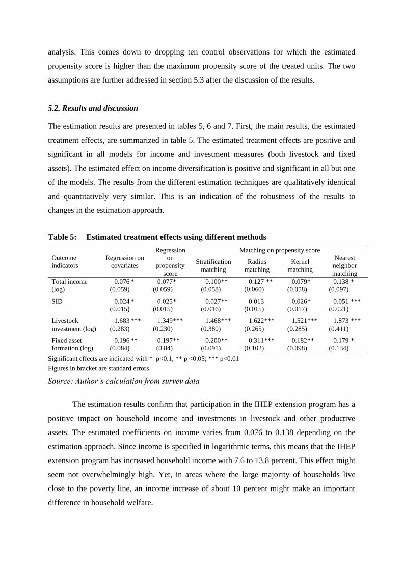
The estimation results are presented in tables 5, 6 and 7. First, the main results, the estimated

treatment effects, are summarized in table 5. The estimated treatment effects are positive and

significant in all models for income and investment measures (both livestock and fixed

assets). The estimated effect on income diversification is positive and significant in all but one

of the models. The results from the different estimation techniques are qualitatively identical

and quantitatively very similar. This is an indication of the robustness of the results to

changes in the estimation approach.

Table 5: Estimated treatment effects using different methods

Outcome

indicators

Regression on

covariates

Regression

on

propensity

score

Matching on propensity score

Stratification

matching

Radius

matching

Kernel

matching

Nearest

neighbor

matching

Total income

(log)

0.076 * 0.077 * 0.100 ** 0.127 ** 0.079 * 0.138 *

(0.059) (0.059) (0.058) (0.060) (0.058) (0.097)

SID 0.024 * 0.025 * 0.027 ** 0.013 0.026 * 0.051 ***

(0.015) (0.015) (0.016) (0.015) (0.017) (0.021)

Livestock

investment (log)

1.683 *** 1.349 *** 1.468 *** 1.622 *** 1.521 *** 1.873 ***

(0.283) (0.230) (0.380) (0.265) (0.285) (0.411)

Fixed asset

formation (log)

0.196 ** 0.197 ** 0.200 ** 0.311 *** 0.182 ** 0.179 *

(0.084) (0.84) (0.091) (0.102) (0.098) (0.134)

Significant effects are indicated with * p<0.1; ** p <0.05; *** p<0.01

Figures in bracket are standard errors


The estimation results confirm that participation in the IHEP extension program has a

positive impact on household income and investments in livestock and other productive

assets. The estimated coefficients on income varies from 0.076 to 0.138 depending on the

estimation approach. Since income is specified in logarithmic terms, this means that the IHEP

extension program has increased household income with 7.6 to 13.8 percent. This effect might

seem not overwhelmingly high. Yet, in areas where the large majority of households live

close to the poverty line, an income increase of about 10 percent might make an important

difference in household welfare.

The estimated effect on investment is much higher. For investment in livestock the

estimated coefficients ranges from 1.87 to 1.34 depending on the estimation approach, and for

overall asset investment from 0.19 to 0.31. Given the logarithmic specification, this indicates

that the IHEP extension program more than doubled investment in livestock and increased

overall asset investment with 20 to 30 percent. These are very large and important effects. In

view of the nature of the program with a large focus on dairy, sheep and goats, the high

effects on livestock investment are not surprising. The high impact of the program on

productive investment might create additional long term benefits in terms of future growth in

income and improved household resilience to risk and shocks.

We find a positive effect of the extension program on income diversification. This

effect is not significant in the radius matching estimation but is significant at the 10% or 5%

level for the other estimations. Given that the SID index ranges from 0 to 0.73 in the sample

and that the average is 0.42, the estimated effect is relatively small, ranging from 0.013 to

0.051. We can take this as an indication that het program had a positive but small effect on

income diversification. The IHEP program also focused on non-cropping and non-farm

activities and income diversification was a specific goal of the program. In this respect, the

small effect is somewhat surprising and might indicate that non-farm activities received less

attention in the program, either from the extension agents or from the beneficiary households

themselves. Our findings corroborate the scarce empirical evidence in the literature on the

impact of contemporary extension programs in Ethiopia. Our results are in line with the

results of Dercon et al. (2009) who showed that public extension programs reduced poverty

with 9.8 percent and increased household consumption with 7.1 percent.

Second, the results of the full regression models are presented in table 6. These results

reveal that apart from participation in the IHEP extension program, other variables determine

household income, investment and income diversification. Older households are found to

have lower levels of income and income diversification. Male-headed households have

incomes that are 29 percentage points higher than female-headed households, have more

diversified incomes and make larger investments in livestock. As could be expected, access to

productive resources increases household income. More labor, larger initial landholdings and

larger initial livestock holdings have a significant positive impact on income. Households

with initially more land invest less in livestock and have less diversified income portfolios

while households with initially larger livestock holdings invest even more in livestock and

other assets. Social capital, measured by membership of an Iddir organization, has a positive

and significant impact on income and investment. Distance to the main market has a negative

impact on income, investment and income diversification.

Table 6: Regression results for different outcome indicators

Outcome indicators

Covariates Total income

(log) SID

Livestock

investment (log)

Fixed asset

formation (log)

Treatment 0.076* .024* 1.8683*** 0.196**

(0.059) (0.015) (0.283) (0.084)

AgeHHH -0.010*** -.003*** -0.006 0.001

(0.002) (0.001) (0.011) (0.003)

HHHedu 0.020 -.005 0.215** 0.018

(0.023) (0.006) (0.011) (0.033)

Gender 0.292*** 0.030* 0.939*** 0.044

(0.074) (0.020) (0.354) (0.105)

Adult 0.104*** 0.015*** 0.146* 0.107***

(0.023) (0.006) (0.110) (0.032)

Landsize_lag 0.036*** -0.011*** -0.176*** 0.038**

(0.012) (0.003) (0.057) (0.018)

TLU_lag 0.070*** -0.009** 0.350*** 0.109***

(0.017) (0.004) (0.083) (0.024)

Oxen_lag 0.151*** 0.033*** -0.050 0.215***

(0.041) (0.010) (0.195) (0.058)

Iddir 0.206*** 0.019 0.916*** 0.173*

(0.076) (0.020) (0.364) (0.108)

DistanceM -0.004*** -0.000 -0.021*** -0.009***

(0.001) (0.000) (0.006) (0.001)

DistanceD 0.006** -0.005*** -0.041*** -0.007

(0.003) (0.001) (0.018) (0.005)

Constant 8.194*** 0.589*** 3.674*** 8.191***

(0.168) (0.044) (0.805) (0.240)

# of observations 730 730 730 730

R2

0.28 0.10 0.17 0.21

Adj R2 0.27 0.09 0.16 0.20

F(11,718) 25.00 7.19 13.35 17.66

Prob>F 0.000 0.000 0.000 0.000


Figures in bracket are standard errors


Third, table 7 gives the results of the probit model estimating the propensity score.

The model is statistically significant at the 1 percent level and correctly predicts 64 percent of

the observations. We observe that farmers’ education and household labor resources

positively affect participation in the extension program. This is in line with previous studies

on extension services (e.g. Chianu and Tsujii, 2004; D’Souza et al., 1993). This indicates that

labor constraints might exist for participating in extension services that promote new

technologies and activities that might be labor and skill intensive. The results indicate that

initial landholdings have a positive impact on the probability of participating in the extension

program but initial livestock holdings have no effect. This is not completely in line with the

IHEP program strategy to target poorer and less-endowed households and might indicate there

is still a bias towards households with larger farms in program placement.

Tables 7: Estimation of the propensity score

Covariates Marginal effects SE

AgeHHH 0 .001 .001

HHHedu 0 .028** .016

Gender 0 .034 .050

Adult 0 .065*** .015

Landsize_lag 0 .014** .008

TLU_lag 0 .004 .012

Oxen_lag 0 .006 .027

Iddir 0 .184*** .049

DistanceM 0 .002*** .001

DistanceD 0 .006** .002

Log Likelihood -461.84

LR Chi2 (11) 88.22

Prob > chi2 0.000

Pseudo R2 0.09

% correctly predicted 63.84



Distance to markets, both local and urban markets, is found to positively affect

participation in the extension program. This contradicts most findings from previous studies

(e.g. Mendola, 2007; Gebremedhin et al., 2009), but similar results were found by Genius et

al. (2006). This finding might be related to the fact that the IHEP program aims at a poverty

outreach and specifically targets remote areas where poverty headcount ratios are higher.

Further, we find that membership in an Iddir, a measure of social capital, has a positive effect

on the likelihood of participating in an extension program. This result indicates that social

capital is important for access to programs and is in line with other studies (e.g. Tiwari et al.,

2008; Zepeda, 1990).

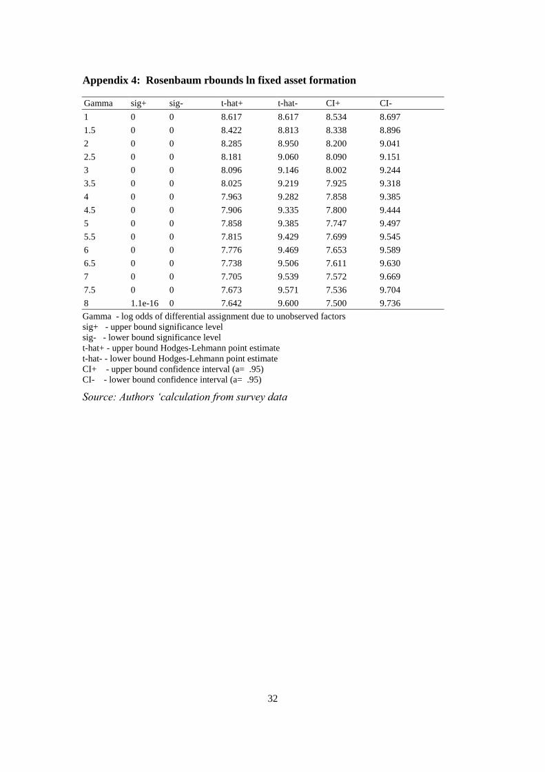
5.3. Assumptions

First, the conditional independence (CI) assumption is intrinsically not testable because the

data are completely uninformative about the distribution of the treated outcome for untreated

observations and vice versa (Imbens, 2004; Becker and Ichino and, 2002). Yet, we can check

the sensitivity of our estimations to deviations from the CI assumption. We do so by using an

approach first proposed by Rosenbaum (2002) and discussed in detail by Becker and Caliendo

(2007). We perform this test using the rbounds command in stata (Becker and Caliendo,

2007) and report the results in appendix 3.1 to 3.4. The sensitivity analysis indicates that for

all outcome variables (income, income diversification, livestock investment and fixed asset

formation) the estimated ATTs are insensitive to a bias that would eightfold the odds of

treatment due to unobserved effects. This implies that our matching estimates are free of bias

caused by unobserved factors.

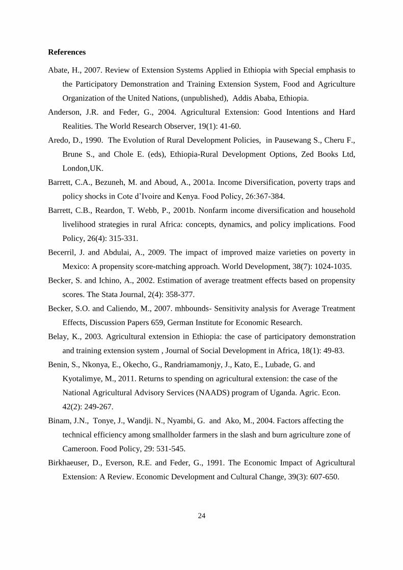
Figure 1: Distribution of the estimated propensity scores over treated and control

households

Source: Author’s estimation from survey data

Second, we verify the common support condition by comparing the propensity score

distribution of the treated and control observations. This is done in figure 3.1. The figure

.2.4

.6.8

1

Control Treatment

Pro

pe

nsity

Score

(P

ropa

bili

ty T

reatm

en

t=1)

Graphs by Extension Partcipation Status

shows that the propensity scores are strictly between 0 and 1, which is a first requirement

(Imbens, 2004), and that there is sufficient overlap in the propensity scores of treated and

control units with a large region of common support.

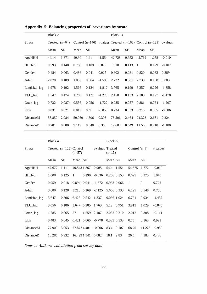
Third, we test the balancing properties for all covariates in the identified strata of

propensity score ranges. These balancing properties are reported in appendix 3.5. The results

indicate that all covariates are balanced in all strata at the 1% level. From this, we can

conclude that the there is sufficient balance in the covariate distribution between treated the

treated and matched control group.

6. Conclusion

This study examined the impact the IHEP extension program in the Tigray region in Ethiopia.

Since this program concerns a new extension approach that is moving towards a more

decentralized, integrated and participatory system, understanding the impact on local farm

households is important. We find that the program importantly contributed to rising household

income and investment in the region. Effects on income diversification were small. We can

conclude that the IHEP program had an important positive welfare impact and extending the

program further to reach the majority of rural households in the Tigray region will likely

benefit the welfare of rural households further.

24

References

Abate, H., 2007. Review of Extension Systems Applied in Ethiopia with Special emphasis to

the Participatory Demonstration and Training Extension System, Food and Agriculture

Organization of the United Nations, (unpublished), Addis Ababa, Ethiopia.

Anderson, J.R. and Feder, G., 2004. Agricultural Extension: Good Intentions and Hard

Realities. The World Research Observer, 19(1): 41-60.

Aredo, D., 1990. The Evolution of Rural Development Policies, in Pausewang S., Cheru F.,

Brune S., and Chole E. (eds), Ethiopia-Rural Development Options, Zed Books Ltd,

London,UK.

Barrett, C.A., Bezuneh, M. and Aboud, A., 2001a. Income Diversification, poverty traps and

policy shocks in Cote d’Ivoire and Kenya. Food Policy, 26:367-384.

Barrett, C.B., Reardon, T. Webb, P., 2001b. Nonfarm income diversification and household

livelihood strategies in rural Africa: concepts, dynamics, and policy implications. Food

Policy, 26(4): 315-331.

Becerril, J. and Abdulai, A., 2009. The impact of improved maize varieties on poverty in

Mexico: A propensity score-matching approach. World Development, 38(7): 1024-1035.

Becker, S. and Ichino, A., 2002. Estimation of average treatment effects based on propensity

scores. The Stata Journal, 2(4): 358-377.

Becker, S.O. and Caliendo, M., 2007. mhbounds- Sensitivity analysis for Average Treatment

Effects, Discussion Papers 659, German Institute for Economic Research.

Belay, K., 2003. Agricultural extension in Ethiopia: the case of participatory demonstration

and training extension system , Journal of Social Development in Africa, 18(1): 49-83.

Benin, S., Nkonya, E., Okecho, G., Randriamamonjy, J., Kato, E., Lubade, G. and

Kyotalimye, M., 2011. Returns to spending on agricultural extension: the case of the

National Agricultural Advisory Services (NAADS) program of Uganda. Agric. Econ.

42(2): 249-267.

Binam, J.N., Tonye, J., Wandji. N., Nyambi, G. and Ako, M., 2004. Factors affecting the

technical efficiency among smallholder farmers in the slash and burn agriculture zone of

Cameroon. Food Policy, 29: 531-545.

Birkhaeuser, D., Everson, R.E. and Feder, G., 1991. The Economic Impact of Agricultural

Extension: A Review. Economic Development and Cultural Change, 39(3): 607-650.

25

Caliendo, M. and Kopeinig, S., 2008. Some practical guidance for the implementation of

propensity score matching, Journal of Economic Surveys, 22(1): 31-72.

Central Statistical Agency, 2007. The 2007 National Statistics, Addis Ababa, Ethiopia.

Chianu, J.N. and Tsujii, H., 2004. Determinants of farmers’ decision to adopt or not adopt

inorganic fertilizer in the savannas of northern Nigeria, Nutrient Cycling in

Agroecosystems 70:293-301.

Cunguara, B., and Moder, K. 2011. Is agricultural extension helping the poor? Evidence from

rural Mozambique. Journal of African Economies 20(4): 562-595.

Delgado, C.L and Siamwalla, A., 1997. Rural Economy and Farm Income Diversification in

Developing Coutries, Discussion paper No. 20, Markets and Structural Studies Division,

IFPRI, Washington, D.C..

D’Souza, G., Cyphers, D. and Phipps, T., 1993. Factors Affecting the Adoption of Sustainable

Agricultural Practices. Agricultural and Resource Economics Review 22:159-165.

Dercon, S., 1998. Wealth, risk and activity choice: cattle in western Tanzania. Journal of

Development Economics 55(1): 1-42.

Dercon, S., Gilligan, D. O., Hoddinott, J. and Woldenhanna, T., 2009. The Impact of

Agricultural Extension and Roads on Poverty and Consumption Growth in Fifteen

Ethiopian Villages. American Journal Agricultural Economics, 91(4): 1007-1021.

Diao, X., 2010. Economic Importance of Agriculture for Sustainable Development and

Poverty Reduction: The Case-Study of Ethiopia. Paper presented at the Global Forum on

Agriculture, 29-30 November 2010, OECD, Paris.

Dinar, A., 1996. Extension Commercialization: How much to charge for extension services.

American Journal of Agricultural Economics, 78(1): 1-12

Ellis, F., 1998. Household Strategies and Rural Livelihood Diversification: Survey article,

The Journal of Development Studies, 35(1): 1-38.

Evenson, R.E., 2001. Economic Impacts of Agricultural Research and Extension, In:

Gardener B.L. and Rausser G.C. (Eds) Handbook of Agricultural Economics Volume 1A

Agricultural Production, Elsevier.

Faltermeier, L. and Abdulai, A., 2009. The impact of water conservation and intensification

technologies: empirical evidence for rice farmers in Ghana, Agricultural Economics,

40:365-379.

Feder, G., Just, R.E., Zilberman, D., 1985. Adoption of agricultural innovations in developing

countries: A survey, Economic Development and Cultural Change, 33(2): 255-298.

26

Feder, G., Murgai, R., and Quizon, J.B., 2004. Sending farmers back to school: The impact of

farmer field schools in Indonesia. Review of Agricultural Economics, 26(1): 45-62.

Gebremedhin, B., Hoekstra, D. and Tegegne, A., 2006. Commercialization of Ethiopian

agriculture: extension service from input supplier to knowledge broker and facilitator.

IPMS (Improving Productivity and Market Success) of Ethiopian farmers project, ILRI

(International Livestock Research Institute), Working Paper No. 1;

Gebremedhin, B., Jaleta. M., and Hoekstra, D., 2009. Smallholders, institutional services, and

commercial transformation in Ethiopia. Agricultural Economics, 40:773-787.

Genius, M.G., Pantzios, C.J., and Tzouvelekas, V., 2006. Information Acquisition and

Adoption of Organic Farming Practices. Journal of Agricultural and Resource

Economics, 31(1): 93-113.

Haji, J., 2006. Production Efficiency of Smallholders’ Vegetable-dominated Mixed Farming

System in Eastern Ethiopia: A Non-Parametric Approach. Journal of African Economies,

16(1):1-27.

Heckman, J., Ichimura, H, and Todd, P. 1997. Matching as an econometric evaluation

estimator: evidence from evaluation a job training program. Review of Economic Studies,

64(4): 605-654.

Heckman, J.J. and Robb, R., 1985. Alternative models for evaluating the impact of

interventions. An overview. Journal of Econometrics 30: 239-267.

Imai, K.S., Arun, T. and Annim, S. K., 2010. Microfinance and Household Poverty

Reduction: New Evidence from India, World Development, 38(12): 1760-1774.

Imbens, G., 2004. Nonparametric estimation of Average Treatment Effects Under

Exogeneity: A Review, The Review of Economics and Statistics; 86(1): 4-29.

Imbens, G.W. and Angrist, J.D., 1995. Two-Stage Least Squares Estimation of Average

Causal Effects in Models With Variable Treatment Intensity, Journal of the American

Statistical Association, 90(430):431-442.

Joshi, P. K., Gulati, A., Birthal, P.S., and Tewari, L., 2003. Agriculture diversification in

south Asia: Pattern, determinants and policy implications, Washington, DC: IFPRI

MSSD Discussion Paper No. 57.

Leeuwis, C. 2003. Communication for Rural Innovation: Rethinking Agricultural Extension.

Blackwell Publishing, UK.

27

Maertens, M. and Swinnen, J.F.M., 2009. Trade, Standards, and Poverty: Evidence from

Senegal, World Development; 37(1): 161-179.

Mendola, M., 2007. Agricultural Technology Adoption and Poverty Reduction: A propensity

–score matching analysis for rural Bangladesh, Food Policy 32: 372-393.

Minot, N., Epprecht, M., Anh, T., Trung, L.Q., 2006. Income Diversification and Poverty in

the Northern Uplands of Vietnam, Research Report 145, International Food Policy

Research Institute, Washington, DC.

Pender, J., F. Place, and S. Ehui, eds. 2006. Strategies for sustainable land management in the

East African highlands.Washington, D.C. International Food Policy Research Institute.

Reardon, T., 1997. Using evidence of household income diversification to inform study of the

rural non-farm labor market in Africa, World Development 25(5): 735-48.

Rivera, W.M., 1997. Decentralizing agricultural extension: alternative strategies, International

Journal of Lifelong Education, 16(5): 393-407.

Rivera, W.M., 2001. Agricultural and Rural Extension Worldwide: Options for Institutional

Reform in the Developing Countries. Food and Agricultural Organization, Rome.

Rosenbaum, P. and Robin, D., 1983. The central role of the propensity score in observational

studies for causal effects. Biometrika 70(1): 41-50.

Rosenbaum, P.R., 2002. Observational Studies, New York; Springer, 2nd

edition.

Solı´s, D., Bravo-Ureta, B.E. and Quiroga, R.E., 2008. Technical Efficiency among Peasant

Farmers Participating in Natural Resource Management Programmes in Central

America, Journal of Agricultural Economics, 60 (1): 202–219.

Spielman, D.J., Byerlee D., Alemu D. and Kelemework, D., 2010. Policies to promote cereal

intensification in Ethiopia: The search for appropriate public and private roles, Food

Policy, 35: 185-194.

Swanson, B.E., 2008. Global Review of Good Agricultural Extension and Advisory Service

Practices, Food and Agriculture Organization of the United Nations, Rome.

Swinnen, J.F. and Maertens, M., 2007. Globalization, Privatization, and Vertical

Coordination in Food Value Chains in Developing and Transition Countries. Agricultural

Economics 37(2): pp 89-102.

Tigray Bureau of Agriculture and Natural Resource Development-TBoANRD 2003.

Integrated Household Extension Intervention Program in Tigray vol. 1, Mekelle, Tigray,

Ethiopia.

28

Tigray Bureau of Agriculture and Natural Resource Development-TBoANRD. 2004. A study

to identify specialization of areas in agriculture and livestock products (unpublished),

Mekelle, Ethiopia

Tiwari, K.R., Sitaula, B.K., Nyborg, I.L.P., Paudel,G.S., 2008. Determinants of Farmers’

Adoption of Improved Soil Conservation Technology in a Middle Mountain Watershed

of Central Nepal. Environmental Management, 42, 210-222.

Umali-Deininger, D., 1997. Public and Private Agricultural Extension: Partners or Rivals?

The World Bank Research Observer, 12(2): 203-224.

Woldenhanna,T., Oskam. A., 2001. Income diversification and entry barriers: evidence from

the Tigray region of northern Ethiopia, Food Policy 26:351-365.

Wooldridge, J.M., 2008. Introductory Econometrics: A Modern Approach. South-Western

Cengage Learning, Mason, USA.

Zepeda, L. 1990. Predicting Bovine Somatotropine Use by California Dairy Farmers,

Western Journal of Agricultural Economics, 15(1):55-62.

29

Appendix 1: Rosenbaum rbounds for ln household income

Gamma sig+ sig- t-hat+ t-hat- CI+ CI-

1 0 0 8.587 8.587 8.527 8.647

1.5 0 0 8.439 8.730 8.374 8.789

2 0 0 8.331 8.826 8.259 8.886

2.5 0 0 8.243 8.898 8.168 8.959

3 0 0 8.173 8.955 8.091 9.018

3.5 0 0 8.111 9.003 8.026 9.067

4 0 0 8.057 9.043 7.967 9.109

4.5 0 0 8.011 9.078 7.915 9.145

5 0 0 7.968 9.109 7.869 9.178

5.5 0 0 7.928 9.136 7.828 9.208

6 0 0 7.893 9.160 7.788 9.235

6.5 0 0 7.862 9.183 7.750 9.259

7 0 0 7.832 9.205 7.718 9.282

7.5 0 0 7.805 9.224 7.687 9.303

8 1.1e-16 0 7.777 9.242 7.659 9.323

Gamma - log odds of differential assignment due to unobserved factors

sig+ - upper bound significance level

sig- - lower bound significance level

t-hat+ - upper bound Hodges-Lehmann point estimate

t-hat- - lower bound Hodges-Lehmann point estimate

CI+ - upper bound confidence interval (a= .95)

CI- - lower bound confidence interval (a= .95)


30

Appendix 2: Rosenbaum rbounds for income diversification index (SID)


1 0 0 .436 .436 .418 .453

1.5 0 0 .392 .477 .374 .494

2 0 0 .362 .504 .343 .520

2.5 0 0 .340 .523 .322 .538

3 0 0 .323 .537 .304 .553

3.5 0 0 .309 .549 .289 .564

4 0 0 .296 .559 .275 .573

4.5 0 0 .285 .566 .264 .580

5 0 0 .275 .573 .254 .587

5.5 0 0 .267 .578 .247 .593

6 0 0 .259 .584 .239 .599

6.5 0 0 .253 .588 .231 .603

7 0 0 .247 .593 .224 .608

7.5 0 0 .242 .596 .216 .612

8 1.1e-16 0 .237 .600 .210 .615









31

Appendix 3: Rosenbaum rbounds ln livestock investment


1 0 0 4.005 4.005 3.928 4.143

1.5 0 0 3.813 4.294 3.739 4.486

2 0 0 3.661 4.647 3.545 6.978

2.5 0 0 3.504 7.061 3.373 7.334

3 0 0 3.379 7.322 3.239 7.520

3.5 0 0 3.276 7.478 -0.000 7.649

4 0 0 3.155 7.589 -0.000 7.747

4.5 0 0 -0.000 7.675 -0.000 7.827

5 0 0 -0.000 7.747 -0.000 7.894

5.5 0 0 -0.000 7.805 -0.000 7.949

6 3.3e-16 0 -0.000 7.858 -0.000 8.001

6.5 4.3e-15 0 -0.000 7.903 -0.000 8.047

7 3.9e-14 0 -0.000 7.942 -0.000 8.086

7.5 2.6e-13 0 -0.000 7.979 -0.000 8.122

8 1.4e-12 0 -0.000 8.013 -0.000 8.155









32

Appendix 4: Rosenbaum rbounds ln fixed asset formation


1 0 0 8.617 8.617 8.534 8.697

1.5 0 0 8.422 8.813 8.338 8.896

2 0 0 8.285 8.950 8.200 9.041

2.5 0 0 8.181 9.060 8.090 9.151

3 0 0 8.096 9.146 8.002 9.244

3.5 0 0 8.025 9.219 7.925 9.318

4 0 0 7.963 9.282 7.858 9.385

4.5 0 0 7.906 9.335 7.800 9.444

5 0 0 7.858 9.385 7.747 9.497

5.5 0 0 7.815 9.429 7.699 9.545

6 0 0 7.776 9.469 7.653 9.589

6.5 0 0 7.738 9.506 7.611 9.630

7 0 0 7.705 9.539 7.572 9.669

7.5 0 0 7.673 9.571 7.536 9.704

8 1.1e-16 0 7.642 9.600 7.500 9.736









33

Appendix 5: Balancing properties of covariates by strata

Block 2 Block 3

Strata Treated (n=64) Control (n=146) t-values Treated (n=162) Control (n=139) t-values

Mean SE Mean SE Mean SE Mean SE

AgeHHH 44.14 1.871 40.30 1.41 -1.554 42.728 0.952 42.712 1.278 -0.010

HHHedu 0.593 0.140 0.760 0.109 0.879 1.018 0.113 1 0.129 -0.107

Gender 0.484 0.063 0.486 0.041 0.025 0.802 0.031 0.820 0.032 0.389

Adult 2.078 0.109 1.883 0.064 -1.595 2.722 0.881 2.733 0.108 0.083

Landsize_lag 1.978 0.192 1.566 0.124 -1.812 3.765 0.199 3.357 0.226 -1.358

TLU_lag 1.547 0.174 1.269 0.121 -1.275 2.458 0.133 2.183 0.127 -1.478

Oxen_lag 0.732 0.0874 0.556 0.056 -1.722 0.985 0.057 0.881 0.064 -1.207

Iddir 0.031 0.021 0.013 009 -0.853 0.234 0.033 0.215 0.035 -0.386

DistanceM 58.859 2.084 59.959 1.606 0.393 73.506 2.464 74.323 2.681 0.224

DistanceD 8.781 0.680 9.119 0.540 0.363 12.608 0.649 11.550 0.710 -1.100

Block 4 Block 5

Strata Treated (n=122) Control

(n=57)

t-values Treated

(n=15)

Control (n=8) t-values

Mean SE Mean SE Mean SE Mean SE

AgeHHH 47.672 1.111 49.543 1.867 0.905 54.4 1.554 54.375 1.772 -0.010

HHHedu 1.008 0.125 1 0.190 -0.036 0.266 0.153 0.625 0.375 1.048

Gender 0.959 0.018 0.894 0.041 -1.672 0.933 0.066 1 0 0.722

Adult 3.680 0.128 3.210 0.169 -2.125 5.666 0.333 6.125 0.548 0.756

Landsize_lag 5.647 0.306 6.425 0.542 1.337 9.066 1.024 6.781 0.934 -1.457

TLU_lag 3.056 0.186 3.647 0.285 1.763 5.19 0.951 3.913 1.029 -0.845

Oxen_lag 1.285 0.065 57 1.559 2.187 2.053 0.210 2.012 0.308 -0.111

Iddir 0.483 0.045 0.421 0.065 -0.778 0.533 0.133 0.75 0.163 0.991

DistanceM 77.909 3.053 77.877 4.401 -0.006 83.4 9.107 68.75 11.226 -0.980

DistanceD 16.286 0.932 16.429 1.541 0.082 18.1 2.834 20.5 4.183 0.486


Documents

The Economic Impact of a New Rural Extension Approach in Northern Ethiopia