The Effects of Fiscal Shocks on the Exchange Rate in the

Spain§

Francisco de Castro

Banco de España

Laura Fernández

Banco de España

March 2011

Abstract

We analyse the impact of fiscal shocks on the Spanish effective exchange rate over the period

1981-2008 using a standard structural VAR framework. We show that government spending

brings about positive output responses, jointly with real appreciation. Such real appreciation is

explained by persistent nominal appreciation and higher relative prices in the short term,

although the latter fall below baseline values in the medium term. In turn, the current account

deteriorates when government spending rises mainly due to the fall of exports caused by the real

appreciation. Accordingly, our results in this regard are largely consistent not only with the

conventional Mundell-Fleming model and, in general a traditional Keynesian view, but also

with a wide set of RBC or New Keynesian models under standard calibrations. Moreover, our

estimations are fully in line with the “twin deficits” hypothesis. Furthermore, we show that

shocks to purchases of goods and services and public investment lead to real appreciation,

whereas the opposite happens with higher personnel expenditure. We obtain output multipliers

around 0.5 on impact and slightly above unity one year after the shock, which are in line with

previous empirical evidence regarding some individual European countries.

JEL Classification: E62; H30.

Keywords: SVAR; Fiscal Shocks; Effective Exchange Rates; Twin deficits; Fiscal multipliers.

§ The views expressed in this paper are those of the authors and do not necessarily reflect those of the Bank of Spain. Contact details: Francisco de Castro (fcastro@bde.es); Laura Fernández (laurafernandez@bde.es). Directorate General Economics, Statistics and Research. Bank of Spain. C/ Alcalá 48, 28014 Madrid, Spain.

1

1 Introduction

Last years have witnessed an increasing literature on the macroeconomic effects of

discretionary fiscal policy in a wide set of countries. This strand of the literature gained

momentum with Blanchard and Perotti (2002), who proposed a new and interesting

methodology to identify fiscal policy shocks in VARs with quarterly data by exploiting

decision lags in policy making and information about elasticities of fiscal variables to

economic activity.1

However, most of these papers fail to analyse in depth the implications of fiscal

shocks on external competitiveness, a crucial element especially for small open

economies such as Spain. Still, there are some recent studies assessing the effects of

fiscal, mainly spending, shocks on the nominal or real exchange rate, relative prices or

the terms of trade. Nevertheless, as it is commonplace in the analysis of discretionary

fiscal shocks, broad agreement on their effects is lacking. Thus, Kim and Roubini

(2008) and Enders et al. (2011) for the U.S., Monacelli and Perotti (2010) for Australia,

the U.S. and the U.K. and Ravn et al. (2007) for a pool of Australia, Canada, the U.S.

and the U.K., find that higher government expenditure yields real depreciations. By

contrast, Beetsma et al. (2008) for a panel of EU counties, Corsetti et al. (2009) for the

U.S. or Bénétrix and Lane (2009) or Galstyan and Lane (2009) for Ireland argue that

Notwithstanding, other studies such as Mountford and Uhlig (2009)

assess the effects of fiscal shocks under a different methodology that consists in

imposing some sign restrictions to impulse response functions. While most papers have

focused on the U.S. (Edelberg et al, 1999; Fatás and Mihov, 2001; Blanchard and

Perotti, 2002; Perotti, 2004; Mountford and Uhlig, 2009, among others), growing

evidence on other countries has arisen. Some examples in this regard are Heppke-Falk

et al. (2006) for Germany, De Castro (2006) and De Castro and Hernández de Cos

(2008) for Spain, Giordano et al. (2007) for Italy, Marcellino (2006) for the four largest

countries of the euro area or Afonso and Sousa (2009a, 2009b) for Germany, Italy and

Portugal, and Bénassy-Quéré and Cimadomo (2006) for Germany, the U.K. and the

U.S., among others.

1 Perotti (2004) developed this methodology further and has constituted the basis of later studies focused on different countries.

2

government spending shocks lead to real appreciations. In addition, Froot and Rogoff

(1991) and De Gregorio et al., (1994) observe long-run real appreciation in response to

increases in government consumption.

In the related literature real depreciation caused by government expenditure shocks

is justified on the basis of the following argument: in a large economy, a fiscal

expansion increases the real interest rate, which depresses private consumption. Since

the demand for money is assumed to depend on private consumption, insofar as prices

are sticky, a fall in consumption leads to a depreciation of the nominal and real

exchange rate (see Obstfeld and Rogoff, 1995). Moreover, it is also argued that in the

short run international price movements tend to amplify instead of mitigate country-

specific consumption risk (Enders et al, 2010).

Conversely, a usual argument behind spending shocks-led real appreciations is that

insofar as government spending mostly concentrates on home-produced goods, fiscal

expansions should make these goods relatively scarcer, thereby increasing their relative

price with respect to imported goods and leading to real appreciation (see Frenkel and

Razin, 1996).

We aim to provide further evidence in this area by assessing the effects of

government spending shocks on external competitiveness and the current account

balance in Spain. We base our conclusions on impulse response functions drawn from

structural VARs, wherein discretionary fiscal shocks have been identified following the

methodology proposed by Blanchard and Perotti (2002) and Perotti (2004). To our

understanding, this is the first paper that tackles these issues for Spain under this

framework.

We find that government spending shocks lead to real appreciation and

deterioration of the external balance. Hence, our results are in line with the “twin

deficits” hypothesis. The real depreciation is explained by both an appreciation of the

nominal effective exchange rate and by an increase in relative prices. This pattern is

consistent with not only the conventional Mundell-Fleming model and Keynesian

analysis, but also with a wide set of RBC models under standard calibrations or with

some New Keynesian formulations (see, Corsetti et al., 2009).

3

By spending component, we show that shocks to purchases of goods and services

and public investment lead to real appreciation, whereas the opposite happens with

higher personnel expenditure. Finally, we obtain output multipliers around 0.5 on

impact and slightly above unity one year after the shock, which are in line with previous

empirical evidence regarding some individual European countries. However, we offer

interesting evidence of output multipliers being higher if we constraint our estimations

to a period characterised by a quasi-fixed exchange rate regime.

The rest of the paper is organised as follows: section 2 describes the data, section 3

methodological issues and section 4 the results. Finally, we present our conclusions in

section 5.

2 The data

The baseline VAR includes quarterly data on public expenditure (gt), net taxes (tt) and

GDP (yt), all in real terms,2 the GDP deflator (pt), the three-year interest rate of

government bonds (rt)3 and the real effective exchange rate (REER henceforth) vis à vis

the rest of the world. All variables are seasonally adjusted and enter in logs except the

interest rate and the REER, which enter in levels. The definition of fiscal variables

follows Blanchard and Perotti (2002) and Perotti (2004). In particular, government

spending (gt) is defined as the sum of government consumption and investment,

whereas net taxes (tt) are defined as total government current receipts, less current

transfers and interest payments on government debt.4

We try other VAR specifications aiming to better understand the responses of

certain variables to fiscal shocks. For this purpose, we also assessed the reactions of

nominal effective exchange rates, net exports or the role of relative prices. On the other

hand, as we are also interested in the analysis of exchange rate responses to different

In turn, the REER is defined as

usual, namely an increase reflects a real appreciation of the relevant currency.

2 The nominal variables have been deflated by the GDP deflator in order to obtain the corresponding real values. 3 The long-term interest rate is preferred to the short-term one because of its closer relationship with private consumption and investment decisions. However, this choice turned out to be immaterial to the results in that the inclusion of short-term rates in the VAR led to similar conclusions. 4 More concretely, transfers include all expenditure items except public consumption, public investment and interest payments.

4

types of fiscal shocks, we included non-wage government consumption, government

spending on wages and salaries and public investment in turn as endogenous variables.

As before, the GDP deflator was used to get their corresponding real values.

We use data covering the period 1981:Q1 to 2008:Q4. GDP volumes and deflator,

exports, imports and net exports have been taken from the Quarterly National Accounts

(National Institute of Statistics, INE) while the three-year bond rate has been obtained

from the Banco de España database. The quarterly fiscal variables until 2000 were taken

from Estrada et al. (2004), which were estimated applying monthly and quarterly

official fiscal indicators on a cash basis to the official ESA-95 annual account data.

These fiscal variables are the same as those used in De Castro (2006) and De Castro and

Hernández de Cos (2008). However, from 2000 on, those variables are not interpolated;

they are official figures published by the IGAE (Ministry of Economy and Finance).

Finally, real and nominal effective exchange rates have been obtained from the IFS

(IMF) database and are defined in such a way that an increase reflects an appreciation.

Relative prices are computed from the real and the nominal effective exchange rates.

3 Specification and identification of the baseline (S)VAR model

The reduced-form baseline VAR is specified in levels and can be written as

ttt UXLDX += −1)( (1)

where Xt ≡ (gt, tt, yt, pt, rt, reert) is the vector of endogenous variables and D(L) is an

autoregressive lag-polynomial. The benchmark specification includes a constant and a

deterministic time trend. The vector Ut ≡ ( reert

rt

pt

yt

tt

gt uuuuuu , , , , , ) contains the

reduced-form residuals, which in general will present non-zero cross-correlations. The

baseline VAR includes four lags of each endogenous variable according to the

information provided by LR tests, the Akaike information criterion and the final

prediction error.5

5 Schwarz and Hannan-Quinn information criteria suggested more parsimonious specifications. In order to assess the robustness of our results to different specifications and transformations, we tried several alternatives, including estimating with two lags, removing the time trend or substituting the long-term interest rate by a short-term one. These different alternatives showed the same qualitative results.

5

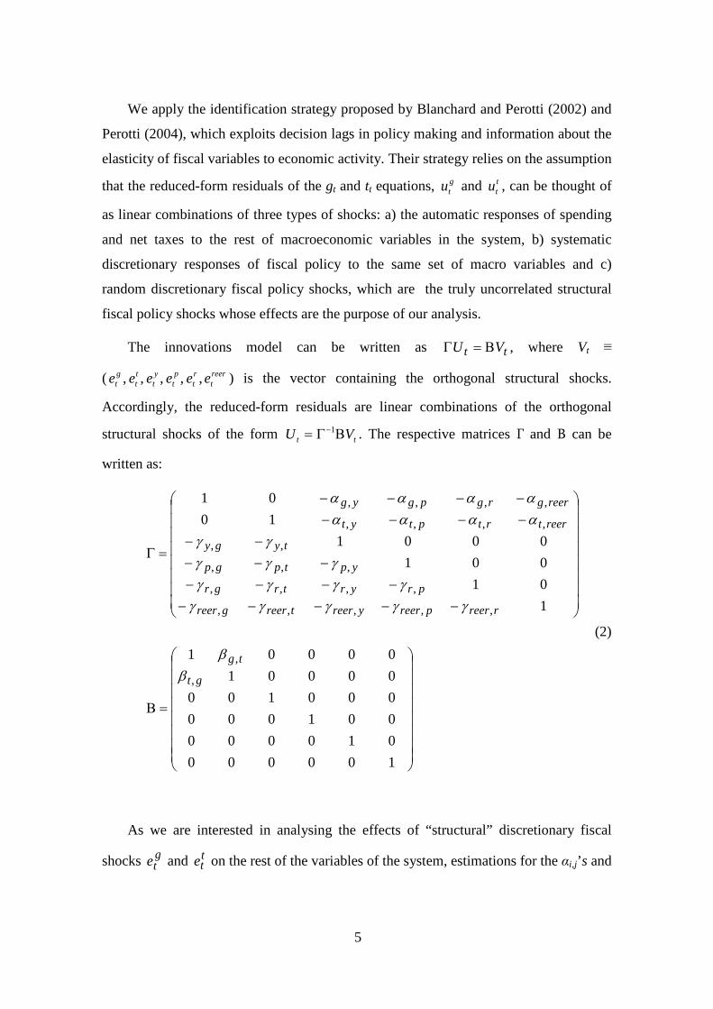
We apply the identification strategy proposed by Blanchard and Perotti (2002) and

Perotti (2004), which exploits decision lags in policy making and information about the

elasticity of fiscal variables to economic activity. Their strategy relies on the assumption

that the reduced-form residuals of the gt and tt equations, gtu and t

tu , can be thought of

as linear combinations of three types of shocks: a) the automatic responses of spending

and net taxes to the rest of macroeconomic variables in the system, b) systematic

discretionary responses of fiscal policy to the same set of macro variables and c)

random discretionary fiscal policy shocks, which are the truly uncorrelated structural

fiscal policy shocks whose effects are the purpose of our analysis.

The innovations model can be written as tt VU Β=Γ , where Vt ≡

( reert

rt

pt

yt

tt

gt eeeeee , , , , , ) is the vector containing the orthogonal structural shocks.

Accordingly, the reduced-form residuals are linear combinations of the orthogonal

structural shocks of the form tt VU ΒΓ= −1 . The respective matrices Γ and Β can be

written as:

=Β

−−−−−−−−−

−−−−−

−−−−−−−−

=Γ

1000000100000010000001000000100001

1010010001

1001

,

,

,,,,,

,,,,

,,,

,,

,,,,

,,,,

gt

tg

rreerpreeryreertreergreer

pryrtrgr

yptpgp

tygy

reertrtptyt

reergrgpgyg

ββ

γγγγγγγγγ

γγγγγ

αααααααα

(2)

As we are interested in analysing the effects of “structural” discretionary fiscal

shocks gte and t

te on the rest of the variables of the system, estimations for the αi,j’s and

6

βi,j’s in (2) are needed. In general, approving and implementing new measures in

response to specific economic circumstances typically takes longer than three months.

Hence, one key assumption in this approach is that quarterly variables allow setting

discretionary contemporaneous responses of fiscal variables to changes in underlying

macroeconomic conditions to zero. Therefore, the coefficients αi,j’s in (2) only reflect

the automatic responses of fiscal variables to the rest of the variables of the system, the

first source of innovations aforementioned.

The way fiscal variables are defined allows making further assumptions concerning

the values of the αi,j’s. Specifically, the semi-elasticities of fiscal variables to interest

rate innovations are set to zero given that interest payments on government debt are

excluded from both definitions.6 Moreover, the automatic responses of public

expenditure to economic activity and the real exchange rate are also set to zero.7 The

case of the price elasticity is different because some share of purchases of goods and

services is likely to respond to the price level. Thus, we set the price elasticity of

government expenditure to -0.5.8

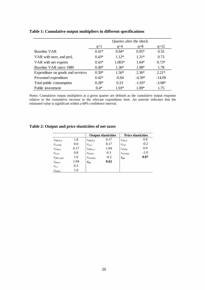
Output and price elasticities of net taxes, αt,y and αt,y, are estimated at 0.64 and 0.87,

respectively, fully in line with those in De Castro and Hernández de Cos (2008). These

are obtained as weighted averages of the elasticities of the different net-tax components,

including transfers, computed on the basis of information like statutory tax rates and

estimations of the contemporaneous responses of the different tax-bases and, in the case

of transfers, the relevant macroeconomic aggregate to GDP and price changes.

9

Furthermore, given that our main interest lies on expenditure shocks we assume

that spending decisions are prior to tax ones, which implies a zero value for βg,t. This

allows us to retrieve

gte directly and use it to estimate βt,g by OLS, which completes the

identification of the first two equations. For the remaining shocks the sequential 6 In many cases, the income tax base includes interest income as well as dividends, which in general co-vary negatively with interest rates. Nevertheless, the full set of effects of interest rate innovations on the different tax categories are very complex to analyse and, on the other hand, their contemporaneous effects are deemed to be very small. 7 The absence of contemporaneous response to real exchange rate innovations can be justified on the grounds of the popular home bias of public expenditure items, especially public consumption. 8 We took this assumption from Perotti (2004). De Castro and Hernández de Cos (2008) and Burriel et al. (2010) show that this assumption affects neither Spanish nor EMU results. 9 Further details are provided in the appendix.

7

ordering ytu , p

tu , rtu and reer

tu is imposed. The corresponding structural shocks are

estimated by instrumental variables in turn, using gte and t

te as instruments for gtu and

ttu , respectively. In any case, since we are interested in studying the effects of fiscal

policy shocks, the ordering for the remaining variables is immaterial to the results.

In what follows we present our results in terms of impulse response functions. As

usual, these are reported jointly with 68% confidence bands10

4 The effects of government spending shocks

obtained by Monte Carlo

integration methods with 1000 replications.

4.1 The baseline VAR

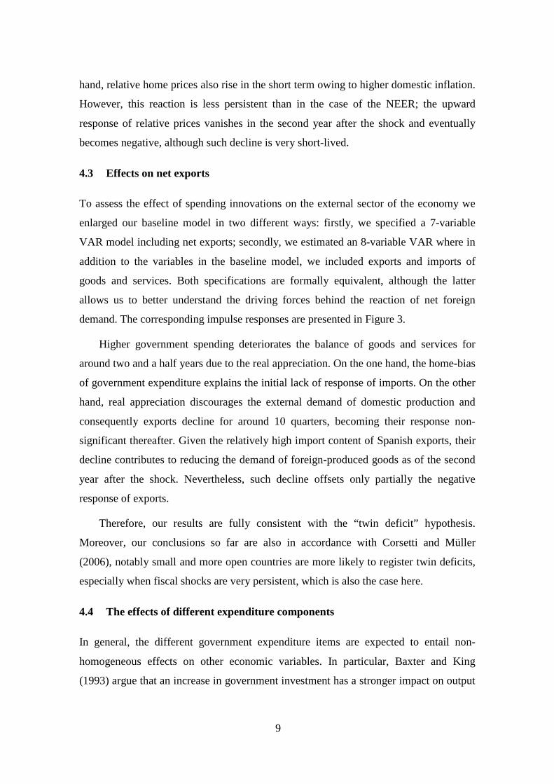
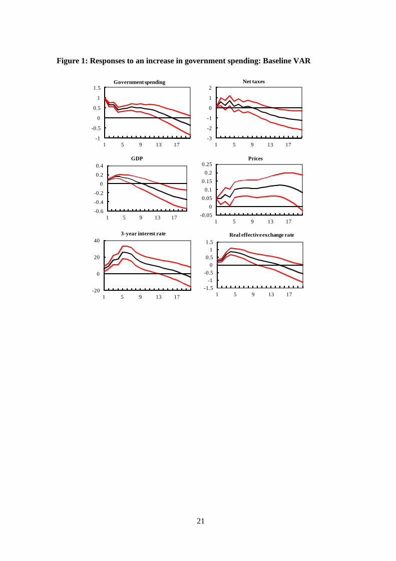
Figure 1 displays the responses of the endogenous variables to a rise in public

expenditure.11 The shock is remarkably persistent and only phases out after three years.

An increase in government expenditure entails a positive reaction of output for the first

two years following the shock, which is largely in line with previous evidence for

different countries. In general, government spending shocks are found to yield positive

output responses in the short-term as shown by Blanchard and Perotti (2002), Perotti

(2004), Fatás and Mihov (2001) or Mountford and Uhlig (2009) for the US, Heppke-

Falk et al. (2006) for Germany, De Castro (2006) and De Castro and Hernández de Cos

(2008) for Spain or Giordano et al. (2007) for Italy, although the size and persistence of

output multipliers varies significantly across studies.12 However, in the long term output

falls due to the increase in interest rates. In turn, interest rates rise owing to higher

inflation13

10 Edelberg et al. (1999), Fatás and Mihov (2001), Blanchard and Perotti (2002) or Perotti (2004) among others, also choose this bandwidth to present their results.

and higher financing needs of the government. Net taxes also go up, partly

11 Impulse responses show deviations with respect to the baseline to a one-percent shock of the relevant fiscal variable. Hence, GDP responses cannot be directly interpreted as output multipliers. 12 Caldara and Kamps (2008) show that, after controlling for differences in the specification of the reduced form model, all identification approaches used in the literature yield qualitatively and quantitatively very similar results for government spending shocks. Differences are, however, more marked in the case of tax shocks. 13 We also estimated our baseline VAR until 2009. In this case prices did not react to spending shocks, although the responses of the other variables were broadly the same. This is due to the special

8

aimed at providing funds for increased expenditure but mainly due to more buoyant

economic activity stemming from the innovation.

The real effective exchange rate appreciates in real terms in response to higher

government spending.14

However, our results in this regard oppose to Kim and Roubini (2008) for the US

for the period 1973–2002, Monacelli and Perotti (2010) for Australia, the U.S. and the

U.K. or Ravn et al. (2007) for a pool of Australia, Canada, the U.S. and the U.K., where

higher government expenditure yields real depreciations.

This pattern is consistent with not only the conventional

Mundell-Fleming model and Keynesian analysis, but also with a wide set of RBC

models under standard calibrations or with some New Keynesian formulations (see, for

instance, Corsetti et al., 2009). Accordingly, higher public spending would entail an

increase in nominal and real interest rates that would trigger capital inflows and the

subsequent appreciation. Moreover, insofar as government spending mostly

concentrates on home-produced goods, fiscal expansions should make these goods

relatively scarcer, thereby increasing their relative price with respect to imported goods

and leading to real appreciation.

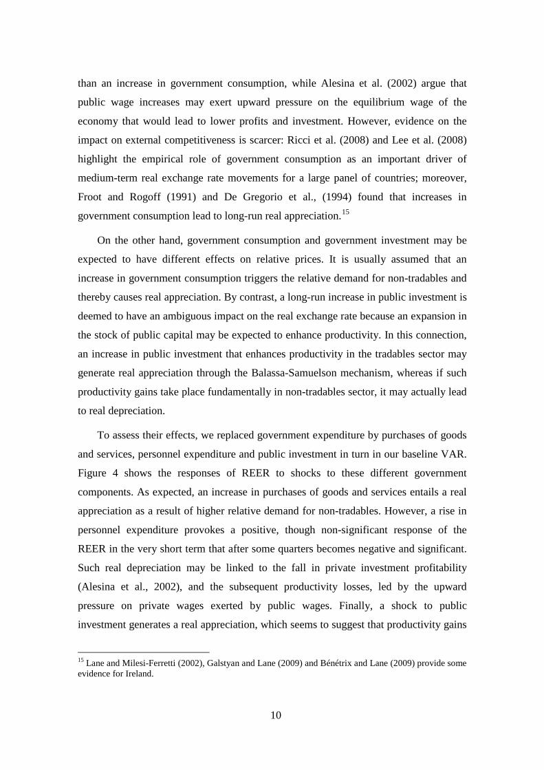
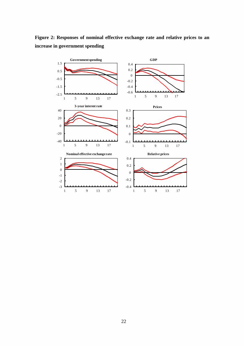
4.2 The effects on relative prices and the nominal effective exchange rate

Real appreciation driven by spending shocks can be due to nominal appreciation,

increase in relative home prices or both. In our case, since Spain is a small economy, it

seems highly unlikely that domestic spending shocks lead to significant effects on the

level of foreign prices. In order to deepen the understanding of responses of the real

effective exchange rate we substituted in our VAR the REER by the nominal effective

exchange rate (NEER) and the relative prices. Both were identified in a similar way to

REER in the baseline VAR.

Figure 2 shows that higher public spending leads to nominal appreciation as

indicated by the upward and persistent response of NEER. Such nominal appreciation is

consistent with the increase in nominal interest rates following the shock. On the other

circumstances that affected the Spanish economy that year. Specifically, a sizeable fiscal stimulus package was implemented in 2009 concomitant with the negative inflation due to the fall of bank credit. 14 Bénétrix and Lane (2009) obtain similar results for Ireland.

9

hand, relative home prices also rise in the short term owing to higher domestic inflation.

However, this reaction is less persistent than in the case of the NEER; the upward

response of relative prices vanishes in the second year after the shock and eventually

becomes negative, although such decline is very short-lived.

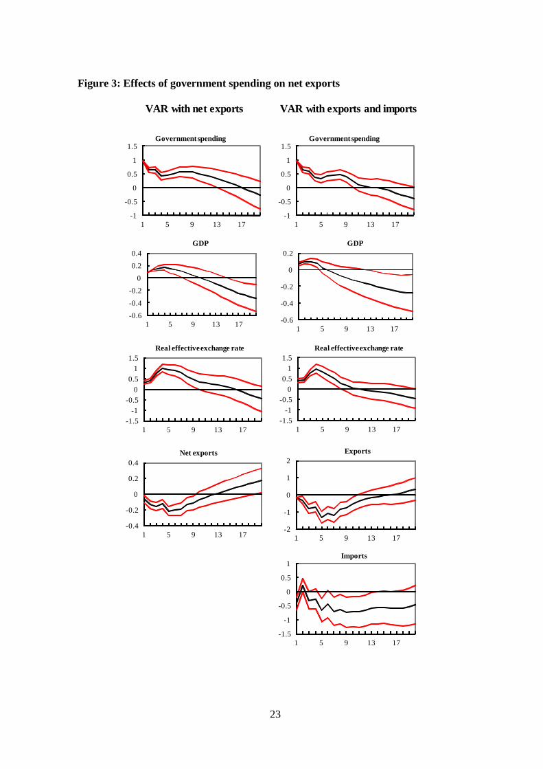
4.3 Effects on net exports

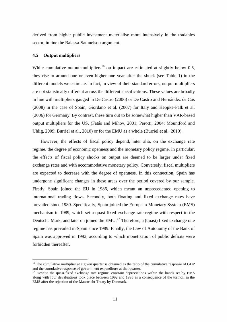
To assess the effect of spending innovations on the external sector of the economy we

enlarged our baseline model in two different ways: firstly, we specified a 7-variable

VAR model including net exports; secondly, we estimated an 8-variable VAR where in

addition to the variables in the baseline model, we included exports and imports of

goods and services. Both specifications are formally equivalent, although the latter

allows us to better understand the driving forces behind the reaction of net foreign

demand. The corresponding impulse responses are presented in Figure 3.

Higher government spending deteriorates the balance of goods and services for

around two and a half years due to the real appreciation. On the one hand, the home-bias

of government expenditure explains the initial lack of response of imports. On the other

hand, real appreciation discourages the external demand of domestic production and

consequently exports decline for around 10 quarters, becoming their response non-

significant thereafter. Given the relatively high import content of Spanish exports, their

decline contributes to reducing the demand of foreign-produced goods as of the second

year after the shock. Nevertheless, such decline offsets only partially the negative

response of exports.

Therefore, our results are fully consistent with the “twin deficit” hypothesis.

Moreover, our conclusions so far are also in accordance with Corsetti and Müller

(2006), notably small and more open countries are more likely to register twin deficits,

especially when fiscal shocks are very persistent, which is also the case here.

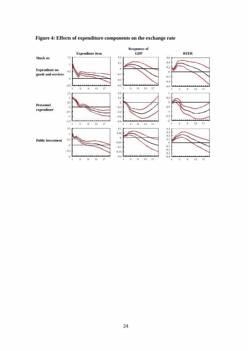
4.4 The effects of different expenditure components

In general, the different government expenditure items are expected to entail non-

homogeneous effects on other economic variables. In particular, Baxter and King

(1993) argue that an increase in government investment has a stronger impact on output

10

than an increase in government consumption, while Alesina et al. (2002) argue that

public wage increases may exert upward pressure on the equilibrium wage of the

economy that would lead to lower profits and investment. However, evidence on the

impact on external competitiveness is scarcer: Ricci et al. (2008) and Lee et al. (2008)

highlight the empirical role of government consumption as an important driver of

medium-term real exchange rate movements for a large panel of countries; moreover,

Froot and Rogoff (1991) and De Gregorio et al., (1994) found that increases in

government consumption lead to long-run real appreciation.15

On the other hand, government consumption and government investment may be

expected to have different effects on relative prices. It is usually assumed that an

increase in government consumption triggers the relative demand for non-tradables and

thereby causes real appreciation. By contrast, a long-run increase in public investment is

deemed to have an ambiguous impact on the real exchange rate because an expansion in

the stock of public capital may be expected to enhance productivity. In this connection,

an increase in public investment that enhances productivity in the tradables sector may

generate real appreciation through the Balassa-Samuelson mechanism, whereas if such

productivity gains take place fundamentally in non-tradables sector, it may actually lead

to real depreciation.

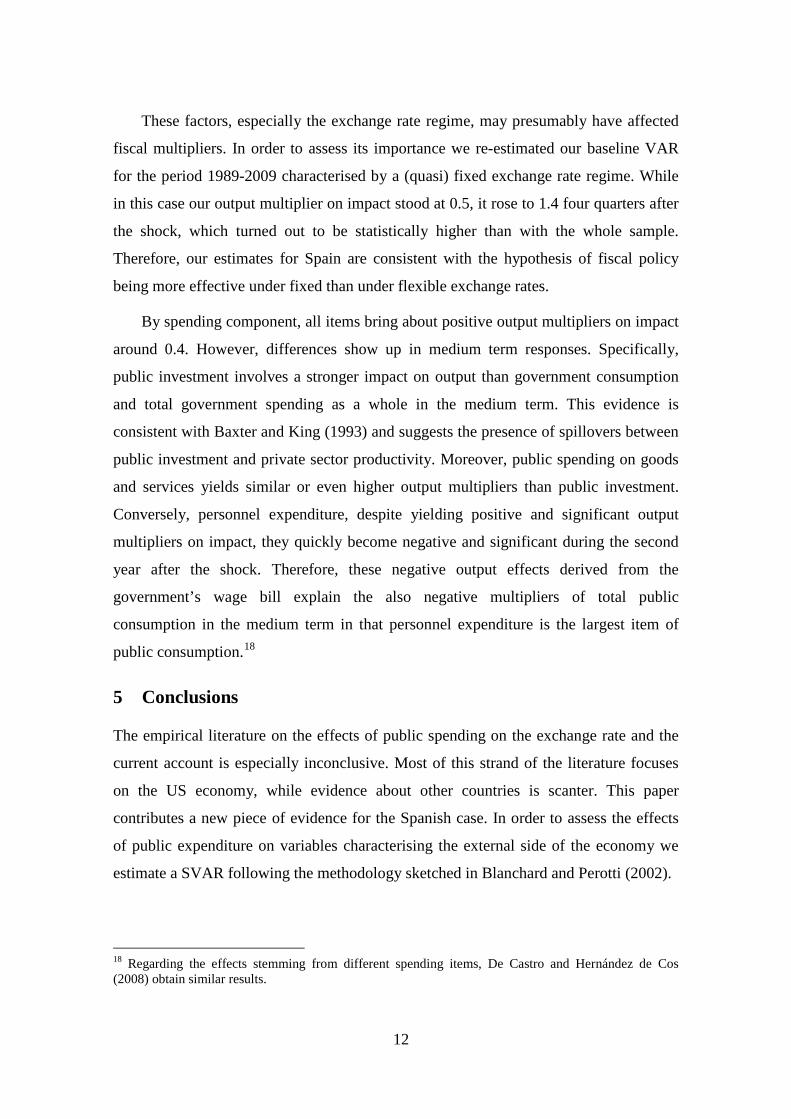
To assess their effects, we replaced government expenditure by purchases of goods

and services, personnel expenditure and public investment in turn in our baseline VAR.

Figure 4 shows the responses of REER to shocks to these different government

components. As expected, an increase in purchases of goods and services entails a real

appreciation as a result of higher relative demand for non-tradables. However, a rise in

personnel expenditure provokes a positive, though non-significant response of the

REER in the very short term that after some quarters becomes negative and significant.

Such real depreciation may be linked to the fall in private investment profitability

(Alesina et al., 2002), and the subsequent productivity losses, led by the upward

pressure on private wages exerted by public wages. Finally, a shock to public

investment generates a real appreciation, which seems to suggest that productivity gains

15 Lane and Milesi-Ferretti (2002), Galstyan and Lane (2009) and Bénétrix and Lane (2009) provide some evidence for Ireland.

11

derived from higher public investment materialise more intensively in the tradables

sector, in line the Balassa-Samuelson argument.

4.5 Output multipliers

While cumulative output multipliers16

However, the effects of fiscal policy depend, inter alia, on the exchange rate

regime, the degree of economic openness and the monetary policy regime. In particular,

the effects of fiscal policy shocks on output are deemed to be larger under fixed

exchange rates and with accommodative monetary policy. Conversely, fiscal multipliers

are expected to decrease with the degree of openness. In this connection, Spain has

undergone significant changes in these areas over the period covered by our sample.

Firstly, Spain joined the EU in 1986, which meant an unprecedented opening to

international trading flows. Secondly, both floating and fixed exchange rates have

prevailed since 1980. Specifically, Spain joined the European Monetary System (EMS)

mechanism in 1989, which set a quasi-fixed exchange rate regime with respect to the

Deutsche Mark, and later on joined the EMU.

on impact are estimated at slightly below 0.5,

they rise to around one or even higher one year after the shock (see Table 1) in the

different models we estimate. In fact, in view of their standard errors, output multipliers

are not statistically different across the different specifications. These values are broadly

in line with multipliers gauged in De Castro (2006) or De Castro and Hernández de Cos

(2008) in the case of Spain, Giordano et al. (2007) for Italy and Heppke-Falk et al.

(2006) for Germany. By contrast, these turn out to be somewhat higher than VAR-based

output multipliers for the US. (Fatás and Mihov, 2001; Perotti, 2004; Mountford and

Uhlig, 2009; Burriel et al., 2010) or for the EMU as a whole (Burriel et al., 2010).

17

16 The cumulative multiplier at a given quarter is obtained as the ratio of the cumulative response of GDP and the cumulative response of government expenditure at that quarter.

Therefore, a (quasi) fixed exchange rate

regime has prevailed in Spain since 1989. Finally, the Law of Autonomy of the Bank of

Spain was approved in 1993, according to which monetisation of public deficits were

forbidden thereafter.

17 Despite the quasi-fixed exchange rate regime, constant depreciations within the bands set by EMS along with four devaluations took place between 1992 and 1995 as a consequence of the turmoil in the EMS after the rejection of the Maastricht Treaty by Denmark.

12

These factors, especially the exchange rate regime, may presumably have affected

fiscal multipliers. In order to assess its importance we re-estimated our baseline VAR

for the period 1989-2009 characterised by a (quasi) fixed exchange rate regime. While

in this case our output multiplier on impact stood at 0.5, it rose to 1.4 four quarters after

the shock, which turned out to be statistically higher than with the whole sample.

Therefore, our estimates for Spain are consistent with the hypothesis of fiscal policy

being more effective under fixed than under flexible exchange rates.

By spending component, all items bring about positive output multipliers on impact

around 0.4. However, differences show up in medium term responses. Specifically,

public investment involves a stronger impact on output than government consumption

and total government spending as a whole in the medium term. This evidence is

consistent with Baxter and King (1993) and suggests the presence of spillovers between

public investment and private sector productivity. Moreover, public spending on goods

and services yields similar or even higher output multipliers than public investment.

Conversely, personnel expenditure, despite yielding positive and significant output

multipliers on impact, they quickly become negative and significant during the second

year after the shock. Therefore, these negative output effects derived from the

government’s wage bill explain the also negative multipliers of total public

consumption in the medium term in that personnel expenditure is the largest item of

public consumption.18

5 Conclusions

The empirical literature on the effects of public spending on the exchange rate and the

current account is especially inconclusive. Most of this strand of the literature focuses

on the US economy, while evidence about other countries is scanter. This paper

contributes a new piece of evidence for the Spanish case. In order to assess the effects

of public expenditure on variables characterising the external side of the economy we

estimate a SVAR following the methodology sketched in Blanchard and Perotti (2002).

18 Regarding the effects stemming from different spending items, De Castro and Hernández de Cos (2008) obtain similar results.

13

Our analysis shows that government spending brings about positive output

responses, jointly with real appreciation. Such real appreciation is explained by

persistent nominal appreciation and higher relative prices in the short term. In turn, the

current account deteriorates when government spending rises mainly due to the fall of

exports caused by the real appreciation. Accordingly, our results in this regard are

largely consistent not only with the conventional Mundell-Fleming model and, in

general a traditional Keynesian view, but also with a wide set of RBC or New

Keynesian models under standard calibrations. Moreover, our estimations are fully

consistent with the “twin deficits” hypothesis.

As for expenditure components, we observe that while spending on goods and

services and public investment increase output and lead to real appreciation, higher

personnel expenditure weights on economic activity and brings about real depreciation

already in the second year after the shock. Such real depreciation might be linked to

lower potential growth as a result of lower investment profitability stemming from

higher labour costs.

On the other hand, we obtain output multipliers around 0.5 on impact and slightly

above unity one year after the shock. These multipliers are in line with previous

empirical evidence regarding some individual European countries, such as Germany,

Italy or even Spain, although they seem to be on the high side when compared with

multipliers estimated for other OECD countries, including the US. Finally, we find

some evidence in favour of the hypothesis of output multipliers being higher under

fixed exchange rates in the case of Spain.

Appendix. Construction of output and price elasticities

In order to calculate the output and price elasticities we basically follow the OECD

methodology proposed in Giorno et al. (1995), which focuses on four tax categories, i.e.

personal income tax, corporate income tax, indirect taxes and social security

contributions. In addition, they consider the elasticity of transfer programmes, notably

unemployment benefits. According to this methodology, the output elasticity of the

personal income tax can be obtained as:

14

yempempwwtdirhytdirh ,,,, )1( εεεε += (A.1)

where wtdirh,ε is the elasticity of personal income tax revenues to earnings, measured by

the compensation per employee, empw,ε is the employment elasticity of the real wage

and yemp ,ε the GDP elasticity of employment. Analogously, the output elasticity of

social security contributions is:

yempempwwssyss ,,,, )1( εεεε += (A.2)

with wss,ε being the elasticity of social contributions to earnings.

The output elasticity of corporate income tax revenues stems from:

ygosgostdircytdirc ,,, εεε = (A.3)

where gostdirc,ε is the elasticity of tax revenues to the gross operating surplus and ygos,ε

the output elasticity of the gross operating surplus. In the same fashion, given that the

main tax base for indirect tax collections is private consumption, the output elasticity of

indirect taxes is obtained as:

ycctindytind ,,, εεε = (A.4)

where ctind ,ε and yc,ε are the private consumption elasticity of indirect taxes and the

output elasticity of private consumption, respectively.

Since we employ data on a national accounts basis, collection lags should not affect

the elasticities to the respective tax-bases significantly. Hence, these have been taken

from van den Noord (2000) and Bouthevillain et al. (2001). The output elasticities of

the relevant tax bases were, however, obtained from econometric estimation on a

quarterly basis. In general, the general equation used for estimating these elasticities

was:

ttiit YLnBLn ηεγ +∆+=∆ )()( (A.5)

where Bi is the relevant tax base for the ith tax category and εi is the output elasticity of

such tax base. These equations, given the likely contemporaneous correlation between

the independent variable and the error term, were estimated by instrumental variables.

15

However, if the variables Bi and Y are cointegrated, (A.5) contains a specification error.

In this case, the following ECM specification would be preferable:

tk

j

ijtj

k

jjtj

titit

it

BLnYLn

YLnYLnBLnBLn

ηνϕ

εφλµγ

+∆+∆+

∆+−−+=∆

∑∑=

−=

−

−−

11

11

)()(

)())()(()( (A.6)

where λ measures the long-term contemporaneous elasticity we are interested in.

Information on the output elasticity of net transfers is more limited than in the

former cases. Although unemployment benefits respond to the underlying economic

conditions, many expenditure programmes do not have built-in conditions that make

them respond contemporaneously to employment or output. Therefore, recalling

Perotti’s argument, an output elasticity of net transfers of -0.2 has been assumed.

As for price elasticities, following van der Noord (2000) those of direct taxes paid

by households, corporate income taxes and social contributions were obtained as

1,, −= wtdirhptdirh εε , 1,, −= gostdircptdirc εε and 1,, −= wsspss εε , respectively.

Indirect taxes are typically proportional. Hence, following Perotti (2004), a zero price

elasticity was assumed. Finally, although transfer programmes are indexed to the CPI,

indexation occurs with a considerable lag. Thus, the price elasticity of transfers was set

to -1.

Accordingly, contemporaneous output elasticities of net taxes can be calculated as:

TTi

yBi

BTyt iii ,,, εεα ∑= (A.7)

with ∑= iTT being the level of net taxes19ii BT ,ε, the elasticity of the ith category of net

taxes to its own tax base and yBi ,ε the GDP elasticity of the tax base of the ith category

of net taxes. Price elasticities are obtained in a similar fashion. Table 2 shows the

resulting output and price elasticities.

19 The Ti’s are positive in the case of taxes and negative in the case of transfers.

16

References

Afonso, A. and R. M. Sousa (2009a). The macroeconomic effects of fiscal policy. ECB

Working Paper Series No. 991, January.

Afonso, A. and R. M. Sousa (2009b). The macroeconomic effects of fiscal policy in

Portugal: a Bayesian SVAR analysis. School of Economics and Management,

Working Papers Nº 09/2009/DE/UECE.

Alesina, A., S. Ardagna, R. Perotti, and F. Schiantarelli (2002). Fiscal Policy, Profits

and Investment. American Economic Review 92, pp. 571-589.

Baxter, M. and R. King (1993). Fiscal policy in general equilibrium. American

Economic Review, 83, pp. 315-334.

Beetsma, R., M. Giuliodori and F. Klaassen (2008). The Effects of Public Spending

Shocks on Trade Balances and Budget Deficits in the European Union. Journal of

the European Economic Association, 6(2-3), pp. 414-423.

Bénassy-Quéré, A. and J. Cimadomo (2006). Changing patterns of domestic and cross-

border fiscal policy multipliers in Europe and the US. CEPII WP #2006-24.

Bénétrix, A. S. and Lane, P.R. (2009). The impact of fiscal shocks on the Irish

economy. The Economic and Social Review, 40(4), pp. 407-434.

Blanchard, O. J. and R. Perotti (2002). An Empirical Characterization of the Dynamic

Effects of Changes in Government Spending and Taxes on Output. Quarterly

Journal of Economics, 117, pp. 1329-1368.

Bouthevillain, C., Cour-Thimann, P., van den Dool, G., Hernández de Cos, P.,

Langenus, G., Mohr, M., Momigliano, S., Tujula, M., 2001. Cyclically adjusted

budget balances: An alternative approach. ECB Working Paper Series No. 77.

Burriel, P., F. de Castro, D. Garrote, E. Gordo, J. Paredes and J. J. Pérez (2010). Fiscal

policy shocks in the euro area and the US: an empirical assessment. Fiscal Studies

31 (2), pp. 251-285.

17

Caldara, D. and C. Kamps (2008). What are the effects of fiscal policy shocks? A VAR-

based comparative analysis. ECB Working Paper Series No. 877, March.

Corsetti, G., A. Meier and G. Müller (2009). Fiscal Stimulus with Spending Reversals,

IMF Working Paper WP/097106.

de Castro, F. (2006). The macroeconomic effects of fiscal policy in Spain. Applied

Economics, 38, pp. 913-924.

de Castro, F and P. Hernández de Cos (2008). The economic effects of fiscal policy: the

case of Spain. Journal of Macroeconomics, 30, pp. 1005-1028.

De Gregorio, J., A. Giovannini and H. Wolf (1994). International Evidence on

Tradables and Nontradables Inflation. European Economic Review, 38, pp. 1225-

1244.

Edelberg, W., M. Eichenbaum, and J.D.M. Fisher (1999). Understanding the Effects of

a Shock to Government Purchases. Review of Economic Dynamics, 2, pp. 166-

206.

Enders, Z., G. Müller and A. Scholl (2011). How do Fiscal and Technology Shocks

affect Real Exchange Rates? New Evidence for the United States. Journal of

International Economics 83(1), pp. 53-69.

Estrada, A., J.L. Fernández, E. Moral,and A.V. Regil (2004). A quarterly

macroeconometric model of the Spanish economy. Banco de España Working

Paper No. 0413.

Fatás, A. and I. Mihov (2001). The effects of fiscal policy on consumption and

employment: theory and evidence. CEPR Discussion Paper Series No. 2760.

Frenkel, J.A. and A. Razin (1996). Fiscal Policies and Growth in the World Economy,

Third Edition. MIT Press, Cambridge, MA.

K. Froot, and K. Rogoff (1991). The EMS, the EMU, and the Transition to a Common

Currency. NBER Macroeconomics Annual, Vol. 6, pp. 269-317.

Galstyan, V. and P.R. Lane (2009). Fiscal policy and international competitiveness:

evidence for Ireland. The Economic and Social Review, 40(3), pp. 299–315.

18

Giordano, R., S. Momigliano, S. Neri and R. Perotti (2007). The effects of fiscal policy

in Italy: Evidence from a VAR model. European Journal of Political Economy,

23, pp. 707–733.

Giorno, C., P. Richardson, D. Roseveare and P. van den Noord (1995). Potential output,

output gaps and structural budget balances. OECD Economic Studies 24.

Heppke-Falk, K.H., J. Tenhofen and G.B. Wolff (2006). The macroeconomic effects of

exogenous fiscal policy shocks in Germany: a disaggregated SVAR analysis.

Deutsche Bundesbank. Discussion Paper Series 1: Economic Studies No 41/2006.

Kim, S., and N. Roubini (2008). Twin deficit or twin divergence? Fiscal policy, current

account, and real exchange rate in the U.S. Journal of International Economics,

74(2), pp. 362–383.

Lane, P.R. and G. M. Milesi-Ferretti (2002). Long-Run determinants of the Irish real

exchange rate. Applied Economics, 34(5), pp. 549-55.

Lee, J., G. M. Milesi-Ferretti, J. Ostry, A. Prati and L. Ricci (2008). Exchange Rate

Assessments: CGER Methodologies. IMF Occasional Paper No. 261.

Marcellino, M. (2006). Some stylized facts on non-systematic fiscal policy in the euro

area. Journal of Macroeconomics, 28, pp. 461-479.

Monacelli, T. and R. Perotti (2010). Fiscal Policy, the Real Exchange Rate and Traded

Goods. The Economic Journal, 120, pp 437–461.

Mountford, A. and H. Uhlig (2009). What are the effects of fiscal policy shocks?.

Journal of Applied Econometrics, 24, pp. 960–992.

Obstfeld, M. and K. Rogoff (1995). Exchange rate dynamics redux. Journal of Political

Economy, 103, pp. 624–660.

Perotti, R. (2004). Estimating the effects of fiscal policy in OECD countries.

Proceedings, Federal Reserve Bank of San Francisco.

Ravn, M.O., S. Schmitt-Grohé and M. Uribe (2007). Explaining the effects of

government spending on consumption and the real exchange rate. NBER Working

Paper Series No. 13328.

19

Ricci, L., G. M. Milesi-Ferretti and J. Lee (2008). Real Exchange Rates and

Fundamentals: A Cross-Country Perspective. IMF Working Paper No. 08/13.

van den Noord, P. (2000). The size and role of automatic fiscal stabilizers in the 1990s

and beyond. OECD Working Paper No. 230.

20

Table 1: Cumulative output multipliers in different specifications

Notes: Cumulative output multipliers at a given quarter are defined as the cumulative output response relative to the cumulative increase in the relevant expenditure item. An asterisk indicates that the estimated value is significant within a 68% confidence interval.

Table 2: Output and price elasticities of net taxes

Output elasticities Price elasticities εtdirh,w 1.8 εtdirh,y 0.17 εtdir,p 0.8 εw,emp 0.0 εss,y 0.17 εss,p -0.2 εemp,y 0.17 εtdirc,y 1.04 εtind,p 0.0 εss,w 0.8 εtind,y 0.3 εtransf,p -1.0 εtdirc,gos 1.0 εtransf,y -0.2 εt,p 0.87 εgos,y 1.04 εt,y 0.62 εc,y 0.3 εtind,c 1.0

q=1 q=4 q=8 q=12Baseline VAR 0.41* 0.94* 0.95* 0.55VAR with neert and prelt 0.43* 1.12* 1.21* 0.73VAR with net exports 0.43* 1.003* 1.04* 0.73*Baseline VAR since 1989 0.49* 1.36* 1.98* 1.78Expenditure on goods and services 0.39* 1.56* 2.36* 2.21*Personnel expenditure 0.42* -0.64 -4.59* -14.09Total public consumption 0.28* 0.23 -1.03* -3.08*Public investment 0.4* 1.03* 1.89* 1.75

Quartes after the shock

21

Figure 1: Responses to an increase in government spending: Baseline VAR

-1

-0.5

0

0.5

1

1.5

1 5 9 13 17

Government spending

-3

-2

-1

0

1

2

1 5 9 13 17

Net taxes

-20

0

20

40

1 5 9 13 17

3-year interest rate

-1.5-1

-0.50

0.51

1.5

1 5 9 13 17

Real effective exchange rate

-0.050

0.050.1

0.150.2

0.25

1 5 9 13 17

Prices

-0.6

-0.4

-0.2

0

0.2

0.4

1 5 9 13 17

GDP

22

Figure 2: Responses of nominal effective exchange rate and relative prices to an

increase in government spending

-2.5

-1.5

-0.5

0.5

1.5

1 5 9 13 17

Government spending

-0.1

0

0.1

0.2

0.3

1 5 9 13 17

Prices

-0.6

-0.4

-0.2

0

0.2

0.4

1 5 9 13 17

GDP

-40

-20

0

20

40

1 5 9 13 17

3-year interest rate

-3

-2

-1

0

1

2

1 5 9 13 17

Nominal effective exchange rate

-0.4

-0.2

0

0.2

0.4

1 5 9 13 17

Relative prices

23

Figure 3: Effects of government spending on net exports

VAR with exports and importsVAR with net exports

-1.5-1

-0.50

0.51

1.5

1 5 9 13 17

Real effective exchange rate

-1

-0.5

0

0.5

1

1.5

1 5 9 13 17

Government spending

-0.6

-0.4

-0.2

0

0.2

1 5 9 13 17

GDP

-2

-1

0

1

2

1 5 9 13 17

Exports

-1.5

-1

-0.5

0

0.5

1

1 5 9 13 17

Imports

-1

-0.5

0

0.5

1

1.5

1 5 9 13 17

Government spending

-0.6

-0.4

-0.2

0

0.2

0.4

1 5 9 13 17

GDP

-1.5-1

-0.50

0.51

1.5

1 5 9 13 17

Real effective exchange rate

-0.4

-0.2

0

0.2

0.4

1 5 9 13 17

Net exports

24

Figure 4: Effects of expenditure components on the exchange rate

Shock to:

Expenditure ongoods and services

Personnel expenditure

Public investment

Expenditure item GDP REERResponses of

-0.5

0

0.5

1

1.5

1 5 9 13 17-0.3

-0.2

-0.1

0

0.1

0.2

1 5 9 13 17-0.6

-0.4

-0.2

0

0.2

0.4

0.6

1 5 9 13 17

-1.5

-1

-0.5

0

0.5

1

1.5

1 5 9 13 17-0.8

-0.6

-0.4

-0.2

0

0.2

0.4

1 5 9 13 17-2

-1.5

-1

-0.5

0

0.5

1

1 5 9 13 17

-1

-0.5

0

0.5

1

1.5

1 5 9 13 17-0.2

-0.15

-0.1

-0.05

0

0.05

0.1

1 5 9 13 17-0.4-0.3-0.2-0.1

00.10.20.30.4

1 5 9 13 17