Embed Size (px)
Citation preview

Forschungsinstitut zur Zukunft der ArbeitInstitute for the Study of Labor
DI
SC
US
SI
ON
P
AP
ER
S
ER
IE
S
The Economic Contribution of Unauthorized Workers: An Industry Analysis
IZA DP No. 10366
November 2016
Ryan EdwardsFrancesc Ortega

The Economic Contribution of
Unauthorized Workers: An Industry Analysis
Ryan Edwards Queens College, CUNY
Francesc Ortega Queens College, CUNY
and IZA
Discussion Paper No. 10366 November 2016
IZA
P.O. Box 7240 53072 Bonn
Germany
Phone: +49-228-3894-0 Fax: +49-228-3894-180
E-mail: [email protected]
Any opinions expressed here are those of the author(s) and not those of IZA. Research published in this series may include views on policy, but the institute itself takes no institutional policy positions. The IZA research network is committed to the IZA Guiding Principles of Research Integrity. The Institute for the Study of Labor (IZA) in Bonn is a local and virtual international research center and a place of communication between science, politics and business. IZA is an independent nonprofit organization supported by Deutsche Post Foundation. The center is associated with the University of Bonn and offers a stimulating research environment through its international network, workshops and conferences, data service, project support, research visits and doctoral program. IZA engages in (i) original and internationally competitive research in all fields of labor economics, (ii) development of policy concepts, and (iii) dissemination of research results and concepts to the interested public. IZA Discussion Papers often represent preliminary work and are circulated to encourage discussion. Citation of such a paper should account for its provisional character. A revised version may be available directly from the author.

IZA Discussion Paper No. 10366 November 2016
ABSTRACT
The Economic Contribution of Unauthorized Workers: An Industry Analysis*
This paper provides a quantitative assessment of the economic contribution of unauthorized workers to the U.S. economy, and the potential gains from legalization. We employ a theoretical framework that allows for multiple industries and a heterogeneous workforce in terms of skills and productivity. Capital and labor are the inputs in production and the different types of labor are combined in a multi-nest CES framework that builds on Borjas (2003) and Ottaviano and Peri (2012). The model is calibrated using data on the characteristics of the workforce, including an indicator for imputed unauthorized status (Center for Migration Studies, 2014), and industry output from the Bureau of Economic Analysis. Our results show that the economic contribution of unauthorized workers to the U.S. economy is substantial, at approximately 3% of private-sector GDP annually, which amounts to close to $5 trillion over a 10-year period. These effects on production are smaller than the share of unauthorized workers in employment, which is close to 5%. The reason is that unauthorized workers are less skilled and appear to be less productive, on average, than natives and legal immigrants with the same observable skills. We also find that legalization of unauthorized workers would increase their contribution to 3.6% of private-sector GDP. The source of these gains stems from the productivity increase arising from the expanded labor market opportunities for these workers which, in turn, would lead to an increase in capital investment by employers. JEL Classification: D7, F22, H52, H75, J61, I22, I24 Keywords: immigration, unauthorized, industry, contribution Corresponding author: Francesc Ortega Department of Economics Queens College, CUNY 300A Powdermaker Hall 65-30 Kissena Blvd. Queens, New York 11367 USA E-mail: [email protected]
* Edwards’s work is directly supported by funds from the Center for American Progress (CAP). Ortega is grateful to CAP for funding this project. We thank Agustin Indaco, Sarah Bohn, Deborah Cobb-Clark, Gretchen Donehower, Delia Furtado, Chinhui Juhn, Giev Kashkooli, Ed Kissam, Phil Martin, Pia Orrenius, Manuel Pastor, Jennifer Van Hook, Bob Warren, and Robert Warren for helpful comments. All errors are our own.

1 Introduction
There is wide consensus that the problem of the large unauthorized population in the United
States needs to be addressed soon.1 A crucial input into the debate is an assessment of
the economic contribution of unauthorized workers, and the potential gains from legalizing
these workers. The main goal of our project is to offer such a quantitative assessment
using a state-of-the-art theoretical framework that accounts for the large heterogeneity in
the characteristics of the unauthorized workers that we observe in the data, and for the
complementarities in production between these workers and the rest of the workforce.
More specifically, we adopt the multi-nest CES theoretical framework proposed by Borjas
(2003) and Ottaviano and Peri (2012), and adapt it to analyze the contributions to output of
unauthorized workers at the industry level. We calibrate the model using data from a special
extract of the American Community Survey (years 2011-2013) provided by the Center for
Migration Studies (2014), which contains a variable that assigns documentation status to all
foreign-born workers in the sample along with detailed information on employment, skills
and wages, and the Bureau of Economic Analysis’ National Accounts.2 We then conduct
simulations at the industry level to quantify the economic contribution of unauthorized
workers to the level of production in the industry. We do so by comparing industry output as
currently observed in the data to output in a counterfactual without unauthorized workers.
Similarly, we also conduct simulations of the economic effects of providing legal status to
these workers. We distinguish between short and long-run effects, where the latter scenario
takes into account the adjustment to the capital stock following changes in the workforce.
A large body of literature has analyzed the labor market effects of immigration. Most
studies in this literature estimate reduced-form models or econometric specifications derived
from highly simplified models. In a very influential study, Borjas (2003) presented a multi-
nest CES production model that emphasized the role of complementarities in production
and allowed for a clear discussion of within and between skill group effects. Manacorda et
al. (2012) and Ottaviano and Peri (2012) further extended the theoretical setup to allow
for imperfect substitution in production between natives and immigrants with the same
education and potential experience. We adopt their theoretical framework, extend it to
consider documentation status, adding a new level to the multi-nest CES framework. As
we argue later, for our purpose of estimating the contribution of unauthorized workers to
1Several European countries also have, or have had in the recent past, a large unauthorized populationwithin their borders. For a recent review, see Orrenius and Zavodny (2016).
2We describe these data and the documentation status imputation in Section 2.
1

production, the calibration of the productivity terms for each type of labor is much more
important quantitatively than the parametrization of the elasticities of substitution.
Our work is also related to the studies that estimate the effects of legalization and
naturalization. The vast majority of these studies focus on the effects on the earnings of
immigrants (Chiswick (1978), Bratsberg et al. (2002), Kossoudji and Cobb-Clark (2002),
Lofstrom et al. (2013), Lynch and Oakford (2013), and Pastor and Scoggins (2012), among
others). Instead our focus is on overall income and output at the industry level. Because of
our interest on the aggregate income effects of unauthorized immigration, our study is more
closely related to the work of Lynch and Oakford (2013). These authors study the effects
of legalization and citizenship on U.S. GDP, in addition to several other outcomes, such
as employment, tax revenues and earnings of the immigrants themselves. They conclude
that granting legal status and citizenship to unauthorized immigrants will increase their
income by 25 percent, with roughly similar contribution from legalization and naturaliza-
tion. Projecting over a 10-year period their estimates imply a cumulative increase in GDP
of approximately $1.4 trillion.3
Relative to the existing literature, our analysis of the economic contribution of unau-
thorized workers is novel in several dimensions. First, we focus on the effects on the level
of production at the industry level. Second, our analysis is based on a fully specified eco-
nomic model that we calibrate using a combination aggregate and individual level data.
This model accounts for the degree of complementarities in production between different
types of workers, and allows us to assess the role played by these somewhat controversial
parameters on the results. In addition we show that the model can be calibrated to in-
corporate the large heterogeneity among the unauthorized workforce in terms of skills and
productivity. Finally, an important benefit of our structural approach is that we can sim-
ulate policy-relevant counterfactual scenarios, such as the removal of unauthorized workers
or their legalization. To the best of our knowledge, our study is the first one providing
estimates of the contribution of unauthorized workers along with the potential gains from
providing legal access to these workers.
Our descriptive analysis of the data reveals some interesting patterns that play an impor-
tant role in our simulation results. First, we document the large variation across industries
in the share of unauthorized workers. Specifically, in the period 2011-2013 the share of
unauthorized workers in employment is highest in Agriculture (18%), Construction (13%)
3Their estimates build on the study of the effects of 1986 IRCA conducted by the Department of Labor(1996), which concluded that legalization led to a 15 percent increase in the earnings of unauthorizedimmigrants between 1986 and 1992.
2

and Leisure and hospitality (10%), well above the national average of 4.9%. Our data
also reveal important differences in average wages by industry, nativity and documentation
status. In most industries legal immigrants and natives have similar earnings, while the
earnings of unauthorized workers are substantially lower. Naturally, these wage differences
reflect, to a large extent differences in skills. In our data unauthorized immigrants have an
average of 3 years of schooling less than the average U.S.-born and legal immigrant worker.
Nonetheless unauthorized workers are not a homogeneous group, displaying large differences
in educational attainment by industry of employment.
We can now turn to our main results. The simulation of the counterfactual where
unauthorized workers are removed from each industry at a time reveals that these workers
are responsible for about 3% of private-sector GDP, which amounts to approximately $5
trillion over a 10-year period. At first the removal of unauthorized workers would reduce
aggregate production by about 1.7%, but the loss would be magnified as employers downsize
the stock of capital in order to match the reduced workforce. These aggregate estimates hide
large differences across industries, largely reflecting the shares of unauthorized workers in
industry employment. Once capital has adjusted, value-added in Agriculture, Construction
and Leisure and hospitality would fall by 8-9%. However, the largest losses in dollars
would take place in Manufacturing, Wholesale and retail trade, Finance and Leisure and
hospitality. Likewise we also find large differences across states that largely reflect the
employment shares of unauthorized workers in each state, along with the state’s industry
specialization.
We also note that even though unauthorized workers are about 5% of employment, their
contribution to private-sector GDP is around 3%. This is due to differences in productiv-
ity between these workers and the rest of the workforce. While part of the productivity
differential is due to the lower measured skills, our calibration procedure also reveals large
residual differences in productivity, after controlling for measured educational attainment
and potential experience.
In order to gauge the role played by the challenges imposed by the lack of legal status
on the productivity of unauthorized workers, we simulate a scenario where unauthorized
workers are assumed to have the same productivity as legal immigrant workers with the
same levels of education and potential experience.4
4To the extent that acquiring legal status might induce undocumented immigrant workers to acquire morehuman capital or switch industry of employment, our estimates should be interpreted as a lower-bound onthe economic effects of legalization. Indeed Rivera-Batiz (1999) provides some evidence of skill upgradingfollowing legalization.
3

Because documented foreign-born workers are about 25% more productive than undoc-
umented ones with the same levels of education and experience, legalization would have a
large effect on the earnings of undocumented workers. The consequences in terms of in-
dustry production would be much more muted. After adjustments in the stock of capital,
industry GDP would increase by 1-2% in Agriculture, Construction and Leisure and hospi-
tality. For the economy as a whole, our results suggest an increase in private-sector GDP
of about 0.6%.
The structure of the paper is as follows. In Section 2 we describe our data. Section 3
presents descriptive statistics. Section 4 describes our model. Section 5 describes our cali-
bration of the parameters. Section 6 defines our counterfactual scenarios, while Section 7
reports our main results. Section 8 discusses some caveats and Section 9 gathers our con-
clusions.
2 Data
2.1 Sources
Most of our analysis draws from special extracts of the American Community Survey (ACS)
of the U.S. Census Bureau for the years 2011, 2012, and 2013 provided by the Center for
Migration Studies (2014). Our pooled sample across these three years contains 9,357,842
individuals in total, 4,154,227 of whom report employment.
The key variable in our analysis is an individual-level measure of imputed undocumented
status, a binary indicator for every record in the ACS. Although the ACS does not ask about
legal status per se, it does ask about citizenship, country of birth, and year of immigration,
in addition to a wide array of demographic and socioeconomic characteristics including
employment status. The specific methodology used to impute authorized status is described
in detail in Warren (2014), and we summarize it here.
The procedure is essentially a two-step process. In the first step, the overall size of
the undocumented population is obtained starting from Census estimates of total foreign-
born residents and subtracting accumulated counts of legalized foreign born residents drawn
from official statistics kept by the U.S. Department of Homeland Security. The second step
imputes documentation status at the individual level. First developed by Passel and Clark
(1998) for the Urban Institute, the method has continued to evolve within government and
policy circles. Recent contributions include those by Baker and Rytina (2013), Warren and
Warren (2013), and Passel and Cohn (2014, 2015), in addition to Warren (2014). Each of
4

these efforts utilizes survey information to identify foreign-born respondents in the CPS or
ACS who are likely to be unauthorized based on their characteristics. Chief among these
characteristics that indicate likely documented status are year of arrival, because of the
amnesty granted under the Immigration Reform and Control Act of 1986 (IRCA). Other
key variables used in the imputation procedure are country of origin, occupation, industry,
and receipt of government benefits. Workers with certain occupations that require licensing,
such as legal professions, police and fire, and some medical professions, are assumed to be
authorized, as well as individuals in government or in the military.5
Existing estimates of the characteristics of the imputed unauthorized population ob-
tained from the Census, the ACS and the CPS tend to be largely consistent with each other,
indicating “face validity” (Warren, 2014). In a recent study, Pastor and Scoggins (2016)
provide a comparison between several of the existing approaches to estimate the unautho-
rized population or subsets of it. Reassuringly, the results are fairly consistent across these
studies. Likewise, the imputation carried out by Borjas (2016) also provides additional
confirmation. The broader validity of these types of estimates is less clear. Assessments
remain constrained by the nature of the problem; without large representative surveys that
ask legal status, it is unclear how to produce comparable but alternative measures of the
truth.6
In addition to these data, our calibration also makes use of the GDP estimates produced
by the Bureau of Economic Analysis (BEA). Our industry definitions consist of conventional
“one-digit” industries identified via the North American Industry Classification System
(NAICS) as used by Passel and Cohn (2015) and others. Specifically, we focus on the
industries 1-12 below, which are often referred to as private-sector GDP:
1. Agriculture, forestry, fishing, hunting 8. Financial activities2. Mining 9. Professional and business services3. Construction 10. Educational and health services4. Manufacturing 11. Leisure and hospitality5. Wholesale and retail trade 12. Other services6. Transportation and utilities 13. Government7. Information
Combined these thirteen industries produce all of national GDP. As we discussed earlier,
5Anecdotal evidence shows that there are some unauthorized workers in these industries, particularly inthe military. Nevertheless the size of this group is negligible.
6The Survey of Income and Program Participation (SIPP), also a Census product, directly asks respon-dents about legal status but is roughly one sixth the size of the ACS. Using the SIPP as their baseline oftruth, Van Hook et al. (2015) show that imputed legal status within Census products such as ACS canproduce significant bias in estimates of outcomes that are directly linked to legal status, such as healthinsurance coverage. For our purposes this concern is probably less relevant.
5
our imputations of authorized status assume that there are no undocumented workers in
public administration or the military, so we omit this industry from consideration.
2.2 Sample definitions
Because the calibration of our model will draw from Ottaviano and Peri (2012), we build
skill cells closely following their definitions. We classify workers within each industry (and
state) as belonging to one out of 96 possible categories on the basis of their education, po-
tential experience, nativity and documentation status. We consider 4 educational groups:
individuals with either 0–11 years, 12 years, 13–15 years, or 16 years and more of school-
ing. Potential experience measures years since the last year of schooling, and we build 8
categories: 1–5, 6–10, 11–15, 16–20, 21–25, 26–30, 31–35, or 36–40 years.
To build our samples we pool observations across the 2011, 2012, and 2013 waves of the
ACS data in the CMS extracts, taking simple averages of quantities within each cell and
weighted averages of dollar amounts converted to 2013 dollars using the consumer price
index. We build two slightly different samples.
Following Ottaviano and Peri, our wage sample drops individuals with potential ex-
perience less than 1 or greater than 40, eliminating workers at the extremes of the age
distribution. We further eliminate individuals living in group quarters, those younger than
18, those who reported not working last year, those who did not report valid salary in-
come, and the self-employed. We use the wage sample to calibrate the worker productivity
parameters in the model.
Our employment sample is more inclusive and includes all valid observations of em-
ployed workers within the ACS. In this sample definition, we treat experience groupings as
bottom and top-coded, including those with less than 1 year of potential experience into
the first experience group and those with more than 40 years into the top experience group.
The worker counts (and hours worked) obtained from this sample will be the basis for the
construction of our labor aggregates in each industry (and state).
3 Descriptive statistics
There is great heterogeneity in the distribution of unauthorized workers across industries
and states in the United States. While the share of undocumented workers in employment is
4.9 percent for the U.S. as a whole, this figure is much higher in some states. In California,
the employment share of undocumented workers is 10.2 percent, and it ranges between 6.2
6

and 8.7 percent in Texas, Nevada, New Jersey and New York.7
Likewise, the distribution of unauthorized workers across industries varies widely, as il-
lustrated by Table 1. Of the roughly 7.1 million undocumented foreign-born workers in the
U.S. in 2011–2013, the largest concentrations are found in the Leisure and Hospitality sector
(1.3 million), Construction (1.1 million), Professional and Business services (1.0 million),
and Manufacturing (0.9 million). However, the industries with the highest undocumented
shares are Agriculture (18 percent),8 Construction (13 percent), and Leisure and Hospital-
ity (10 percent), as can be seen in column 4.9 In other industries, the undocumented are
smaller shares of total employment, but they are never absent altogether except from Gov-
ernment (due to the design of the imputation procedure). Even in industries with relatively
high education requirements, such as Finance and Information, undocumented immigrants
account for about 2 percent of the workforce.
Although their numbers and shares of unauthorized immigrants have been declining in
recent years (Passel and Cohn, 2014), roughly half of unauthorized immigrants are Mexican.
Table 2 reports a breakdown of unauthorized workers by national origin (Mexico, Central
and South America, Asia and Others) and industry. According to our data 3.8 million
unauthorized workers (55% of the total) are Mexican, 1.8 million (26%) originate from
Central and South America, and 0.9 million from Asia (13%). The industries employing the
highest numbers of unauthorized Mexican workers are Leisure and Hospitality (0.78 million)
and Construction (0.74 million). These two industries also employ the highest numbers of
Central and South American unauthorized workers. In contrast, the industries that employ
the highest numbers of Asian unauthorized workers are Professional and business services
(0.17 million), Leisure and hospitality (0.14 million) and Wholesale and retail trade (0.14
million).
Our data also reveal large difference in weekly earnings across industries, nativity and
documentation status. As displayed in Table 3, on average across all industries, the weekly
wages for U.S.-born workers are $1,039. Legal immigrants earn, on average, slightly more
($1,050). In comparison the earnings of unauthorized workers are about 40 percent lower
($581 per week). This ordinal ranking of wages is observed in several industries, although
natives earn on average more than legal immigrants in some industries. In Agriculture, the
7In absolute numbers, the five states with the most undocumented workers are California, Texas, NewYork, Florida, and Illinois (Table 12).
8The foreign-born share in Agriculture may be substantially higher than the ACS implies because of thehigh prevalence of seasonal workers.
9Note also that these shares are practically unchanged if we compute them on the basis of hours worked(as in column 6), rather than employment.
7

weekly earnings of natives, documented foreign-born and undocumented foreign-born are
$734, $491 and $378. Likewise in Construction natives earn $962, compared to $803 and
$510 for documented and undocumented immigrants, respectively. In contrast, in Educa-
tional and health services, the highest earnings correspond to legal immigrants ($1,115),
followed by natives ($962) and by undocumented immigrants ($641).
It is also interesting to scrutinize further the large variation in the average weekly
wages earned by unauthorized workers across industries, shown in the rightmost column
of Table 3. Across industries we observe large differences, ranging from the roughly $400
paid in Agriculture and Leisure and hospitality to these workers, to the approximately
$1,300 paid in the Information sector.
To some extent these differences in average wages are due to the higher concentra-
tion of undocumented workers in low-wage industries, such as Leisure and hospitality or
Agriculture. As one would expect, the differences in average wages that remain when we
condition on industry of employed are partly due to differences in educational attainment
and in (potential) work experience. As documented in Table 4, native and foreign-born
workers with legal status have, respectively, 13.9 and 13.3 years of education, which is al-
most 3 years more than the average undocumented worker (10.6 years). Similarly, native
and legal foreign-born workers have 3.4 and 5.8 years of potential experience more than
undocumented immigrants (Table 5). Nonetheless, as we discuss later (in the calibration),
residual productivity differences also play an important role in accounting for wage differ-
ences by nativity and documentation status, after accounting for industry of employment,
and measured education and potential experience.
4 Theoretical framework
The economy consists of j = 1, ..., J industries. Output in industry j is produced by means
of a constant-returns Cobb-Douglas production function:
Yj = AjKαjj L
1−αjj , (1)
where αj ∈ (0, 1) is the capital share in industry j.
4.1 Labor Aggregate
Let us now describe in detail the labor aggregate, L, in the previous equation.10 We allow
workers to differ in education (e = 1, ..., E), potential years of work experience (x = 1, ..., X),
10To simplify our notation we now omit the industry j subindex.
8

nativity (U.S.-born or foreign-born) and, if foreign-born, also by documentation status. In
total the number of labor types is given by 3× E ×X.
We aggregate all these types of workers by means of a multi-nested constant-elasticity
of substitution (CES) aggregator.11 To construct the labor aggregate we need data on the
number of workers in each industry by education, experience, nativity, and documentation
status. We denote the vector of data by V = {Nat,DFB,UFB}, where Nat, DFB, and
UFB stand for the counts (or hours worked) of native workers, documented foreign-born
(DFB), and undocumented foreign-born (UFB). In addition we need values for an array of
worker productivity terms Θ = {θ}, one for each worker type and industry, and elasticities
of substitution across worker types Σ = {σ}. It is helpful to employ the following compact
notation to make explicit the inputs needed to compute the labor aggregates L(V ; Θ,Σ).
Specifically, for each industry, the labor aggregate is given by four levels of CES ag-
gregation, with potentially different elasticities of substitution. To maximize comparability
with previous studies, we choose the following nesting structure:12
L = C(Le=1, ..., Le=E |θe, σe)
Le = C(Le,x=1, ..., Le,x=X |θe,x, σx), for e = 1, 2, 3, E
Le,x = C(Nate,x, LFBe,x |θNate,x , θ
FBe,x , , σn), for e = 1, ..., E and x = 1, ..., X
LFBe,x = C(DFBe,x, UFBe,x|θDFBe,x , θUFBe,x , σd), for e = 1, ..., E and x = 1, ..., X,
where the CES aggregator is defined by
C(x1, x2, ..., xM |θ, σ) =(θ1x
σ/(σ−1)1 + θ2x
σ/(σ−1)2 + ...+ θMx
σ/(σ−1)M
)σ−1σ.
In words, we have four levels of CES aggregation, depicted graphically in Figure 1. The
fourth level aggregates the labor services of documented and undocumented foreign-born
workers with the same education and experience. The third level aggregates the labor
services of foreign-born and native workers with the same education and experience. The
second level aggregates labor across experience groups, for a given education level, and the
first level combines education groups. Each CES aggregator is parameterized by an elasticity
11The use of this multi-nest CES production function for the analysis of the economic effects of immigrationwas pioneered Borjas (2003) and later extended by Ottaviano and Peri (2012). In these studies the productionfunction was assumed to apply to the economy as a whole.
12This nesting structure is based on model A in Ottaviano and Peri (2012). The only difference is thatwe have introduced an additional layer that disaggregates the foreign-born population by documentationstatus. If documented and undocumented foreign-born workers are assumed to be perfect substitutes thenthis framework corresponds exactly to the one in Ottaviano and Peri (2012).
9

of substitution and productivity coefficients for each labor input. One productivity term in
each nest is normalized to unity.
We note that there are four relevant elasticities of substitution, collected in vector
Σ = (σe, σx, σn, σd). Because workers are increasingly more similar in terms of observable
skills as we move up the CES layers, it makes sense to consider elasticities of substitution
that (weakly) increase as we move from level 1 through 4. The elasticities of substitution
appearing in levels 1 through 3 have already been estimated by Ottaviano and Peri (2012).
The elasticity of substitution between documented and undocumented foreign-born workers
with the same education and potential experience has not been estimated in the literature,
as far as we know.13 Thus we will consider a range of different values and check our results
for robustness.
Let us now discuss which parameters vary by industry and which do not. For industry j,
the labor aggregate will be computed as follows: Lj = L(Vj ; Θj ,Σ). Namely, we shall assume
that the elasticities of substitution estimated by Ottaviano and Peri (2012) apply across
all industries. Worker-type productivities and the counts of workers and hours worked,
however, will vary by industry, as observed in the data.
4.2 Capital
Let us now turn to the stock of capital. We assume that employers have access to a perfectly
elastic capital market, with a fixed rental rate R. For our application it is conceptually
helpful to distinguish between short-run and long-run effects. The key distinction between
the two time horizons is whether the capital stock is assumed to remain fixed or adjusts
over time.
In the long run, we assume that the capital stock adjusts over time so that when the
workforce changes, the marginal product of capital in each industry adjusts so as to return
to its original value (R).
It is straightforward to verify that because of constant-returns to scale in the industry
production functions, the long-run capital stock in each industry is proportional to the size
of the labor aggregate, that is, Kj = κjLj .14 As a result the long-run relationship between
13Implicitly, previous studies have assumed it was infinity.14Let R denote the (constant) rate of returns of capital and MPK the marginal product of capital. Because
of linear homogeneity in the production function, R = MPK(Kj , Lj) = MPK(κj , 1). Thus capital per unitof labor will remain invariant to changes in the labor aggregate, once the capital stock has adjusted. As aresult, we can write Y = A (K(L))α L1−α = (Aκj
α)L = BLRL. Note that we also assume that total factorproductivity is constant throughout.
10

the labor aggregate and the level of output in an industry is given by
Yj = BLRj Lj . (2)
In contrast, we assume that the capital stock, Kj , is invariant to changes in labor in the
short run. Thus the short-run relationship between output and labor will be given by
Yj = AjKαjj L
1−αjj =
(AjK
αjj
)L1−αjj = BSR
j L1−αjj . (3)
These expressions show that changes in the workforce will affect industry output dif-
ferently in the short and long runs, with the difference in the relative effects being entirely
determined by the labor share in the industry, 1− αj . For instance, an increase (decrease)
in the size of the workforce will typically lead to a smaller increase (decrease) in industry
output in the short run than in the long run. The reason is that temporarily, production will
have to be carried out with a sub-optimally low (high) stock of capital. Once the industry
is able to resize its stock of capital, the full economic impact of the change in the workforce
will materialize. Because not all worker types are the same, the quantitative impact of a
shock to the size of the workforce will not only depend on its overall size, but also on the
skill composition of the new workers and on how substitutable they are with the rest of the
workforce. We also note that the labor share 1 − αj varies widely across industries, as we
will discuss in the next section. This will imply that some industries will be much more
responsive in the short run to changes in the workforce than others.
5 Calibration
We need to assign values to the parameters of the model: {1−αj , BLRj , BSR
j ,Θj ,Σ}, where
only the elasticities of substitution Σ are assumed to be equal across industries. In our
calibration we will consider J = 12 industries, E = 4 levels of education and X = 8
potential experience brackets.
5.1 Elasticities of substitution
The first step consists in choosing values for the elasticities of substitution. As noted ear-
lier, (σe, σx, σn) have already been estimated in the literature. We follow Ottaviano and
Peri (2012) and set (σe, σx, σn) = (3, 6, 20). The elasticities of substitution across education
groups and across experience groups (with a given education) are fairly uncontroversial. The
elasticity of substitution between native and immigrant labor within education-experience
11
cells is more disputed. Borjas (2003) assumes that this elasticity is infinite, whereas Man-
acorda et al. (2012) estimate it to be around 10 using data for the U.K. Thus our choice of
a value of 20 seems reasonable. At any rate we will examine the sensitivity of our results
to the value assumed for this parameter.
In contrast, the elasticity of substitution between documented and undocumented foreign-
born workers (within education-experience cells), σd, is unknown. As far as we know, all
previous studies have implicitly assumed this elasticity to be infinite. Accordingly, we pick
a high value for this parameter (σd = 1, 000), and will carry out sensitivity analysis.
5.2 Productivities by type of labor and labor aggregates
We follow a sequential process to calibrate productivity terms Θj and to compute the
CES aggregates at each level. The process relies crucially on data on relative wages and
employment (or hours worked). We carry out this process separately for each industry, but
in the remainder of the section we omit the industry subindex j to ease notation.
We begin with level 4, which combines documented and undocumented foreign-born
workers. Using equation (1), we first calculate the relative marginal product of labor for
documented and undocumented foreign-born workers with a specific level of education and
experience. Under the assumption that wages are given by marginal products, we have
wDFBe,x
wUFBe,x
=
(θDFBe,x
θUFBe,x
)(DFBe,xUFBe,x
)−1/σd. (4)
This expression says that the relative DFB-UFB wage depends on the relative productivity
between these two types of workers and their relative abundance.15 We normalize θUFBe,x = 1.
Thus given a value for σd, and data on relative wages and relative labor supplies, we can
compute the value for θDFBe,x . More intuitively, relative productivities are determined by
relative wages, after adjusting for relative supplies.
Once the relative productivity term has been backed out, we can then compute, for each
cell (e, x), the labor aggregate LFBe,x using
LFBex = C(DFBe,x, UFBe,x|θDFBe,x , σd). (5)
We are then ready to move up to level 3. Analogous to the previous argument, we derive the
expression for relative wages between native and foreign-born labor with the same education
15This equation is also the basis for the estimation of σd in Ottaviano and Peri (2012). Conditional on fixedeffects for education and experience, the elasticity of substitution is identified on the basis of the correlationbetween changes in the relative size of the two groups and the relative wage.
12

and experience:
wNate,x
wFBe,x=
(θNate,x
θFBe,x
)(Nate,xLFBe,x
)−1/σn. (6)
As before, we normalize θFBe,x = 1. Given data on the relative wage on the left-hand side,
and the relative employment supply of the two labor types, we can pin down the value for
the relative native-immigrant productivity terms θNate,x . In turn we can then compute labor
aggregate Le,x using
Lex = C(Nate,x, LFBe,x |θNate,x , σn). (7)
Turning now to level 2, for each cell e, we can obtain θe,x from
we,xwe,1
=
(θe,xθe,1
)(Le,xLe,1
)−1/σx, for x = 2, ..., X, (8)
and then compute aggregate Le for each e using16
Le = C(Le,1, ..., Le,X |θe,x, σx), for x = 2, ..., X. (9)
Finally, level 1 relates the relative wages between education level e = 2, ..., E and the lowest
level of education. For each cell e, we obtain θe from
wew1
=
(θeθ1
)(LeL1
)−1/σe, for e = 2, ..., E, (10)
and compute L using
L = C(L1, ..., L4|θe, σe). (11)
At this point it is helpful to examine the values that we obtain for these parameters.
Table 6 reports the relative productivities for three select industries characterized by high
shares of undocumented foreign-born employment (Agriculture, Construction, and Leisure
and Hospitality), along with the average for the corresponding productivity terms across
all 12 industries (columns 6 and 10). Several observations are worth noting. First, columns
3 to 6 show that on average across education-experience groups, the productivity of native
relative to foreign-born labor is larger than one (after adjusting for relative scarcity).17 In
Agriculture the mean (across skill groups) for this parameter is 1.41, in Construction 1.31,
and in Leisure and Hospitality, 1.12. In comparison, averaging across all industries, we find
that native workers tend to be about 21 percent more productive than foreign-born labor
16We have normalized θe,1 = 1 and θe,x denotes the vector of relative productivity terms across experiencegroups with education level e.
17Strictly speaking, native workers earn more than foreign-born workers with the same education andpotential experience, after controlling for their relative employment (or aggregate hours worked).
13

with the same education and potential experience. Let us now turn to columns 7-10, which
focus on the productivity of documented foreign-born workers relative to observationally
equivalent undocumented ones. Averaging across all industries (and skill groups), we find
that documented workers are 27 percent more productive than undocumented ones with the
same education and experience. In Agriculture, Construction, and Leisure and Hospitality
the documentation premium is higher, ranging from 27 to 39 percent.
It is also interesting to move up one more level and examine the relative productivities
across education groups. The results are reported in Table 7. For any given industry, as
we move toward higher education levels (to the right on the table), the coefficients increase
almost always monotonically. This is a reflection of the returns to education in each industry.
On average across all industries, the productivity of high-school graduates relative to high-
school dropouts in the same industry is twice as high. Having some college education leads
to an additional (but moderate) increase in productivity. Finally, our calibration implies
that college graduates are more than 4 times as productive as high-school dropouts, and
about twice as productive as high-school graduates.
5.3 Labor shares
Having calibrated the relative productivities and computed the level-1 labor aggregate for
each industry, Lj , we are now able to turn toward the parameters of the industry production
functions: labor shares and aggregate productivity terms.
We computed the labor shares at the industry level using data from the Bureau of
Economic Analysis and following the methodology in Figura and Ratner (2015). In essence,
we construct labor shares in each industry as compensation of employees divided by value
added less taxes on production and imports (net of subsidies). We calculated these shares
for years 2011, 2012 and 2013 separately and then took the average. Table 8 reports the
resulting values. There is a large amount of variation in labor shares across industries,
which range here between 0.23 and 0.86. Agriculture, Mining and Financial activities have
the lowest labor shares of all industries (below 0.25). In contrast, service industries display
labor shares that range between 0.70 and 0.86. When considering all industries together
(excluding defense) the labor share we obtain is 0.57. Our estimates of industry labor
shares are consistent with the historical patterns discussed by Elsby et al. (2013) in a recent
review.18
18Variation in labor shares across industries dwarfs both the small year-to-year fluctuations in industrylabor shares visible in Table 8 and the recent secular decline in the aggregate labor share. The latter is themain focus of Elsby et al. (2013) and Karabarbounis and Neiman (2014), who suggest that either import
14

5.4 Aggregate productivity by industry
We calibrate aggregate productivities on the basis of the relationships between industry
output and the overall labor aggregates derived in equations (2) and (3). Given the values
for the labor aggregate in each industry, and the value of GDP for that industry in year
2013, we back out the aggregate productivity terms.19 Specifically, for each industry j, we
set
BSRj =
Y 2013j
L1−αjj
(12)
BLRj =
Y 2013j
Lj. (13)
Respectively, these are the short and long-run aggregate productivity terms for each industry
j. We are now equipped to use the calibrated model for our counterfactual analysis.
6 Counterfactuals
We are now ready to tackle the main goal of the paper: to assess the economic contribution
of the undocumented foreign-born population to the industries that employ them. In a
manner analogous to how trade economists assess the gains from trade, we estimate the
contribution of undocumented foreign-born workers (UFB) by comparing industry produc-
tion in a counterfactual scenario without UFB to the baseline with the observed workforce
in year 2013.20
Our thought experiment is also helpful to estimate the economic costs associated to
removing unauthorized workers from the United States. However, it is important to keep in
mind that a full treatment of this question would require to take into account the direct costs
of locating and deporting all these individuals, in addition to the costs of increasing border
enforcement, and the consequences of disrupting families and communities throughout the
whole country. Thus our analysis only provides a very narrow interpretation of the economic
costs of mass deportation.
It is helpful to consider the following stylized timing. Period 0 is the baseline and
corresponds to the data in 2013. The labor force contains over 7 million unauthorized
competition or declining prices of investment goods, or both, may be at play. Elsby et al. (2013) helpfullyexplore the array of extant measures of the labor share. Our measures are essentially equal to those ofFigura and Ratner (2015), which match the “compensation (payroll share)” measure presented by Elsby etal. at the top of their Table 1.
19In this calculation we build labor aggregates on the basis of hours worked.20The gains from trade are assessed by comparing income under a no-trade counterfactual to the baseline
with the observed trade levels.
15

workers. In period 1 the unauthorized population is removed but the stock of capital
remains constant (short run). Because of its relative abundance, the marginal product of
capital (MPK) falls below its rental rate. In period 2 the stock of capital has adjusted
(downward) so that the MPK rises back to equate the rental rate (long run). The following
table summarizes the key information.
Counterfactual scenarios: Removal of UFB
Scenario Output Labor Capital MPK
(0) Baseline Y0 L0 K0 = κL0 MPK(K0, L0) = R
(1) Short run YSR L1 = L0 − UFB K0 MPK(K0, L1) < R
(2) Long run YLR L1 = L0 − UFB K1 = κL1 MPK(K1, L1) = R
Notes: Variables with a tilde denote counterfactual values that arenot observed in the data, such as the workforce or the stock of capitalin the removal scenario. UFB stands for undocumented foreign-born.R denotes the (constant) rental rate of capital. L1 = L0 − UFB issymbolic notation for the labor aggregate after removing undocu-mented workers.
To be more specific, this is how we compute the foreign-born labor aggregates in the
baseline and in the counterfactual scenario without UFB workers:
LFBe,x = C(DFBe,x, UFBe,x|θDFBe,x , σd) (14)
L0FB
e,x = C(DFBe,x, 0|θDFBe,x , σd) =(θDFB
) σdσd−1 DFBe,x, (15)
for each education-experience cell.
We define the short-run effect of the removal of the undocumented foreign-born popu-
lation to industry j as the ratio of the output in the long-run scenario and the baseline (as
observed in the 2013 data).21 That is,
GSR =
(YSRY0
)=AKα
0 L1−α1
AKα0 L
1−α0
=
(L1
L0
)1−α
. (16)
Similarly, we define the long-run cost of the removal of the undocumented foreign-born
population to industry j as the ratio of the output in long-run scenario to baseline. That
is,
21We omit the j subindex to lighten the notation.
16

GLR =
(YLRY0
)=AKα
1 L1−α1
AKα0 L
1−α0
=A(κL1)
αL1−α1
A(κL0)αL1−α0
=L1
L0, (17)
where κ is the capital-labor ratio that results when the stock of capital in the industry
is such that its marginal product equals the rental rate for capital.22
One remarkable feature of equations (16) and (17) is that the short and long-run contri-
butions, as we have defined them, are not functions of the stock of capital. They are solely
functions of the ratio of labor aggregates with and without the undocumented population.
We also note that both GSR and GLR will be smaller than (or equal to) one given that
L0 > L1 and 0 < α < 1. Furthermore, the short-run cost of removal will always be smaller
than the long-run one, with the gap between the two being exclusively determined by the
labor share in the industry. As a result, in industries with higher labor share the short and
long-run effects will be closer to each other.
We calculate dollar amounts for the short and long-run effects as follows:
SRE = YSR − Y0 =
(YSRY0− 1
)Y0 =
(GSR − 1
)Y0 (18)
LRE = YLR − Y0 =
(YLRY0− 1
)Y0 =
(GLR − 1
)Y0. (19)
Because the terms GSR and GLR will typically be lower than one, the SRE and LRE
dollar gains will be negative, that is, they will amount to losses, and the long-run losses will
be larger than the short-run ones in each industry: LRE < SRE ≤ 0.
7 Results
7.1 Removal of Unauthorized Workers
We are now ready to turn to our estimates of the contribution of the undocumented popu-
lation to the output of each industry. We do so by quantifying the reduction in output in
the counterfactual removal scenario compared to the baseline.
The results are reported in Table 9. The first column reports GDP (in billions of dollars)
for each industry in year 2013. Columns 2-4 report the short-run effects associated to the
thought experiment of removing all unauthorized workers, measured by the ratio of industry
22By definition, the long-run is characterized by a capital-labor ratio at which the MPK equals the rentalrate of capital. We are also assuming that at the baseline the economy is at a long-run equilibrium.
17

output in the removal scenario relative to the baseline. Column 2 measures labor services
using employment, while column 3 uses hours worked. As it turns out, the results (in this
and the other tables) are practically identical regardless of which of the two measures of
work we use. Naturally, all coefficients in columns 2 and 3 are below 1, indicating that
output is lower in the removal scenario in all industries. The highest short-run costs in
terms of relative output lost are suffered by Construction and Leisure and Hospitality, at
over 5 percent. Column 4 quantifies the short-run contributions in 2013 dollar amounts,
taking into account the size in terms of GDP of each of the industries. By this measure
the largest losses associated to removal are found in Manufacturing, Wholesale and retail
trade, and Leisure and hospitality, at about $30-40 billion each. The overall short-run loss
across the 12 industries amounts to $241 billion.
We now turn to columns 5-7, which report the long-run effects. As expected, once
employers downsize their capital to match the reduced workforce, output falls further. As
seen in columns 5 and 6, the largest relative losses are found in Agriculture (9 percent),
Leisure and Hospitality (8 percent), and Construction (8 percent). In terms of dollars, the
largest losses again correspond to Manufacturing, followed by Financial activities, Wholesale
and Retail trade, and Leisure and hospitality. The overall long-run annual loss amounts to
$434 billion, doubling the short-run loss. This figure amounts to 3% of the private-sector
GDP accounted for by our 12 industries.
It is worth noting that a naıve calculation that did not take into account the skill
distribution of unauthorized workers, their relative productivity, and their substitutability
in terms of native (and documented foreign-born) workers, would have led to substantial
overestimates of losses from the removal of unauthorized workers, and thus, their economic
contribution. We measure this bias in the robustness section.23
The chief reason for the lower contribution to output, relative to employment, is found in
the lower productivity of unauthorized workers relative to native workers in most skill cells
and industries. The lower relative productivity stems from two different sources. The first
is due to the ‘worse’ distribution in terms of education and potential work experience. As
shown in Table 5, immigrants tend to be younger than natives (by about 3 years) and than
legal immigrants (by about 6 years) in most industries. In addition their average educational
attainment is lower by about 3 years of schooling than that of native and legal immigrants
23In our setup with constant returns to scale in industry production functions, and the elastic long-runsupply of capital, the naıve calculation would map, one-for-one, the employment shares of unauthorizedworkers into shares in output. Thus a reduction of almost 5% in employment would imply a long-runreduction in output of about 5%, but our estimate is a substantially lower 3% drop in output.
18

(Table 4). The second source of the productivity disadvantage of unauthorized workers is
reflected in the relative productivity parameters. Compared to documented foreign-born
workers with the same education and potential experience in the same industry, and after
adjusting for relative supply, our calibration implied that documented foreign-born workers
were on average 27 percent more productive than unauthorized ones (last row Table 6).24
In addition, relative to natives in the same skill group and industry, foreign-born labor also
appears to be less productive than native labor by about 21 percent when averaging across
all industries.25
7.2 Robustness
We now consider several robustness checks in order to assess the sensitivity of our main
results to the values assumed for the elasticities of substitution, and to gauge the importance
of allowing for heterogeneous productivity across all types of labor. Throughout this section
we focus on long-run results, which do not depend on the values adopted for the labor shares.
Given the higher uncertainty around the specific values for the elasticities of substitution
between natives and immigrants (σn) and between documented and undocumented foreign-
born workers (σd), we will focus our sensitivity analysis on these two elasticities. Under the
restriction that the elasticities of substitution need to be weakly increasing as we move up
the CES nests (0 ≤σe ≤ σx ≤ σn ≤ σd), a reasonably large range of elasticities around our
preferred values is contained in the first three scenarios in the table below:
Robustness Scenarios
Educ. Exp. Nat-FB DFB-UFB ProductivitiesScenario σe σx σn σd Θ
Baseline 3 6 20 1,000 CalibratedLow σd 3 6 20 20 CalibratedHigh σn 3 6 1,000 1,000 CalibratedEqual productivities 3 6 20 1,000 1
After examining the quantitative role of the elasticities of substitution, we turn to gauge
the role played by the labor productivity terms (Θ). Accordingly, the fourth scenario adopts
24The table also uncovers a great deal of heterogeneity across industries, averaging across all skill groups inAgriculture and Construction, we find that the relative productivity of DFB over UFB is 39 and 36 percent,respectively.
25We stress that this comparison is based on labor aggregates, which already incorporate productivityterms. Specifically, the native-immigrant productivity gap partly reflects the fact that an important shareof all foreign-born workers are unauthorized and, thus, faces the productivity penalty discussed earlier. Asa result, it is not entirely correct to simply add up the productivity penalties of levels 4 (DFB-UFB) and 3(Nat-FB).
19
the baseline elasticities but imposes equal productivities across all groups of workers.26
7.2.1 Low substitution between documented and undocumented
One of the innovations in our setup is to allow for imperfect substitution between docu-
mented and undocumented foreign-born workers, conditional on the same education and
potential experience. Due to the lack of available estimates for this elasticity, in our base-
line calibration we have assumed a fairly high elasticity (σd = 1, 000) in order to take a
conservative approach toward the contributions of the undocumented to production, and to
be consistent with the existing literature, which has implicitly assumed and infinite value.
We now evaluate quantitatively the role played by this parameter. To do this we con-
sider a scenario where the only departure from the baseline parameter values is that the
documented-undocumented elasticity is set at σd = 20, which is the lowest value subject
to the constraint requiring that elasticities of substitution increase (weakly) as we move up
the CES levels and compare workers that are increasingly more similar in terms of skills.
Because this assumption is relatively extreme, we view the resulting loss of removal to be
unrealistically large.
The results are presented in Table 10. Columns 1 and 2 reproduce the long-run effects
of removal reported earlier (scenario 0). Columns 3 and 4 (scenario 1) collect the results
that we obtain we we set σd = 20, leaving all parameters as in the baseline scenario. The
overall long-run loss of removal is now $478 billion, about 6% higher than in scenario 0.
This is intuitive given that, generally, lowering the elasticity of substitution makes inputs
less replaceable. The important take-away is that despite the fairly substantial reduction
in the elasticity, the overall estimate of the long-run effects of removal is fairly close to the
value in scenario 0.
7.2.2 High substitution between natives and immigrants
One of the main differences between the results in Borjas (2003) and Ottaviano and Peri
(2012) lies in the value for the elasticity of substitution between natives and foreign-born
workers with the same education and potential experience. While the former study imposed
a value of infinity, the latter estimated this parameter and found it to be around 20, which
is the value we adopted in our calibration.
26Note that we are still treating labor as an aggregate of many different types, as indicated by the lessthan infinite elasticities of substitution. We are only assuming that if two groups in the same nest are equalin size (in terms of employment or hours) their wages need to be equal as well.
20

In order to assess the implications of this choice for our results, we now examine a
scenario where native and foreign-born workers are effectively perfect substitutes of each
other. Specifically, the only difference relative to the parameters in scenario 0 is that
the native-immigrant elasticity is now set at σn = 1, 000. Since this is the highest value
consistent with the values assumed for the other elasticities and the monotonicity constraint,
we view the resulting estimate as a sort of lower bound.
The results are collected in columns 5 and 6 (scenario 2) in Table 10. The overall loss
associated to the removal of unauthorized workers is $440 billion, less than 3% lower than in
scenario 0. Once again, the qualitative finding of a lower value is consistent with the intuition
that as elasticities of substitution increase, workers are more easily replaceable and therefore
the loss associated to removal of a subset of the workforce is reduced. More importantly,
this result shows that our main estimates are robust to considering substantially higher
values for the elasticity of substitution between native and immigrant workers.
7.2.3 No productivity differences
We now assess the role played by heterogeneity in the type-productivity terms, a key ele-
ment in our approach. To gauge this point we compute counterfactuals where we force all
productivity terms Θj to be equal to one. As a result, while still considered as different
types of labor that are not perfectly substitutable, all worker types are now assumed to be
equally productive.27
The results are reported in columns 7 and 8 in Table 10. What stands out in these
columns is that the losses from removal are now substantially larger than before for most
industries. In total the dollar amount associated to the removal of unauthorized workers is
$747 billion, which is 65 percent larger than our main estimates (scenario 0).
The reason why removing productivity differences between workers produces an overesti-
mate of the production effect is that our calibration uncovered large productivity differences
between documented and undocumented workers, as well as between foreign-born and U.S.-
born labor. Imposing a value of one for all relative productivity terms overestimates the
productivity and, therefore, the contribution to output of unauthorized workers.
27Clearly, the resulting relative wage gaps in the model will typically not be consistent with the data onrelative wages and relative employment.
21

7.2.4 Summing up
In sum, the sensitivity tests just presented show that our main results are robust to a wide
range of values for the elasticities of substitution across labor types. We have also learned
that accounting for relative productivity differences across labor types is crucial to obtain
an accurate quantitative assessment of the economic contribution of unauthorized workers.
7.3 Cumulative effects
From a policy perspective it is interesting to produce cumulative effects over a period of
several years. Naturally, doing this requires taking a stance about the speed of adjustment
of the capital stock at the industry level. As discussed earlier, following a reduction in the
workforce, industry capital-labor ratios will adjust downward. This adjustment is likely to
be gradual but can take place fairly rapidly if equipment can be reallocated easily to other
industries or countries.
To fix ideas, we consider the following thought experiment. Suppose that in year T all
unauthorized workers are removed from the U.S. economy and let us compute the cumulative
effects over the following decade. A lower bound estimate for this effect can be obtained
by assuming that capital remains constant over the 10-year period. In this case there’s
an abundance of capital that limits the size of the income loss associated to the removal.
Likewise an upper bound estimate can be computed by assuming that already in year T
the capital stock has fully adjusted. In this case the loss of labor is accompanied by the
reduction in the stock of capital, maximizing the loss in terms of income and production.
We also consider two intermediate scenarios where capital adjustment occurs gradually and
takes 5 or 10 years, respectively, to complete.
The first step in the calculation is to express our estimated income losses as a share
of overall GDP, including the public sector. In Table 9 we found that the income losses
amounted to $241 and $434.4 billion in the short and long runs, respectively. As a share
of baseline GDP, these losses were 1.4% and 2.6% in the short and long runs, respectively.
Next, we simulate the effects of the removal of unauthorized workers in year T = 2017.
For our lower bound calculation, we obtain GDP projections for years 2017-2026 (from the
Congressional Budget Office) and apply an annual 1.4% loss.28 Likewise, the upper bound
calculation is produced by applying an annual 2.6% loss to projected GDP for each year
between 2017 and 2026. For the intermediate scenarios we linearly interpolate the annual
loss rates so that we reach the long-run loss rate of 2.6% in 5 and 10 years, respectively.
28We use the current-price GDP projections produced by the CBO.
22

Table 11 reports our findings. Column 1 reports the lower-bound calculation. Over
time the dollar amount of the income loss grows, reflecting the projected increase in GDP
over the period 2016-2027. The resulting cumulative loss over the decade is $3.36 trillion.
Column 4 reports the projected losses under the assumption that capital adjustment takes
place immediately on the year of the removal. In this case the cumulative loss over the
decade almost doubles to $6.06 trillion. Columns 2 and 3 provide the estimates assuming
that capital adjusts in 10 and 5 years, which amount to cumulative losses of $4.8 and $5.5
trillion, respectively.
In conclusion, these calculations suggests that the 10-year cumulative loss associated to
the removal of authorized workers in year 2017 would probably be around $5 trillion. It is
worth noting though that a full analysis of the costs associated to such a policy would need
to take into account many other factors, such as the costs of implementing the deportation
and enforcing borders.
7.4 State-level estimates
The geographic distribution of the unauthorized population in the United States is highly
uneven. In California the unauthorized share in employment is 10.2%, twice the national
average of 4.9%.29 Thus the economic contribution of unauthorized workers will also vary
widely across states, with larger (relative) effects in states with a higher share of unautho-
rized workers.
Providing estimates at the state level poses a challenge in terms of data. When attempt-
ing to construct industry-education-experience cells at the state level, we found many cells
that were empty or populated by an extremely low number of observations. As a result we
chose to adopt a less demanding approach that pools together all industries. In addition
we calibrated type-productivities (Θ) at the national level (pooling also all industries) and
imposed those calibrated values on all states. In terms of our earlier notation, we now
calculate baseline levels for the labor aggregates at the state level as functions of state-level
workforce data (pooling all industries), and national level type-productivities and elasticities
of substitution, that is, L(Vs; Θ,Σ) in our previous notation.
Table 13 collects the results for the top-10 states with the highest unauthorized shares
in hours worked (and employment).30 In California, unauthorized workers make up 11
29Nevada and Texas immediately follow California in the ranking by the unauthorized share in employmentwith 8.7%. For the values for all states, see Table 12.
30These states are California, Nevada, Texas, New Jersey, New York, Arizona, Florida, Georgia, Illinoisand Maryland.
23
percent of all hours worked. Removal of these workers would lead to a 4 percent drop in
private-sector output in the short-run. This loss would increase up to 7 percent once capital
adjusts to the reduced workforce. In dollar terms, the annual losses for California would be
$83 and $136 billion in the short and long runs, respectively. In dollar terms, the other two
states experiencing the largest losses are Texas and New York, with long-run annual losses
of $83 and $54 billion. Relative to baseline GDP, the annual long-run losses from removal
would range from 4 to 7 percent in the 10 states considered here.
7.5 The Gains from Legalization
Having estimated the economic contribution of unauthorized workers to the industries that
employ them, it is natural to move on to consider the gains from providing legal status to
these workers.
Following the pioneer work of Chiswick (1978), several studies have attempted to esti-
mate the income gains from naturalization (for legal immigrants). Bratsberg et al. (2002)
found wage gains of about 5 percent associated to obtaining citizenship. More recently,
the analysis in Pastor and Scoggins (2012) concludes that naturalization appears to lead
to income gains of about 10 percent. A number of studies have considered the gains from
legalization. Kossoudji and Cobb-Clark (2002) analyzed the wage effects of the 1986 IRCA
amnesty and found that the wage penalty for being unauthorized amounted to 14 to 24
percent. More recently, Lynch and Oakford (2013) have estimated that gaining legal status
and citizenship would allow unauthorized immigrants to earn 25% more within five years of
the reform, increasing U.S. GDP by $1.4 trillion cumulatively over a 10-year period. Lof-
strom et al. (2013) reported that legalization produced earnings gains of about 20 percent
to unauthorized workers in that obtained legal status in 2003-2004, measuring from their
first U.S. job to earnings one year after legalization. More recently, Orrenius and Zavodny
(2014) have analyzed the effects of the E-Verify program and provide evidence of a negative
effect on the productivity of unauthorized workers.
The findings in the literature are largely consistent with the results of our calibration,
which implied that the relative productivity of documented foreign-born workers is almost
30 percent higher than that of unauthorized workers. Our sample has not distinguished
between naturalized foreign-born individuals and legal immigrants who are not U.S. citizens.
Thus our documented foreign-born group (DFB) contains both groups. Accordingly, the
higher productivity relative to undocumented foreign-born workers reflects the returns of
both legalization and citizenship.
24

We can think about legalization as allowing undocumented foreign-born (UFB) workers
to operate under the same conditions as documented immigrants (DFB). In our framework
this can be simulated by assuming that UFB workers become undistinguishable from DFB
workers possessing the same education and potential experience. Namely, in the legalization
scenario we compute the foreign-born labor aggregate as:
L2FB
e,x = C(DFBe,x + UFBe,x, 0|θDFBe,x , σd) =(θDFBe,x
) σdσd−1 (DFBe,x + UFBe,x) .
for each education-experience cell.
Because unauthorized workers are now endowed with the higher productivity of docu-
mented foreign-born workers (that may also have been naturalized), legalization entails an
increase in the overall amount of labor. As a result, our theoretical model will imply that in
the short-run there will be a shortage of capital, which will push up its marginal product.
Over time industries will invest more in physical capital to regain the desired capital-labor
ratio, which will provide an additional boost to production.
Let us now turn to the quantitative assessment of the effects of legalization, summarized
in Table 14. Columns 1 and 2 report the short-run results. Clearly, the relative increases
in industry output are fairly small (column 1), reaching 1% only for Construction and
Leisure and hospitality. Column 2 translates the results into dollar amounts. The total
short-run gains from legalization amount to $47 billion annually. Columns 3 and 4 report
the corresponding figures for the long-run analysis. The largest relative gains are now for
Construction, with roughly a 2 percent increase in production (column 3). In dollar terms
the largest long-run annual gains accrue to Construction, Manufacturing and Wholesale
and retail trade, with $12-13 billion each. The overall long-run annual gains total $81.5
billion.
In conclusion, granting legal status to unauthorized workers would increase their an-
nual economic contribution substantially in several industries. In Leisure and hospitality,
Construction and Agriculture, the long-run contribution of these workers would increase
private-sector GDP by 1.1 to 1.9 percent. For the economy as a whole, the long-run gains
would amount to about 0.5 percent of private-sector GDP.
8 Caveats
Our analysis has assumed that the removal of unauthorized workers from a particular in-
dustry would not trigger compensating flows from the rest of the economy. While clearly
25

restrictive, we believe this assumption is not implausible for several reasons.
Even though our calculations were produced for each industry in isolation of the others,
the spirit of the analysis is to assess the effects of a simultaneous removal of unauthorized
workers from all industries. Thus unauthorized workers from one industry would not be
able to offset the departure of unauthorized workers in another. Even though native workers
and legal immigrants could potentially relocate to those industries, this is also unlikely. The
reason is that once the stock of capital adjusts to the reduced size of the workforce in a
given industry, the marginal product of labor in the industry will go back to its baseline
level (prior to the removal). As a result, the incentives of native and legal immigrant
workers to move to that industry would not be different from the incentives they faced in
the baseline scenario. Offsetting labor flows could potentially happen during the transition,
while capital is undergoing adjustments, but in practice short-run wage rigidities and other
frictions would probably pose a substantial impediment to this short-lived adjustment.
Besides the theoretical arguments just presented, it is also illuminating to examine em-
pirical studies that are relevant to the discussion of the potential labor supply responses by
natives. In the context of agriculture in North Carolina, Clemens (2013) provides evidence
that the supply of native employment appears to be unresponsive to foreign employment
in the short run, ostensibly because “natives prefer almost any labor market outcome ...
to carrying out manual harvest and planting labor.” The nature of farm work might be
special enough that this result may not generalize perfectly across industries. But given
that unauthorized workers are probably less substitutable with native workers than the
foreign-born population at large, we believe it is unlikely that our results are biased due to
omitting employment responses of natives.31
9 Conclusions
Our main goals have been to provide estimates of the economic contribution of unauthorized
foreign-born workers in terms of production, and to simulate the additional gains that could
be obtained from offering a path to legal status to these workers. Methodologically, we
have conducted a calibration and simulation analysis at the industry (and state) level and
31Empirical work analyzing the broader effects of immigration on the labor force participation and em-ployment rates of natives suggests that the labor supply response of native workers is very small (e.g. Card(2005)). Additionally, work by Cortes and Tessada (2011), Farre et al. (2011) and Furtado (2016) has shownthat low-skilled immigration increases the labor supply of highly skilled native women, by providing moreaffordable child and elderly care. Thus the removal of unauthorized workers may even reduce the laborsupply of some groups of native workers.
26

distinguished between short and long-run effects. The key strength of our framework is that
it is able to incorporate the richness of the data in terms of the skills, wages and industry
of employment of unauthorized workers. In terms of data we have relied on a confidential
version of the American Community Survey that includes an indicator for documentation
status (Center for Migration Studies (2014)).
Our analysis yields two main conclusions. First, the economic contribution to U.S. GDP
of the current unauthorized workers is substantial, at approximately 3% of private-sector
GDP annually, which amounts to close to $ 5 trillion over a 10-year period. These aggregate
estimates mask large differences across industries and states. Unauthorized workers may
be responsible for 8-9% of the value-added in Agriculture, Construction, and Leisure and
Hospitality. Naturally, the economic contribution of unauthorized workers is larger in states
where this workers account for a large share of employment. For instance, our estimates
imply that the economic contribution of unauthorized workers to the economy is California
is around 7 percent of private-sector GDP in the state.
It is important to note that, compared to their shares in employment, the contribution of
unauthorized workers to production is relatively smaller. The reason is that unauthorized
workers are less skilled, on average, and appear to be less productive than natives and
legal immigrants with the same observable skills. This may be a reflection of their more
limited job opportunities. In fact, our findings suggest that this productivity penalty can
be mitigated in part through legalization. Specifically, our second main finding is that that
legalization would increase the productivity of undocumented workers, triggering further
investment by employers. Legalization would increase the economic contribution of the
unauthorized population by about 20%, to 3.6% of private-sector GDP.
We hope our analysis will spur additional research on this important question. The
framework and methodology proposed here can be fruitfully extended in several directions
that may deliver additional insights and more precise quantitative estimates.
27
References
Baker, Bryan C. and Nancy Rytina, “Estimates of the Unauthorized Immigrant Popu-lation Residing in the United States: January 2012,” 2013. Washington, DC: Of ceof Immigration Statistics, Policy Directorate, US Department of Homeland Security.http://www.dhs.gov/sites/default/ les/publications/ois ill pe 2012 2.pdf.
Borjas, George, “The Labor Demand Curve is Downward Sloping: Reexamining the Impactof Immigration on the Labor Market,” Quarterly Journal of Economics, November 2003,118 (4), 1335–1375.
Borjas, George J., “The Labor Supply of Undocumented Immigrants,” NBER WorkingPapers 22102, National Bureau of Economic Research, Inc March 2016.
Bratsberg, Bernt, James F. Ragan, and Zafar M. Nasir, “The Effect of Naturalization onWage Growth: A Panel Study of Young Male Immigrants,” Journal of Labor Economics,July 2002, 20 (3), 568–597.
Card, David, “Is the New Immigration Really so Bad?,” Economic Journal, November 2005,115 (507), F300–F323.
Center for Migration Studies, “Estimates of the Unauthorized Population,” 2014. Datasetbased on the augmented American Community Survey datafiles hosted by IPUMS (Inte-grated Public Use Microdata Series), 2010 to 2013.
Chiswick, Barry R, “The Effect of Americanization on the Earnings of Foreign-born Men,”Journal of Political Economy, October 1978, 86 (5), 897–921.
Clemens, Michael, “The Effect of Foreign Labor on Native Employment: A Job-SpecificApproach and Application to North Carolina Farms,” Working Paper 326, Center forGlobal Development May 2013.
Cortes, Patricia and Jose Tessada, “Low-Skilled Immigration and the Labor Supply ofHighly Skilled Women,” American Economic Journal: Applied Economics, July 2011, 3(3), 88–123.
Elsby, Michael W. L., Bart Hobijn, and Aysegul Sahin, “The Decline of the U.S. LaborShare,” Brookings Papers on Economic Activity, Fall 2013, 2, 1–52.
Farre, Lidia, Gonzalez Libertad, and Ortega Francesc, “Immigration, Family Responsibil-ities and the Labor Supply of Skilled Native Women,” The B.E. Journal of EconomicAnalysis & Policy, June 2011, 11 (1), 1–48.
Figura, Andrew and David Ratner, “The Labor Share of In-come and Equilibrium Unemployment,” FEDS Notes, June 8 2015.https://www.federalreserve.gov/econresdata/notes/feds-notes/2015/labor-share-of-income-and-equilibrium-unemployment-20150608.html.
Furtado, Delia, “Fertility Responses of High-Skilled Native Women to Immigrant Inflows,”Demography, February 2016, 53 (1), 27–53.
Karabarbounis, Loukas and Brent Neiman, “The Global Decline of the Labor Share,” Quar-terly Journal of Economics, January 2014, 129 (1), 61–103.
Kossoudji, Sherrie A. and Deborah A. Cobb-Clark, “Coming out of the Shadows: Learn-ing about Legal Status and Wages from the Legalized Population,” Journal of LaborEconomics, July 2002, 20 (3), 598–628.
28

Lofstrom, Magnus, Laura Hill, and Joseph Hayes, “Wage And Mobility Effects Of Legaliza-tion: Evidence From The New Immigrant Survey,” Journal of Regional Science, 02 2013,53 (1), 171–197.
Lynch, Robert and Patric Oakford, “The Economic Effects of Granting Legal Statusand Citizenship to Undocumented Immigrants,” March 20 2013. Center for AmericanProgress.
Manacorda, Marco, Alan Manning, and Jonathan Wadsworth, “The Impact Of Immigra-tion On The Structure Of Wages: Theory And Evidence From Britain,” Journal of theEuropean Economic Association, February 2012, 10 (1), 120–151.
Orrenius, Pia M. and Madeline Zavodny, “How do e-verify mandates affect unauthorizedimmigrant workers?,” Working Papers 1403, Federal Reserve Bank of Dallas February2014.
and , “Irregular immigration in the European Union,” Working Papers 1603, FederalReserve Bank of Dallas January 2016.
Ottaviano, Gianmarco I. P. and Giovanni Peri, “Rethinking the Effect of Immigration onWages,” Journal of the European Economic Association, February 2012, 10 (1), 152–197.
Passel, Jeffrey S. and D’Vera Cohn, “Unauthorized Immigrant Totals Rise in 7 States, Fallin 14: Decline in Those From Mexico Fuels Most State Decreases,” November 18 2014.Washington, D.C.: Pew Research Center.
and , “Share of Unauthorized Immigrant Workers in Production, Construction JobsFalls Since 2007: In States, Hospitality, Manufacturing and Construction are Top Indus-tries,” March 26 2015. Washington, D.C.: Pew Research Center.
and Rebecca L. Clark, “Immigrants in New York: Their Legal Status, Incomes andTaxes,” 1998. Washington, DC: Urban Institute.
Pastor, Manuel and Justin Scoggins, “Citizen Gain: The Economic Benefits of Natural-ization for Immigrants and the Economy,” December 2012. Center for the Study ofImmigrant Integration.
and , “Estimating the Eligible-to-Naturalize Population,” March 8 2016. Center forthe Study of Immigrant Integration.
Rivera-Batiz, Francisco L., “Undocumented workers in the labor market: An analysis ofthe earnings of legal and illegal Mexican immigrants in the United States,” Journal ofPopulation Economics, 1999, 12 (1), 91–116.
Van Hook, Jennifer, James D. Bachmeier, Donna L. Coffman, and Ofer Harel, “Can We SpinStraw Into Gold? An Evaluation of Immigrant Legal Status Imputation Approaches,”Demography, February 2015, 52 (1), 329–354.
Warren, Robert, “Democratizing Data about Unauthorized Residents in the United States:Estimates and Public-Use Data, 2010 to 2013,” Journal on Migration and Human Secu-rity, December 2014, 2 (4), 305–328.
and John Robert Warren, “Unauthorized Immigration to the United States: AnnualEstimates and Components of Change, by State, 1990 to 2010,” International MigrationReview, Summer 2013, 47 (2), 296–329.
29

Table 1: Data summary
Industry 2013 GDP Emp FB/All UFB/All FB/All UFB/AllBillions Millions Emp. Emp. Hours Hours
1. Agriculture, forestry, fish/hunt 225.44 1.99 0.30 0.18 0.29 0.172. Mining 441.05 0.85 0.09 0.03 0.09 0.033. Construction 619.87 8.84 0.24 0.13 0.23 0.124. Manufacturing 2024.65 15.06 0.19 0.06 0.19 0.065. Wholesale and retail trade 1969.8 20.54 0.15 0.04 0.15 0.046. Transportation and utilities 754.07 7.04 0.16 0.03 0.16 0.037. Information 793.82 3.01 0.12 0.02 0.12 0.028. Financial activities 3295.46 9.42 0.13 0.02 0.13 0.029. Professional and business svcs 1952.48 15.66 0.20 0.06 0.14 0.0310. Educational and health svcs 1373.22 33.15 0.14 0.02 0.14 0.0211. Leisure and hospitality 625.66 13.7 0.22 0.10 0.24 0.1112. Other Services 363.09 7.16 0.22 0.08 0.23 0.08Total 14,438.61 136.4 0.17 0.05 0.17 0.05
Notes: Statistics are averages across the 2011, 2012, and 2013 waves of the augmented AmericanCommunity Survey (ACS) files supplied by Center for Migration Studies (2014). Statistics aredrawn from the employment sample described in the text. The total in the last row refers to the12 industries reported in the table. Overall GDP in 2013, including Government, amounted to$16,549.23 billion.
30

Table 2: Unauthorized immigrants by industry and origin, pooled CMS sample 2011–2013
Central& South
Employed unauthorized immigrants Total Mexico America Asia Other
All industries 7,070,329 3,854,716 1,832,998 918,205 464,409
1. Agriculture, forestry, fish/hunt 351,783 314,133 32,073 3,276 2,3002. Mining 24,737 19,360 2,500 1,662 1,2153. Construction 1,122,134 743,586 326,855 17,324 34,3704. Manufacturing 889,081 517,764 194,227 124,878 52,2125. Wholesale and retail trade 853,261 414,951 229,925 141,155 67,2306. Transportation and utilities 218,234 86,304 72,225 27,301 32,4047. Information 69,517 19,097 16,234 24,659 9,5278. Financial activities 196,158 58,161 55,491 59,990 22,5169. Professional and business svcs 985,278 495,845 255,094 171,247 63,09210. Educational and health svcs 505,259 126,156 154,197 133,814 91,09211. Leisure and hospitality 1,302,300 784,098 318,018 141,205 58,98012. Other services 552,587 275,262 176,158 71,695 29,472
Notes: Statistics are averages across the 2011, 2012, and 2013 waves of the augmentedAmerican Community Survey (ACS) files supplied by Center for Migration Studies (2014)and described by Warren (2014). Statistics are drawn from the employment sample de-scribed in the text.
31

Table 3: Weekly wages by industry and nativity, pooled CMS sample 2011-2013
Legal UnauthorizedAverage weekly wage Total U.S born immigrants immigrants
All industries 1,016 1,039 1,050 581
1. Agriculture, forestry, fish/hunt 594 734 491 3782. Mining 1,460 1,460 1,638 1,0933. Construction 880 962 803 5104. Manufacturing 1,135 1,165 1,167 6745. Wholesale and retail trade 835 853 820 5556. Transportation and utilities 1,038 1,066 934 6487. Information 1,346 1,323 1,546 1,3038. Financial activities 1,413 1,406 1,524 1,1329. Professional and business svcs 1,288 1,328 1,330 73410. Educational and health svcs 975 962 1,115 64111. Leisure and hospitality 547 568 574 40212. Other services 722 769 608 46413. Public administration 1,170 1,163 1,255
Notes: Statistics are averages across the 2011, 2012, and 2013 waves of the augmentedAmerican Community Survey (ACS) files supplied by Center for Migration Studies (2014)and described by Warren (2014). Dollars are inflated to 2013 levels using the consumerprice index. Statistics are drawn from the wage sample described in the text.
32

Table 4: Average education by industry and nativity, pooled CMS sample 2011–2013
Legal UnauthorizedAverage years of education Total U.S born immigrants immigrants
All industries 13.7 13.9 13.3 10.6
1. Agriculture, forestry, fish/hunt 11.2 12.7 8.0 7.72. Mining 13.0 13.1 13.0 11.03. Construction 12.1 12.7 11.0 9.34. Manufacturing 13.1 13.4 12.6 10.55. Wholesale and retail trade 13.1 13.2 12.8 11.36. Transportation and utilities 13.0 13.1 12.7 11.37. Information 14.5 14.4 15.0 14.58. Financial activities 14.4 14.4 14.7 13.69. Professional and business svcs 14.4 14.6 14.2 11.110. Educational and health svcs 14.9 14.9 14.8 13.311. Leisure and hospitality 12.5 12.9 11.7 10.212. Other services 13.0 13.4 11.9 10.413. Public administration 14.5 14.5 14.9
Notes: Statistics are averages across the 2011, 2012, and 2013 waves of the augmentedAmerican Community Survey (ACS) files supplied by Center for Migration Studies (2014)and described by Warren (2014). Statistics are drawn from the employment sample de-scribed in the text.
33

Table 5: Average potential work experience by industry and nativity, pooled CMS sample2011–2013
Legal UnauthorizedAverage years of experience Total U.S born immigrants immigrants
All industries 20.6 20.5 23.0 17.2
1. Agriculture, forestry, fish/hunt 22.8 23.7 25.3 17.62. Mining 20.9 20.9 22.0 17.53. Construction 21.9 22.4 24.1 17.14. Manufacturing 23.0 23.0 24.8 18.55. Wholesale and retail trade 19.0 18.7 22.6 16.56. Transportation and utilities 24.2 24.2 25.0 18.57. Information 19.5 19.6 20.0 14.88. Financial activities 21.6 21.7 21.7 15.69. Professional and business svcs 20.6 20.8 21.4 16.910. Educational and health svcs 21.1 21.0 22.7 17.811. Leisure and hospitality 14.2 12.8 22.1 15.712. Other services 22.1 21.8 25.3 19.413. Public administration 22.6 22.5 23.2
Notes: Statistics are averages across the 2011, 2012, and 2013 waves of the augmentedAmerican Community Survey (ACS) files supplied by Center for Migration Studies (2014)and described by Warren (2014). Statistics are drawn from the employment sample de-scribed in the text. Years of potential work experience are calculated from age and years ofeducation as described in the text.
34
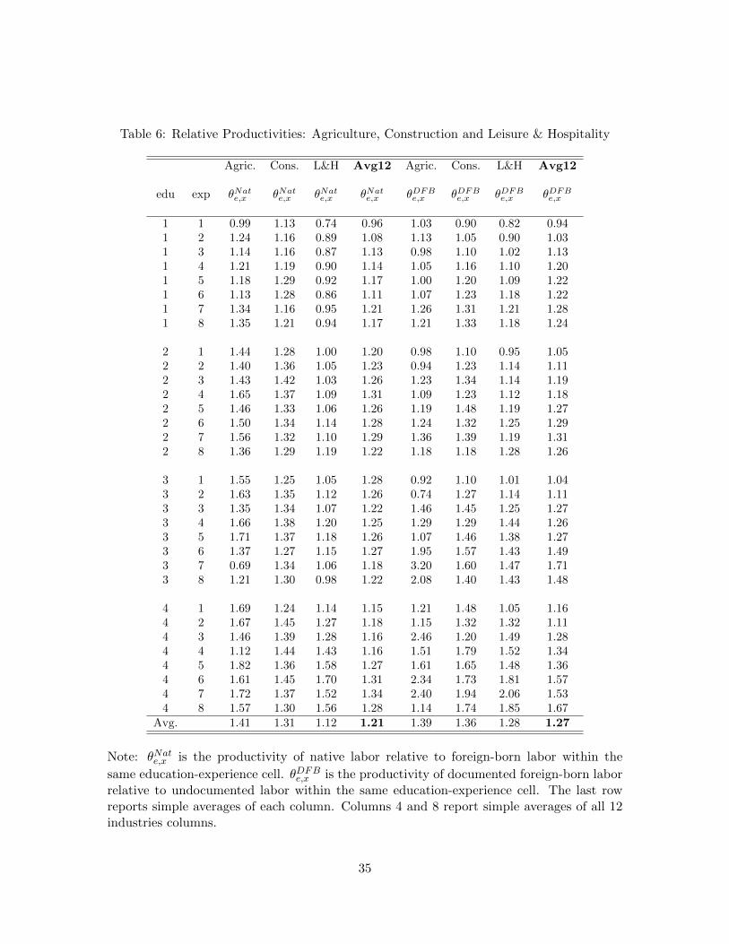
Table 6: Relative Productivities: Agriculture, Construction and Leisure & Hospitality
Agric. Cons. L&H Avg12 Agric. Cons. L&H Avg12
edu exp θNate,x θNat
e,x θNate,x θNat
e,x θDFBe,x θDFB
e,x θDFBe,x θDFB
e,x
1 1 0.99 1.13 0.74 0.96 1.03 0.90 0.82 0.941 2 1.24 1.16 0.89 1.08 1.13 1.05 0.90 1.031 3 1.14 1.16 0.87 1.13 0.98 1.10 1.02 1.131 4 1.21 1.19 0.90 1.14 1.05 1.16 1.10 1.201 5 1.18 1.29 0.92 1.17 1.00 1.20 1.09 1.221 6 1.13 1.28 0.86 1.11 1.07 1.23 1.18 1.221 7 1.34 1.16 0.95 1.21 1.26 1.31 1.21 1.281 8 1.35 1.21 0.94 1.17 1.21 1.33 1.18 1.24
2 1 1.44 1.28 1.00 1.20 0.98 1.10 0.95 1.052 2 1.40 1.36 1.05 1.23 0.94 1.23 1.14 1.112 3 1.43 1.42 1.03 1.26 1.23 1.34 1.14 1.192 4 1.65 1.37 1.09 1.31 1.09 1.23 1.12 1.182 5 1.46 1.33 1.06 1.26 1.19 1.48 1.19 1.272 6 1.50 1.34 1.14 1.28 1.24 1.32 1.25 1.292 7 1.56 1.32 1.10 1.29 1.36 1.39 1.19 1.312 8 1.36 1.29 1.19 1.22 1.18 1.18 1.28 1.26
3 1 1.55 1.25 1.05 1.28 0.92 1.10 1.01 1.043 2 1.63 1.35 1.12 1.26 0.74 1.27 1.14 1.113 3 1.35 1.34 1.07 1.22 1.46 1.45 1.25 1.273 4 1.66 1.38 1.20 1.25 1.29 1.29 1.44 1.263 5 1.71 1.37 1.18 1.26 1.07 1.46 1.38 1.273 6 1.37 1.27 1.15 1.27 1.95 1.57 1.43 1.493 7 0.69 1.34 1.06 1.18 3.20 1.60 1.47 1.713 8 1.21 1.30 0.98 1.22 2.08 1.40 1.43 1.48
4 1 1.69 1.24 1.14 1.15 1.21 1.48 1.05 1.164 2 1.67 1.45 1.27 1.18 1.15 1.32 1.32 1.114 3 1.46 1.39 1.28 1.16 2.46 1.20 1.49 1.284 4 1.12 1.44 1.43 1.16 1.51 1.79 1.52 1.344 5 1.82 1.36 1.58 1.27 1.61 1.65 1.48 1.364 6 1.61 1.45 1.70 1.31 2.34 1.73 1.81 1.574 7 1.72 1.37 1.52 1.34 2.40 1.94 2.06 1.534 8 1.57 1.30 1.56 1.28 1.14 1.74 1.85 1.67
Avg. 1.41 1.31 1.12 1.21 1.39 1.36 1.28 1.27
Note: θNate,x is the productivity of native labor relative to foreign-born labor within the
same education-experience cell. θDFBe,x is the productivity of documented foreign-born laborrelative to undocumented labor within the same education-experience cell. The last rowreports simple averages of each column. Columns 4 and 8 report simple averages of all 12industries columns.
35

Table 7: Relative Productivities by Education
No degree HS grad. Some College College grad.θ1 θ2 θ3 θ4
1. Agriculture, forestry, fish/hunt 1 1.67 1.63 2.632. Mining 1 1.50 1.48 2.393. Construction 1 1.91 1.96 2.424. Manufacturing 1 2.13 2.52 4.765. Wholesale and retail trade 1 2.24 2.47 4.416. Transportation and utilities 1 2.15 2.22 2.847. Information 1 3.18 4.45 7.788. Financial activities 1 2.85 3.96 9.489. Professional and business svcs 1 2.15 3.11 8.0310. Educational and health svcs 1 2.06 3.04 7.0711. Leisure and hospitality 1 1.76 2.00 3.4612. Other Services 1 1.91 1.99 2.84
Simple average 1 2.12 2.57 4.84GDP-weighted average 1 2.31 2.96 6.21
Note: All productivity terms are relative to the productivity of high-school dropouts in thesame industry.
Table 8: Labor shares across industries, 2011-2013
2011 2012 2013 Average
Private industries (1-12) 0.532 0.535 0.533 0.533
All non-defense industries (1-13) 0.572 0.571 0.569 0.571
1. Agriculture, forestry, fish/hunt 0.208 0.258 0.217 0.2282. Mining 0.224 0.244 0.234 0.2343. Construction 0.647 0.636 0.634 0.6394. Manufacturing 0.484 0.483 0.479 0.4825. Wholesale and retail trade 0.653 0.641 0.636 0.6436. Transportation and utilities 0.521 0.533 0.533 0.5297. Information 0.381 0.392 0.382 0.3858. Financial activities 0.257 0.252 0.252 0.2549. Professional and business svcs 0.728 0.738 0.752 0.73910. Educational and health svcs 0.855 0.863 0.867 0.86211. Leisure and hospitality 0.705 0.709 0.702 0.70612. Other services 0.751 0.748 0.755 0.75113. Public administration 0.792 0.785 0.783 0.787
Notes: We construct labor shares as compensation of employees divided by value added lesstaxes on production and imports less subsidies, per Figura and Ratner (2015). Underlyingstatistics are from the Bureau of Economic Analysis.
36

Tab
le9:
Bas
elin
eR
esu
lts
12
34
56
7
Em
p.
SR
Hou
rsSR
Hou
rsS
RE
mp.
LR
Hou
rsL
RH
ou
rsL
R
GD
P20
13Y/Y
Y/Y
Y−Y
Y/Y
Y/Y
Y−Y
1.A
gric
ult
ure
,fo
rest
ry,
fish
/hu
nt
225.
440.
979
0.98
0-4
.60.
910
0.914
-19.4
2.M
inin
g44
1.05
0.99
30.
993
-2.9
0.97
10.
972
-12.3
3.C
onst
ruct
ion
619.
870.
948
0.95
0-3
0.9
0.92
00.
923
-47.6
4.M
anu
fact
uri
ng
2024
.65
0.98
10.
982
-35.
80.
962
0.964
-73.8
5.W
hol
esal
ean
dre
tail
trad
e19
69.8
0.97
90.
979
-41.
80.
968
0.967
-64.9
6.T
ran
spor
tati
onan
du
tili
ties
754.
070.
988
0.98
8-9
.30.
977
0.977
-17.5
7.In
form
atio
n79
3.82
0.99
20.
992
-6.7
0.97
80.
978
-17.5
8.F
inan
cial
acti
vit
ies
3295
.46
0.99
60.
996
-13.
70.
983
0.984
-54.3
9.P
rofe
ssio
nal
and
bu
sin
ess
svcs
1952
.48
0.97
30.
986
-26.
70.
963
0.982
-36.1
10.
Ed
uca
tion
alan
dh
ealt
hsv
cs13
73.2
20.
989
0.98
9-1
4.7
0.98
80.
988
-17.0
11.
Lei
sure
and
hos
pit
alit
y62
5.66
0.94
40.
938
-38.
50.
922
0.914
-53.6
12.
Oth
erS
ervic
es36
3.09
0.95
90.
958
-15.
40.
945
0.944
-20.4
Tot
al14
438.
610.
983
-241
.00.
970
-434.4
$B
illi
on$
Bil
lion
$B
illi
on
Not
es:
Col
um
n1
rep
orts
the
actu
alin
du
stry
GD
Pin
year
2013
.C
olu
mn
s2-
4re
por
tth
esh
ort-
run
resu
lts.
Colu
mn
s2
and
3re
por
tth
era
tio
ofth
eco
unte
rfac
tual
indu
stry
GD
P(Y
)to
the
bas
elin
eva
lue
(Y).
Th
efo
rmer
mea
sure
sla
bor
usi
ng
emp
loym
ent
and
the
latt
eru
ses
hou
rsw
orke
d.
Col
um
n4
rep
orts
the
dol
lar
valu
eof
the
shor
t-ru
neff
ects
onin
dust
ryG
DP
base
don
the
hou
rsw
orke
dm
easu
rem
ent.
Col
um
ns
5-7
are
anal
ogou
sto
colu
mn
s2-
4b
ut
refe
rto
the
lon
g-ru
neff
ects
.T
he
short
an
dlo
ng-r
un
per
cent
chan
ges
inth
eS
um
row
are
calc
ula
ted
by
div
idin
gth
ed
olla
ram
ounts
($24
1.0
and
$434
.4)
by
pri
vate
-sec
tor
GD
Pin
2013
($14
,438
.6b
illi
on.)
37

Tab
le10
:R
obu
stn
ess.
Lon
g-ru
neff
ects
Sce
nar
io0
01
12
23
3
σe
33
33
33
33
σx
66
66
66
66
σn
2020
2020
1000
1000
20
20
σd
1000
1000
2020
1000
1000
1000
1000
Θca
lib
rati
onca
lib
rati
onca
lib
rati
onca
lib
rati
onca
lib
rati
onca
lib
rati
on
11
Y/Y
Y−Y
Y/Y
Y−Y
Y/Y
Y−Y
Y/Y
Y−Y
Bil
lion
s$
Bil
lion
s$
Bil
lion
s$
Bil
lion
s$
1.A
gric
ult
ure
,fo
rest
ry,
fish
/hu
nt
0.91
-19.
40.
91-2
0.5
0.91
-20.5
0.8
2-4
0.6
2.M
inin
g0.
97-1
2.3
0.97
-13.
50.
97-1
2.7
0.9
7-1
3.2
3.C
onst
ruct
ion
0.92
-47.
60.
92-5
0.7
0.92
-48.6
0.8
6-8
6.8
4.M
anufa
ctu
rin
g0.
96-7
3.8
0.96
-81.
20.
96-7
4.7
0.9
3-1
41.7
5.W
hol
esal
ean
dre
tail
trad
e0.
97-6
4.9
0.96
-71.
70.
97-6
5.4
0.9
5-9
8.5
6.T
ran
spor
tati
onan
du
tili
ties
0.98
-17.
50.
97-1
9.6
0.98
-17.7
0.9
6-3
0.2
7.In
form
atio
n0.
98-1
7.5
0.98
-19.
70.
98-1
7.6
0.9
7-2
3.8
8.F
inan
cial
acti
vit
ies
0.98
-54.
30.
98-6
1.6
0.98
-54.4
0.9
7-9
8.9
9.P
rofe
ssio
nal
and
bu
sin
ess
svcs
0.98
-36.
10.
98-4
0.7
0.98
-36.2
0.9
6-7
8.1
10.
Ed
uca
tion
alan
dh
ealt
hsv
cs0.
99-1
7.0
0.99
-19.
60.
99-1
7.0
0.9
8-2
7.5
11.
Lei
sure
and
hos
pit
alit
y0.
91-5
3.6
0.91
-57.
10.
91-5
4.4
0.8
8-7
5.1
12.
Oth
erS
ervic
es0.
94-2
0.4
0.94
-22.
10.
94-2
0.7
0.9
1-3
2.7
Tot
al0.
97-4
34.4
0.97
-478
.20.
97-4
40.0
0.9
5-7
47.0
Not
es:
Inth
eb
asel
ine
scen
ario
(0)
the
elas
tici
ties
ofsu
bst
itu
tion
are
(σe,σ
x,σ
n,σ
d)
=(3,6,2
0,20
)an
dth
ety
pe
pro
du
ctiv
itie
sar
eth
ose
obta
ined
inth
eca
lib
rati
on.
Col
um
ns
1an
d2
rep
ort
the
lon
g-ru
neff
ects
for
scen
ario
0.R
elati
veto
the
base
lin
e,sc
enar
io1
assu
mes
alo
wel
asti
city
ofsu
bst
itu
tion
bet
wee
nd
ocu
men
ted
and
un
docu
men
ted
fore
ign
-bor
nw
ork
ers,
an
dth
ere
sult
sar
ere
por
ted
inco
lum
ns
3an
d4.
Rel
ativ
eto
bas
elin
e,sc
enar
io2
assu
mes
ah
igh
elas
tici
tyof
sub
stit
uti
on
bet
wee
nn
ati
vean
dfo
reig
n-b
orn
wor
kers
,an
dth
ere
sult
sar
ere
por
ted
inco
lum
ns
5an
d6.
Rel
ativ
eto
bas
elin
e,sc
enar
io3
ass
um
esth
at
all
typ
ep
rod
uct
ivit
ies
equ
alon
e,an
dth
ere
sult
sar
ere
por
ted
inco
lum
ns
7an
d8.
Th
ere
lati
veva
lues
inth
eto
tals
row
are
com
pu
ted
on
the
bas
isof
the
corr
esp
ond
ing
tota
ld
olla
ram
ount
and
pri
vate
-in
du
stry
GP
Din
year
2013
.
38

Table 11: Projected losses 2017-2026
1 2 3 4Capital adjustment None 10 years 5 years Immediate
2017 279.1 279.1 279.1 503.12018 291.1 317.1 349.5 524.72019 302.4 356.3 423.7 545.02020 314.0 398.0 503.0 566.02021 326.8 443.3 589.0 589.02022 340.3 492.0 613.4 613.42023 354.3 543.9 638.6 638.62024 368.9 599.1 664.9 664.92025 384.1 658.1 692.4 692.42026 400.1 721.1 721.1 721.1
Cumulative 2017-2026 3,361.0 4,807.9 5,474.6 6,058.1$ Billion $ Billion $ Billion $ Billion
Notes: Column 1 assumes that capital remains constant at the 2016 level, and the annualGDP loss is 1.4%. Column 4 assumes that capital fully adjusts by 2017, and the annualGDP loss is 2.6%. Columns 2 and 3 assume that capital fully adjusts in 10 and 5 years,respectively. The short and long-run GDP losses are calculated by dividing the annualdollar loss by the overall GDP in the baseline year, taking into account the 12 private-sector industries and the public sector.
39

Table 12: Employment by state of residence, nativity and documentation status, 2011–2013
Emp Pct Pct Emp Pct Pctin foreign Pct Mex & in foreign Pct Mex &
State 000’s born undoc undoc State 000’s born undoc undoc
AL 2,000 4.8 2.1 1.5 MT 476 1.9 0.2 0.0AK 354 9.1 1.4 0.1 NE 963 7.4 2.8 1.8AZ 2,752 17.1 5.5 4.7 NV 1,240 25.9 8.7 6.1AR 1,246 6.5 2.7 1.9 NH 691 6.4 0.9 0.1CA 16,888 35.4 10.2 6.9 NJ 4,225 28.0 7.4 1.5CO 2,562 12.1 4.2 3.3 NM 873 12.6 4.5 4.0CT 1,768 17.4 4.6 0.8 NY 9,142 28.1 6.2 1.4DE 423 11.5 3.2 1.5 NC 4,293 10.7 4.9 3.1DC 324 18.2 3.5 0.2 ND 379 2.8 0.3 0.0FL 8,321 25.2 5.6 1.4 OH 5,297 4.8 1.0 0.4GA 4,291 13.7 5.3 3.1 OK 1,709 7.8 3.5 2.8HI 645 22.8 3.8 0.2 OR 1,751 13.2 4.4 3.5ID 707 8.0 3.1 2.7 PA 5,938 7.4 1.5 0.4IL 6,034 18.1 5.8 4.1 RI 517 15.8 3.6 0.3IN 2,997 5.8 2.1 1.4 SC 2,027 6.7 2.8 1.8IA 1,556 5.6 1.8 1.0 SD 424 3.1 0.8 0.3KS 1,395 8.5 3.3 2.3 TN 2,830 6.5 2.5 1.5KY 1,865 4.4 1.3 0.8 TX 11,817 21.8 8.7 6.5LA 2,000 5.4 1.9 0.8 UT 1,302 11.4 4.5 3.3ME 643 3.5 0.2 0.0 VT 327 4.6 0.6 0.1MD 2,960 18.7 5.4 0.6 VA 3,946 15.6 4.5 0.8MA 3,342 18.4 3.0 0.1 WA 3,202 17.2 4.9 3.1MI 4,279 7.3 1.3 0.5 WV 755 1.7 0.2 0.1MN 2,792 8.8 2.1 1.0 WI 2,839 5.6 1.8 1.4MS 1,195 3.0 1.1 0.6 WY 292 3.3 1.2 1.0MO 2,774 5.0 1.3 0.6 USA 143,369 16.9 4.9 2.7
Notes: Statistics are averages across the 2011, 2012, and 2013 waves of the augmentedAmerican Community Survey (ACS) files supplied by Center for Migration Studies (2014)and described by Warren (2014). They are drawn from the employment sample describedin the text.
40
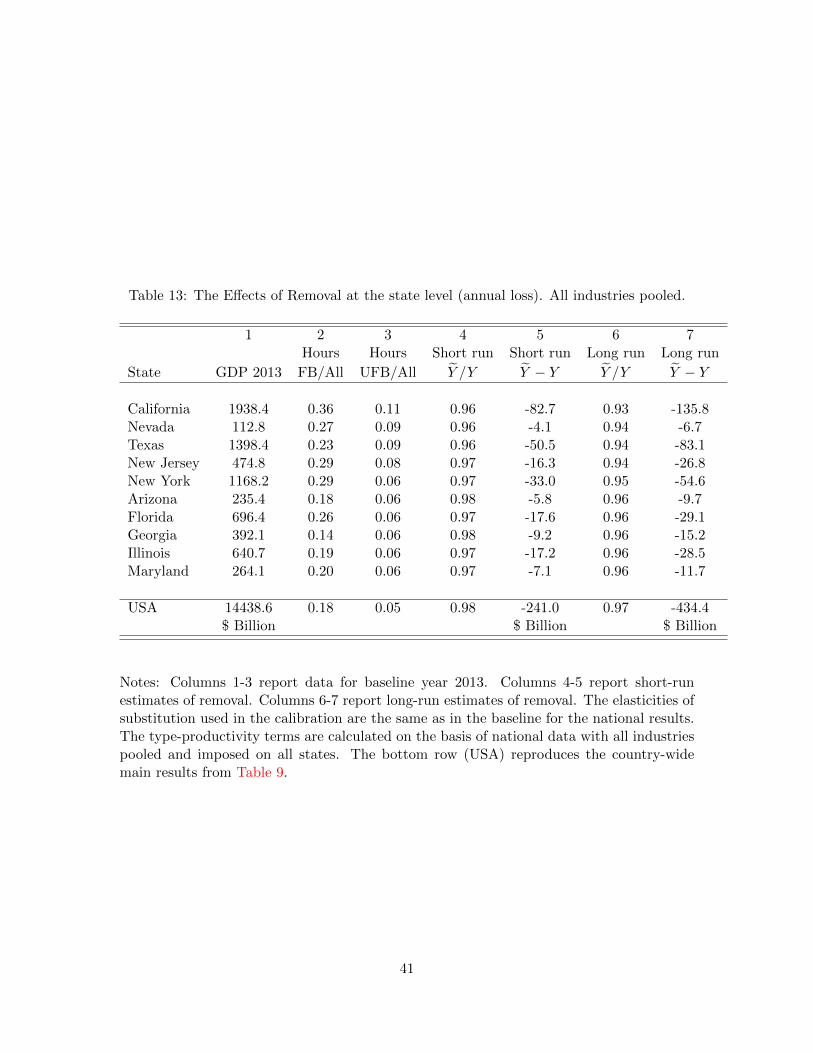
Table 13: The Effects of Removal at the state level (annual loss). All industries pooled.
1 2 3 4 5 6 7Hours Hours Short run Short run Long run Long run
State GDP 2013 FB/All UFB/All Y /Y Y − Y Y /Y Y − Y
California 1938.4 0.36 0.11 0.96 -82.7 0.93 -135.8Nevada 112.8 0.27 0.09 0.96 -4.1 0.94 -6.7Texas 1398.4 0.23 0.09 0.96 -50.5 0.94 -83.1New Jersey 474.8 0.29 0.08 0.97 -16.3 0.94 -26.8New York 1168.2 0.29 0.06 0.97 -33.0 0.95 -54.6Arizona 235.4 0.18 0.06 0.98 -5.8 0.96 -9.7Florida 696.4 0.26 0.06 0.97 -17.6 0.96 -29.1Georgia 392.1 0.14 0.06 0.98 -9.2 0.96 -15.2Illinois 640.7 0.19 0.06 0.97 -17.2 0.96 -28.5Maryland 264.1 0.20 0.06 0.97 -7.1 0.96 -11.7
USA 14438.6 0.18 0.05 0.98 -241.0 0.97 -434.4$ Billion $ Billion $ Billion
Notes: Columns 1-3 report data for baseline year 2013. Columns 4-5 report short-runestimates of removal. Columns 6-7 report long-run estimates of removal. The elasticities ofsubstitution used in the calibration are the same as in the baseline for the national results.The type-productivity terms are calculated on the basis of national data with all industriespooled and imposed on all states. The bottom row (USA) reproduces the country-widemain results from Table 9.
41

Table 14: Legalization
Short run Short run Long run Long runBillions $ Billions $
Y /Y Y − Y Y /Y Y − Y
1. Agriculture, forestry, fish/hunt 1.003 0.6 1.011 2.52. Mining 1.001 0.6 1.006 2.53. Construction 1.012 7.7 1.019 12.14. Manufacturing 1.003 6.4 1.007 13.35. Wholesale and retail trade 1.004 7.9 1.006 12.36. Transportation and utilities 1.003 2.0 1.005 3.87. Information 1.001 0.6 1.002 1.78. Financial activities 1.001 1.9 1.002 7.59. Professional and business svcs 1.003 5.5 1.004 7.510. Educational and health svcs 1.004 5.8 1.005 6.711. Leisure and hospitality 1.011 6.6 1.015 9.312. Other Services 1.005 1.7 1.006 2.2
Total 1.003 47.2 1.006 81.5
Notes: Columns 1 and 2 report the ratio of the short-run counterfactual GDP after legal-ization to actual GDP in the industry in 2013, measuring the workforce in terms of hoursworked. Columns 3 and 4 are analogous but the numerator refers to the long-run counter-factual. The relative values in the totals row are computed on the basis of the dollar gainsand GDP in the baseline year.
42

Figure 1: CES Nesting Labor Aggregate
Characteristics:
0
1: Education
2: Experience
3: U.S. Foreign born
4: Documented
NoDegree
HighSchool
SomeCollege
CollegeDegree
[1-5] [6-10] [11-15] [16-20] [21-25] [26-30] [31-35] [36-40]
Natives Foreign-born
Documented Undocumented
Notes: Adapted from Ottaviano and Peri (2012).
43