Embed Size (px)
Citation preview

The Economic and Market Value of
Coasts and Estuaries: What’s At Stake?
Edited by Linwood H. Pendleton
Produced by Restore America's Estuaries

This project was made possible through funding provided by the National Oceanic and Atmospheric Administration, Minerals Management Service, The McKnight Foundation, Shell-World Sponsor of America’s Wetland: Campaign to Save Coastal Louisiana, and National Wildlife Federation.
For more information contact: Restore America’s Estuaries 2020 N. 14th St., Ste. 210 Arlington, VA 22201
(703) 524-0248 www.estuaries.org

The Economic and Market Value of Coasts and Estuaries: What’s At Stake?
i
Foreword ....................................................................................................................................................... 1
Chapter 1 – Understanding the Economics of the Coast: An Introduction to this Volume ................... 4
It’s All About Values (Economic Values, That Is)...................................................................................... 4
Economic Value vs. Economic Impact ....................................................................................................... 9
The Chapters That Follow ....................................................................................................................... 10 References ........................................................................................................................ 11
Chapter 2 – Accounting for Ecosystem Goods and Services in Coastal Estuaries................................ 14
Introduction.............................................................................................................................................. 14
Classifying Ecosystem Goods and Services Provided by Estuaries ......................................................... 15 Figure 1: Millennium Ecosystem Assessment Categorization of Ecosystem Goods and Services ................................................................................................................................. 15
Table 1: Supporting Services Provided by Estuaries ................................................................. 16 Table 2: Regulating Services Provided by Estuaries ................................................................. 17 Table 3: Provisioning Services Provided by Estuaries .............................................................. 18 Table 4: Cultural Services Provided by Estuaries...................................................................... 19
Providing Ecosystem Goods and Services through Estuary Restoration................................................. 19 Figure 2: Total Economic Value of Estuarine Goods and Services* .................................... 22
State of the Art and Science: Case Study Examples ................................................................................. 22 The Barataria-Terrebonne Estuary ...................................................................................................... 23
Figure 3: The Barataria-Terrebonne Estuary System*.......................................................... 24 The Peconic Estuary............................................................................................................................ 26
Figure 4: The Peconic Estuary Watershed and Surrounding System.................................... 27
Future Research Needs ............................................................................................................................ 29 Figure 5: Valuation Data Distributed by Ecosystem Service ................................................ 30 Figure 6: Valuation Data Distributed by Cover Type ........................................................... 31 Figure 7: Valuation Data Distributed by Region................................................................... 31
Conclusions.............................................................................................................................................. 32 References ........................................................................................................................ 33
Chapter 3 – The Value of Estuary Regions in the U.S. Economy ........................................................... 37
Foundations of Analysis: Definitions and Data ....................................................................................... 38 Figure 1: Estuary Regions of the Continental United States ................................................ 38
Table 1: Estuary Regions, Region Groups, and States.............................................................. 39 Table 2: U.S. Department of Agriculture Urban Influence Codes: 2003.................................. 40 Table 3: Ocean Industries defined by the National Ocean Economics Program ...................... 41
Previous Studies....................................................................................................................................... 42
Size: How Do We Measure the Size of Regional Economies? ................................................................. 42 Table 4: Estuary Economies in 2004 ........................................................................................ 43 Table 5: Proportion of State Economy in Estuary Regions ...................................................... 45 Table 6: Proportion of Estuary Region in Each State ............................................................... 46
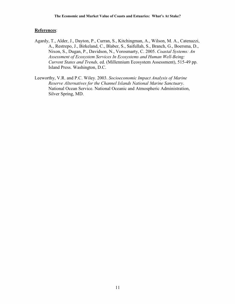
Change: What Is Changing in Regional Economies, and At What Rates? .............................................. 47 Table 7: Economic Growth in Estuary Regions 1997-2004 .................................................... 48 Table 8: Employment Growth /Population Growth Ratio by Estuary Region.......................... 50 Table 9: Change in Urban Influence Classification 1993-2003 ................................................ 52 Table 10: Employment and Population Growth by Metro/Nonmetro....................................... 54 Table 11: Population and Employment Growth by Urban Influence Type............................... 55

The Economic and Market Value of Coasts and Estuaries: What’s At Stake?
ii
How Is Change Occurring in Estuary-Dependent Sectors Compared with Overall Rates of Change?... 59 Table 12: Tourism and Recreation Growth Compared with Overall Growth ........................... 60 Table 13: Tourism and Recreation as Percent of Economy and Growth 1990-2003 ................ 61
Applying Economic Analysis at the Local Level ...................................................................................... 62
Conclusion ............................................................................................................................................... 63 References ........................................................................................................................ 64
Chapter 4 – Estuarine Restoration and Commercial Fisheries .............................................................. 65
Background – Estuaries and Their Importance for Commercial Fishing................................................ 65
Trends in Estuarine-Dependent Harvests ................................................................................................ 66
Economics of Estuarine Restoration and Commercial Fishing ............................................................... 67
Estuarine Conditions and Supply of Commercial Fisheries .................................................................... 67
Estuarine Conditions and the Seafood Consumer.................................................................................... 69
Estimating Economic Impacts of Changes in Estuarine Condition on Commercial Fisheries ................ 70
Case Study – Estuarine Water Quality Conditions and Blue Crab Harvests........................................... 71
Measuring the Commercial Fishing Benefits of Estuarine Restoration – Meeting the Challenge........... 73 Literature Cited ................................................................................................................ 74
Table 1: 2004 Landings and Value of Top Estuarine Dependent Species Compared to Total Harvest by State and Region...................................................................................................... 76
Figure 1: The Value of the Top Estuarine Dependent Species Was 38% of fhe Total U.S. Harvest in 2004 ..................................................................................................................... 77 Figure 2: Chesapeake Bay Striped Bass Harvest, 1960–2004.............................................. 77 Figure 3: Total U.S. Commercial Landings and Top Estuarine-Dependent Species, 1985–2004 ...................................................................................................................................... 78 Figure 4: Value of Total U.S. Commercial Landings and Top Estuarine-Dependent Species, 1985–2004............................................................................................................................. 78 Figure 5: Estuarine Conditions Are Reflected in the Supply Curves for Fisheries Production (Si = impaired, Sb = baseline, and Sr = restored). ................................................................. 79 Figure 6: Changes in Consumer Surplus under Varying Estuarine Conditions when Demand (D) Is Unaffected by Estuarine Conditions (Si = impaired, Sb = baseline, and Sr = restored)............................................................................................................................................... 79 Figure 7: Changes in Consumer Surplus under Varying Estuarine Conditions when Demand (Di = impaired, Db = baseline) Also Shifts with Environmental Quality (Si = impaired, Sb = baseline, and Sr = restored). .................................................................................................. 80 Figure 8: Dissolved Oxygen Levels in Different Years in Three Chesapeake Bay Tributaries During Months of Blue Crab Trotlining ............................................................................... 80 Figure 9: The Relationship Between Average Dissolved Oxygen Levels in Chesapeake Bay Tributaries and the Percentage of Stock Harvested by a Fixed (Sample Average) Amount of Trotline Gear ......................................................................................................................... 81
Chapter 5 – Determining the Economic Value of Coastal Preservation and Restoration on Critical
Energy Infrastructure ................................................................................................................................ 82
Introduction.............................................................................................................................................. 82
Perceived Conflicts Between Energy Production and Coastal Areas ...................................................... 83
Potential Synergies between Coastal Restoration and Energy Infrastructure ......................................... 84
Existing Literature on Coastal Restoration and Infrastructure Hardening ............................................. 85 Table 1: Richardson/Scott Estimated Economic Impacts, Short Oil Supply Outage (3 weeks)85

The Economic and Market Value of Coasts and Estuaries: What’s At Stake?
iii
Table 2: Richardson/Scott Estimated Economic Impacts, Short Natural Gas Supply Outage (3 weeks) ........................................................................................................................................ 85
Research Overview, Methods, and Results .............................................................................................. 86 Figure 1: Historic and Projected Land Loss......................................................................... 88 Figure 2: Potential At-Risk Energy Infrastructure ............................................................... 89 Figure 3: Storm Surge and Flooding Post-Katrina at Petrochemical Facility ....................... 90 Figure 4: Storm Surge Areas, Hurricanes Katrina and Rita ................................................. 91 Figure 5: Infrastructure in Hurricanes Katrina and Rita Inundation Zones.......................... 92 Figure 6: Potential At-Risk Infrastructure............................................................................ 92 Figure 7: Causes of Coastal Pipeline Ruptures, Historical and Projected Land Loss .......... 93
Conclusions.............................................................................................................................................. 94 References ........................................................................................................................ 95
Chapter 6 – Economic Benefits of Coastal Restoration to the Marine Transportation Sector............ 97
Introduction.............................................................................................................................................. 97
U.S. Marine Transportation Sector.......................................................................................................... 97
Links between Ports and the Environment ............................................................................................... 99
A Framework for Estimating Restoration Benefits ................................................................................ 101
Conclusions............................................................................................................................................ 103 References ...................................................................................................................... 104
Table 1: Leading Exporters and Importers in World Merchandise Trade, 2004..................... 107 Table 2: U.S. International Merchandise Trade by Mode of Transportation, 2001 ................. 107 Table 3: U.S. Waterborne Foreign Trade by Region, 2003 ..................................................... 108 Table 4: U.S. Waterborne Foreign Trade by State, 2003......................................................... 109 Source: USDOT (2006).Table 5: Major U.S. Ports by Value of Cargo, 2003......................... 109 Table 5: Major U.S. Ports by Value of Cargo, 2003................................................................ 110 Table 6: Major U.S. Ports by Weight of Cargo, 2004.............................................................. 111 Table 7: U.S. Merchant Fleet, 2004......................................................................................... 112 Table 8: U.S. Marine Industry Sector Output and Employment, 2003 .................................... 112 Table 9: Hurricane Katrina Damage Estimates for Louisiana’s Public Ports .......................... 112 Source: AAPA (2005).Table 10: Dredging Costs for FY 2005 ............................................... 112 Table 10: Dredging Costs for FY 2005.................................................................................... 113
Figure 1: Benefits from Coastal Restoration to Marine Transportation.............................. 113 Figure 2: Benefit Estimation: Natural Disasters.................................................................. 114 Figure 3: Benefit Estimation: Maintenance Dredging......................................................... 114
Case Study: Soil Erosion in the Maumee River Basin and Dredging in Toledo Harbor ................... 115 Table 11: Annual Costs with and without Sediment Reduction .............................................. 115
Reference........................................................................................................................ 115
Chapter 7 – The Influence of Coastal Preservation and Restoration on Coastal Real Estate Values116
Introduction............................................................................................................................................ 116
Water and Property................................................................................................................................ 117
A Survey of the Literature ...................................................................................................................... 118
Case Studies from the Literature............................................................................................................ 119 Studies Using Hedonic and Conjoint Choice Methods to Determine the Importance of Water Quality to Property Prices .............................................................................................................................. 119
A. Leggett and Bockstael.............................................................................................................. 119 B. St. Mary’s River Watershed.................................................................................................... 120 C. Waukegan Harbor .................................................................................................................... 121
Studies Linking Other Water Bodies and Amenities to Property Values .......................................... 123

The Economic and Market Value of Coasts and Estuaries: What’s At Stake?
iv
A. Linking Risk and Insurance Rates to Property Values............................................................. 123 B. Estimated Premium Value of Waterfront Location or Water Views for a Range of Salt and Fresh Water Bodies (surrogates, assuming that estuaries are waterfront or nearly so)................. 124
Table 1: Summary of the literature findings ............................................................................ 126
Suggestions for Further Research.......................................................................................................... 128 References ...................................................................................................................... 131
Chapter 8 – The Economic Value of Coastal and Estuary Recreation ................................................ 140
Introduction............................................................................................................................................ 140
The Economic Value of Coastal Recreation: What’s at Stake? ............................................................. 142
Coastal and Estuary Recreation in the United States ............................................................................ 143 Table 1: Coastal Recreation by State ...................................................................................... 145
The Economic Value of Coastal Recreation........................................................................................... 145 Building a Baseline of Economic Value............................................................................................ 145 Understanding and Estimating Recreational Values ......................................................................... 146
Figure 1: Activity Days as a Function of Accessing the Coast .......................................... 147 Figure 2: The Marginal Willingness to Pay for an Activity................................................ 148
Using Values from the Literature: Benefits Transfer and Value Ranges ............................................... 149 Benefits Transfer ............................................................................................................................... 149 Benefits Ranges................................................................................................................................. 150
Estimating a Baseline of Value .............................................................................................................. 150
Coastal Recreation................................................................................................................................. 150 Beach-Going...................................................................................................................................... 151
Table 2: Number of Annual Activity Days (millions) for Beach-Related Recreation in the United States (1999–2000) ...................................................................................................... 152 Table 3: Literature Review of Coastal Beach Visitation Studies for the United States .......... 153 Table 4: Estimated Annual Statewide Values of Beach-Going in the United States ($US millions)................................................................................................................................... 155
Recreational Fishing.......................................................................................................................... 156 Table 5: Literature Review of Coastal Recreational Fishing Studies for the United States.... 156 Table 6: Estimated Annual Statewide Values of Coastal and Estuary Recreational Fishing in the United States ($US millions) ............................................................................................. 159
Birdwatching and Whale Watching................................................................................................... 159 Table 7: Literature Review of Coastal and Marine Wildlife Viewing Studies for the United States........................................................................................................................................ 160 Table 8: Estimated Annual Statewide Values of Marine Wildlife Viewing (based on birdwatching activity) in the United States ($US millions) ..................................................... 161
Scuba Diving and Snorkeling............................................................................................................ 161 Table 9: Literature Review of Coastal Scuba Diving Studies for the United States ................ 162 Table 10: Estimated Annual Statewide Values of Scuba Diving in the United States ($US millions)................................................................................................................................... 163 Table 11: Literature Review of Coastal Snorkeling Studies for the United States .................. 164 Table 12: Estimated Annual Statewide Values of Snorkeling in the United States ($US millions)................................................................................................................................... 164
Coastal Recreation Is Valuable. So What? ............................................................................................ 164 Table 13: Estimated Annual Value of Select Coastal Activities in the United States............. 165
Recreational Use Value and Habitat Restoration.................................................................................. 166 Table 14: Links Between Environmental Conditions and Coastal Recreation ........................ 167
CASE STUDY: Economic Value in the Sunshine State .................................................................. 167 Table 15: Annual Participation in Coastal Recreational Activities in Florida ......................... 168 (1999/2000).............................................................................................................................. 168

The Economic and Market Value of Coasts and Estuaries: What’s At Stake?
v
Table 16: The Potential Range of Economic Use Values for the Florida Coast ...................... 168 References ...................................................................................................................... 169
The Economic and Market Value of Coasts and Estuaries: What’s At Stake?
1
The Economic and Market Value of America’s
Coasts and Estuaries: What’s At Stake
Foreword “America’s oceans and coasts are priceless assets. Indispensable to life itself, they also contribute significantly to our prosperity and overall quality of life. Too often, however, we take these gifts for granted, underestimating their value and ignoring our impact on them.” An Ocean Blueprint for the 21st Century: Final Report of the U.S. Commission on Ocean Policy,
Recognizing Ocean Assets and Challenges, page 1.
Our nation was built from the coast. The original colonies were founded on the coast. The Louisiana Purchase wasn’t just the largest land deal of its time, it was the largest transfer of wetland acreage in history. Americans, like people around the world, are drawn to the coast because of its beauty and productivity, and because our coasts are gateways to the world. The coast nurtures our frontier spirit, our need for outdoor recreation, and the constant American appetite for sweeping ocean views and quiet bayfront vistas. Because much of the American coast is made up of shifting sands or craggy cliffs, our use of the coasts historically has been concentrated in estuaries—the bays, coves, and river mouths where access is easy and safe harbor can be found. These areas are also special because of their biological importance to the nation. These estuaries, where freshwater meets the sea, are a fundamental cornerstone of ocean fisheries and aquaculture. Estuaries also generate oxygen, sequester carbon dioxide, and provide habitat to plants and animals, both marine and terrestrial. Unfortunately, we have a poor record of caring for our coasts and oceans. Years of badly planned coastal development have led to heroic, and sometimes desperate, measures to hold back the forces of nature by using engineering might rather than ecological stewardship. Seawalls have transformed once natural coasts into marine hazards unfit for the basic activities that first drew homeowners to the sea—swimming, boating, and fishing. Estuaries also have been under siege. Seen by many as bottomless pits where we can dump society’s refuse, estuaries have been poisoned across the country. Bays once filled with fish and oysters have become dead zones filled with excess nutrients, chemical wastes, and harmful algae. Wetlands, especially coastal salt marshes, have faired no better. When Mark Twain said “land was something they aren’t making any more of,” he probably never thought his country would begin a systematic program of filling coastal wetlands to create new waterfront property. But that is exactly what happened. Worse yet, coastal wetlands that were not filled were

The Economic and Market Value of Coasts and Estuaries: What’s At Stake?
2
often dredged for harbors and marinas. The result has been a loss of more than half of the nations wetlands over the past 200 years1. The damage and destruction borne by our coasts and estuaries has created more than physical and biological losses for our country. This damage also has diminished the economic productivity of the nation and the economic wellbeing of the millions of Americans who visit, use, and depend on the coast and the goods and services it provides. New efforts to protect restore America’s estuaries and coasts are likely to recapture much of this lost economic value and, in some cases, improve the economic importance of these areas to levels not see in generations. In this book, we examine the economic value of our coasts and estuaries with an eye to understanding the economic benefits of protecting and restoring America’s coasts and estuaries. The economic potential and value of the coast is richer and more complex than most people realize. Coasts and estuaries generate both economic value and economic impact—an important subtlety often overlooked in coastal development and planning. Coasts generate goods and services that are consumed through extraction (e.g., seafood); values that are never extracted, such as scenic views; and gases, such as oxygen, that are consumed globally. Understanding, accounting for, and estimating the many potential economic benefits of coastal and estuarine protection and restoration is no small feat. In this book, we introduce some of the critical concepts needed to begin to understand the economic importance of restoration. In Chapter 1, we introduce the basic economics tools, ideas, and methods used to value and quantify the economic contribution of coasts. (Readers with advanced knowledge of economics can skip this chapter.) In Chapter 2, Matthew Wilson and Stephen Farber develop an overarching framework of the economic goods and services provided by coasts and estuaries. This framework provides a way for readers to navigate the complexity of the economic system supported by coasts and helps identify those components of restoration that may generate the most substantial economic value. Protecting and restoring our coasts requires a hands-on, “boots on the ground” approach to guarding and even resurrecting the value that lies within our coasts and estuaries. In the remaining chapters, an expert panel of authors takes an appropriately hands-on approach to understanding the economic activity and value generated by key sectors of U.S. coasts and estuaries. Healthy coasts support jobs and wages, and improve housing values. Estuaries continue to be important producers of seafood and are the hubs of the nation’s international trade. Coasts provide recreational opportunities for nearly half of all Americans, generating tens of billions of dollars of economic value—far more value than is commonly recognized. Coasts also are home to a large share of the nation’s energy refining and distribution infrastructure. The health of coastal ecosystems, especially coastal wetlands, directly affects the economic vitality and resilience of the U.S. gas and petroleum industry.
1 http://www.nmfs.noaa.gov/habitat/habitatprotection/wetlands/index2c.htm

The Economic and Market Value of Coasts and Estuaries: What’s At Stake?
3
The chapters that follow will guide readers through the current state of the art in our understanding of the links between coastal and estuarine condition and economic activity. These chapters will also move beyond literature and theory to show the potential magnitude of economic value and activity associated with selected coastal-dependent economic activities. In every chapter, we offer real data and guidance about how to find locally relevant data that may help readers understand the value of restoration in their state, county, or bay. We also provide case studies that show how economic concepts, data, and analysis can help reveal the economic value of protecting these resources and even improving these values through restoration. We encourage you to use this book as a primer, a reference, and a launching point for your own efforts to understand the potential economic benefits of coastal restoration where you live and work. The book is the seed of a living project to provide restoration professionals with the economic information and guidance needed to design, monitor, and implement coastal and restoration projects. Updates to chapters, new chapters, and links to the types of data found in this book are available online at www.estuaries.org and www.coastalvalues.org. Best wishes, Linwood Pendleton The Ocean Foundation Restoration Economics Advisor, Restore America’s Estuaries

The Economic and Market Value of Coasts and Estuaries: What’s At Stake?
4
Chapter 1 – Understanding the Economics of the Coast: An
Introduction to this Volume
Linwood Pendleton The Ocean Foundation Coasts and estuaries affect people in many ways. The coast provides a place to live and recreate. Estuaries provide food for our growing population and shelter for boats, homes, and ports. And coasts and estuaries have direct and indirect effects on our physical, emotional, and personal wellbeing. Restoration of these coastal areas, likewise, will affect the personal and economic wellbeing of many people. Economic wellbeing means different things to different people. For some, economic wellbeing means having a good job. For others, economic wellbeing means happiness that sometimes comes at a financial cost (e.g., the cost of living near the beach). For politicians and public officials, economic wellbeing means economic activity, sustainable taxes, and funding for public projects. The quality of coastal and estuary areas and access to these areas influence all of these measures of economic wellbeing. Economics provides a framework for discussing and quantifying the effects that coasts and estuaries have on one aspect of personal wellbeing—our economic wellbeing. Unfortunately, the language of economics often is in terms we all know (value, impact, welfare), but the concepts that underlie economic terms often differ substantially from the meaning of these terms in everyday conversation. In this chapter, we provide a very brief introduction to the language and concepts of economics that every coastal professional and student needs to know to understand the economics of coasts and estuaries. The chapter is not intended as a comprehensive resource—we will point you to these resources along the way. Instead, the chapter is a quick run through the language and culture of economics. We hope you enjoy the trip.
It’s All About Values (Economic Values, That Is) Everyone thinks they understand value; value is part of everyday life. There are spiritual values, religious and moral values, good values on used cars, and the list goes on. When most people talk about the value of the coast, they might be talking about any of these values. When economists speak of values, however, the definition is much more narrow. For economists, value represents how much the use of a resource improves the economic wellbeing of one person or of society at large. For economists, economic wellbeing is an amalgam of values known as Total Economic Value (see http://www.csc.noaa.gov/coastal/economics/envvaluation.htm for a discussion of total economic value). Total economic value includes the value we place on goods that we can use directly (use value), the value we place on goods we use only indirectly (indirect use value), and even the value we place on goods we may never use (non-use value). Use value includes the value we place on fish we catch, trips to the beach, or the

The Economic and Market Value of Coasts and Estuaries: What’s At Stake?
5
ability to see wonderful seascapes and salt marshes. The coast also produces many goods and services we do not use directly, but which support the production of things we do use. For instance, estuary habitats provide a nursery for many types of the fish we eat. Salt marshes may act to reduce bacterial contamination of runoff and in doing so provide clean water for swimming and surfing; their intertidal vegetation draws carbon from the atmosphere (as carbon dioxide) and sequesters it in roots and marsh soils, reducing one of the most abundant greenhouse gases (GHG). Many people value coasts and estuaries even if they never plan to visit these places or use the goods and services they provide. Some people would pay to protect a coast and its inhabitants (say, the Big Sur Coast of California and its many otters, elephant seals, and sharks) just to know it exists. This non-use value is called an existence value. People may also be willing to pay so that they may have a future opportunity to enjoy the coast and its many benefits (option value) or so future generations have this opportunity (bequest value). More recently, the taxonomy of values we enjoy from natural environments has been refined to include even finer distinctions (Agardy et al. 2005). In Chapter 2, Wilson and Farber take this new taxonomy one step further and apply it specifically to the goods and services we derive from healthy coasts and estuaries. Of course, it is one thing to identify coastal economic values, and another thing entirely to estimate these values. As a start, economists attempt to measure economic value by estimating the maximum one would pay to use a resource minus the actual cost of providing access to that resource. Why is this a measure of economic wellbeing? Consider the vernacular meaning of “a good value,” which usually is taken to mean that you paid a lot less for something than you thought it was worth. I grew up eating crabs in the little town of Deltaville, Virginia, on the Chesapeake Bay, where a simple softshell crab sandwich cost $2.50. That was a value even then! The same softshell crab sandwich served in Norfolk, Virginia, cost $7.00. Not much of a value, but I’d still buy one every now and then. But when I moved west to California, the cheapest softshell crab you could find anywhere was a minimum of $9.00, even without the bread and mayonnaise! The high cost is understandable. These crabs have to take a long flight to end up between two pieces of white bread in southern California, and the $9.00 cost reflects other potential uses of that cargo space and jet fuel. That’s just not worth it to me and flying crabs to the West Coast to fulfill my culinary wants also does not make sense from society’s perspective. Consequently, I only eat softshell crab sandwiches when I’m back on the Chesapeake, and I still have not convinced anyone that I deserve a crab sandwich subsidy from the government. The point of this story is that, for economists, the term “value” comes from the idea of value added—the amount society benefits from something beyond what it costs society to make it, provide it, or protect it for use. Value is not the same thing as price! People buy things in the market as long as their maximum willingness to pay for that thing is greater than the private cost of that thing. Let’s say you are out to dinner with friends and you decide you want some oysters on the half shell. If oysters are $1.00 each, then you might

The Economic and Market Value of Coasts and Estuaries: What’s At Stake?
6
buy a half-dozen oysters. If you arrived and there were only one oyster, you might have been willing to pay much more than $1.00 for that oyster, maybe $6.00, especially if someone at the other table is asking about the same oyster. If there were two oysters, how much would you have paid for each, $4.00 apiece? For everything people consume, enjoy, or use in some way, there exists a relationship between the maximum amount someone would be willing to pay each time to enjoy this activity (whether it is eating an oyster or going to the beach) and the number of times they participate in this activity (say the number of oysters bought and eaten or the number of trips to the beach over the summer). Economists call the willingness to pay for one more of something the marginal willingness to pay (mWTP) and the total amount consumed or enjoyed is the quantity demanded (Q). The relationship between mWTP and Q is given by the demand function (Figure 1). We can estimate real demand functions, for oysters say, by looking at how many oysters people buy when oysters are available at different prices. (When we add this up across all oyster consumers, we get a market demand function,) Almost without exception, the more we consume of any good or activity, the less we are willing to pay for one more chance to enjoy it. At some point, you just can’t eat any more oysters! At that point your willingness to pay for another oyster is zero. Of course, oysters are not free, so we rarely have the luxury of eating until our hearts are content (also known as mWTP=$0.00). Harvesting oysters is costly. Growing oysters is often even more costly. The cost of providing additional oysters for the market climbs as the number of oysters brought to market increases (this is the marginal cost of oysters and is represented by the supply function in Figure 1). These costs reflect the real cost of getting oysters from seabed to table and include the cost of fuel, vessel maintenance, labor, inspection, transport, and delivery. In all cases, society has literally hundreds of other ways in which this kind of energy (human and petroleum) and equipment could have been used. When we apply these “factors of production” to oystering, we are taking them out of the economy. In the marketplace, the cost of these goods not only reflects the costs of production, but the economic value of these goods had they been used elsewhere in society (economists call this opportunity cost). For instance, consider that the diesel fuel an oysterman put in his boat could have been used to run a tractor to produce vegetables. This means that, from society’s point of view, the provision of oysters to the market had better generate added value. In fact, the market guarantees that oysters are only brought to market if the private value from buying and eating oysters is greater than the private cost of providing oysters. People continue to buy oysters and oyster harvesters and growers provide oysters as long as at least one person is willing to pay the costs of producing that last oyster and getting it to market. After that point, it is in no one’s interest to bring more oysters to market—consumers will not pay the increased cost, oyster producers will not sell for less, and society would be worse off if more time, energy, and money were invested in oyster production. The difference between the maximum that people would be willing to pay for something and the cost of providing that thing is what economists call “value.” In Figure 1, the demand function represents how much an individual (or society, when adding across all individuals) would be willing to pay for each unit of Q if we could somehow make them

The Economic and Market Value of Coasts and Estuaries: What’s At Stake?
7
pay for each unit as they consumed it. The area under the demand function (A+B+C) then represents the maximum amount the individual (or society) would be willing to pay for Q (if they had to pay). The supply function represents how much it costs a producer (or society, if added across all producers) to produce each unit of Q if we could somehow track the cost as production increases (we call this marginal cost or MC) and the area under this supply function (C) is the total cost of production. Following the logic we outlined above, economic value is the difference between maximum willingness to pay minus the cost of production (areas A+B). In a market where Q is sold at price P (where P* is the market price of oysters and Q* is the total amount of oysters purchased), the consumer enjoys a value equal to area A (the consumer surplus) and the producer enjoys a value equal to area B (the producer surplus, a concept very closely related to profit). Figure 1 tells us at least three important things we need to keep in mind when thinking about the coastal economy. First, spending, and thus revenues, associated with coastal economic activity sets an upper bound on producer surplus, but tells us nothing about consumer surplus and thus nothing about the economic value of an activity. Second, people place a higher value on something when they can get it cheaper or for free. Many coastal activities are available at little or no cost, especially to local users, while non-residents and tourists have to pay to travel to use these areas. As a result, these local users usually enjoy the greatest economic benefit from the provision of coastal goods and services. It also is true that many coastal economic activities that generate few revenues still generate significant economic value (e.g. birdwatching and beach-going). Third, in a well-functioning market, where producers only sell if they want to and consumers only buy if they want to, the market achieves a balance that maximizes economic value. When a market does not exist for something, however, there is no reason to believe that society will provide the best level of access or use of a resource. So when coastal goods and services fall outside of the market, we should be concerned that the access to coastal resources may not be socially optimal (and in virtually all cases is well below the social optimum.)

The Economic and Market Value of Coasts and Estuaries: What’s At Stake?
8
In practice, measuring the economic value of products is difficult, and so statistics regarding the economic value of marketable coastal goods and services are rare. Generally, economists tend to fall back on market prices and expenditures or revenues. In Figure 1, the gross revenues for oysters (known as the landed value when measured at the dock) are given by the areas B + C or P*x Q* where P* is the market price of oysters and Q* is the total amount of oysters purchased. This value is not consumer surplus (area A) nor is it the producer surplus (area B), and so these gross revenues do not tell us much about the contribution oyster production makes to the wellbeing of society. A focus on gross revenues and expenditures places a great deal of attention on coastal activities that produce marketable goods while other activities (say birdwatching or surfing) may go unquantified from an economic perspective. As a result, too much attention may be given to the provision of marketed goods on the coast and too little attention given to other, non-marketed but economically valuable activities. As we discussed before, many coastal resources that are free or available at relatively low cost may have very high value! Since expenditures are not necessarily indicative of value, development that favors marketed goods at the expense less-marketed goods may not be in the best economic interests of society. Many coastal goods and services are not marketed because they cannot be captured and sold directly in the market. Consider fishing at a public pier or swimming at a public beach. In both cases, local laws or customs may make charging for access impractical. In other cases, coastal goods and services may simply defy capture and sale—oxygen produced by the ocean, sea views, and the use of the ocean’s surface for boating and surfing. When there is no mechanism to permit the capture and sale of something, it is said to be non-exclusive. Further, in some cases a good is not marketed because it cannot
$/o
yst
er
B
A
Demand (mWTP) for oysters
Supply (MC) of oysters
C
P*
Q oysters Q*

The Economic and Market Value of Coasts and Estuaries: What’s At Stake?
9
be made “private.” When a good or service is non-exclusive and the enjoyment of that good by one person does not preclude or affect the enjoyment of that same good by someone else, we say that good is a public good. Unlike many other parts of our economy, coasts and oceans provide an unusually large number of economic goods and services that are difficult to introduce into the marketplace. In fact, many of these “difficult to market” coastal goods are entirely public in nature. As a result, a failure to understand the economic value of these goods and services would certainly impair our ability to appropriately manage the coast and ocean for the best economic outcome. In Chapter 2, Matthew Wilson and Stephen Farber provide a framework for classifying both marketed and non-marketed goods and services produced by coasts and oceans. In Chapter 8, we take a detailed look at the economic value of recreation along the coast by reviewing the literature to understand the potential consumer surplus of coastal recreational activities. The goal is to expand the reader’s understanding and appreciation for the important economic contribution of coastal goods and services that fall outside the traditional economic point of view.
Economic Value vs. Economic Impact When many people talk about economic value, they are really talking about economic impact (or economic activity). Economic impact represents how much money, jobs, and taxes are generated by an activity. For instance, gross revenues from sales of oysters support jobs and local businesses, and form the basis against which sales taxes are levied. While gross revenue does not provide any information about economic value, these figures are important because they are easily measured and provide a good starting point for understanding the economic contribution oysters make to the local economy, especially the tax base. In chapters 3, 4, 5, and 6, the authors examine the economic impacts of coastal business activity (gross domestic product), fisheries, oil production and refining, and marine transportation. Employment and wages also represent economic impacts of an activity. In some cases, local or federal agencies attempt to estimate employment and wages directly by censusing firms (visit the National Ocean Economics Program, www.OceanEconomics.org to see data on employment and wages that are derived directly from firms.) In some cases, however, such data are not available. For instance, we may be interested in knowing specifically about employment associated with only those hotels located directly on a stretch of Narragansett Bay. Federal reporting laws make revealing employment and earnings information for small areas difficult. Nevertheless, it is possible to survey local hotel visitors, estimate their spending on lodging, and from this estimate the number of jobs supported by tourist spending on local hotels (see, for instance, Leeworthy and Wiley’s 2003 estimate of employment and wages associated with the Channel Islands National Marine Sanctuary).

The Economic and Market Value of Coasts and Estuaries: What’s At Stake?
10
Economic value and economic impact cannot be compared directly. Without appropriate research, it is difficult to know how much of gross output or revenues (areas B + C or P*x Q*) can be considered economic value (areas A+B). It is always the case that the true producer surplus (area B in Figure 1) is substantially less than gross revenues (areas B + C or P*x Q* where P*), but the relationship between gross revenues and consumer surplus is unknown. Even though economic value and impact are not comparable, we often find ourselves making comparisons anyway. The reason for this is simple: much of the debate about environmental protection and management comes down to jobs and revenues vs. the environment. On the business side (including commercial fishing), our data largely are derived from measures of economic impact. On the non-commercial side, which includes many of the beneficiaries of coastal management and restoration, we measure the contribution of environmental improvement in terms of economic value (usually consumer surplus). When we compare economic impact to economic value we automatically put the non-commercial users at a distinct disadvantage against businesses—economic revenues always overstate the economic value to the producer. Nevertheless, as we see in Chapter 8, the non-commercial economic value of coastal uses can be very high. For recreational uses, Pendleton conservatively estimates that the economic value of coastal recreation in the United States is on the order of $20 billion to $60 billion annually for beach-going, angling, birdwatching, and snorkeling/diving—a figure that shows the value of these activities to U.S. residents beyond what they pay to enjoy these opportunities.
The Chapters That Follow In the chapters that follow, the authors explore both the economic value of coastal uses (Chapters 2, 7, and 8) and the economic impact and activity of certain coastal and estuarine economic sectors (Chapters 2, 3, 4, 5, and 6.) In doing so, we hope to introduce the many ways in which estuarine and coastal restoration can affect the economy. These chapters are starting points for the reader. The bibliographies serve as excellent resources for those interested in learning more about the economic and market impacts of restoration. Readers will also find detailed case studies that highlight the economic contributions of the coast, estuaries, and the restoration of these special resources.
The Economic and Market Value of Coasts and Estuaries: What’s At Stake?
11
References: Agardy, T., Alder, J., Dayton, P., Curran, S., Kitchingman, A., Wilson, M. A., Catenazzi,
A., Restrepo, J., Birkeland, C., Blaber, S., Saifullah, S., Branch, G., Boersma, D., Nixon, S., Dugan, P., Davidson, N., Vorosmarty, C. 2005. Coastal Systems: An Assessment of Ecosystem Services In Ecosystems and Human Well-Being:
Current States and Trends, ed. (Millennium Ecosystem Assessment), 515-49 pp. Island Press. Washington, D.C.
Leeworthy, V.R. and P.C. Wiley. 2003. Socioeconomic Impact Analysis of Marine
Reserve Alternatives for the Channel Islands National Marine Sanctuary. National Ocean Service. National Oceanic and Atmospheric Administration, Silver Spring, MD.

The Economic and Market Value of Coasts and Estuaries: What’s At Stake?
12
BASIC GUIDES TO ECONOMIC CONCEPTS AND METHODS
Economic Valuation of Natural Resources: A Guidebook for Coastal Resources
Policymakers
http://www.mdsg.umd.edu/programs/extension/valuation/handbook.htm
This online book is written for non-economists, addressing basic concepts of economic value and other tools often used in decision making.
Ecosystem Valuation
http://www.ecosystemvaluation.org/index.html
This website is designed for non-economists who "need answers to questions about the benefits of ecosystem conservation, preservation, or restoration and 'providing' a clear, non-technical explanation of ecosystem valuation concepts, methods, and applications."
Environmental Valuation: Principles, Techniques, and Applications
http://www.csc.noaa.gov/coastal/economics/envvaluation.htm
This is found on CSC’s website under Restoration Economics.
Ocean and Coastal Resource Management
Basic principles of economics with links to various methods can be found at: http://coastalmanagement.noaa.gov/initiatives/shoreline_eco_prin_sup.html
MARINE ECONOMIC DATA ON THE WEB
The National Ocean Economics Program
http://www.oceaneconomics.org
The NOEP provides a full range of the current and historical economic and socio-economic information available on changes and trends along the U.S. coast and in coastal waters. The site includes time-series information of economic and social indicators with clear definitions and descriptions for the coast and coastal ocean.
Non-market Literature on Coastal and Ocean Resources
This is a searchable database, with abstracts and some links to full text articles, for all known journal articles and technical reports that provide value estimates for the economic value of coastal and ocean resources in the United States. Enter this site through http://www.oceaneconomics.org, choose Non-market and then choose valuation studies.
NOAA's Coastal and Ocean Resource Economics
http://marineeconomics.noaa.gov/
CORE projects include socioeconomic monitoring in the Florida Keys National Marine Sanctuary, the first-ever nationwide estimate of participation rates in marine-related recreation activities, an extensive beach valuation effort in Southern California, and many other research activities.

The Economic and Market Value of Coasts and Estuaries: What’s At Stake?
13
Spatial Trends in Coastal Socioeconomics (STICS)
http://marineeconomics.noaa.gov/socioeconomics/
The STICS website provides socioeconomic data by coastal area or watershed, as well as access to multiple tools that can be used to customize, analyze, and generate reports based on these data across time and space.
Coastal Information Directory (CID)
http://www.csc.noaa.gov/cgi-bin/id/cid2k/cid2k.cgi?page='lrl'
CID provides access to web, library, and data resources relevant to coastal issues. The information can be browsed by library, data set, or pre-selected category.

The Economic and Market Value of Coasts and Estuaries: What’s At Stake?
14
Chapter 2 – Accounting for Ecosystem Goods and Services in
Coastal Estuaries
Matthew A. Wilson School of Business Administration and The Gund Institute for Ecological Economics, University of Vermont
Stephen Farber Graduate School of Public and International Affairs, University of Pittsburgh
Introduction Throughout history, humans have favored coastal locations as desirable places to live, work, and play. Forming a highly dynamic zone of convergence between land and sea, the coastal regions of the earth serve as unique geological, ecological, and biological domains of vital importance to a vast array of terrestrial and aquatic life (Agardy et al. 2005; UNEP 2006; Wilson et al. 2005). Given this abundance, it is perhaps not surprising that coastal estuaries have long served as a focal point for human activity on planet Earth. Early on, estuaries—bodies of water where oceans and rivers meet—served as places of relative shelter that also provided staging areas for harvesting food and fiber. As trading between human settlements developed, major ports often grew up near estuaries to offer sea-going vessels protection and provide access to the interior via freshwater river systems (e.g., London, Shanghai, Alexandria, and San Francisco). The industrial revolution increased the use of the coastal zone not only for the transport of raw materials and finished goods, but also for new uses such as water extraction and the discharge of waste. With the ascendance of late-industrial society, recreational aspects of the coastal zone have increased in importance, as inland waterways, stretches of beach, coral reefs, and rocky cliffs provide opportunities for leisure activity. Due to this rich abundance, today there are few if any coastal estuaries that have not been affected in some way by human intervention (Agardy et al. 2005; Vitousek et al. 1997; Wilson et al. 2005; Lotze et al. 2006). Just the fact that so many people live in close proximity to the coastal zone is a form of pressure on the natural structures and processes that provide the goods and services people desire. The population and development pressures that estuarine areas are now experiencing raise significant challenges for planners and decision makers. Communities must often choose between competing uses of the coastal environment and the myriad goods and services provided by healthy, functioning ecosystems. Should this shoreline be cleared and stabilized to provide new land for urban development, or should it be restored to its natural state to serve as wildlife habitat? Should that wetland be drained and converted to agriculture, or should more wetland area be created to provide water filtration services? Should this inlet be dredged and mined for the production of sand and gravel, or should it be preserved to provide natural tidal flow?

The Economic and Market Value of Coasts and Estuaries: What’s At Stake?
15
To choose from these competing options, it is important to know what ecosystem goods and services will be affected by coastal development or management and how these goods and services create value for different members of society (Farber et al. 2006). When confronting decisions that require tradeoffs between different ecosystem services, decision makers cannot escape making social choices: whenever one alternative is chosen over another, that choice indicates which alternative is deemed to be worth more than other alternatives. In this paper, we show that any effort to choose between the benefits associated with coastal estuaries should begin with a rigorous understanding of the many ecosystem goods and services that could be produced by these complex systems.
Classifying Ecosystem Goods and Services Provided by Estuaries Coastal estuaries include a variety of geophysical structures, including coastal plain estuaries (Chesapeake Bay), tectonic estuaries (San Francisco Bay), bar-built estuaries that form lagoons or bays (Barataria-Terrebonne), and fjords (Kenai). One common feature of estuaries is the presence of complex hydrodynamic and nutrient fluxes that result from the intermixing of fresh and saline waters. This intermixing creates salinity gradients that allow for the survival of a rich array of fauna and flora. The physical transport of sediments and nutrients also results in unique geophysical features such as bars, mud flats, lagoons, and wetlands that offer habitat for an extremely diverse group of organisms. Estuaries are the year-round home for many species (oysters), while other species move in and out of estuaries on a seasonal basis for reproduction and growth (salmon and shrimp). This rich array of estuarine types and associated flora and fauna provides a diverse mixture of goods and services to humans worldwide. An ecosystem service, by definition, supports “the conditions and processes through which natural ecosystems, and the species that make them up, sustain and fulfill human life” (Daily 1997). Ecosystem goods, on the other hand, represent the material products that are obtained from natural systems for human use (DeGroot et al. 2002). Ecosystem goods and services occur at multiple scales, from climate regulation and carbon sequestration at the global scale, to flood protection, water supply, soil formation, nutrient cycling, waste treatment, and pollination at the local and regional scales (DeGroot et al. 2002; Heal et al. 2005). They also span a range in the degree of direct connection to human wellbeing. Accurate definition and classification of ecosystem goods and services is an essential preliminary step in the valuation of coastal estuaries. In this paper, we adopt a modified version of the newly standardized system developed in the U.N.-sponsored Millennium Ecosystem Assessment (Millennium Ecosystem Assessment 2003) and adapt that system to a previously developed typology of ecosystem goods (DeGroot et al. 2002; Farber et al. 2006). The general categorization of goods and services adapted from the Millennium Ecosystem Assessment (2003) is reproduced below in Figure 1.
Figure 1: Millennium Ecosystem Assessment Categorization of Ecosystem Goods and
Services

The Economic and Market Value of Coasts and Estuaries: What’s At Stake?
16
In an important departure from the previous literature on ecosystem services (Costanza et al. 1997; Daily 1997), the Millennium Assessment classification introduced “supporting services” as a new classification of services provided by ecosystems. While not providing direct services themselves, this new type of service, which includes nutrient cycling and soil formation, is necessary for the production of the other three service categories: regulating services, provisioning goods and services, and cultural services. As the list suggests, there is no single category that captures the entire diversity of what functioning ecological systems provide to humans. In Tables 1 through 4, we take the Millennium Ecosystem Assessment classification system a step further, using the framework to identify specific goods and services provided by estuaries and match them with relevant ecosystem functions. The end result is a classification of different types of ecosystem estuarine structures and functions and the types of goods and services we expect to be provided by them.
Table 1: Supporting Services Provided by Estuaries
Supportive Services
Ecosystem structures and functions that are essential to the delivery of ecosystem services
Nutrient cycling Storage, processing, & acquisition of nutrients
Net Primary Productivity
Soil formation Capture of sediments and accumulation of organic matter
Formation of wetlands substrate and soils
Biological regulation and biodiversity
Species interactions, including pollination
Control of pests and diseases Reduction of herbivory Pollination of wetlands plants
Habitat The physical place where organisms reside
Refugium for resident & migratory species Spawning and nursery grounds for shrimp and other fish
Hydrological cycle Movement and storage of H2O through the biosphere
Aquifer recharge Maintain salinity gradients
RegulatingBenefits obtained from
regulation of
ecosystem processes
• climate regulation
• disease regulation
• flood regulation
ProvisioningGoods produced or
provided by
ecosystems
• food
• fresh water
• fuel wood
• genetic resources
CulturalNon-material benefits
from ecosystems
• spiritual
• recreational
• aesthetic
• inspirational
• educational
SupportingServices necessary for production of other ecosystem services
•Nutrient Cycling
• Soil Formation
• Primary production

The Economic and Market Value of Coasts and Estuaries: What’s At Stake?
17
As Table 1 shows, estuaries are complex ecological systems that provide a wide array of goods and services. For example, the nutrient cycling of estuaries provides critical supportive functions essential for the delivery of ecosystem services to humans (Lugo & Snedaker 1974). The fertility derived from nutrient cycling and the hydrological cycle in turn creates habitat that supports a vast array of fish, mammals, birds, and reptiles, many of which are important as human food sources and as cultural services, such as recreation and research (Ruitenbeek 1994). Chapter 4 addresses the effects of estuarine health on fish harvest. The accumulation of organic matter and the capture of sediments from upriver also form rich substrate and soils that are essential to agricultural production worldwide (Rivas & Cendrero 1991).
Table 2: Regulating Services Provided by Estuaries
Regulating services delivered by estuaries are especially important to humans. These services (listed in Table 2) include disturbance regulation, which involve the wind and flood protection afforded by coastal wetlands (Farber 1987). A study of Hurricane Andrew in 1993 concluded that storm surge in coastal Louisiana is reduced by 1 foot if intervening wetlands are increased 3.8–4.3 miles, depending on location (CWPRA 2006). In Chapter 5, Dismukes examines the relationship between coastal erosion and energy infrastructure in the Gulf of Mexico. Biochemical processes in estuaries also provide for the detoxification of human-based wastes that are commonly generated by coastal urbanization. Detoxification creates health benefits from direct water contact, and indirectly through food consumption (Kawabe & Oka 1996). Vegetation in some estuarine systems, such as wetlands and mangroves, provides for erosion control, reducing both the influx of sediments and coastal retreat (Tovilla-Hernandez et al. 2001). Estuaries also create their own climate conditions (wind, temperature, and moisture) which may moderate climate gradients for people living near the coast (Johnston et al. 2002).
Regulating Services
Maintenance of essential ecological processes and life support systems
Gas regulation
Regulation of the chemical composition of the atmosphere and oceans
Biotic sequestration of CO2 Vegetative absorption of VOCs
Climate regulation Regulation of local and global energy balance & hydrological cycle, and other biologically mediated climate processes.
Direct influence of land cover on temperature, precipitation, wind, humidity, etc.
Disturbance regulation Dampening of environmental fluctuations/disturbance
Storm protection (e.g., by barrier islands) Flood protection (e.g., by wetlands and forests)
Soil retention Erosion control and sediment retention
Prevention of soil loss by wind, wave action, runoff, or other removal processes from wetlands and barrier islands
Waste Assimilation
Removal or breakdown of nutrients and compounds
Pollution detoxification and sequestration Water purification

The Economic and Market Value of Coasts and Estuaries: What’s At Stake?
18
Table 3: Provisioning Services Provided by Estuaries
As discussed earlier, estuaries are exceedingly rich ecological systems, thereby providing a number of essential natural resources and raw materials that people value (Janssen & Padilla 1999; Tovilla-Hernandez et al. 2001). Provisioning services listed in Table 3 include foodstuffs such as edible plants and animals, as well as fertile arable land for producing crops and grazing domesticated animals (Johnston et al. 2001). Estuaries worldwide are also noted for providing raw materials such as lumber, fuelwood, and organic matter for building and manufacturing as well as supplying fuel and energy (Barbier 2000; Semesi 1998). Many medicinal and pest control chemicals are obtained from estuarine-dependent species and the genetic resources of estuarine species are well known (Primavera 1991). Estuaries and their associated structures, such as wetlands and mangrove forests, also provide critical filtering, retention, and storage of potable water in addition to providing a critical medium for commercial transportation.
Provisioning Services
Provision of natural resources and raw materials
Water supply
Filtering, retention, and storage of water
Provision of potable water and water purification Medium for transportation and ports Provision for irrigation and industrial use
Food Edible plants and animals Arable land
Hunting, fishing, crops, grazing, and aquaculture
Building & manufacturing Lumber, skins, plant fibers, oils, dyes, etc.
Fuel and energy Fuel wood and organic matter
Raw materials
Fodder and fertilizer Leaf litter, salt hay, excrements, etc.
Genetic resources Genetic resources Variety of gene pools in fish species
Medicinal and plant resources
Biological and chemical substances for use in agriculture and human treatment
Medicines and pest control chemicals obtained from estuarine-dependent species
Ornamental resources Resources for fashion, handicraft, jewelry, pets, worship, decoration, & souvenirs
Shells used as jewelry Dried grasses

The Economic and Market Value of Coasts and Estuaries: What’s At Stake?
19
Table 4: Cultural Services Provided by Estuaries
Finally, Table 4 shows cultural services, including recreation, which is easily measurable by the number of people using estuaries for a variety of recreational purposes (Farber 1988). The economic valuation of those services would reflect economic concepts such as willingness to pay for the recreation, or willingness to accept compensation for its loss. The enhancement of these services from restoration would have to estimate the increases in usage, but this is measurable through surveys or comparative studies of estuaries under different conditions. For example, in Chapter 8, Pendleton examines the economic value of coastal recreation. The aesthetic significance of estuaries, such as wetlands and barrier islands, may be expressed through people’s preferences for proximity to those ecological features. It may be easier, however, to directly measure the value of the service through housing market price premiums for location (Smith et al. 1991). Kildow shows in Chapter 7 how proximity to coasts and estuaries and the environmental condition of these resources influences housing values. Spiritual services may be reflected in stories and folklore in a culture that incorporates some element of estuaries in the story theme. Cajun folklore is a good example of this service in coastal Louisiana. Even estuarine-dependent cuisine can become a cultural phenomenon, as Cajun cooking illustrates.
Providing Ecosystem Goods and Services through Estuary Restoration Actively managing ecosystems for the delivery of ecosystem services focuses on the links between ecosystem functions and services. The goal is to sustain the flows of valuable services in an efficient, fair, and sustainable manner, taking into consideration the complex interactions within ecosystems and between humans and their supporting ecosystems (Farber et al. 2006). Alterations of ecosystems change the mix of services through changes in ecosystem structures/processes (Palmer et al. 2004). For instance, the level of some services may increase and others may decrease; increasing wetlands for storm protection may reduce fisheries habitats by reducing marsh/water edge, while increasing channel dredging may increase transportation pathways but may also reduce aesthetic beauty. Decisions about development in estuaries inevitably involves trade-offs between competing ecological services over time.
Cultural Services Enhance emotional, psychological and cognitive well being
Recreation Opportunities for rest and enjoyment
Eco-tourism, birdwatching, outdoor sports, beach-going, fishing, etc.
Aesthetic Enjoyment of landscape and its elements
Coastal beaches and wetlands, added value to coastal housing Clean water
Science & education Development of knowledge A “natural field laboratory” for understanding coastal biological and physical processes
Use of estuaries as motif in books, film, painting, folklore, national symbols, architecture, advertising, etc.
Spiritual & historic
Spiritual or historic information
Natural features with religious or historic values

The Economic and Market Value of Coasts and Estuaries: What’s At Stake?
20
Coastal estuaries around the world are currently undergoing significant pressures caused by human population growth (Agardy et al. 2005). Approximately 44% of the global population in 1994 lived within 150 km of a coastline (Cohen et al. 1997). Today, that trend appears to be accelerating. Already, more than half of the U.S. population lives along the coast and in coastal watersheds (Beach 2002). For example, in Chapter 3, Colgan finds that more than 43% of the nation’s population resides in counties with estuaries. Coastal states are among the nation’s fastest growing and are expected to experience most of the absolute growth in population in the decades ahead (Beatley et al. 2002). Humans are now a major agent influencing the morphology and ecology of the coastal zone, either directly by means of engineering and construction works and/or indirectly by modifying the physical, biological and chemical processes at work within the coastal system (Townend 2002). With recent events such as Hurricane Katrina, restoring coastal estuaries has increasingly been recognized as having the potential to provide significant benefits to society (Costanza et al. 2006). Cleaner drinking water, soil stabilization, buffering of hazardous waste, and the restoration of wildlife habitat are all examples of ecosystem services that might be delivered by revitalized estuarine landscapes. Actively restoring degraded or damaged coastal estuaries involves alterations of structures and processes in order to restore degraded hydrologic, physical, chemical, and biological functions (Palmer et al. 2004). These functions, such as nutrient cycling and sediment deposition, are the supporting functions for ecosystem services. Alterations in these supporting functions will change the flow of ecosystem services, possibly increasing the value of the estuary to humans. The ultimate objective of estuary restoration may be to increase the value of the estuary; but it may also be to simply replicate a more natural system. Focusing restoration on the useful services that might be derived from estuaries can be a useful and compelling perspective that engages the community, management agencies, and politicians (Farber et al. 2006). This perspective requires characterization and measurement of the changes in service flows anticipated from a contemplated restoration project. Valuation of these changes combines economic valuations of services, or “prices” ($P) with anticipated changes in the service flows (∆S) for a change in Total Economic Value equal to:
∆TEV = $P x ∆S, assuming no change in the price. This highlights the need to both evaluate changes in service flows and the economic “prices” associated with them over time due to changes in demands for these services (Wilson & Carpenter 1999). The measure of changes in service flows requires careful consideration of exactly what the service flows are. In some circumstances, it is possible to evaluate trade-offs, or prices, using dollars. Working in dollars is particularly convenient, since the types of non-ecological values that arise from activities that degrade ecosystem services are often measured in a dollars (Heal et al. 2005). These monetary valuations can be viewed as representing the willingness to pay to restore or sustain services, or willingness to accept

The Economic and Market Value of Coasts and Estuaries: What’s At Stake?
21
compensation in the absence of restoration or sustainability. However, it may not always be possible to accomplish this type of measurement, and rather than trying to force measurement into dollar units in inappropriate circumstances, non-monetary measures can be employed, such as ratings or rankings. In such cases, trade-offs can be established between services, as long as services being compared can be evaluated using consistent metrics, such as jobs, Net Primary Productivity (NPP), or Net Environmental Benefit equivalency ratings (Efroymson et al. 2004). A full suite of valuation techniques is often required to quantify the value of goods and services provided by coastal estuaries. The “total economic value” (TEV) includes values for the direct use of estuaries (such as a food source), indirect uses (such as storm protection), and non-use values (such as just knowing the estuary exists). A range of methods, developed by economists, can be used to establish this TEV (Freeman 1993). Figure 2 depicts a framework that links ecosystem structures and processes with the output of specific goods and services, which can then be assigned monetary values using the range of valuation techniques described in the literature and shown in the boxes at the bottom of the diagram (Desvouges et al. 1998; Freeman 1993; Heal et al. 2005). In narrowly economic terms, the natural assets of the coastal zone can thus yield direct (fishing) and indirect (nutrient cycling) use values as well as non-use (preservation) values of the coastal system. Once accounted for, these values can then be aggregated to estimate the total value (TEV) of the estuarine system (Anderson & Bishop 1986). For example, nutrient cycling is observable partially through the evaluation of Net Primary Productivity (NPP), which is the net production of biomass. NPP is a well-developed concept in ecology and is meaningfully measurable (Catovsky et al. 2002). The transformation of NPP into useful plant and animal forms provides the value from that supportive service. Soil formation is a supportive service that incorporates sediments, coral and skeletal remnants, and vegetative materials into wetland substrates. Wetlands creation is a measurable outcome of this process. The vegetation in coastal wetlands vegetation also provides for the regulation of important gases, such as sequestration of CO2. Sequestered gases and absorbed toxins are measurable regulating services that have economic value (van Kooten & Bulte 1999). Provisioning services may be measured and valued in non-monetary units. Genetic resources include the variety of species in an estuary and the variation in genotypes within species. This variety is measurable and has value insofar as variety provides insurance values in the face of uncertainty. For example, the seven species of Pacific salmon provide for a variety of salmon with different harvest seasons. Within a species, different populations provide genetic variety and locational variation that are important to the survival of the species. For example, NOAA (2006) has identified 15 distinct population segments of steelhead in Washington, Oregon, Idaho, and California.

The Economic and Market Value of Coasts and Estuaries: What’s At Stake?
22
Figure 2: Total Economic Value of Estuarine Goods and Services*
* Adapted from Turner (2000) and Wilson et. al. (2005). Total economic value is composed of a number of different types of market-based values, which can be determined using observable market behaviors, and nonmarket-based values associated with different goods and services provided by the estuary system. As Figure 2 suggests, a variety of methods may be necessary to capture the value of the many disparate services provided by the natural features of a complex ecological system. As most valuation research studies tend to apply a single methodology to assess the benefits associated with environmental assets, there is a risk that policy audiences may assume that one single study provides the “true value” of an entire ecological system. In this context, it is critical, therefore, that a more holistic approach be taken, emphasizing the potential relationships among economic values estimated by different analysts using different valuation techniques.
State of the Art and Science: Case Study Examples Two case studies reveal the diverse economic values of goods and services delivered by estuaries. Estuaries provide a wide range of ecosystem goods and services to people. However, because of the inherent linkages between ecological structures and processes within an estuary, it is often difficult to isolate and study the production of one ecosystem good or service without also considering the other goods and services associated with it.

The Economic and Market Value of Coasts and Estuaries: What’s At Stake?
23
Additionally, empirical valuation data for coastal estuaries often appears scattered throughout the scientific literature, are somewhat uneven in quality, address only a limited number of services, and are scattered across a variety of geographic contexts (Pendleton, et al., 2007). To address this gap in the literature, below we review economic analyses done in two different estuaries in order to exemplify work in the field as well as provide useful insights for further research. Expanding our knowledge of ecosystem goods and services covered at each site brings the resulting restoration effort closer to providing a full accounting of all the valuable goods and services associated with ecological restoration.
The Barataria-Terrebonne Estuary
The Barataria-Terrebonne Estuarine System (BTES) in coastal Louisiana lies at the foot of the world’s third largest river, the Mississippi, which drains about 40 percent of the contiguous United States, funneling millions of tons of sediments and nutrients annually through lower Louisiana. Lying just south and west of the City of New Orleans and Lake Pontchartrain, the BTES is wedged between the Mississippi and Atchafalaya rivers, comprising approximately 4.2 million acres of levees, forests swamps, marshes, islands, bays, and bayous (see Figure 3). The BTES provides habitat for millions of migratory waterfowl, a supportive function (Table 1), and provides for a commercial harvest of more than 600 million pounds of finfish and shellfish every year (a provisioning service, Table 3) (Caffey & Breaux 2005). Diverse flora and fauna and a unique combination of land and water features yield a variety of goods and services. For example, both freshwater and saltwater wetlands throughout the BTES provide prime habitat for an array of plant life such as bald cypress and swamp maple, as well as wildlife such as alligators, muskrats, egrets, and herons, which are useful commercially as well as recreationally (a cultural service, Table 4). Water stored in inland freshwater wetlands after a heavy rain is released slowly, reducing flood peaks and property damage (a regulating service, Table 2) as well as supplying aquifer recharge and drinking water to coastal communities (a supporting and provisioning service, Tables 1 and 3). Barrier islands and coastal marshes create a critical zone of friction that slows winds and waters of tropical storms and hurricanes arriving from the Gulf of Mexico (a regulating service, Table 2). The BTES provides a good example of the wide variety of ecosystem services provided by estuaries. This estuarine system supports a thriving commercial fishery and recreational activities, provides protection against coastal storms, and supports a unique Cajun culture. Farber and Costanza (1987) estimated the marginal productivity of a coastal system in Terrebonne Parrish, Louisiana, by attributing commercial values for several species to the net biomass, habitat, and waste treatment of the wetland ecosystem (Farber & Costanza 1987). Arguing that the annual harvest from an ecosystem is a function of the level of environmental quality, the authors chose to focus on the commercial harvest data for five different native species—shrimp, blue crab, oyster, menhaden, and muskrat—to estimate the marginal productivity of wetlands. The annual economic value (marginal product) of each species, adjusted to 2005 dollars using the Consumer Price Index, was as follows: shrimp $21.29/acre; blue crab $1.31/acre; oysters

The Economic and Market Value of Coasts and Estuaries: What’s At Stake?
24
$15.76/acre; menhaden $11.37/acre; and muskrat pelts $23.70/acre. Taken together, the total value marginal productivity of wetlands in Terrebonne Parish was estimated at $73.43 per acre.
Figure 3: The Barataria-Terrebonne Estuary System*
A more recent study of the economic impacts of the estuary show that hunting and trapping within the four major parishes alone contributed $137 million in spending for the economy of the region in 1994 (Industrial Economics 1996). Aquaculture accounted for $10 million, and agriculture in these parishes accounted for $180 million in spending. The levels of these provisioning (Table 3) services are highly dependent on the conditions of the estuary and its accompanying barrier islands. Shipbuilding within the estuary was responsible for $1.2 billion in spending. The viability and cost of shipbuilding would be dependent on estuarine conditions, as storm protection and the ability to move built vessels to open water are critical factors for this industry, providing regulating services (Table 2). In addition to the commercial activity that is dependent on its resources, the BTES provides area residents and visitors with a number of recreational opportunities. Recreational fishing, hunting, and wildlife viewing contributed $956 million (1994 dollars) in spending in the four-parish region (Industrial Economics 1996). These commercial and recreational industries alone were responsible for roughly 11% of the total spending in this region. In these instances the estuary has provided important natural inputs to the commercial and recreational activities. It is very important to note that spending generated from activities is not itself a measure of economic value or ecosystem services, as interpreted by economists. In the examples

The Economic and Market Value of Coasts and Estuaries: What’s At Stake?
25
above—shipbuilding, recreation, and aquaculture—spending is also the result of non-ecological services from labor, built infrastructure, etc. To understand the economic value of the ecosystem services of estuaries, we would first need to determine what difference these estuaries made to the wellbeing of people; for example, how recreational fishing contributes to the economic wellbeing of people, how much more income is generated from aquaculture due to the services of estuaries, or how much less costly shipbuilding is because of the estuaries. However, the examples are suggestive of some type of dependency of these activities on the existence and functioning of estuaries. There are additional goods and services provided by the BTES other than those that provide inputs to various commercial processes or recreational uses. For instance, the storm protection services of the wetlands in the BTES and its barrier island system, a regulatory service, are very important to the natural and built infrastructure in coastal Louisiana (Costanza et al. 2006). Significant property damages have been attributed to flooding from tidal surges and rainfall as well as wind damage associated with major storm events in the region, including Hurricane Katrina (Bohannon & Enserink 2005; Kerr 2005). For example, Farber and colleagues collected historical data on property damages associated with hurricanes that have damaged the coast of Terrebonne parish (Farber 1987; Farber & Costanza 1987). Damage estimates were derived from data provided by the U.S. Army Corps of Engineers and included both wind and flood damage. Controlling for other factors, such as population and hurricane strength, the authors estimated the increase in damages resulting from increased proximity to the landfall of a hurricane. They concluded that, if a 1-mile band of wetlands on a 250-mile-long strip of coast were to disappear, the net present value of expected damages (inflated to $2005 using the single family home construction price index) would range from $2.82 million (8% discount rate) to $9.22 million (3% discount rate). These present values can be translated into $17.46 and $58.73 per acre, respectively. In a separate analysis, Farber (1996) uses an Avoided Cost (AC) method for measuring the storm surge protection value of coastal wetlands against damage to property in coastal Louisiana. Using a cost assessment of building levees around major southern Louisiana cities in the BTES, Farber estimates the annualized costs of purchasing land, building materials, and labor as well as performing annual maintenance. The analysis assumes that annual wetland loss rates remain constant at 25,806 acres per year, and shows that the total annualized costs for levee construction have a very large range—from $69.9 million to $10.6 billion depending on assumed discount rates (original estimates inflated to $2005 using U.S. Army Corps of Engineers construction cost indices for levees and floodwalls: http://www.usace.army.mil/publications/eng-manuals/em1110-2-1304/a-a.pdf). In addition to protecting property from storms and saltwater inundation, wetlands in the BTES clean the water passing into them, removing unwanted nutrients, pathogens, and sediment (a regulating, waste assimilation service; Table 2). Various coastal municipalities have found this function to be an effective tertiary treatment for wastewater (Breaux et al. 1995; Costanza et al. 1989; Farber 1996). In a series of case studies taken from Breaux et al. (1995), Industrial Economics (1996) estimated the per-

The Economic and Market Value of Coasts and Estuaries: What’s At Stake?
26
acre value of wetlands for treating different wastewater streams in the BTES. The net present value estimates of the wastewater treatment services range widely, from $98.4 per acre for municipal water treatment to $5,551 per acre for potato chip manufacturing waste treatment (original estimates inflated to $2005 using the GDP deflator and a 3% discount rate). Taken together, the results reviewed above show that the total economic importance of the BTES cannot be captured by any single economic measure, nor have all of the possible ecosystem goods and services been monetized (see Figure 1). Using our framework for classifying ecosystem goods and services, it is clear that the estuary supports several provisioning services, including major industries such as shipbuilding and commercial fisheries that have direct and indirect impacts on the regional economy. Additionally, the estuary provides several cultural and regulating services, such as recreational opportunities, storm protection, and waste assimilation. However, we also know that the BTES provides spiritual and cultural values that are integral to Cajun culture (Caffey & Breaux 2005), and we also understand that supporting services such as soil formation from the sedimentation of the Mississippi River are critical to alleviating subsidence of communities in the region(Bohannon & Enserink 2005). Yet these monetary values remain unknown because they have not been fully analyzed in the economic literature. Given the variety of assets associated with this complex system, we therefore anticipate that several new empirical studies using different valuation techniques will be required to assess the full range of values.
The Peconic Estuary
The Peconic Estuary System (PES), situated at the East End of Long Island, New York, consists of more than 100 bays, harbors, embayments, and tributaries (Figure 3). The major river discharging freshwater into the estuary is the Peconic River. This freshwater then mixes with saltwater to form the numerous bays in the estuary leading out into the Atlantic Ocean. The area surrounding the estuary’s watershed consists of rolling farmland, scenic beaches, woodlands, and wetlands featuring numerous rare ecosystems that are home to many plant and animal species (Balla et al. 2005; Peconic Estuary Program 2001). The environmental and natural resources of the PES—the bay waters, beaches, wetlands, ecosystems, habitats, and parks and watershed lands—provide many valued goods and services to the public. Currently, the PES is in relatively good condition (Balla et al. 2005). For instance, there is “a larger percentage of undisturbed habitats and a greater diversity of natural communities within this watershed than anywhere else in the coastal zone of New York State” (Peconic Estuary Program 2001, p. 10). While excessive nutrient loading in an estuary can result in low dissolved oxygen levels (Whitehead et al. 1997), overall the PES is not currently experiencing widespread low levels of oxygen, and toxic contamination is not currently a significant problem in the estuary (Peconic Estuary Program 2001).

The Economic and Market Value of Coasts and Estuaries: What’s At Stake?
27
Figure 4: The Peconic Estuary Watershed and Surrounding System
The bay waters, nearshore eelgrass beds, and wetlands support significant stocks of fish, shellfish, birds, and other species used for water-dependent and water-related commercial activities (a provisioning service, Table 3). According to the recent Peconic Estuary Program, Comprehensive Conservation Management Plan, in 1993 more than 1,000 establishments in the PES were identified as “estuarine-dependent” and gross revenues for those establishments exceeded $450 million per year (Peconic Estuary Program 2001). The living resources of the estuary also attract visitors and residents, providing cultural, recreational, and aesthetic services (Table 4). East End towns such as Southold, Riverhead, and East Hampton are home to approximately 100,000 people year-round, and the population swells in the summer to over 280,000. While visiting the PES, visitors spend money on goods and services that contribute to the local economy. For instance, in 1995 a survey was conducted by Economic Analysis Inc. asking seasonal visitors how much they spent at roadside farmsteads and at vineyards while visiting the area (Grigalunas & Diamantedes 1996). The results reveal that in 1995 the public spent approximately $8.7 million at farm stands and $2.4 million at vineyards in PES-related activities. The PES also provides critical nursery and habitat services for fish and shellfish species that are used by commercial fisheries. In an example of coastal wetland productivity analysis, Johnston et al. (2002) used a simulation model based on biological functions that contribute to the overall productivity of the food web in the PES in Suffolk County. Based on habitat values for finfish, shellfish, birds, and waterfowl, an average annual

The Economic and Market Value of Coasts and Estuaries: What’s At Stake?
28
abundance per unit area of wetland habitat in the PES is estimated by summing all relevant food web values and habitat values for a year (Johnston et al. 2002). The value of fish and shellfish is based on commercial harvest values. The marginal value of bird species usage of the habitat is based on the benefits human receive from viewing or hunting waterfowl (recreational services). Using these values as input data, the simulation model resulted in annual values (1995 dollars) for three nearshore habitat types: eelgrass ($1,065 per acre/year); saltmarsh ($338 per acre/year); and inter-tidal mud flat ($67 per acre/year). To illustrate the range of non-market economic values associated with PES, a series of empirical studies conducted as part of the multidisciplinary Peconic Estuary Program have explored a suite of different ecosystem goods and services using a range of non-market valuation techniques(Grigalunas & Diamantedes 1996; Johnston et al. 2002; Johnston et al. 2001; Opaluch et al. 1999). For instance, open space, proximity to clean water, and scenic vistas are often cited as a cultural, aesthetic service (Table 4) that provides a primary attractor of residents who own property and live within PES. Hedonic pricing (HP) techniques have been used to show that the prices of East End housing units vary with respect to characteristics such as ambient environmental quality (i.e., proximity to shoreline, water quality) because buyers will bid up the price of units having more of a desirable attribute (Johnston et al. 2001; Opaluch et al. 1999). Principal findings of the first-stage hedonic analysis show that a parcel of land in the PES adjacent to preserved open space has, on average, a 12.8% higher per-acre value than a similar parcel located elsewhere. Among other things, the PES is very popular because of the numerous recreational opportunities, including swimming, beach use, bird and wildlife viewing, boating, and fishing (Peconic Estuary Program 2001). To capture the benefits associated with outdoor recreational uses in the PES, a Travel Cost (TC) analysis was conducted (Johnston et al. 2002; Opaluch et al. 1999). In 1995, a recreational survey was administered to residents, second homeowners, and visitors to the PES. Results reveal that in 1995, over 127,000 people took 3.3.million swimming, boating, fishing, or shellfishing outings and over 150,000 people engaged in about 5.2 million beach use, birdwatching, wildlife viewing, or hunting trips (Opaluch et al. 1999). Taken together, the annual value (original estimates are inflated to $2005 using the consumer price index) of each activity were estimated as follows: $63 million for viewing birds and wildlife, $29 million for recreational fishing, $23 million for boating, and $15 million for swimming. As noted earlier, the PES is widely recognized as a uniquely beautiful and important natural resource. To capture this value, a Contingent Valuation (CV) survey was conducted to estimate the value associated with the existence of the PES as a unique natural place (Johnston et al. 2002; Opaluch et al. 1999). The CV survey was conducted by Opalauch and his colleagues over a 6-month period in 1995 with residents and second homeowners in the PES. The focus of the survey was on the restoration and protection of five natural resources, including wetlands, shellfishing areas, and eelgrass areas. Based on responses to contingent choice questions developed by the authors, the average estimated annual per-acre dollar values (original estimates are inflated to $2005 using the

The Economic and Market Value of Coasts and Estuaries: What’s At Stake?
29
consumer price index) were $5,760 for unpolluted shellfish grounds, $6,144 for saltmarsh, and $7,680 for eelgrass beds. Aggregated over a 25-year time horizon at a 7% discount rate, the net present values per acre ranged from $39,680 to protect safe shellfishing areas to $108,800 to protect eelgrass (Opaluch et. al. 1999; p.117). Taken together, it is clear that the numerous ecological assets of the PES are enjoyed by both residents and visitors to the area. Bountiful living resources support commercial activities as well as many non-market assets. Several efforts to quantify the ecosystem goods and services associated with this unique resource have been illustrated here. However, as with the case of the BTES above, we can also see that critical supporting services such as soil formation and nutrient cycling remain un-monetized. Similarly, we might reasonably anticipate that spiritual and historical values accrue from the existence of the PES, yet these assets remain unaccounted for in the economic literature. No single methodology can capture the total asset value of the PES; rather, a combination of different methods—each designed to measure a different good or service—appears to provide an improved understanding of the values offered by the estuary.
Future Research Needs The BTES and PES studies reveal that many different landscape features and ecological processes associated with estuaries provide essential natural services to humans, but that the reporting of their economic values still remains uneven in quality and scope. For example, as the case studies show, commercial values, opportunities for recreation, and aesthetic amenities receive major attention in the economic literature. Other services, such as spiritual and historic values, soil formation, and nutrient cycling, receive less attention. While perhaps not surprising given the early development of ecological economics as a field of study, the uneven distribution of empirical analyses raises critical issues for decision makers that will need to be addressed as scholars strive to better understand the full economic benefits associated with estuary restoration. Wilson and Liu (2007) recently performed a literature search of peer-reviewed publications related to coastal ecosystem services. This search yielded more than 300 citations. Each citation was located and reviewed by the authors. About 230 citations (>77%) were rejected because they were not peer-reviewed or did not explicitly address the economic valuation of coastal ecosystem goods and services. The literature review yielded a total of 70 studies and 155 data observations for further analysis and discussion. Results from these studies were sorted by land cover type, ecosystem good and service, valuation methodology, and region of study and are presented below. The recent review of the peer-reviewed literature reveals that many different landscape features and ecological processes within the coastal and nearshore marine zone provide essential natural services to humans, but that the reporting of their economic values remains unevenly distributed (Wilson and Liu 2007; Pendleton et. al. 2007). For example, as the pattern of data in Figure 5 confirms, opportunities for recreation and natural amenities (e.g., nearshore fisheries, white sandy beaches) get an inordinate amount of attention in the economic literature, while other services such as spiritual and

The Economic and Market Value of Coasts and Estuaries: What’s At Stake?
30
historic or biological control do not get much attention at all. Similarly, as Figure 6 shows, nearshore ocean, open space, freshwater wetlands, and saltwater wetlands, marshes, or salt ponds have tended to receive the most attention in the peer-reviewed literature, while areas such as mangroves and coral reefs have received far more limited attention by economists. Finally, as Figure 7 clearly shows, the vast majority of economic valuation studies in the peer-reviewed literature have been conducted in the United States with other regions such as Europe, Australia, and New Zealand lagging behind. While perhaps not surprising given the early development of environmental and ecological economics as a field of study, the uneven distribution of empirical analyses raises critical issues for decision makers that will need to be addressed in the not-too-distant future.
Figure 5: Valuation Data Distributed by Ecosystem Service
In recent decades the field of economic valuation and environmental benefit transfer has matured into a viable approach for estimating the value of environmental goods and services (Wilson & Hoehn 2006). The international peer-reviewed literature in the field has grown substantially, and transfer methods are increasingly being recognized as distinct from those used in conventional market valuation analyses. In the maturation process, the use of ecosystem services as a distinct theoretical framework has developed, and innovative methods for measuring economic values associated with these services have emerged (Farber et al. 2006; UNEP 2006). Nevertheless, our ability to assess the total economic value of complex ecological systems such as coastal estuaries remains dependent on the quality of original benefit estimation (Desvouges et al. 1998). Total value assessment is simply not feasible when there are no original economic studies for identified ecosystem goods or services, the original studies are outdated, or they are poorly designed and reported. While the latter constraint may be theoretically obvious, it all too often limits the use of benefit transfer in practice. The lack of benefit studies across multiple contexts remains one of the significant challenges to the growth and sustainability of online databases. From a
0 20 40 60 80 100
Sources
Spritual and historic
Aethetic
Recreation
Net primary production
Water supply
Water regulation
Biological control
Distrubance regulation
Habitat

The Economic and Market Value of Coasts and Estuaries: What’s At Stake?
31
practical policy perspective, important ecological services may be neglected in policy analysis because there are simply no suitable empirical studies from which benefits may be inferred (Pendleton, et al., 2007).
Figure 6: Valuation Data Distributed by Cover Type
0 10 20 30 40
Sources
Nearshore Open Space
Nearshore Ocean--50mdepth or 100km offshore
Semi-enclosed Seas
Mangrove
Coral Reefs and Atolls
Nearshore Islands
Seagrass beds or KelpforestsNearshore FreshwaterWetlands
Saltwater Wetlands,Marshes or Salt PondsBeaches and Dunes
Estuaries and Lagoons
Figure 7: Valuation Data Distributed by Region
Creative thinking is needed to put in place the incentives that will stimulate empirical data collection to supply the raw information needed for the full assessment of benefits provided by coastal estuaries. Innovative, interdisciplinary thinking must continue be encouraged to foster the development of a comprehensive research effort—one that is coupled with methodological tools that facilitate our ability to extend ecological and economic knowledge from one context to another with minimal loss of information. The challenge is to maintain an inclusive rather than an exclusive perspective as analysts from different disciplines and professional backgrounds work together to expand our collective knowledge and understanding.
0 20 40 60 80 100 120
Sourc
es
Europe
Central and South America
North America
Australia and New Zealand
East Asia
Southeast Asia

The Economic and Market Value of Coasts and Estuaries: What’s At Stake?
32
Conclusions Ecosystem goods and services form a fundamental connective link between people and coastal estuarine systems. Accurate definition and classification of ecosystem goods and services is therefore an essential preliminary step in the valuation of coastal estuaries. In this paper, we have shown how ecosystem goods and services delivered by estuaries contribute to human welfare through both simple and complex pathways. Using an integrated framework developed for the assessment of ecosystem goods and services, we have considered how ecological structures and processes, land use decisions, and human values interact in the coastal and nearshore marine environment. The concept of ecosystem goods and services has allowed us to analyze how human beings as welfare-maximizing agents actively translate complex ecological structures and processes into value-laden entities that can be understood by people. The literature reviewed here demonstrates both the opportunities and the challenges inherent in estimating the total economic value of estuarine ecosystem goods and services. As the pattern of data in the BTES and PES case studies suggests, one of the major insights from our analysis is the discrepancy between the ecosystem goods and services that have been well-documented in the published valuation literature and those that could potentially contribute significantly to human welfare, both directly and indirectly. Accounting for “missing” economic values that have not yet been analyzed represents a significant challenge for scientists, planners, and decision makers involved in coastal zone management. Our analysis further suggests that methodological guidelines and standards for the total economic assessment of ecosystem goods and services in estuaries are still evolving. Nevertheless, it is evident that, by using the ecosystem goods and services classification framework within specific contexts, defensible dollar estimates can be obtained and thereby add to the information base for coastal management and decision making. Economic estimates may require considerable creative research and have substantial uncertainties. The best available data suggest that humans attach substantial positive values to the many marketed and non-marketed goods and services provided by estuaries. We conclude with the observation that the studies presented here represent a very small subset of estuaries in the world. Hence, our ability to generalize remains limited, but promises to grow as more environmental valuation studies are done. The observations and results presented here provide valuable insights into the challenges and limitations of ecosystem service valuation as it is currently practiced. The experiences summarized here should be useful to ecologists, managers, and social scientists as they collaborate to estimate the future direction for development in the coastal environment.

The Economic and Market Value of Coasts and Estuaries: What’s At Stake?
33
References
Anderson, G. D., Bishop, R. C. 1986. The Valuation Problem. In Natural resource
economics: policy problems and contemporary analysis, ed. (D. W. Bromley),89-137 pp. Liuwer Nijoff Publishing. Boston, MA.
Agardy, T., Alder, J., Dayton, P., Curran, S., Kitchingman, A., Wilson, M. A., Catenazzi, A., Restrepo, J., Birkeland, C., Blaber, S., Saifullah, S., Branch, G., Boersma, D., Nixon, S., Dugan, P., Davidson, N., Vorosmarty, C. 2005. Coastal Systems: An Assessment of Ecosystem Services. In Ecosystems and Human Well-Being: Current States and Trends, ed. (Millennium Ecosystem Assessment),515-49 pp. Island Press. Washington, D.C. .
Balla, R., Bavro, L., deQuillfeldt, C., Miller, S. 2005. Peconic Estuary Program Environmental Indicators Report. Peconic Estuary Program. Riverhead, NY.pp.
Barbier, E. B. 2000. Valuing the environment as input: review of applications to mangrove-fishery linkages. Ecological Economics 35: 47-61.
Beach, D. 2002. Coastal Sprawl: The Effects of Urban Design on Aquatic Ecosystems in the United States. Pew Oceans Commission. Arlington, VA.pp.
Beatley, T., Brower, D. J., Schwab, A. K. 2002. An Introduction to Coastal Zone Management. Island Press. Washington, DC.
Bohannon, J., Enserink, M. 2005. Scientists Weigh Options for Rebuilding New Orleans. Science 309: 1808-9.
Breaux, A., Farber, S., Day, J. 1995. Using Natural Coastal Wetlands Systems for Waste-Water Treatment - an Economic Benefit Analysis. Journal of Environmental Management 44: 285-91.
Caffey, R. H., Breaux, J. 2005. Portrait of an Estuary: Functions and Values of the Barataria-Terrebone Estuary System. Barataria-Terrebone National Estuary Program and Louisiana Cooperative Extension Service. Thibodaux, LA.pp.
Catovsky, S., Bradford, M. A., Hector, A. 2002. Biodiversity and ecosystem productivity: implications for carbon storage. Oikos 97: 443-8.
Cohen, J. F., Small, C., Mellinger, A., Gallup, J., Sachs, J. 1997. Estimates of Coastal Populations. Science 278: 1211-2.
Costanza, R., d'Arge, R., deGroot, R., Farber, S., Grasso, M., Hannon, b., Limburg, K., Naeem, S., O'Neill, R. V., Paruelo, J., Raskin, R. G., Sutton, P., van den Belt, M. 1997. The Value of the World's Ecosystem Services and Natural Capital. Nature 387: 253-60.
Costanza, R., Farber, S., Maxwell, J. 1989. Valuation and Management of Wetland Ecosystems. Ecological Economics 1: 335-61.
Costanza, R., Mitsch, W. J., Day, J. 2006. Creating a sustainable and desirable New Orleans. Ecological Engineering 26: 317-20.
CWPPRA, 2006. Coastal Wetlands Planning Protection and Restoration Act (CWPPRA): A Response to Louisiana’s Land Loss, A Report by the Louisiana Coastal Wetlands Conservation and Restoration Task Force.
Daily, G. C. 1997. Nature's Services: Societal Dependence on Natural Ecosystems. Island Press. Washington D.C.

The Economic and Market Value of Coasts and Estuaries: What’s At Stake?
34
DeGroot, R., Wilson, M. A., Boumans, R. M. J. 2002. A typology for the classification, description, and valuation of ecosystem functions, goods and services. Ecological Economics 41: 393-408.
Desvouges, W. H., Johnson, F. R., Banzhaf, H. S. 1998. Environmental Policy Analysis with Limited Information: Principles and Applications of the Transfer Method. Edward Elgar. Northhampton MA.
Efroymson, R. A., Nicollete, J. P., Suter, G. W. 2004. A Framework for Net Environmental Benefit Analysis for Remediation or Restoraion of Contaminated Sites. Environmental Management 34
Farber, S. 1987. The value of coastal wetlands for the protection of property against hurricane wnd damage. Journal of Environmental Economics and Management 14: 143-51.
---. 1988. The Value of Coastal Wetlands for Recreation - an Application of Travel Cost and Contingent Valuation Methodologies. Journal of Environmental Management 26: 299-312.
---. 1996. Welfare Loss of Wetlands Disentegration: A Louisiana Study. Contemporary Economic Policy 14: 92-106.
---. Costanza, R. 1987. The Economic Value of Wetlands Systems. Journal of Environmental Management 24: 41-51.
---. Costanza, R., Childers, D., Erickson, J., Gross, K., Grove, M., Hopkinson, C., Kahn, J. R., Pincetl, S., Troy, A., Warren, P., Wilson, M. A. 2006. Linking Ecology and Economics for Ecosystem Management. Bioscience 56: 117-29.
Freeman, M. 1993. The Measurement of Environmental and Resource Values. Resources for the Future. Washington D.C.
French, P. W. 1997. Coastal and Estuarine Management. Routledge. New York, NY. Grigalunas, T. A., Diamantedes, J. 1996. The Peconic Estuary System: Perspectives on
Uses, Sectors, and Economic Impacts. Economic Analysis, INC. Peace Dale, RI.pp.
Grigalunas, T. A., Opaluch, J. J., Trandafir, S. 2004. Non-Market Benefits and Costs of Preserving Estuarine Watershed Open Space: A Case Study of Riverhead, Long Island, New York., Economic Analysis Inc. December 15, 2004. Peacedale, Rhode Island.pp.
Heal, G. M., Barbier, E. B., Boyle, K. J., Covich, A. P., Gloss, S. P., Hershner, C. H., Hoehn, J. P., Pringle, C. M., Polasky, S., Segerson, K., Schrader-Frechette, K. 2005. Valuing Ecosystem Services: Toward Better Environmental Decision-Making. The National Academies Press. Washington D.C. .
Industrial Economics. 1996. Economic Value Assessment for the Barataria-Terrebone Estuarine System. Rep. BTNEP Publication #6. pp.
Janssen, R., Padilla, J. 1999. Preservation or Conversion: Valuation and Evaluation of a Mangrove Forest in the Philippines. Environmental and Resource Economics 14: 297-331.
Johnston, R. J., Grigalunas, T. A., Opaluch, J. J., Mazzotta, M., Diamantedes, J. 2002. Valuing estuarine resource services using economic and ecological models: the Peconic Estuary System study. Coastal Management 30: 47-65.
Johnston, R. J., Opaluch, J. J., Grigalunas, T. A., Mazzotta, M. J. 2001. Estimating Amenity Benefits of Coastal Farmland. Growth and Change 32: 305-25.

The Economic and Market Value of Coasts and Estuaries: What’s At Stake?
35
Kawabe, M., Oka, T. 1996. Benefit from improvement of organic contamination of Tokyo Bay. Marine Pollution Bulletin 32: 788-93.
Kerr, R. A. 2005. Is Katrina a Harbinger of Still More Powerful Hurricanes? Science 309: 1807.
Lotze, H.K., Lenihan, H.S., Bourque, B.J., Bradbury, R.H., Cooke, R.G., Kay, M.C., Kidwell, S.M., Kirby, M.X., Peterson, C.H., and Jackson, J.B.C., 2006. Depletion, Degradation, and Recovery Potential of Estuaries and Coastal Seas, Science, Vol. 312. no. 5781, pp. 1806 - 1809
Lugo, A., Snedaker, S. C. 1974. The Ecology of Mangroves. Annual Review of Ecology and Systematics 5: 39-64.
Millennium Ecosystem Assessment. 2003. Ecosystems and Human Well-Being: A Framework for Assessment. Island Press. Washington DC.
NOAA. 2006. ESA Salmon Listings. Accessed from: http://www.nwr.noaa.gov/ESA-Salmon-Listings/. On: September 12.
Opaluch, J. J., Grigalunas, T. A., Diamantedes, J., Mazzotta, M., Johnston, R. J. 1999. Recreational and Resource Economic Values for the Peconic Estuary System. Economic Analysis Inc.,. February, 1999. Peacedale, Rhode Island.pp.
Palmer, M., Bernhardt, E., Chornesky, E., Collins, S., Dobson, A., Duke, C., Gold, B., Jacobson, R., Kingsland, S., Kranz, R., Mappin, M., Martinez, M. L., Michell, F., Morse, J., Pace, M., Pascual, M., Palumbi, S., Reichman, O. J., Simons, A., Townsend, A., Turner, M. 2004. Ecology for a Crowded Planet. Science 304: 1251-2.
Peconic Estuary Program. 2001. Peconic Estuary Comprehensive Conservation and Management Plan. Suffolk County Department of Health, Program Office. Suffolk, NJ.866 pp.
Pendleton L., Atiyah, P. and A. Moorthy. 2007. Is the Non-Market Literature Adequate to Support Coastal and Marine Management? Ocean and Coastal Management (Forthcoming).
Primavera, J. H. 1991. Intensive Prawn Farming in the Philippines - Ecological, Social, and Economic-Implications. Ambio 20: 28-33.
Rivas, V., Cendrero, A. 1991. Use of Natural and Artificial Accretion on the North Coast of Spain - Historical Trends and Assessment of Some Environmental and Economic Consequences. Journal of Coastal Research 7: 491-507.
Rosenberger, R. S., Loomis, J. B. 2000. Using meta-analysis for benefit transfer: In-sample convergent validity tests of an outdoor recreaton database. Water Resources Research 36: 1097-107.
Ruitenbeek, H. J. 1994. Modeling Economy Ecology Linkages in Mangroves - Economic Evidence for Promoting Conservation in Bintuni Bay, Indonesia. Ecological Economics 10: 233-47.
Semesi, A. K. 1998. Mangrove management and utilization in Eastern Africa. Ambio 27: 620-6.
Smith, V. K. 1992. On separating defensible benefit transfers from 'smoke and mirrors'. Water Resources Research 28: 685-94.
Smith, V. K., Palmquist, R. B., Jakus, P. 1991. Combining Farrell Frontier and Hedonic Travel Cost Models for Valuing Estuarine Quality. The Review of Economics and Statistics 73: 694-9.

The Economic and Market Value of Coasts and Estuaries: What’s At Stake?
36
Tovilla-Hernandez, C., de la Lanza, G. E., Orihuela-Belmonte, D. E. 2001. Impact of logging on a mangrove swamp in South Mexico: Cost/benefit analysis. Revista De Biologia Tropical 49: 571-80.
Townend, I. 2002. Marine Science for strategic planning and management: the requirement for estuaries. Marine Policy (In Press)
UNEP. 2006. Marine and coastal ecosystems and human well-being: A synthesis report based on the findings of the Millennium Ecosystem Assessment. UNEP. New York.1-76 pp.
van Kooten, G. C., Bulte, E. H. 1999. How much primary coastal temperate rain forest should society retain? Carbon uptake, recreation, and other values. Canadian Journal of Forest Research-Revue Canadienne De Recherche Forestiere 29: 1879-89.
Vitousek, P. M., Mooney, H. A., Lubchenco, J., Melillo, J. M. 1997. Human Domination of Earth's Ecosystems. Science 227: 494-9.
Whitehead, J. C., Hoban, T. L., Clifford, W. B. 1997. Economic analysis of an estuarine quality improvement program: The Albemarle-Pamlico system. Coastal Management 25: 43-57.
Wilson, M. A., Carpenter, S. R. 1999. Economic Valuation of Freshwater Ecosystem Services in the United States 1971-1997. Ecological Applications 9: 772-83.
Wilson, M. A., Costanza, R., Boumans, R. M. J., Liu, S. L. 2005. Intergrated Assessment and Valuation of Ecosystem Goods and Services Provided by Coastal Systems. In The Intertidal Ecosystem, ed. (James G. Wilson),1-24 pp. Royal Irish Academy Press. Dublin, Ireland.
Wilson, M. A., Hoehn, J. P., eds. 2006. Special Issue--Environmental Benefits Transfer: Methods, Applications and New Directions. Ecological Economics. Forthcoming, Nov-Dec.
Wilson, Matthew A. and Liu, Shuang. 2007. Evaluating the Non-Market Value of Ecosystem
Goods and Services provided by Coastal and Nearshore Marine System. In M. Pattterson and B. Glavovic (eds.) Ecological Economics of the Oceans and Coasts. Edward Elgar. Northampton, MA. (In Review).

The Economic and Market Value of Coasts and Estuaries: What’s At Stake?
37
Chapter 3 – The Value of Estuary Regions in the U.S.
Economy
Charles S. Colgan University of Southern Maine The deteriorating condition of the nation’s critical estuary habitats is well-documented.1 The need to restore estuaries to their previously high level of natural functioning and the means to achieve restoration also are well-understood. The causes of estuarine degradation are many and varied, but primarily arise from differing types of economic activities. Despite the negative consequences of economic activity on estuarine health, the economic importance of healthy estuarine habitat is ubiquitous in all discussions of plans for estuarine habitat restoration. A strong connection between economic activity and the case for estuarine habitat restoration is widely acknowledged, but the explicit links between economic activity and estuarine health are not well developed and rarely exploited by policy makers. This paper examines the role of the nation’s estuary regions in generating economic activity that contributes to the total value of goods and services in the United States and as sources of livelihoods in order to assess what, in very general terms, is at stake in decisions about efforts to preserve and restore estuarine resources. The predominant focus in this paper is on the measurement of total economic activity in estuarine regions. Other papers in this series examine the specific dimensions of activities, such as ports and fisheries, that are obviously directly connected to estuaries. Understanding these direct connections is important, but ports, energy, real estate development, and fisheries are in turn connected to a complex network of other activities that together comprise the regional economy. The analysis of specific sectors of economic activity is the beginning of the process of measuring the economic value of estuaries; the full picture requires an understanding of both the details of estuarine-dependent sectors and their connections to the larger economies in which these sectors function. To see this larger picture, this chapter explores the nature of the economies of estuarine regions from several different perspectives:
• Size: how do we measure the size of regional economies in which estuaries are located?
• What is changing in the economy of estuary regions, at what rates, and how do the changes define the context within which estuary restoration takes place?
• Where is change occurring in the estuary region?
• How is change occurring in estuary-dependent sectors compared with overall rates of change?
1 A National Strategy to Restore Coastal and Estuarine Habitat (Restore America's Estuaries 2002)

The Economic and Market Value of Coasts and Estuaries: What’s At Stake?
38
To address these questions, we use a quasi-national perspective, focusing on the economies of the estuary regions of the lower 48 states. The regions chosen are those defined and discussed in the National Strategy for the “lower 48” states. The unique geographies of Alaska and Hawaii complicate the discussion, so these states are omitted, though the principles of economic analysis developed here can certainly be applied to these states as well. The picture that emerges from this analysis is far from complete or adequate for people in specific regions who are trying to decide how to proceed with decisions about specific restoration projects. For that reason, the concluding section of the paper points to resources where data is available for readers wishing to understand their own regional economy.
Foundations of Analysis: Definitions and Data
We begin the development of our framework by setting out measures of economic activity. As noted above, we assess these measures in terms of the major estuary regions of the United States, based on the regions defined in A National Strategy to Restore Coastal and Estuarine Habitat (Restore America's Estuaries 2002). These regions are, in one sense, larger than the areas usually encompassed by specific estuarine restoration projects. But the data presented here allows an economic dimension to be added to the details about estuary restoration in the national strategy, and serves to illustrate basic principles of economic measurement and analysis that can be useful at any geographic level.
Figure 1: Estuary Regions of the Continental United States
Puget Sound
Ore-Wash Coast
No. Calif
So. Calif
Western Gulf
Central Gulf
Eastern Gulf
Southern Gulf
Florida Atlantic
Georgia South Carolina
North Carolina
Chesapeake Bay
Delaware River
N.Y Bight
Gulf of Maine
Lake Ontario
Lake Erie
Lake Huron
Lake Michigan
Lake Superior

The Economic and Market Value of Coasts and Estuaries: What’s At Stake?
39
Table 1: Estuary Regions, Region Groups, and States
Group Region States
Gulf of Maine Maine, New Hampshire, Massachusetts
N Y Bight Rhode Island, Connecticut, New York, New Jersey
Delaware River New Jersey, Pennsylvania, Delaware
Northeast Atlantic
Chesapeake Bay Pennsylvania, Maryland, District of Columbia, Virginia
North Carolina North Carolina
South Carolina South Carolina, North Carolina
Georgia Georgia
Southeast Atlantic
Florida Atlantic Florida
Southern Gulf Florida
Eastern Gulf Florida, Alabama
Central Gulf Mississippi, Louisiana, Texas
Gulf of Mexico
Western Gulf Texas
Northern California California California
Southern California California
Oregon-Washington Coast Oregon, Washington
Pacific Northwest
Puget Sound Washington
Lake Erie New York, Pennsylvania, Ohio, Michigan
Lake Ontario New York
Lake Michigan Michigan, Indiana, Illinois, Wisconsin
Lake Huron Michigan
Great Lakes
Lake Superior Michigan, Wisconsin, Minnesota
These broadly defined estuary regions encompass a variety of terrain and ecosystems, as well as a variety of socioeconomic characteristics. One key socioeconomic dimension is the distinction between urban areas and rural areas, which roughly measures the intensity of land use. The standard method for doing this is to distinguish between metropolitan and nonmetropolitan areas, which are designated according to data based on the decennial census from the Office of Management and Budget. While useful, the metro-nonmetro distinction does not contain a great deal of information. A more useful taxonomy is provided by the Urban Influence Codes developed by the U.S. Department of Agriculture, primarily for the purpose of understanding key characteristics of rural (nonmetropolitan) areas.
The urban influence codes extend the metro-nonmetro distinction by looking at the size of the largest central place (city or town) in the county and, for nonmetro areas, whether a county is adjacent to a metro area. Population size of the most densely settled place and the relative location of each county within the region compared to the most densely settled place thus can be incorporated into the taxonomy. For rural areas, the question of adjacency to a metro area is a particularly important factor, since a metro area’s

The Economic and Market Value of Coasts and Estuaries: What’s At Stake?
40
economic influence can extend well beyond its borders. Measuring change using this approach allows an analysis of the spread of economic activity across the landscape as an indicator of potential impacts on estuaries. The Urban Influence Codes are shown in Table 2.
Table 2: U.S. Department of Agriculture Urban Influence Codes: 2003
Central Place
Population Location Relative to
Metro Area
1 million or greater
250,000 to 1 million
Metro
Less than 250,000
Adjacent to Metro Area 20,000 or greater
Not adjacent to Metro Area
Adjacent to Metro Area 2,500 to 19,000 Not adjacent to Metro
Area
Adjacent to Metro Area
Nonmetro
Less than 2,500 Not adjacent to Metro Area
For this analysis, the socioeconomic measures to be used are population, employment, and output.
• Population change is the most commonly used measure of socioeconomic change in regions, but it is primarily a measure of longer-term change. Population changes relatively slowly, and does not easily pick up shorter-term fluctuations in economic activity.
• Employment data are the most consistently measured data on economic activity at the regional level. Employment is measured in different ways, such as by place of employment and by place of employee’s residence. It is measured across the country for most industries on a monthly basis, and time series of the data can be constructed in some cases for more than 30 years.
• Output is a measure of what is produced in the economy. The statistic used is the gross domestic product (GDP) or the state-level version, the gross domestic product-state (GDP-S). These measures are estimated on a “value added” basis. That is, they avoid double counting the production of one industry that is also the input to another industry. For example, the output of commercial fishing does not equal the sum of the sales of the fish harvester to the processor plus the sales of the processor to the supermarket. Rather, the correct measure is the value added

The Economic and Market Value of Coasts and Estuaries: What’s At Stake?
41
by the harvester in catching the fish, by the processor in transforming the fish into a salable product, and by the market in displaying the fish for the consumer (and perhaps by the restaurant for preparing the fish and by trucking companies for moving the fish between various stages).
The organizing taxonomies to be used are the “coastal economy” and the “ocean economy.” These concepts were developed for the National Ocean Economics Program (NOEP) and are fully described in A Guide to the Measurement of the Market Data for the Ocean and Coastal Economy in the National Ocean Economics Program available at www.oceaneconomics.org. This data is the outgrowth of research describing the economic activity associated with coastal and ocean areas going back more than 30 years. This research is briefly summarized in the section on literature below.
The NOEP data used for this analysis include total employment and output for all sectors in each estuary region to gauge the total magnitude of economic activity. In addition, the NOEP data allow for analysis of specific industries. These industries are shown in Table 3. This chapter includes an analysis of tourism and recreation, a key estuary-dependent sector. The analysis in this paper complements the discussion of the economic value of recreation in the accompanying chapter by Pendleton.
Table 3: Ocean Industries defined by the National Ocean Economics Program
Construction – Marine Tourism & Recreation
Marine-related Construction Amusement and Recreation Services, NEC*
Living Resources – Marine Boat Dealers
Fishing Eating & Drinking Places
Fish Hatcheries and Aquaculture Hotels & Lodging Places
Seafood Processing Marinas
Seafood Markets Recreational Vehicle Parks & Campgrounds
Minerals – Offshore Scenic Water Tours
Limestone, Sand, & Gravel Sporting Goods Retailers
Oil and Gas Exploration Zoos, Aquaria
Oil and Gas Production Transportation – Marine
Deep Sea Freight Transportation
Marine Passenger Transportation
Ship & Boat Building Marine Transportation Services
Boat Building and Repair Search and Navigation Equipment
Ship Building and Repair Warehousing
* Not elsewhere classified
The identification of economic activity as part of the ocean economy depends in part on the industry, as defined under the North American Industrial Classification System, and in part on location. For a list of the specific industries and NAICS codes, see the NOEP Users Guide. Certain establishments (places of business) are defined as part of the ocean economy when they are located near the shoreline (in this case, by location in a shore-adjacent zip code). In Table 3, these industries are shown in italics.

The Economic and Market Value of Coasts and Estuaries: What’s At Stake?
42
Previous Studies
Previous studies of the economy of the estuary region and estuary-related industries have been defined not in terms of estuaries as the key geographic feature but in terms of coasts and oceans. The first attempt at measuring economic activity related to the oceans attempted to estimate an “ocean GDP” from a national perspective. In 1974, the Bureau of Economic Analysis (the agency responsible for maintaining the National Income and Product Accounts) engaged a consultant to undertake a special study for the Assistant Secretary of Commerce for Policy to identify the contribution of the ocean to the GNP (Nathan Associates 1974). In that study, the BEA developed estimates for Gross Product Originating from the Ocean-Related Activities using the Economic Census data for 1972. Two follow-up studies used a similar approach to estimate the values for 1977 and 1987 (Pontecorvo, Wilkinson et al. 1980; Pontecorvo 1988). Following studies on the national ocean economy, attention turned to the coastal economy. Luger developed a methodology for measuring coast-dependent, coast-linked, and coastal-service activities (Luger 1991). This approach significantly expanded the types of economic activities brought into the measurement process. By focusing on the coastal zone, Luger also brought the Great Lakes into the analysis, since they are defined for federal management purposes as part of the coastal zone. Another group of studies on the economic value of the oceans has focused on the economy of various regions as influenced by the oceans. Some of these studies have been done at the state level (Moeller and Fitz 1994) (Kildow, Colgan et al. 2005), while others have been done at the multi-state and international level (Colgan and Plumstead 1993) (Statistics New Zealand, 2006). Studies of the Ocean Economy in Canadian provinces also have been undertaken (Mandale, Foster et al. 1998; Mandale, Foster et al. 2000). These studies have tended to rely on employment in specific industries or estimates of output from regional econometric models, and have thus focused on the market-related activities that are the most easily measured.
These various studies were the foundations on which the data series used by the National Ocean Economics Program and used in this paper were developed. The NOEP approach derives measurements of the coastal and ocean economies using the most detailed records available. The result is a nationally consistent data set from the county level to the national level that provides both detail on key sectors and the flexibility to define regions in different ways. The NOEP data also provides sub-state estimates of GDP for the ocean and coastal economies, which are not available in any other federal data sets. For more information see (Colgan 2006).
Size: How Do We Measure the Size of Regional Economies?
Table 4 presents data on the population, employment, and gross domestic product (GDP) from each of the continental U.S. estuary regions in 2004. The actual magnitudes are given for each region, along with the proportion of the U.S. total population,

The Economic and Market Value of Coasts and Estuaries: What’s At Stake?
43
employment, and GDP. The subtotals of each estuary region group are shown, along with the totals of all estuary regions.
Table 4: Estuary Economies in 2004
Population % of US Employment Percent of US
GDP (Millions of $) % of US
Gulf of Maine 7,301,185 2.5% 3,572,361 2.6% $354,857 3.0% NY Bight 25,249,074 8.5% 10,891,224 7.8% $1,286,113 11.0%
Delaware River 6,630,623 2.2% 3,047,511 2.2% $318,250 2.7%
Chesapeake Bay 5,188,369 1.7% 3,228,576 2.3% $301,864 2.6%
Total North
Atlantic 44,369,251 15.0% 20739672 14.9% $2,261,085 19.4%
North Carolina 1,907,423 0.6% 733,567 0.5% $52,257 0.4%
South Carolina 1,875,763 0.6% 727,957 0.5% $52,027 0.4% Georgia 799,620 0.3% 308,606 0.2% $22,016 0.2%
Florida Atlantic 8,003,332 2.7% 3,237,208 2.3% $294,639 2.5%
Total
South Atlantic 12,586,138 4.2% 5007338 3.6% $420,940 3.6%
Southern Gulf 1,402,660 0.5% 547,810 0.4% $44,501 0.4% Eastern Gulf 4,704,515 1.6% 1,932,458 1.4% $155,228 1.3% Central Gulf 8,993,578 3.0% 3,921,796 2.8% $398,241 3.4% Western Gulf 1,169,069 0.4% 394,376 0.3% $30,974 0.3%
Total Gulf of
Mexico 16,269,822 5.5% 6796440 4.9% $628,943 5.4%
Southern California 16,630,780 5.6% 7,072,280 5.1% $735,681 6.3% Northern California 10,592,542 3.6% 4,744,068 3.4% $567,543 4.9% Oregon-Washington Coast 2,610,431 0.9% 735,572 0.8% $148,200 0.9% Puget Sound 3,864,854 1.3% 1,803,453 1.3% $186,581 1.6%
Total Pacific 33,698,607 11.4% 14796252 10.7% $1,594,630 13.7%
Lake Ontario 1,260,578 0.4% 544,919 0.4% $44,812 0.4% Lake Erie 7,541,639 2.5% 3,288,116 2.4% $288,103 2.5% Lake Huron 551,184 0.2% 196,339 0.1% $13,864 0.1%
Lake Michigan 9,843,927 3.3% 4,491,371 3.2% $440,784 3.8%
Lake Superior 488,609 0.2% 201,897 0.1% $13,458 0.1%
Total
Great Lakes 19,685,937 6.6% 8722642 6.3% $801,022 6.9%
Total All
Estuary Regions 126,609,755 42.7% 56,062,344 40.4% 5,706,619 49.0%
It is apparent that the estuary regions comprise a very significant portion of the total United States economy. The estuary regions make up about 12.6% of the area of the

The Economic and Market Value of Coasts and Estuaries: What’s At Stake?
44
continental United States, but on that relatively small area can be found nearly 43% of the U.S. population, about 40% of employment, and almost half (49%) of the output of the U.S. economy.
The North Atlantic region (Maine through Virginia) is the largest of the major regions, with 15% of population and employment and 20% of output. This is because the region includes the New York Bight estuary region, which runs from Long Island Sound to the Delaware River and borders the New York metropolitan area. The two California regions (Southern and Northern) are next largest after the New York Bight, followed by Lake Michigan. The smallest regions are Lake Huron and Lake Superior.
Another indicator of the economic importance of estuary regions is a comparison of the relative proportions of population and GDP in each region. A region whose share of the national economy exceeds its share of national employment serves as an “economic center.” A region such as this produces, on average, more output per worker than other regions where the share of employment is larger than that of output. By this standard, all of the North Atlantic estuary regions plus all of the Pacific estuary regions qualify as economic centers, as do the Florida Atlantic, Central Gulf of Mexico, Lake Erie, and Lake Michigan regions.
The proportion of the national economy found in estuary regions provides one perspective on the size of these areas. Another is to be found by examining the relative size of the economic activity in a state’s estuary counties (those counties comprising the estuary regions) as a proportion of the state’s total economy. Thus, one might ask: what proportion of each state’s economy is to be found in the estuary counties in that state? This question is addressed in Table 5. Each state is shown, along with the population, employment, and output to be found in all counties identified as part of an estuary region. The table also shows, for each state, which estuary regions or portions of estuary regions are found in that state. Connecticut, Delaware, and Rhode Island are the three states in which the economy is entirely within the estuary regions. States with over 90% of their economy (measured by GDP) in estuary regions include Maine, Massachusetts, and New Jersey. States with between 80% and 90% include California and Louisiana. Florida and Washington State have almost at 80% of their economy in the estuary regions.2
2 Florida’s political and estuarine geographies create some artificial distinctions when the county boundaries are used. It may be plausibly argued that all of Florida is within an estuary region, including the central Florida counties excluded in this analysis.

The Economic and Market Value of Coasts and Estuaries: What’s At Stake?
45
Table 5: Proportion of State Economy in Estuary Regions
State Name
Population in Estuary Region(s)
% of State Population in Estuary Regions(s)
Employment in Estuary Region(s)
% of State Employment
in Estuary Region(s)
GDP in Estuary
Region(s)
% of State
GDP in Estuary
Region(s)
Estuary Region(s)
included in state
Alabama 726,338 16.1% 268,219 14.8% $19,035 13.5% Eastern Gulf
Southern Calif. California 27,223,322 76.0% 11,816,348 80.7% $1,303,224 85.8%
Northern Calif.
Connecticut 3,498,966 100.0% 1,583,549 100.0% $182,468 100.0% N.Y. Bight
Delaware 830,069 100.0% 406,260 100.0% $52,298 100.0% Delaware River
Florida Atlantic
Southern Gulf Florida 13,328,406 76.7% 5,432,923 76.2% $474,240 77.8%
Eastern Gulf
Georgia 855,383 9.6% 324,940 8.6% $23,109 6.8% Georgia
Illinois 6,020,034 47.4% 2,819,551 50.5% $306,575 57.4% Lake Michigan
Indiana 754,656 12.1% 23,732 0.9% $23,732 10.3% Lake Michigan
Louisiana 3,575,024 79.3% 1,511,068 81.2% $133,058 83.1% Central Gulf
Massachusetts 5,587,689 87.2% 2,761,203 88.9% $287,347 91.9% Gulf of Maine
Maryland 2,262,404 46.0% 1,271,922 52.6% $115,658 50.1% Chesapeake Bay
Maine 1,224,242 93.1% 552,632 93.9% $41,092 95.0% Gulf of Maine
Lake Michigan
Lake Huron Michigan 5,044,878 49.9% 1,911,168 45.7% $167,156 45.6%
Lake Erie
Minnesota 214,615 4.2% 100,464 3.9% $7,230 3.2% Lake Superior
Mississippi 606,962 20.9% 210,443 19.9% $15,262 19.8% Central Gulf
North Carolina North Carolina
2,046,672 24.0% 490,480 11.9% $43,449 13.4% South Carolina
New Hampshire
1,062,219 81.8% 774,342 20.8% $55,130 17.0% Gulf of Maine
N.Y. Bight New Jersey 8,293,936 95.5% 3,664,133 96.6% $397,808 97.0%
Delaware River
N.Y. Bight
Lake Ontario New York 16,316,589 84.6% 6,930,262 85.2% $407,189 44.9%
Lake Erie
Ohio 2,766,162 24.2% 1,359,914 25.9% $115,825 27.2% Lake Erie
Oregon 2,114,503 29.4% 1,003,214 58.4% $91,240 67.8% Ore-Wash Coast
Delaware River
Lake Erie Pennsylvania 5,432,681 43.8% 2,569,193 47.4% $243,279 52.5%
Chesapeake Bay
Rhode Island 1,079,916 100.0% 467,533 100.0% $41,844 100.0% N.Y. Bight
South Carolina
1,736,514 41.4% 687,182 39.7% $49,155 37.4% South Carolina
Western Gulf Texas 5,980,661 26.6% 2,594,661 28.1% $280,895 31.1%
Central Gulf
Virginia 1,375,597 18.4% 1,308,706 38.1% $136,735 41.8% Chesapeake Bay
Puget Sound Washington 4,360,782 70.3% 1,976,690 73.5% $200,166 79.1%
Ore-Wash Coast
Lake Michigan Wisconsin 82,545 1.5% 976,667 36.6% $81,290 39.1%
Lake Superior

The Economic and Market Value of Coasts and Estuaries: What’s At Stake?
46
Table 6: Proportion of Estuary Region in Each State
Estuary Region
States Included Population
% of Estuary Region Employment
% of Estuary Region
GDP (Millions)
% of Estuary Region
LA 3,575,024 39.8% 1,511,068 38.5% $133,058 33.4%
MS 606,962 6.7% 210,443 5.4% $15,262 3.8% Central Gulf
TX 4,811,592 53.5% 2,200,285 56.1% $249,921 62.8%
MD 2,262,404 43.6% 1,271,922 39.4% $115,658 38.3%
PA 1,550,368 29.9% 647,948 20.1% $49,471 16.4% Chesapeake Bay
VA 1,375,597 26.5% 1,308,706 40.5% $136,735 45.3%
DE 830,069 12.5% 406,260 13.3% $52,298 16.4%
NJ 1,918,241 28.9% 846,486 27.8% $80,989 25.4% Delaware River
PA 3,882,313 58.6% 1,794,765 58.9% $184,964 58.1%
AL 726,338 15.4% 268,219 13.9% $19,035 12.3% Eastern Gulf
FL 3,978,177 84.6% 1,664,239 86.1% $136,193 87.7%
FL 7,947,569 99.3% 3,220,874 99.5% $293,546 99.6% Florida Atlantic GA 55,763 0.7% 16,334 0.5% $1,093 0.4%
Georgia GA 799,620 100.0% 308,606 100.0% $22,016 100.0%
MA 5,014,724 68.7% 2,529,249 70.8% $270,316 76.2%
ME 1,224,242 16.8% 552,632 15.5% $41,092 11.6% Gulf of Maine
NH 1,062,219 14.5% 490,480 13.7% $43,449 12.2%
MI 3,160,154 41.9% 1,206,920 36.7% $117,876 40.9%
NY 1,334,479 17.7% 594,802 18.1% $45,558 15.8%
OH 2,766,162 36.7% 1,359,914 41.4% $115,825 40.2% Lake Erie
PA 280,844 3.7% 126,480 3.8% $8,844 3.1%
Lake Huron MI 551,184 100.0% 196,339 100.0% $13,864 100.0%
IL 6,020,034 61.2% 2,819,551 62.8% $306,575 69.6%
IN 754,656 7.7% 288,677 6.4% $23,732 5.4%
MI 1,142,091 11.6% 436,584 9.7% $30,970 7.0% Lake Michigan
WI 1,927,146 19.6% 946,559 21.1% $79,508 18.0%
Lake Ontario NY 1,260,578 100.0% 544,919 100.0% $44,812 100.0%
MI 191,449 39.2% 71,325 35.3% $4,445 33.0%
MN 214,615 43.9% 100,464 49.8% $7,230 53.7% Lake Superior
WI 82,545 16.9% 30,108 14.9% $1,783 13.2%
CT 3,498,966 13.9% 1,583,549 14.5% $182,468 14.2%
MA 572,965 2.3% 231,954 2.1% $17,031 1.3%
NJ 6,375,695 25.3% 2,817,647 25.9% $316,819 24.6%
NY 13,721,532 54.3% 5,790,541 53.2% $727,950 56.6%
NY Bight
RI 1,079,916 4.3% 467,533 4.3% $41,844 3.3%
North Carolina NC 1,907,423 100.0% 733,567 100.0% $52,257 100.0%
Northern California CA 10,592,542 100.0% 4,744,068 100.0% $567,543 100.0%
OR 2,114,503 81.0% 562,335 76.4% $134,615 90.8% Oregon-Washington Coast WA 495,928 19.0% 173,237 23.6% $13,585 9.2%
Puget Sound WA 3,864,854 100.0% 1,803,453 100.0% $186,581 100.0%
NC 139,249 7.4% 40,775 5.6% $2,873 5.5% South Carolina
SC 1,736,514 92.6% 687,182 94.4% $49,155 94.5%
Southern California CA 16,630,780 100.0% 7,072,280 100.0% $735,681 100.0%
Southern Gulf FL 1,402,660 100.0% 547,810 100.0% $44,501 100.0%
Western Gulf TX 1,169,069 100.0% 394,376 100.0% $30,974 100.0%

The Economic and Market Value of Coasts and Estuaries: What’s At Stake?
47
Of the 21 estuary regions described in this paper, seven are entirely contained within one state (North Carolina, Georgia, northern and southern California, Puget Sound, Lake Huron, and Lake Ontario). The remaining 14 regions are split between states. Thus another question that may be asked is: what proportion of each estuary region is found within each state comprising all or part of that region? This question is addressed in Table 6, which lists each region and the states comprising it, along with the population, employment, and GDP that each state contributes to the region.
Change: What Is Changing in Regional Economies, and At What Rates?
Changes in economic activity using employment and output in the estuary regions are shown in Table 7, which shows change from 1998–2004 in employment and in real gross state product.3 Measuring both employment and output is important because, as Table 7 shows, employment can decline even while output grows, or the growth in output can be several times the rate of growth. These differences are caused by growth in productivity (output per unit of inputs), which has been significant over this period. There are significant differences in growth trends among the regions. In general, the southern regions (South Atlantic and Gulf of Mexico) are growing much faster on all measures than northern regions. The fastest change has been in the Southern Gulf region, essentially the coastal areas of southwestern Florida. This region, although a relatively small region of only 1.4 million people, has seen the fastest growth on all three measures. Fast economic and population growth is also the story on the Atlantic side of Florida and in the eastern Gulf region from Florida to Alabama. On the other hand, the economy of the Great Lakes estuary regions has clearly been suffering. Lake Huron shows declines in population and employment and the smallest growth in GDP of all regions. Employment and population declines also characterize the Lake Erie region, and employment declines are occurring in all of the Great Lakes regions except Lake Superior.
3 Real gross state product is the chain-weighted gross state product estimate from the Bureau of Economic Analysis. It eliminates the effects of inflation.

The Economic and Market Value of Coasts and Estuaries: What’s At Stake?
48
Table 7: Economic Growth in Estuary Regions 1997-2004
Employment
Growth Population
Growth GDP
Growth*
Gulf of Maine 3.4% 2.1% 16.9%
NY Bight 3.8% 2.1% 13.3%
Delaware River 2.7% 4.0% 13.0%
Chesapeake Bay 5.4% 6.3% 17.6%
North Carolina 2.9% 1.5% 13.6%
South Carolina 6.2% 4.4% 17.3%
Georgia 4.9% 2.7% 8.9%
Florida Atlantic 9.1% 6.8% 18.0%
Southern Gulf 13.8% 20.6% 35.3%
Eastern Gulf 7.2% 4.8% 16.1%
Central Gulf 5.7% 2.2% 8.4%
Western Gulf 6.6% 5.0% 12.0%
Southern California 6.3% 5.4% 19.5%
Northern California 4.9% 1.0% 18.2%
Oregon-Washington Coast 6.6% 3.1% 15.7%
Puget Sound 5.8% 1.4% 9.0%
Lake Superior 0.1% 1.3% 10.8%
Lake Huron -0.2% -3.8% 1.4%
Lake Michigan 1.6% -3.2% 6.8%
Lake Erie -0.8% -2.9% 3.4%
Lake Ontario 0.2% -1.7% 5.6%
* Chain Weighted GDP in 2000 dollars. For more information see www.bea.gov

The Economic and Market Value of Coasts and Estuaries: What’s At Stake?
49
Understanding the nature of economic change provides an important context for estuary restoration efforts. In rapidly growing areas, estuary restoration will take place within an overall setting of rapid change. That change may lead to additional estuary degradation, creating a tension between efforts to protect existing estuary qualities and efforts to restore what has already been damaged. At the same time, rapid growth can create new wealth in a region, some of which may be tapped to fund the restoration of damages that have occurred in the past. Conversely, in slow-growing regions, much emphasis is likely to be put on finding ways to spur economic and population growth. In such regions, the role of an estuary as a regional resource that provides amenity-based values, sustains natural resource industries, and provides other services will be one of the foundations on which a return to economic growth might be based. In such regions, estuary restoration has to be seen as protecting or rebuilding a key asset. An examination of the relative rates of employment and population growth can help to better understand the context for estuary restoration. These rates are shown in Table 8, which shows the ratio of employment to population growth between 1998 and 2004. A ratio greater than 1 indicates that employment is growing faster than population; a ratio less than 1 indicates that population is growing faster than employment. A negative number, as in Lake Michigan and Lake Ontario, indicates that either population or employment growth is negative. An employment growth rate faster than population growth indicates intensifying uses of the land for economic purposes as opposed to residential purposes. In most cases, this means expanding uses of land for commercial purposes such as shopping centers, office buildings, parking lots, etc. will be growing faster than housing and related uses. Such growth can intensify the growth in nonpoint pollution sources, putting additional stresses on estuary systems. More detailed information about the patterns of residential versus commercial growth within a region may help set priorities for restoration activities that are needed to halt or restore damage in fast-changing areas, and may point to the need to pay particular attention to the water systems located in or near commercial development centers as a priority. Such attention would seem particularly important in areas such as Northern California, Puget Sound, and the Oregon-Washington Coast in the west; the Central Gulf; and the South Atlantic estuary regions from North Carolina to Florida.

The Economic and Market Value of Coasts and Estuaries: What’s At Stake?
50
Table 8: Employment Growth /Population Growth Ratio by Estuary Region
Employment Growth/
Population Growth Ratio
Gulf of Maine 1.62
NY Bight 1.83
Delaware River 0.66
Chesapeake Bay 0.86
North Carolina 1.94
South Carolina 1.42
Georgia 1.82
Florida Atlantic 1.34
Southern Gulf 0.67
Eastern Gulf 1.50
Central Gulf 2.57
Western Gulf 1.32
Southern California 1.16
Northern California 5.04
Oregon-Washington Coast
2.15
Puget Sound 4.05
Lake Superior 0.09
Lake Huron 0.04
Lake Michigan -0.50
Lake Erie 0.26
Lake Ontario -0.14

The Economic and Market Value of Coasts and Estuaries: What’s At Stake?
51
The analysis so far addresses what is changing within the socioeconomic environment of the regions. It is also necessary to ask where the change is occurring. For this purpose, the counties comprising the estuary regions are analyzed in terms of their size and their location on a continuum for urban to rural. The Urban Influence Codes discussed above provide a single metric permitting this analysis.
One of the most important characteristics of population and economic growth in America is the extent to which growth is spreading across the landscape. Called “sprawl” by some, it is in reality part of a pattern of economic growth that can be found throughout the world that is primarily connected to the changing shape of urban areas and the shift from an industrial to a post-industrial economy (Bruegmann 2005). Whatever it is called, this spread of activity across the landscape presents those restoring estuaries with three different types of challenges:
• In existing urban areas (defined as metropolitan areas by the census), high densities of economic development and population put high levels of stress on estuaries from human activity and present both the largest needs for and challenges in estuary restoration. However, estuary restoration can also benefit a larger concentration of people, and is more likely to be of benefit to such types of activities as ports and energy facilities, as discussed in other chapters.
• In areas transitioning from rural to urban or from smaller to larger urban, restoration and protection strategies implemented at an early stage in the transition can prevent the need for much more complex and expensive restoration projects in the future.
• In rural, low-density areas, restoration may be the key to protecting the natural resource industries on which these regions have traditionally depended and that are likely to be the key to maintaining some level of prosperity.
The location of change can be depicted in several different ways. In Table 9, the number of counties in each of the urban influence classifications based on the 1990 and the 2000 censuses are shown. Table 10 and Table 11 show population and employment growth for the different types of counties between 1998 and 2004. Table 10 shows a breakdown by metro and nonmetro counties (using the 2000 Census definitions), while Table 11 provides detailed data for each of the urban influence types for each estuary region.
In Table 9, a positive number represents the number of counties that entered into a given category between the 1993 (based on Census 1990) and 2003 (based on Census 2000) urban influence categories. A negative number represents a decline in the number of counties in that cell between the two years. An empty cell indicates no change took place in that cell. For reference, the total number of counties in each estuary region is also shown.

The Economic and Market Value of Coasts and Estuaries: What’s At Stake?
52
Table 9: Change in Urban Influence Classification 1993-2003
Metro Nonmetro
20,000 or greater 2,500-19,999 Less than 2,500
1 million
or greater
250,000 - 1
million
Less than
250,000 Adjacent to Metro
Area
Not adjacent
to Metro Area
Adjacent to Metro
Area
Not adjacent
to Metro Area
Adjacent to Metro
Area
Not adjacent
to Metro Area
Total Counties
Gulf of Maine 1 2 -1 -2 32
NY Bight 5 -4 1 -2 41
Delaware River 1 -2 1 15
Northeast Atlantic
Chesapeake Bay 2 -2 2 -1 -1 43
North Carolina 1 2 -1 2 1 -2 -2 -1 35
South Carolina 24
Georgia 5 2 -1 2 -5 -3 26
Southeast Atlantic
Florida Atlantic 4 -5 1 1 -1 15
Southern Gulf 1 -1 5
Eastern Gulf 1 1 2 -2 -1 -1 26
Central Gulf -3 6 -1 -2 2 -2 22
Gulf of Mexico
Western Gulf 1 1 2 -4 11
Northern California -4 3 1 19
California Southern California -1 1 4
Oregon-Washington Coast 2 -1 -1 16
Pacific Northwest
Puget Sound 1 2 -1 -1 -1 -1 1 9
Lake Erie -2 1 1 1 -1 17
Lake Ontario -1 2 -1 6
Lake Michigan 2 2 -4 33
Lake Huron 11
Great Lakes
Lake Superior 2 -2 15
Table 9 shows several patterns. A sense of the dynamism of economic and demographic activity can be seen from the number of urban influence categories where change occurred within an estuary region. The most dynamic regions are Puget Sound, North Carolina, Georgia, the eastern and central Gulf of Mexico, Chesapeake Bay, and Lake Erie. North Carolina and Georgia also exhibit a great deal of change, but South Carolina does not.

The Economic and Market Value of Coasts and Estuaries: What’s At Stake?
53
Over the period of examination, more counties entered the metro and larger population categories than other categories. This pattern reflects population growth and increasing urbanization. For example, the New York Bight and Atlantic Florida both show growth in the number of counties in metro areas with a central city of 1 million or more, and a decline in the number of counties in metro areas with 250,000 to 1 million people. This reflects an increase in the largest metro areas in both regions. Lake Erie, on the other hand, experienced a decline in the number of counties in the largest metro regions and growth in the number of counties in the smaller metro regions consistent with the economic growth trends noted above. Overall, 24 nonmetro counties switched to metro status over the decade. Georgia, where nine counties changed status out of a nonmetro urban influence code, led all areas in increasing urbanization. Five of these counties moved to metro areas, while four moved to categories with larger central places (cities or towns). The other information contained in the urban influence codes is location relative to metro areas. The number of nonmetro counties that were not adjacent to a metro area in the 1993 codes declined by 20 in the 2003 codes, reflecting continued expansion of metro areas outward. These are the “transition areas” referred to above. The number of counties adjacent to metro areas increased by a net of only 3, but this reflected a decline in the number of smaller adjacent counties (those with a central place population of less than 20,000). There was a growth of eight counties in the largest central-place population category adjacent to metro areas. Overall, this is further evidence of the expansion of metro areas, not only in terms of gross population but also geographically into what had been rural areas. Among the estuary regions, the most dramatic shifts from rural to urban are to be found in North Carolina, which lost five counties in the smaller rural areas (central population less than 2,500). The Lake Michigan estuary region saw a drop of counties in the category of 2,500–19,999 central-place population/not adjacent to metro areas. Two of those counties moved to the next largest size category and two moved into metro areas.

The Economic and Market Value of Coasts and Estuaries: What’s At Stake?
54
Table 10: Employment and Population Growth by Metro/Nonmetro
Estuary Region Metro/
Nonmetro Employment
Growth Population
Growth Employment Growth/
Population Growth Ratio
Metro 3.2% 1.8% 1.8 Gulf of Maine
Nonmetro 5.2% 6.4% 0.8
Metro 3.8% 2.2% 1.7 NY Bight
Nonmetro 3.3% 0.8% 4.0
Metro 2.4% 3.7% 0.6 Delaware River
Nonmetro 13.1% 10.2% 1.3
Metro 5.7% 5.6% 1.0 Chesapeake Bay
Nonmetro 3.4% 7.8% 0.4
Metro 3.3% 3.3% 1.0 North Carolina
Nonmetro 2.4% -0.6% -4.0
Metro 7.3% 6.7% 1.1 South Carolina
Nonmetro 4.2% 0.3% 15.9
Metro 4.8% 6.2% 0.8 Georgia
Nonmetro 5.0% 0.0% 2696.4
Metro 9.0% 7.9% 1.1 Florida Atlantic
Nonmetro 16.5% 16.9% 1.0
Metro 14.9% 24.8% 0.6 Southern Gulf
Nonmetro -2.4% 0.9% -2.6
Metro 7.2% 5.0% 1.4 Eastern Gulf
Nonmetro 7.5% 5.9% 1.3
Metro 5.8% 2.6% 2.2 Central Gulf
Nonmetro 2.4% -0.8% -2.9
Metro 7.3% 6.2% 1.2 Western Gulf
Nonmetro -0.7% -3.9% 0.2
Southern California Metro 6.3% 5.4% 1.2
Metro 5.0% 0.9% 5.7 Northern California Nonmetro 1.6% 1.5% 1.1
Metro 7.9% 3.2% 2.4 Oregon-Washington Coast Nonmetro 2.7% 2.8% 1.0
Metro 5.8% 1.2% 4.7 Puget Sound
Nonmetro 6.9% 7.6% 0.9
Metro 0.3% 0.9% 0.4 Lake Superior
Nonmetro -0.1% 3.4% 0.0
Metro -0.9% -4.1% 0.2 Lake Huron
Nonmetro 0.8% -2.4% -0.3
Metro 1.4% -3.4% -0.4 Lake Michigan
Nonmetro 4.8% -0.6% -7.7
Metro -0.7% -2.9% 0.3 Lake Erie
Nonmetro -1.2% -4.1% 0.3
Metro 0.4% -2.6% -0.2 Lake Ontario
Nonmetro -0.4% 3.3% -0.1

The Economic and Market Value of Coasts and Estuaries: What’s At Stake?
55
Table 11: Population and Employment Growth by Urban Influence Type
Estuary
Region
Region
Type
Population
Growth
Employment
Growth
Estuary
Region
Region
Type
Population
Growth
Employment
Growth
Metro >1m 10.4% 6.8% Metro >1m 4.1% 3.9%
Metro .25-1m -0.1% 6.0%
Metro .25-1m 7.7% -3.4%
Metro <.25m 4.8% 6.6%
Metro <.25m 10.4% 0.2%
Nonmetro Adjacent >20k 3.8% 6.0%
Nonmetro Adjacent 2.5-19.9k 0.3% 4.2%
Nonmetro Adjacent 2.5-19.9k 1.3% 6.6%
Nonmetro Nonadjacent 2.5-19.9k 1.1% -4.6%
Nonmetro Nonadjacent 2.5-19.9k 0.6% 3.4%
Rural Adjacent >2,5k -0.1% -5.9%
Gulf of Maine
Rural Adjacent >2,5k -0.5% 11.3%
Central Gulf
Rural Nonadjacent <2.5k -0.8% -15.4%
Metro >1m 6.3% 2.5% Metro >1m 0.3% 3.4%
Metro .25-1m 4.7% 0.6%
Metro .25-1m -0.1% 7.7%
Metro <.25m 3.7% 6.5%
Metro <.25m 2.1% -14.5%
Nonmetro Adjacent >20k 2.7% -1.5%
Nonmetro Adjacent >20k -1.4% -4.1%
NY Bight
Nonmetro Adjacent 2.5-19.9k 2.9% 8.3%
Nonmetro Adjacent 2.5-19.9k 2.8% -3.0%
Metro >1m 4.4% 2.8%
Western Gulf
Rural Nonadjacent <2.5k -0.4% -5.4%
Metro .25-1m 9.7% 10.8% Metro >1m 3.7% 5.0%
Metro <.25m 2.5% 10.1%
Southern California Metro .25-
1m 4.1% 13.3%
Delaware River
Nonmetro Adjacent >20k 2.2% 10.2% Metro >1m 3.5% -1.5%
Metro >1m 5.0% 6.5% Metro .25-1m 4.3% 8.4%
Metro .25-1m 3.7% 1.9%
Metro <.25m 0.8% 12.9%
Metro <.25m 13.1% 7.4%
Nonmetro Adjacent >20k 7.5% 2.3%
Chesapeake Bay
Nonmetro Adjacent >20k 8.3% 8.4%
Northern California
Nonmetro Nonadjacent >20k 4.7% 1.0%

The Economic and Market Value of Coasts and Estuaries: What’s At Stake?
56
Estuary
Region
Region
Type
Population
Growth
Employment
Growth
Estuary
Region
Region
Type
Population
Growth
Employment
Growth
Nonmetro Adjacent 2.5-19.9k 5.5% 6.6%
Nonmetro Nonadjacent 2.5-19.9k 1.5% 1.5%
Nonmetro Nonadjacent 2.5-19.9k 5.3% 8.4% Metro >1m 0.8% 4.5%
Rural Adjacent >2,5k 11.8% 9.1%
Metro .25-1m 5.2% 0.9%
Rural Nonadjacent <2.5k 6.3% 5.3%
Metro <.25m 3.6% 3.6%
Metro >1m -2.1% 8.6%
Nonmetro Adjacent >20k 1.8% 1.8%
Metro .25-1m 6.6% 5.3%
Nonmetro Nonadjacent >20k 5.1% 5.2%
Metro <.25m 9.0% 0.4%
Nonmetro Adjacent 2.5-19.9k 0.2% 7.9%
Nonmetro Adjacent >20k 9.1% -3.6%
Nonmetro Nonadjacent 2.5-19.9k 4.1% 4.4%
Nonmetro Nonadjacent >20k 10.4% 8.2%
Oregon-Washington Coast
Rural Adjacent >2,5k 7.5% 2.0%
Nonmetro Adjacent 2.5-19.9k 17.6% -2.4% Metro >1m 6.4% 0.1%
Nonmetro Nonadjacent 2.5-19.9k 6.4% 5.7%
Metro <.25m 4.0% 11.6%
Rural Adjacent >2,5k 5.7% 0.8%
Nonmetro Nonadjacent >20k 0.6% 5.5%
North Carolina
Rural Nonadjacent <2.5k 3.1% -7.6%
Nonmetro Adjacent 2.5-19.9k -1.0% 9.3%
Metro .25-1m 5.1% 9.3%
Puget Sound
Rural Nonadjacent <2.5k 12.0% 8.9%
Metro <.25m 4.5% 3.5%
Metro .25-1m 4.1% 0.9%
Nonmetro Adjacent >20k 4.9% -2.9%
Nonmetro Nonadjacent >20k 5.9% 5.7%
Nonmetro Nonadjacent >20k 8.4% 15.8%
Nonmetro Adjacent 2.5-19.9k 3.5% 6.0%
South Carolina
Nonmetro Adjacent 2.5-19.9k 7.3% -5.5%
Lake Superior
Nonmetro Nonadjacent 2.5-19.9k -0.3% 1.6%
The Economic and Market Value of Coasts and Estuaries: What’s At Stake?
57
Estuary
Region
Region
Type
Population
Growth
Employment
Growth
Estuary
Region
Region
Type
Population
Growth
Employment
Growth
Metro .25-1m 6.6% 6.4%
Rural Adjacent >2,5k 2.2% 9.3%
Metro <.25m 2.3% 5.6%
Rural Nonadjacent <2.5k 1.5% -4.9%
Nonmetro Adjacent >20k 6.8% 3.0%
Metro <.25m -3.1% -4.1%
Nonmetro Adjacent 2.5-19.9k 3.3% -3.9%
Nonmetro Adjacent 2.5-19.9k 5.5% -2.1%
Nonmetro Nonadjacent 2.5-19.9k 1.2% -0.7%
Nonmetro Nonadjacent 2.5-19.9k 7.3% -4.2%
Georgia
Rural Nonadjacent <2.5k 8.3% 5.3%
Rural Adjacent >2,5k 4.4% 15.5%
Metro >1m -1.0% 7.4%
Lake Huron
Rural Nonadjacent <2.5k 8.3% 2.8%
Metro .25-1m 0.0% 10.8% Metro >1m 11.7% -4.0%
Metro <.25m 3.1% 11.4%
Metro .25-1m 8.1% 7.5%
Nonmetro Adjacent >20k -1.2% 16.7%
Metro <.25m 6.1% -2.1%
Florida Atlantic
Nonmetro Adjacent 2.5-19.9k -0.9% 19.5%
Nonmetro Adjacent >20k 6.4% -10.5%
Metro .25-1m 1.0% 22.5%
Nonmetro Nonadjacent >20k 12.5% 1.0%
Metro <.25m 0.5% 50.5%
Nonmetro Adjacent 2.5-19.9k 1.0% 5.4%
Southern Gulf
Nonmetro Adjacent >20k 2.5% 0.9%
Nonmetro Nonadjacent 2.5-19.9k 6.2% 3.7%
Metro >1m 1.5% 6.6%
Rural Adjacent >2,5k 8.1% 9.2%
Metro .25-1m 1.0% -0.1%
Lake Michigan
Rural Nonadjacent <2.5k 15.5% 10.3%
Metro <.25m 4.9% 8.4% Metro >1m 11.0% -3.3%
Eastern Gulf
Nonmetro Adjacent >20k 3.3% 12.9%
Lake Erie
Metro .25-1m -2.4% -2.0%

The Economic and Market Value of Coasts and Estuaries: What’s At Stake?
58
Estuary
Region
Region
Type
Population
Growth
Employment
Growth
Estuary
Region
Region
Type
Population
Growth
Employment
Growth
Nonmetro Adjacent 2.5-19.9k 4.1% 6.1%
Metro <.25m 14.0% 4.9%
Nonmetro Nonadjacent 2.5-19.9k 5.6% -6.4%
Nonmetro Adjacent >20k 5.5% -4.1%
Rural Adjacent >2,5k 1.5% -1.9% Metro >1m -1.6% -3.2%
Metro .25-1m -0.5% 6.1%
Nonmetro Adjacent >20k -0.9% 5.3%
Lake Ontario
Nonmetro Nonadjacent >20k -5.2% -0.2%
In Table 10, population and employment growth rates are shown along with the ratio of employment growth rate to population growth rate. Rural (nonmetro) areas show faster growth in employment than population in the New York Bight, Delaware River, South Carolina, Georgia,4 the Eastern Gulf, and Northern California. If these growth rates continue, these regions are probably the “transition” areas of the next decade. However, these may not be the only transition areas. The patterns of growth within metro areas and in nonmetro counties adjacent to metro areas are also critical in defining transition areas. This is explored in Table 11. From Table 11, we see that employment growth is exceeding population growth in the metro counties of the Gulf of Maine, New York Bight, South Carolina, Eastern Gulf, and Northern California.
• In the Gulf of Maine, employment growth is particularly strong in the smaller nonmetro counties (those with a city and population less than 1 million), and the differences between employment and population growth are very high in all of the nonmetro counties. The largest differences are in the nonmetro counties with the smallest towns but that are adjacent to metro areas; in these counties population has slightly declined while employment has grown by more than 11%.
• In the New York Bight region, the smaller metro counties are seeing the greatest differential between employment and population growth.
4 The very high ratio for nonmetro Georgia is an arithmetic artifact of the negligible population growth compared with moderate employment growth.

The Economic and Market Value of Coasts and Estuaries: What’s At Stake?
59
• In South Carolina, there is a pattern of growth at the extremes. The larger metro areas and the larger nonmetro areas distant from the metro areas show the fastest growth overall, and faster employment growth than population growth.
These three regions illustrate the variety of patterns of growth occurring across the estuary regions, and show that “sprawl” or urban growth is not a simple process. Socioeconomic change across the landscape is occurring at very different rates in the estuary regions, and each region exhibits somewhat different patterns of growth.
How Is Change Occurring in Estuary-Dependent Sectors Compared with
Overall Rates of Change?
The discussion so far has focused on overall relationships between economic characteristics and estuary restoration. A general relationship between economic health and estuarine health has been hypothesized and the implications of recent patterns of economic change as measured by different concepts have been explored. It also is possible to use these measures to examine some activity that is more directly dependent on estuarine health. We chose tourism and recreation for this purpose.
The direct connections between tourism and recreation and estuary health are examined in some detail in the chapter by Pendleton. Here we look at the changing role of tourism and recreation in the economy of the estuary regions. Tourism and recreation plays an important role in the economies of both urban and rural places. In urban areas, tourism and recreation combined is not only an important industry in its own terms, it also depends upon and thus reflects the natural amenities that people in urban areas have come to expect, including the ability to go to the beach, or to boat, or to visit parks or trails along bodies of water. Such amenities are part of what people expect in urban areas today. For rural areas, tourism and recreation comprises one of the most important alternatives to the competitively threatened manufacturing and natural resource industries.
As noted above, this discussion of tourism and recreation uses the National Ocean Economics Program definition of tourism and recreation, which limits the definition to establishments located in zip codes adjacent to the shores of the oceans or Great Lakes. This definition substantially (though not entirely) narrows the measurement of tourism and recreation to establishments directly connected to the water.
Table 12 compares employment in 1990 and 2003 for each estuary region for both total employment and tourism and recreation. The amount of growth for both measures is also shown. Table 13 shows the proportion of each estuary region’s employment in tourism and recreation in both years, along with the growth rates in total employment and in tourism and recreation employment.

The Economic and Market Value of Coasts and Estuaries: What’s At Stake?
60
Table 12: Tourism and Recreation Growth Compared with Overall Growth
Total Employment
Tourism & Recreation
Employment Growth 1990-2003
1990 2003 1990 2003 Total
Employment
Tourism & Recreation
Employment
Gulf of Maine 6,415,075 7,098,570 83,691 86,455 683,495 2,764 NY Bight 20,435,561 21,445,139 162,448 320,260 1,009,578 157,812 Delaware River 5,469,579 5,958,739 22,615 38,006 489,160 15,391 Chesapeake Bay 3,275,823 6,111,622 55,243 70,514 2,835,799 15,271
North Carolina 1,117,116 1,401,270 9,959 26,371 284,154 16,412 South Carolina 1,099,163 1,390,832 19,678 38,190 291,669 18,512 Georgia 524,318 585,744 11,178 17,268 61,426 6,089 Florida Atlantic 2,527,712 6,233,868 88,622 131,684 3,706,156 43,062
Southern Gulf 371,264 1,050,020 28,043 42,714 678,756 14,671 Eastern Gulf 442,929 3,650,094 41,106 88,946 3,207,165 47,840 Central Gulf 6,173,144 7,700,371 53,866 107,336 1,527,227 53,469 Western Gulf 626,327 775,861 12,342 25,552 149,534 13,210
Southern California 13,509,767 13,973,180 69,296 104,259 463,413 34,963 Northern California 8,571,910 9,442,122 114,873 165,632 870,212 50,759 Oregon-Washington Coast 811,847 1,419,291 9,089 13,503 607,444 4,414 Puget Sound 1,459,329 3,546,426 86,792 105,677 2,087,097 18,885
Lake Superior 278,787 391,330 7,866 9,032 112,543 1,166 Lake Michigan 6,842,620 8,982,820 62,497 102,265 2,140,200 39,768 Lake Huron 356,542 391,367 4,579 5,372 34,825 794 Lake Erie 6,450,527 6,571,172 39,898 65,412 120,645 25,514 Lake Ontario 1,082,428 1,087,583 4,294 7,537 5,155 3,243
Total All Regions 87,841,768 109,207,421 987,974 1,571,984 21,365,653 584,010

The Economic and Market Value of Coasts and Estuaries: What’s At Stake?
61
Table 13: Tourism and Recreation as Percent of Economy and Growth 1990-2003
Tourism & Recreation as Percent of Employment Growth 1990-2003
1990 2003 Total
Employment T&R
Employment
Gulf of Maine 1.3% 1.2% 10.7% 3.3% NY Bight 0.8% 1.5% 4.9% 97.1% Delaware River 0.4% 0.6% 8.9% 68.1% Chesapeake Bay 1.7% 1.2% 86.6% 27.6%
North Carolina 0.9% 1.9% 25.4% 164.8% South Carolina 1.8% 2.7% 26.5% 94.1% Georgia 2.1% 2.9% 11.7% 54.5% Florida Atlantic 3.5% 2.1% 146.6% 48.6%
Southern Gulf 7.6% 4.1% 182.8% 52.3% Eastern Gulf 9.3% 2.4% 724.1% 116.4% Central Gulf 0.9% 1.4% 24.7% 99.3% Western Gulf 2.0% 3.3% 23.9% 107.0%
Southern California 0.5% 0.7% 3.4% 50.5% Northern California 1.3% 1.8% 10.2% 44.2% Oregon-Washington Coast 1.1% 1.0% 74.8% 48.6% Puget Sound 5.9% 3.0% 143.0% 21.8%
Lake Superior 2.8% 2.3% 40.4% 14.8% Lake Michigan 0.9% 1.1% 31.3% 63.6% Lake Huron 1.3% 1.4% 9.8% 17.3% Lake Erie 0.6% 1.0% 1.9% 63.9%
Lake Ontario 0.4% 0.7% 0.5% 75.5%
Total All Regions 1.1% 1.4% 24% 59%
Table 13 shows that tourism and recreation has been growing in importance in most estuary regions. In 13 of the 21 regions, tourism and recreation has become a larger part of the employment base over the period. The growth of tourism and recreation has

The Economic and Market Value of Coasts and Estuaries: What’s At Stake?
62
exceeded that of overall employment in these 13 regions, often by substantial margins. The fastest growth was in North Carolina, but all South Atlantic regions showed significantly faster growth in tourism and recreation than overall. This was also true of all Great Lakes regions, indicating that tourism and recreation is one of the bright spots in an otherwise difficult economy.
Applying Economic Analysis at the Local Level The analysis presented in this paper illustrates the kinds of questions that need be answered to form the economic background of strategies to preserve and restore estuaries. It has been presented at an aggregate level to provide a general economic picture related to the nation’s major estuarine regions as these have already been defined and examined, and to set the stage for more detailed analysis at the local level by the various organizations and institutions involved throughout the country in protecting and restoring estuaries. The question of how this analysis can be translated to the local level needs to be addressed on a case-by-case basis. However, information resources are available for those who wish to examine these issues. All data in this report are drawn from the ocean and coastal economic data series made available by the National Ocean Economics Program. Users can consult the NOEP website at www.oceaneconomics.org to get complete access to this data series. The Users Guide to the NOEP data provides detailed discussion of the estimation procedures for the data, as well as discussions of sources, strengths, and weaknesses in the data that should be helpful to users unfamiliar with economic data. In addition to the employment and other economic activity data, the NOEP also has detailed data on such activities as fisheries landings, oil and gas production, and other coastal and marine economic activity. These data can be used to supplement the employment and related data. The NOEP data series are derived in turn from a number of federal and state data sources. Key among these are the employment data from the Bureau of Labor Statistics (www.bls.gov) and the gross state product data from the Bureau of Economic Analysis (www.bea.gov). Employment data from BLS are derived from employment data reported to all state departments of labor by employers. The data may also be accessed from state departments of labor websites. Beginning in 2003, this data are also geocoded by latitude and longitude, which will eventually permit more custom-defined geography to be used in watershed analysis. In working with this data, it is very helpful to have an understanding of the North American Industrial Classification System (NAICS). An introduction to this topic is available online at http://www.census.gov/epcd/www/naics.html. Population and housing data are available from the Census Bureau (www.census.gov), but those interested in coastal watersheds will find the compilation of socioeconomic data

The Economic and Market Value of Coasts and Estuaries: What’s At Stake?
63
by NOAA in the Spatial Trends in Coastal Socioeconomics (STICS) database particularly helpful. These data may be found at www.marineeonomics.noaa.gov.
Conclusion With only 13% of the land area of the continental U.S., the estuary regions of the United States comprise a hugely disproportionate share of the national economy, with 43% of population, 40% of employment, and 49% of output. In eight states, the estuary regions comprise 80% or more of the state’s economy, and these regions comprise more than half of the state’s economy in 14 states. The economic “footprint” of estuary regions is thus significant throughout the county, and restoring the health of estuaries is a matter of concern to the health of a large part of the economy.
Estuary regions are undergoing a great deal of change. There is substantial variety in the rates of growth in the estuary regions, from the fast-growing regions of the South to the slow growth and even decline in the Great Lakes. Faster growing regions challenge those involved in estuaries to balance protection against further degradation with restoration of past degradation. Slower growing regions must incorporate estuary restoration with efforts at economic restoration.
There are also important differences among the regions in the patterns of economic growth across the landscape. In some, the urban areas are growing more rapidly, but often within the smaller urban regions and in the rural areas immediately adjacent to the urban areas. Much of the economic growth is being driven by employment growth rather than population growth, resulting in increasing use of the land for commercial development. These regions in transition from rural to urban present another area where an appropriate balance must be struck between efforts at preservation and restoration.
One of the key aspects of economic change of critical importance to those concerned with estuaries is the rapid growth of tourism and recreation activities in the areas immediately adjacent to waterways. Employment growth in tourism and recreation exceeded overall employment growth in 13 of the 21 estuary regions, and in five of these regions tourism and recreation employment nearly doubled between 1990 and 2003. This rise in tourism and recreation is a clear sign of the growing importance of estuaries as a source of amenities in urban areas and of a growth industry in rural areas. Given these trends, it is likely that recreation-related values of estuaries will assume growing importance in the future.
The analysis presented here is at a highly aggregated regional level. It is designed to illustrate the type of information available about estuary regions economies and how an understanding of regional economies can help illuminate the context in which estuary restoration takes place. Data are available from a variety of sources to conduct more detailed analysis in the areas where specific projects are being undertaken. The other papers in this series also provide more detailed pictures of economic values related to estuaries.

The Economic and Market Value of Coasts and Estuaries: What’s At Stake?
64
References
Bruegmann, R. (2005). Sprawl: A Compact History. Chicago, University of Chicago Press. Colgan, C. S. (2006). Measuring the Ocean and Coastal Economy: Theory and Methods, National Ocean Economics Project. Colgan, C. S. and J. Plumstead (1993). Economic Prospects for the Gulf of Maine. Augusta, ME, Gulf of Maine Council on the Marine Environment. Luger, M. (1991). "The Economic Value of the Coastal Zone." Environmental Systems 21(4): 278-301. Mandale, M., M. Foster, et al. (2000). The Economic Value of Marine Related Resources
in New Brunswick. Fredericton NB, New Brunswick Department of Fisheries and Aquaculture.
Mandale, M., M. Foster, et al. (1998). Estimating the Economic Value of Coastal and
Ocean Resources: The Case of Nova Scotia. Chester NS, Oceans Institute of Canada.
Moeller, R. M. and J. Fitz (1994). Economic Assessment of Ocean Dependent Activities.
Sacramento, CA, California Research Bureau. Nathan Associates (1974). Gross Product Originating from Ocean-Related Activities.
Washington DC, Bureau of Economic Analysis. Pontecorvo, G. (1988). "Contribution of the Ocean Sector to the U.S. Economy:
Estimated Values for 1987- A Technical Note." Marine Technology Society Journal 23(2): 7-14.
Pontecorvo, G., M. Wilkinson, et al. (1980). "Contribution of the Ocean Sector to the
U.S. Economy." Science 208(30 May 1980): 1000-1006. Restore America's Estuaries (2002). A National Strategy to Restore Coastal and Estuarine
Habitat. No City.

The Economic and Market Value of Coasts and Estuaries: What’s At Stake?
65
Chapter 4 – Estuarine Restoration and Commercial Fisheries
Douglas Lipton
Stephen Kasperski Department of Agricultural and Resource Economics University of Maryland College Park
Background – Estuaries and Their Importance for Commercial Fishing A large share of the 10 billion pounds of U.S. commercial fish landings worth over $3.8 billion ex-vessel are species that are dependent on estuarine conditions for at least some stage of their life history.1 Houde and Rutherford (1993) put the share of estuarine-dependent commercial landings at just over 50%, but the Environmental Protection Agency puts the figure closer to 75% (http://www.epa.gov/nep/about1.htm). Although not specified in either study, we assume these estimates are by volume, not by value of the catch. Whatever the actual percentage of estuarine-dependent catch, the implication is that the health of our nation’s estuaries is critical to the health of our commercial fishing industry. Menhaden (Brevoortia tyrannus) at 1.5 billion pounds is the second most abundant species in the U.S. harvest behind Alaskan pollock (Theragra chalcogramma). On a species basis, it constitutes the highest volume estuarine-dependent commercial harvest. While menhaden spawn offshore, Atlantic coast and Gulf of Mexico estuaries serve as nursery areas for juveniles (Ahrenholz 1991). Menhaden constitute an important part of the food web in these estuaries, both as phytoplankton consumers and forage for higher trophic level species (Reintjes 1969). Menhaden is a low unit value species, as it is mainly used to produce fish meal and oil, and thus the landed value is only about $72 million. In terms of value of harvest, estuarine-dependent species groups such as Gulf shrimp, Pacific salmon, oysters (Pacific and Eastern), and non-ocean clams dominate, along with single species of lobster (Homarus americanus) and blue crab (Callinectes sapidus). Gulf shrimp harvests, with an ex-vessel value of $367 million in 2004, consists mostly of three species. In order of value landed they are white shrimp (52%), brown shrimp (41%), and pink shrimp (7%). American lobster is the highest value estuarine-dependent species and the second highest in value of all species harvested (behind sea scallops). Lobster landings in 2004 were valued at $315 million. Pacific salmon harvests in 2004 were valued at $273 million. Salmon species in order of landed value are: sockeye (52%), Chinook (19%), coho (11%), pink (10%), and chum (8%). Blue crab makes up the next most important estuarine-dependent species or species group in terms of value, at $143 million. As a single species, it is fifth behind lobster, white shrimp, brown shrimp,
1 Landing statistics are for 2004 from the National Marine Fisheries Service website. http://www.st.nmfs.gov/st1/commercial/landings/annual_landings.html. Ex-vessel value refers to the price paid directly to fishermen; the total value added of the U.S. seafood industry is $31.6 billion.

The Economic and Market Value of Coasts and Estuaries: What’s At Stake?
66
and sockeye salmon. The final two major estuarine-dependent species groups are oysters at $111 million, and non-ocean clams2 at just under $100 million. Together, menhaden, Gulf shrimp, Pacific salmon, blue crab, oysters, and clams amounted to an ex-vessel harvest worth almost $1.4 billion, or 38% of the value of the U.S. harvest. Numerous other estuarine-dependent species contribute to the commercial harvest, and would increase this estuarine dependence significantly, but the point is clear that a major portion of the U.S. commercial fishing industry relies on these estuarine-dependent species (Fig. 1). The importance of estuarine-dependent species to the commercial fish landings varies by region, depending greatly on the extent of estuaries within the region. For the Gulf of Mexico, the top estuarine-dependent species constitute 89% of the value of landings, whereas California and Pacific Island landings are only 13% estuarine-dependent (Table 1).
Trends in Estuarine-Dependent Harvests In this section, we look at the trend in the key estuarine-dependent species harvest over the past 20 years. In an earlier study, Summers et al. (1987) explored the relationship between macro pollution variables and landings and effort for five northeastern estuaries over the period 1880–1980. They found that dissolved oxygen concentrations, which served as a proxy for water quality conditions, had a significant positive relationship with fish stock abundance in these estuaries. They also found a weak but consistently positive relationship between the level of dredging activity and the fish stock. A variety of factors may be involved in determining whether the harvest of an individual species has increased, decreased, or remained the same during a specified time period. For example, if overfishing was occurring for part of the period and then a stock rebuilding management plan was implemented, the harvest might first show a decline and then an increase. This is what happened to the harvest of striped bass from Chesapeake Bay (Figure 2). A variety of factors were implicated in the decline of the striped bass population, including overharvesting and a decline in estuarine habitat and habitat quality (Kahn and Kemp 1985; Brandt and Kirsch 1993; Breitburg et al. 1997). However, a moratorium on fishing in some states, and a severe cutback in fishing pressure in other states, eventually led to the striped bass stock being considered fully restored. This stock rebuilding occurred without any significant improvement in habitat. Even with a fully recovered stock, some argue that the current striped bass population is unhealthy due to poor estuarine conditions and a lack of prey (USGS 2002). The point is that one can look at the trends in harvest over time, but it is difficult to draw conclusions about the impact of estuarine conditions from this information alone. In a later section, we will discuss how one might attribute the health of these commercial resources to the health of the estuaries on which they depend.
2 Ocean clams include surf clams and ocean quahogs. Non-ocean clams include hard clams, softshell clams, geoduck and Manilla clams.

The Economic and Market Value of Coasts and Estuaries: What’s At Stake?
67
Overall, U.S. commercial fisheries landings have increased significantly since 1985 (Figure 3). Most of this increase can be attributed to the development of the Alaskan groundfish fisheries, and particularly the take of Alaskan pollock. In contrast, landings of the species that comprise the top estuarine-dependent species trended downward over the period, declining by 31%. As a consequence, the top estuarine species that constituted 64% of the U.S. catch in 1985 made up only 28% by 2004. When the value of commercial landings are compared, the decline in the importance of estuarine-dependent species is somewhat ameliorated by the fact that the real value of overall commercial harvests has declined since 1985, and because the top estuarine-dependent species tend to have higher prices than the average price of seafood (Figure 4). In 1985, the top estuarine-dependent species accounted for 57% of the value of the U.S. harvest. In 2004, estuarine harvest had fallen to 39% of the total U.S. catch. While top estuarine landings as a percent of total harvest fell by 56%, the value of those landings as a percentage of total value fell by only 32%.
Economics of Estuarine Restoration and Commercial Fishing
The basic economic laws of supply and demand can be applied to understand the market for commercial fisheries, but there are added complications due to the common property nature of fish resources. This common property problem is the subject of most of the commercial fisheries economics literature analyzing the reasons for biological and economic overfishing. This chapter is focused on estuarine restoration, and while there is an interaction between the common property problem and the impact of estuarine conditions on the seafood market (McConnell and Strand 1989), we focus mainly on the latter. To isolate the effects of estuarine conditions from problems arising from the common property nature of the fishery, we assume in the following discussion that we are dealing with a commercial fishery where a catch quota has been set, and the property rights issue has been dealt with by means of assigning transferable quotas to individual fishermen or vessels.
Estuarine Conditions and Supply of Commercial Fisheries
In Figure 5 we show the baseline supply curve (Sb) for a fishery under the current set of estuarine conditions and the resulting fish stock size. This supply curve reflects the aggregate cost of catching fish for the entire fishing fleet. Given the stock of fish available, the more the fleet harvests the more costly it becomes to harvest a greater amount. If there is impairment in estuarine conditions leading to a reduction in the stock of fish available to the fleet, a new supply curve (Si) emerges that has a higher cost of production at every point for the same level of harvest. Conversely, if estuarine conditions improve and the fish stock available increases, a new supply curve (Sr) will have a lower cost at every point for the same level of harvest. Figuring out how these supply curves shift, if at all, due to changes in estuarine condition is complex and difficult, but they capture the economic impacts of estuarine restoration or degradation.

The Economic and Market Value of Coasts and Estuaries: What’s At Stake?
68
Let us assume for simplicity that the consumer demand for the fish in the particular estuary of interest is such that no matter what the amount captured, the price will remain unaffected. This situation is termed “perfectly elastic demand,” and it might be a reasonable assumption, for example, if the catch from this particularly estuary was such a small part of the overall harvest that it had no impact on market prices. This perfectly elastic demand (D) is the horizontal line in Figure 5 that intersects the axis at the market price of $3.00 per pound. By seeing where it intersects the three supply curves representing the baseline estuarine state, a degraded estuary, and a restored estuary, we can determine the amount of fish of a given species that will be harvested given this demand. Fishermen will harvest the least under the most impaired conditions, somewhat more under the status quo, and even more under restored conditions. In economics, we are concerned with more than just how many fish will be caught under varying estuarine conditions. We also want to know how the price changes for the fish and what the overall impact is on the producer and consumer. At this stage, because we have assumed perfectly elastic demand, there is no price change. We will relax that assumption in the next section. For now, we are concentrating on the impacts on the fishermen under perfectly elastic demand. The three supply curves in Figure 5 contain all the information we need to know about the impact of estuarine restoration or degradation on the fishermen’s welfare. The supply curve reflects the incremental short-run costs to the fishermen of producing increasing amounts of fish. If we add up these incremental costs for each unit out to the point where the demand curve intersects the supply curve, we obtain the total short-run variable costs to produce the quantity. Graphically, we can obtain this total by measuring the area under the supply curve up to the point where demand intersects. For simplicity we have drawn the supply curves emanating from the origin and as straight lines. This makes it easy to calculate the area under the supply curve by using the formula for the area of a triangle, one-half the base times the height. Since the base is 3,000 pounds of fish and the height is $3.00 per pound, the area of the triangle, or variable cost of production, is $4,500. The fishermen are paid the price multiplied by the quantity, or $9,000 for the 3,000 pounds of fish. The difference between the $9,000 revenue and the $4,500 cost is called producer surplus, which is closely related to the overall profit for fishermen, in this case equaling $4,500. We can perform the same calculations for the impaired estuary supply curve (Si) and the restored estuary supply curve (Sr). For the impaired estuary, hypothetical revenues are lower, at only $3,000, but hypothetical costs of production are lower as well, at $1,500, leaving a producer surplus of $1,500. The difference between the producer surplus for the baseline and further impaired estuary of $3,000 is the estimate of the loss to fishermen due to the impairment. In contrast, under these conditions, the restored estuary would result in fishermen revenues of $30,000, production costs of $15,000, and a producer surplus of $15,000. Thus, the hypothetical return to fishermen of restoring the estuary from its baseline condition would be estimated to be $9,500 in this case.

The Economic and Market Value of Coasts and Estuaries: What’s At Stake?
69
Estuarine Conditions and the Seafood Consumer
Now we will focus on seafood consumers and see how they are affected by changes in estuarine conditions. We start by modifying the demand curve from the previous discussion to allow for a more typical condition—when more of the good being purchased is made available on the market, the lower the price will need to be for consumers to purchase the higher amount. This leads to the downward sloping (hypothetical) demand curve in Figure 6. With the baseline conditions in the estuary from above, this downward sloping demand curve intersects the baseline supply curve at a hypothetical price of $3.00 per pound. At this price, consumers would purchase the entire 3,000 pounds available. If the price were higher, consumers would not purchase as much and the excess fish would go unsold even though the fishermen could still make a profit by lowering the price. At a price lower than $3.00, consumers would like to buy more fish, but fishermen costs of production would be higher than they can sell them for. Thus, the 3,000 pounds of fish at $3.00 per pound is a “market clearing” or “market equilibrium” condition under this scenario. We use consumer surplus to measure the change in welfare to consumers in a way similar to the concept of producer surplus introduced above. From the demand curve in Figure 6, we see that consumers in aggregate are willing to pay higher prices for quantities less than the market-clearing 3,000 pounds, but they get to purchase the entire 3,000 pounds for $3.00 per pound. For example, if only 1,500 pounds are available, the willingness to pay is $4.50, $1.50 higher than the market-clearing $3.00 price. If we add all the price differences between what the demand curve indicates consumers would be willing to pay and what they actually have to pay, we have an estimate of consumer surplus. Graphically, this is the area of the triangle in Figure 6 where the base intersects the axis at the $3.00 price and whose length is determined by the equilibrium quantity of 3,000 pounds. The steepness of the demand curve depends on consumer preferences for the species of fish and the availability of close substitutes. This will determine at what price the curve intersects the axis, and thus, the height of the triangle for the area formula. In our example, the consumer surplus is calculated from the triangles in Figure 6 as $4,500 for the baseline conditions, $8,000 for a restored estuary, and $2,200 for the more impaired estuary. From this we can calculate the economic benefit to consumers for restoration from baseline conditions as the difference in consumer surpluses, or $3,500. Similarly, moving from the baseline condition to a further impaired estuary results in a consumer surplus decline of $2,300. The type of changes that lead to supply shifts in estuarine production might also lead to shifts in the demand curve. For example, heavy metal or persistent toxic contaminants such as Polychlorinated biphenyls (PCBs) or Polycyclic aromatic hydrocarbons (PAHs) may not only harm fish stocks (Lipton and Strand 1997) but also erode consumer confidence and demand for seafood products (Swartz and Strand 1981; Montgomery and Needleman 1997). The demand curve is based on consumer perceptions about the attributes of the product in question and of substitute products. If consumers believe that some of those attributes have changed, such as the safety of fish consumption in regard to human health, this will change their demand. Specifically, this will lead to some form of

The Economic and Market Value of Coasts and Estuaries: What’s At Stake?
70
downward shift in demand as either an increase in the slope of the curve, a shift in the y-intercept, or both. The depiction in Figure 7 shows demand being shifted from the baseline condition (Db) to an impaired condition (Di), with both the slope and the y-intercept being decreased. The downward movement reflects the fact that when consumers become concerned about seafood safety, the maximum amount they are willing to pay for any quantity of fish is less than when they are not concerned about safety. An important distinction between the shifts in supply discussed above and the shifts in demand is that supply shifts require that the estuarine impairment have some physical impact on the fish population. Shifts in demand only require shifts in perception about attributes. In fact the perception shifts can even be shown scientifically to be wrong, but demand may not adjust if consumers have no confidence in the scientific studies or are confused by or unaware of the results (see Storey et al. 2006). The change in consumer surplus that results from declining demand can be compared to the results when demand is not affected by estuarine conditions. Consumer surplus with the impaired estuary and reduced demand is only $1,750. Thus, moving from the baseline condition to an impaired estuary results in a consumer surplus loss of $2,750, $450 more than when demand did not decrease.
Estimating Economic Impacts of Changes in Estuarine Condition on
Commercial Fisheries The previous section outlined how changes in estuarine conditions are reflected in the seafood market, resulting in impacts on seafood producers and consumers. As discussed in the striped bass example, it may be difficult to demonstrate that these impacts are due to changes in estuarine conditions and not some other factor that impacts fish stocks. Rose (2002) explores this difficulty and suggests modeling solutions from an ecological perspective. In this section we highlight some of the empirical approaches economists have applied to estimate what the actual shifts in supply and demand are, and thus measure the societal costs from estuarine impairment or the benefits from estuarine restoration. Lynne et al. (1981) conducted one of the first attempts to value estuarine conditions as an input into a commercial fishery. Their focus was on the contribution of marshland to the productivity of commercial fish populations. Using two different bioeconomic models, they estimated that the value of 1 acre of marshland as a contributor to commercial fisheries ranged from $.25 to $39.04. Subsequently, Ellis and Fisher (1987) created a model of commercial fishing based on data and methods from Lynne et al. (1981) which incorporates both fishing effort and wetland acreage into a function that describes the fishery supply curve. Due to the dynamic nature of fishery stocks, a dynamic model of optimal harvests for a given level of wetland acreage was derived. The model simulated the welfare gain to commercial fishermen associated with discrete increases in wetland acreage. They estimated that an increase in wetland acreage from 25,000 to 100,000 acres resulted in a combined producer and consumer benefit of $193,000 (in 1981 dollars). An increase to 400,000 acres of wetland results in a benefit of $438,000. Kahn and Kemp (1985) employed a bioeconomic model to estimate the impact on striped bass

The Economic and Market Value of Coasts and Estuaries: What’s At Stake?
71
harvest in Chesapeake Bay from a change in the acreage of submerged aquatic vegetation (an important habitat and food source in estuarine environments). Viewing the ecosystem as an input to fishing productivity, they were able to estimate that a 40% decline in the acreage of submerged aquatic vegetation led to a loss in the striped bass fishery of $200,000 in 1978 dollars. The Oil Pollution Act and Superfund legislation led to the need for economic estimates of the damages caused by oil spills and other pollution events. These laws made polluters fiscally responsible for the damage their actions caused, and thus the need to be able to calculate a defensible estimate. A number of modeling approaches were developed in response (Grigalunas et al. 1986; Grigalunas et al. 1988; Lipton and Strand 1997; Collins et al. 1998). In Grigalunas et al. (1988) a damage function is estimated from an integrated ocean systems/economic model to measure the economic damages resulting from pollution incidents. They also account for the loss of lower trophic biota through the reduction of the in situ value of the commercially harvested species. Therefore, not only are the commercial species being harvested valued, but other components of the food web are valued as inputs into the food web of the harvested species. The resulting model is used to determine the effects of the same-sized oil spill on different marine ecosystems, in different geographic locations, and in different seasons. In the case of a catastrophic event like an oil spill, the damage may be due to a closure of the fishing grounds, either in addition to or instead of damage to the fish stocks themselves. For salmon in Prince William Sound, this was the case after the Exxon Valdez oil spill. Lipton and Strand estimated that the closure of the sockeye salmon fisheries resulted in a lost harvest of between 14.5 and 47.6 million pounds. As shown in Figure 6, the lower supply resulted in higher salmon prices, increasing from $1.29 per pound to $1.60. The net change in revenue to sockeye salmon fishermen due to the lower harvest and higher prices was $3.95 million. The estimated consumer surplus loss to salmon consumers was $30 million, as the price increased from $2.20 to $2.60 per pound. Finally, there have been several studies on decreased seafood demand due to poor estuarine conditions. An early study by Swartz and Strand (1981) examined the effects of the contamination of one river system, the James River, on the demand for seafood products from nearby but not contaminated sources. They found that the news of pollution in one system will adversely affect demand for the uncontaminated seafood. Therefore, news of pollution events will not only affect local seafood demand, but will also have a detrimental effect on regional seafood demand. This impact was borne out in a more recent study on the impact of concerns about Pfiesteria in the mid-Atlantic region (Parsons et al. 2006). They found that just the news about a Pfiesteria-related fish kill would have a negative impact on seafood consumers, even though there was no known health danger.
Case Study – Estuarine Water Quality Conditions and Blue Crab Harvests Our case study is taken from Mistiaen et al. (2003). We examined the role of dissolved oxygen levels in the catch of blue crab in tributaries of the Chesapeake Bay. In these

The Economic and Market Value of Coasts and Estuaries: What’s At Stake?
72
tributaries, commercial crab pots are not allowed. Commercial fishermen use trotlines, which consist of a long line with baited hooks that are hung from floats. The crabber leaves the line in the water for a period of time to attract the crabs and then slowly retrieves the line toward the boat. Crabs clinging to the bait are then captured with a dip net. We examined data for the monthly commercial blue crab harvest from the Patuxent, Choptank and Chester rivers. The Choptank and Chester rivers drain into the Chesapeake Bay from the eastern shore of Maryland and the Patuxent River from the western shore. We hypothesized that estuarine water quality would negatively impact the blue crab harvests from these three tributaries. To test the hypothesis we needed to adjust for other factors not related to water quality that would impact the rate of harvest. These other factors included the size of the blue crab population within the estuary during the month that fishing occurred and the level of effort of fishermen. To estimate the size of the blue crab population within each tributary we used data from a monthly trawl survey that is conducted to estimate fish populations in the Chesapeake Bay. The harvest and amount of fishing effort was obtained from monthly fishermen logbook records provided to the Maryland Department of Natural Resources. Water quality was indicated by the average level of dissolved oxygen measured at fixed monitoring stations within each estuary. The water quality data is collected twice monthly during the season as part of the Chesapeake Bay water quality monitoring program. Figure 8 graphs the dissolved oxygen data, demonstrating the variability among the three river systems in addition to the year-to-year and month-to-month variability. A non-linear mathematical equation was developed that related the percentage of the crab population in the river system in a month that was harvested to the level of fishing effort and the water quality as measured by the dissolved oxygen variable. The model was made more complicated by the fact that improvements from low dissolved oxygen conditions should have a large impact on the health of the blue crab resource, but these benefits would diminish until some threshold is reached where further improvements in dissolved oxygen have no impact on the crab population. Non-linear statistical regression techniques were used to determine whether the water quality measure significantly influenced the percent harvest and also provided the magnitude of this impact. The results of the statistical analysis confirmed that the impact of dissolved oxygen on crab harvests was significant. The actual relationship between dissolved oxygen and percentage of population harvested is shown in Figure 9. The numbers in Figure 9 were calculated at the averages from the sample for the population size of crabs and the amount of fishing effort. The threshold level for dissolved oxygen was 5 mg/l, so that at that level or above, the average amount of gear used would harvest about 14% of the adult blue crabs in the estuary. Below the dissolved oxygen threshold, the same amount of gear, fishing on the same size population of blue crabs, would result in a harvest 9% or less of the available population, depending on how low the oxygen levels were. Focusing on just the Patuxent River, we found that average dissolved oxygen was 5.6 mg/l, which is above the threshold. At that dissolved oxygen level, we estimate the

The Economic and Market Value of Coasts and Estuaries: What’s At Stake?
73
harvest would be 468,380 pounds of crab. At a price of around $1.00 per pound, $468,380 would be an estimate of the revenue to the crab fishermen in the area. For purposes of this demonstration, we assume that the cost of harvesting is $100,000, yielding net income of $368,380 to the fishermen. Next we simulated the impact of a decline in estuarine water quality so that average dissolved oxygen was only 4 mg/l. The resulting harvest would only by 240,395 pounds, worth $240,395. This lower harvest level would be attained with the same level of fishing effort or cost as before, $100,000. Thus, the new net income level is $140,395. The net loss to crab fishermen due to the degraded water quality is $227,985.
Measuring the Commercial Fishing Benefits of Estuarine Restoration –
Meeting the Challenge
Estimating the benefits to commercial fishing from estuarine restoration relies on standard and well-accepted economic and statistical techniques. A variety of models exist, with varying degrees of sophistication and complexity. The greatest constraint, therefore, is the availability of the data at the appropriate temporal and spatial scales to reliably run, test, and verify these models. Fish harvesting data are mainly collected for the purpose of managing the fish stock on a species-by-species basis. The harvesting data may be used in a single species stock assessment, and also to monitor the catch to ensure it meets management goals such as an overall quota or limit on fishing effort. Data on estuarine conditions are often collected to develop models that can predict how conditions will change with watershed management actions such as a reduction in nutrient pollution. Collection of estuarine data also facilitates monitoring of conditions to determine whether they are improving, declining, or remaining the same. The temporal and spatial scale of the data collection will depend on how it is intended to be used. Often the data are collected, at most, monthly, over large geographic areas. Marrying the fisheries harvest data with the estuarine water quality data collected is often a hit-or-miss proposition. The more spatial and temporal resolution in the estuarine condition data, the more likely the data can be matched up with the fishing data on a scale close to how fishing decisions are made. Estuarine fishing trips are made on a daily basis, and even within the same day different areas may be chosen to be fished depending on the species sought and the environmental conditions at that time. Using monthly data over a large geographic area to explain the harvest from a fishing trip introduces a great amount of error into the analysis and makes it more difficult to reveal the relationship between the environmental conditions and fishing success. As greater investment is made in coastal observing systems that provide synoptic real time environmental data, greater attention should be applied to coordinating this new data source with fisheries data, thereby allowing the implementation of the approaches described in this chapter. This will also be necessary for the implementation of ecosystem-based approaches to fisheries management, where the interactions between fish stocks and their environment are explicitly considered in the development of management actions.

The Economic and Market Value of Coasts and Estuaries: What’s At Stake?
74
Literature Cited
Ahrenholz, D.W. 1991. Population biology and life history of the North American menhadens, Brevoortia spp. Marine Fisheries Review 53(4):3-19.
Brandt, S.B. and J. Kirsch. 1993. Spatially explicit models of striped bass growth potential in Chesapeake Bay. Transactions of the American Fisheries Society 122:845-869.
Breitburg, D.L., T. Loher, C.A. Pacey and A.Gerstein. 1997. Varying effects of low dissolved oxygen on trophic interactions in an estuarine food web. Ecological Monographs, Vol. 67, No. 4 1997-11 pp. 489-507
Collins, A., M. Stapleton, and D. Whitmarsh. 1998. Fishery-pollution interactions: A modeling approach to explore the nature and incidence of economic damages. Marine Pollution Bulletin 36: 211-221.
Grigalunas, T.A., R.C. Anderson, G.M. Brown Jr., R. Congar, N. F. Meaade, and P.E. Sorensen. 1986. Estimating the cost of oil spills: Lessons from the Amoco Cadiz incident. Marine Resource Economics 2: 239-262.
Grigalunas, T. A., J. J. Opaluch, D. French, and M. Reed. 1988. Measuring damages to marine natural resources from pollution incidents under CERCLA: Applications of an integrated ocean systems/economic model. Marine Resource Economics 5: 1-21.
Houde, E. D., and E. S. Rutherford. 1993. Recent trends in estuarine fisheries: Predictions of fish production and yield. Estuaries 16: 161-176.
Kahn, J. R., and W. M. Kemp. 1985. Economic losses associated with the decline of an ecosystem: The case of submerged aquatic vegetation in the Chesapeake Bay. Journal of Environmental Economics and Management 12: 246-263.
Lipton, D.W., I E. Strand. 1997. Economic effects of pollution in fish habitats. Transactions of the American Fisheries Society 126: 514-518.
Lynne, G. D., P. Conroy, and F. J. Prochaska. 1981. Economic valuation of marsh areas for marine production processes. Journal of Environmental Economics and Management 8: 175-186.
McConnell, K.E., and I.E. Strand. 1989. Benefits from commercial fisheries when demand and supply depend on water quality. Journal of Environmental Economics and Management 17: 284-292.
Mistiaen, Johan A., Ivar E. Strand, and Douglas Lipton. 2003. Effects of environmental stress on blue crab (Callinectes sapidus) harvests in Chesapeake Bay tributaries. Estuaries 26: 316-322.
Montgomery, M. and Needelman, M. 1997. The welfare effects of toxic contamination in freshwater fish. Land Economics 73(2): 211-223.
Parson, G.R., A. Morgan, J.C. Whitehead and T.C. Haab. The welfare effects of Pfiesteria-related fish kills: A contingent behavior analysis of seafood consumers. 35(2): 348-356.
Reintjes, J.W. 1969. Symopsis of biological data on the Atlantic menhaden, Brevoortia tyrannus. U.S. Fish and Wildlife Service, Circular 320, 30p. (FAO Species Synopsis no. 42).
Rose, K.A. 2002. Why are quantitative relationships between environmental quality and fish populations so elusive? Ecological Applications 10(2):367-385.

The Economic and Market Value of Coasts and Estuaries: What’s At Stake?
75
Storey, M.L., R.A. Forshee, P.A. Anderson and S.A. Miller. 2006. Communicating risk-risk to the public: The case of the health benefits and risks of eating seafood. A CeresTM White Paper. Center for Food Nutrition and Agricultural Policy, University of Maryland. 18pp.
Summers, J. K., T. T. Polgar, K. A. Rose, R. A. Cummins, R. N. Ross, and D. G. Heimbuch. 1987. Assessment of the relationships among hydrographic conditions, macropollution histories, and fish and shellfish stocks in major northeastern estuaries. NOAA Technical Memorandum NOS OMA 31.
Swartz, D.G. and I.E. Strand. 1981. Avoidance costs associated with imperfect information: The case of kepone. Land Economics 57: 139-150.
USGS. 2002. Mycobateriosis in striped bass. USGS Leetown Science Center Fish Health Branch. Fact Sheet FHB 2002-01.

The Economic and Market Value of Coasts and Estuaries: What’s At Stake?
76
Table 1: 2004 Landings and Value of Top Estuarine Dependent Species Compared
to Total Harvest by State and Region
Estuarine Total Catch % Estuarine
Northeast Atlantic Pounds $ Pounds $ Pounds $
Connecticut 7,340,877 $ 16,051,872 18,191,546 33,399,341 40.4% 48.1%
Delaware 2,497,300 $ 3,446,713 4,287,586 5,418,902 58.2% 63.6%
Maine 73,989,294 $ 306,710,368 228,387,852 367,093,095 32.4% 83.6%
Maryland 40,895,842 $ 42,165,469 49,558,406 49,300,782 82.5% 85.5%
Massachusetts 11,315,922 $ 51,773,912 337,971,219 327,472,781 3.3% 15.8%
New Hampshire 388,881 $ 1,791,215 22,083,703 8,834,680 1.8% 20.3%
New Jersey 24,863,427 $ 17,276,144 187,831,060 145,940,296 13.2% 11.8%
New York 3,950,297 $ 19,376,683 34,519,376 46,901,466 11.4% 41.3%
Rhode Island 4,389,359 $ 22,117,607 109,874,792 76,328,816 4.0% 29.0%
Virginia 428,003,015 $ 47,909,798 481,608,557 160,441,740 88.9% 29.9%
Region Total 597,634,214 $ 528,619,781 1,474,314,097 1,221,131,899 40.5% 43.3%
Southeast Atlantic
Georgia 8,016,212 $ 12,902,608 9,657,803 14,373,620 83.0% 89.8%
North Carolina 92,824,526 $ 40,688,325 136,451,548 77,138,498 68.0% 52.7%
South Carolina 9,633,394 $ 13,442,892 12,438,628 18,541,887 77.4% 72.5%
Region Total 110,474,132 $ 67,033,825 158,547,979 110,054,005 69.7% 60.9%
Florida
Florida East Coast 8,961,916 $ 15,659,705 28,707,967 39,981,018 31.2% 39.2%
Florida West Coast 25,731,327 $ 40,795,774 83,673,556 147,353,252 30.8% 27.7%
Region Total 34,693,243 $ 56,455,479 112,381,523 187,334,270 30.9% 30.1%
Gulf of Mexico
Alabama 20,149,909 $ 31,908,898 26,558,704 37,035,271 75.9% 86.2%
Louisiana 1,051,992,537 $ 238,027,030 1,096,520,352 274,792,138 95.9% 86.6%
Mississippi 181,419,809 $ 42,810,751 183,761,862 43,790,554 98.7% 97.8%
Texas 77,122,646 $ 150,977,353 85,557,054 166,208,228 90.1% 90.8%
Region Total 1,330,684,901 $ 463,724,032 1,392,397,972 521,826,191 95.6% 88.9%
California and the
Pacific
California 8,352,095 $ 25,085,680 378,734,911 139,350,374 2.2% 18.0%
Hawaii 0 $ - 24,387,206 57,395,284 0.0% 0.0%
Region Total 8,352,095 $ 25,085,680 403,122,117 196,745,658 2.1% 12.8%
Northwest Pacific
Alaska 698,523,522 $ 257,395,268 5,354,643,130 1,202,463,755 13.0% 21.4%
Oregon 6,797,572 $ 16,455,838 294,752,226 101,081,003 2.3% 16.3%
Washington 40,650,572 $ 87,238,030 190,877,357 164,224,903 21.3% 53.1%
Region Total 745,971,666 $ 361,089,136 5,840,272,713 1,467,769,661 12.8% 24.6%

The Economic and Market Value of Coasts and Estuaries: What’s At Stake?
77
Figure 1: The Value of the Top Estuarine Dependent Species Was 38% of fhe Total
U.S. Harvest in 2004
$0.0
$0.5
$1.0
$1.5
$2.0
$2.5
$3.0
$3.5
$4.0
Billion
Total U.S. Landings Top Estuarine Species
Figure 2: Chesapeake Bay Striped Bass Harvest, 1960–2004.
0
1,000,000
2,000,000
3,000,000
4,000,000
5,000,000
6,000,000
7,000,000
8,000,000
9,000,000
1960
1963
1966
1969
1972
1975
1978
1981
1984
1987
1991
1994
1997
2000
2003
Pounds

The Economic and Market Value of Coasts and Estuaries: What’s At Stake?
78
-
2,000
4,000
6,000
8,000
10,000
12,000
1985
1987
1989
1991
1993
1995
1997
1999
2001
2003
Million P
ounds
Top Estuarine Species All Species
$-
$1,000
$2,000
$3,000
$4,000
$5,000
$6,000
$7,000
1985
1986
1987
1988
1989
1990
1991
1992
1993
1994
1995
1996
1997
1998
1999
2000
2001
2002
2003
2004
Millions ($2005)
Top Estuarine Species All Species
Figure 3: Total U.S. Commercial Landings and Top Estuarine-Dependent Species,
1985–2004
Figure 4: Value of Total U.S. Commercial Landings and Top Estuarine-Dependent
Species, 1985–2004

The Economic and Market Value of Coasts and Estuaries: What’s At Stake?
79
PR I C E
QUANTITY
Sb
Si
Sr
$3.00
3,000 1,000 10,000
Figure 5: Estuarine Conditions Are Reflected in the Supply Curves for Fisheries
Production (Si = impaired, S
b = baseline, and S
r = restored).
Figure 6: Changes in Consumer Surplus under Varying Estuarine Conditions when
Demand (D) Is Unaffected by Estuarine Conditions (Si = impaired, S
b = baseline, and
Sr = restored).
PR I C E
QUANTITY
Sb
Si
Sr $3.00
3,000
D
4,000 2,200
$2.00
$4.00
$6.00

The Economic and Market Value of Coasts and Estuaries: What’s At Stake?
80
Figure 7: Changes in Consumer Surplus under Varying Estuarine Conditions when
Demand (Di = impaired, D
b = baseline) Also Shifts with Environmental Quality (S
i =
impaired, Sb = baseline, and S
r = restored).
Figure 8: Dissolved Oxygen Levels in Different Years in Three Chesapeake Bay
Tributaries During Months of Blue Crab Trotlining
Dissolved Oxygen
0
2
4
6
8
10
12
14
May
July
September
November
January
June
August
October
December
May
July
September
November
January
June
August
October
December
May
July
September
November
Mg/l
Chester Choptank Patuxent
PR I C E
QUANTITY
Sb
Si
$5.50
2,000
Db
$6.00
$3.00
$3.75
3,000
Di

The Economic and Market Value of Coasts and Estuaries: What’s At Stake?
81
Figure 9: The Relationship Between Average Dissolved Oxygen Levels in Chesapeake
Bay Tributaries and the Percentage of Stock Harvested by a Fixed (Sample Average)
Amount of Trotline Gear
0%
2%
4%
6%
8%
10%
12%
14%
16%
0 1 2 3 4 5 6 7 8
Dissolved Oxygen (mg-l)
Perc
ent of S
tock H
arv
este
d

The Economic and Market Value of Coasts and Estuaries: What’s At Stake?
82
Chapter 5 – Determining the Economic Value of Coastal
Preservation and Restoration on Critical Energy
Infrastructure
David E. Dismukes, Professor and Associate Director
Michelle L. Barnett, Research Associate
Kristi A. R. Darby, Geologist Louisiana State University Center for Energy Studies
Introduction The origins of U.S. oil and gas development are in the Appalachian regions of the eastern United States. The famous Drake wells in Pennsylvania marked the beginning of a new era for energy production and use in the United States that was already beginning to occur in other places around the world. By the beginning of the 20th century, oil and gas exploration and production (E&P) activity was expanding rapidly in North America, Russia, the Caucasus, and gradually into Persia (modern-day Iran). It did not take oil and gas drilling speculators, often referred to as “wildcatters,” long to recognize what appeared to be some unique opportunities for hydrocarbon resources in and around lakes, marshes, bayous, and other swampy areas, particularly along the coastal regions of the Gulf of Mexico (GOM). The initial developments at Spindletop, Texas, and the neighboring developments in Jennings, Louisiana, a few years later, marked the beginning of a new industry and new way of life along the central Gulf coast. The need for low-cost, flexible, and abundant supplies of energy became particularly important in the aftermath of World War II, when the U.S. economy began a rapid period of growth and industrialization. But energy products did not simply spring from the ground and enter the burgeoning factories of the Northeast and upper Midwest. A wide range of infrastructure was needed to process, refine, transport, and deliver (or distribute) these energy products to end users, including:
• Refineries: industrial facilities that use combinations of heat, steam, and various catalysts to “crack” hydrocarbons into various components that result in gasoline, diesel fuel, jet fuel, and kerosene, among many others.
• Gas processing facilities: facilities that clean or process raw or “wet” natural gas immediately after the time of production.

The Economic and Market Value of Coasts and Estuaries: What’s At Stake?
83
• Pipelines: transport for a variety of raw, unprocessed hydrocarbons, or finished (refined) products that include natural gas, natural gas liquids, crude oil, gasoline, and diesel, among others.
• Petrochemical facilities: industrial facilities located around producing basins like the GOM to further process various types of hydrocarbons. The modern plastics and chemicals industries are based on these types of processes.
• Support infrastructure: an eclectic variety of facilities that support activities in coastal areas and offshore, including ports, crew bases, pipeline coating facilities, and platform fabrication facilities, among others.
Over time, as ever-increasing shares of energy production were concentrated in coastal regions like the GOM, an ever-increasing share of energy-related infrastructure arose to support, or be supported by, those E&P activities. Today, the GOM region is home to an overwhelming number of energy production, processing, and transportation activities. Consider that the GOM region accounts for:
• Approximately 30 percent of total U.S. crude oil production (EIA 2007a);
• Roughly 20 percent of total natural gas production (EIA 2007b);
• Over $6 billion in federal royalties and fees (MMS 2007);
• Over 45 percent of total U.S. petroleum refining capacity and 62 percent of the capacity east of the Rockies (EIA 2007a);
• 60 percent of all U.S. crude oil imports (EIA 2007a);
• 43 percent of the Strategic Petroleum Reserve (SPR)1 storage capacity (US DOE 2007).
Thus, the economic contribution and importance of energy production and infrastructure in the GOM region is significant. However, the relationship that this exceptionally high valued economic activity has on the environment has received a considerable amount of attention, most of it negative. Of particular concern has been the degree to which these activities have actually been responsible for coastal erosion problems.
Perceived Conflicts Between Energy Production and Coastal Areas The development of energy production, and its corresponding infrastructure, has not come without a certain degree of criticism regarding the potentially negative impacts these activities have on coastal areas. One area of particular concern has been the intrusion of these oil and gas activities into sensitive coastal areas. For instance, many coastal areas in Louisiana are peppered with numerous pipelines and pipeline canals, as well as canals creating access to the numerous production facilities located within the
1 The SPR can be thought of as the nation’s emergency inventory of crude oil that can be withdrawn during period of crisis or natural disaster. For instance, withdrawals of crude oil supplies from the SPR were authorized during Hurricane Katrina.

The Economic and Market Value of Coasts and Estuaries: What’s At Stake?
84
coastal zone. The concern of many environmentalists has been that these canals can lead to salt water intrusion in sensitive wetlands, thereby undermining a potentially important barrier to coastal erosion. A second area of concern, which has garnered an increasing amount of research attention over the past several years, is geological subsidence thought to be contributing to land loss and coastal erosion along the GOM. Generally, subsidence is a lowering of a portion of the Earth’s crust relative to a benchmark such as mean sea level (U.S. Department of the Interior, Geological Survey, 2007a). A wide range of natural and man-made factors can contribute to subsidence. There are multiple mechanisms by which subsidence can occur, including fault-activated, flexural, and extraction-induced (Davidson 1997). There are various competing theories on which factors, or combination of factors, are creating subsidence along the GOM and to what extent these factors are natural or man-made (Gonzalez and Tornqvist 2006).
Potential Synergies between Coastal Restoration and Energy
Infrastructure While considerable attention has been paid to the negative impacts of energy development on coastal areas, little analyses or thought has been given to the potential synergies between restoration activities and this important infrastructure. Industry, for instance, has invested billions in infrastructure assets along the GOM. Coastal erosion threatens these assets and potentially threatens the delivery of important energy resources to consuming areas throughout the country. Thus, coastal erosion, in the extreme case, can have two negative impacts on energy industries operating in coastal areas. The first and most obvious is the economic damage (or loss) of the exposed infrastructure in the area. This damage or loss could have considerable economic value. Consider, for instance, that the replacement value for a major pipeline segment today ranges from $500,000 to $1 million per mile. Thus, the destruction of several miles of pipeline can be a considerable loss. The second impact would be the lost income that results from delivery interruptions from either a temporary outage or complete loss. Pipeline companies, for instance, make money by moving crude oil or natural gas from one location to another. If they are not moving volumes, they are not making money. The same is true for producers: if their ability to move production from their wells and platforms is interrupted, they are not making any profit on the significant assets in which they have invested for the duration of the outage. Thus, industry is tied to the coastal restoration challenge. There could be considerable economic benefits to energy supply security and deliverability from a natural form of hardening (or protection) for energy infrastructure assets in the region. Shell Oil Company’s participation through the America’s Wetlands Campaign is a prime example of how energy companies can have both a significant impact on coastal restoration and support energy security and deliverability.

The Economic and Market Value of Coasts and Estuaries: What’s At Stake?
85
Existing Literature on Coastal Restoration and Infrastructure Hardening Very little serious empirical literature has examined positive valuation issues between coastal restoration activities and energy infrastructure. The literature to date has been more along the lines of an “avoided cost” approach; i.e., studies have examined the potential costs, usually in terms of catastrophic outages, that could result from failing to restore areas of the coast. The only significant study to date in this area has been a study by Richardson and Scott conducted on behalf of the Louisiana Department of Natural Resources (Richardson and Scott 2004). This study takes a catastrophic loss approach and examines the economic impacts of significant energy production interruptions (oil and natural gas) to the Gulf Coast region, as well as other geographic areas of the United States. For instance, the basic premise of the study is that coastal erosion can lead to transportation failures, thereby interrupting important energy resource supplies to the regional and national economy. The results of their economic impact modeling for interruptions to oil supply and natural gas, respectively, are presented in Tables 1 and 2.
Table 1: Richardson/Scott Estimated Economic Impacts, Short Oil Supply Outage
(3 weeks)
Lost Lost Lost
Sales Earnings Employment
Continental US 3,676.1$ 1,035.6$ 32,390
Eastern US 2,497.7$ 702.0$ 23,344
Western US 344.5$ 99.6$ 3,026
Louisiana 68.2$ 19.9$ 831
--- (million $) ---
Source: Richardson and Scott 2004.
Table 2: Richardson/Scott Estimated Economic Impacts, Short Natural Gas Supply
Outage (3 weeks)
Lost Lost Lost
Sales Earnings Employment
Continental US 1,803.1$ 455.2$ 12,897
Eastern US 1,257.3$ 316.4$ 9,049 Western US 198.6$ 48.4$ 1,290 Louisiana 57.4$ 12.9$ 491
--- (million $) ---
Source: Richardson and Scott 2004.

The Economic and Market Value of Coasts and Estuaries: What’s At Stake?
86
Table 1 shows that oil-related shocks could result in the loss of some 32,000 jobs nationally and over $1 billion in lost wages. Table 2 highlights that there is an estimated potential for a 13,000 job loss and close to a half-billion in lost wages resulting from natural gas–related outages associated with coastal erosion. While the economic impact methods used in the Richardson/Scott study are appropriate, the overall “shock” from the catastrophic outage could overstate the potential benefits of coastal restoration, since the source and duration of the outage from coastal erosion alone seems questionable. As will be seen in later analyses, there are numerous pipelines and alternative routes moving crude oil and natural gas from offshore regions to onshore refining and processing facilities. It would take a simultaneous outage of all of these pipeline segments to create the impacts envisioned in the study. It seems unlikely that every pipeline segment along the GOM would fail simultaneously in the manner envisioned in the study. However, recent experience in the 2005 hurricane season shows that catastrophic (and simultaneous) outages can occur. But in this instance, the outages are created by the catastrophic event, not coastal erosion. So again the impacts would be overestimated, since they are entirely attributable to coastal erosion and not the catastrophic event itself. Some “incremental” impact may be associated with coastal erosion in a catastrophic incident like a hurricane or tropical storm. Coastal erosion can have an incremental impact by making the restoration activities longer in duration and more expensive. Lastly, the Richardson/Scott study did not consider any ongoing infrastructure hardening investments, or private coastal restoration investments, that may have been made by industry to mitigate the possibilities of these impacts. If the cost of operating and maintaining these assets is increasing due to coastal exposure, this is an ongoing cost to transportation providers that, in turn, will be passed along to consumers in the form of higher rates. These higher rates divert consumption away from other goods and services and toward the maintenance of energy infrastructure. If this is the case, the estimates provided by Richardson and Scott could be biased downward.
Research Overview, Methods, and Results In this paper, we set out to accomplish two objectives. First, we define an overall approach to estimate the benefits of coastal restoration activities on energy infrastructure. Second, we attempt to establish a framework for estimating the potential scope of the issue. The first step for a positive2 valuation study on this issue is to define the types (or range) of impacts on energy infrastructure that could occur from coastal restoration. There are two general impacts that coastal erosion can have on energy infrastructure. First, there are the potential incremental impacts that a catastrophic event can have on energy
2 Positive economics is sometimes defined as the economics of "what is," whereas normative economics discusses "what ought to be."

The Economic and Market Value of Coasts and Estuaries: What’s At Stake?
87
infrastructure. These impacts could be mitigated if coastal restoration activities were conducted, thus representing a potential benefit. It is important to note that only the incremental impacts should be considered. For instance, if a hurricane slams into the coast, resulting in three weeks of outages, an appropriate method of valuing the coastal erosion impact would be to separate the pure “hurricane-related” impacts from the additional delays created by coastal erosion. Differences in storm surge, created by the historic loss of coastal marsh and grass areas, could be used as a method of accounting for the incremental damage (i.e., difference in storm surge with and without certain coastal areas). However, to date, exact quantification of the impact that historic coastal erosion has had on storm surge levels has been difficult and debated, challenging the use of this approach for valuation purposes. Second, a number of ongoing impacts need to be considered that are exceptionally difficult to grasp. These include the everyday, ongoing increase in costs associated with greater operation and maintenance (O&M) expense because of coastal erosion. These costs arise because ability to service and maintain certain parts of an energy company’s infrastructure are more difficult given the changing geographic landscape. Alternatively (or in addition), these O&M increases could also represent increased additional costs related to either “hardening” coastal infrastructure or making erosion mitigation investments to protect infrastructure. Here, the appropriate analysis is the trade-off, or valuation between hardening and coastal restoration. Since coastal restoration has public benefits as well as the private benefits described above, decisions made on a private basis are unlikely to provide the optimal amount of coastal restoration. If we rely only on private restoration, we may miss a unique opportunity for maximizing coastal restoration investments. In most instances, there is no opportunity for firms to internalize these potential gains from public benefits. This is a classic case of an externality created by a public good. A number of steps need to be taken before estimating the economic benefits of coastal restoration: (1) identify the historic and projected degree of land loss in the coastal area, (2) identify the potential infrastructure that may be affected by coastal erosion, (3) identify the potential scope of impacts to these “at risk” assets, and (4) identify the types of costs associated with either a coastal erosion–created event or mitigation.3 Data on coastal erosion can be found in a study conducted by the National Wetland Research Center (NWRC) in Lafayette, Louisiana. The NWRC found that:
• Louisiana lost approximately 1,900 square miles of coastal land from 1932 to 2000.
3 This paper will not address an even more nuanced question of how changes in coastal erosion change the probability of damage occurring. Part of the answer to the question would involve some detailed engineering cost estimates on potential changes per infrastructure type. For instance, the changes in corrosion and potential change in the probability of failure for a given pipeline segment of a particular size (diameter).

The Economic and Market Value of Coasts and Estuaries: What’s At Stake?
88
• Louisiana is projected to lose approximately 700 square miles between 2000 and 2050 (absent restoration efforts).
• Land loss rates from 1956 through 1978 were 39 square miles per year.
• Land loss rates from 1990 through 2000 were 24 square miles per year. This land loss, from a geographical perspective, is presented in Figure 1. As seen from the figure, a large share of land has been lost or is projected to be lost over the next 40 years. This figure also overlays the swamp and marsh areas that currently exist within the state. These swamp and marsh areas are also challenging environments for energy infrastructure development and operation, and it is quite possible that continued coastal erosion could subject these areas to further inundation and possible intrusion.
Figure 1: Historic and Projected Land Loss
Projected Land Loss (2000-2050)
Historical Land Loss (1932-2000)
Louisiana Swamps and Marshes
Coastal Lands
Source: Authors’ Construct; USGS 2007(c).
The next step in the analysis is to examine how much infrastructure is located within these sensitive areas. Those assets in historic and projected land loss areas could potentially benefit from coastal restoration activities. Assets in marsh and swamp areas could benefit from coastal restoration through the mitigation of potential intrusion. The land loss areas identified in Figure 1 were overlaid with existing energy infrastructure along coastal Louisiana to identify potentially at-risk facilities. The results of this analysis are provided in Figure 2.
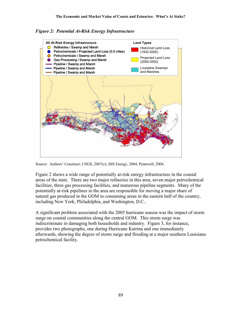
The Economic and Market Value of Coasts and Estuaries: What’s At Stake?
89
Figure 2: Potential At-Risk Energy Infrastructure
All At-Risk Energy Infrastructure
Refineries / Swamp and MarshRefineries / Swamp and Marsh
Petrochemicals / Projected Land Loss (0.5 miles)Petrochemicals / Projected Land Loss (0.5 miles)
Gas Processing / Swamp and MarshGas Processing / Swamp and Marsh
Pipeline / Swamp and MarshPipeline / Swamp and Marsh
Petrochemicals / Swamp and MarshPetrochemicals / Swamp and Marsh
Pipeline / Swamp and MarshPipeline / Swamp and Marsh
Pipeline / Swamp and MarshPipeline / Swamp and Marsh
Land Types
Historical Land Loss(1932-2000)
Projected Land Loss(2000-2050)
Louisiana Swampsand Marshes
Source: Authors’ Construct; USGS, 2007(c); IHS Energy, 2004; Pennwell, 2004.
Figure 2 shows a wide range of potentially at-risk energy infrastructure in the coastal areas of the state. There are two major refineries in this area, seven major petrochemical facilities, three gas processing facilities, and numerous pipeline segments. Many of the potentially at-risk pipelines in the area are responsible for moving a major share of natural gas produced in the GOM to consuming areas in the eastern half of the country, including New York, Philadelphia, and Washington, D.C.. A significant problem associated with the 2005 hurricane season was the impact of storm surge on coastal communities along the central GOM. This storm surge was indiscriminate in damaging both households and industry. Figure 3, for instance, provides two photographs, one during Hurricane Katrina and one immediately afterwards, showing the degree of storm surge and flooding at a major southern Louisiana petrochemical facility.

The Economic and Market Value of Coasts and Estuaries: What’s At Stake?
90
Figure 3: Storm Surge and Flooding Post-Katrina at Petrochemical Facility
Source: Photos courtesy of Air Products and Louisiana Chemical Association

The Economic and Market Value of Coasts and Estuaries: What’s At Stake?
91
Conjectures during and since the 2005 hurricane season have blamed coastal erosion for aggravated storm surge levels (Stokstad 2005).4 In other words, had some or all of the historic land loss not occurred, storm surge impacts would have been far less. Thus, increased storm surge exposure is another potential risk to energy infrastructure along the GOM. Figure 4 provides a map of storm surge along coastal Louisiana that occurred during 2005.
Figure 4: Storm Surge Areas, Hurricanes Katrina and Rita
Land Affected by Storm Surge
Katrina Storm Surge
Rita Storm Surge
Source: Authors’ Construct; FEMA 2007.
The next step in the analysis is to overlay the storm surge areas to all existing energy infrastructure to get a feel for additional potential exposure risk. The map provided in Figure 5 shows the infrastructure exposed to various degrees of storm surge and flooding during the 2005 hurricane season. If storm surge is in fact exaggerated by coastal erosion, then a considerable range of energy infrastructure assets would receive some economic benefit from mitigation and/or restoration. Figure 6 combines all of the prior analyses into an overview of all potential at-risk categories.
4 While anecdotally one could conclude that increased storm surge created by coastal erosion increased the damage suffered by many types of physical infrastructure, a comprehensive analysis has not been done to date.

The Economic and Market Value of Coasts and Estuaries: What’s At Stake?
92
Figure 5: Infrastructure in Hurricanes Katrina and Rita Inundation Zones
All Infrastructure in Hurricane Surge Areas
Petrochemical (Katrina)
Petrochemical (Rita)
Refinery (Katrina)
Gas Processing (Katrina)
Pipelines (Katrina)
Pipelines (Rita) Source: Authors’ Construct; USGS 2007(c); FEMA 2007; IHS Energy 2004; Pennwell 2004.
Figure 6: Potential At-Risk Infrastructure
All Infrastructure in Hurricane Surge Areas
Petrochemical (Katrina)
Petrochemical (Rita)
Refinery (Katrina)
Gas Processing (Katrina)
Pipelines (Katrina)
Pipelines (Rita) Source: Authors’ Construct; USGS 2007(c); FEMA 2007; IHS Energy 2004; Pennwell 2004.

The Economic and Market Value of Coasts and Estuaries: What’s At Stake?
93
The last step in the analysis is to examine other potential environmental impacts created by energy infrastructure, which in turn could be a function of coastal erosion and/or challenges associated with the operation of assets located in areas exposed to coastal erosion. Ruptures on existing pipelines in the coastal area were examined as a potential case in point. Figure 7 shows there were a large number of ruptures over the past decade that could have been caused, at least in part, by natural phenomena, “other,” or “unknown” reasons. While direct causality cannot and should not be assigned to coastal erosion, there is enough ambiguity in the nature of these ruptures that their relationship to coastal erosion merits further research. If in fact these ruptures were attributable to coastal erosion, the restoration and mitigation would provide additional environmental benefits, with economic value, that otherwise would go unrecognized.
Figure 7: Causes of Coastal Pipeline Ruptures, Historical and Projected Land Loss
Cause of Rupture
Criminal IntentEquipmentEquipment FailureNatural PhenomenonOperator ErrorOtherTransport AccidentUnknownAll At-Risk Land(Hist. & Proj. Losses/Swamp/Marsh)
Source: Author’s Construct; USGS 2007(c); LOSCO 2007.
The analysis presented in the prior figures shows a considerable range of assets that are potentially exposed to coastal erosion–created events. This approach should be the starting point in any valuation analysis of coastal restoration and energy infrastructure protection. The research, given its limited scope, did not move beyond the identification stage and so no conclusions can be drawn, other than that there is a considerable range of assets in the general coastal area that could be exposed to erosion-related problems. These assets are highly valued and critically important in the delivery of energy supplies to the entire country. Experiences after Hurricanes Katrina and Rita highlight this importance. Coastal restoration, therefore, appears to have the potential for some

The Economic and Market Value of Coasts and Estuaries: What’s At Stake?
94
significant collateral benefits in supporting these assets. No definitive conclusions about these benefits, or their order of magnitude, can be derived at this time without further investigation and research.
Conclusions Over the past several years, the relationship between energy production and infrastructure and coastal erosion has garnered significant attention, most of it negative and directed at pinning the blame for coastal erosion on energy industry activities. What is less recognized is that the energy sector has considerable assets along the coast, perhaps on the order of several billion if not hundreds of billions of dollars. It is in the best interest of these industries to protect these assets. The real challenge is identifying opportunities, through appropriate valuation techniques, of getting private and public coastal restoration activities aligned to maximize overall environmental benefits. The current regime would appear to suffer from a classic externalities problem that continues to go unaddressed. For instance, consider a situation where coastal erosion has forced a private firm to make a decision between investing in hardening a particular set of infrastructure investments or using coastal restoration to protect those assets. Further, assume that during the course of this valuation process, the physical hardening option is estimated to be slightly more affordable than the coastal restoration option. Clearly, a profit-maximizing firm will choose the least-cost option (holding other factors constant) and choose the physical hardening option over coastal restoration. However, if the additional public benefits were factored into this evaluation process, and the private firm could at least share in some of these potential benefits, an optimal economic solution to the problem could shift in favor of the coastal restoration option. The same valuation problem can occur in the public sector as well. Consider a public sector resource manager examining a variety of restoration projects that use habitat restoration, or some other natural resource–based measure, as the only criterion for project evaluation. This resource manager may choose one particular mitigation option over another that has higher overall economic value (due to energy infrastructure benefits) than the habitat-restoration approach only. If the resource manager were required to consider all benefits (including external economic benefits), it is likely that a different set of restoration choices may be developed.

The Economic and Market Value of Coasts and Estuaries: What’s At Stake?
95
References
Davidson, Jon P., Walter E. Reed, and Paul M. Davis, 1997. Exploring Earth: An
Introduction to Physical Geology. Upper Saddle River, NJ: Prentice Hall. Gonzalez, J.L., and T.E. Tornqvist. 2006. “Coastal Louisiana in crisis: subsidence or sea
level rise.” EOS. Vol. 87, No. 45, November 7, 2006. IHS Energy. 2004. Manufacturing and Industrial Plant Database. Louisiana Office of the Governor. Louisiana Oil Spill Coordinator’s Office (LOSCO).
2007. Environmental Baseline Inventory. Pennwell, Inc. 2004. Mapquest Database. Richardson, J.A. and L.C. Scott. 2004. The economic impacts of coastal erosion in
Louisiana on state, regional and national economies. Louisiana Department of Natural Resources. April 2004.
Stokstad, E. 2005. “Louisiana’s wetlands struggle for survival: New Focus.” Science.
Vol. 310, No. 5752, November 25, 2005. U.S. Department of Energy. Energy Information Administration (EIA). 2007a.
Petroleum Navigator. Internet website: http://www.eia.doe.gov/oil_gas/ petroleum/info_glance/petroleum.html
U.S. Department of Energy. Energy Information Administration (EIA). 2007b. Natural
Gas Navigator. Internet website: http://www.eia.doe.gov/oil_gas/ natural_gas/info_glance/natural_gas.html
U.S. Department of Energy (US DOE). 2007. The strategic petroleum reserve. Internet
website: http://pzl1.ed.ornl.gov/Sprpage.htm
U.S. Department of Homeland Security. Federal Energy Management Agency. 2007. FEMA Flood Recovery Database (Katrina, Rita).
U.S. Department of the Interior. Geological Survey. 2007a. A guide for teaching about
coastal wetlands. Glossary. Internet website: http://www.nwrc.usgs.gov/ fringe/glossary.html
U.S. Department of the Interior. Geological Survey. 2007b. Visual Glossary. Internet
website: http://www2.nature.nps.gov/geology/usgsnps/project/ home.html U.S. Department of the Interior. Geological Survey. 2007c. Coastal Louisiana’s
changing lands. Internet website: http://marine.usgs.gov/fact-sheets/ LAwetlands/lawetlands.html

The Economic and Market Value of Coasts and Estuaries: What’s At Stake?
96
U.S. Department of the Interior. Geological Survey. 2007d. Subsidence and fault
activation related to fluid energy production, Gulf Coast basin project. Internet website: http://coastal.er.usgs.gov/gc-subsidence/
U.S. Department of the Interior. Minerals Management Service (MMS). 2007. Mineral
Commodity & Revenue Statistics. Internet website: http://www.mrm.mms.gov/Stats/statsrm.htm

The Economic and Market Value of Coasts and Estuaries: What’s At Stake?
97
Chapter 6 – Economic Benefits of Coastal Restoration to the
Marine Transportation Sector
Di Jin Marine Policy Center Woods Hole Oceanographic Institution Woods Hole, MA 02543
Introduction The United States is the largest trading nation in the world (WTO 2005). Total merchandise trade was valued at $2.41 trillion1 in 2004 (Table 1). Ports are the primary gateway for international trade. Of all U.S. trade, ships carry close to 80 percent of the cargo by weight and close to 40 percent by value (Table 2). Each year, U.S. ports handle more than $800 billion in goods (Table 3). Marine transportation is an important sector in the national economy. A substantial literature examines (1) engineering and operational aspects of port development and management, (2) coastal ecology and environmental effects of air and water pollution (e.g., oil spills), and (3) erosion and coastal natural hazards. However, studies on the links between ports and the environment are sparse. We are unaware of any study on the benefits from coastal restoration to the marine transportation sector. In this chapter, we examine the potential benefits to shipping and ports from environmental improvements. Specifically, we identify direct and indirect links between environmental improvements and port operations and develop a framework for estimating the benefits from coastal restoration to the marine transportation sector. We will show that ports do benefit from improvements in the ecosystem. The remainder of the paper is organized as follows: section 2 presents an overview of the U.S. marine transportation sector; links between ports and the environment are discussed in section 3; a framework for estimating restoration benefits is described in section 4; and major findings of the study are summarized in section 5.
U.S. Marine Transportation Sector According to U.S. waterborne foreign trade statistics, compiled by the Department of Transportation, the total value of cargo handled by ports in the United States was $841 billion2 in 2003. As shown in Table 3, most of the cargo (33 percent, $278 billion)
1 In this chapter, all values are in 2005 dollars unless specified otherwise. Total trade value is the sum of exports and imports. 2 Excluding ports in Puerto Rico and the Virgin Islands.

The Economic and Market Value of Coasts and Estuaries: What’s At Stake?
98
passed through ports in California and Hawaii. Other dominant regions included the Northeast and the Gulf of Mexico regions, each handling 25 percent ($209 billion) and 19 percent ($157 billion), respectively. The top five states engaged in waterborne foreign trade were California, New York, Texas, Washington, and Louisiana (Table 4). Out of a total of 326 ports nationwide, 10 of them handle 85 percent of all containerized ship-borne cargo, with the ports of Los Angeles and Long Beach accounting for nearly 40 percent of all such cargo (U.S. Commission on Ocean Policy 2004). Table 5 presents a ranking of the top 30 ports in terms of cargo value. The ports of of Los Angeles, New York/New Jersey, and Long Beach each move over $100 billion of cargo annually. If we rank ports by cargo weight, two Gulf ports—South Louisiana and Houston—are on the top, each loading and unloading over 200 million short tons of cargo per year (Table 6). These ports play a dominant role in trade of agricultural products (e.g., grain), petroleum, and other industrial raw materials. International trade is carried by both U.S. and foreign-owned ships. The number and tonnage of U.S. merchant fleet by vessel types are shown in Table 7. In 2004, the U.S. merchant fleet consisted of over 1,000 vessels with a total over 45 million deadweight tons. Using IMPLAN software (MIG 2000) and U.S. national data, we calculated the water transportation sector’s output, employment, and related multipliers (Table 8). In 2003, the water transportation sector provided close to 60,000 jobs and generated $30 billion in gross revenues. The output value from the port and shipping sector was significantly higher than from other marine industry sectors such as commercial fishing and shipbuilding. The “Type II” multiplier for output for each industry sector measures the effect of changes in final demand (i.e., purchases by end users such as consumers or firms) for one industry on output in all other linked industries and on the income of people employed in those industries. For example, for each $1.00 of final demand for water transportation, $3.35 in industrial output and household income are generated in the United States. Employment multipliers are interpreted in much the same way. For example, each job in water transportation generates 11.14 jobs in the national economy. Note that the multiplier effect of the port and shipping sector is much larger than that of other marine industry sectors. The marine transportation sector has undergone substantial technological and organizational changes over the past three decades.3 Until the 1980s, ports had been considered to have natural hinterlands. All shipment points closer to a given port than to any other port comprised the natural hinterland of the port. Port proximity and inland cost are no longer the deciding factors in the international shipper’s port selection criteria. With ocean carriers and inland carriers jointly providing through-service and point-to-point rates, we now have shipping markets featuring intermodal competition. With intermodal competition, shippers are able to select carriers that provide services at the lowest logistics cost (e.g., inventory, warehousing, and transportation) rather than at the lowest transportation cost. Ports expand their activities to include influence or control
3 For studies on port productivity and efficiency changes, see de Neufville and Tsunokawa (1981), Bendall and Stent (1988), and Park and De (2004).

The Economic and Market Value of Coasts and Estuaries: What’s At Stake?
99
over the logistics network that lowers or minimizes a shipper’s logistics cost (Talley 1988). Environmental factors have become increasingly important in affecting port operation and, in turn, logistics costs (see Juda and Burroughs 2004).
Links between Ports and the Environment Ports are located in some of the most sensitive areas of the global ecosystem – estuaries and deep water lakes and rivers. Environmental effects associated with port operations include air emissions, water pollution, dredging, waste disposal, dust, and noise. There has been significant destruction of estuarine resources, wildlife, mangroves, and coral reefs worldwide in the vicinity of ports. Since the 1980s, environmental concerns have become an important factor in formulating port development and management decisions (Couper 1992). To ensure sustainable port development, ecological monitoring programs have been developed by many ports around the world to characterize environmental performance through appropriate monitoring and auditing. Typically, environmental auditing involves mapping of marine habitats, fishing areas, wetlands, zones of special scientific or cultural interest, recreational areas, and urban and industrial installations in a port region (Couper 1992; Wooldridge et al. 1999). In the United States, environmental mitigation has been used as a management tool capable of creating “win-win” situations for economic development interests and environmental resources managers. Ports that successfully integrate full consideration of environmental and resource impacts into the planning and construction of port development projects are likely to benefit from: (1) reduced permit delays and associated costs, (2) reduced uncertainty with respect to governmental approval of permits, and (3) increased public support for port development projects. In turn, environmental resource managers gain the cooperation of a significant set of developers and achieve “no net loss” of environmental resources4 (Wessel and Hershman 1988). In addition, an ecosystem-based management approach has been introduced to ensure the viability of port areas as natural resources as well as economic engines. The U.S. EPA’s Green Ports program is an example of an existing mechanism that incorporates environmental stewardship into port operation practices. The Green Ports program has been implemented by numerous U.S. ports along the Pacific, Gulf of Mexico, Atlantic, and Great Lakes coasts (U.S. Commission on Ocean Policy 2004). In theory, a framework for socially optimal management of an estuary may be designed to maximize the net social benefits from multiple uses by different sectors in the coastal economy (e.g., shipping and fishing). Marine transportation is one sector linked to the other economic and ecological sectors in many different ways. As in many other cases, the challenge is to strike a balance between benefits from port operations and costs associated with environmental degradation. In the existing literature, the environmental effects associated with port operations are considered an externality. In other words, port
4 For example, if wetlands are impaired or destroyed in one location, then equivalent wetlands must be created
or restored elsewhere (Polasky 2002).

The Economic and Market Value of Coasts and Estuaries: What’s At Stake?
100
operations are not affected by environmental quality. However, such treatment is incomplete, since the relationship between ports and the environmental is not unidirectional. Ports also benefit from improvements in environmental quality. There are multiple links between port operations and the ecosystem. We focus on how the ecosystem may affect port operations and how we might place a value on coastal restoration to the port and shipping sector. According to the U.S. Commission on Ocean Policy (2004), marine transportation may be significantly affected by changes in environmental and climate conditions, such as increased frequency or intensity of storms and changes in sea level. There are many historical examples of natural disasters (e.g., hurricanes, earthquakes, tsunamis, and droughts) affecting safe navigation and port operations. In 1994, the Houston Ship Channel was closed for several days when tropical rainfall caused flooding, dangerous currents, pipeline breaks and fires, and channel obstructions. In 2003, closures and limited operations occurred at major ports and shipping channels along the mid-Atlantic due to Hurricane Isabel. In 2005, the Port of New Orleans was closed for two weeks after Hurricane Katrina. Results from a study of the 1995 earthquake in Kobe, Japan, suggest that the Port of Kobe suffered major long-term traffic loss despite the restoration of damaged physical facilities. Pre-disaster mitigation or prevention action provides the best option for dealing with risks associated with natural disasters (Chang 2000). In fact, improving environmental and ecological conditions in a port region may be viewed as an important component of the port’s overall risk management strategy. For example, wetlands provide a variety of valuable ecosystem services, such as flood protection and erosion control (Farber et al. 2006). Wetland restoration also enhances a port’s capability to resist disasters. According to Adger et al. (2005), resilient social-ecological systems incorporate diverse mechanisms for living with and learning from change and unexpected shocks. Disaster management requires multilevel governance systems that can enhance the capacity to cope with uncertainty and surprise by mobilizing diverse sources of resilience. Here, resilience refers to the capacity of linked social-ecological systems to absorb recurrent disturbances such as hurricanes or floods so as to retain essential structures, processes, and feedback. Hazards in coastal areas often become disasters through the erosion of resilience, driven by environmental change and by human action. A study by Conner et al. (1989) has shown that along the northern Gulf of Mexico, hurricane impacts are often severe and long-lasting in wetlands that have been modified by human impacts. Dredging navigational channels for both port expansion (to accommodate larger ships) and regular maintenance is highly controversial due to the potentially negative effects on the marine environment (Juda and Burroughs 2004). Soil erosion leads to increased sedimentation in downstream waters and, in turn, to more dredging in harbors and shipping channels. Many studies indicate that grass and other vegetation cover are highly effective for soil conservation (Fullen 1998; Mazda et al. 2002). Furthermore, studies on dredging (Sohngen and Rausch 2001; Peng et al. 2006) have established the link between erosion control in watersheds and dredging sediments in downstream harbors. These

The Economic and Market Value of Coasts and Estuaries: What’s At Stake?
101
studies have shown that improved ecosystem management leads to a reduction in port dredging costs.
A Framework for Estimating Restoration Benefits From discussions in the previous section, we outline a framework for estimating benefits from coastal restoration to the marine transportation sector. As shown in Figure 1, the total benefits of restoration consist of both direct and indirect benefits. Direct benefits from restoration projects include increased resilience against natural disaster events, as well as improvements in soil conservation and associated reduction in dredging. Indirect benefits from restoration efforts reflect the improvements in overall economic-ecological conditions of the port region and increased public support for sustainable port development. These beneficial effects translate into reductions in the total cost of port operations and, in turn, the overall cost of ocean shipping. Marlow (1976) and Shneerson (1977) have discussed the theoretical measurement of economic benefits from shipping services to a national economy. Any inefficiency in marine transport affects the prices of final products (Wood 1975). An increase in transportation cost causes welfare losses in both importing and exporting countries.5 The empirical calculation of benefits from marine transportation is complex and requires considerable amounts of data on consumption, production, and trade of different goods in related countries. Costs associated with port operations constitute a portion of the total transportation cost. Damages to port facilities from natural disasters lead to higher port costs and in turn higher shipping costs. Thus, a precise measure of restoration benefits ought to consider broad effects throughout the economy. The specific methods we present in this chapter are partial analyses designed to highlight key links and develop preliminary valuation estimates with readily available data. In this section, we focus on the two direct benefits of restoration to ports as depicted in Figure 1. First, we quantify benefits from increased disaster resistance as follows: Suppose a wetland restoration project improves the effectiveness of disaster resistance of a port-ecological system. Combining information on disaster event probability, we can calculate the expected damage reductions (i.e., avoided costs), which are the benefits associated with the restoration project (Figure 2). As noted, ports may be closed after hurricanes. Wetlands provide a variety of valuable ecosystem services, such as natural flood control and shoreline stabilization. In this case, the effectiveness of disaster resistance may be measured as the reduction in the number of days of port closure. The expected benefit (B) is:
cpdB ⋅⋅∆=
where ∆d is the reduction in the number of port closure days, p is the event probability, and c is the daily cost of port closure. The costs of port closure resulting from natural disasters may be substantial. From the annual data on cargo values in Table 5, we can
5 The change in transportation cost affects producers and consumers in both trading nations. Associated welfare changes may be measured by changes in consumer and producer surpluses in both markets (Shneerson 1977).

The Economic and Market Value of Coasts and Estuaries: What’s At Stake?
102
calculate the average daily value for each port.6 For example, on average, the Port of Los Angeles handles $354 million in cargo per day and the daily value for the Port of New Orleans is $56 million. A restored estuary, or more healthy estuarine ecosystem, could potentially reduce the impacts on ports of natural disasters and could shorten length of port closure caused by coastal flooding, storm surge, or heavy rain events. If the port closure that could be expected from such an event were shortened by one day, avoided damage may be sizable.7 In addition to costs associated with delayed transport of cargo, natural disasters may also cause significant damages to port facilities. Damage to infrastructure for Louisiana’s public ports by Hurricane Katrina was estimated at $1.7 billion (Table 9). Similarly, we may quantify restoration benefits in terms of avoided costs of maintenance dredging. This idea is illustrated in Figure 3. For a wetland restoration project, one can first estimate the reduction in soil erosion resulting from increased vegetation coverage. Next, reductions in the volume of sediments to be dredged are quantified. Finally, avoided dredging costs are calculated as a measure of restoration benefits. An excellent illustration of the above approach is the case study by Sohngen and Rausch (2001) on dredging Toledo Harbor, Ohio. Annual quantity of sediments dredged in the port area was 850,000 cubic yards, costing $2.2 million.8 Some of the sediments were toxic, and special facilities were used for the disposal of contaminated sediments. The disposal cost was $4.1 million per year. The case study examined the economic benefits associated with a sediment reduction program for the upstream watershed (i.e., Maumee River basin). The sediment reduction program would lead to a 15% reduction in sedimentation rate and, in turn, a 15% reduction in dredging cost. The reduction in dredging volume in future years would result in an extended usage of existing disposal facilities and delayed construction of a new disposal facility for contaminated sediments. In addition, the new facility would be smaller and less costly than without the sediment reduction program. With the program, annual dredging and disposal costs would be $1.9 million and $3.1 million, respectively. Thus, the total benefit associated with the sediment reduction program was $1.3 million per year. If we extend Sohngen and Rausch’s study to the national level, the resulting benefits may be considerable.9 According to U.S. Army Corps of Engineers statistics for dredging cost in fiscal year 2005 (Table 10), at the national level, a total of 207 million cubic yards of sediments were dredged for harbor and channel maintenance at an average cost of $2.89 per cubic yard (USACE 2006b). The total cost for maintenance dredging was $598 million. Dredging as a result of Hurricane Katrina included an additional 1.3 million cubic yards at $4.29 per cubic yard (a total cost of $5.5 million).
6 Divide the annual value for each port by 365 days. 7 Actual calculation of port closure cost may be more complex, since not all cargo delayed is lost. 8 For the case study, we cite original values (in 1995 dollars) reported in Sohngen and Rausch (2001). 9 A detailed analysis of dredging costs should also consider beneficial use of dredged materials. For studies on beneficial use of dredged materials in different port areas, see Wagner (2000), Marcus (2000), and Yozzo et al. (2004).

The Economic and Market Value of Coasts and Estuaries: What’s At Stake?
103
Conclusions The United States is the world's largest trading nation. Ports are the primary gateway for international trade and handle more than $800 billion in goods annually. Marine transportation is an important sector in the national economy and provides over $30 billion in output value and 60,000 jobs. Marine and estuarine ports are located in the most sensitive areas of the marine ecosystem. While ports may impact these areas, they also derive benefits from the proper functioning of marine and estuarine ecosystems. We have shown that port operations are likely to be affected by a number of marine and estuarine ecosystem conditions. For example, natural disasters such as hurricanes may force ports to close. Also, environmental degradation may lead to an increase in soil erosion, causing elevated levels of sedimentation in harbors and channels, which impedes ship navigation. There are significant economic benefits of coastal restoration to the marine transportation sector. We have presented a framework for estimating these benefits. Specifically, the benefits may be calculated as avoided costs of natural disasters as well as avoided costs of dredging. An estimation of the total national benefit will need to be developed based on analyses of major ports around the country and a clear understanding of the incremental effects of individual restoration projects on erosion and flood control in relevant port areas.

The Economic and Market Value of Coasts and Estuaries: What’s At Stake?
104
References
Adger, W.N., T.P. Hughes, C. Folke, S.R. Carpenter and J. Rockstrom. 2005. Social-
ecological resilience to coastal disasters. Science 309:1036-1039. American Association of Port Authorities (AAPA). 2005. Damage estimates for
Louisiana’s public ports impacted by Hurricane Katrina. http://www.aapa-ports.org/ Katrina/DamageEstimate_louisianaports.pdf (Accessed September 25, 2006).
American Association of Port Authorities (AAPA). 2006. U.S. port rankings by cargo
value. http://www.aapa-ports.org/files/Statistics/2003_U.S._PORT_RANKINGS_ BY_CARGO_VALUE.xls (Accessed November 14, 2006).
Bendall, H.B. and A.F. Stent. 1988. Cargo handling productivity. Part 1. Maritime
Policy and Management 15(1):19-33. Chang, S.E. 2000. Disasters and transport systems: loss recovery and competition at the
Port of Kobe after the 1995 earthquake. Journal of Transport Geography 8:53-65. Conner, W.H., J.W. Day, R.H. Baumann and J.M. Randall. 1989. Influence of hurricanes
on coastal ecosystems along the north Gulf of Mexico. Wetland Ecology and Management 1(1):45-56.
Couper, A.D. 1992. Environmental port management. Maritime Policy and Management
19(2):165-170. de Neufville, R. and K. Tsunokawa. 1981. Productivity and returns to scale of container
ports. Maritime Policy and Management 8(2):121-129. Farber, S., R. Costanza. D.L. Childers, J. Erickson, K. Gross, M. Grove, C.S. Hopkinson,
J. Kahn, S. Pincetl, A. Troy, P. Warren and M. Wilson. 2006. Linking ecology and economics for ecosystem management. BioScience 56:121-133.
Fullen, M.A. 1998. Effects of grass ley set-aside on runoff, erosion and organic matter
levels in sandy soils in east Shropshire, UK. Soil and Tillage Research 46:41-49. Institute of Shipping Economics and Logistics (ISL). 2004. Shipping Statistics Yearbook
2004. Bremen, Germany. Juda, L. and R. Burroughs. 2004. Dredge navigational channels in a changing scientific
and regulatory environment. Journal of Maritime Law and Commerce 34(2):171-218.
Marcus, L. 2000. Restoring tidal wetlands at Sonoma Baylands, San Francisco,
California. Ecological Engineering 15:373-383.

The Economic and Market Value of Coasts and Estuaries: What’s At Stake?
105
Marlow, P.B. 1976. The indirect benefit of shipping to a national economy. Maritime Policy and Management 4:117-119.
Mazda, Y., M. Magi, H. Nanao, M. Kogo, T. Miyagi, N. Kanazawa and D. Kobashi.
2002. Coastal erosion due to long-term human impact on mangrove forests. Wetland Ecology and Management 10:1-9.
MIG, Inc. 2000. IMPLAN Professional version 2.0 (User's Guide, Analysis Guide, and
Data Guide). Stillwater, MN. Park, R-K. and P. De. 2004. An alternative approach to efficiency measurement of
seaports. Maritime Economics & Logistics 6:53-69. Peng, B., H. Hong, X. Xue and D. Jin. 2006. On the measurement of socioeconomic
benefits of integrated coastal management (ICM): application to Xiamen, China. Ocean and Coastal Management 49(3-4):93-109.
Polasky, S. 2002. The economics of wetland ecosystem restoration and mitigation:
discussion. American Journal of Agricultural Economics 84(5):1379-1380. Shneerson, D. 1977. On the measurement of benefits from shipping services. Maritime
Policy and Management 4:277-280. Sohngen, B. and J. Rausch. 2001. Case study of a market-based analysis: soil erosion in
the Maumee River basin. Pages 102-110 in A. Cangelosi, ed. Revealing the Economic Value of Protecting the Great Lakes. Northeast-Midwest Institute and National Oceanic and Atmospheric Administration, Washington, DC.
Song, D-W. and K-T. Yeo. 2004. A competitive analysis of Chinese container ports
using the analytic hierarchy process. Maritime Economics & Logistics 6:34-52. Talley, W.K. 1988. The role of U.S. ocean ports in promoting an efficient ocean
transportation system. Maritime Policy and Management 15(2):147-155. U.S. Army Corps of Engineers (USACE). 2006a. Tonnage for Selected U.S. Ports in
2004. Waterborne Commerce Statistics Center. http://www.iwr.usace.army.mil/ ndc/wcsc/portton04.htm (Accessed August 4, 2006).
U.S. Army Corps of Engineers (USACE). 2006b. FY 2005 Analysis of dredging costs.
http://www.iwr.usace.army.mil/ndc/dredge/dd05cos2.htm (Accessed September 25, 2006).
U.S. Commission on Ocean Policy. 2004. An Ocean Blueprint for the 21st Century. Final
Report. Washington, DC.

The Economic and Market Value of Coasts and Estuaries: What’s At Stake?
106
U.S. Department of Transportation (USDOT). 2003. U.S. International Trade and Freight Transportation Trends. BTS03-02. Bureau of Transportation Statistics. Washington, DC. http://www.bts.gov/publications/us_international_trade_and_ freight_transportation_trends/2003/excel/table_08.xls (Accessed September 5, 2006).
U.S. Department of Transportation (USDOT), Maritime Administration. 2006. U.S.
Waterborne Foreign Trade. http://www.marad.dot.gov/MARAD_statistics/EXP-2003.pdf and http://www.marad.dot.gov/MARAD_statistics/IMP-2003.pdf (Accessed November 14, 2006).
Wagner, R.J. 2000. Houston-Galveston navigation channel: blueprint for the beneficial
uses of dredge material. Coastal Management 28:337-352. Wessel, A.E. and M.J. Hershman. 1988. Mitigation: compensating the environment for
unavoidable harm. Pages 253-286 in M.J. Hershman ed. Urban Ports and Harbor Management. Taylor & Francis, New York.
Wood, J.N. 1975. Shipping and the UK economy. Maritime Studies and Management
3:71-79. Wooldridge, C.F., C. McMullen and V. Howe. 1999. Environmental management of
ports and harbors – implementation of policy through scientific monitoring. Marine Policy 23(4-5):413-425.
World Trade Organization (WTO). 2005. International Trade Statistics 2005. WTO
Publications, Geneva, Switzerland. http://www.wto.org/english/res_e/statis_e/ its2005_e/section1_e/i05.xls (Accessed August 29, 2006).
Yozzo, D.J., P. Wilber and R.J. Will. 2004. Beneficial use of dredged material for habitat
creation, enhancement, and restoration in New York-New Jersey Harbor. Journal of Environmental Management 73:39-52.

The Economic and Market Value of Coasts and Estuaries: What’s At Stake?
107
Table 1: Leading Exporters and Importers in World Merchandise Trade, 2004
Rank Exporters Value Share Importers Value Share
1 Germany 939.6 10.0 United States 1,571.3 16.1
2 United States 843.3 8.9 Germany 738.4 7.6
3 China 611.1 6.5 China 578.1 5.9
4 Japan 582.8 6.2 France 479.4 4.9
5 France 462.2 4.9 United Kingdom 477.4 4.9
6 Netherlands 368.9 3.9 Japan 468.2 4.8
7 Italy 359.6 3.8 Italy 361.6 3.7
8 United Kingdom 357.3 3.8 Netherlands 328.9 3.4
9 Canada 326.0 3.5 Belgium 294.0 3.0
10 Belgium 315.7 3.3 Canada 288.2 2.9
Units: Value in billions of 2005 dollars and share in percentage. Source: WTO (2005).
Table 2: U.S. International Merchandise Trade by Mode of Transportation, 2001
Mode of Transportation
Value
Share
Weight
Share
Water 38.4 77.7
Air 27.7 0.4
Truck 21.1 11.0
Rail 4.9 5.9
Pipeline 1.4 4.8
Other and Unknown 6.5 0.2
Total 100.0 100.0
Unit: Share in percentage. Source: USDOT (2003).

The Economic and Market Value of Coasts and Estuaries: What’s At Stake?
108
Table 3: U.S. Waterborne Foreign Trade by Region, 2003
Regions
Import
Value
Export
Value
Total Value
Total Value
Share
California and the Pacific Islands 232,203 45,512 277,715 33.0
Northeast Atlantic 160,266 49,139 209,405 24.9
Gulf of Mexico 103,816 53,464 157,280 18.7
Southeast Atlantic 48,973 24,140 73,113 8.7
Northwest Pacific 52,491 20,411 72,903 8.7
Florida 29,817 17,504 47,321 5.6
Great Lakes 1,697 1,977 3,675 0.4
Total 629,262 212,149 841,411 100.0
Units: Value in millions of 2005 dollars and share in percentage. Notes: The regions are defined as follows. Northeast Atlantic (ME, NH, MA, RI, CT, NY*, NJ, PA*, DE, MD, DC, and VA) Southeast Atlantic (NC, SC, and GA) Florida (FL) Gulf of Mexico (MS, AL, LA, and TX) California and the Pacific Islands (CA and HI) Northwest Pacific (OR, WA, and AK) Great Lakes (MN, MI, WI, IN, IL, OH, PA**, NY**) * Atlantic ports. ** Great Lakes ports. Source: Author’s calculation based on data from USDOT (2006).

The Economic and Market Value of Coasts and Estuaries: What’s At Stake?
109
Table 4: U.S. Waterborne Foreign Trade by State, 2003
State Import Value Export Value Total Value
California 230,279 45,342 275,621
New York 81,675 25,978 107,654
Texas 64,404 30,148 94,552
Washington 42,921 14,785 57,706
Louisiana 31,449 19,632 51,081
Florida 29,817 17,504 47,321
South Carolina 27,599 14,189 41,788
Virginia 22,686 13,670 36,355
Georgia 19,815 8,573 28,389
Maryland 21,487 6,028 27,514
Pennsylvania 14,690 1,491 16,181
Oregon 9,388 3,234 12,622
Puerto Rico 6,589 2,167 8,756
Mississippi 5,310 2,131 7,441
Massachusetts 5,469 766 6,236
Delaware 4,918 616 5,534
Virgin Islands 5,057 313 5,371
Alabama 2,653 1,553 4,206
New Jersey 3,416 182 3,598
Rhode Island 2,883 72 2,955
North Carolina 1,558 1,378 2,937
Alaska 183 2,392 2,575
Hawaii 1,924 170 2,094
Maine 1,255 296 1,551
Connecticut 1,298 79 1,377
Ohio 543 570 1,113
Michigan 400 471 871
Wisconsin 231 474 706
New Hampshire 608 76 685
Illinois 236 91 327
Minnesota 25 219 244
Indiana 143 31 174
District of Columbia 0 5 5
Total 640,909 214,630 855,539
Unit: Value in millions of 2005 dollars. Source: USDOT (2006).

The Economic and Market Value of Coasts and Estuaries: What’s At Stake?
110
Table 5: Major U.S. Ports by Value of Cargo, 2003
Rank Port Value
1 Los Angeles, CA 129,374
2 New York/New Jersey 107,247
3 Long Beach, CA 101,615
4 Houston, TX 52,887
5 Charleston, SC 41,737
6 Hampton Roads, VA 34,911
7 Tacoma, WA 27,912
8 Baltimore, MD 27,514
9 Oakland, CA 26,653
10 Seattle, WA 24,462
11 Savannah, GA 22,630
12 New Orleans, LA 20,576
13 Miami, FL 17,607
14 Portland , OR 12,518
15 Jacksonville, FL 11,909
16 Port Everglades, FL 11,129
17 Philadelphia, PA 10,934
18 Newport, RI 10,933
19 Morgan City, LA 10,715
20 Corpus Christi, TX 10,451
21 Beaumont, TX 10,193
22 South Louisiana 9,287
23 Kahului, HI 7,769
24 Texas City, TX 6,926
25 Boston, MA 6,022
26 Port Arthur, TX 5,886
27 Brunswick, GA 5,758
28 Hueneme, CA 5,683
29 Wilmington , DE 5,534
30 Lake Charles, LA 5,504
Unit: Value in millions of 2005 dollars. Source: AAPA (2006).

The Economic and Market Value of Coasts and Estuaries: What’s At Stake?
111
Table 6: Major U.S. Ports by Weight of Cargo, 2004
Rank Port Name Total Traffic
1 South Louisiana 224,187,322
2 Houston, TX 202,047,327
3 New York/New Jersey 152,377,503
4 Beaumont, TX 91,697,948
5 Long Beach, CA 80,066,130
6 Corpus Christi, TX 78,924,757
7 New Orleans, LA 78,085,209
8 Huntington - Tristate 77,307,514
9 Texas City, TX 68,282,902
10 Baton Rouge, LA 57,082,823
11 Mobile, AL 56,211,796
12 Lake Charles, LA 54,768,322
13 Plaquemines, LA 54,404,720
14 Los Angeles, CA 51,931,730
15 Tampa, FL 48,289,134
16 Baltimore, MD 47,399,120
17 Valdez, AK 46,758,499
18 Duluth-Superior, MN and WI 45,392,619
19 Pittsburgh, PA 41,034,808
20 Philadelphia, PA 35,219,613
21 Norfolk Harbor, VA 34,166,269
22 Pascagoula, MS 34,099,989
23 Freeport, TX 33,908,024
24 St. Louis, MO and IL 33,386,972
25 Paulsboro, NJ 30,485,654
26 Portland, OR 29,995,641
27 Portland, ME 29,709,345
28 Savannah, GA 28,176,658
29 Port Arthur, TX 27,570,039
30 Tacoma, WA 26,282,033
Unit: Total traffic in short tons. Source: USACE (2006a).

The Economic and Market Value of Coasts and Estuaries: What’s At Stake?
112
Table 7: U.S. Merchant Fleet, 2004
Tankers
Bulk
Carriers
Container
Ships General Cargo
Ships
Passenger
Ships
Total
Number 418 98 85 281 155 1,037
Tonnage 32,647 5,270 3,016 3,739 674 45,346
Unit: Tonnage is in thousands of deadweight tons (dwt). Note: Vessel statistics are based on country of domicile including ships of 1,000 gross tons and over. Source: ISL (2004).
Table 8: U.S. Marine Industry Sector Output and Employment, 2003
Industry Sectors NAIC
Codes
Output
Value
Type II
Multipliers
Employment Type II
Multipliers
Water Transportation 483* 31,959 3.35 58,491 11.14
Commercial Fishing 1141 3,658 3.00 97,127 1.58
Seafood Processing 3117 10,655 2.82 43,737 4.49
Ship Building 336611 15,889 3.35 89,847 3.96
Boat Building 336612 10,241 3.03 51,980 3.68
Unit: Output value in 2005 $U.S. millions. Note: NAIC 483 is the sector for ocean, costal, great lakes, and inland waters shipping Source: 2003 IMPLAN data (see MIG (2000) for IMPLAN software and data description).
Table 9: Hurricane Katrina Damage Estimates for Louisiana’s Public Ports
Port Damage Estimates
Port of New Orleans 1,600
Port of South Louisiana 2
Port of St. Bernard 40
Port Fourchon 61
Total 1,703
Unit: Damage in millions of 2005 dollars. Source: AAPA (2005).

The Economic and Market Value of Coasts and Estuaries: What’s At Stake?
113
Table 10: Dredging Costs for FY 2005
Types of Dredging Value Percent Volume Percent Unit Cost
Maintenance Dredging 597,604 62.5 206,547 81.0 2.89
New Work Dredging 327,604 34.3 41,845 16.4 7.83
Emergency Dredging 25,780 2.7 5,406 2.1 4.77
Dredging for Hurricane Katrina 5,503 0.6 1,282 0.5 4.29
Total 956,491 100.0 255,080 100.0 3.75
Units: Value in thousands of 2005 dollars, volume in thousand cubic yards, and unit cost in dollars per cubic yard. Source: USACE (2006b).
Figure 1: Benefits from Coastal Restoration to Marine Transportation
Coastal Restoration
Direct benefits Indirect benefits
Reduction inerosion
Increase inresilience
Long-term changesDisaster events
Improved regional economyand public support
Multiple uses
Total benefit

The Economic and Market Value of Coasts and Estuaries: What’s At Stake?
114
Figure 2: Benefit Estimation: Natural Disasters
Figure 3: Benefit Estimation: Maintenance Dredging
Wetlandrestoration
Reduction in erosion
Reduction in dredging
Avoided costs
Benefits
Effectiveness ofdisaster resistance
Wetlandrestoration
Disasterevent probability
Avoided costs
Benefits

The Economic and Market Value of Coasts and Estuaries: What’s At Stake?
115
Case Study: Soil Erosion in the Maumee River Basin and Dredging in Toledo
Harbor
Sohngen and Rausch (2001) described how to estimate the benefits of reduced dredging costs arising from lowering soil erosion upstream. In the Maumee River basin in northwestern Ohio, soil erosion from upstream land uses damages Toledo Harbor, into which the river drains. Annually, 850,000 cubic yards of sediment was dredged in the port area, costing $2.2 million. Some sediments were toxic, and special facilities were used for the disposal of contaminated sediments. The disposal cost was $4.1 million per year. The U.S. Army Corp of Engineers and the Natural Resource Conservation Service introduced conservation tillage across corn and soybean fields in the basin to reduce soil erosion. The program was expected to lead to a 15% reduction in sedimentation rate and, in turn, a 15% reduction in dredging costs. The reduction in dredging volume in future years would result in an extended usage of existing disposal facilities and delayed construction of a new disposal facility for contaminated sediments. In addition, the new facility would be smaller and less costly than without the sediment reduction program. With the program, annual dredging and disposal costs would be $1.9 million and $3.1 million, respectively. Thus, the total benefit associated with the sediment reduction program was $1.3 million per year (see Table 11).
Table 11: Annual Costs with and without Sediment Reduction
(millions of 1995 dollars)
Without Sediment
Reduction
With Sediment
Reduction
Dredging and transportation costs 2.2 1.9
Disposal Costs 4.1 3.1
Total Costs 6.3 5.0
Reference
Sohngen, B. and J. Rausch. 2001. Case study of a market-based analysis: soil erosion in the Maumee River basin. Pages 102-110 in A. Cangelosi, ed. Revealing the Economic Value of Protecting the Great Lakes. Northeast-Midwest Institute and National Oceanic and Atmospheric Administration, Washington, DC.
The Economic and Market Value of Coasts and Estuaries: What’s At Stake?
116
Chapter 7 – The Influence of Coastal Preservation and
Restoration on Coastal Real Estate Values
Judith T. Kildow, PhD Monterey Bay Aquarium Research Institute
One of the most clear-cut findings in the experimental literature on
environmental aesthetics is the consistent tendency for North
American and European groups to prefer natural scenes over built
views, especially when the latter lack vegetation or water features. Roger Ulrich (1983)
Introduction
After dredging out or filling in most of America’s estuaries for economic development over the past 50 years, there has been a policy shift to restore and save what is left of those fertile and unique coastal areas that scientists and engineers now tell us are some of our most valuable assets. Scientific evidence shows us that estuaries and wetlands are biologically productive areas, natural water filtration systems and buffers, and first line defenses against hurricanes and storm surges, protecting shoreline developments from costly damage. In addition, estuaries and oceans have purely aesthetic values. Knowing the value to society provided by estuaries is an important basis for justifying the costs involved in their restoration, since costs can run into the tens of millions of dollars for a single site, and especially since that restoration comes primarily from public funds. Who benefits from the restoration and how the benefits are distributed has important implications for public decisions. Estuaries are large and small, occupy urban as well as rural coastal settings, and many are in varying stages of deterioration. With such diversity, the costs of restoration can vary greatly. The beneficiaries can be large numbers of urban dwellers who benefit from urban redevelopments along restored harbor areas, or small numbers of fortunate coastal residents who have homes and businesses along the shore. Estuaries are inherently important to environmental and human health. Estuarine capacity to filter pollutants not only serves to provide a healthy environment for marine creatures to thrive, but it contributes to cleaner coastal waters for beach-going populations. This knowledge has produced new policy paradigms that encourage the restoration of polluted harbors as well as the reclaiming of coastal estuarine and watershed areas that were allowed to degrade in the past.

The Economic and Market Value of Coasts and Estuaries: What’s At Stake?
117
As estuaries, wetlands, and other natural coastal assets have become better understood, their functions have become more appreciated. Scholars have attempted to value estuaries, wetlands, and other natural assets along the coasts for decades. However, much of the research has concentrated on estimating substitute market values for estuarine functions that serve society, such as the value of filtration capacity, shore buffering, and fish nurseries. The focus shifts in this study to understand how the presence of healthy estuaries affects the market values of economic activities, e.g., real estate sales, recreation, and fishing—an approach that has not been well studied or documented before. Certain activities directly benefiting from restored estuaries have received the most attention from scholars: (1) fisheries that depend on estuarine spawning grounds and (2) recreation, as increasing numbers of people seek to enjoy the outdoors through birdwatching, kayaking and other types of boating, and nature hikes. These activities are covered in other chapters. Other sectors of the coastal marketplace, such as real estate values, have received far less attention from scholars. This paper focuses on the economic effect of proximity and access to coasts and oceans on real estate and property values. There is much evidence in the literature that property on or near the shore has considerably higher value than property away from the shore, indicating that buyers pay a premium for residences near beaches and with water views.
Water and Property For centuries, bodies of water have been population magnets. Environmental psychologists have attempted to explain this fascination. One prominent theory (Pitt 1989) explains the appeal of water to humans as the desire to return to the natural state of existence. Others have suggested that water and water views hold attention and interest more effectively than urban scenes (Ulrich 1981). The added value from waterfront properties not only has implications for added wealth for the buyers and sellers of these properties, but it has value to local communities and states through accompanying real estate taxes and property transfer taxes in many states, such as Florida and California. Property values have a large impact on our economy, although the exact magnitude of that impact has not been well documented. For purposes of this research, it is important to understand what affects coastal property values and the extent to which healthy coastal estuaries are important parts of the equation. What follows is a literature survey; some cases from the literature; a brief presentation of monetary estimates of the relationships between estuaries, other water bodies, and property values; an assessment of the limitations of the studies found and cited; and suggestions for further research needed to more accurately link estuarine restoration to property values.

The Economic and Market Value of Coasts and Estuaries: What’s At Stake?
118
A Survey of the Literature Determining the economic impact of estuarine restoration on property values is not a simple exercise. Searching the literature requires assumptions about which attributes of healthy estuaries increase people’s desire to live near or along them, and therefore, increase the demand for healthy estuaries. Some of the more obvious attributes are unpolluted waters, interesting wildlife to view, and ready access to recreational opportunities such as boating, kayaking, canoeing, etc. Economic evidence demonstrates that the aforementioned recreational activities have been increasing over the past decade, and contribute significantly to the U.S. economy (U.S. Department of the Interior and Department of Commerce (2000, 2005). One of the benefits of estuary restoration is improvement in water quality, which prompts the gradual return of the wildlife that once thrived there. Hence, one might conclude that healthy, restored estuaries that provide those amenities will be of interest to those who purchase coastal properties, and will have a positive influence on real estate values with proximity to them. When searching the literature for evidence of these links, I tested this assumption for both large and small estuaries, located in urban and rural locations. While many studies link air quality with property values (Poor et al. 2006)1 the literature search turned up only a few that link water quality with property (Leggett and Bockstael 2000). However, many studies estimated premium values2 for properties with ocean views and waterfront locations, which provided circumstantial evidence.
The literature survey revealed several categories of studies—those that provided links between estuaries and/or estuary/harbor restoration and property values, and studies linking other water bodies to property values. The three studies with direct links to estuaries/harbor environments used a combination of either hedonic pricing methods and/or contingent valuation/conjoint analysis surveys. These are:
1. A hedonic property study3 that compares housing prices in a well-defined, small area of homes along the Chesapeake Bay with varying degrees of water quality degradation (Leggett and Bockstael 2000);
2. A hedonic property model that estimates the marginal value of water quality in
the St Mary’s River Watershed of the Chesapeake Bay (Poor et al. 2007); and
1 From Chattopadhyay (1999); Palmquist and Israngkura (1999); and Zabel and Kiel (2000). 2 Premium value indicates the added value a property commands, based on its water-based amenities compared to a similar property without that amenity. 3 Hedonic Pricing Method assesses the value of an environmental characteristic by examining market transactions for similar goods with differing key features, to determine whether that feature contributes to the price of a specific good. In real estate markets this is most often the comparison of two homes of similar design and quality but located in different physical locations (e.g., waterfront versus non-waterfront).

The Economic and Market Value of Coasts and Estuaries: What’s At Stake?
119
3. A study that combined two methods, hedonic methods and conjoint analysis (Braden et al. 2004). This study used housing market data and also measured the preferences of homeowners in both Lake County, Illinois, and in Waukegan, the county seat where the harbor restoration was the focus for the study. 4
The other category includes studies linking water amenities to property values in a variety of ways. These were included as surrogates from which analogies could be drawn for estuaries. These studies include:
1. Comparison of property flood insurance rates based on proximity to flood plains reported as a surrogate for coastal properties buffered by estuaries.
2. Studies estimating premium value of waterfront location or water views.
Case Studies from the Literature
Studies Using Hedonic and Conjoint Choice Methods to Determine the Importance
of Water Quality to Property Prices
A. Leggett and Bockstael (2000) provide evidence that people are willing to pay more for better water quality. The authors use hedonic techniques to show that water quality has a significant effect on property values along the Chesapeake Bay. This study demonstrates the potential benefits from an illustrative water quality improvement. Their assumption was that pollution sources might be unwanted neighbors, something other studies had ignored. “This paper takes advantage of a unique geographical environment, a lively housing market along an estuary with large variations in water quality, to show that improvements in water quality can have a positive and significant effect on property values” (Leggett and Bockstael 2000, p. 127).
Controlling for multiple types of landscape variables—including population density, proximity to major cities, pollution emitters, and a host of other variables—the authors found that the variable for coastal properties with identifiable importance for buyers was proximity to water, “having a positive and significant effect on price”….. “After accounting for omitted variable bias and after correcting for spatial autocorrelation, we still can conclude, but now with considerably more confidence, that waterfront homeowners have a positive willingness to pay for reductions in fecal coliform bacteria concentrations” (Leggett and Bockstael 2000, p.142). There are two major considerations when using water quality as the independent variable linking property values with healthy estuaries or other aquatic bodies. One is “perceived” quality that you can see or smell, such as turbidity, cloudiness, and eutrofied systems. The other is “evidence-based” quality such as fecal-coliform degradation, which is mostly invisible and where crucial information is essential to demonstrate quality. Presumably, both considerations of water quality information affect personal choice for buying properties. With water found to be
4 Conjoint Choice Analysis uses the ranking of potential characteristics (to include environmental attributes) by respondents to approximate the value of alternative goods, services, or assets.

The Economic and Market Value of Coasts and Estuaries: What’s At Stake?
120
the most important consideration in assessing property value, the health effects of clean water were believed by the authors to be important considerations for buyers, and thus fecal coliform count linked to the property values was believed to be a strong indicator. To estimate their model, the authors used a strip of shoreline with definable divisions in Anne Arundel County, Maryland, on the western shore of the Chesapeake Bay, with reliable water quality monitoring. The data were drawn from 1,183 sales transactions of waterfront properties occurring only along navigable sections of tributaries to the main stem of the Chesapeake Bay, between July 1993 and August 1997.5 The independent variable data included attributes of the homes and also the results of fecal coliform counts, monitored from Memorial Day to Labor Day, at 104 stations along the shoreline of the Bay.6 The authors found that of the 6,704 residential waterfront properties in Anne Arundel County, 494 had fecal coliform bacteria concentration values exceeding the EPA standard of 200 counts per 100 ml. The hypothetical improvement is one that would reduce fecal coliform counts at all waterfront properties to the state standard (EPA standard) of 200 counts per 100 mL (Leggett and Bockstael 2000, p. 142). Improving water quality to the EPA/state standards for all 494 homes on or near waters that did not meet EPA standards, the authors estimate would have potential economic benefits of $12.15 million with a 95% confidence interval of $3.789 million to $20.501 million (Leggett and Bockstael 2000, p. 142). They also indicated their results were conservative because they did not reflect all of the benefits of water quality improvements to factors such as “benefits to owners of waterfront properties along tributaries without monitoring stations—about 750 parcels; they ignored potential benefits to near-shore property owners,” etc. (Leggett and Bockstael 2000, p. 142).
B. St. Mary’s River Watershed
The Poor et al. (2007) study of the St. Mary’s River watershed is the second study where authors estimated the value of clean water bodies as revealed by home prices of nearby residences. The research focused on the St. Mary’s River watershed, a sub-watershed of the Chesapeake Bay on the western shore. This study provides estimates of marginal values of ecosystem indicators—total suspended solids and dissolved inorganic nitrogen—that can be directly linked to property values. The study area examines a peninsula surrounded by the Potomac and Patuxent rivers in a small county in southern Maryland where, according to the authors, citizens had complained about recent declines in water quality of the river. The uniqueness of this study is the use of both waterfront and non-waterfront properties for a hedonic property valuation to estimate the marginal prices of ambient water quality. The assumptions were that non-point run-off was responsible for much of the water quality decline and that much of that was the result of changing land uses. The purpose of this study was to demonstrate the “willingness to pay” of local homeowners to allow the river to return to health through the lens of house sale prices. The authors used total suspended solids and dissolved inorganic nitrogen as the water quality variables that were carefully monitored at 22 stations throughout the
5 The sales information came from the Maryland Tax Assessment database. 6 Collected and analyzed by the Anne Arundel County Department of Health.
The Economic and Market Value of Coasts and Estuaries: What’s At Stake?
121
watershed. They used a hedonic price model for 1,377 residential property sales occurring within the St. Mary’s River watershed over a period of four years between June 1, 1999, and May 31, 2003. Using real estate data from several sources and prices converted to January 2003 constant dollars, the authors used geo-coded data to locate each property used in the study. Both waterfront properties (which make up 2% of the properties considered) and all other properties reveal statistically significant relationships between water quality measures and home price. Without going into the complexities of their work, their results indicated that a one unit (mg/L) increase in total suspended solids had a negative impact on the average housing price (204,823) within the watershed of $1,086. A 1-unit (mg/L) increase in dissolved inorganic nitrogen, a contributor to eutrophication, had a negative impact on the average housing price ($200,936) in the watershed of $17,642 (Poor et al. 2007). The ranges for the average water quality indicators across the monitoring stations with the sample are 8.918 mg/L to 12.851 mg/L for total suspended solids and .082 mg/L to .956 mg/L for dissolved inorganic nitrogen. Taken across all homes in the study region, these marginal values clearly account for millions of dollars that could be gained from water quality improvement.
C. Waukegan Harbor
People often forget that many commercial harbors lie within estuaries. Surveying the regeneration of urban harbor areas around the United States, one finds that harbor clean-up often goes hand in hand with new commercial and residential developments that ultimately raise the property values of formerly undesirable and rundown areas. A recent study (Braden et al. 2004) of Waukegan Harbor in Lake County, Illinois—a Superfund site—reflects the local and regional population’s attitudes about restoring their harbor; i.e., that positive things would happen if it were cleaned up. The study also uses a hedonic pricing technique with actual housing data to complement the attitude survey. While Waukegan Harbor is not an estuary, the benefits derived from restoration and clean-up in Waukegan Harbor are likely to be similar to those for similar harbors in estuaries. Waukegan Harbor was designated one of the Great Lakes Areas of Concern (AOC) in the 1980s by the International Joint Commission (IJC) with serious contamination. EPA placed two sites within Waukegan Harbor on the National Priority List (NPL) under Superfund legislation in 1980 (U.S. EPA 1980) because of PCB contamination from industrial discharges between 1948 and 1971. The AOC designation indicated impairments to five beneficial uses: beach closures, degradation of phytoplankton and zooplankton populations, degradation of benthos, restrictions on dredging operations, and loss of fish and wildlife habitat. As a result, the surrounding communities and the state have been affected by major tax losses, according to economic data that has been generated over the past decade. Clean-up of the harbor began in the early 1990s, which led to “noteworthy improvements in the harbor’s environmental condition” (Braden et al. 2004). However, additional remedial action, estimated at $21 million, is still required to de-list the site Not only would this last step in the clean-up process eliminate the remaining “beneficial use impairments,” with their accompanying economic impacts, but it would relieve the

The Economic and Market Value of Coasts and Estuaries: What’s At Stake?
122
community of its “stigma of contamination” and probably increase the desire for development and rejuvenation of the harbor area, which would have ripple effects throughout the area (Braden et al. 2004, p. 488). Without any calculations and research, one could surmise that the cost of the final clean-up, an estimated $21 million, would probably be more than recovered economically by the positive effects it would have on the community, or so the results of this study would indicate. “Overall, this study suggests that cleanup of the Waukegan Harbor AOC, including but not limited to sediment remediation, is likely to increase the value of residential properties in the City of Waukegan by an amount denominated in the hundreds of millions of dollars, and perhaps by significant amounts elsewhere in the region as well” (Braden et al, 2004, p. 488). This study used both hedonic pricing methods and conjoint choice surveys, which revealed multiple dimensions of how residents chose housing. The authors describe four aspects of this study, which make it unique. First, they considered property values not just in the immediate vicinity of the harbor, but throughout the county. Here they tested the effect of a stigma, a Superfund site, to determine the geographic effect of this reputation. Second, this study combines survey and market data. They combined the flexibility of the survey approach and the real behavior and financial commitments of real property data. Third, instead of using an open-ended contingent valuation survey design, they adopted a conjoint choice format where individuals select between alternative versions of a particular good. Fourth, the survey component opened the door to determining future developments as well as apparent effects of past and present conditions. This allowed them to estimate potential effects of the clean-up of the harbor on property values, both from a market value and human attitude perspective. The authors (Braden et al. 2004) chose one group to query for their study, the homeowners. “They are the dominant voting population of most communities and are important in the formation of local public policies (Braden et al. 2004).” The thinking was that if homeowners’ interests were perceived to be well served by the clean-up in raising their property values, they might be more willing to support public investment in the restoration of their harbor. As taxpayers in the community, they are important stakeholders to help finance the clean-up through local tax collections (Braden et al. 2004). The results of the study indicated that the clean-up of the harbor was perceived to be more valuable to those living in the city of Waukegan than to those living throughout the rest of the county. The authors found that the presence of other amenities such as parks, nature, etc. were of less importance than the actual clean-up of the harbor. For homeowners in the city of Waukegan, the authors estimated a willingness to pay for harbor clean-up of $400 million, or approximately 16 to 19 percent of all Waukegan property values. The reported “willingness to pay” throughout the rest of Lake County, where Waukegan is the county seat, amounted to approximately $7 to $12 billion, or between 15 percent and 26 percent of home values elsewhere in the county (Braden et al. 2004). As is often the case, the willingness to pay increased with income—apart from the effects of income, Waukegan households, on average, would pay approximately 27
The Economic and Market Value of Coasts and Estuaries: What’s At Stake?
123
percent more for full clean-up than non-Waukegan homeowners. This study reports that, of the other studies done for Great Lakes sites in the past, the average was about 15 percent of existing property values within a radius of 5 to 6 miles (Braden et al. 2004). The authors find that the results for Waukegan Harbor were higher than those found by studies of three other Great Lakes areas (Calumet, Indiana; Hamilton, Ontario; and Ashtabula County, Ohio). According to the authors, Waukegan Harbor is unique, with a powerful community sense of stigma throughout the region from their proximity to a Superfund site. The implications of the Waukegan experience can be seen in estuaries. While careful research on property values has not been undertaken to value the impact of restoration in California’s Oakland Estuary, the initial results of that restoration speak for themselves: by unanimous vote (Heredia 2006), the city approved development plans for 31,000 housing units near the estuary, 200,000 square feet of retail units, a 170-slip marina, parks, and promenades, with additional restored wetlands being constructed on Oakland’s shoreline and scheduled for completion by 2010.
Studies Linking Other Water Bodies and Amenities to Property Values
A. Linking Risk and Insurance Rates to Property Values
Estuaries often are cited as natural buffers that help prevent property loss along the shore in the face of strong storms. In other words, properties buffered by estuaries are probably at less risk for damage than those located directly along beaches and non-protected shorelines. If insurance rates correctly assess risk to property in flood zones, they should convey a savings in property insurance premiums for coastal homes that enjoy the benefit of estuarine buffers versus non-buffered coastal areas. Insurers are interested primarily in assessing the risk of a particular piece of coastal property from storm surges, hurricanes, and even tsunamis in selected areas, which can cause flooding at the very least, and undermine or even destroy properties at the most serious level. Estuaries and wetlands are well understood to be buffers and flood protectors for homes and commercial buildings and other physical infrastructure, so their value as the first line of defense for physical properties near the coast should be high. Knogge et al. (2004) estimate the value of indirect functional benefits of coastal wetlands for protection from coastal impacts of climate change to be between $3 million and $13 million/km. It is difficult to know how the insurance industry estimates these values, because the formulae they use for their actuarial equations are proprietary. In a study by Bin et al. (2006), the authors find that location within a flood zone lowers the property value. The authors employed hedonic property price method to examine the effects of flood hazards on coastal property values in mainland Carteret County located along the Atlantic coast of eastern North Carolina. With the highest point in the entire county at 51 feet above sea level, most of the county is low-lying and prone to flooding. The authors controlled for most of the amenities that would influence the price of coastal properties, because without such controls floodplain location appears to have no effect on housing values.

The Economic and Market Value of Coasts and Estuaries: What’s At Stake?
124
Their results showed that “flood insurance premiums convey risk information to potential buyers in the coastal housing market.” Results suggest that location within a floodplain lowers the average property’s value by 7.3 percent or $11,598. Furthermore, they found that the price discount for location within a higher risk area for flooding is significantly larger than the price discount for location within a lower risk area. Location within a 100-year floodplain lowers the average property’s value by 7.8 percent, or $12,325, while location within a 500-year floodplain lowers average property value by 6.2 percent, or $9,849. They calculated the flood insurance premiums for the various flood zones and found that the capitalized values of the insurance premiums are comparable with the sales price differentials. This study utilized a total of 3,106 residential property sales records from September 2000 to September 2004. Sales prices were inflation-adjusted using the Consumer Price Index to report figures in September 2004 dollars. The average home sales price in the data set was $163,911. The homes were on average 24 years old with 1,633 total square feet. Approximately 16 percent of the properties were classified as new (sold within a year from the date built).
B. Estimated Premium Value of Waterfront Location or Water Views for a Range of
Salt and Fresh Water Bodies (surrogates, assuming that estuaries are waterfront or
nearly so)
This category shifts the emphasis of the previous cases from the added property value derived from estuarine restoration to the value added to a property merely by being near water. This category does not help us determine the value of restoring an estuary or what people would be willing to pay for restoration. However, it demonstrates the importance of water (and implicit water quality) to property values, and gives us another piece of evidence concerning values. If one looks beyond the estuary to water bodies in general, studies consistently demonstrate that the price of a property with a view or location on water is much higher than those without those same amenities. What follows are thumbnail sketches of studies that provide examples of value added to properties from water-based amenities. The following variables were used in these studies, providing a framework for estimating premium values. Variables included:
•••• Proximity to water.
•••• Quality of view.
•••• Price of housing and neighborhood.
•••• Location: urban, suburban, or rural.
•••• Availability: Communities with limited numbers of homes with water views command higher premiums than those communities with a higher percentage of homes with water views.
•••• Using sales transactions as the base or tax assessments or both.
•••• Residential real estate cycle and how premiums are affected.
•••• Water quality elements of potential influence (Connor 2005).
•••• Proximity to water recreational opportunities.

The Economic and Market Value of Coasts and Estuaries: What’s At Stake?
125
1. A recent study by Nelson et al. (2005) surveyed available literature (1973–2002) on the influence of natural amenities as residential externalities affecting property ownership and values. None of the studies examined addressed estuaries or wetlands, but many studies addressed such amenities as lakes, oceans, and parks. Each study indicates a positive impact for water, ranging from a 90 percent increase in value for direct frontage for a single-family home on Lake Erie, to a 4–11 percent premium for a condominium with a lake view. This study reports on a broad range of premium values based on many of the variables mentioned above, describes different methods of measurement, and assesses effectiveness of the methods for applications.
2. Bourassa, Hoesli, and Sun (2004) did a study of Auckland, Christchurch, and
Wellington, New Zealand, residential sales for 1986 to 1996 and found that: (1) implicit prices of aesthetic externalities move with the real estate cycle, and (2) the percentage premiums for water views are greatest in Christchurch, which has the smallest percentage of properties with water views, and lowest in Wellington, which has the highest percentage of properties with views.
3. Pompe and Rhinehart (1995) found that the quality of two beaches in South Carolina
were a major influence on real estate values. Through the use of hedonic pricing methods, the authors estimated the values of wider beaches to vacant lot and single-family homes with or without water frontage; they also looked at factors that diminish the beach experience.
4. Seiler et al. (2001) examined the influence of Lake Erie views on property values.
Half of the samples of homes in this study have a clear water view while the other half, which consist of adjacent properties, do not. Lake Erie often provides an ocean-like view because of its size, and it generates waves large enough to surf. The study results show that having a lake view increases home value on average by $115,000, or by approximately 56 percent.
5. In a rural area in the United Kingdom around the Forest of Dean in Gloucestershire,
Garrod and Willis (1992) examined the property value effect of different types of natural open space. The nearby presence of a canal increased the value of the average house by 4.9 percent, while the proximity of at least 20 percent woodland cover raised it by 7.1 percent. Open water did not have an observable effect, and the presence of marshland reduced housing prices (Polis Project 2001).
6. Coastal preservation also has been shown to have an impact on property values, even
though development potential is often constrained along coastlines to protect significant natural features. The California Coastal Commission, established in 1972 to protect the California coast, is one such vehicle to serve that purpose. Frech and Lafferty (1984) estimated that the Commission’s work raised the value of local housing in two ways: by preserving a positive externality (the coastline) that would otherwise be destroyed, and by reducing the amount of land available for housing. They found that in the zone closest to the coast, housing prices were 7.6 to 13.4 percent higher ($2,882 to $5,040) than comparable homes more than 0.5 miles inland.

The Economic and Market Value of Coasts and Estuaries: What’s At Stake?
126
In a separate study, Kniesel (1979) found a 7 to 21 percent increase in housing prices for properties 4.5 miles from the coast.
7. In Maryland, the Critical Areas Commission limited residential development on land
abutting the Chesapeake Bay in 1986. Prices of housing with water frontage in the critical area increased by 46 to 62 percent (Parsons 1992). Housing prices in the critical area without water frontage increased from 14 to 27 percent. Even as far as 3 miles from the critical area, there was a 4 to 11 percent price increase (Polis Project 2001).
8. Several studies (Major and Lusht 2004; Benson, Hansen and Schwartz 2000; Polis
Project 2001) analyzed the placement of buffers between the ocean and homes, indicating significant drops in price due to the distance, or apparent distance, from the ocean. Most studies of this type focus either on the quality of a view of the water or the proximity to the water (which can alter the quality of the view). In the former, a view can enhance the value of a home anywhere from 8 percent (e.g., in Fairfax County, Virginia) to 126 percent (e.g., in Bellingham, Washington), according to one method of analysis using county tax records (Rodriguez and Sirmans 1994).
9. Major and Lusht (2004) found that proximity to the ocean has a different value from
proximity to a bay in their study of Stone Harbor and Avalon sites in New Jersey. They used distance to water as the key variable assuming that convenience and views would be the same since both are contiguous beach communities, one facing a bay and the other facing the ocean. The authors also drew property values from sales transactions. In this study, beachfront proximity had a premium value of 207 percent compared to a property two blocks away. A bayfront location added 73.2 percent.
10. Inland waterways also contribute to home values. Canals and waterways have been
built into developments to give houses frontage on a body of water to boost the price. Some of these have the additional attributes of wildlife and/or availability of boating (Nelson et al. 2005). The price premium found in this study was approximately $175 per frontage foot to sale price in the sample. While significant for the local market, it is relatively modest compared with the 142+ percent premiums for oceanfront and even lake proximity. This would make sense, however, in view of the more spectacular views and probably greater recreational opportunities available for these latter sites.
11. Epp and Al-Ani (1979) found that water quality of streams had an effect on home
prices. This study found that pH levels low enough to limit recreational use affected housing prices. Acidity from minerals and CO2 prevented recreation, and therefore, limited prices.
Table 1: Summary of the literature findings7
7 Feel free to contact the author at National Ocean Economics Program for more information.

The Economic and Market Value of Coasts and Estuaries: What’s At Stake?
127
Study Water Body Variables
Considered
Base Price Value Added8
Bin et al. (2006)
Atlantic Ocean NC (Carteret county)
Flood zone Median price <7.3%> or <$11,598>
Bourassa, Hoesli and Sun (2004)
New Zealand Water views Median price % value is increased; greatest increase where supply of properties is low
Braden et al. (2004)
Lake Michigan (Waukegan Harbor)
Restoration and Clean-up harbor (Superfund site)
Median price Willingness to pay 16-19% of property values
Epp and Al-Ani (1979)
Pennsylvania Water quality of streams
Mean price pH levels affected housing prices
Frech and Lafferty (1984)
California Coastal preservation Median price 0-0.5 miles inland: 7.6%-13.4% or $2,882-$5,040
Garrod and Willis (1992)
UK: Gloucestershire
Natural open space Median price Canal: 4.9% Woodland cover: 7.1% Open water: 0% Marshland: negative
Kniesel (1979) California Coastal preservation Median price 0-4.5 miles inland: 7.%-21%
Knogge et al. (2004)
Estuaries Protection from coastal impacts of climate change
Median price $3M-$13M/km
Leggett and Bockstael (2000)
Chesapeake Bay (Western Shore)
Water quality improvement
Median price $12.15 million on 494 homes
Major and Luscht (2004)
New Jersey Proximity to ocean vs. bay
Values from sales transactions
Beachfront 207% higher than two blocks from ocean Bayfront 73.2% higher than two blocks from bay
Nelson et al. (2005) Literature survey
Lake Erie Proximity to water Median price Ranges from 90% direct frontage (single family) to 4%-11% lake view (condo)
Nelson et al. (2005)
Arlington, TX Inland waterways and canals
Premium on sales price
$175 per frontage ft.
Parsons (1992) Chesapeake Bay Proximity to water Median price With water frontage: 46-62% Without water frontage: 14-27%
Polis Project (2001)
Chesapeake Bay Proximity to water Median price 3 miles away: 4-11%
Pompe and Rhinehart (1995)
South Carolina Quality of beaches Real estate values
Not specific
Poor et al. (2007)
St. Mary’s River (Chesapeake Bay)
Water quality: total suspended solids; Water Quality: dissolved inorganic
Median price TSS: <$1,086> N: <$17,642>
8 These values are in nominal dollars.

The Economic and Market Value of Coasts and Estuaries: What’s At Stake?
128
Study Water Body Variables
Considered
Base Price Value Added8
nitrogen
Rodriguez and Sirmans (1994)
VA and WA Proximity to water Tax Records VA: 8% WA: 126%
Seiler et al. (2001)
Lake Erie View Median price 56 % or $115,000
Suggestions for Further Research There is a lack of research to link estuarine restoration with property values, since only three studies were found that could be considered of direct interest. This field is ripe for study from multiple perspectives. Organized studies need to be conducted that track the value of properties that border or view estuaries and other relevant natural assets. Estuaries share the attributes of many of the water bodies examined in the studies reviewed here. Therefore, we would expect proximity to estuaries and improvement in estuarine environmental quality to have significant impacts on home values. Additionally, estuaries differ from these bodies in the type, abundance, and diversity of wildlife and plants that live near estuaries. Because estuaries are tidally influenced, the effects of tidal change—especially the presence of tidal flats at low tide—may have effects on estuarine home prices not considered in the studies above. Estuaries may also influence local home values through their capacity to (1) filter pollutants from run-off and the avoided costs of a filtration plant, (2) buffer built assets from storm damages and the avoided costs of armoring the shore, and (3) provide nursery spawning grounds for fish and wildlife of recreational and commercial interest. However, no published study of a particular site can link these indirect estimates to either individual or community-wide property values. For example, despite growing recognition of the importance of estuaries as buffers that limit property damage from predicted intensity and frequency of hurricanes and major storms, no published studies reflect how much value estuaries could add to coastal properties through lower insurance rates and avoided costs of damage. Only one study (Knogge et al. 2004) addresses the value of coastal wetlands in protecting shorelines from the impacts of sea-level rise. Insurers are interested in sea-level rise and climate change responses as they affect coastal properties.9 There is a growing body of literature about this aspect of valuation, but more from the point of view of how rising sea levels will affect physical assets specifically or how they will affect and change the natural assets of estuaries and wetlands, rather than how those effects will influence real estate prices (Knogge et al. 2004).
9 Presentation of C. Hedde at Disaster Round Table. National Academies, Washington DC, March 27, 2007.

The Economic and Market Value of Coasts and Estuaries: What’s At Stake?
129
In addition, coastal wetlands and estuaries are proven community assets as pollutant filters (Knogge et al. 2004). As development replaces nature’s absorbent capacities with hard surfaces, estuaries become increasingly important in providing communities with clean water. The exact value to individual properties or community-wide is unknown. With increasing interest in wildlife viewing and birdwatching, healthy estuaries provide a strong economic base as a destination for tourists and local populations to enjoy the outdoors. Their economic value through direct price impact to properties in proximity to estuaries, or even via tax revenues to entire communities that feature estuaries, have not been assessed.
Harbors are another area much overlooked. Waukegan Harbor (Braden et al. 2004) is the only study of note that provides carefully compiled evidence of the attitudes of the property owners toward pollution abatement in their harbor. For the rest of the many U.S. harbors that have undergone major restoration over the past decades, only newspaper articles and anecdotal and observational evidence are available. Large commercial harbors with new developments follow or accompany pollution clean-up, raising property values significantly from before the clean-up. In Boston Harbor and San Francisco Bay, aesthetics, dissolved oxygen, and pathogen levels improved within a few years of pollution control efforts in those urban areas. In both of these estuaries, recreational fishing has been slow to improve because of the long-term persistence of toxic contamination. However, the experience with signature species has been mixed with some successes, particularly seals and right whales in Boston Harbor and sea lions in San Francisco Bay. These probably enhance property values along the shores. Future efforts, particularly in San Francisco Bay, are emphasizing habitat restoration. Assigning value to habitat restoration has often depended on characterizing the economic value of the natural ecosystem services provided by a healthy ecosystem (Connor 2005). The problem is that a strong research base linking property values to any of these assumptions is lacking. Research has not proceeded on these topics. The variables listed above need to be linked to these specific natural areas to determine how the particular attributes of estuaries and wetlands may affect differences when compared with ocean, lake, and river shorelines. Also to be considered should be the probability that views of a marine estuary will also provide long views of the ocean as well. Areas that could have negative price impacts are ripe for study as well. For example, building on the edge of an estuary may not be a sound plan, even if a premium price is asked for such properties. With sea level rising in many areas, and storm surges and hurricanes eroding them, estuaries must have room to reestablish themselves and move upland. Because human development at the edge of these areas compromises estuarine health,there may be an inverse relationship between the premiums of a home looking out on a productive natural coastal area from the edge, and the sustainability of the asset. In conclusion, the importance of linking the value of estuaries to real estate, both commercial and residential, should not be underestimated. As communities are asked to

The Economic and Market Value of Coasts and Estuaries: What’s At Stake?
130
help pay for the restoration of harbors and estuaries, it is the property owners who most often must vote to authorize the funds. It is important that they understand the value of the restoration in order to cast their vote for the restoration, which often runs into the hundreds of millions of dollars. Yet the literature does not yet reflect the necessary evidence to draw any firm monetary conclusions about this relationship, except through the surrogate evidence of the premiums paid for waterfront properties. Nevertheless, several general conclusions can be drawn from the literature. First, water clarity and water quality are important factors in determining property values, as indicated in the three case studies reported earlier. Second, water—its proximity and the quality of the view—are important to buyers’ willingness to pay premium prices for properties, adding as much as 207 percent to the value of a property along the water. Finally, the restoration of estuaries provides natural amenities that have proven economic value, which probably affects the value of nearby properties and communities. The rejuvenation of America’s major harbors from water quality restorations is evidence of this.

The Economic and Market Value of Coasts and Estuaries: What’s At Stake?
131
References
Works Cited Benson, Earl D., Julia L. Hansen, and Arthur L. Schwartz. (2000). “Water Views and
Residential Property Values.” The Appraisal Journal (July): 260–271. Bin, Okmyung, Jamie Brown Kruse and Craig E. Landry. (2006). “Flood Hazards,
Insurance Rates, and Amenities: Evidence from the Coastal Housing Market.” The Journal of Risk and Insurance.
Bourassa, S. C., M. Hoesli and J. Sun. (2004). What’s in a View? Environment and
Planning A. 36.8: 1427–1450. Braden, John et al. (2004). “Contaminant Cleanup in the Waukegan Harbor Area of
Concern: Homeowner Attitudes and Economic Benefits.” Journal of Great Lakes Resources. 30.4: 474-491.
Connor, Michael S. (November 2005). Water Quality Improvements are Critical to
Waterfront Development: Lessons from Boston, San Francisco and Kitakyushu. San Francisco Estuary Institute.
Epp, D.J. and K. S. Al-Ani. (August 1979). "The Effect of Water Quality on Rural
Nonfarm Residential Property Values." American Journal of Agricultural Economics. 61: 529-534.
Frech, H.E. III and R.N. Lafferty. (1984). "The Effect of California Coastal Commission
on Housing Prices." Journal of Urban Economics. 16: 105-123. Garrod, G.D. and K.G. Willis. (1992). "Valuing Goods' Characteristics: and Application
of the Hedonic Price Method to Environmental Attributes." Journal of Environmental Management. 34: 59-76.
Heredia, Christopher. (2006). “City council backs vast estuary project; 31,000 housing
units, 24-Story towers in plans for 64 acres.” San Francisco Chronicle, Bay Area Section B1. June 22, 2006.
Kniesel, R. (1979). The Impact of the California Coastal Zone Conservation Commission
on the Local Housing Market: A Study of the South Coast Regional Commission. PhD Dissertation. University of California, Riverside.
Knogge, Thomas, Michael Schirmer and Bastian Schuchardt. (2004). “Landscape-scale
socio-economics of sea-level rise.” Ibis. 146 (Suppl.1) 1: 1–17.

The Economic and Market Value of Coasts and Estuaries: What’s At Stake?
132
Leggett, C. G, and N. E Bockstael. (2000). “Evidence of the Effects of Water Quality on Residential Land Prices.” Journal of Environmental Economics and Management. 39: 121-144.
Major, Christopher and Kenneth M. Lusht, PhD, MAI. (2004). “Beach Proximity and the
Distribution of Property Values in Shore Communities.” The Appraisal Journal. (Fall): 4433-4438.
Nelson, Glyn, J. Andrew Hansz, and Matthew L. Cypher. (2005). “The Influence of
Artificial Water Canals on Residential Sale Prices.” The Appraisal Journal. (Spring): 167-174.
Parsons, G.E. (1992). "The Effect of Coastal Land use Restrictions on Housing Prices: A Repeat Sale Analysis." Journal of Environmental Economics and Management. 22: 25-37.
Pitt, David G. (1989). “The Attractiveness and Use of Aquatic Environments as Outdoor
Recreation Places.” Public Places and Spaces. Ed, Irwin Altman and Ervin H. Zube. NY: Plenum Press, 217-254.
Polis Project on Ecological Governance, Faculty of Law & School of Environmental
Studies. (2001). University of Victoria, Canada and Smart Growth British Columbia. Economic Benefits of Green Space Protection. (May).
Pompe, J.J., and J.R. Rinehart. (1995). “Beach quality and the enhancement of
recreational property values.” Journal of Leisure Research. 27.2: 143. Poor, Joan P., Keri L. Pessagno, and Robert W. Paul. (2007). “Exploring the hedonic
value of ambient water quality: A local watershed-based study.” Ecological Economics. 60: 797-806.
Rodriguez, Maurico and C. F. Sirmans. (1994). “Quantifying the Value of a View in
Single-Family Housing Markets.” The Appraisal Journal. (October): 600–603. Seiler, Michael J., Michael T. Bond, and Vicky L. Seiler. (2001). “The Impact of World
Class Great Lakes Water Views on Residential Property Values.” The Appraisal Journal. (July): 287-295.
Ulrich, Roger. (1983). “Aesthetic and Affective Responses to Natural Environment.”
Behavior and the Natural Environment. Ed. Irwin Altman and Joachim F. Wohlwill, New York: Plenum Press, 85-125.
Ulrich, Roger S. (1981). “Natural vs. Urban Scenes: Some Psycho-physiological
Effects.” Environment and Behavior. 13: 523-556.

The Economic and Market Value of Coasts and Estuaries: What’s At Stake?
133
U. S. Department of Interior and Department of Commerce. (2000) (2005). “National Survey on Recreation and Environment.” The National Ocean Economics Program, www.OceanEconomics.org.
U.S. Environmental Protection Agency. The Comprehensive Environmental Response,
Compensation, and Liability Act (CERCLA). Washington: 11 December 1980. Reference Bibliography Altman, Irwin and Joachim F. Wohlwill, (Eds.) (1983). “Aesthetic and Affective
Responses to Natural Environment.” Behavior and the Natural Environment. New York: Plenum Press, 85-125.
Auger, P.A. (1995). Does Open Space Pay? Durham, New Hampshire: University of
New Hampshire Cooperative Extension. Bell, Randall. (2001). “The Impact of Airport Noise on Residential Real Estate,” The
Appraisal Journal. (July): 312–321. Benson, B.E. (1998). “Pricing Residential Amenities: The Value of a View.” The Journal
of Real Estate Finance and Economics. 16.1: 55-73. Benson, E., J. Hanson, A. Schwartz, and G. Smersh. (1996). “The Influence of ‘World
Class Water’ Views on Residential Property Values.” Presented at the American Real Estate Society Meeting, Lake Tahoe, CA. (April).
Benson, Earl D. et al. (1997). “The Influence of Canadian Investment on U. S.
Residential Property Values.” Journal of Real Estate Research. 13.3: 231–250. Benson, E.D., J.L. Hansen, A.L. Schwatrz Jr., and G.T. Smersh. (1998). "Pricing
Residential Amenities: The Value of a View." Journal of Real Estate Finance and Economics. 16.1: 55-73.
Blomquist, G., and L. Worley. (1981). “Hedonic Prices, Demands for Urban Housing
Amenities, and Benefit Estimates.” Journal of Urban Economics. 9.2: 212-221. Bond, M. T., V. L. Seiler and M. J. Seiler. (2002). Residential Real Estate Prices: A
Room with a View. Journal of Real Estate Research. 23.1-2: 129–137. Bourassa, Steven C., Martin Hoesli, and Jian Sun. (2006). “The Price of Aesthetic
Externalities.” The Appraisal Journal. Winter: 14-29. Bourassa, S. C., P. H. Hendershott and J. Murphy. (2001) “Further Evidence on the
Existence of Housing Market Bubbles” Journal of Property Research. 18.1: 1–19.

The Economic and Market Value of Coasts and Estuaries: What’s At Stake?
134
Bourassa, S. C. and A. L. Strong. (2002). “Restitution of Land to New Zealand Maori:
The Role of Social Structure.” Pacific Affairs. 75.2: 227–260. Boyer, Tracy and Stephen Polasky. (2004). “Valuing Urban Wetlands: A Review of Non-
Market Valuation Studies.” Wetlands. 24.4 (December): 744-755.
Boyle, M. A. and K. A. Kiel. (2001). “A Survey of House Price Hedonic Studies of the Impact of Environmental Externalities.” Journal of Real Estate Literature. 9.2: 117–144.
Brasington, David M. (1999). “Which Measures of School Quality Does the Housing
Market Value?” Journal of Real Estate Research. 18.3 (November–December): 395–413.
Breffle, W.S., E.R. Morey and T.S. Lodder. (1998). "Using Contingent Valuation to
Estimate a Neighborhood’s Willingness to Pay to Preserve Undeveloped Land," Urban Studies. 35. 4: 715-727.
Brookshire, D.S., M.A. Thayer, W.D. Schulze, and R. d’Arge. (1980). “Valuing Public
Goods: A Comparison Survey of Hedonic Approaches,” The American Economic Review. 72.1: 165-177.
Brown, G.M. Jr. and H.O. Pollakowski. (1977). "Economic Valuation of Shoreline."
Review of Economics and Statistics. 59: 272-278. Bryan, Dionne. (1997). “Section 1: A Primer on Maine Tidal Wetlands.” Maine Citizens
Guide to Evaluating, Restoring and Managing Salt Marshes. Cairns, J., P. McCormick, B. R. Niederlehner. (1993). “A Proposed Framework for
Developing Indicators of Ecosystem Health.” Hydrobiologia. 263: l-44. Cassal, E., and R. Mendelsohn. (1985). “The Choice of Functional Forms for Hedonic
Price Equations: Comment.” Journal of Urban Economics. 18: 135-142. Clapp, J., and C. Giaccotto. (1992). “Estimating Price Trends for Residential Property: A
Comparison of Repeat Sales and Assessed Value Methods.” Journal of Real Estate Finance and Economics. 5: 357–374.
Correll, M. R., J. H. Lillydahl and L.D. Singell. (1978). "The Effects of Greenbelts on
Residential Property Values: Some Findings on the Political Economy of Open Space," Land Economics. 54.2: 207-217.
Crompton, John L. (2001). “The Impact of Parks on Property Values,” Parks and
Recreation. (May): 90–95.

The Economic and Market Value of Coasts and Estuaries: What’s At Stake?
135
Coughlin, R.E. and T. Kawashima. (1973). Property Values and Open Space in Northwest Philadelphia: An Empirical Analysis Discussion Paper No. 4. Philadelphia: Regional Science Research Institute, University of Pennsylvania.
Curran, D. (1999). Environmental Stewardship and Complete Communities: A Survey of
Municipal Environmental Initiatives in British Columbia. Victoria: Eco-Research Chair of Environmental Law and Policy and Smart Growth B.C.
Curran, D. and M. Leung. (2000). Smart Growth: A Primer. Victoria: Eco-Research
Chair of Environmental Law and Policy and Smart Growth B.C. Curran, Deborah. (2001). Economic Benefits of Natural Green Space Protection. Co-
Published The Polis Project On Ecological Governance And Smart Growth British Columbia.
Darling, A.H. (1973). "Measuring Benefits Generated by Urban Water Parks," Land
Economics. 49: 22-34. Davies, G. (1974). “An Econometric Analysis of Residential Amenity.” Urban Studies.
11: 217–225. Dayton and Knight. (1994). “Fishtrap Creek Detention Wetlands.” Canadian Consulting
Engineer. (September/October): 22-23. De Haan, L. & De Ronde, J. (1998). Sea and Wind, Multivariate Extremes at Work.
Extremes. 1: 7–45. Des Rosiers, F., M. Thériault, Y. Kestens and P. Y. Villeneuve. (2002). “Landscaping
and House Values: An Empirical Investigation.” Journal of Real Estate Research. 23.1-2: 139–161.
Deyle, R. E. and M.K. Falconer. (2003). “Revenue Options for a Risk-Based Assessment
of Developed Property in Hurricane Hazard Zones.” Journal of Land Use and Environmental Law. 18.2: 299-330. (R/C-P-21)
Diamond, D.B. Jr. (1980). “The Relationship Between Amenities and Urban Land
Prices.” Land Economics. 56.1: 21-32. Dixon, M. J. and J. A. Tawn. (1994). Extreme sea-levels at UK Class A sites. Site by site
analysis, Report no. 72. Proudman Oceanographic Laboratory. Do, A.Q. and G. Grudnitski. (1995). "Golf Courses and Residential House Prices: An
Empirical Examination." Journal of Real Estate Finance and Economics. 10: 26-270.

The Economic and Market Value of Coasts and Estuaries: What’s At Stake?
136
Doss, C. R. and S. J. Taff. (1996). “The Influence of Wetland Type and Wetland Proximity on Residential Property Values.” Journal of Agricultural and Resource Economics. 21: 120–129.
Earnhart, Dietrich. (Forthcoming). "Combining Revealed and Stated Preference Methods
to Value the Presence and Quality of Environmental Amenities." Land Economics.
Flather, R.A., J.A. Smith, J.D. Richards, C. Bell and D.L. Blackman. (1998). “Direct
estimation of extreme storm surge elevations from a 40 year numerical model simulation and from observations.” Global Atmosphere-Ocean Systems. 6: 165–176.
Garvin, A. and G. Berens. (1997). Urban Parks and Open Space. Washington, D.C.:
UrbanLand Institute and Trust for Public Land. Gill, H. L. and D. R. Haurin. (1991). “User Cost and the Demand for Housing
Attributes.” Journal of the American Real Estate and Urban Economics Association. 19.3: 383–395.
Gillard, Q. (1981). “The Effect of Environmental Amenities on House Values: The
Example of a View Lot,” Professional Geographer. 33.2: 216–220. Green, Colin, Edmund Penning-Rowsell, Michael Clark, Sally Priest, Emma Treby and
David Crichton. (2005). Flood Risk and Insurance: strategic options for the insurance industry and government. A summary of reports for the UK TSUNAMI initiative between government and a consortium of insurance industry members. Gordon and Betty Moore Foundation. South Bay Salt Ponds Project. San Francisco, CA.
Griffin, Rodman D. (1992). “Threatened Coastlines.” CQ Researcher. 2.5. (7 February). Grudnitski, Gary and A. Quang Do. (1997). “Adjusting the Value of Houses Located on a
Golf Course.” The Appraisal Journal. (July): 261–266. Halvorsen, R. and R. Palmquist. (1980). “The Interpretation of Dummy Variables in
Semilogarithmic Equations.” American Economic Review. 70.3: 474–475. Hamilton, S. and M. Quayle. (2001). Corridors of Green and Gold: Impact of Riparian
Suburban Greenways on Property Values. Vancouver: Fraser River Action Plan, Department of Fisheries and Oceans.
Hammer, T.R., R.E. Coughlin, E.T, Horn IV. (1994). "The Effect of a Large Park on Real
Estate Value," American Institute of Planners Journal. 40 (July): 274-277.
The Economic and Market Value of Coasts and Estuaries: What’s At Stake?
137
Hicks, R., E. Regts and H. Kelly. (1993). “Urban Wetlands for Multi-Disciplinary Stormwater Management.” Engineering Hydrology (Symposium sponsored by the Hydraulics Division/ASCE, July 25-30) San Francisco, California: 1090-1096.
Jones, Gareth. Future Prospects for the Clyde Estuary: An objective methodology for
identifying sites at risk from flooding. Department of Geography, University of Strathclyde, Glasgow G1 1XN.
Kaoru, Yoshiaki, V. Kerry Smith and Jin Long Liu. (1995). “Using random utility models
to estimate the recreational value of estuarine resources.” American Journal of Agricultural Economics. 77.141: 11.
Kirshner, D. and D. Moore. (1989). "The Effect of San Francisco Bay Water Quality of
Adjacent Property Value." Journal of Environmental Management. 27: 263-274. Lee, Charles. Suggestions for Consideration by Coastal Commission. Audubon of
Florida. Li, M. and J.H. Brown. (1980). “Micro-neighbourhood Externalities and Hedonic
Housing Prices.” Land Economics. 56.2: 125-141. Lindsey, G. and G. Knaap.(1999). "Willingness to Pay for Urban Greenway Projects."
Journal of the American Planning Association. 65.3: 297-313. Mahan, Brent L., Stephen Polasky and Richard M. Adams. (2000). “Valuing urban
wetlands: a property price approach.” Land Economics.76.1: 100-113. Massachusetts Audubon. (2003). “Chapter 6: Accounting for the Economic Value of
Ecosystem Services in Massachusetts.” Losing Ground: At what Cost? Massachusetts: Audubon.
Mitch, William J. and James G. Gosselink. (2000). “The Values of Wetlands: Landscapes
and Institutional Perspectives.” Ecological Economics. 35.200: 25-33. More, T.A., T. Stevens and P.G. Allen. (1982). "The Economics of Parks: A Benefit/Cost
Analysis." Parks & Recreation. (August): 31-33. Rinehart, James R. and Jeffrey J. Pompe. (1994). “Adjusting the Market Value of Coastal
Property for Beach Quality.” The Appraisal Journal. (October): 604–608. Wood, Muir, R. and W. Bateman. (2005). Uncertainties and constraints on breaching and
their implications for flood loss estimation. Phil. Trans. R. Soc. A 363. Nelson, A.C. (1986). "Using Land Markets to Evaluate Urban Containment Programs."
Journal of the American Planning Association. (Spring): 156-171.

The Economic and Market Value of Coasts and Estuaries: What’s At Stake?
138
Nelson, A.C. (1988). "An Empirical Note on How Regional Urban Containment Policy Influences and Interaction between Greenbelt and Exurban Land Markets." Journal of the American Planning Association. (Spring): 178-184.
N’Jai, A., Tapsell, S. M., Taylor, D., Thompson, P. M. & Witts, R. C. (1990). FLAIR:
flood loss assessment information (FLAIR) report. London: Flood Hazard Research Centre, Middlesex Polytechnic.
Pendleton, Linwood. (Unpublished). Assessing the Economic Impacts of Climate Change
in California: Sea Level Rise with Michael Hanemann, and James Hilger. Petit, J. (1998). Building Greener Neighborhoods: Trees as Part of the Plan.
Washington, D.C.: American Forests; Home Builders Press, National Association of Home Builders.
PKF Consulting. (1994). Analysis of Economic Impacts of the Northern Central Rail
Trail. Baltimore, Maryland: Maryland Greenways Commission. Plattner, Robert H. and Thomas J. Campbell. (1978). “A Study of the Effect of Water
View on Site Value.” The Appraisal Journal. (January): 20–25. Prandle, D. and J. Wolf. (1978). “The interaction of surge and tide in the southern North
Sea and River Thames.” Geophysical Journal of the Royal Astronomical Society. 55: 203–216.
____., (1998). “Pricing Residential Amenities: The Value of a View.” Journal of Real
Estate Finance and Economics. 16.1: 55–73. Ray, G. and William P. Gregg, Jr. (1991). “Establishing Biosphere Reserves for Coastal
Barrier Ecosystems.” BioScience. 41.5 (May): 301-309. Reichert, Alan K. (1997). “Impact of a Toxic Waste Superfund Site on Property Values.”
The Appraisal Journal. (October): 381–392. Rocky Mountain Institute. (1998). Green Development: Integrating Ecology and Real
Estate. New York: John Wiley & Sons, Inc. Rush, R., and T. Bruggink. (2000). “The Value of Ocean Proximity on Barrier Island
Houses.” The Appraisal Journal. 68.2: 142-151. Sandborn, C. (1996). Green Space and Growth: Conserving Natural Areas in B.C.
Communities. Victoria: Commission on Resources and the Environment, Wildlife Habitat.
Schroeder, T. D. (1982). "The Relationship of Local Public Park and Recreation Services
to Residential Property Values." Journal of Leisure Research. 14.3: 223-234.

The Economic and Market Value of Coasts and Estuaries: What’s At Stake?
139
Sitte, Camillo. (1965). “Greenery within the City.” City Planning According to Artistic Principle. C. Stitte, (Ed.) NY: Random House.
Steers, J. A., Bayliss-Smith, T. P., Stoddart, D. R., Spencer, T. & Durbridge, P. M.
(1979). The storm surge of 11 January 1978 on the east coast of England. Geography Journal. 145: 192–205.
Thorsnes, P. (2002). “The Value of a Suburban Forest Preserve: Estimates from Sales of
Vacant Residential Building Lots.” Land Economics. 78.3: 426–41. Turner, R. K., I. J. Bateman, S. Georgiou, A. Jones, I. H. Langford, N. G. N. Matias, and
L. Subramanian. (2004). “An ecological economics approach to the management of a multi-purpose coastal wetland.” Regional Environmental Change. 4.2-3 (July): 86-99.
United States Environmental Protection Agency. (2002). A Framework for the Economic
Assessment of Ecological Benefits. Social Sciences Discussion Group: Science Policy Council.
Weicher, J.C. and R.H. Zerbst. (1973). "The Externalities of Neighborhood Parks: An
Empirical Investigation." Land Economics. 49: 99-105. Wolverton, Marvin L. and Steven C. Bottemiller. (2003). “Further Analysis of
Transmission Line Impact on Residential Property Values.” (July): 244–252. Wood, Robert Muir, Michael Drayton, Agnete Berger, Paul Burgess, and Tom Wright.
(2005). “Risk Management Solutions.” Philosophical Transactions of the Royal Society A: Mathematical, Physical and Engineering Sciences. 363. (1831) (June 15): 1407–1422.
Websites http://www.gulfbase.org/issue/view.php?iid=ecotourism http:/www.tia.org www.tourismbc.com/research

The Economic and Market Value of Coasts and Estuaries: What’s At Stake?
140
Chapter 8 – The Economic Value of Coastal and Estuary
Recreation
Linwood Pendleton The Ocean Foundation
Introduction
Coastal areas support a wide variety of recreational activities (Table 1). Visitors come to the coast to swim, sunbathe, view wildlife (especially birds), photograph scenery, boat, fish, and dive. These activities take place within a narrow ribbon of space where land, and often freshwater, meet the sea. Bays and river inlets provide sheltered areas for aquatic activities, diverse and productive ecosystems, and easy access to ocean areas. Even ocean areas that are not technically estuarine often are influenced by nearby estuary conditions—many fish and wildlife species depend on estuaries as nurseries, and water quality within estuaries may strongly influence water quality in nearby ocean areas and beaches.
Coastal tourism and recreation, combined, is one of the fastest growing segments of the US economy (Colgan 2004). Tourism, which includes overnight visits to coastal areas, generates substantial revenues for local economies. Measured as gross state product, tourism expenditures represent economic impacts that support local economies, including jobs and taxes. Tourism also contributes directly to the wellbeing of visitors. The value added of coastal recreation opportunities, beyond what tourists pay to visit the coast, reflects the net economic value of coastal tourism to the economy (see Chapter 1 for a discussion of the difference between economic impact and value).
Like tourism, coastal recreation also generates substantial economic impact and value for the coastal zone. Coastal recreation includes participation in recreational activities at the coast by both overnight visitors (tourists) and day use visitors. For many Americans living in the coastal zone, day use access to coasts and estuaries is either low cost or essentially free. As a result, the economic importance of day use recreation goes uncounted in statistics regarding expenditures, revenues, and other measures of economic impact. That is not to say, however, that coastal recreation has a low economic value. On the contrary, a growing body of literature shows that coastal and estuary recreation generates economic value beyond what is spent in the marketplace. Furthermore, economic theory and research shows that the largest economic value often is generated by activities that cost the least. This phenomenon implies that people who live closest to the coast, and thus face the least travel costs to reach the coast, are likely to benefit most from coastal recreation. In many cases, the economic value of coastal recreation may equal or exceed the expenditures associated with these activities.
Despite the economic importance of recreational activities, much coastal policy and planning takes place with little or no understanding of what these economic values are or how they might change because of policy action or inaction. As a result, projects that

The Economic and Market Value of Coasts and Estuaries: What’s At Stake?
141
would enhance recreational access and value—say, habitat restoration that would lead to new or better opportunities to see shore birds—often are undervalued. Similarly, projects that may be detrimental to coastal recreation (e.g., private coastal development) may be overvalued because we do not fully consider the costs to recreational users. In this chapter, we create a foundation to better understand the economic value of coastal and estuary restoration. We review the fundamental concepts of recreational activity and value. Then we review the state of the art for what we know about these activities and values. Like the coasts and estuaries we consider, recreational activities and values vary tremendously from bay to bay, beach to beach, and wetland to wetland. We provide a comprehensive review of the literature on economic values and estimates of recreational activity by state. The chapter, however, is only a launching pad for those who want to do a better job of incorporating recreational values into planning and funding coastal and estuary restoration. We encourage readers to use this chapter to explore the many sources and links we provide here and at the National Ocean Economics Program website (www.oceaneconomics.org) to start to develop a clearer picture of the recreational values in their own coasts and estuaries. ONLINE ECONOMIC INFORMATION AND DATA FOR COASTAL RECREATION The National Ocean Economics Program (NOEP) is the first non-market values portal dedicated to compiling and organizing bibliographic information on non-market valuation studies specific to coasts and oceans (including the Great Lakes). This database includes over 150 studies, of which nearly 110 studies are based in the United States. NOEP’s database has a significant number of beach-related studies, but also includes other coastal and ocean assets. Studies in the NOEP include journal articles, technical reports, working papers, and book chapters. The studies are categorized in a manner that facilitates navigation of the literature by analysts, policymakers, and others interested in the non-market value of coastal and ocean resources. http://oceaneconomics.org/ The Environmental Valuation Reference Inventory (EVRI) is an international database of non-market studies that can be accessed in three different languages. EVRI allows the user to choose the good or service valued and identifies studies with potential for benefits transfer (e.g., values from one study can be used to value an asset elsewhere with similar conditions). The EVRI contains concise and detailed information about the methods and approaches taken in existing valuation studies. http://www.evri.ca/ The Beneficial Use Values Database (BUVD) is a database of economic values for beneficial uses of water. It aims at providing information on the types of economic values specific to water-based amenities, including values of water for recreation, habitat, municipal, and industrial uses. The BUVD contains descriptions of beneficial use values and the studies from which they were taken. There are a total of 131 studies conducted in the last 25 years, collected from a variety of sources, including scholarly journals, books, conference proceedings, government reports, and working paper series. About 25 percent of the studies are related specifically to coastal and marine resources. http://buvd.ucdavis.edu/ Since 1985, the Coastal and Ocean Resource Economics (CORE) Program at the National Oceanic and Atmospheric Administration (NOAA) has conducted marine-related socioeconomic research for a wide variety of applications and geographic areas. CORE projects include socioeconomic monitoring in the Florida Keys National Marine Sanctuary, a nationwide estimate of participation rates in marine-related recreation activities (part of the National Survey on Recreation and the Environment), an extensive beach valuation effort in Southern California, and valuation of both artificial and natural reefs. The program has conducted inventories of outdoor recreation areas and facilities in coastal areas and valuations of marine resources for outdoor recreation use. http://marineeconomics.noaa.gov/

The Economic and Market Value of Coasts and Estuaries: What’s At Stake?
142
The Economic Value of Coastal Recreation: What’s at Stake? To understand the potential economic value of coastal and estuary restoration, we need to understand the current economic value of recreation in these areas. Understanding this baseline is important for at least four reasons.
1. The baseline gives us a better understanding of the potential magnitude of the economic value generated by coasts and estuaries. Is recreation a major economic component of the coastal economy? How does it compare with other, potentially less sustainable coastal uses? How many people rely on coasts and estuaries for fun and recreation?
2. A baseline of values for coastal recreation gives us a better idea of how much value could be lost through coastal habitat destruction and environmental degradation in estuaries. Many activities that degrade coasts and preclude coastal restoration generate large economic impacts. When coastal development occurs, land and houses are sold, tax revenues are generated, and jobs are created. As a result, some environmentally damaging activities often are seen as economically superior to other more sustainable activities, including coastal recreation. Our baseline provides an upper bound of what we might lose if we lose the battle to keep our coasts healthy.
3. It is important to remember that the current baseline reflects the economic value of coasts and estuaries, many of which are already degraded. As we describe later in this chapter, many studies clearly establish the link between recreation and the environmental quality of estuaries, beaches, and oceans. Restoration should cause this baseline of value to grow by improving the quality of recreational opportunities and even by improving the number and accessibility of coastal recreational opportunities.
4. Every mile of coast and every acre of estuary is unique in its character, quality, and use. As a result, different states and regions of the country are endowed with very different kinds of coastal recreation opportunities. To the best of our ability, we organize our findings geographically—by state and by region. An understanding of the geography of coastal recreational value can help managers better distribute restoration funds around the country. Unfortunately, our knowledge of coastal recreation also varies across coastal states. By organizing our analysis geographically, we hope to highlight regions about which we know the most and identify areas for which we need more and better research.
We use a three-step approach to build a baseline of knowledge about the economic value of current levels of coastal and estuary recreation in the United States. First, we review results from the National Survey of Recreation and the Environment (NSRE) to provide estimates of the number of people that participate in a variety of coastal activities in each of the 22 marine-influenced coastal states. Second, we review the peer-reviewed academic and gray literature on the economic value of coastal recreation. As we summarize this literature, we categorize values by the recreational activity for which values were estimated and the region in which they were estimated. It is important here to remember the distinction between economic impact and economic value. In this chapter, we focus exclusively on the economic value that is associated with coastal

The Economic and Market Value of Coasts and Estuaries: What’s At Stake?
143
recreation—the net added value to society that these resources provide. We do not examine the economic impacts of recreation, but note that the articles we reference often provide information on related economic impacts as well. Readers are encouraged to visit the National Ocean Economics Program (www.oceaneconomics.org) to explore the economic impacts of recreational activities. Third, we attempt to estimate the potential total economic use value of coastal recreation for each state by combining activity estimates from the NSRE with economic value estimates, for the appropriate region, from the literature.
Coastal and Estuary Recreation in the United States The National Survey on Recreation and the Environment is the only comprehensive source for estimates of coastal recreation activity for the entire United States. Leeworthy and Wiley (2001) use the NSRE to estimate the number of participants and the number of days of participation for a variety of coastal and estuary activities in the United States. These estimates are derived from a nationwide survey of households. While site-specific studies may provide more accurate estimates of the number of users and participation days for specific locations, the NSRE provides the broadest range of activity estimates across the coastal United States and therefore forms the basis of our analysis. Unfortunately, Leeworthy and Wiley (2001) do not provide estimates for the Great Lakes, so we limit our analysis here to the marine states. The NSRE figures are only estimates and their accuracy varies from state to state depending on the size of the population and the intensity of coastal activity. The NSRE data we use also are limited in that we are unable to determine the origin of visitors. Table 1 shows estimated coastal recreational activity in terms of number of participants and participation rates for residents of the United States during a 12-month period in 2001. Unless otherwise indicated, all activities take place on or in saltwater, including mixed fresh and saltwater areas in tidal portions of rivers and bays. Beach-going includes swimming, sunbathing, collecting seashells, walking, jogging, viewing birds or other wildlife, or any number of other activities that occur at the beach. This category is broad and should not be added to other more specific beach-related activities, to avoid double counting. Waterside activities include all activities listed above for waterside coastal areas that are not beaches. For our purposes, recreational fishing includes only saltwater and mixed saltwater/freshwater areas in rivers and bays. Coastal recreation is widespread in the United States. The coasts of the southeastern United States and California alone serve as destinations for tens of millions of Americans annually. During any given year, as many as one in 10 Americans will visit coastal Florida; just over 8 percent will visit California coasts and beaches. Every coastal state hosts more than 1 million coastal visitors each year. While the number of visitors to coastal areas in the United States is uniformly high, there is considerable heterogeneity in how often people go to the coast (a measure sometimes referred to as avidity, visits or activity days) and the activities they undertake while at the coast. One measure of coastal use is the number of activity days that are undertaken at coastal areas. The NSRE defines an activity day as “equal to one person doing an activity or visiting any setting for any

The Economic and Market Value of Coasts and Estuaries: What’s At Stake?
144
part of a day” (Leeworthy and Wiley 2001, page 2). Because an individual may participate in more than one activity on any day, adding estimates for activity days across activity types could lead to double counting. Similarly, it is possible that an individual may participate in the same activity in more than one state on any day (consider a boater or birdwatcher visiting the Gulf of Maine).1 In many presentations, and often in casual discussion, people confuse visitors with visits or activity days. For instance, we often hear that more 150 million people visit the beaches of southern California each year. Of course, that figure is impractically large. What we mean to say is that more than 150 million visits were made to southern California beaches. Understanding visitation, in terms of activity days, is important for a number of reasons. Visitation estimates are important determinants of access and capacity needs for coastal and estuary areas. Visitation estimates also determine many aspects of the economic activity associated with coastal recreation; recreational expenditures, hotel stays, and ramp fees, for instance, all depend on the number of activity days, not visitors, to an area. In the literature, estimates of the economic value of recreation are most commonly given in terms of value per activity day. After a brief discussion of economic value, we return to the issue of recreational activity. We will use estimates of activity days and the economic value estimates for recreational activity days to better understand the potential economic value of coastal recreation.
1 While Leeworthy et al. (2001) expect the number of participants and the number of activity days spent on coastal recreation to increase steadily over time, we use estimates of participation and activity days for the 12-month survey period as our baseline estimate of recreational activity.
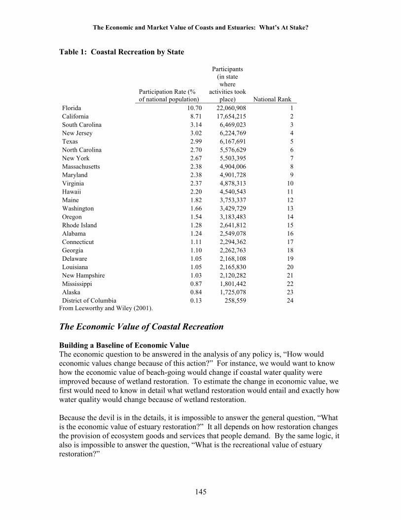
The Economic and Market Value of Coasts and Estuaries: What’s At Stake?
145
Table 1: Coastal Recreation by State
Participation Rate (% of national population)
Participants (in state where
activities took place) National Rank
Florida 10.70 22,060,908 1
California 8.71 17,654,215 2
South Carolina 3.14 6,469,023 3
New Jersey 3.02 6,224,769 4
Texas 2.99 6,167,691 5
North Carolina 2.70 5,576,629 6
New York 2.67 5,503,395 7
Massachusetts 2.38 4,904,006 8
Maryland 2.38 4,901,728 9
Virginia 2.37 4,878,313 10
Hawaii 2.20 4,540,543 11
Maine 1.82 3,753,337 12
Washington 1.66 3,429,729 13
Oregon 1.54 3,183,483 14
Rhode Island 1.28 2,641,812 15
Alabama 1.24 2,549,078 16
Connecticut 1.11 2,294,362 17
Georgia 1.10 2,262,763 18
Delaware 1.05 2,168,108 19
Louisiana 1.05 2,165,830 20
New Hampshire 1.03 2,120,282 21
Mississippi 0.87 1,801,442 22
Alaska 0.84 1,725,078 23
District of Columbia 0.13 258,559 24 From Leeworthy and Wiley (2001).
The Economic Value of Coastal Recreation
Building a Baseline of Economic Value
The economic question to be answered in the analysis of any policy is, “How would economic values change because of this action?” For instance, we would want to know how the economic value of beach-going would change if coastal water quality were improved because of wetland restoration. To estimate the change in economic value, we first would need to know in detail what wetland restoration would entail and exactly how water quality would change because of wetland restoration. Because the devil is in the details, it is impossible to answer the general question, “What is the economic value of estuary restoration?” It all depends on how restoration changes the provision of ecosystem goods and services that people demand. By the same logic, it also is impossible to answer the question, “What is the recreational value of estuary restoration?”

The Economic and Market Value of Coasts and Estuaries: What’s At Stake?
146
While it is not possible to provide general estimates of the recreational value of restoration, we can provide a baseline of these values. A baseline gives us an idea of the size of the economic pie that is coastal recreational value. Three important policy questions then follow from our understanding of the size of the economic pie. First, “How is the pie distributed around the country? Are there coastal and estuary areas that are particularly valuable for recreation?” Second, “How does our investment in coastal recreation compare to the economic value of this recreation?” Third, “How do our policies change the size of the pie?”
Understanding and Estimating Recreational Values
Coastal and marine recreation generates value for participants, revenues for local businesses that support these activities, and taxes for various levels of government. The economic impact of coastal recreation usually is assessed by examining how much money visitors contribute to the local economy through spending related to access, equipment, and goods and services (e.g., ice and bait). Commonly, the focus of market-based studies is on gross expenditures, with fewer studies focusing on profits or taxes. The economic value of coastal recreation is more difficult to determine. Economic value represents the value visitors place on the coastal and estuary resources, beyond what they have to pay to access these resources. As discussed in Chapter 1, the economic value of recreation has two components: use value and non-use value. Use values represent the economic value associated with the active use of a coastal recreational resource; non-use values represent the willingness to pay, by society or an individual, to protect a coastal resource that may never be used by those who express this willingness to pay. Non-use values include the willingness to pay to know that the coast exists (existence value), the willingness to pay to guarantee the option to possibly visit the coast in the future (option value), and the willingness to pay to guarantee that future generations have the opportunity to visit the coast (bequest value). While the literature recognizes economic values that accrue to both users (use values) and non-users (non-use values), we focus only on those values enjoyed by visitors to the coast as part of their use of the coast. The economic use value of recreation can be visualized by considering the demand for recreational activity days (Figure 1). All things being equal, visitors who can enjoy access to the coast at lower costs (e.g., people who live near the coast or live in states with protected public access) are likely to visit the coast more frequently than those who face higher costs. Figure 1 shows how many visits one would take at different costs of access. Another way to think of this figure is to turn it upside-down. A visitor only travels to the coast if the value they place on the coast is equal to or greater than the cost of access. Figure 2 shows the same relationship as Figure 1, but now we can interpret the figure as a map of the willingness to pay for each additional trip as a function of the number of trips taken. This willingness to pay for each additional trip is known as the “marginal willingness” to pay for recreation. The visitor keeps taking additional trips to the coast as long as the value of that additional trip is greater than or equal to the cost of that trip. If a visitor could take only one trip each year, they would place a high value on this trip. As the visitor takes more trips, the value they place on each trip declines slightly (principle of “diminishing marginal returns”). When the marginal value of a trip

The Economic and Market Value of Coasts and Estuaries: What’s At Stake?
147
is no longer greater than or equal to the cost of the trip, the visitor stays home or uses the day for some other type of activity.
Figure 1: Activity Days as a Function of Accessing the Coast
In Figure 2, Area A represents the cost of accessing the coast. This represents expenditures on the part of the visitor (e.g., for gas, parking, and possibly accommodations). These expenditures generate economic impact,2 but they do not represent value to the visitor. Imagine that we prohibit access by the visitor to the coast. The visitor simply keeps the money they would have spent on the trip and spends it elsewhere. These expenditures are retained. The value to the visitor of the recreational opportunity is the economic value they would lose if the recreational opportunity were eliminated; i.e., the amount they would be willing to pay, above what they pay in expenditures, to protect their ability to visit the coast. Area B, known as the consumer’s surplus, represents conceptually the value of the recreational activity, beyond any expenditures. Economists use the area to estimate the value of the activity because the willingness to pay for each trip, while declining, is additive across trips. The enjoyment of the second trip is added to the enjoyment of the first.
2 When expenditures exceed the actual costs of providing services (i.e., there is a profit), the producer or retailer is said to enjoy a net benefit. This is a true benefit to society, but we do not cover producer benefits in this chapter.
Cost of Access
Act
ivit
y D
ays
(Vis
its)
/yea
r
AD
i
Ci

The Economic and Market Value of Coasts and Estuaries: What’s At Stake?
148
Figure 2: The Marginal Willingness to Pay for an Activity
Figure 2 highlights two important issues associated with the value of recreational activities. First, consumers with lower costs of accessing the coast enjoy higher economic values from their coastal visits. As mentioned earlier, for many coastal recreational activities, the economic value of the resource may be large regardless of the level of spending associated with the activity. The published literature contains many examples where the economic values associated with coastal and marine resources exceed the market expenditures generated by these resources. Second, while we can estimate directly the number of visits taken to the coast and the costs of accessing the coast, we must deduce the size of the area under the demand curve. In the literature, two primary methods are used to estimate the economic use value (consumer surplus) of coastal recreation. Travel cost methods3 are used to estimate the trade-offs visitors make between travel costs (time and out-of-pocket expenses) and recreational opportunities. Travel cost methods use real visitor behavior to estimate the economic value of coastal recreation (the value the coastal visitor places on a recreational trip beyond what they have to pay), but because the method requires considerable variation in the travel costs faced by visitors, the method works best when applied to both residents and non-resident visitors (those living outside the immediate area). The literature review tables, later in this chapter, highlight the many applications of travel cost methods to beach-going, recreational fishing, diving, snorkeling, and wildlife viewing. Authors also use contingent methods (including contingent valuation, contingent ranking, and stated preference choice methods) to estimate values for coastal recreational use. Contingent methods rely on surveys to elicit from visitors their willingness to pay to use,
3 Travel cost methods include single and multiple site travel cost models and a variety of site choice models, including random utility models.
Co
st o
f A
cces
s (W
illi
ng
nes
s to
Pay
/Act
ivit
y D
ay
Ci
(Wil
lin
ges
s to
Pay
for
per
son
i)
A
B
Activity Days (Visits)/year Ci

The Economic and Market Value of Coasts and Estuaries: What’s At Stake?
149
protect, or avoid damage to coastal recreational resources or access. Both methods are used widely to estimate the value of coastal resources. Throughout the literature, economic values for recreation vary in terms of value type and units of value. There are two principal value types given in the literature—average value and marginal value. The (average use value)/(activity day) is equivalent to the consumer surplus (Area B) divided by the total number of trips taken over the course of a year or season. Marginal value, on the other hand, is the incremental value of one additional trip or activity day. Average values are always less than or equal to the marginal value of an activity day. In the summary of values from the literature below, we provide estimates of value/activity day and value/trip (both for individuals and households). Throughout our analysis, we focus primarily on value estimates for which we could deduce the value/activity day. Like all empirical statistical analyses, the validity of estimates from both methods varies with application and sample size. Valuation estimates from the literature are based on sample sizes that range from less than 100 to more than 1,000 observations. Some valuation estimates are derived from one-time surveys, and others rely on observations of repeated visits by panels of recreationists. In 1993, a Blue Ribbon Panel assembled by the National Oceanic and Atmospheric Administration developed criteria that ought to be met by contingent method studies in order to ensure the validity of economic valuation estimations using these methods (Arrow et al. 1993). These criteria, however, require expensive and extensive surveys and are rarely met in practice. No such criteria have been developed explicitly for the travel cost methods.
Using Values from the Literature: Benefits Transfer and Value Ranges
Benefits Transfer
In a few cases, nationwide studies have been undertaken to estimate the economic value of an environmental service (e.g., Viscusi et al. 2004 or Arrow et al. 1993). Value estimates for coastal recreation, however, are available only for relatively isolated, local or semi-regional examples. We need to draw from this geographically well-specified literature to better understand the potential economic value of coastal and estuarine restoration at a more national level.
Benefits transfer (or more appropriately value estimate transfer) generally refers to the practice of using value estimates from the literature for new policy applications. Benefit transfer techniques fall into two basic categories. In the first category, value estimates from the literature are applied to the new policy site application by adjusting for differences in quality or accessibility at the new location compared to the previous location(s). In the second category, the original valuation models are applied directly to the new policy application to generate new estimates of the potential economic value of the policy. In either case, the end result is usually a point estimate of value (i.e., one number) given with some margin of error.

The Economic and Market Value of Coasts and Estuaries: What’s At Stake?
150
Generally, there is no clear agreement in the literature that the application of benefits transfer methods are accurate or appropriate (see Wilson and Hoehn 2006). First, benefits transfer can only be as accurate as the original value transferred. As mentioned above, determining the accuracy of any single study is difficult. Studies in the literature often fail to provide information about the details of the research methods, sample characteristics, and findings. Second, the personal characteristics of recreationists and the physical characteristics of the recreation sites at both the original site and the policy site are usually only incompletely known, making attempts to adjust values or re-apply models difficult.
Benefits Ranges
In this chapter, we use a more conservative approach to draw conclusions about the potential economic value of coastal and estuary recreation from the literature. First, we attempt to provide a nearly exhaustive review of the peer-reviewed (and, when possible, technical) literature on the estimated economic value of recreational activities along the coasts and estuaries of the United States. In doing so, we hope readers will develop a good understanding of the range and magnitude of value estimates. We organize these valuation studies by recreation type and region to demonstrate how value estimates vary across uses and geography. All ranges and values are given in year 2005 U.S. dollars.
Estimating a Baseline of Value We develop a baseline of coastal recreational values by combining value estimates from the literature with regional and statewide estimates of user activity from the National Survey on Recreation and the Environment (NSRE). Throughout the rest of the paper, we present the value estimates from the literature and the user estimates from the NSRE at a state and regional level. For each region, we describe the level of use and the range of values associated with these activities, when estimated for that region or a nearby region. We also provide a range of potential value estimates for the region based on the literature and NSRE. We encourage readers to consider these ranges of estimates as “ball park” figures that highlight the potential magnitude of economic values. For each state or region, readers should use the data and literature presented to further explore and research the way in which these values are estimated.
Coastal Recreation The NSRE estimates statewide participation for 19 categories of coastal recreation. Table 2 provides a breakdown of activity days for each category of coastal and estuarine recreation, by state. Unless otherwise indicated, all activities take place on or in saltwater, including mixed freshwater/saltwater in tidal portions of rivers and bays. Of the 19 categories of recreation covered by the NSRE, the economic literature provides good data on the best economic value estimates for five recreational types: beach-going, recreational fishing, scuba diving, snorkeling, and bird and wildlife viewing. In all cases, tens of millions of activity days are devoted to coastal recreation. In this section, we examine the estimated economic values associated with these recreational activities and

The Economic and Market Value of Coasts and Estuaries: What’s At Stake?
151
provide state-level estimates of the potential economic benefit of these coastal uses. As always, readers are encouraged to dig deeper into the literature to find estimates of value that are most appropriate for the coastal areas of interest.
Beach-Going
The economic literature provides more than 30 estimates of the value of beach-going in the United States. Each year, approximately 853 million days are devoted to beach-going in the United States (Leeworthy and Wiley 2001). Of course, a visitor can undertake many activities while at the beach, such as swimming, sunbathing, collecting seashells, walking, jogging, viewing birds or other wildlife, or any number of other activities. This category is broad and should not be added to other more specific beach-related activities, to avoid double counting. The NSRE lists separately swimming, surfing, birdwatching, wildlife viewing, and wind surfing. The NSRE also includes as a category waterside activities, which captures all activities listed above for waterside coastal areas that are not beaches.

The Economic and Market Value of Coasts and Estuaries: What’s At Stake?
152
Table 2: Number of Annual Activity Days (millions) for Beach-Related Recreation
in the United States (1999–2000)
Beach
Visitation
Visiting
Waterside Swimming Surfing Windsurfing
Far-Western U.S.
Alaska 7.766 5.441 0.897 0 0
Hawaii 101.149 3.781 92.708 26.909 *
Western Continental U.S.
California 151.429 20.683 94.573 22.633 *
Oregon 13.789 2.309 5.161 * *
Washington 19.309 4.236 4.89 * *
Gulf-shore Southern U.S.
Alabama 11.842 3.65 8.203 * *
Florida (both coasts) 177.153 22.59 161.098 10.257 0.524
Louisiana 4.042 7.05 4.59 * *
Mississippi 8.679 1.317 6.739 * *
Texas 35.239 3.975 29.59 * *
Southeastern U.S.
Georgia 8.483 4.115 9.678 * 0
North Carolina 27.936 4.164 27.497 3.102 *
South Carolina 33.302 2.811 29.239 * *
Virginia 18.749 8.274 15.481 * *
Northeastern U.S.
Connecticut 14.065 2.408 12.774 0 *
Delaware 12.877 * 9.765 * *
District of Columbia * * * 0 0
Maine 16.159 4.3 13.513 * *
Maryland 18.696 5.894 18.351 * *
Massachusetts 28.681 2.925 31.66 * *
New Hampshire 8.126 1.985 8.374 * *
New Jersey 40.881 4.575 37.433 * *
New York 29.225 3.743 28.972 * *
Rhode Island 17.865 3.31 19.68 * *
Nationwide*
853 158 750 76 5.8
Adapted from Leeworthy and Wiley (2001).* Nationwide totals differ from the sum of state totals due to statistical aggregation.
The literature provides value estimates for beach-going in 11 states (Table 3). Values, estimated using both travel cost and contingent valuation methods, range from a low of just $0.07/trip in Delaware, Maryland, and New Jersey to highs of well over $70/activity day in California and Florida. As mentioned before, beach values can vary in the literature for a number of reasons, including the methods used to estimate values, whether visitors were residents or non-residents, the number of visitors surveyed, and other statistical properties of the analysis. Beach value also can vary because the quality of the beach-going experience and the average number of trips taken per individual per year varies across the country. Because of the principle of diminishing returns, the average and marginal value of a beach day could be lower (all things being equal) in areas in which visitors may make many trips.

The Economic and Market Value of Coasts and Estuaries: What’s At Stake?
153
Table 3: Literature Review of Coastal Beach Visitation Studies for the United
States
Beach Visitation
Author and Date
Consumer
Surplus/ Activity
Day Study Methodology
Far-Western U.S.
Hawaii Moncur, 1975 $1.60 - $6.25 TC
Western
Continental U.S.
California Dornsbusch et al. 1986 $11.99 TC
California Dornsbusch et al. 1987 $14.85 - $15.81 /trip TC
California Leeworthy et al. 1990 $1.72 - $8.04 CVM (four beaches)
California Leeworthy and Wiley, 1993 $12.19, $27.43, $77.61 TC (three beaches)
California King, 2001 $25.78 - $33.72 /household/day TC (during high season)
California Lew and Larson, 2005 $11.13/trip TC, RUM
Gulf-shore
Southern U.S.
Florida (both coasts) USACE, 1981 $3.69/trip TC
Florida (both coasts) Curtis and Shows, 1982 $4.48/trip CVM
Florida (both coasts) Curtis and Shows, 1984 $8.56/trip CVM
Florida (both coasts) Bell, 1986 $3.12 CVM
Florida (both coasts) Bell and Leeworthy, 1986 $2.46(residents) - $2.73(tourists) CVM
Florida (both coasts) Bell and Leeworthy, 1986 $19.23(residents) - $55.11(tourists) TC
Florida (both coasts) Bell and Leeworthy, 1990 $63.74 TC (tourists; Saltwater Beach use)
Florida (both coasts) Bell, 1992 $2.99 CVM (tourists)
Florida (both coasts) Bell and Leeworthy, 1990 $73.84 TC (Saltwater Beach use)
Florida (both coasts) USACE, 1993 $3.24/trip TC
Florida (both coasts) Leeworthy and Wiley, 1994 $22.28-$25.18 and $83.62-$92.67 TC (two beaches)
Florida (both coasts) Leeworthy and Bowker, 1997 $95.85 (winter) - $120.74 (summer)
TC (beach use; non-residents)
Southeastern U.S.
North Carolina Bin et al. 2004 revised 2005 $11.98 - $84.49 (mean) TC, RUM
Northeastern U.S.
Delaware Parsons et al. 1999 $0.07 - $12.70/trip* TC, RUM (6 beaches)

The Economic and Market Value of Coasts and Estuaries: What’s At Stake?
154
Beach Visitation
Author and Date
Consumer
Surplus/ Activity
Day Study Methodology
Maine Huang and Poor, 2004 $3.61 /household /day* CVM, DC (conjoint, fees)
Maryland Parsons et al. 1999 $0.07 - $12.70/trip* TC, RUM (6 beaches)
Massachusetts Hanemann, 1978 $1.04 TC
Massachusetts Binkley and Hanemann, 1978 $7.29 /household/trip CVM
Massachusetts Meta Systems, 1985 $20.32 TC (Boston beaches)
Massachusetts McConnell, 1992 $1.05 - $1.70 TC
Massachusetts Kline and Swallow, 1998 $5.36 CVM, DC (fees)
New Hampshire Huang and Poor, 2004 $3.61 /household /day* CVM, DC (conjoint, fees)
New Jersey Leeworthy and Wiley, 1991 $31.45 TC
New Jersey Parsons et al. 1999 $0.07 - $12.70/trip* TC, RUM (6 beaches)
Rhode Island McConnell, 1977 $1.42 - $6.43 CVM (6 beaches)
Rhode Island McConnell and Weaver, 1977 $5.74 CVM (working paper)
Coastal States for which no estimates are available do not appear in this Table.
Consumer Surplus values for one Activity Day unless otherwise noted.
TC = Travel Cost Method; RUM = Random Utility Model; CVM = Contingent Valuation Method
* Indicates loss due to beach closure
To estimate the annual statewide value of beach-going, we multiply the activity day estimates from the NSRE by a low and high estimate of the economic use value per person per day derived from the literature. As mentioned before, we provide ranges for each major region of the country. For most regions we use a high value of $50/activity day. The exceptions are Hawaii, where only one study appears in the literature that estimates the value of a beach day, and the northeastern United States, where value estimates are consistently lower than in other parts of the country. The low value for Hawaii may be an artifact of the one study considered, but also could result from the fact that resident Hawaiians take many visits to the beach. The bulk of beach-going activity in the United States occurs in the year-round destinations of Florida, California, and Hawaii (Table 4). The number of activity days devoted specifically to beach-going far exceeds other types of waterside activities and closely mirrors the number of visitors that went to the coast to swim (except for the western United States and Alaska, where the proportion of swimmers was the lowest). Based on values from the literature and estimates of beach activity days from the NSRE, beach-going in the United States is likely to generate tens of billions of dollars in economic use value annually (Table 4). We estimate that the economic use value of beach recreation at California beaches lies between $1.5 billion and $7.5 billion annually. Similarly, we estimate the economic use value of beach recreation in Florida to be between $886 million and just under $9 billion annually. Elsewhere around the country, beach recreation generates more than $100 million in annual use value in 13 coastal

The Economic and Market Value of Coasts and Estuaries: What’s At Stake?
155
states. The areas of highest value are concentrated in the western continental states, Texas, and the southeast and mid-Atlantic states. Strictly speaking, it is inappropriate to add these values across states, because a small fraction of activity days could have been undertaken at different states on the same day. If we assume that this potential for double counting is small, then we can estimate roughly that the value of beach recreation across the country is likely to be between a low of just under $6 billion and a high of nearly $30 billion annually.
Table 4: Estimated Annual Statewide Values of Beach-Going in the United States
($US millions)
Statewide Annual
Visitation (millions of
activity days)
Total Statewide Value Estimates
(rounded, millions $2005)
LOW HIGH
Far-Western U.S. $2/activity day $6/activity day
Alaska 7.766 $16 $47
Hawaii 101.149 $202 $607
Western
Continental U.S.
$10/activity day $50/activity day
California 151.429 $1,514 $7,571
Oregon 13.789 $138 $689
Washington 19.309 $193 $965
Gulf-shore
Southern U.S. $5/activity day $50/activity day
Alabama 11.842 $59 $592 Florida (both coasts) 177.153 $886 $8,858
Louisiana 4.042 $20 $202
Mississippi 8.679 $43 $434
Texas 35.239 $176 $1,762
Southeastern U.S. $20/activity day $50/activity day
Georgia 8.483 $170 $424
North Carolina 27.936 $559 $1,397
South Carolina 33.302 $666 $1,665
Virginia 18.749 $375 $937
Northeastern U.S. $5/activity day $20/activity day
Connecticut 14.065 $70 $281
Delaware 12.877 $64 $258 District of Columbia * * *
Maine 16.159 $81 $323
Maryland 18.696 $93 $374
Massachusetts 28.681 $143 $574
New Hampshire 8.126 $41 $163
New Jersey 40.881 $204 $818
New York 29.225 $146 $585
Rhode Island 17.865 $89 $357

The Economic and Market Value of Coasts and Estuaries: What’s At Stake?
156
Recreational Fishing
Recreational fishing also has been well-studied and numerous estimates of the use value of recreational angling are available in the literature, although most studies were conducted in the 1980s and early 1990s. Estimates of recreational fishing use values also are available through the Sportfishing Values Database (www.indecon.com/fish/) –a web-based database of value estimates and metadata for marine and freshwater sportfishing. We review 13 studies of marine recreational fishing in which estimates of the value of an activity day or trip are given (Table 5). In some cases original studies were not available, but values were provided in the Sportfishing Values Database. We indicate these articles by using the phrase “secondary data only” in the Methods column. Generally, estimates for the use value of a day of recreational fishing in the United States fall between $20 and $100 with high estimates of well over $145/activity day in Alaska (and higher estimates for the use value associated with trips). Value estimates from the Atlantic states also run consistently high.
Table 5: Literature Review of Coastal Recreational Fishing Studies for the United
States
Author and Date Consumer Surplus/ Activity Day Study Methodology
Far-Western U.S.
Alaska Jones and Stokes, 1987 $4.60 - $33.90 /trip
TC, RUM (secondary data only; private boat, rental boat and shore, Halibut, King Salmon, Silver Salmon, other species)
Alaska Wegge et al. 1988 $69.94/trip RUM (secondary data only)
Alaska Hausman et al. 1995 $188.02/trip TC (residents)
Alaska Hamel et al. 2000 $99.39 TC, CVM (residents; Salmon, Halibut from private boat)
Alaska Hamel et al. 2000 $119.62
TC, CVM (residents and non-residents; Salmon, Halibut from private boat)
Alaska Hamel et al. 2000 $146.14
TC, CVM (non-residents; Salmon, Halibut from charter boat)
Western
Continental U.S.
California Huppert and Thomson, 1984 $33.54/trip
TC (both residents and non-resident; travel valued at 1/3 wage rate)
California Hanemann et al. 1986 $16.21 TC (shore fishing; boat owner)
California Hanemann et al. 1986 $29.57 TC (shore fishing; non-boat owner)
California Wegge et al. 1986 $44.33/trip
CVM (charter boat; Pacific Mackerel, Kelp Bass, Rockfish)
California Wegge et al. 1986 $24.33 - $43.34 (trips < or = 1 day)
TC, (charter boat; boat owner; residents and non-residents)

The Economic and Market Value of Coasts and Estuaries: What’s At Stake?
157
Author and Date Consumer Surplus/ Activity Day Study Methodology
California Wegge et al. 1986 $30.04 - $96.53 (trips < or = 1 day)
TC, (charter boat; non boat owner; residents and non-residents)
California Wegge et al. 1986 $29.55 CVM (private boat, rental; residents and non-residents)
California Wegge et al. 1986 $14.78
CVM (private boat, shore fishing; residents and non-residents)
California Wegge et al. 1986 $59.10 CVM (private boat; residents and non-residents)
California Wegge et al. 1986 $35.30 TC (private boat; owner; residents and non-residents)
California Wegge et al. 1986 $29.10 TC (private boat; non-owner; residents and non-residents)
California Huppert, 1989 $110.41, $242.54, $535.76 / trip
TC, (residents; Salmon, Halibut; boat and shore)
California Kling and Herriges, 1995
$10.84 - $21.35 /undefined period
Unknown methodology (Shore fishing; residents)
California Kling and Herriges, 1995
$27.46-$44.45 /undefined period
Unknown methodology (Off-shore fishing; residents)
Oregon Row, R, 1985 $116.07/trip TC and RUM (secondary data only)
Washington Cruthfield and Schelle, 1978 $55.48 CVM (secondary data only)
Washington Row, R, 1985 $100.52/trip TC and RUM (secondary data only)
Gulf-shore
Southern U.S. Florida (both coasts) Bell et al. 1982 $82.90 CVM (Residents) Florida (both coasts) Bell et al. 1982 $61.86 - $77.00 CVM (Non-Residents) Florida (both coasts) Leeworthy, 1990 $81.33/trip TC (secondary data only)
Florida (both coasts)
McConnell & Strand, 1994 $113.03-$135.86
TC and RUM (non-residents; secondary data only)
Florida (Gulf coast) Bell, F.W., 1997 $66.70
TC (Residential Status Not Specified)
Florida (East coast) Bell, F.W., 1997 $100.64
TC (Residential Status Not Specified)
Texas Downing and Ozuna, 1996
$60.23-$407.29/trip CVM (Residents)
Southeastern U.S.
Georgia McConnell & Strand, 1994 $66.06-$70.12
TC and RUM (non-residents; secondary data only)
North Carolina Norton et al. 1983 $277.15/trip TC (residents; secondary data only)
North Carolina McConnell & Strand, 1994 $111.23-$114.81
TC and RUM (non-residents; secondary data only)

The Economic and Market Value of Coasts and Estuaries: What’s At Stake?
158
Author and Date Consumer Surplus/ Activity Day Study Methodology
South Carolina McConnell & Strand, 1994 $113.03-$114.44
TC and RUM (non-residents; secondary data only)
South Carolina Bockstael et al. 1986 $97.92 CVM (secondary data only)
Virginia Norton et al. 1983 $93.99/trip TC (residents; secondary data only; boat and shore)
Virginia McConnell & Strand, 1994 $64.01-$77.48
TC and RUM (non-residents; secondary data only)
Northeastern U.S.
Connecticut Norton et al. 1983 $207.26/trip TC (residents; secondary data only)
Delaware Norton et al. 1983 $407.29/trip TC (residents; secondary data only; shore fishing)
Delaware McConnell & Strand, 1994 $17.07-$18.51
TC and RUM (non-residents; secondary data only)
Maine Norton et al. 1983 $207.26/trip TC (residents; secondary data only)
Maryland McConnell & Strand, 1994 $44.67-$45.73
TC and RUM (non-residents; secondary data only)
Massachusetts Norton et al. 1983 $207.26/trip TC (residents; secondary data only)
New Hampshire Norton et al. 1983 $207.26/trip TC (residents; secondary data only)
New Jersey Norton et al. 1983 $407.29/trip TC (residents; secondary data only; shore fishing)
New Jersey McConnell & Strand, 1994 $54.03-$56.95
TC and RUM (non-residents; secondary data only)
New York Norton et al. 1983 $407.29/trip TC (residents; secondary data only; shore fishing)
New York McConnell & Strand, 1994 $96.35-$98.31
TC and RUM (non-residents; secondary data only)
Rhode Island Norton et al. 1983 $207.26/trip TC (residents; secondary data only)
DE, FL, GA, MD, NC, NJ, NY, SC, VA McConnell et al. 1993 $215.85
CVM (non-residents; secondary data only)
Coastal States for which no estimates are available do not appear in this Table.
Consumer Surplus values for one Activity Day unless otherwise noted.
TC = Travel Cost Method; RUM = Random Utility Model; CVM = Contingent Valuation Method
More than 21 million people fish at least once each year in the coastal United States. Combined, these anglers spend 259 million days fishing in marine and estuarine areas—far fewer than the number of days devoted to beach-going and fewer than the number of days devoted to birdwatching and other types of wildlife viewing. Fishing is highly concentrated in Florida and California. Low estimates for the annual economic use value of recreational fishing range from several hundred million dollars for most states to several billion dollars for Florida (Table 6). High estimates of recreational fishing use value exceed $1 billion annually for many states.

The Economic and Market Value of Coasts and Estuaries: What’s At Stake?
159
Table 6: Estimated Annual Statewide Values of Coastal and Estuary Recreational
Fishing in the United States ($US millions)
Statewide Annual
Visitation
(millions of
activity days)
Total Statewide Value Estimates (rounded,
millions $2005)
LOW HIGH
Far-Western U.S. $30/activity day $145/activity day
Alaska 10.588 $318 $1,535
Hawaii 16.071 $482 $2,330
Western Continental U.S. $25/activity day $100/activity day
California 20.318 $508 $2,032
Oregon 2.78 $70 $278
Washington 4.4 $110 $440
Gulf-shore Southern U.S. $60/activity day $100/activity day
Alabama 4.217 $253 $422
Florida (both coasts) 56.285 $3,377 $5,629
Louisiana 12.486 $749 $1,249
Mississippi 4.663 $280 $466
Texas 16.425 $986 $1,643
Southeastern U.S. $60/activity day $100/activity day
Georgia 3.003 $180 $300
North Carolina 10.381 $623 $1,038
South Carolina 6.097 $366 $610
Virginia 7.72 $463 $772
Northeastern U.S. $15/activity day $100/activity day
Connecticut 7.792 $117 $779
Delaware 8.08 $121 $808
District of Columbia * * *
Maine 2.967 $45 $297
Maryland 11.06 $166 $1,106
Massachusetts 8.098 $121 $810
New Hampshire 1.918 $29 $192
New Jersey 14.687 $220 $1,469
New York 14.523 $218 $1,452
Rhode Island 4.806 $72 $481
Birdwatching and Whale Watching
Each year nearly 15 million people spend nearly 900 million days enjoying bird viewing along U.S. shores; more than 13 million people spend 341 million days watching other marine and coastal wildlife. Despite the popularity of bird and wildlife viewing, the literature has given only scant attention to the economic valuation of marine and estuarine wildlife viewing in the United States (although a substantially larger literature exists for international studies of the economic value of wildlife viewing). Where wildlife viewing has been studied for marine species in the United States, the values per activity day are usually high (Table 7). For instance, Colt (2001), based on a survey by McCollum and Miller (1994), estimated that in Alaska residents would have been willing

The Economic and Market Value of Coasts and Estuaries: What’s At Stake?
160
to pay $240 more than actual expenditures for a day of watching sea birds ($133 when birdwatching was only a secondary reason for their visit to the coast) and $228 for whale watching ($208 when whale watching was a secondary reason for the visit).
Table 7: Literature Review of Coastal and Marine Wildlife Viewing Studies for the
United States
Author and Date Consumer Surplus/ Activity Day
Study Methodology
Far-Western U.S.
Alaska McCollum and Miller, 1994 in Colt 2001
Seabirds: $133 - $240 Whales: $208 - $228 Unreported
Western Continental
U.S.
California Hall et al. 2002 $6.78/family visit CVM (tidepool visits)
Gulf-shore Southern
U.S.
Florida (both coasts) Leeworthy and Bowker, 1997 $108.35 TC (Florida Keys)
Northeastern U.S.
New York Johnston et al. 2002 $63.80 TC
New England (whale watching)
Hoagland and Meeks, 2000
$62.50 - $70.40 TC
Because of the small number of valuation estimates in the literature, we use a single pair of conservative low and high estimated consumer surplus values/activity day ($10 and $100) to calculate the upper and lower bounds of the potential economic value of birdwatching and wildlife viewing in the United States. Because of the large number of days devoted in some part to watching birds and other marine and coastal wildlife, the low estimate of the use value of these activities exceeds $100 million for most coastal states and reaches a high estimate of several billion dollars annually for many states (Table 8).
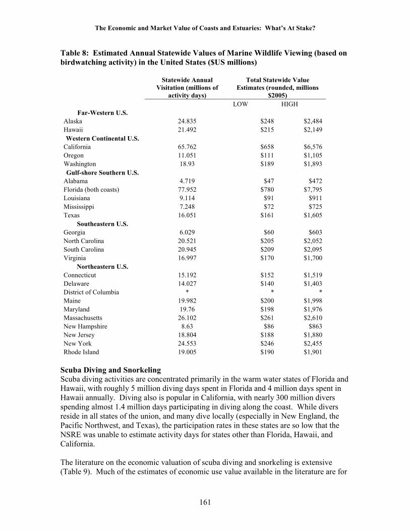
The Economic and Market Value of Coasts and Estuaries: What’s At Stake?
161
Table 8: Estimated Annual Statewide Values of Marine Wildlife Viewing (based on
birdwatching activity) in the United States ($US millions)
Statewide Annual
Visitation (millions of
activity days)
Total Statewide Value
Estimates (rounded, millions
$2005)
LOW HIGH
Far-Western U.S.
Alaska 24.835 $248 $2,484
Hawaii 21.492 $215 $2,149
Western Continental U.S.
California 65.762 $658 $6,576
Oregon 11.051 $111 $1,105
Washington 18.93 $189 $1,893
Gulf-shore Southern U.S.
Alabama 4.719 $47 $472
Florida (both coasts) 77.952 $780 $7,795
Louisiana 9.114 $91 $911
Mississippi 7.248 $72 $725
Texas 16.051 $161 $1,605
Southeastern U.S.
Georgia 6.029 $60 $603
North Carolina 20.521 $205 $2,052
South Carolina 20.945 $209 $2,095
Virginia 16.997 $170 $1,700
Northeastern U.S.
Connecticut 15.192 $152 $1,519
Delaware 14.027 $140 $1,403
District of Columbia * * *
Maine 19.982 $200 $1,998
Maryland 19.76 $198 $1,976
Massachusetts 26.102 $261 $2,610
New Hampshire 8.63 $86 $863
New Jersey 18.804 $188 $1,880
New York 24.553 $246 $2,455
Rhode Island 19.005 $190 $1,901
Scuba Diving and Snorkeling
Scuba diving activities are concentrated primarily in the warm water states of Florida and Hawaii, with roughly 5 million diving days spent in Florida and 4 million days spent in Hawaii annually. Diving also is popular in California, with nearly 300 million divers spending almost 1.4 million days participating in diving along the coast. While divers reside in all states of the union, and many dive locally (especially in New England, the Pacific Northwest, and Texas), the participation rates in these states are so low that the NSRE was unable to estimate activity days for states other than Florida, Hawaii, and California. The literature on the economic valuation of scuba diving and snorkeling is extensive (Table 9). Much of the estimates of economic use value available in the literature are for

The Economic and Market Value of Coasts and Estuaries: What’s At Stake?
162
diving on existing and proposed artificial structures, including sunken ships and other types of artificial reefs (see Pendleton 2005 for a review). Valuation estimates are generally consistent across the many site types and geographical locations. We use a low estimate of $15/activity day and a high estimate of $50/activity day to estimate the value of scuba diving in Florida, Hawaii, and California. Compared to other coastal recreational activities, the state-level economic value of scuba diving is modest, although it is likely to be locally significant at many exceptional dive areas (e.g., Key Largo, Catalina Island, and much of Hawaii). Low estimates do not exceed $100 million annually for any of the three states considered. High estimates do not exceed $300 million annually (Table 10).
Table 9: Literature Review of Coastal Scuba Diving Studies for the United States
Author and Date Consumer Surplus/ Activity Day Study Methodology
United States
All US National Parks Kaval and Loomis, 2003 $34.25
Western Continental
U.S.
California Leeworthy and Wiley, 2002 $13.78
(Benefit transfer, Santa Barbara and Ventura Counties)
California Leeworthy and Wiley, 2002 $41.35 - $42.95
(Channel Islands National Marine Sanctuary)
California Pendleton 2005 $110/day Ship diving on the Yukon
Pacific Coast Kaval and Loomis, 2003 $55.66
Gulf-shore Southern
U.S.
Gulf of Mexico Roberts et al. 1985 $350.49/year/diver CV (petroleum structures)
Gulf of Mexico Stoll and Ditton, 2002 $121.20/trip (secondary source; artificial reef)
Gulf of Mexico Stoll and Ditton, 2002 $157.20/trip (secondary source; natural reef)
Florida Milon, 1988 $30.02 - $44.22/year/diver
CV (fishing and diving on 7 artificial reefs)
Florida Milon, 1989 $4.63 - $131.88/year/diver
CV (fishing and diving on ships and steel debris)
Florida Bell et al. 1998 $11.36 TC (ships, reef balls, other structures)
Florida Bell et al. 1998
$3.62 - $4.40(residents); $6.51 - $7.96(visitors)
CV (ships, reef balls, other structures)
Florida Leeworthy et al. 2001
$4.02(residents) - $16.16(non-residents) (artificial reef)

The Economic and Market Value of Coasts and Estuaries: What’s At Stake?
163
Author and Date Consumer Surplus/ Activity Day Study Methodology
Florida Johns et al. 2003 $3.52(residents) - $14.47(visitors)
CV (maintain existing artificial reefs)
Texas Ditton and Baker, 1999 $49.53 - $83.48 CV (diving on artificial reefs)
Texas Ditton et al. 2001 $46.52 CV (diving on artificial reefs)
Northeastern U.S.
Northeast Region Kaval and Loomis, 2003 $18.96
Coastal States for which no estimates are available do not appear in this Table.
Consumer Surplus values for one Activity Day unless otherwise noted.
TC = Travel Cost Method; RUM = Random Utility Model; CVM = Contingent Valuation Method
Table 10: Estimated Annual Statewide Values of Scuba Diving in the United States
($US millions)
Statewide Annual
Visitation (millions of
activity days)
Total Statewide Value Estimates (rounded,
millions $2005)
LOW HIGH
Far-Western U.S.
Hawaii 4.251 $64 $213
Western
Continental U.S.
California 1.383 $21 $69
Gulf-shore Southern
U.S.
Florida (both coasts) 5.42 $81 $271
Significant snorkeling activity, like scuba diving, also is limited to Florida, Hawaii, and California. The range of values for snorkeling is similar to those for scuba diving, probably owing in part to the relatively low cost of snorkeling compared to diving (Table 11). Also possibly owing to this low cost, participation in snorkeling is between 3 and 6 times higher than scuba diving. As a result of these higher levels of activity, the economic use value of snorkeling is likely to be equal to or greater than similar estimates for scuba diving. We use a lower estimate of $10/activity day and a high estimate of $50/activity day to estimate the potential economic use value of snorkeling. While the lower bound estimates for the economic use values of snorkeling for the three states are similar to scuba diving, the upper bound estimates are significantly higher, exceeding $1 billion for Florida and Hawaii (Table 12).

The Economic and Market Value of Coasts and Estuaries: What’s At Stake?
164
Table 11: Literature Review of Coastal Snorkeling Studies for the United States
Author and Date Consumer Surplus/ Activity Day Study Methodology
United States
All US National Parks Kaval and Loomis, 2003 32.08 (resident and non-resident)
Western Continental
U.S.
Pacific Coast Kaval and Loomis, 2003 $31.58
Gulf-shore Southern
U.S.
Florida (both coasts) Leeworthy and Bowker, 1997 $118.96
(resident and non-resident)
Florida (both coasts) Leeworthy et al. 2001 $3.02(resident) - $8.37(non-resident) (artificial reef)
Florida (both coasts) Park et al. 2002 $130.59/trip (resident and non-resident)
Table 12: Estimated Annual Statewide Values of Snorkeling in the United States
($US millions)
Statewide Annual
Visitation (millions
of activity days)
Total Statewide Value Estimates (rounded,
millions $2005)
LOW HIGH
Far-Western U.S.
Hawaii 24.158 $242 $1,208
Western Continental U.S.
California 3.818 $38 $191
Gulf-shore Southern U.S.
Florida (both coasts) 23.956 $240 $1,198
Coastal Recreation Is Valuable. So What? The economic value of coastal recreation is indeed great. If we ignore the small effects of double counting for activities that take place in different states on the same day, we begin to get a picture of the economic use value of coastal recreation from a regional and national perspective. Table 13 provides a summary of regional and national values for beach-going, recreational fishing, wildlife viewing, scuba diving, and snorkeling. The value of beach-going, recreational fishing, and wildlife viewing are each greater than $4 billion annually, and the value may be nearly $50 billion annually for wildlife viewing and nearly $30 billion for beach-going and recreational fishing. The possibility of double counting makes it inappropriate to add the values of all activities together. Nevertheless, if we recognize that there is likely to be little double counting for beach-going and recreational fishing, we can add these two activities together to see that the potential economic value of beach-going and angling combined are likely to be between $16

The Economic and Market Value of Coasts and Estuaries: What’s At Stake?
165
billion and $56 billion. Adding the value of other activities to this total pushes the economic value of coastal recreation well beyond $20 billion to $60 billion. It is hard to compare the economic use value of coastal recreation to other numbers in the economy, because we rarely make the effort to calculate the use value of market goods and services. Estimating use values is time-consuming and difficult, even for market goods for which we have abundant market price and demand data. As a result, economists usually fall back on market data because they at least reveal the true willingness of society to pay for the last unit of a good or service, and therefore they provide a lower bound estimate of the value of these goods and services. Coastal recreation, on the other hand, often occurs largely in the absence of fully functioning markets. Coastal access often is free or made available at fixed prices (e.g., the cost of municipal beachside parking). Because there is no market for most types of coastal recreation, we cannot rely on market prices. But the question remains, is $20 billion to $60 billion in economic use value a lot? Let’s compare this figure to sectors for which we have market data. The total gross state product (GSP) in 2004 for all ocean sector goods and services recorded by the NOEP was $138 billion. Marine minerals generated $19.6 billion in GSP for 2004, and all marine-related tourism and recreation generated $69.7 billion. Commercial fishing is a marine market sector so important that an entire government agency (NOAA’s National Marine Fisheries Service) is charged with its monitoring and management. In 2004, the top 10 commercial fish species had a landed value of just over $2 billion (National Ocean Economics Program), and the value of all reported landings for more than 416 species of fish and shellfish was $3.5 billion. So, yes, $20 billion to $60 billion is a lot of economic value. Unfortunately, the non-market nature of the value of recreation means that this economic value often is overlooked in coastal and estuarine policymaking.
Table 13: Estimated Annual Value of Select Coastal Activities in the United States
($ millions)
Beach Visitation
Recreational
Fishing
Wildlife
Viewing
SCUBA
Diving Snorkeling
Low High Low High Low High Low High Low High
Far-Western
U.S. $218 $653 $800 $3,866 $463 $4,633 * * * *
Western
Continental
U.S. $1,845 $9,226 $687 $2,750 $957 $9,574 $21 $69 $38 $191
Gulf-shore
Southern
U.S. $1,185 $11,848 $5,645 $9,408 $1,151 $11,508 $81 $271 $240 $1,198
Southeastern
U.S. $1,769 $4,424 $1,632 $2,720 $645 $6,449 * * * *
Northeastern
U.S. $933 $3,732 $1,109 $7,393 $1,661 $16,606 * * * *
U.S. Total $5,950 $29,883 $9,873 $26,136 $4,877 $48,770 $102 $340 $278 $1,389

The Economic and Market Value of Coasts and Estuaries: What’s At Stake?
166
Knowing the value of coastal and marine recreation can help Congress better determine how much the federal government should spend to protect, monitor, and enhance coastal and estuarine recreational activities. Unfortunately, government investment in coastal protection has been consistently low. In 2006, total federal spending on ocean-related activities was only $8.2 billion (NOEP). The budget for NOAA, the principal marine and coastal management agency, was just under $1.4 billion—only 24% of the low value of beach recreation and only 5% of the high value of beach-going, 5% of the high value of recreational fishing, and 3% of the high value of marine bird and wildlife viewing. Of course, federal spending on coastal recreation is only a small part of total government spending on ocean activities. The relative annual investment in coastal and estuarine recreation is likely to be a small fraction of a percent of its total value. While coastal recreation occurs in every coastal state, recreational value is concentrated in different regions (Figure 1). From a national perspective, beach going recreation generates the greatest value in the western continental states and Florida, recreational fishing is particularly valuable in the Gulf States and Florida, and wildlife viewing is most valuable in the northeastern states. Decisions about the distribution of funds to protect and enhance coastal recreation should take these value distributions into account.
Recreational Use Value and Habitat Restoration
Accounting for the economic use value of coastal and estuary recreation gives us our first nationwide glimpse at the potential value of habitat restoration for at least one user group—everyday people who enjoy the coast and coastal waters. Many types of coastal recreation depend on ecosystem and environmental conditions. For instance, recreational fishing success has been linked to environmental conditions (see Lipton and Hicks 2003; Lipton and Strand 1997). Beach values and attendance have been linked to fecal indicator bacteria (see for example Bockstael, Hanemann, and Kling 1987; Bockstael, McConnell, and Strand 1989; Freeman 1995; Hayes, Tyrrell, and Anderson 1992; Murray, Sohngen and Pendleton 2001; Smith, Zhang, and Palmquist 1997), birdwatchers and wildlife viewers are known to place a direct value on being able to see certain species (e.g., McCollum and Miller, 1994 in Colt 2001; Johnston et al. 2002; Hoagland and Meeks 2000). Even divers have been shown to prefer sites with higher fish abundances and coral diversity (e.g., Pendleton 1994). The values estimated here represent the current value of coastal recreation, under current environmental conditions which, in many cases, are quite degraded. Because many coastal recreational activities depend on environmental conditions, coastal restoration could increase the values presented in this chapter. Understanding the exact magnitude of economic improvement that could come from coastal restoration would require a detailed understanding of the proposed restoration with an equally detailed ability to predict how behavior, use, and values would change as a result of restoration. Nevertheless, we can use this baseline to place rough economic values on potential improvements in coastal and estuary habitats. For instance, if we could improve the value of beach-going opportunities in the western continental United

The Economic and Market Value of Coasts and Estuaries: What’s At Stake?
167
States by a mere 1%, the annual economic value of that improvement would be between $18 million and $92 million annually. At a 3% discount rate (the rate mandated for use by the Office of Budget and Management, 2007 Discount Rates for OMB Circular No. A-94) the capitalized value of that return would be between $600 million and $3 billion—just for beach-going—just in California, Oregon, and Washington. Readers are encouraged to use the data and literature presented in this chapter to consider the potential economic value that could come from improved management of coastal and estuarine resources in their state and region, and nationwide.
Table 14: Links Between Environmental Conditions and Coastal Recreation
Activity Link to coastal environmental conditions
Recreational Fishing Water quality (O2), nursery habitat, fish abundance Beach Going (swimming) Water quality (bacteria), harmful algal blooms Bird and Wildlife Viewing Fish (for forage); bird and wildlife abundance,
diversity, and rare species; habitat SCUBA/Snorkeling Fish abundance, coral cover
CASE STUDY: Economic Value in the Sunshine State
According to the NSRE data, Florida ranks first among the nation’s destinations for Americans who swim, fish, dive, and otherwise enjoy the state’s many beaches, coastal wetlands, and shores. Florida’s 770 miles of coastline4 (NOAA 1975), including the Gulf, Atlantic, and Caribbean coasts, is the most visited in the nation, with almost one in 10 Americans visiting the Florida coasts in 2000 (more than 22 million visitors overall) (Leeworthy and Wiley 2001) Visitors to Florida and local Floridians visit shores and beaches to swim, sunbathe, watch wildlife (especially birds), photograph scenery, boat, fish, and dive. The NSRE provides estimates for the number of participants and the number of days of participation for a variety of coastal activities in Florida.
4 There are many different ways to measure the useable coastline. NOAA’s 1975 figure may not agree with other measures of the Florida coast.

The Economic and Market Value of Coasts and Estuaries: What’s At Stake?
168
Table 15: Annual Participation in Coastal Recreational Activities in Florida
(1999/2000)
Activities
Participants (in state where
activities took place,
millions)
Activity
Days (millions)
Beach-going 15.246 177.153
Bird Watching 3.373 77.952
Canoeing 0.019 n/a
Fishing 4.698 56.285
Hunting 0.072 *
Kayaking 0.338 n/a
Motorboating 3.337 46.624
Other Wildlife 2.846 50.264
Personal Watercraft 1.626 14.54
Photography Scenery 3.92 96.591
Rowing 0.153 n/a
SCUBA 0.802 5.42
Snorkeling 2.866 23.956
Swimming 14.033 161.098
Waterside 1.801 22.59
Waterskiing 0.613 4.475 * Too few to estimate N/A data not collected
Of these many activities, we have attempted to estimate the potential statewide economic use value of beach-going, recreational fishing, bird and wildlife viewing, snorkeling, and scuba diving. Even our most conservative estimates find a value of more than $5 billion annually for coastal recreation in Florida
Table 16: The Potential Range of Economic Use Values for the Florida Coast
Activities Low Estimate High Estimate
Beach-going $886 $8,858
Bird and Wildlife Viewing $780 $7,795
Recreational Fishing $3,377 $5,629
Snorkeling $240 $1,198
Scuba Diving $81 $271
Total Potential Economic Use Value $5,364 $23,751

The Economic and Market Value of Coasts and Estuaries: What’s At Stake?
169
References
Arrow, K., R. Solow, P. Portney, E. Leamer, R. Radner and H. Schuman. 1993. Report of
the NOAA panel on contingent valuation. Volume 58: 4601-14. Bell, F. W. 1986. "Economic policy issues associated with beach renourishment." Policy
Studies Review 6(2): 374-381. Bell, F. W. 1992. Actual and potential tourist reaction to adverse changes in recreational
coastal beaches and fisheries in Florida. Florida Sea Grant College. Bell, F. W., M. A. Bonn and V. R. Leeworthy. 1998. Economic impact and importance of
artificial reefs in Northwest Florida. National Oceanic and Atmospheric Administration and Office of Fisheries Management and Assistance Service, Florida Department of Environmental Protection.
Bell, F. W. and V. R. Leeworthy. 1986. An economic analysis of the importance of
saltwater beaches in Florida. Florida Sea Grant College. Bell, F. W. and V. R. Leeworthy. 1990. "Recreational demand by tourists for saltwater
beach days." Journal of Environmental Economics and Management 18(3): 189-205.
Bell, F. W., P. E. Sorensen and V. R. Leeworthy. 1982. The economic impact and
valuation of saltwater recreational fisheries in Florida. Florida Sea Grant College. Bin, O., C. Landry, C. Ellis and H. Volgelsong. 2005. "Some consumer surplus estimates
for North Carolina beaches." Marine Resource Economics 20(2): 145-61. Binkley, C. S. and W. M. Hanemann. 1978. The recreation benefits of water quality
improvement: analysis of day trips in an urban setting. U.S. Environmental Protection Agency, Office of Research and Development, Office of Health and Ecological Effects.
Bockstael, N., A. Graefe, I. Strand and L. Caldwell. 1986. Economic analysis of artificial
reefs: a pilot study of selected valuation methodologies. Artificial Reef Development Center: Volume 6.
Bockstael, N., W. M. Hanemann and C. Kling. 1987. "Estimating the value of water
quality improvements in a recreational demand framework." Water Resources Research 23(5): 951-960.
Bockstael, N., K. McConnell and I. E. Strand. 1989. "Measuring the benefits of
improvements in water quality: the Chesapeake Bay." Marine Resource Economics 6: 1-18.

The Economic and Market Value of Coasts and Estuaries: What’s At Stake?
170
Colgan. 2004. "Employment and wages in the ocean economy of the United States." Monthly Labor Review.
Colt, S. 2001. The economic importance of healthy Alaska ecosystems. Anchorage,
Alaska Conservation Foundation and Institute of Social and Economic Research, University of Alaska Anchorage.
Crutchfield, J. A. and K. Schelle. 1978. An economic analysis of Washington ocean
recreational salmon fishing with particular emphasis on the role played by the charter vessel industry. Pacific Fishery Management Council, NMFS.
Curtis, T. D. and E. W. Shows. 1982. Economic and social benefits of artificial beach
nourishment -- civil works at Delray Beach. Tampa, Florida Department of Natural Resources, Division of Beaches and Shores and Department of Economics, University of South Florida, Tampa.
Curtis, T. D. and E. W. Shows. 1984. Economic and social benefits of artificial beach
nourishment -- civil works in Northeast Florida. Tampa, Florida Department of Natural Resources, Division of Beaches and Shores and Department of Economics, University of South Florida, Tampa.
Ditton, R. B. and T. L. Baker. 1999. Demographics, attitudes, management preferences,
and economic impacts of sport divers using artificial reefs in offshore Texas waters. College Station, Human Dimensions of Fisheries Research Lab, Department of Wildlife and Fisheries Sciences, Texas A&M University: 44p.
Ditton, R. B., C. B. Thailing, R. Riechers and H. Osburn. 2001. The economic impacts of
sport divers using artificial reefs in Texas offshore waters. College Station, Department of Wildlife and Fisheries Sciences, Texas A&M University: 18p.
Dornbusch, D. 1986. OCS impacts on California coastal recreation: detailed methodology
Los Angeles, U.S. Department of the Interior, Minerals Management Service: Volumes 1-3.
Dornbusch, D. and A. E. Systems. 1987. Impacts of Outer Continental Shelf (OCS)
development on recreation and tourism. Los Angeles, U.S. Department of the Interior, Minerals Management Service: Volume 3.
Downing, M. and T. J. Ozuna. 1996. "Testing the Reliability of the Benefit Function
Transfer Approach." Journal of Environmental Economics and Management 30: 316-322.
Freeman, A. M. 1995. "The benefits of water quality improvements for marine
recreation: a review of the empirical evidence." Marine Resource Economics 10(4): 385-406.

The Economic and Market Value of Coasts and Estuaries: What’s At Stake?
171
Hall, D. C., J. V. Hall and S. N. Murray. 2002. "Contingent valuation of Marine Protected Areas: Southern California rocky intertidal ecosystems." Natural Resource Modeling 15(3): 335-368.
Hamel, C., M. Herrmann, T. S. Lee and K. R. Criddle. 2000. An economic discussion of
the marine sport fisheries in Lower Cook Inlet. Tenth meeting of the International Institute of Fisheries, Economics and Trade, Corvallis, Oregon.
Hanemann, M., I. Strand and T. Wegge. 1986. Albacore Sportfishing Economic Study. .
Sacramento, National Marine Fisheries Service. Hanemann, W. M. 1978. A theoretical and empirical study of the recreation benefits from
improving water quality in the Boston area. Department of Economics. Cambridge, Harvard University.
Hausman, J. A., G. K. Leonard and D. McFadden. 1995. "A utility-consistent, combined
discrete choice and count data model, assessing recreational use losses due to natural resource damage." Journal of Public Economics 56: 1-30.
Hayes, K., T. Tyrrell and G. Anderson. 1992. "Estimating the benefits of water quality
improvements in the Upper Narragansett Bay." Marine Resource Economics 7(1): 75-85.
Hoagland, P. and A. E. Meeks. 2000. The demand for whalewatching at Stellwagen Bank
National Marine Sanctuary. In: The economic contribution of whalewatching to regional economies: perspectives from two national marine sanctuaries. MSD-00-2.
Huang, J. and P. J. Poor. 2004. Welfare measurement with individual heterogeneity:
economic valuation of beach erosion control programs. Department of Economics, University of New Hampshire.
Huppert, D. D. 1989. "Measuring the value of fish to anglers: application to Central
California anadromous species." Marine Resource Economics 6: 89-107. Huppert, D. D. and C. J. Thomson. 1984. Demand analysis of party boat angling in
California using the Travel Cost method. La Jolla, National Marine Fisheries Service, Southwest Fisheries Center.
Johns, G., V. R. Leeworthy, F. W. Bell and M. Bonn. 2003. Socioeconomic study of reefs
in Southeast Florida. Fort Lauderdale, Broward County, Florida. Johnston, R. J., T. A. Grigalunas, J. J. Opaluch, M. Mazzota and J. Diamantedes. 2002.
"Valuing estuarine resource services using economic and ecological models: the Peconic Estuary System study." Coastal Management Journal 30: 47-65.

The Economic and Market Value of Coasts and Estuaries: What’s At Stake?
172
Jones and Stokes Associates. 1987. Juneau area sport fishing economic study. Alaska Department of Fish and Game.
Kaval, P. and J. B. Loomis. 2003. Updated outdoor recreation use values with emphasis
on National Park recreation. Fort Collins, National Park Service. King. 2001. Economic analysis of beach spending and the recreational benefits of
beaches in the City of San Clemente. San Francisco State University and the City of San Clemente.
Klien, J. D. and S. K. Swallow. 1998. "The demand for local access to coastal recreation
in Southern New England." Coastal Management 26(3): 177-191. Kling, C. L. and J. K. Herriges. 1995. "An empirical investigation of the consistency of
nested logit models with utility maximization." American Journal of Agricultural Economics 77(4): 875-884.
Leeworthy. 1990. An economic allocation of fisheries stocks between recreational and
commercial fishermen: the case of King Mackerel. Florida State University. PhD. Leeworthy, V. R. and J. M. Bowker. 1997. Non-market economic user values of the
Florida Keys/Key West. Linking the economy and the environment of Florida Keys/Florida Bay, NOAA, SEA Division, National Ocean Service: 41.
Leeworthy, V. R., G. M. Johns, F. W. Bell and M. A. Bonn. 2001. Socioeconomic study
of reefs in Southeast Florida. National Oceanic and Atmospheric Administration. . Leeworthy, V. R., D. S. Schruefer and P. C. Wiley. 1990. A socioeconomic profile of
recreationists at public outdoor recreation sites in coastal areas. National Oceanic and Atmospheric Administration: Volume 5.
Leeworthy, V. R. and P. C. Wiley. 1991. Recreational use value for Island Beach State
Park. NOAA Strategic Environmental Assessments Division, Office of Ocean Resources and Conservation.
Leeworthy, V. R. and P. C. Wiley. 1993. Recreational use value for three Southern
California beaches. NOAA Strategic Environmental Assessments Division, Office of Ocean Resources and Conservation.
Leeworthy, V. R. and P. C. Wiley. 1994. Recreational use value for Clearwater Beach
and Honeymoon Island State Park, Florida. Strategic Environmental Assessment Division, National Oceanic and Atmospheric Administration.

The Economic and Market Value of Coasts and Estuaries: What’s At Stake?
173
Leeworthy, V. R. and P. C. Wiley. 2001. Current participation patterns in marine recreation. Silver Spring, Maryland, US Department of Commerce. National Oceanic and Atmospheric Administration. National Ocean Service. Special Projects.
Leeworthy, V. R. and P. C. Wiley. 2003. Socioeconomic impact analysis of marine
reserve alternatives for the Channel Islands National Marine Sanctuary. National Oceanic and Atmospheric Administration, National Ocean Service, Special Projects: 118p.
Lew, D. and D. M. Larson. 2005. "Valuing recreation and amenities at San Diego County
beaches." Coastal Management 33(1): 71-86. Lipton, D. and R. L. Hicks. 2003. "The cost of stress: low dissolved oxygen and
economic benefits of recreational Striped Bass fishing in the Patuxent River." Estuaries 26(2): 310-315.
Lipton, D. and I. Strand. 1997. Economic effects of pollution in fish habitats. 126: 514-
518. McCollum, D. W. and S. M. Miller. 1994. Alaska voters: their wildlife related trip
characteristics and economics. Anchorage, Alaska Department of Fish and Game. McConnell, K. E. 1977. "Congestion and willingness to pay: A study of beach use." Land
Economics 53(2): 185-195. McConnell, K. E. 1992. "On-site time in the demand for recreation." American Journal of
Agricultural Economics 74(4): 918-925. Meta Systems. 1985. A methodological approach to an economic analysis of the
beneficial outcomes of water quality improvements from sewage treatment plant upgrading and combined sewer overflow controls. Washington, D.C., U.S. Environmental Protection Agency, Office of Policy Analysis.
Milon, J. W. 1988. The economic benefits of artificial reefs: An analysis of the Dade
County, Florida reef system. Sea Grant Extension Program, University of Florida. Milon, J. W. 1989. "Contingent valuation experiments for strategic behavior." Journal of
Environmental Economics and Management 17: 293-308. Moncur, J. T. 1975. "Estimating the value of alternative outdoor recreation facilities
within a small area." Journal of Leisure Research 7: 301-311. Murray, C., B. Sohngen and L. Pendleton. 2001. "Valuing water quality advisories and
beach amenities in the Great Lakes. ." Water Resources Research 10(37): 2583-2590.

The Economic and Market Value of Coasts and Estuaries: What’s At Stake?
174
Norton, V., T. Smith and I. E. Strand. 1983. Stripers, the economic value of the Atlantic coast commercial and recreational striped bass fisheries. Maryland Sea Grant Publication.
Park, T., J. M. Bowker and V. R. Leeworthy. 2002. "Valuing snorkeling visits to the
Florida Keys with stated revealed preference models." Journal of Environmental Management 65: 301-312.
Parsons, G., D. M. Massey and T. Tomasi. 1999. "Familiar and favorite sites in a random
utility model of beach recreation." Marine Resource Economics 14(4): 299-315. Pendleton, L. 1994. "Environmental quality and recreation demand in a caribbean coral
reef." Coastal Management Journal 22: 399-404. Pendleton, L. 2005. "Understanding the potential economic impacts of sinking ships for
SCUBA recreation." Marine Technology Society 39(2): 47-52. Roberts, K., M. Thompson and P. Pawlyk. 1985. "Contingent valuation of recreational
diving at petroleum rigs, Gulf of Mexico." Transactions of the American Fisheries Society 114: 214-219.
Rowe, R. 1985. Valuing marine recreational fishing on the Pacific coast. National Marine
Fisheries Service, Southwest Fisheries Center. Smith, V. K., X. Zhang and R. Palmquist. 1997. "Marine debris, beach quality and non-
market values." Environmental and Resource Economics 10: 223-247. Stoll, J. R. and R. B. Ditton. 2002. Sport diving and it’s economic value: are artificial
reefs different? . Green Bay, WI, University of Wisconsin, Public and Environmental Affairs Department and College Station.
USACE. 1981. Beach Erosion Control and Hurricane Protection Study for Dade County
North of Haulover Beach Park, Florida, Appendix 4, Survey Report and EIS Supplement.
USACE. 1993. Martin County, Florida, Shore Protection Project, General Design
Memorandum. S. A. D. Jacksonville District. Viscusi, W. K., J. C. Huber and J. Bell. 2004. The value of regional water quality
improvements. Harvard Law and Economics Discussion. Wegge, T. C., R. T. Carson and W. M. Hanemann. 1988. Site quality and the demand for
sportfishing for different species in Alaska. Proceedings of the Symposium Demand and Supply of Sportfishing, South Carolina Wildlife and Marine Resources Department.

The Economic and Market Value of Coasts and Estuaries: What’s At Stake?
175
Wegge, T. C., W. M. Hanemann and I. E. Strand. 1986. An economic assessment of marine recreational fishing in Southern California. NOAA Technical Memorandum Series-NMFS.
Wilson, M. A. and J. Hoehn. 2006. "Environmental Benefits Transfer: Methods,
Applications and New Directions - Benefits Transfer Special Issue." Ecological Economics 60(2): 335-482.