THE ECONOMIC AFTERMATH OF THE 1960s RIOTS IN AMERICAN CITIES:

EVIDENCE FROM PROPERTY VALUES

William J. Collins and Robert A. Margo

Vanderbilt University and NBER

December 2005

Abstract: In the 1960s numerous cities in the United States experienced violent, race-related civildisturbances. Although social scientists have long studied the causes of the riots, the consequences havereceived much less attention. This paper examines census data from 1950 to 1980 to measure the riots’impact on the value of central-city residential property, and especially on black-owned property. Bothordinary least squares and instrumental variables estimates indicate that the riots depressed the medianvalue of black-owned property between 1960 and 1970, with little or no rebound in the 1970s. Acounterfactual calculation suggests about a 10 percent loss in the total value of black-owned residentialproperty in urban areas. Analysis of household-level data reveals that the racial gap in property valueswidened in riot-afflicted cities during the 1970s. Census tract data for a small sample of cities suggestrelative losses of population and property value in tracts that were directly affected by riots compared toother tracts in the same cities.

JEL Codes: R0, N92, J15

Mail: Department of Economics, Box 351819-B, Vanderbilt University, Nashville, TN 37235

Email: william.collins@vanderbilt.edu; robert.a.margo@vanderbilt.edu.

THE ECONOMIC AFTERMATH OF THE 1960s RIOTS IN AMERICAN CITIES:EVIDENCE FROM PROPERTY VALUES

Abstract: In the 1960s numerous cities in the United States experienced violent, race-related civildisturbances. Although social scientists have long studied the causes of the riots, the consequences havereceived much less attention. This paper examines census data from 1950 to 1980 to measure the riots’impact on the value of central-city residential property, and especially on black-owned property. Bothordinary least squares and instrumental variables estimates indicate that the riots depressed the medianvalue of black-owned property between 1960 and 1970, with little or no rebound in the 1970s. Acounterfactual calculation suggests about a 10 percent loss in the total value of black-owned residentialproperty in urban areas. Analysis of household-level data reveals that the racial gap in property valueswidened in riot-afflicted cities during the 1970s. Census tract data for a small sample of cities suggestrelative losses of population and property value in tracts that were directly affected by riots compared toother tracts in the same cities.

1 During the Watts riot, 34 people were killed, more than 1,000 people were injured, and morethan 3,000 instances of arson were recorded. The riot erupted after police arrested a young black man forallegedly driving while intoxicated. Elsewhere, there had been much smaller riots prior to the explosion inWatts, including Philadelphia and New York City in 1964.

2 There are few quantitative studies from the 1970s or 1980s that consider the riots’ economiceffects, even as a secondary matter of interest. See, for example, Frey (1979) or Kelly and Snyder (1980).

3 For recent examples, see the exchange about the 1965 Watts riot in the Washington Postbetween Roger Wilkins (2005) and John McWhorter (2005), or Ze’ev Chafets on post-riot Detroit in theNew York Times (1990).

1

I. Introduction

The course of racial politics in the United States changed abruptly between the passage of the

Civil Rights Act of 1964 and the Fair Housing Act of 1968. In August 1965, the torching and looting of

Watts, a predominantly black section of Los Angeles, ushered in an unusually violent period in American

urban history.1 In subsequent years scores of riots broke out in urban black neighborhoods, including

widespread disturbances following the murder of Martin Luther King in April, 1968. The riots stood in

sharp contrast to the carefully orchestrated, non-violent components of the early Civil Rights Movement,

and in that sense they were a political turning point. But were they also an economic turning point for

many American cities? Forty years after Watts, the economic significance of the riots remains largely

undocumented.2

The question is important and interesting for several reasons. First, the riots may have influenced

a wide variety of urban economic phenomena that preoccupied scholars and policymakers at the time and

continue to do so today. “White flight”, the concentration of poverty in urban black neighborhoods, the

fiscal problems of inner cities, crime, and racial disparities in housing outcomes are often linked

anecdotally to the 1960s riots, but without rigorous evidence of causality or estimates of magnitude.3 The

economics and sociology literatures have discussed many factors that influenced urban economic and

demographic trends after 1960, including changes in technology, crime, and housing and transportation

policy (Weaver 1948, Kain 1968, Wilson 1987, Galster 1991, Massey and Denton 1993, Sugrue 1996,

Cutler and Glaeser 1997, Cullen and Levitt 1999, and Yinger 2001). In our view, however, nowhere does

the existing literature adequately address or isolate the role of riots in the evolution of urban areas.

Casual impressions have outstripped quantitative evidence in assessing the riots’ legacy.

Second, economic and sociological models demonstrate theoretically that a geographically

concentrated negative shock, such as a riot, can promulgate or reinforce neighborhood decline, especially

4 Cutler and Glaeser (1997) find a large negative cross-city correlation between segregation andyoung blacks’ socioeconomic status in 1990, which they interpret as an effect of “bad ghettos”. Collinsand Margo (2000) find that this correlation is much weaker before the 1970s. Massey and Denton (1993)construct a simulation model and demonstrate that a negative race-specific shock can promulgate bycausing a deterioration in neighborhood quality.

2

in the context of residentially segregated urban areas (Massey and Denton 1993, Cutler and Glaeser

1997).4 From a macroeconomic perspective, it has been argued that political unrest may depress

economic activity, as shown by Abadie and Gardeazabal (2003) in a study of separatist violence in

Spain’s Basque Country and by others in cross-country analyses (e.g., Barro 1991, Mauro 1995, Alesina

and Perotti 1996). In contrast, a growing empirical literature highlights the resilience of cities in the

aftermath of episodes of violence and destruction (e.g., Davis and Weinstein 2002, Miguel and Roland

2005). By examining the 1960s riots, we provide new evidence on how collective violence affected cities

and black neighborhoods in the United States. Our view of the riots emphasizes the role of expectations

and uncertainty in determining how potential residents, businesses, and investors interpret and react to

locally concentrated destructive events.

Third, and at the center of this paper, we are especially interested in how property values changed

in the wake of the riots. In part, this is because home equity is a major component of most households’

wealth, and racial differences in wealth are large (Wolff 1998). Further, it is known that prior to 1970,

racial differences in the value of owner-occupied housing were decreasing, but the convergence slowed

abruptly and even reversed direction in central cities, in the 1970s (Collins and Margo 2003). On grounds

of timing alone, the possibility that the riots may have widened further the racial gap in housing values

deserves careful scrutiny.

Beyond the evolution of racial disparities in wealth, we are concerned with property values

because they reflect a broad range of city and neighborhood characteristics and amenities. Like other

assets, the current value of a house represents the discounted value of the expected net flow of utility

associated with its ownership, including not only the physical quality of the structure, but also security,

proximity to work, family, friends, and entertainment, the quality of municipal services, and the taxes

required to support such services. A significant change in property value therefore reflects a significant

change in the perceived value of the flow of housing services, and therefore, a change in quality of life

associated with residence in a particular location.

3

In this framework, if a riot causes a sustained decline in perceived amenities (broadly defined) in

one location relative to others, we should be able to detect a relative decline in property values. It is

entirely plausible, however, that a riot’s effect on perceived amenities is small and short-lived, in which

case any impact on property values would be transitory. Further, under certain conditions (e.g., with large

transfers of federal or state resources), a riot’s effect might even be positive. Indeed, surveys suggested

that many central-city residents thought so at the time (Welch 1975). The goal of this paper is to

determine empirically if the riots affected urban property values for several years after their occurrence,

and if so, by how much.

In answering these questions, we rely primarily on city-level measures of riot severity and changes

in median property values for each decade from 1950 to 1980, supplemented to the extent possible with

evidence from household-level and census tract-level data. The potential endogeneity of riots is a central

concern for our estimation strategy, and we discuss the issue at length below. Ultimately, simple cross-

city comparisons, ordinary least squares estimates, and two-stage least squares estimates all suggest

negative, persistent, and economically significant effects of riots on the value of black-owned housing.

II. Riots and Their Potential Influence on Property Values

The United States has a long history of violent, race-related civil disturbances (Gilje 1996). Prior

to the 1940s, most cases of such violence were instigated by whites who attacked blacks, as in the

infamous 1863 draft riot in New York City and the 1921 Tulsa riot. In 1943, there was an outbreak of

riots that in character, if not in number, bear a closer resemblance to those that occurred in the 1960s,

including violent clashes between black civilians and police, looting of retail establishments in black

neighborhoods, and arson. Even against the backdrop of the 1943 riots, the wave of riots in the 1960s

riots was historically unprecedented – in the space of just a few years, hundreds of riots erupted in all

parts of the country. Although most of the riots were not “severe” in terms of loss of life or property

damage, several were extremely serious by any metric.

Since the 1960s, the United States has not been immune to large-scale, destructive riots, as

outbreaks in Miami (in 1980) and, especially, Los Angeles (in 1992) illustrate vividly. In the last forty

years, however, the United States has not experienced anything comparable to the wave of riots that

occurred in the 1960s. Thus, it is not surprising that the riots loom large in historical accounts of race and

4

cities in the 1960s – it is difficult to ignore major cities in flames. But scholars have not explored the

extent to which the riots affected the course of urban economies. Did they truly matter? Or should

economists think of them as merely violent sideshows to the real story of urban economic change? After

all, the riots never destroyed large portions of any city’s capital stock, and from that perspective the

immediate, direct economic effects of the riots were quite limited.

Nonetheless, in theory, there is considerable scope for riots to affect urban property markets

through changes in the perceptions of forward-looking households and firms. Roback (1982) develops a

model in which workers and firms are mobile across cities and are responsive to variation in rents, wages,

and amenities. For a particular city with a given level of amenities, workers are indifferent along an

upward sloping wage-rent schedule (they require higher wages to reside in a place with higher rents),

whereas competitive firms are indifferent along a downward sloping wage-rent schedule (they require

lower wages to locate in a place with higher rents). Both schedules may shift if there is a decline in the

city’s amenities relative to other places, leading to an equilibrium with lower relative property values.

In the context of this framework, a riot could impart a significant negative shock to the expected

stream of amenities associated with central-city properties, and therefore lower property values, through a

number of different channels. Personal and property risk might seem higher; insurance premiums might

rise; taxes for redistribution or more police and fire protection might increase, and municipal bonds may

be more difficult to place; retail outlets might close; businesses and employment opportunities might

relocate; friends or family might move away; burned out buildings might be an eyesore; and so on. In this

regard, Launie (1969), Aldrich and Reiss (1970) and Bean (2000) argue that small businesses were

especially hard hit by the riots and by subsequent increases in insurance and security costs. Welch (1975)

documents differential increases in city spending on police and fire protection between 1965 and 1969 in

riot cities compared to non-riot cities. And the New York Times reported on investors’ negative views

regarding the municipal bonds of cities that had riots (Allan, August 13, 1967; November 15, 1967).

Even if the initial effects of the riots on property values are negative, they might be short-lived,

and the city might return quickly to its previous equilibrium. However, if the negative effects are strong,

they could persist and perhaps even propagate endogenously over time (Massey and Denton 1993).

Alternatively, political responses to riots might mitigate any negative effects. Specifically, a riot could

elicit a large flow of outside resources to affected areas (or to people living in those areas), thereby

5 In a more general framework, Acemoglu and Johnson (2000) describe how the threat of socialdisorder might lead a government to redistribute economic benefits and political power.

5

improving the economic quality of life and perhaps even attracting new residents and businesses. The

Kerner Commission Report, for example, concluded with a chapter of “Recommendations for National

Action” aimed at improving the economic outcomes of African Americans in central cities (Kerner 1968).

Similarly, after the Watts riot, the California Governor’s Commission recommended a number of

interventions to improve the quality of life of ghetto residents. And post-riot surveys in some cities found

that a substantial fraction of black respondents expected the riot to have positive effects (Welch 1975).5

Ex post, however, the extent to which policy truly responded to the riots is unclear (Hahn 1970; Welch

1975; Fine 1989, pp. 425-451).

A riot’s implications for the city’s population size and composition are complex. Because the

residential building stock is highly durable, supply adjusts slowly to negative demand shocks, as

demonstrated by Glaeser and Gyourko (2005) for U.S. cities. Therefore, in the period after a riot, a

leftward shift of demand for housing in the city may significantly lower housing prices without necessarily

lowering population levels. Rather, as long as there are housing units available, people may live in them,

even though they might not be the same people who lived in them prior to the riots. Over a longer period,

if properties fall into complete disrepair and are not replaced, then the population should decline

correspondingly; or, if new housing investment is increasingly directed elsewhere, the population should

decline relative to other places.

III. Data on Riot Timing and Severity

Sociologists have carefully compiled information on the location, timing, and severity of race-

related civil disturbances in the 1960s and early 1970s. They have done so with the study of the causes

of riots in mind, including statistical studies of cross-city differences in riot occurrence and severity that

we discuss in more detail below. The main sources of information about the riots are the Congressional

Quarterly’s Civil Disorder Chronology (1967), the Kerner Commission Report (1968), reports in the New

York Times, and the “Riot Data Review” compiled by the Lemberg Center for the Study of Violence at

Brandeis University. Each primary source used somewhat different definitions of a riot, collected

different dimensions of data, and covered different time frames, but the combination of information

6 Our measure of riot severity is “absolute” in the sense that we do not scale severity bypopulation. However, our city-level regressions control for population directly and the household-levelregressions include area fixed effects and allow for differential trends by city size (see below).

7 Consistent value-based measures of property damage do not exist for most riots.8 The correlations among deaths, arsons, arrests, and injuries across riots are high: at least 0.64

(deaths and injuries) and as high as 0.87 (deaths and arsons). Correlations of these variables with days ofriots are somewhat lower, ranging from 0.32 to 0.48. All correlations are statistically significant at the one

6

provides a detailed picture of riot activity.

The standard operational definition of a race-related riot, established explicitly in Spilerman’s

early work (1970, 1971), required a spontaneous event with at least 30 participants, some of whom were

black, that resulted in property damage, looting, or other “aggressive behavior”. Disturbances that were

directly associated with organized protests, or that occurred in school settings are not included in the

dataset. Carter (1986) extended Spilerman’s data to 1971. He also verified the original data by checking

alternative sources (when available), and in general, refined the database for subsequent studies. Carter’s

dataset covers 1964 to 1971 and includes the dates and locations of more than 700 civil disturbances, as

well as the associated number of deaths, injuries, arrests, and occurrences of arson.

We rely on the Carter data to construct a cumulative index of riot severity in each city.

Specifically, we assign each riot (indexed by j) a value Sj = where Xij is a component of(X / Xij iTi

∑ )

severity (i indexes deaths, injuries, arrests, arsons, and days of rioting) and XiT is the sum of component Xij

across all riots. Sj is the proportion of all riot deaths that occurred during riot j, plus the proportion of all

riot injuries that occurred during riot j, plus the proportion of all arrests, and so on. Summed over all riots,

there are five total index points, reflecting the five components that enter the calculation. For each city,

we add the index values for each riot that occurred in that city to form a cumulative riot severity measure.6

The index has potential shortcomings. First, counts of destructive events do not necessarily

correspond closely to economic damage, nor to people’s perceptions of the event’s severity and

implications. Therefore, it is possible that potentially important components are missing from the index, or

that given the existing components, some should weigh more heavily than others to capture the “true”

severity of the event.7 However, the individual components of the index are strongly positively correlated,

and so in practice it matters little if we re-weight them in various ways.8 Moreover, the composite index

percent level. 9 Washington DC and Baltimore, which had sizable riots, are counted in the census South.

7

makes it quantitatively clear that some cities experienced much more severe riots than others. Rather than

rely heavily on the exact index values to measure the riot effects, we rely primarily on comparisons across

cities grouped by degree of severity (see below).

A second potential shortcoming of the riot data is that we cannot observe exactly where the riots

occurred within cities, except for a handful of unusually well-documented events. This is one

consideration that precludes extensive use of census-tract data, as it is not possible to identify each tract

in each city that was directly affected by a riot. In section VI, we present analyses of tract-level data for a

group of major cities for which it is possible to match official maps of riot activity to specific census

tracts in a reliable manner.

Table 1 summarizes the riot data by index component, year, and census region. Riots occurred

throughout the eight-year period, but the bulk of riot activity was concentrated in just two years, 1967 and

1968 (accounting for 3.3 out of 5.0 index points). When the index numbers are arrayed by census region,

there appears to be a comparatively even geographic spread of riot activity.9 This impression is somewhat

misleading because the “severity” was heavily concentrated in a relatively small number of events and

cities, not spread evenly over them. For example, no deaths occurred in 91 percent of the 752 riots

underlying table 1, and 90 percent of the riots have severity index values of less than 0.01. By far, the

deadliest riots were in Detroit in July 1967 (43 deaths), Los Angeles in August 1965 (34 deaths), and

Newark in July 1967 (24 deaths). Using the index as a broader severity measure, the riot in Washington

DC following Martin Luther King’s assassination (S = 0.34) joins Los Angeles in 1965 (0.48), Detroit in

1967 (0.44), and Newark in 1967 (0.23) as the most severe events on record.

IV. City-Level Empirical Strategy and Results

To study the riots’ effects, we combine the city-level riot measures described above with city-

level data from the published volumes of the 1950, 1960, 1970, and 1980 censuses, including median

property values for black households and for all households. Our sample includes the 104 cities that had

10 In 1960 the census reports median property values for nonwhite households, rather than blackhouseholds specifically. In the vast majority of cities in 1960, the nonwhite population is nearly entirelyblack. The cross-city correlation between the proportion of the population that is black and the proportionthat is nonwhite is 0.995. The average difference between proportion nonwhite and proportion black is0.0065 (or 0.65 percentage points). The paper’s results are not sensitive to excluding cities withrelatively large differences.

11 We have carried out an analysis using state identifiers – see section V. Unfortunately, theCurrent Population Survey microdata from the 1960s identify too few cities to be helpful.

12 Kain and Quigley (1972) argue that the self-appraisals are reliable. Ihlanfeldt and Martinez-Vazquez (1986) claim that whites tend to overestimate value relative to blacks (in Atlanta), but the bias issmall. We have no knowledge of whether the degree of mismeasurement changed over time.

13 In Cleveland and Newark (discussed below), the tracts most directly affected by the riots hadsmaller property value increases (nominal) between 1960 and 1980 than did the median black-ownedproperty value in those cities.

8

at least 100,000 residents and that reported the median property value for nonwhites in 1960.10 Our

analysis starts with an emphasis on the city-level data for two reasons. First, the existing literature on the

causes of the riots (see below) has generally relied on city-level data as an appropriate unit of analysis.

For consistency with that literature, therefore, we also use city-level data. Second, because the existing

microdata sample for the 1960 census does not include city codes and because census-tract boundaries

are frequently redrawn between 1950 and 1980, it is impossible to use household-level or census-tract

data to conduct a consistent analysis that spans the full 1950 to 1980 period.11 Later in the paper (sections

V and VI), we supplement the city-level analysis with household-level and census-tract data to the extent

that is possible.

The city-level data pertain to residents of central cities rather than to residents of entire

metropolitan areas. In the years we study, the median value variable is based on self-reported estimates

of the current value of residential property, including both the land and the house. While there may be

errors in any given individual’s estimate, it is likely that such errors average out over large numbers of

home owners in a city, and if there is any bias, we have no reason to think that the bias changed over

time.12

Three additional measurement issues merit attention. First, even though levels of residential

segregation were quite high in this period, the median black central-city home owner might not reside near

the epicenter of the riots. Therefore, the change in median black-owned property value might not capture

changes in value in the areas of the city most directly affected by riot activity.13 Second, a “filtering”

process, in which blacks buy formerly white-owned housing of relatively high quality, could have

14 Cities around the 90th percentile had very similar index values, so we chose a break at the 88th

percentile instead.15 We have also estimated regressions with a quartic in the riot severity index. The results are

omitted to save space, and indicate a significant, negative, non-linear riot effect. For example, aspecification similar to that in column 1 of table 3A, but with a quartic in the riot index, implies a -0.01effect at the mean index value of the “low severity” group; -0.07 effect at the mean index value for themedium-severity group; and -0.195 effect at the mean index value of the high severity group. By this

9

accelerated in cities with severe riots if whites increased their rate of out-migration from such cities.

Third, as mentioned already, the riots might have changed perceptions about amenities in all central cities,

even those with relatively little riot activity. To the extent that these three considerations come into play,

they are likely to diminish the magnitude of measured riot effects in the framework we describe below.

Therefore, we regard our estimates as conservative.

Ordinary Least Squares

We begin by estimating the following basic specification by ordinary least squares over the 1960

to 1970 or 1960 to 1980 period, where i indexes a particular city, and ∆V is the change in log median

residential property value for black home owners or for all home owners (separate values for whites are

not reported in the census volumes).

(eq. 1) ∆Vi = α +β1 Xi + β2 Regioni + β3 Rioti + ei

In the most parsimonious regression specification, the vector of X-characteristics includes the city’s total

population (1960) and the black proportion of the city’s population (1960). Region is a vector of dummy

variables for census regions. The Riot variable depends on the severity index described above. We group

cities into three severity categories, and we enter dummy variables for “medium severity” and “high

severity” in the regressions. The distribution of the riot index across cities is highly skewed – a large

number of cities had relatively minor riots, and a small number of quite severe ones. Therefore, the low-

severity category includes all cities below the 50th percentile in the index (0 to 0.009); the medium-

severity category includes the 50th to the 88th percentile (0.009 to 0.07); and the high-severity category

includes cities above the 88th percentile (0.07 to 0.52).14 This strikes a reasonable balance between

parsimony (with relatively few observations) and flexibility in describing the data.15 Although the high-

metric the riot effect in the high severity group looks somewhat larger than in table 3A (which suggests anaverage treatment effect of about -0.14 relative to low severity group). The difference reflects the upwardturn the quartic function takes near the top of raw index range (well beyond the average index value in thecategory). This upward turn reflects the fact that black-owned property values in Detroit and Los Angeleshad not fallen far behind at the time of the 1970 census, though they did fall back in later years.

16 Other notable contributions include Lieske (1978) and Carter (1986).17 In this framework, each black individual may face a probability p of being the “catalyst” for a

riot over any given period. Then, the probability that a riot occurs is 1- (1 - p)N, where N is the blackpopulation size. See DiPasquale and Glaeser (1998) for a multiple equilibrium model in which a riotmight spiral upward or downward in intensity depending on whether the initial “spark” exceeds a certainthreshold value. Spilerman and subsequent authors have noted that southern cities were less likely tohave riots than non-southern cities (conditional on black population size), possibly because of a greaterfear of subsequent repression.

10

severity category is relatively small, the cities in it account for about 70 percent of all riot activity in the

sample (as measured by the severity index).

Table 2 presents summary statistics by severity group for the cities that enter the regressions.

The average increase in log black-owned property values from 1960 to 1970 was approximately 0.07

higher in low-severity cities than in medium severity cities, and 0.11 higher in low-severity cities than in

high-severity cities. The differences in property value changes are larger over the 1960 to 1980 period;

black property values in low-severity cities increased by 0.16 more than in medium-severity cities and by

0.31 more than in high-severity cities.

The exogeneity of variation in riot severity is a key concern here. Although table 2 suggests that

the city-groups had roughly similar pre-1960 trends in property values, it is clear that the groups differed

in a number of potentially relevant dimensions. Social scientists have long tried to identify city-level

factors associated with the incidence and severity of riots in the 1960s. This line of investigation started

with Lieberson and Silverman (1965), Wanderer (1969), and Spilerman (1970, 1971, 1976), and it has

continued in more recent work by Olzak et al. (1996), DiPasquale and Glaeser (1998), and Myers (1997,

2000).16 The typical approach has been to predict the likelihood or severity of rioting as a function of

city-level characteristics drawn from the 1960 or 1950 published census volumes. In general, the results

suggest that after accounting for each city’s black population size and region, comparatively little variation

in severity can be accounted for by pre-riot city-level measures of African-Americans’ economic status

(for example, median income) either in absolute terms or relative to whites.17 Thus, Spilerman concludes

that “the severity of a disturbance, as well as its location, appears not to have been contingent upon Negro

18DiPasquale and Glaeser also find that the size of the nonwhite population is the most consistentpredictor (1998, table 6). Additionally, for two out of three components (arrests and arsons), they find thatpolice expenditures per capita in 1960 are negatively correlated with intensity. Our black property valueregression results (tables 3A and 3B) are essentially unaffected by the inclusion of police expenditures.

19 Race-specific property values are not available for 1950. The segregation data are from Cutler,Glaeser, and Vigdor (1999). The crime rate figure for 1962 is calculated from the Federal Bureau ofInvestigation’s annual publication of Uniform Crime Statistics.

11

living conditions or their social or economic status in a community” (1976, p. 789). Rather, he argues that

racial tensions were high nearly everywhere, and therefore, nearly all places with substantial black

populations were at risk of a riot outbreak.18 The point is not that the 1960s riots had nothing to do with

blacks’ economic status in the United States, but rather that the variation in riot severity across places was

highly unpredictable (beyond region and black population size).

This interpretation is consistent with detailed chronologies that often suggest that severe riots were

highly idiosyncratic events. That is, in many cases, there were identifiable, idiosyncratic “sparks” that,

through a series of unforeseen complications, turned a routine event into a minor altercation, and a minor

altercation into a full-blown riot. In Watts, the arrest of an intoxicated black motorist led to a wider

altercation with neighborhood residents and eventually an enormous riot. In Detroit, a raid on a “blind

pig” (an after-hours drinking establishment) escalated into the decade’s deadliest riot. In Newark, rioting

commenced after the arrest (and rumored beating) of a taxi driver.

If, conditional on black population size and region, variation in riot severity is largely random,

then the parsimonious ordinary least squares regression described by equation 1 may provide a reliable

estimate of the riots’ effect on property values. Given the existing body of research on the causes of the

riots, the identifying assumption that there are not omitted city-specific factors that affected property

values and that are correlated with the severity of riots is defensible. But we do not need to make such a

strong assumption, and we can check the robustness of estimates of β3 to the inclusion of several

additional city characteristics in the regression.

Specifically, we add control variables for the proportion of employment in manufacturing

industries (1960), the level of SMSA residential segregation (1960), the crime rate per 100,000 population

(1962), and changes in the log median value of all residential properties over the 1950 to 1960 period.19

Cities with large manufacturing sectors circa 1960 might have been differentially affected by de-

industrialization (see Sugrue 1996), and it is possible that the associated labor demand shifts made riots

20 Personal income per capita data are from the Bureau of Economic Analysis’s website:www.bea.doc.gov.

12

more likely and (independent of riots) depressed property values. Likewise, cities with high levels of

residential segregation and crime might have been more prone to riots and subject to forces that

subsequently depressed property values. Finally, pre-existing trends (1950-1960) in property values

should capture otherwise unobserved trends in the relative attractiveness of cities.

Table 3A reports OLS results for the 1960 to 1970 period, and table 3B reports results for the

1960 to 1980 period. In column 1 of table 3A, we estimate that during the 1960s, black property values

fell by about 7 log points in medium-severity and 14 log points in high-severity riot cities relative to low-

severity riot cities (the omitted category). Column 2's specification includes the manufacturing proportion

of employment to capture property value trends driven by post-1960 de-industrialization. Column 3 adds

the 1950 to 1960 trend in values, and column 4 adds the 1962 crime rate. Column 5 adds a measure of

metro area residential segregation (a dissimilarity index). Ceteris paribus, cities with comparatively strong

housing value growth from 1950 to 1960 continued to have relatively strong growth in the 1960s (at least

among blacks), and cities with relatively high levels of segregation in 1960 subsequently experienced

relative declines in black property values. The pre-riot crime rate appears to have had no significant

influence on subsequent changes in property values. Importantly, the negative and significant coefficient

estimates on the riot variables in the most parsimonious specification are not undermined or significantly

changed in magnitude in any of the subsequent specifications.

Given our reliance on cross-sectional census data and pre-1960 trends to control for initial

conditions, it is very difficult to rule out unobserved factors operating between 1960 and 1965 that could

have influenced housing markets. Although it is a rough gauge of changes in local economic conditions

just prior to the riots, we can include controls for changes in state-level personal income per capita

compiled by the Bureau of Economic Analysis.20 Doing so has little effect on the riot coefficients in the

base specifications of tables 3A and 3B (results available on request). We also used the IPUMS to

calculate a labor demand shift index for the 1960s which combines information on national-level shifts in

three-digit industrial employment and metropolitan area industrial employment structures (in 1970). The

index value is relatively high in places with high concentrations of workers in industries that were

increasing their employment share at the national level. Again, this variable’s inclusion does not

21 We cannot use the “all races, owner occupied property values” to form a legitimate difference-in-difference-in-difference estimator. But it is worth noting that after entering the change in the value of allowner-occupied housing as a control variable in the base specification of table 3A (with the change inblack-owned property value as the dependent variable), the riot coefficients remain economicallysignificant: -0.038 (standard error = 0.022) for medium severity and -0.080 (standard error = 0.033) forhigh severity.

22 There is a dip in the severe-riot coefficient from 1960-1980 when the three cities with more than500,000 black residents are omitted. The coefficient is -0.142 (standard error = 0.076) rather than -0.20(standard error = 0.063).

13

undermine the OLS riot coefficients.

Columns 6 to 10 of table 3A indicate that median property values for samples of all owner-

occupied housing fell by about 4 log points in the medium-severity cities and 10 log points in the high-

severity cities relative to low-severity cities. Although the point estimates are somewhat smaller than

those for black-owned property, these estimated effects are economically large, and especially for the

high-severity coefficients, statistically significant.21 Thus, the riots’ effects were not concentrated entirely

at the bottom end of the property value distribution, rather their effects were strong enough to shift the

center of the entire value distribution relative to that in other cities.

There is no evidence in table 3B that property values in riot-torn cities bounced back relative to

others during the 1970s. If anything, the point-estimates for the 1960-80 period are somewhat larger in

magnitude than for the 1960-70 period. In the medium-severity cities, on average, black property values

fell by 8 to 10 log points relative to the omitted category between 1960 and 1980. The point estimates for

the average decline in the high-severity cities range from 14 to 20 log points. Although the high-severity

coefficients for the “all properties” regressions (columns 6 to 10) are less precisely estimated than those

for black-owned properties, the coefficients for both medium and high-severity variables remain

economically large.

We have tested the robustness of the OLS estimates in several additional ways. Excluding cities

with relatively small black populations (less than 10,000 in 1960) or relatively large black populations

(more than 500,000) has little impact on the OLS riot coefficients.22 Omitting any one of the high severity

cities has little impact on the riot coefficients. Splitting the full sample into non-southern and southern

segments dramatically reduces the sample size but does not undermine the significant negative relationship

between riots and changes in black property values. Quantile regressions of the base specifications, which

are less sensitive to outliers, yield riot coefficient estimates that are similar to the OLS results. Finally,

23 The coefficients suggest (depending somewhat on the period of change and whether using black-specific values) that a one standard deviation change in urban renewal funding per urban resident wasassociated with a 5 percent improvement in property values. We do not, however, claim that estimates atrue “treatment effect”. State-level urban renewal data are from U.S. Department of Housing and UrbanDevelopment (1970). Urban population figures for 1960 are from U.S. Department of Commerce (1975).

14

albeit imperfectly, we have assembled data on urban renewal projects at the state-level to see if such

programs confound our estimates of the riot effects on property values. In specifications similar to the

base regressions in tables 3A and 3B, entering the value of urban renewal grants approved (cumulative to

the end of 1970) per urban resident has little effect on the size or significance of the coefficients on riot

severity. Interestingly, but beyond the bounds of this paper, the urban renewal coefficient is positively

and significantly associated with changes in black-owned and all property values.23

Controlling for Contemporaneous Changes in Economic Variables

The riots may have affected a broad range of post-1960 economic variables in cities, and

therefore, in tables 3A and 3B we have not controlled for contemporaneous and potentially endogenous

changes in median black family income, the number of housing units or people in the city, or the black

home ownership rate. Nonetheless, doing so might provide some insight into the channels that mediated

the observed decline in median black property values. For example, if controlling for the change in black

family income were to diminish the coefficients on riot severity, one might infer that the riots’ negative

effect on property values was mediated largely through a negative impact on blacks’ labor market

outcomes.

According to table 4, however, adding contemporaneous controls to the base specifications of

tables 3A and 3B has a minimal effect on the riots’ coefficients. Black family income trends, for example,

have a strong positive correlation with contemporaneous black property values (table 4, columns 2 and 7).

This accounts for a portion of the existing correlation between black property values and severe riots, but

the riot coefficients are still large, negative, and statistically significant. Likewise, the change in the black

home ownership rate is negatively correlated with the change in black property values, and this tends to

diminish the riot coefficients, but only slightly. Thus, it seems unlikely that substantial changes in the

sample composition of black-owned properties associated with the filtering of housing are driving the

24 It is worth noting that the black home ownership rate did increase in the medium and severe riotcities compared to the low severity group between 1960 and 1980 (by 3 to 5 percentage points). Therelative decline in housing prices in riot cities appears to have driven the relative increase in ownership. That is, controlling for the change in observed housing values, the relationship between ownership andriots is no longer economically and statistically significant.

25 Although many of the riots erupted soon after the announcement of King’s death, it appears thatthe likelihood of riots was higher throughout the month in comparison with previous Aprils. So, we usethe entire month. Cross-city variation in temperature is a poor predictor of riot severity, but it is clearfrom the time-series that riots were more likely in the summer months.

15

correlation between riots and observed black property values.24 Ceteris paribus, changes in city

population and in the number of housing units are weakly correlated with changes in black-owned property

values.

Again, given the endogeneity of post-1960 economic variables to the occurrence of riots, we do

not attach causal interpretations to the coefficients reported in table 4. Rather, the main point is that

changes in relevant contemporaneous variables are not primarily responsible for the strong correlation

between riots and relative declines in property values.

Two Stage Least Squares Approach

In tables 3A and 3B, the OLS regressions’ inclusion of several city-specific variables should

mitigate the possibility that unobserved factors correlated with riot severity had an independent influence

on post-1960 property value changes. Alternatively, we can pursue an instrumental variable approach that

isolates plausibly exogenous variation in riot severity to measure the riot effect. In this case, a viable

instrumental variable should influence the severity of riots but should not have an independent influence

on long-run trends in property values.

Our first instrument is rainfall in the month of April 1968. Martin Luther King was assassinated

on April 4, 1968, and subsequently more than 100 riots erupted. Thus, a specific, identifiable event

greatly increased the likelihood of rioting during the month.25 There is considerable anecdotal evidence

that people are less likely to engage in collective violence when it rains. Sidney Fine refers to an event in

Detroit in 1966 as “the riot that didn’t happen” because rainfall helped defuse an emerging riot; he writes,

“The major ally of the police and the few peacemakers that night was a steady, drenching rain” (1989, p.

140). The New York Times reported that on August 10, 1968, after two days of riots in Miami, heavy

rains kept the streets empty. Dade County’s sheriff referred to the rainfall as “beautiful” and joked that

26 http://www.cnn.com/2003/US/Midwest/06/18/michigan.unrest/ 27 Quotes in the text are from http://www.adtdl.army.mil/cgi-bin/atdl.dll/fm/19-15/CH9.htm. A

newly issued (April 2005) field manual for civil disturbance operations notes that “Rainy, cold, and nastyweather has a way of disheartening all but the few highly motivated and disciplined individuals” (p. 1-5)and cites the effect of rainfall on demonstrators during the G8 Meetings in 2002 (p. 2-22)(www.fas.org/irp/doddir/army/fm3-19-15.pdf).

28 Although some political scientists and sociologists argue that mayors may be more responsiveto minority needs than managers, the evidence for the 1960s does not suggest that mayors were associatedwith fewer riots or protests (ceteris paribus). See Spilerman (1976) or Eisinger (1973).

16

all off-duty police had been assigned to pray for more rain (Waldron 1968). In August 1969, the New

York Times cited a Washington community activist who claimed that rainfall had “nipped one riot in the

bud” (Herbers 1969). The Kerner Commission report, in discussing a riot in Plainfield, New Jersey, noted

that late one night “a heavy rain began, scattering whatever groups remained on the streets” (1968, p. 78),

although the rioting recommenced the next afternoon (when it was not raining). More recently, after riots in

Benton Harbor, Michigan in the summer of 2003, a CNN.com headline read “Rain, curfew help bring quiet

night to Benton Harbor.”26 Finally, the U.S. Army’s field manual for dealing with civil disturbances (FM

19-15) suggests that spraying water may be highly effective as “a high-trajectory weapon, like rainfall”

especially in cool weather.27

Our second instrumental variable relates to the organizational form of each city’s government, and

in particular, whether or not the city was administered by a city manager in 1960 (rather than a mayor).

We believe that this predetermined feature of city government did not have a direct effect on changes in

property values in the 1960s, and that therefore, it is a legitimate instrumental variable. It certainly

appears to be a poor predictor of property value trends in the 1950s: a regression of change in property

values from 1950 to 1960 on the city manager variable, region dummies, population, and black proportion

of the population yields a small and statistically insignificant coefficient on the city manager dummy

variable (-0.0037, standard error = 0.16). At the same time, it is plausible that city managers, who were

supposed to apply professional administrative skills to government operations (Sommers 1958), defused

local racial tensions underlying riots more effectively than mayors did.28 Mayors’ incentives in this period

may have been strongly tied to the votes of local, ethnic white, central-city residents, many of whom held

unfavorable views of racial integration and of African-Americans (Greeley and Sheatsley 1971).

Professional city managers, though certainly not immune from local political pressures, faced a national

labor market for their services, one in which their reputation for competent management was paramount.

29 Bound, Jaeger, and Baker note that “in finite samples, IV estimates are biased in the samedirection as OLS estimates, with the magnitude of the bias approaching that of OLS” as instruments getweaker (1995, p. 443). A larger F-statistic (where the F-statistic pertains to the excluded instruments in thefirst-stage regression) then implies a smaller finite-sample bias in the IV estimate relative to the bias of theOLS estimate. See Stock, Wright, and Yogo (2002) for a concise discussion of the issue. We deal withthis concern in two ways: first, estimation by limited information maximum likelihood is less susceptibleto weak-instrument bias, and we obtain similar results when we use that method (see appendix table 1). Second, when only the rainfall instrument is used (the stronger of the two instruments), we get a first stageF-statistic of 8.2 (near the not-weak threshold of 10 proposed by Staiger and Stock (1997)). In this case,the second-stage coefficients are larger in magnitude (more negative) and remain near conventional levelsof statistical significance. Results are discussed in the text.

17

We admit that while this interpretation is consistent with the data, it is also speculative, and so we discuss

some results obtained using only the rainfall instrument.

The OLS results in tables 3A and 3B suggest that the riots’ effects were nearly linear in “severity

group” – that is, the high severity coefficient is nearly twice the size of the medium severity coefficient

(and both are expressed relative to the low severity group). For the two-stage least squares (2SLS)

estimates, therefore, we assign the low riot intensity cities a severity value of 0, medium intensity riot

cities a severity value of 1, and high intensity riot cities a severity value of 2, and then we instrument for

severity-group using the rainfall variable and the city manager dummy. We also check results using the

raw severity index as the key independent variable rather than “severity group” (discussed below).

The first-stage regression results indicate that rainfall in April 1968 and the presence of a city

manager are useful predictors of variation in riot severity. Table 5 reports several variants of the first-

stage regressions. In column 1, which is the basic specification underlying our 2SLS approach, severity

group is regressed on region dummies, city size, black proportion of population (in 1960), rainfall in April

1968, and the city-manager dummy. The rainfall coefficient is -0.109 (standard error = 0.0335, p-value =

0.002) and the city-manager coefficient is -0.229 (standard error = 0.140; p-value = 0.10). The F-statistic

for their joint significance is 5.5 (p-value = 0.006) and the partial R-squared on the excluded instruments

is 0.08. Thus, there is some scope for weak-instrument bias in the two-stage least squares estimates,

which we discuss below.29

Importantly, as shown in columns 2, 3, and 4 of table 5, average annual rainfall, average April

rainfall, and rainfall in April of 1967 are poor predictors of riot severity compared to the April 1968

variable. This implies that the instrument is not merely picking up an incidental correlation between

raininess (even in April) and riot proneness. For example, in column 2, adding average annual rainfall to

18

the basic first-stage regression yields coefficients of 0.0016 (standard error = 0.0079) on annual rain and -

0.110 (standard error = 0.0335) on April 1968 rain. Column 5's specification is similar to that in column

1, but it includes the pre-1960 property value trend; the coefficients on rainfall and city manager are nearly

identical to those in column 1. Column 6 is similar to column 1, but it excludes the city manager variable;

the rainfall coefficient is only slightly changed. Finally, in column 7, a first-stage regression that uses the

actual severity index (rather than severity group) as the dependent variable returns a coefficient on April

1968 rainfall of -0.0140 (standard error = 0.00539) and on city manager of -0.0250 (standard error =

0.0143).

In a reduced form regression of change in black property value (1960-70) on rainfall in April

1968, average annual rainfall, and region indicators, the April 1968 rain coefficient is 0.0219 (standard

error = 0.0106). For 1960-80, the coefficient is 0.0283 (standard error = 0.0167). That is, conditional on

region and average annual rainfall (and/or rainfall in April 1967), cities with more rain in April 1968 had

larger gains in black property values after 1960.

The second-stage regression results are reported in table 6 (columns 2, 3, 5, and 6), along with

comparable OLS specifications (columns 1 and 4). The first column is estimated by OLS and is very

similar in specification and results to the first column of table 3A, suggesting that the replacement of the

severity dummies with the severity-group variable (with values 0, 1, and 2) is a reasonable simplification.

In general, the 2SLS coefficients and their standard errors are larger in magnitude than in the OLS

analogues. The 2SLS coefficients are uniformly negative, economically large, and remain near

conventional levels of statistical significance. Durbin-Wu-Hausman tests cannot decisively reject the

exogeneity of the severity variable, but the test statistics are large enough (p-values of 0.14 for 1960-70

and 0.27 for 1960-80) that we are reluctant to dismiss the 2SLS results’ implication that the true effects

are larger than the OLS estimates. An overidentification test cannot reject the hypothesis that the

instruments are exogenous (Hansen J-statistic is 1.49, p-value = 0.22).

We noted above that the first-stage F-statistic on the excluded instruments suggests that the 2SLS

estimates may be biased toward the OLS estimates. However, we find that estimates obtained using

limited information maximum likelihood (LIML) techniques, which are less susceptible to weak instrument

bias, are very similar to those from two-stage least squares (LIML results are reported in appendix table

1). Returning to the standard two-stage least squares framework, when only the rainfall instrument is used

30 We have also run 2SLS regressions using the natural log of the riot severity index, afterassigning fifteen cities with zero index values the minimum non-zero riot severity level in the dataset(0.00055). Results are as follows: riot coefficient for 1960-70 = -0.11 (t-statistic = 1.82); for 1960-80 = -0.14 (t-statistic = 1.56).

19

(the stronger of the two instruments, with an F-statistic of 8.2) in regressions similar to those in columns 2

and 5 of table 6, we get somewhat larger coefficients on the severity-group variable: βriot = -0.26 (standard

error = 0.14) for 1960-70; βriot = -0.40 (standard error = 0.23) for 1960-80.

Finally, to check the sensitivity of the basic results to the way we have specified the 2SLS

regressions, we have run alternative 2SLS regressions using the raw index of riot severity as the key

independent variable (ranging from 0 to 0.5, with mean at 0.04). Again, the results indicate a negative

effect on black property values: βriot = -1.60 (standard error = 0.80) for 1960-70; βriot = -2.06 (standard

error = 1.23) for 1960-80. At the mean index value of the medium-severity group, the coefficients imply

losses of 0.034 (1960-70) and 0.044 (1960-80); at the mean index value of the high-severity group, the

coefficients imply losses of 0.31 (1960-70) and 0.40 (1960-80).30

City-Level Results Summary

From every empirical point of view – simple summary statistics, OLS estimates, and 2SLS

estimates – the riots are associated with relative declines in central-city property values, particularly for

property owned by African Americans. This negative impact manifests itself despite a number of

potential biases that could mitigate the estimates, especially inter-city spillovers from the riots that may

have made all central cities appear less economically attractive than before the wave of riots.

The cumulative effect of the riots on property values, although felt most strongly in a relatively

small number of cities, appears to have been economically significant. To demonstrate, using the results

from column 1 of table 3A, we calculated the predicted log value of housing in 1970 for each city. For

comparison, we calculated a counterfactual level by adding the estimated “riot loss” back on to the

predicted values of cities with medium or high severity riots. After converting from log values, we

averaged the predicted actual and counterfactual black-owned property values across cities, weighting by

the number of black homeowners in each city in 1970. We assume that the riots had no effect on cities in

the “low severity” category, and therefore we believe the counterfactual is a conservative estimate of the

31 We made slight adjustments to the values to account for the dependent variable’s logarithmicform (Goldberger 1968). The interpretation is not sensitive to the adjustments.

32 “Medium severity” cities are too numerous and too well dispersed across states to use anindicator for medium severity in the state-based estimation framework. Therefore, the high severitycoefficient is estimated by an implicit comparison against states with medium and low severity riots (butnot high severity ones).

20

loss. In any case, because we are averaging counterfactual medians across cities, the results should be

interpreted as no more than a rough guide to the cumulative effects implied by the coefficients. The

weighted average of black-owned home values in 1970 is $15,200 in the “no riot” counterfactual

compared to $13,700 in the actual data – a lower-bound loss of approximately 10 percent of the average

value of black-owned property in American cities.31

V. Household-Level Data and Results

The main advantage of household-level data is that one can control for a variety of housing and

household characteristics, including race (white-specific figures are not available in the published census

volumes for the city-level analysis). The main drawbacks are that the 1950 household sample has no

housing data (and therefore trends are not observed), and the 1960 household sample has no city codes,

making it is impossible to match people to city-level riot measures in that year. In this section, we use the

household data to the extent possible to supplement the findings discussed above.

We start by examining the relationship between riots and urban property values using the state

identifiers in the 1960 IPUMS sample. Even at that level of aggregation, riots appear to have had a

negative effect on black-owned property values. Specifically, equation 2 describes a basic difference-in-

difference estimator for a sample of black homeowners who resided in metropolitan areas (drawn from the

1960 and 1970 IPUMS).

(eq. 2) V = α + γj + β1 X + β2 1970 + β3 (High Severityj × 1970)

V is the log of self-reported property value for each home owner. We assigned “high severity” riot status

to a state if it contains a city that had a riot that fell into the high severity category (as described in

previous section).32 Because we include state fixed effects (γj), time-invariant state-level variables are not

33 Similar results are obtained if non-metropolitan residents are included in the analysis.34 It is not possible to limit the sample to central-city residents. Therefore, a large number of

suburban residents will be included in this analysis. The sets of medium and high severity metropolitanareas are very similar to the sets for the city-level analysis. We exclude metropolitan areas in 1980 thatdid not exist in the 1970 data set.

21

identified, but the key coefficient (β3) on the interaction of the high severity dummy and the 1970 year

dummy is identified. β3 reflects the degree to which black-owned property values trended differently

between states that had severe riots and states that did not, after allowing for differential trends by region

and by degree of manufacturing specialization in 1960 (i.e., X allows for such trends).33

The estimate of β3 is -0.065 (standard error = 0.029, adjusted for state clustering). This state-

based estimate is necessarily highly imperfect, and it is not directly comparable with city-level estimates,

but the general result is consistent with the evidence from the previous section – black-owned, urban

property values fell in states that had severe riots relative to other states. Regressions that adjust for

selection into home ownership based on head’s age, educational attainment, state of residence, and gender

yield similar results (in either a Heckman two-step procedure, or with the controls entered directly in the

regression).

Because the 1970 and 1980 IPUMS samples both include metropolitan area identifiers (whereas

the 1960 sample does not), we can more carefully examine the relationship between riot severity and

metropolitan-area property value trends in the 1970s.34 Our initial year post-dates the most intense period

of rioting, and so the analysis should be seen as a check on the reliability of our “long run” (1960-80)

estimates based on city-level data. In particular, the city-level analysis suggested that black-owned

property values in riot-afflicted cities did not rebound in the 1970s, and so we expect to find no evidence

of a positive relationship between riots and the post-1970 value trends. We also use the household-level

data to examine changes in the racial gap in property values within cities, an analysis that is not possible

with the city-level data.

Starting with a sample of all black household heads residing in owner-occupied housing (and

reporting housing values), we estimate the following difference-in-difference (DD) regression:

(eq. 3) V = α + γj + β1 X + β2 1980 + β3 (Medium Severityj × 1980) + β4 (High Severityj × 1980).

35 SMSA size, manufacturing employment, and housing characteristics may be endogenous to theprior occurrence of a riot. If so, the treatment effect is best captured by the regression in column 2.

22

In this case, γj is a set of metropolitan-area fixed effects, Medium and High Severity are indicator

variables, and the 1980 indicator equals one for observations from 1980 (and zero for those from 1970).

Again, the inclusion of fixed effects implies that coefficients are not identified for any time-invariant city

characteristics (such as the level of riot severity). β3 and β4 measure the extent to which black-owned

property values trended differently across areas depending on the severity of riots that occurred

(conditional on X). β2 captures city-invariant trends in black property values. The vector of X variables

allows for differential property value trends across regions, differential trends depending on metropolitan

area population size (in 1970), and differential trends depending on the proportion of employment in

manufacturing (in 1970). In several specifications, we also control for a list of housing characteristics that

includes the number of rooms, number of bathrooms, the age of the building, whether it is air-conditioned,

and how it is heated.

Column 1 of table 7 shows that during the 1970s the log value of black-owned housing declined

by about 0.16 in high-severity riot areas and 0.04 in medium-severity cities compared to other cities, but

the standard errors (adjusted for SMSA clustering) are large. Moreover, allowing for differential regional

trends (column 2), halves the high-severity coefficient’s point estimate. Allowing for differential trends by

city size and the proportion of manufacturing employment (column 3), both of which are negatively

correlated with property value changes in the 1970s, leaves small and statistically imprecise riot

coefficients.35 This is consistent with the city-level results (tables 3A and 3B) which revealed small

differences in the coefficient estimates for the 1960-70 period and the 1960-80 period. Black property

values in riots-afflicted cities did not bounce back relative to blacks residing elsewhere in the 1970s, but

they did not lose much more ground either.

Adding controls for observable housing characteristics in column 4 substantially reduces the high-

severity riot coefficient even before allowing differential trends by region, city size, and manufacturing

employment. The change in characteristics might well be endogenous to the occurrence of a riot, but the

regression is useful in that it suggests that observable components of the physical quality of black-owned

housing in high-severity riot cities declined relative to those elsewhere.

Table 8 expands the analysis to include white household heads in a difference-in-difference-in-

36 A regression similar to that in column 1 of table 8, but without variables interacting black, riotseverity, and 1980, yields a much larger coefficient on the interaction of black and 1980 (approximately -0.15 rather than -0.05 as in column 1). In this sense, the riot variables account for a substantial portion ofthe widening racial gap in urban areas in the 1970s.

23

difference (DDD) framework. Using whites as an additional comparison group could, in principle,

difference out unobserved city-specific shocks to housing values that are correlated with riot severity (and

therefore confound the measure of riot effects in the difference-in-difference approach pursued above).

But we caution that whites are not a true “control group” to the extent that they too were affected by or

responded to the occurrence of riots. Rather, we provide the estimates in table 8 to shed light on how riots

influenced the racial gap in property values within metropolitan areas.

There is evidence that during the 1970s the racial gap in property values widened substantially in

cities that had severe riots compared to cities that did not. In the first three columns of table 8 (without

controls for house characteristics) the estimates of the relative decline are between -0.11 and -0.16 for the

high severity cities, but much smaller (and statistically imprecise) for the medium severity cities.36

Adding numerous controls for building characteristics (in columns 4 to 6) reduces the DDD point

estimates, but they remain economically substantial (between 6 and 9 log points). Introducing variables

for city size and manufacturing concentration in columns 3 and 6 (interacted with year) has little effect on

the size of the riot coefficients.

VI. “Within-City” Comparisons from Census Tract Data

To this point, our analysis has emphasized cross-city comparisons of riot severity and property

value changes. This approach is appropriate because both the central hypothesis and the conceptual

framework emphasize the potential “indirect” effects of riots (as opposed to the immediate, highly

localized impact of looting and arson). That is, as discussed in section II, it is highly plausible that a riot

in one part of a city may have strong spillover effects on other parts of the city. Nevertheless, it is of

interest to determine whether riot-afflicted areas felt the brunt of any adverse economic effects.

To answer this question, one must have consistent economic data at the neighborhood level over a

long period of time and accurate information on the specific locations of riots within cities. As a practical

matter, census-tract data are best suited for such an investigation. Unfortunately, the absence of

information on the exact location of each riot and the frequency of changes in census tract boundaries

37 In principle, local newspaper accounts from archives could provide more information (albeitimperfectly) on exactly where some more riots occurred.

38 We omit suburban tracts because there were large additions of such tracts over time,compromising the usefulness of the comparison groups. Nonetheless, the extent to which riots influencedcity/suburb relationships might be an interesting area for future research.

39 In the tract totals for Detroit we included Hamtramck and Highland Park even though they areadministratively distinct. To split the population into riot and non-riot tracts for 1950 in Washington, DC,

24

between 1950 and 1980 make a systematic examination of neighborhood-level responses next to

impossible.37 However, for the cities with the four largest riots (Newark, Washington, Detroit, and Los

Angeles) and for Cleveland (also in the “high severity” category), we have carefully matched extant maps

of riot activity to census-tract maps and census-tract data. The riot map for the Los Angeles riot is from

the Governor’s Commission report (1965); the riot maps for Newark and Detroit’s riots are from the U.S.

Senate report (1967); the riot map for Washington’s riot is from Gilbert (1968), supplemented with a map

from National Capital Planning Commission; the tracts involved in the Hough riot in Cleveland were

identified by Smith (2000 and personal correspondence) on the basis of newspaper and secondary source

accounts. We cannot be sure that the same criteria and care went into the preparation of each map, but for

the sake of identifying “riot areas”, we believe that the maps provide the best available information.

The most consistently reported and least restricted piece of tract-level information is the

population count. We report population changes for riot and non-riot tracts in each city and summed

across cities in table 9. To facilitate comparison over time, we limit the comparison to tracts in each

central city.38 The riot tracts unambiguously lost population relative to the non-riot tracts in these cities

between 1960 and 1980, by approximately 30 percent (when summed across cities). Relative losses are

apparent in every city despite substantial differences across cities in terms of total population trends (for

example, the total population of Los Angeles continued to grow while that of Detroit did not). The

destruction of residential property during the riots cannot directly account for such large population

changes.

We emphasize that the differential trends shown in table 9 are not measures of riot-induced

mobility. As noted above, we do not believe that the non-riot tracts are an appropriate “control group” for

the riot-tracts – rather, we would argue that riot effects were felt throughout the city. In addition, although

imperfect, there is some evidence that the riot tracts in Washington and Detroit were losing population

relative to non-riot tracts during the 1950s.39 In Cleveland, on the other hand, the riot-

we had to make population adjustments for three tracts that experienced some riot activity (in smallsubsections) but that had been broken into smaller tracts by 1960 (on which we based the initial riot/non-riot mapping). We assumed that within the three tracts (in 1950) that the proportion of the population inthe riot-afflicted subsection was the same as in 1960. In the 1960 data, there are 41 tracts that later hadriot activity, so we expect the adjustments for these three tracts to have little influence on the overalltrends.

40 To be clear, the tract-based summary statistics in table 9 are based on grouping tracts into riotand non-riot categories at each census date. The tract-based regressions in table 10 actually link the sametract over time. This is much more difficult than grouping tracts into riot and non-riot status, and it canonly be done in cities with few changes in tract boundaries over time.

41We get similar results if we use the area affected by the Glenville Shootout (1968) rather thanthe Hough riot.

25

afflicted area gained population relative to other areas during the 1950s (an 8 percent rise versus a 6

percent fall), but lost population rapidly thereafter in both absolute and relative terms. In Newark, the

population trends in riot and non-riot tracts appear to be nearly equal during the 1950s (both declining by

8 percent).

For Cleveland and Newark we can accurately match each census tract from 1950 through 1980

without serious concern arising from changes in tract boundaries. For Los Angeles and Detroit, this kind

of matching cannot be done nearly as well over the four census dates, and in Washington several tracts

have top-coded values in 1960 or 1980, making inference about value trends tenuous (discussed below).

The (nearly) exact tract matching for Cleveland and Newark facilitates a straightforward econometric test

for differential trends in property values in riot-afflicted tracts.40

Starting with Cleveland, we ask whether median property values declined in the area of the Hough

riot (1966) relative to other parts of Cleveland after controlling for pre-1960 value trends and for the

proportion of the tract population that was black in 1960. The results are in panel A of table 10.41 The

inclusion of the 1950-1960 trend in values leads to the omission of several tracts for which 1950 values

are not available. Columns 1 and 2 simply compare results from samples with and without the “lost”

tracts – the coefficient on the Hough riot dummy variable is nearly identical. Column 3's specification

adds the 1950-60 value trend, and column 4's specification adjusts for the tract’s racial composition in

1960. The inclusion of the value trend slightly diminishes the riot coefficient (comparing column 2 and 3),

whereas adjusting for the black proportion of the tract’s population nearly halves the coefficient. Even

with these adjustments, in both column 3 and 4, the value of property in the Hough area declined sharply

42 We obtain very similar results from matching estimators and from a sample that includes onlytracts that were 40 percent black in 1960.

43 The calculations are sensitive to the assignment of topcoded values. When we assign valuesthat are 1.5 × topcode to the topcoded tracts and control only for the 1950-60 trend, the relative loss inriot tracts is about 4 percent between 1960 and 1980 and about 6 percent between 1960 and 1970 (in bothcases, with a large standard error). However, those losses disappear (or turn weakly positive) once wecontrol for the proportion of the population that was black in 1960. When we simply assign the topcodevalue to topcoded tracts, the riot coefficient is larger in magnitude (about -0.093 (t-stat = 3.1) for 1960-70and -0.091 (t-stat = 1.4) for 1960-80).

26

relative to other parts of the city.42

In column 5, we add a control variable for the change in log population between 1960 and 1980.

These population shifts are likely to be endogenous to the riot’s occurrence, but the regressions may

reveal whether the relative decline in property values in the riot tracts can be accounted for, in a particular

sense, by depopulation. The coefficient on the riot dummy declines by two-thirds (from -0.24 to -0.07),

implying a strong correlation between depopulation in Cleveland’s riot tracts and property value declines,

though the Hough riot coefficient remains economically nontrivial.

Panel B reports similar regressions for tracts in Newark. In columns 1 and 2, the unadjusted

decline in property values in riot tracts relative to non-riot tracts was smaller in Newark than in Cleveland.

As in Cleveland, controlling for the pre-existing trend in value has little influence on the riot coefficient in

column 3, whereas controlling for the proportion black in 1960 halves the riot coefficient in column 4

(from 0.21 to 0.12). Even so, the riot coefficient remains statistically and economically significant.

Adding the change in population from 1960 to 1980 has little effect on the riot coefficient for Newark

(unlike Cleveland), implying that differential trends in population cannot account for the differential trends

in property values between riot and non-riot tracts.

As noted above, interpreting data for Washington is complicated by the frequency of topcoded

median housing values (about 14 percent of the sample tracts are topcoded, weighted by the number of

units reporting values). Bearing that caveat in mind, it appears that on average riot tracts did lose value

relative to non-riot tracts between 1960 and 1980 in Washington, DC, but the standard errors are

sufficiently large that in general we cannot reject the hypothesis that there was no difference in trends.43

VII. Conclusion

In the 1960s numerous cities in the United States experienced violent, race-related civil

27

disturbances. Although social scientists have long studied the causes of the riots, the consequences have

received much less attention. This paper uses census data to examine the impact of the riots on the value

of residential property, with an emphasis on black-owned property. Precisely measuring the riots’

economic effect is difficult because the existing data are imperfect and because the riots may have been

endogenous. But we believe that the potential econometric problems are not overwhelming, and nearly all

of the evidence we have uncovered points in the same direction.

We find that the occurrence of a riot significantly depressed the value of black-owned property

between 1960 and 1970, and that there was little or no rebound during the 1970s. Smaller, but non-trivial,

riot-induced declines are also evident for all owner-occupied property. These findings are based on the

analysis of median values of the city-wide distribution of housing values, implying that the riot effects

were powerful enough to shift the center of the property value distribution – the effects were not narrowly

contained in the areas that experienced the riot activity. Our counterfactual estimates, which we believe

are conservative, suggest that the riots caused a 10 percent decline in the total value of black-owned

property in cities.

Even when instrumented using plausibly exogenous variation in weather and city-government

structures, the riots appear to have had strong negative effects on black-owned property values.

Furthermore, analysis of household-level data from the IPUMS samples suggests that the racial gap in

housing values widened in riot-afflicted cities during the 1970s. Together with recent work on riots and

labor markets (Collins and Margo 2004), this paper’s findings suggest that the riots were adverse shocks

with long-lasting and potentially self-propagating effects, as described more generally by Massey and

Denton (1993).

Although the city-level data analyzed in this paper are sufficient to reveal the existence of riot

effects on property values, they cannot identify the precise location, timing, and mechanisms of the

decline. Additional geographic detail can be gained by examining the impact of the riots at the census

tract level. We compare riot and non-riot tracts in Washington, Los Angeles, Detroit, Newark, and

Cleveland, cities for which it is possible to match maps of riot activity to maps of census tracts. Riot-torn

tracts lost substantial amounts of population relative to non-riot tracts between 1960 and 1980. This is

consistent with a decline in the relative demand for housing in response to a decline in perceived

neighborhood quality. In Newark and Cleveland, properties in riot tracts lost value relative to properties

28

in non-riot tracts in the same city, even after controlling for pre-existing trends and racial composition. For

the measure of overall riot effects, we prefer the estimates based on cross-city comparisons because we

think the effects of riots reverberated outside the neighborhoods in which the riots actually occurred.

Nonetheless, the tract-level view provides new perspectives on economic changes within cities in the wake

of severe riots.

In future research, more detailed case studies may add considerable depth to the emerging portrait

of the riots’ adverse effects at the neighborhood level. For example, changes in the location of retail

establishments or in the characteristics of those moving into and out of riot-torn areas would be especially

interesting. Natural extensions of the city-level investigation might shed light on differential trends across

cities in crime rates, political changes (e.g., in the likelihood of electing a black mayor) and policy

outcomes, fiscal crises, and local investment activity.

29

References

Abadie, Alberto and Javier Gardeazabal. 2003. “The Economic Costs of Conflict.” American EconomicReview 93: 113-132.

Acemoglu, Daron and James Robinson. 2000. “Why Did the West Extend the Franchise? Democracy,Inequality, and Growth in Historical Perspective.” Quarterly Journal of Economics 115 1167-1199.

Aiken, Michael and Robert Alford. 1998. Governmental Units Analysis Data. Inter-UniversityConsortium for Political Research, Study 0028.

Aldrich, Howard and Albert J. Reiss. 1970. “The Effect of Civil Disorders on Small Business in the InnerCity.” Journal of Social Issues 26: 187-206.

Alesina, Alberto and Roberto Perotti. 1996. “Income Distribution, Political Instability, and Investment.”European Economic Review 40: 1203-1228.

Allan, John H. 1967. “Will the Riots Hurt Municipal Bond Sales?” The New York Times (August 13):115.

Allan, John H. 1967. “High Bond Rates Bring in Buyers” The New York Times (November 15): 61.

Barro, Robert J. 1991. “Economic Growth in a Cross Section of Countries.” Quarterly Journal ofEconomics 106: 407-443.

Bean, Jonathan J. 2000. “‘Burn, Baby, Burn’: Small Business in the Urban Riots of the 1960s,” TheIndependent Review 5: 165-187.

Bound, John, David A. Jaeger, and Regina M. Baker. 1995. “Problems with Instrumental VariablesEstimation When the Correlation Between the Instruments and the Endogenous ExplanatoryVariable Is Weak.” Journal of the American Statistical Association 90: 443-450.

Carter, Gregg Lee. 1986. “The 1960s Black Riots Revisited: City Level Explanations of Their Severity.” Sociological Inquiry 56: 210-228.

Chafets, Ze’ev. 1990. “The Battle Lines Are Clear and Dangerous: The White Suburbs vs. the BlackCity.” New York Times, July 29: SM22.

Collins, William J. and Robert A. Margo. 2000. “Residential Segregation and Socioeconomic Outcomes:When Did Ghettos Go Bad?” Economics Letters 69: 239-243.

Collins, William J. and Robert A. Margo. 2003. “Race and the Value of Owner-Occupied Housing, 1940-1990.” Regional Science and Urban Economics 33: 255-286.

Collins, William J. and Robert A. Margo. 2004. “The Labor Market Effects of the 1960s Riots.” In W.G.Gale and J.R. Pack (eds.), Brookings-Wharton Papers on Urban Affairs 2004. Washington DC:Brookings Institution, 1-46.

30

Congressional Quarterly Service. 1967. Urban Problems and Civil Disorder: Special Report No. 36. Washington DC.

Cullen, Julie Berry and Steven D. Levitt. 1999. “Crime, Urban Flight, and the Consequences for Crime.”Review of Economics and Statistics 81: 159-169.

Cutler, David M. and Edward L. Glaeser. 1997. “Are Ghettos Good or Bad?” Quarterly Journal ofEconomics 112: 827-72.

Cutler, David M., Edward L. Glaeser, and Jacob L. Vigdor. 1999. The Rise and Decline of the AmericanGhetto. Journal of Political Economy 107: 455-506.

DiPasquale, Denise and Edward L. Glaeser. 1998. “The Los Angeles Riot and the Economics of UrbanUnrest.” Journal of Urban Economics 43: 52-78.

Eisinger, Peter K. 1973. “The Conditions of Protest Behavior in American Cities.” American PoliticalScience Review 67: 11-28.

Fine, Sidney. 1989. Violence in the Model City: The Cavanagh Administration, Race Relations, and theDetroit Riot of 1967. Ann Arbor: University of Michigan Press.

Frey, William H. 1979. “Central City White Flight: Racial and Nonracial Causes, “AmericanSociological Review 44: 425-448.

Galster, George C. 1991. “Housing Discrimination and Urban Poverty of African-Americans.” Journal ofHousing Research 2: 87-122.

Gilbert, Ben W. 1968. Ten Blocks from the White House: Anatomy of the Washington Riots of 1968. New York: Praeger.

Gilje, Paul. 1996. Rioting in America. Bloomington, IN: Indiana University Press.

Glaeser, Edward L. and Joseph Gyourko. 2005. “Urban Decline and Durable Housing,” Journal ofPolitical Economy 113: 345-375.

Goldberger, Arthur S. 1968. “The Interpretation and Estimation of Cobb-Douglas Functions.”Econometrica 36: 464-472.

Governor’s Commission on the Los Angeles Riots. 1965. Violence in the City: An End or a Beginning?Los Angeles.

Greeley, Andrew M. and Paul B. Sheatsley. 1971. “Attidudes toward Racial Integration.” ScientificAmerican 225 (December): 13-19.

Hahn, Harlan. 1970. Civic Responses to Riots: A Reappraisal of Kerner Commission Data. PublicOpinion Quarterly 34: 101-107.

Herbers, John. 1969. “U.S. Officials Say Big Riots Are Over.” New York Times, August 24, 1969.

31

Ihlanfeldt, K.R. and J. Martinez-Vazquez. 1986. “Alternative Value Estimates of Owner-OccupiedHousing: Evidence on Sample Selection Bias and Systematic Errors.” Journal of UrbanEconomics 20: 356-369.

Kain, John F. 1968. “Housing Segregation, Negro Employment and Metropolitan Decentralization.”Quarterly Journal of Economics 82: 75-97.

Kain, John F. and John M. Quigley. 1972. “Housing Market Discrimination, Home Ownership, andSavings Behavior.” American Economic Review 62: 263-277.

Kelly, William R. and David Snyder. 1980. “Racial Violence and Socioeconomic Changes among Blacksin the United States.” Social Forces 58: 739-760.

Kerner, Otto, et al. 1968. Report of the National Advisory Commission on Civil Disorders. New York:New York Times Company.

Launie, J.J. The Supply Function of Urban Property Insurance. The Journal of Risk and Insurance 36: 269-283.

Lieberson, Stanley, and Arnold R. Silverman. 1965. “The Precipitants and Underlying Conditions of RaceRiots.” American Sociological Review 30: 887-898.

Lieske, Joel A. 1978. “The Conditions of Racial Violence in American Cities.” American PoliticalScience Review 72: 1324-1340.

Massey, Douglas S. and Nancy A. Denton. 1993. American Apartheid: Segregation and the Making of theUnderclass. Cambridge, MA: Harvard University Press.

Mauro, Paulo. 1995. “Corruption and Growth.” Quarterly Journal of Economics 110: 681-712.

McWhorter, John. 2005. “Burned, Baby, Burned: Watts and the Tragedy of Black America.”Washington Post, August 14: B1.

Miguel, Edward and Gerard Roland. 2005. “The Long Run Impact of Bombing Vietnam.” Workingpaper, University of California, Berkeley.

Myers, Daniel J. 1997. “Racial Rioting in the 1960s: An Event History Analysis of Local Conditions,”American Sociological Review 64: 94-112.

Myers, Daniel J. 2000. “The Diffusion of Collective Violence: Infectiousness, Susceptibility, and MassMedia Networks.” American Journal of Sociology 106: 173-208.

Olzak, Susan, Suzanne Shanahan, and Elizabeth H. McEneaney. 1996. “Poverty, Segregation, and RaceRiots: 1960 to 1993,” American Sociological Review 61: 590-613.

Roback, Jennifer. 1982. “Wage, Rents, and the Quality of Life.” Journal of Political Economy 90: 1257-1278.

Ruggles, Steven, Matthew Sobek, et. al. 2003. Integrated Public Use Microdata Series. Minneapolis:Historical Census Projects, University of Minnesota.

32

Smith, Fred H. 2000. Real Estate Values and the Location of Economic Activity: A Case Study of theUrban Form of Cleveland, 1915-1980. Nashville, TN: Vanderbilt University Dissertation.

Sommers, William A. 1958. “Council-Manager Government: A Review.” Western Political Quarterly 11:137-148.

Spilerman, Seymour. 1970. “The Causes of Racial Disturbances: A Comparison of AlternativeExplanations,” American Sociological Review 35: 627-649.

Spilerman, Seymour. 1971. “The Causes of Racial Disturbances: Test of an Explanation,” AmericanSociological Review 36: 427-442.

Spilerman, Seymour. 1976. “Structural Characteristics of Cities and the Severity of Racial Disorders.” American Sociological Review 41: 771-793.

Staiger, Douglas, and James H. Stock. 1997. “Instrumental Variables Regression with Weak Instruments.”Econometrica 65 557-586.

Stock, James H., Jonathan H. Wright, and Motohiro Yogo. 2002. “A Survey of Weak Instruments andWeak Identification in Generalized Method of Moments.” Journal of Business & EconomicStatistics 20: 518-529.

Sugrue, Thomas J. 1996. The Origins of the Urban Crisis: Race and Inequality in Postwar Detroit. Princeton: Princeton University Press.

U.S. Department of Commerce, Bureau of the Census. 1970. Census of Population and Housing, 1970:Summary Statistics File 4A – Population. (Computer files) Ann Arbor, MI: Inter-UniversityConsortium for Political and Social Research, Study 9014.

U.S. Department of Commerce, Bureau of the Census. 1971. Census Tract Level Data, 1960. (Computerfiles) Ann Arbor, MI: Inter-University Consortium for Political and Social Research, Study 7552.

U.S. Department of Commerce, Bureau of the Census. 1975. Historical Statistics of the United States:Colonial Times to 1970. Washington, DC: Government Printing Office.

U.S. Department of Commerce, Bureau of the Census. 1979. County and City Data Book, ConsolidatedFile, City Data 1944-1977. (Computer files) Ann Arbor: Inter-University Consortium for Politicaland Social Research, Study 7735.

U.S. Department of Commerce, Bureau of the Census. 1982. Census of Population and Housing, 1980:Summary Tape 3A. (Computer files) Ann Arbor, MI: Inter-University Consortium for Political andSocial Research, Study 8071.

U.S. Senate, Committee on Government Operations, Permanent Subcommittee on Investigations. 1967.Riots, Civil, and Criminal Disorders. 90th Congress, First Session, Part 1.

U.S. Department of Housing and Urban Development. 1970. 1970 HUD Statistical Yearbook.Washington, DC: Government Printing Office.

Waldron, Martin. “Miami Drops Bond Against Rioters.” New York Times, August 11, 1968.

33

Wanderer, Jules J. 1969. “An Index of Riot Severity and Some Correlates.” American Journal ofSociology 74: 500-505.

Weaver, Robert C. 1948. The Negro Ghetto. New York: Harcourt, Brace.

Welch, Susan. 1975. “The Impact of Urban Riots and Urban Expenditures.” American Journal ofPolitical Science 19: 741-760.

Wilkins, Roger. 2005. “The Watts Riot, Burned into Memory.” Washington Post, August 23: A15.

Wilson, William Julius. 1987. The Truly Disadvantaged: The Inner City, The Underclass, and PublicPolicy. Chicago: University of Chicago Press.

Wolff, Edward J. 1998. “Recent Trends in the Size Distribution of Household Wealth,” Journal ofEconomic Perspectives 12: 131-150.

Yinger, John. 2001. “Housing Discrimination and Residential Segregation as Causes of Poverty.” In S.H.Danziger and R.H. Haveman (eds.), Understanding Poverty. Cambridge, MA: Harvard UniversityPress, 359-391.

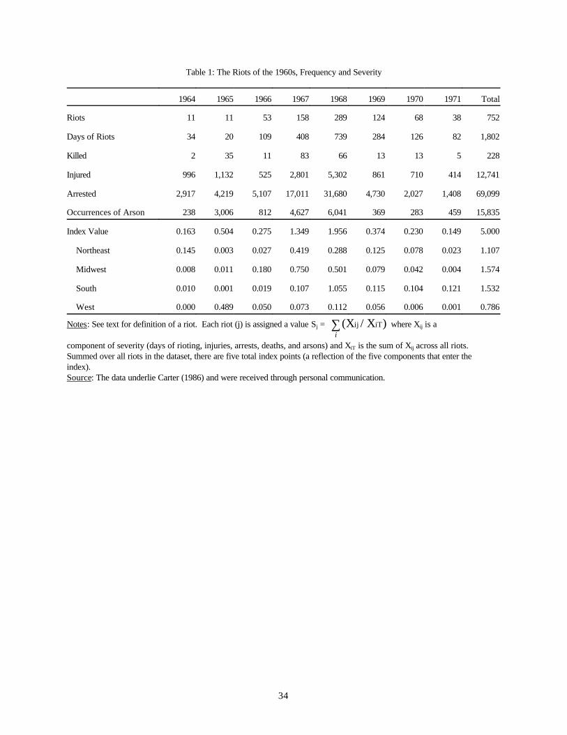
34

Table 1: The Riots of the 1960s, Frequency and Severity

1964 1965 1966 1967 1968 1969 1970 1971 Total

Riots 11 11 53 158 289 124 68 38 752

Days of Riots 34 20 109 408 739 284 126 82 1,802

Killed 2 35 11 83 66 13 13 5 228

Injured 996 1,132 525 2,801 5,302 861 710 414 12,741

Arrested 2,917 4,219 5,107 17,011 31,680 4,730 2,027 1,408 69,099

Occurrences of Arson 238 3,006 812 4,627 6,041 369 283 459 15,835

Index Value 0.163 0.504 0.275 1.349 1.956 0.374 0.230 0.149 5.000

Northeast 0.145 0.003 0.027 0.419 0.288 0.125 0.078 0.023 1.107

Midwest 0.008 0.011 0.180 0.750 0.501 0.079 0.042 0.004 1.574

South 0.010 0.001 0.019 0.107 1.055 0.115 0.104 0.121 1.532

West 0.000 0.489 0.050 0.073 0.112 0.056 0.006 0.001 0.786

Notes: See text for definition of a riot. Each riot (j) is assigned a value Sj = where Xij is a(X / Xij iTi

∑ )

component of severity (days of rioting, injuries, arrests, deaths, and arsons) and XiT is the sum of Xij across all riots. Summed over all riots in the dataset, there are five total index points (a reflection of the five components that enter theindex). Source: The data underlie Carter (1986) and were received through personal communication.

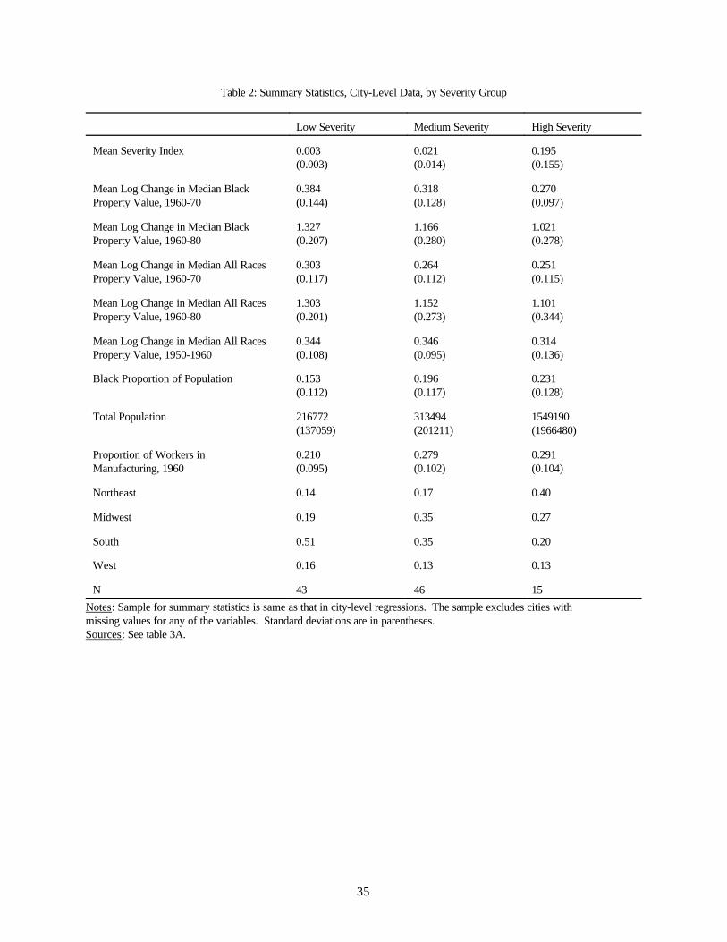
35

Table 2: Summary Statistics, City-Level Data, by Severity Group

Low Severity Medium Severity High Severity

Mean Severity Index 0.003(0.003)

0.021(0.014)

0.195(0.155)

Mean Log Change in Median BlackProperty Value, 1960-70

0.384(0.144)

0.318(0.128)

0.270(0.097)

Mean Log Change in Median BlackProperty Value, 1960-80

1.327(0.207)

1.166(0.280)

1.021(0.278)

Mean Log Change in Median All RacesProperty Value, 1960-70

0.303(0.117)

0.264(0.112)

0.251(0.115)

Mean Log Change in Median All RacesProperty Value, 1960-80

1.303(0.201)

1.152(0.273)

1.101(0.344)

Mean Log Change in Median All RacesProperty Value, 1950-1960

0.344(0.108)

0.346(0.095)

0.314(0.136)

Black Proportion of Population 0.153(0.112)

0.196(0.117)

0.231(0.128)

Total Population 216772(137059)

313494(201211)

1549190(1966480)

Proportion of Workers inManufacturing, 1960

0.210(0.095)

0.279(0.102)

0.291(0.104)

Northeast 0.14 0.17 0.40

Midwest 0.19 0.35 0.27

South 0.51 0.35 0.20

West 0.16 0.13 0.13

N 43 46 15

Notes: Sample for summary statistics is same as that in city-level regressions. The sample excludes cities withmissing values for any of the variables. Standard deviations are in parentheses.Sources: See table 3A.

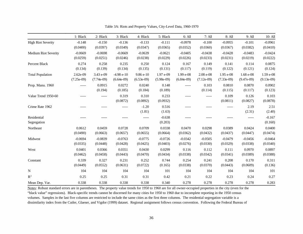
36

Table 3A: Riots and Property Values, City-Level Data, 1960-1970

1: Black 2: Black 3: Black 4: Black 5: Black 6: All 7: All 8: All 9: All 10: All

High Riot Severity -0.148(0.0400)

-0.150(0.0397)

-0.136(0.0349)

-0.133(0.0347)

-0.111(0.0365)

-0.0978(0.0352)

-0.100(0.0360)

-0.0955(0.0367)

-0.101(0.0382)

-0.0961(0.0410)

Medium Riot Severity -0.0669(0.0259)

-0.0698(0.0251)

-0.0669(0.0246)

-0.0639(0.0238)

-0.0621(0.0229)

-0.0405(0.0226)

-0.0438(0.0233)

-0.0428(0.0231)

-0.0483(0.0219)

-0.0424(0.0222)

Percent Black 0.274(0.134)

0.258(0.139)

0.235(0.134)

0.250(0.135)

0.124(0.131)

0.167(0.117)

0.149(0.119)

0.141(0.122)

0.114(0.121)

0.0875(0.124)

Total Population 2.62e-09(7.25e-09)

3.43 e-09(7.74e-09)

-4.98 e-10(6.64e-09)

9.86 e-10(6.53e-09)

1.97 e-09(5.98e-09)

1.99 e-08(6.84e-09)

2.08 e-08(7.12e-09)

1.95 e-08(7.33e-09)

1.68 e-08(9.47e-09)

1.59 e-08(9.13e-09)

Prop. Manu. 1960 ----- 0.0915(0.194)

0.0272(0.185)

0.0240(0.184)

0.148(0.189)

----- 0.103(0.114)

0.0810(0.115)

0.0870(0.117)

0.0902(0.123)

Value Trend 1950-60 ----- ----- 0.319(0.0872)

0.310(0.0892)

0.233(0.0932)

----- ----- 0.109(0.0811)

0.126(0.0827)

0.103(0.0878)

Crime Rate 1962 ----- ----- ----- -1.20(1.81)

0.516(1.63)

----- ----- ----- 2.19(2.31)

2.51(2.40)

ResidentialSegregation

----- ----- ----- ----- -0.638(0.203)

----- ----- ----- ----- -0.167(0.160)

Northeast 0.0612(0.0490)

0.0459(0.0663)

0.0728(0.0657)

0.0709(0.0655)

0.0338(0.0664)

0.0470(0.0362)

0.0298(0.0432)

0.0389(0.0437)

0.0424(0.0447)

0.0400(0.0474)

Midwest -0.0694(0.0335)

-0.0839(0.0448)

-0.0763(0.0428)

-0.0775(0.0425)

-0.0726(0.0403)

-0.0342(0.0276)

-0.0505(0.0330)

-0.0479(0.0329)

-0.0456(0.0338)

-0.0464(0.0340)

West 0.0401(0.0462)

0.0366(0.0458)

0.0351(0.0443)

0.0430(0.0470)

0.0299(0.0434)

0.116(0.0338)

0.112(0.0342)

0.111(0.0341)

0.0970(0.0389)

0.0897(0.0388)

Constant 0.339(0.0449)

0.327(0.0552)

0.231(0.0631)

0.252(0.0722)

0.744(0.165)

0.254(0.0338)

0.241(0.0370)

0.208(0.0443)

0.170(0.0609)

0.311(0.136)

N 104 104 104 104 101 104 104 104 104 101

R2 0.25 0.25 0.31 0.31 0.42 0.21 0.22 0.23 0.24 0.27

Mean Dep. Var. 0.338 0.338 0.338 0.338 0.340 0.278 0.278 0.278 0.278 0.283Notes: Robust standard errors are in parentheses. The property value trends for 1950 to 1960 are for all owner-occupied properties in the city (even for the“black value” regressions). Black-specific trends cannot be discerned for many cities for 1950 to 1960 due to incomplete reporting in the 1950 censusvolumes. Samples in the last five columns are restricted to include the same cities as the first three columns. The residential segregation variable is adissimilarity index from the Cutler, Glaeser, and Vigdor (1999) dataset. Regional assignment follows census convention. Following the Federal Bureau of

37

Investigation’s Uniform Crime Reports, the crime rate is the ratio of total crimes in 1962 (excluding larceny under $50) to total population in 1960;Montgomery, Alabama’s figure is based on 1961 crime data.Sources: Property values are from the published volumes of the federal censuses of population and housing. Manufacturing and population variables for 1960are based on census data and taken from issues of the U.S. Department of Commerce, County and City Data Book (tabulated in ICPSR 7735 and checkedagainst data compiled by Michael Haines). Riot severity measures are based on data underlying Carter (1986). The crime rate data for 1962 are tabulatedfrom the Federal Bureau of Investigation’s Uniform Crime Reports, table 41. The Cutler, Glaeser, and Vigdor (1999) segregation data are available atwww.nber.org.

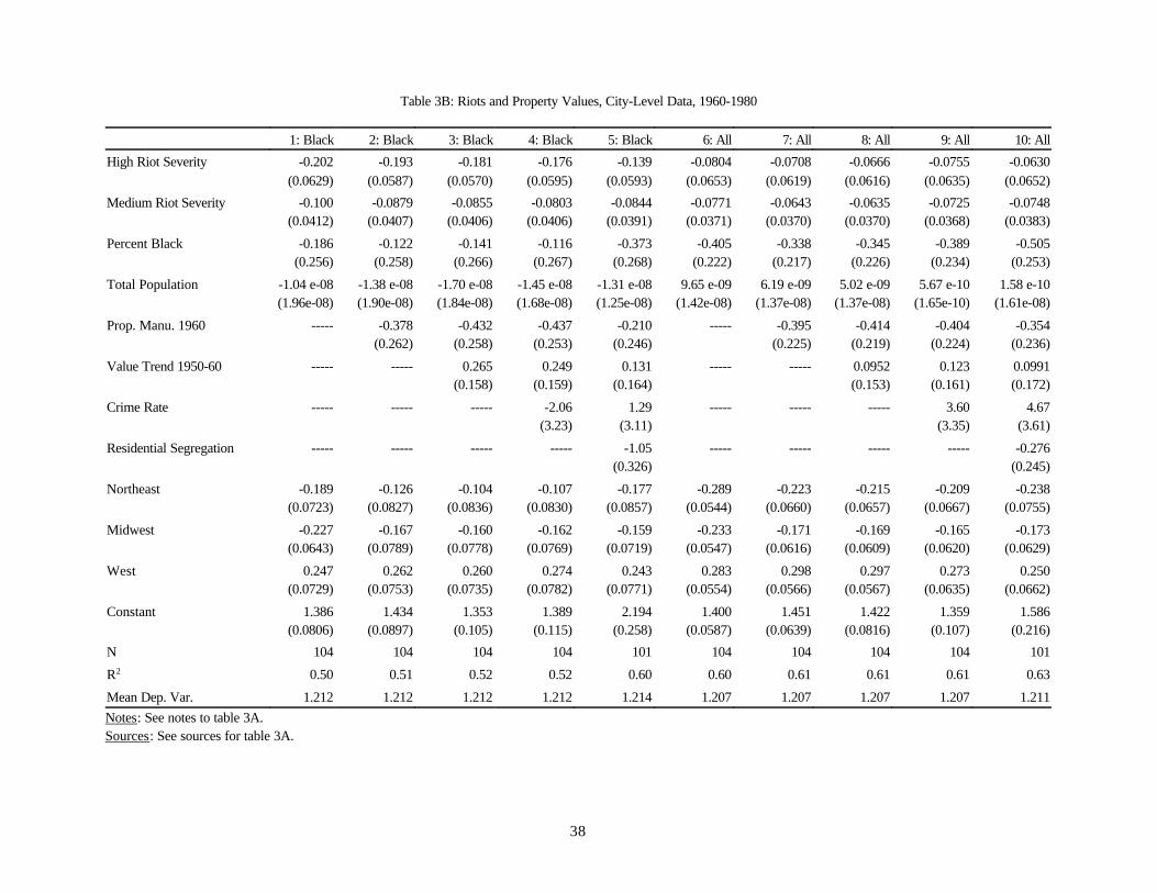
38

Table 3B: Riots and Property Values, City-Level Data, 1960-1980

1: Black 2: Black 3: Black 4: Black 5: Black 6: All 7: All 8: All 9: All 10: All

High Riot Severity -0.202(0.0629)

-0.193(0.0587)

-0.181(0.0570)

-0.176(0.0595)

-0.139(0.0593)

-0.0804(0.0653)

-0.0708(0.0619)

-0.0666(0.0616)

-0.0755(0.0635)

-0.0630(0.0652)

Medium Riot Severity -0.100(0.0412)

-0.0879(0.0407)

-0.0855(0.0406)

-0.0803(0.0406)

-0.0844(0.0391)

-0.0771(0.0371)

-0.0643(0.0370)

-0.0635(0.0370)

-0.0725(0.0368)

-0.0748(0.0383)

Percent Black -0.186(0.256)

-0.122(0.258)

-0.141(0.266)

-0.116(0.267)

-0.373(0.268)

-0.405(0.222)

-0.338(0.217)

-0.345(0.226)

-0.389(0.234)

-0.505(0.253)

Total Population -1.04 e-08(1.96e-08)

-1.38 e-08(1.90e-08)

-1.70 e-08(1.84e-08)

-1.45 e-08(1.68e-08)

-1.31 e-08(1.25e-08)

9.65 e-09(1.42e-08)

6.19 e-09(1.37e-08)

5.02 e-09(1.37e-08)

5.67 e-10(1.65e-10)

1.58 e-10(1.61e-08)

Prop. Manu. 1960 ----- -0.378(0.262)

-0.432(0.258)

-0.437(0.253)

-0.210(0.246)

----- -0.395(0.225)

-0.414(0.219)

-0.404(0.224)

-0.354(0.236)

Value Trend 1950-60 ----- ----- 0.265(0.158)

0.249(0.159)

0.131(0.164)

----- ----- 0.0952(0.153)

0.123(0.161)

0.0991(0.172)

Crime Rate ----- ----- ----- -2.06(3.23)

1.29(3.11)

----- ----- ----- 3.60(3.35)

4.67(3.61)

Residential Segregation ----- ----- ----- ----- -1.05(0.326)

----- ----- ----- ----- -0.276(0.245)

Northeast -0.189(0.0723)

-0.126(0.0827)

-0.104(0.0836)

-0.107(0.0830)

-0.177(0.0857)

-0.289(0.0544)

-0.223(0.0660)

-0.215(0.0657)

-0.209(0.0667)

-0.238(0.0755)

Midwest -0.227(0.0643)

-0.167(0.0789)

-0.160(0.0778)

-0.162(0.0769)

-0.159(0.0719)

-0.233(0.0547)

-0.171(0.0616)

-0.169(0.0609)

-0.165(0.0620)

-0.173(0.0629)

West 0.247(0.0729)

0.262(0.0753)

0.260(0.0735)

0.274(0.0782)

0.243(0.0771)

0.283(0.0554)

0.298(0.0566)

0.297(0.0567)

0.273(0.0635)

0.250(0.0662)

Constant 1.386(0.0806)

1.434(0.0897)

1.353(0.105)

1.389(0.115)

2.194(0.258)

1.400(0.0587)

1.451(0.0639)

1.422(0.0816)

1.359(0.107)

1.586(0.216)

N 104 104 104 104 101 104 104 104 104 101

R2 0.50 0.51 0.52 0.52 0.60 0.60 0.61 0.61 0.61 0.63

Mean Dep. Var. 1.212 1.212 1.212 1.212 1.214 1.207 1.207 1.207 1.207 1.211Notes: See notes to table 3A.Sources: See sources for table 3A.

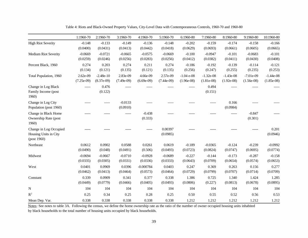
39

Table 4: Riots and Black-Owned Property Values, City-Level Data with Contemporaneous Controls, 1960-70 and 1960-80

1:1960-70 2:1960-70 3:1960-70 4:1960-70 5:1960-70 6:1960-80 7:1960-80 8:1960-80 9:1960-80 10:1960-80

High Riot Severity -0.148(0.0400)

-0.133(0.0431)

-0.149(0.0413)

-0.136(0.0442)

-0.148(0.0418)

-0.202(0.0629)

-0.159(0.0693)

-0.174(0.0661)

-0.158(0.0605)

-0.166(0.0665)

Medium Riot Severity -0.0669(0.0259)

-0.0721(0.0246)

-0.0665(0.0256)

-0.0575(0.0283)

-0.0669(0.0256)

-0.100(0.0412)

-0.0947(0.0382)

-0.101(0.0411)

-0.0683(0.0430)

-0.101(0.0408)

Percent Black, 1960 0.274(0.134)

0.203(0.121)

0.274(0.135)

0.211(0.121)

0.274(0.135)

-0.186(0.256)

-0.192(0.247)

-0.139(0.255)

-0.114(0.235)

-0.121(0.253)

Total Population, 1960 2.62e-09(7.25e-09)

-2.48e-10(8.37e-09)

2.83e-09(7.49e-09)

4.66e-09(6.69e-09)

2.57e-09(7.44e-09)

-1.04 e-08(1.96e-08)

-1.32e-08(1.81e-08)

-1.43e-08(1.92e-08)

-7.01e-09(1.56e-08)

-1.44e-08(1.85e-08)

Change in Log BlackFamily Income (post1960)

----- 0.476(0.122)

----- ----- ----- ----- 0.494(0.151)

----- ----- -----

Change in Log CityPopulation (post 1960)

----- ----- -0.0133(0.0910)

----- ----- ----- ----- 0.166(0.0984)

----- -----

Change in Black HomeOwnership Rate (post1960)

----- ----- ----- -0.438(0.333)

----- ----- ----- ----- -0.847(0.301)

-----

Change in Log OccupiedHousing Units in City(post 1960)

----- ----- ----- ----- 0.00397(0.0985)

----- ----- ----- ----- 0.201(0.0946)

Northeast 0.0612(0.0490)

0.0902(0.048)

0.0588(0.0491)

0.0261(0.506)

0.0619(0.0493)

-0.189(0.0723)

-0.0365(0.0824)

-0.124(0.0747)

-0.239(0.0695)

-0.0992(0.0774)

Midwest -0.0694(0.0335)

-0.0667(0.0305)

-0.0710(0.0331)

-0.0928(0.0336)

-0.0689(0.0333)

-0.227(0.0643)

-0.144(0.0709)

-0.173(0.0654)

-0.287(0.0574)

-0.158(0.0653)

West 0.0401(0.0462)

0.0969(0.0413)

0.0396(0.0464)

-0.000784(0.0573)

0.0403(0.0464)

0.247(0.0729)

0.369(0.0799)

0.263(0.0707)

0.156(0.0714)

0.277(0.0709)

Constant 0.339(0.0449)

0.0909(0.0779)

0.341(0.0466)

0.377(0.0405)

0.338(0.0493)

1.386(0.0806)

0.725(0.227)

1.340(0.0813)

1.424(0.0678)

1.285(0.0895)

N 104 104 104 104 104 104 104 104 104 104

R2 0.25 0.34 0.25 0.28 0.25 0.50 0.55 0.52 0.56 0.53

Mean Dep. Var. 0.338 0.338 0.338 0.338 0.338 1.212 1.212 1.212 1.212 1.212Notes: See notes to table 3A. Following the census, we define the home ownership rate as the ratio of the number of owner occupied housing units inhabitedby black households to the total number of housing units occupied by black households.

40

Sources: See sources for table 3A.

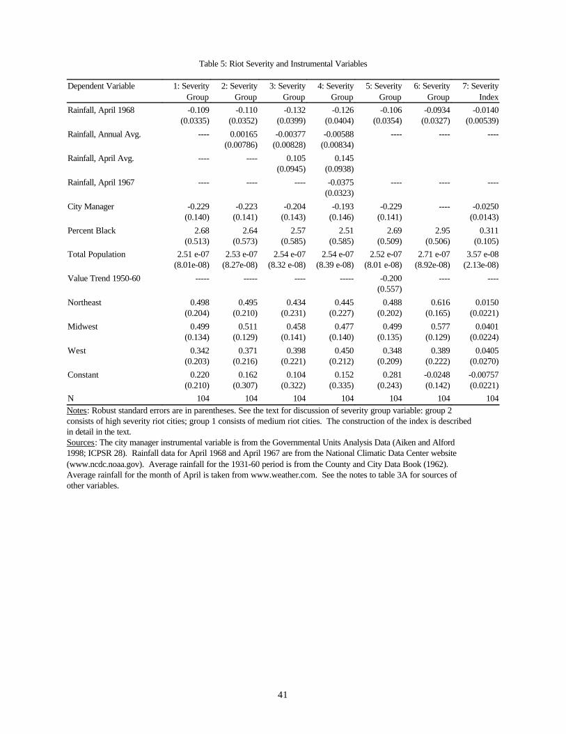
41

Table 5: Riot Severity and Instrumental Variables

Dependent Variable 1: SeverityGroup

2: SeverityGroup

3: SeverityGroup

4: SeverityGroup

5: SeverityGroup

6: SeverityGroup

7: Severity Index

Rainfall, April 1968 -0.109(0.0335)

-0.110(0.0352)

-0.132(0.0399)

-0.126(0.0404)

-0.106(0.0354)

-0.0934(0.0327)

-0.0140(0.00539)

Rainfall, Annual Avg. ---- 0.00165(0.00786)

-0.00377(0.00828)

-0.00588(0.00834)

---- ---- ----

Rainfall, April Avg. ---- ---- 0.105(0.0945)

0.145(0.0938)

Rainfall, April 1967 ---- ---- ---- -0.0375(0.0323)

---- ---- ----

City Manager -0.229(0.140)

-0.223(0.141)

-0.204(0.143)

-0.193(0.146)

-0.229(0.141)

---- -0.0250(0.0143)

Percent Black 2.68(0.513)

2.64(0.573)

2.57(0.585)

2.51(0.585)

2.69(0.509)

2.95(0.506)

0.311(0.105)

Total Population 2.51 e-07(8.01e-08)

2.53 e-07(8.27e-08)

2.54 e-07(8.32 e-08)

2.54 e-07(8.39 e-08)

2.52 e-07(8.01 e-08)

2.71 e-07(8.92e-08)

3.57 e-08(2.13e-08)

Value Trend 1950-60 ----- ----- ---- ----- -0.200(0.557)

---- ----

Northeast 0.498(0.204)

0.495(0.210)

0.434(0.231)

0.445(0.227)

0.488(0.202)

0.616(0.165)

0.0150(0.0221)

Midwest 0.499(0.134)

0.511(0.129)

0.458(0.141)

0.477(0.140)

0.499(0.135)

0.577(0.129)

0.0401(0.0224)

West 0.342(0.203)

0.371(0.216)

0.398(0.221)

0.450(0.212)

0.348(0.209)

0.389(0.222)

0.0405(0.0270)

Constant 0.220(0.210)

0.162(0.307)

0.104(0.322)

0.152(0.335)

0.281(0.243)

-0.0248(0.142)

-0.00757(0.0221)

N 104 104 104 104 104 104 104Notes: Robust standard errors are in parentheses. See the text for discussion of severity group variable: group 2consists of high severity riot cities; group 1 consists of medium riot cities. The construction of the index is describedin detail in the text. Sources: The city manager instrumental variable is from the Governmental Units Analysis Data (Aiken and Alford1998; ICPSR 28). Rainfall data for April 1968 and April 1967 are from the National Climatic Data Center website(www.ncdc.noaa.gov). Average rainfall for the 1931-60 period is from the County and City Data Book (1962). Average rainfall for the month of April is taken from www.weather.com. See the notes to table 3A for sources ofother variables.

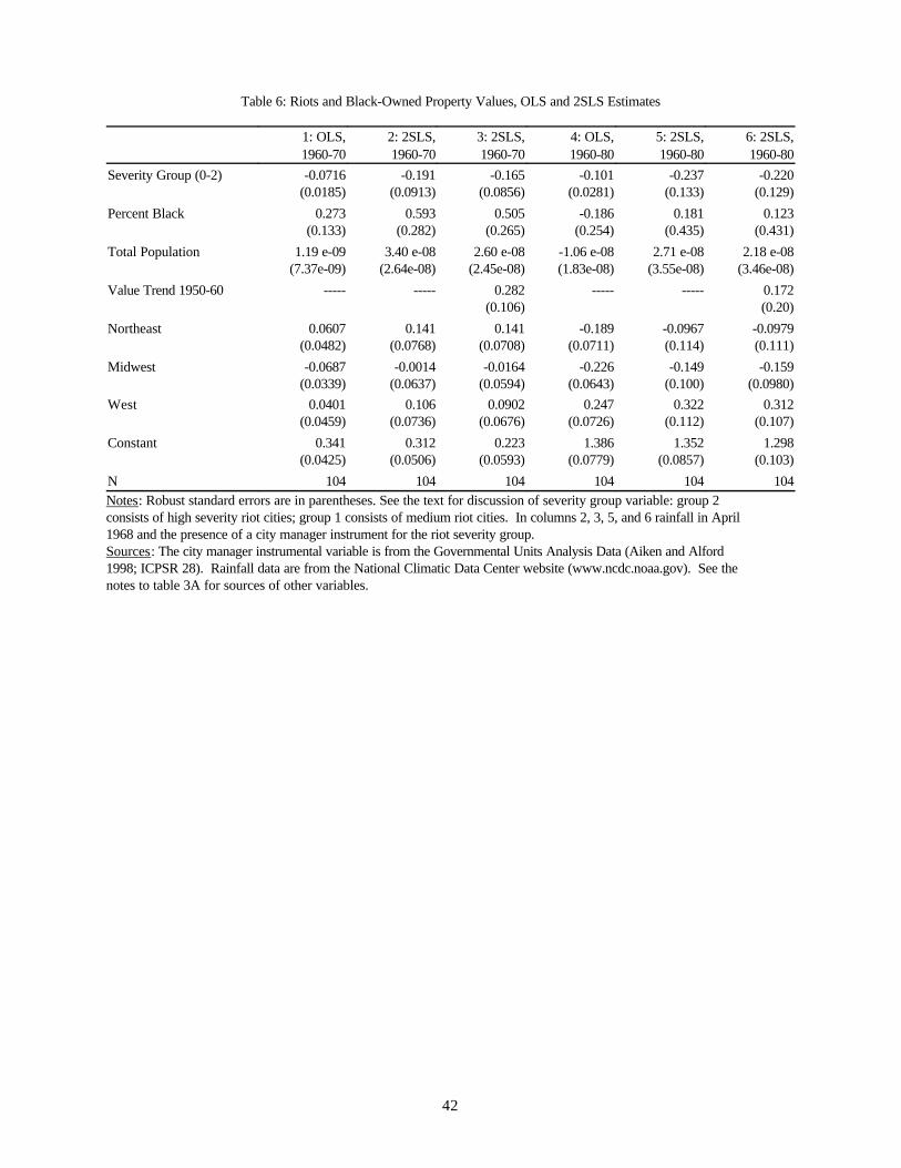
42

Table 6: Riots and Black-Owned Property Values, OLS and 2SLS Estimates

1: OLS,1960-70

2: 2SLS,1960-70

3: 2SLS,1960-70

4: OLS,1960-80

5: 2SLS,1960-80

6: 2SLS,1960-80

Severity Group (0-2) -0.0716(0.0185)

-0.191(0.0913)

-0.165(0.0856)

-0.101(0.0281)

-0.237(0.133)

-0.220(0.129)

Percent Black 0.273(0.133)

0.593(0.282)

0.505(0.265)

-0.186(0.254)

0.181(0.435)

0.123(0.431)

Total Population 1.19 e-09(7.37e-09)

3.40 e-08(2.64e-08)

2.60 e-08(2.45e-08)

-1.06 e-08(1.83e-08)

2.71 e-08(3.55e-08)

2.18 e-08(3.46e-08)

Value Trend 1950-60 ----- ----- 0.282(0.106)

----- ----- 0.172(0.20)

Northeast 0.0607(0.0482)

0.141(0.0768)

0.141(0.0708)

-0.189(0.0711)

-0.0967(0.114)

-0.0979(0.111)

Midwest -0.0687(0.0339)

-0.0014(0.0637)

-0.0164(0.0594)

-0.226(0.0643)

-0.149(0.100)

-0.159(0.0980)

West 0.0401(0.0459)

0.106(0.0736)

0.0902(0.0676)

0.247(0.0726)

0.322(0.112)

0.312(0.107)

Constant 0.341(0.0425)

0.312(0.0506)

0.223(0.0593)

1.386(0.0779)

1.352(0.0857)

1.298(0.103)

N 104 104 104 104 104 104Notes: Robust standard errors are in parentheses. See the text for discussion of severity group variable: group 2consists of high severity riot cities; group 1 consists of medium riot cities. In columns 2, 3, 5, and 6 rainfall in April1968 and the presence of a city manager instrument for the riot severity group.Sources: The city manager instrumental variable is from the Governmental Units Analysis Data (Aiken and Alford1998; ICPSR 28). Rainfall data are from the National Climatic Data Center website (www.ncdc.noaa.gov). See thenotes to table 3A for sources of other variables.

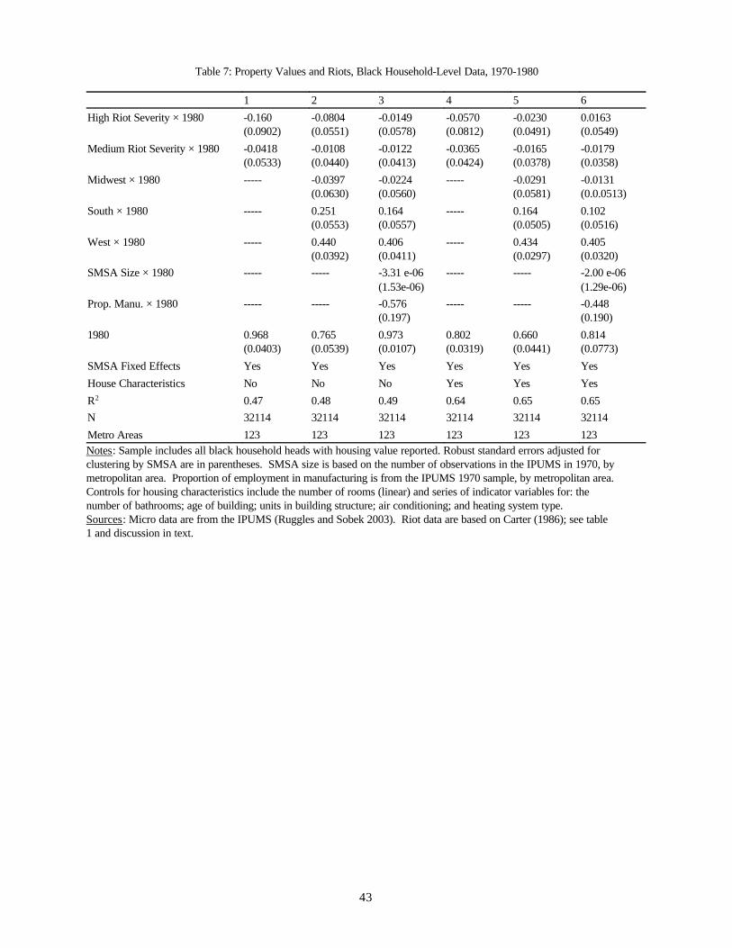
43

Table 7: Property Values and Riots, Black Household-Level Data, 1970-1980

1 2 3 4 5 6

High Riot Severity × 1980 -0.160(0.0902)

-0.0804(0.0551)

-0.0149(0.0578)

-0.0570(0.0812)

-0.0230(0.0491)

0.0163(0.0549)

Medium Riot Severity × 1980 -0.0418(0.0533)

-0.0108(0.0440)

-0.0122(0.0413)

-0.0365(0.0424)

-0.0165(0.0378)

-0.0179(0.0358)

Midwest × 1980 ----- -0.0397(0.0630)

-0.0224(0.0560)

----- -0.0291(0.0581)

-0.0131(0.0.0513)

South × 1980 ----- 0.251(0.0553)

0.164(0.0557)

----- 0.164(0.0505)

0.102(0.0516)

West × 1980 ----- 0.440(0.0392)

0.406(0.0411)

----- 0.434(0.0297)

0.405(0.0320)

SMSA Size × 1980 ----- ----- -3.31 e-06(1.53e-06)

----- ----- -2.00 e-06(1.29e-06)

Prop. Manu. × 1980 ----- ----- -0.576(0.197)

----- ----- -0.448(0.190)

1980 0.968(0.0403)

0.765(0.0539)

0.973(0.0107)

0.802(0.0319)

0.660(0.0441)

0.814(0.0773)

SMSA Fixed Effects Yes Yes Yes Yes Yes Yes

House Characteristics No No No Yes Yes Yes

R2 0.47 0.48 0.49 0.64 0.65 0.65N 32114 32114 32114 32114 32114 32114

Metro Areas 123 123 123 123 123 123Notes: Sample includes all black household heads with housing value reported. Robust standard errors adjusted forclustering by SMSA are in parentheses. SMSA size is based on the number of observations in the IPUMS in 1970, bymetropolitan area. Proportion of employment in manufacturing is from the IPUMS 1970 sample, by metropolitan area. Controls for housing characteristics include the number of rooms (linear) and series of indicator variables for: thenumber of bathrooms; age of building; units in building structure; air conditioning; and heating system type.Sources: Micro data are from the IPUMS (Ruggles and Sobek 2003). Riot data are based on Carter (1986); see table1 and discussion in text.

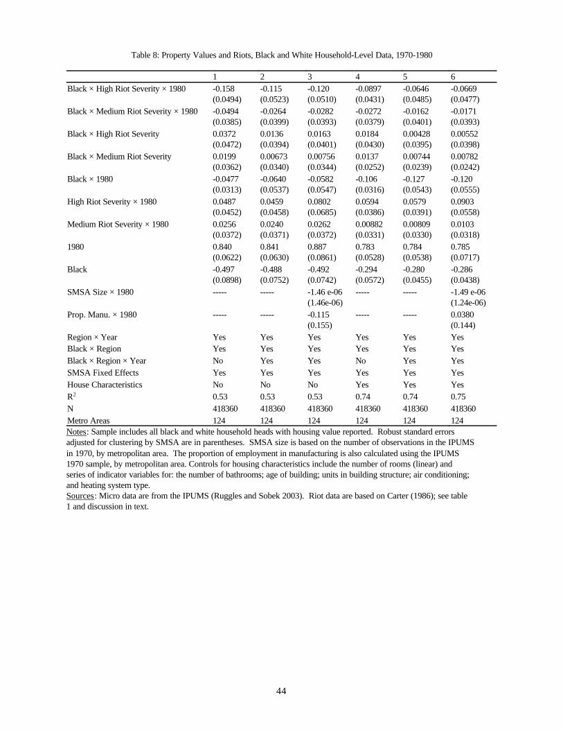
44

Table 8: Property Values and Riots, Black and White Household-Level Data, 1970-1980

1 2 3 4 5 6Black × High Riot Severity × 1980 -0.158

(0.0494)-0.115(0.0523)

-0.120(0.0510)

-0.0897(0.0431)

-0.0646(0.0485)

-0.0669(0.0477)

Black × Medium Riot Severity × 1980 -0.0494(0.0385)

-0.0264(0.0399)

-0.0282(0.0393)

-0.0272(0.0379)

-0.0162(0.0401)

-0.0171(0.0393)

Black × High Riot Severity 0.0372(0.0472)

0.0136(0.0394)

0.0163(0.0401)

0.0184(0.0430)

0.00428(0.0395)

0.00552(0.0398)

Black × Medium Riot Severity 0.0199(0.0362)

0.00673(0.0340)

0.00756(0.0344)

0.0137(0.0252)

0.00744(0.0239)

0.00782(0.0242)

Black × 1980 -0.0477(0.0313)

-0.0640(0.0537)

-0.0582(0.0547)

-0.106(0.0316)

-0.127(0.0543)

-0.120(0.0555)

High Riot Severity × 1980 0.0487(0.0452)

0.0459(0.0458)

0.0802(0.0685)

0.0594(0.0386)

0.0579(0.0391)

0.0903(0.0558)

Medium Riot Severity × 1980 0.0256(0.0372)

0.0240(0.0371)

0.0262(0.0372)

0.00882(0.0331)

0.00809(0.0330)

0.0103(0.0318)

1980 0.840(0.0622)

0.841(0.0630)

0.887(0.0861)

0.783(0.0528)

0.784(0.0538)

0.785(0.0717)

Black -0.497(0.0898)

-0.488(0.0752)

-0.492(0.0742)

-0.294(0.0572)

-0.280(0.0455)

-0.286(0.0438)

SMSA Size × 1980 ----- ----- -1.46 e-06(1.46e-06)

----- ----- -1.49 e-06(1.24e-06)

Prop. Manu. × 1980 ----- ----- -0.115(0.155)

----- ----- 0.0380(0.144)

Region × Year Yes Yes Yes Yes Yes YesBlack × Region Yes Yes Yes Yes Yes YesBlack × Region × Year No Yes Yes No Yes YesSMSA Fixed Effects Yes Yes Yes Yes Yes YesHouse Characteristics No No No Yes Yes YesR2 0.53 0.53 0.53 0.74 0.74 0.75N 418360 418360 418360 418360 418360 418360Metro Areas 124 124 124 124 124 124Notes: Sample includes all black and white household heads with housing value reported. Robust standard errorsadjusted for clustering by SMSA are in parentheses. SMSA size is based on the number of observations in the IPUMSin 1970, by metropolitan area. The proportion of employment in manufacturing is also calculated using the IPUMS1970 sample, by metropolitan area. Controls for housing characteristics include the number of rooms (linear) andseries of indicator variables for: the number of bathrooms; age of building; units in building structure; air conditioning;and heating system type.Sources: Micro data are from the IPUMS (Ruggles and Sobek 2003). Riot data are based on Carter (1986); see table1 and discussion in text.

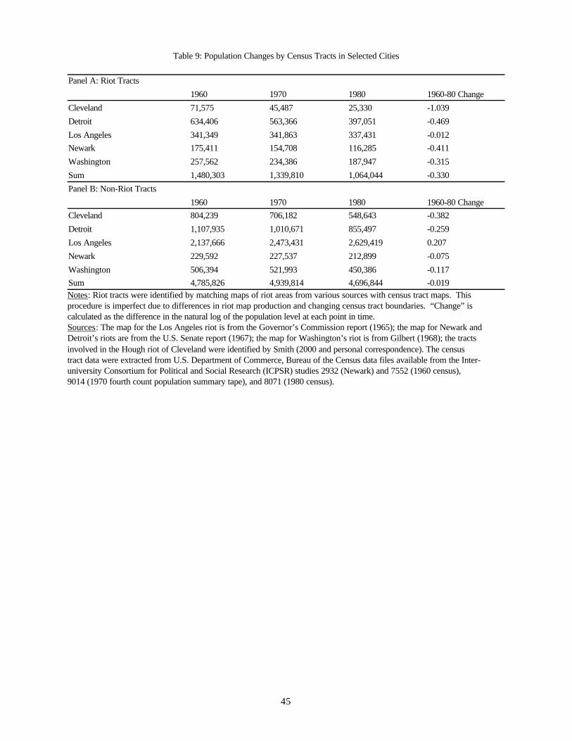
45

Table 9: Population Changes by Census Tracts in Selected Cities

Panel A: Riot Tracts

1960 1970 1980 1960-80 Change

Cleveland 71,575 45,487 25,330 -1.039

Detroit 634,406 563,366 397,051 -0.469

Los Angeles 341,349 341,863 337,431 -0.012Newark 175,411 154,708 116,285 -0.411

Washington 257,562 234,386 187,947 -0.315

Sum 1,480,303 1,339,810 1,064,044 -0.330

Panel B: Non-Riot Tracts

1960 1970 1980 1960-80 ChangeCleveland 804,239 706,182 548,643 -0.382

Detroit 1,107,935 1,010,671 855,497 -0.259

Los Angeles 2,137,666 2,473,431 2,629,419 0.207

Newark 229,592 227,537 212,899 -0.075

Washington 506,394 521,993 450,386 -0.117Sum 4,785,826 4,939,814 4,696,844 -0.019Notes: Riot tracts were identified by matching maps of riot areas from various sources with census tract maps. Thisprocedure is imperfect due to differences in riot map production and changing census tract boundaries. “Change” iscalculated as the difference in the natural log of the population level at each point in time. Sources: The map for the Los Angeles riot is from the Governor’s Commission report (1965); the map for Newark andDetroit’s riots are from the U.S. Senate report (1967); the map for Washington’s riot is from Gilbert (1968); the tractsinvolved in the Hough riot of Cleveland were identified by Smith (2000 and personal correspondence). The censustract data were extracted from U.S. Department of Commerce, Bureau of the Census data files available from the Inter-university Consortium for Political and Social Research (ICPSR) studies 2932 (Newark) and 7552 (1960 census),9014 (1970 fourth count population summary tape), and 8071 (1980 census).

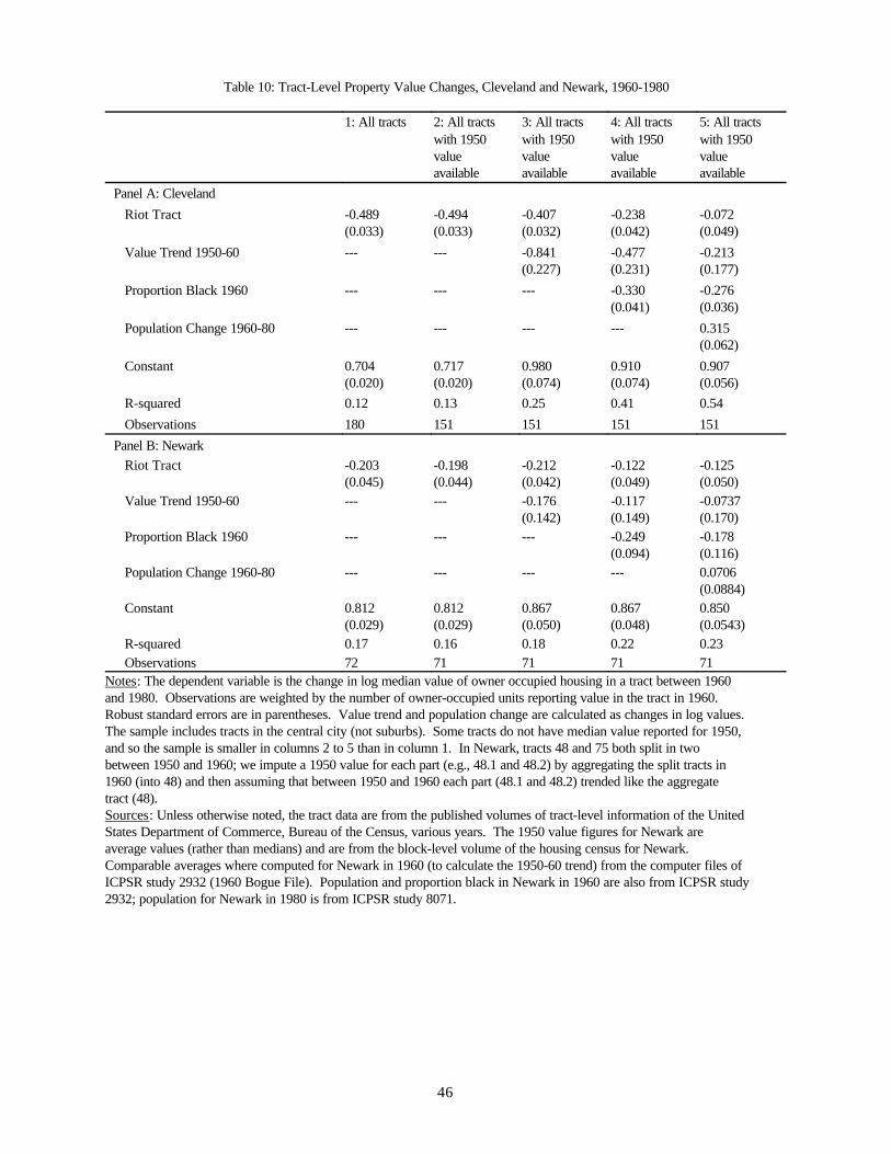
46

Table 10: Tract-Level Property Value Changes, Cleveland and Newark, 1960-1980

1: All tracts 2: All tractswith 1950valueavailable

3: All tractswith 1950valueavailable

4: All tractswith 1950valueavailable

5: All tractswith 1950valueavailable

Panel A: Cleveland

Riot Tract -0.489(0.033)

-0.494(0.033)

-0.407(0.032)

-0.238(0.042)

-0.072(0.049)

Value Trend 1950-60 --- --- -0.841(0.227)

-0.477(0.231)

-0.213(0.177)

Proportion Black 1960 --- --- --- -0.330(0.041)

-0.276(0.036)

Population Change 1960-80 --- --- --- --- 0.315(0.062)

Constant 0.704(0.020)

0.717(0.020)

0.980(0.074)

0.910(0.074)

0.907(0.056)

R-squared 0.12 0.13 0.25 0.41 0.54

Observations 180 151 151 151 151

Panel B: Newark Riot Tract -0.203

(0.045)-0.198(0.044)

-0.212(0.042)

-0.122(0.049)

-0.125(0.050)

Value Trend 1950-60 --- --- -0.176(0.142)

-0.117(0.149)

-0.0737(0.170)

Proportion Black 1960 --- --- --- -0.249(0.094)

-0.178(0.116)

Population Change 1960-80 --- --- --- --- 0.0706(0.0884)

Constant 0.812(0.029)

0.812(0.029)

0.867(0.050)

0.867(0.048)

0.850(0.0543)

R-squared 0.17 0.16 0.18 0.22 0.23 Observations 72 71 71 71 71

Notes: The dependent variable is the change in log median value of owner occupied housing in a tract between 1960and 1980. Observations are weighted by the number of owner-occupied units reporting value in the tract in 1960. Robust standard errors are in parentheses. Value trend and population change are calculated as changes in log values. The sample includes tracts in the central city (not suburbs). Some tracts do not have median value reported for 1950,and so the sample is smaller in columns 2 to 5 than in column 1. In Newark, tracts 48 and 75 both split in twobetween 1950 and 1960; we impute a 1950 value for each part (e.g., 48.1 and 48.2) by aggregating the split tracts in1960 (into 48) and then assuming that between 1950 and 1960 each part (48.1 and 48.2) trended like the aggregatetract (48).Sources: Unless otherwise noted, the tract data are from the published volumes of tract-level information of the UnitedStates Department of Commerce, Bureau of the Census, various years. The 1950 value figures for Newark areaverage values (rather than medians) and are from the block-level volume of the housing census for Newark. Comparable averages where computed for Newark in 1960 (to calculate the 1950-60 trend) from the computer files ofICPSR study 2932 (1960 Bogue File). Population and proportion black in Newark in 1960 are also from ICPSR study2932; population for Newark in 1980 is from ICPSR study 8071.

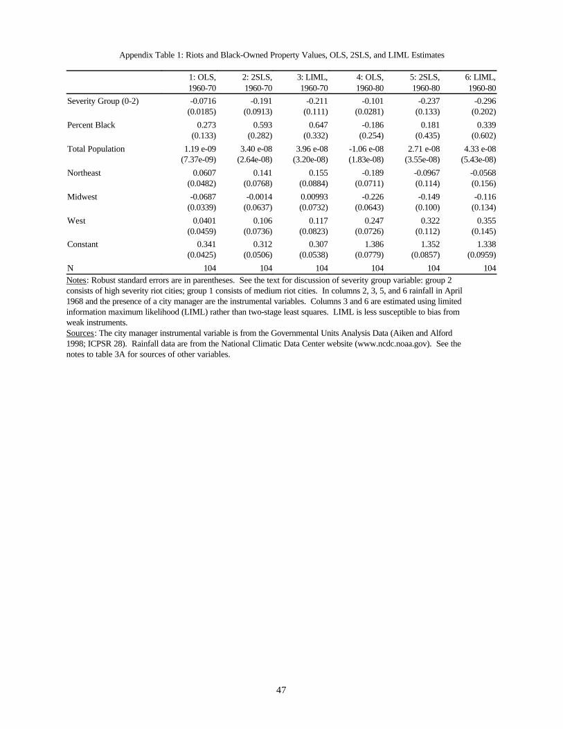
47

Appendix Table 1: Riots and Black-Owned Property Values, OLS, 2SLS, and LIML Estimates

1: OLS,1960-70

2: 2SLS,1960-70

3: LIML,1960-70

4: OLS,1960-80

5: 2SLS,1960-80

6: LIML,1960-80

Severity Group (0-2) -0.0716(0.0185)

-0.191(0.0913)

-0.211(0.111)

-0.101(0.0281)

-0.237(0.133)

-0.296(0.202)

Percent Black 0.273(0.133)

0.593(0.282)

0.647(0.332)

-0.186(0.254)

0.181(0.435)

0.339(0.602)

Total Population 1.19 e-09(7.37e-09)

3.40 e-08(2.64e-08)

3.96 e-08(3.20e-08)

-1.06 e-08(1.83e-08)

2.71 e-08(3.55e-08)

4.33 e-08(5.43e-08)

Northeast 0.0607(0.0482)

0.141(0.0768)

0.155(0.0884)

-0.189(0.0711)

-0.0967(0.114)

-0.0568(0.156)

Midwest -0.0687(0.0339)

-0.0014(0.0637)

0.00993(0.0732)

-0.226(0.0643)

-0.149(0.100)

-0.116(0.134)

West 0.0401(0.0459)

0.106(0.0736)

0.117(0.0823)

0.247(0.0726)

0.322(0.112)

0.355(0.145)

Constant 0.341(0.0425)

0.312(0.0506)

0.307(0.0538)

1.386(0.0779)

1.352(0.0857)

1.338(0.0959)

N 104 104 104 104 104 104Notes: Robust standard errors are in parentheses. See the text for discussion of severity group variable: group 2consists of high severity riot cities; group 1 consists of medium riot cities. In columns 2, 3, 5, and 6 rainfall in April1968 and the presence of a city manager are the instrumental variables. Columns 3 and 6 are estimated using limitedinformation maximum likelihood (LIML) rather than two-stage least squares. LIML is less susceptible to bias fromweak instruments.Sources: The city manager instrumental variable is from the Governmental Units Analysis Data (Aiken and Alford1998; ICPSR 28). Rainfall data are from the National Climatic Data Center website (www.ncdc.noaa.gov). See thenotes to table 3A for sources of other variables.