Embed Size (px)
Citation preview
FACULDADE DE ECONOMIA
PROGRAMA DE PÓS-GRADUAÇÃO EM ECONOMIA APLICADA
THE EARNING LOSSES AFTER
MIGRATION IN BRAZIL
Ricardo da Silva Freguglia
Naercio Aquino Menezes Filho
TD. 012/2008
Programa de Pos-Graduação em Economia Aplicada -
FE/UFJF
Juiz de Fora
2008
2
THE EARNING LOSSES AFTER MIGRATION IN BRAZIL
Ricardo da Silva Freguglia
Federal University of Juiz de Fora – Brazil and University of São Paulo – Brazil
Naercio Aquino Menezes-Filho
University of São Paulo – Brazil and IBMEC São Paulo – Brazil
Abstract
This paper evaluates the migration returns of workers in Brazil, focusing the assimilation process of
workers in São Paulo state. Specifically, its goal is to estimate the relative wage with the control for the
individual fixed effects, avoiding the bias from the positive selection of in-migrants. The results attest the
evidence of selection bias in the relative wages estimated by OLS, since the coefficients of the fixed
effects regression are lower (and with a negative signal) than the (positive) OLS coefficients. There are
wage losses to the migrants in São Paulo, who are not aware of the high cost of living. Another important
result is that the wage growth of migrants has been increasing slowly according to the local human capital
they have acquired since their migration. It is important to highlight that some particular groups have a
successful migration. Migrants with high levels of education have returns 7 percent higher than non-
migrants. Other groups, which also have gains after migration, are workers from agriculture and trade,
from Northeast region and from farming and scientific occupations. Finally, the out-migration gains are
positive and significant, even after the inclusion of the fixed effect control. As a result, the cost of living
is also an important factor to be considered in the São Paulo out-migration event.
Key words: 1. Migration; 2. Wages; 3. Self-selection; 4. Assimilation; 5. Fixed-effects; 6. Brazil.
JEL Classification: J24, J31, J61, F22
1. Introduction
The effects of migration on wages in the host region depend mostly on the way the abilities
distribution of migrants can be compared to the abilities distribution of non-migrant population. A
stylized fact of this literature is that migrants are not a random sample from the source region. In this
sense, using panel data of the RAIS-Migra from 1995 and 2002, the aim of this paper is to estimate the
impacts of migration and assimilation on wage differentials.
Specifically, the data allow tracking workers in the labor market among different Brazilian states
along the time, with information about wages before and after migration. As a result, we can use the fixed
3
effects method in order to control the self-selection bias. First, we analyses the effects of migration on
wages. Second, we examine the economic adjustment of migrants, estimating the effect of assimilation on
wages. Then, the main contribution of this study is to evaluate the wage differentials of migrants in the
host region after the control of non-observable characteristics.
In case of migration in Brazil, São Paulo is the state that absorbs the most part of migrants.
Additionally, the flow of workers and the wage differentials among São Paulo and the other Brazilian
states as well are important. In this sense, the analysis will focus on the labor market of this state.
The most important results attest the presence of omitted bias in OLS regressions as a
consequence of migrants’ self-selection. Seemingly, migrants have wage gains relative to non-migrants in
the OLS regressions. However, this wage advantage expires when we include the control of non-
observable abilities. The negative coefficient obtained from fixed effects wage regressions shows the
wage losses to the worker after migration to São Paulo. Most part of these losses are a result of the higher
cost of living in such state. In the assimilation analysis, the evidences show that the period of residence in
São Paulo is an important variable to determine the migrant earnings after the inclusion of individual
fixed effects. There is a wage convergence after 1.4 years, but the returns growth occurs at decreasing
rates in 3 years at most. At least, the gains from out-migration are positive, even after the inclusion of
fixed effects. This can be understood since the cost of living in São Paulo is an important factor in the
out-migration event.
This paper is organized as follows. The next section presents the database used and the summary
statistics. The econometric model of the migration impact on wages is presented in section 3. Following,
the results of return estimated considering observable and non-observable characteristics, and the
assimilation process are presented in section 4. Finally, we present the concluding remarks in section 5.
2. Data source and summary statistics
The database used in this paper is the RAIS-Migra, a panel data from the Labor Ministry of Brazil.
Its main characteristic is to track the same worker in the formal labor market with information about their
wages before and after the migration. As we have a large number of individuals – about 24 million
workers in the formal sector a year –, we built a one percent random sample from the total. The dataset
was drawn to follow the professional route of workers who were in the São Paulo state at least in one of
the years between 1995 and 2002. First, we used a balanced panel, which have 172.536 observations and
the same number of 21,567 individuals by year (see table 1). The migrants are almost 2% from the total of
personnel. Second, we considered the unbalanced panel, with 262,751 observations. The number of
individuals is not the same over years, because of workers were not always employed in the formal labor
market in the period. As a result, the migrant percentage in the unbalanced panel is almost 3%, larger than
in the balanced panel.
<TABLE 1 ABOUT HERE>
The empirical analysis is conducted to workers from 14 to 65 years old and with non-zero
earnings.1 The migration variable turns to 1 when the worker moves to São Paulo and continues
computing this value while he stays in this state. It turns to 0 when there is not migration or when the
worker leaves São Paulo. Another important variable is the years since migration, which computes the
number of years the worker stays in São Paulo after migration and turns to zero when the person is a
settler. The other variables used in the analysis are: age, tenure, gender, education, industry, occupation,
and the year dummies.
Another important group to be analyzed are the workers that egress from São Paulo. The out-
migration variable is similarly defined to the in-migration, assuming a value equal to 1 when the
individual exit from São Paulo and while staying in another state. A particular group of out-migrants are
1 The earnings are obtained from RAIS-Migra in nominal minimum wages. They were converted to Reais, deflated by the
IPCA – a Brazilian price index for consume –, and after by the ICV – a cost of living index – computed by Azzoni et al.
(2003).
4
the returning migrants, i.e., workers who moved to São Paulo in a specific year and came back to their
source state after some years. The variable of return migration is equal to 1 when this kind of worker
mobility occurs, and equal to 0 otherwise.
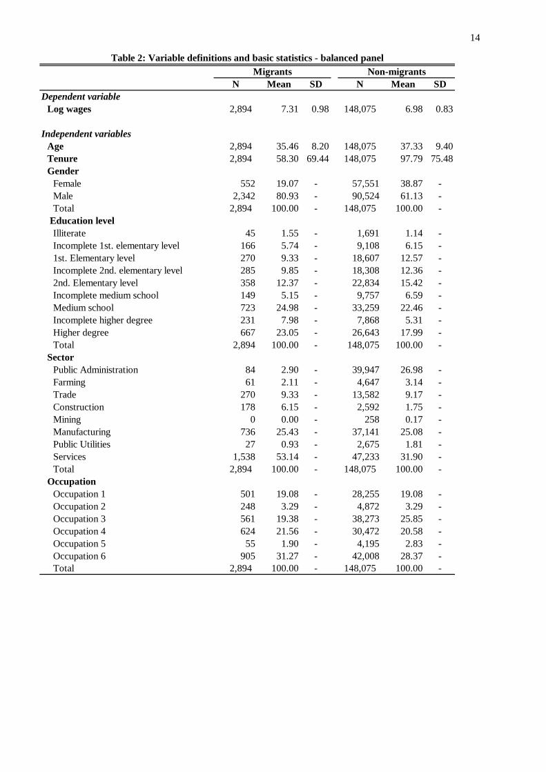
Considering the balanced panel, as we can see in table 2, the average profile of the migrant is 35
years old, male (85%), with tenure of about 5 years, high school (25%), from the service sector (53%),
and from blue-collar occupations (31%). The number of migrants in this panel is 2,894, approximately
2% of the workers as a whole. They are more educated, are mainly males, and are concentrated in the
service sector and in the blue-collar occupations than non-migrants. On the other hand, they have less
tenure, and the age is slightly lower.
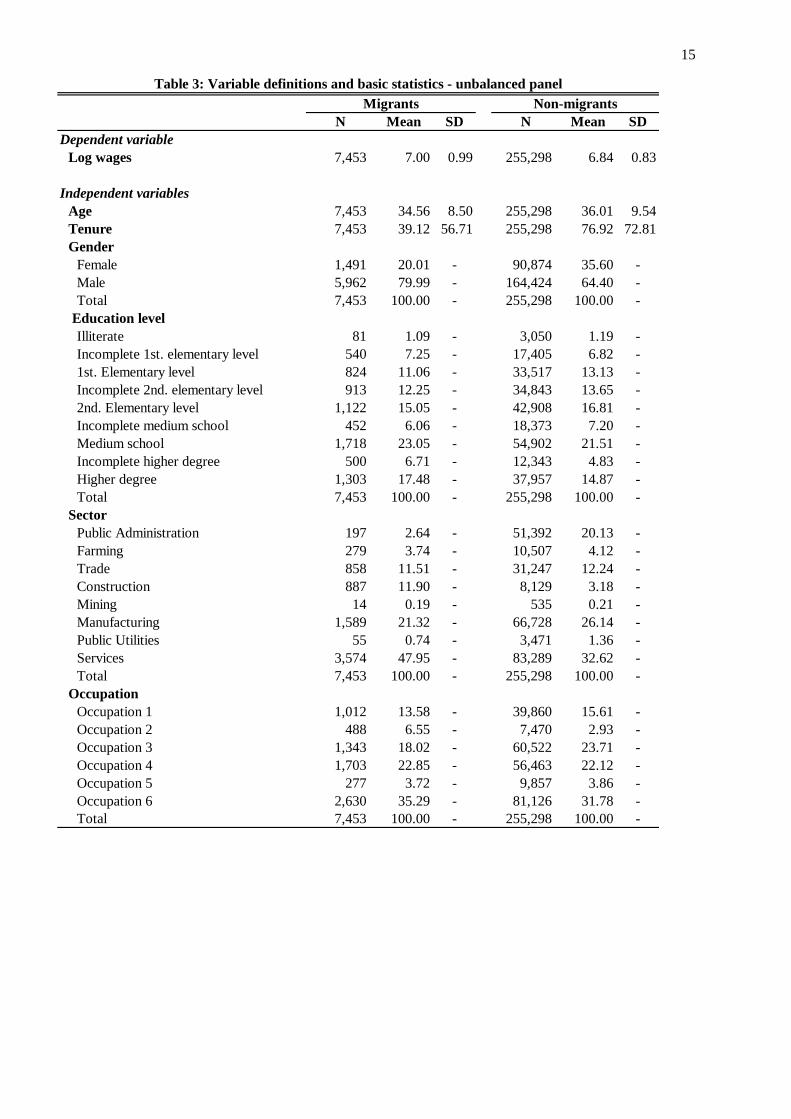
The most important contrast in the migrant characteristics between both panels is related to
qualification. The average tenure in the balanced panel is higher, and the education level as well.
Moreover, the share in qualified occupations is also higher. These evidences are corroborated by the
average wages of the balanced panel (R$2,400), which is higher than the average wages in the unbalanced
panel (R$1,881). Two additional characteristics can also be cited: the majority of males and the higher
share of the services sector (table 3). Then, we can conclude that the balanced panel has more skilled
workers than the unbalanced panel.
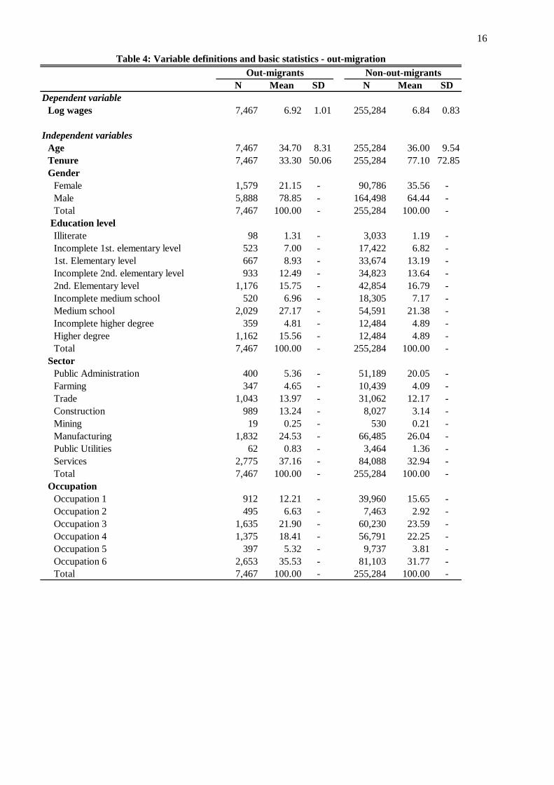
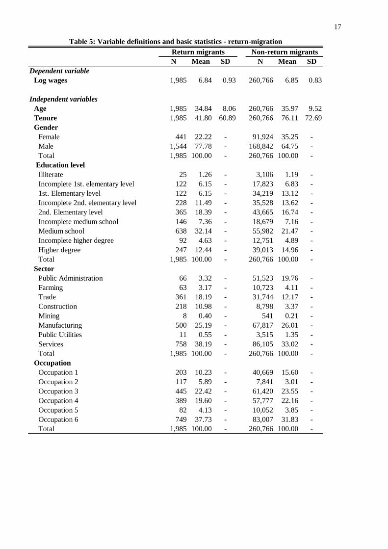
The features of the out-migrants can be observed in table 4. In general, these workers are 35 years
old, male (79%), with tenure of 2.8 years and high school (27%). They also work at service sector and in
blue-collar occupations, with an average wage of R$1,853. The subset of returning migrants, as we can
see in table 5, has more tenure, and has a higher share of high school (32%), but with a lower average
wage than out-migrants and also in-migrants (R$1.614).
<TABLE 2-5 ABOUT HERE>
3. Modeling the impact of migration on wages
In this section, the estimation procedure of wages considers the selection and the assimilation
under the individual fixed effects approach. The standard procedure in the majority of econometric
studies in the migration literature (Borjas, 1987, 1989, 1999; Chiswick, 1978; Chiswick et al., 2005) has
the Mincerian equation (Mincer, 1974) as the starting point:
Yit=Xitβt + δtMit + εit (1)
Yit is the log of worker wage i in the cross-section t (t=1995, ..., 2002);
Xit: vector of social and economical characteristics;
Mit: migration dummy (1 if migrant; 0 otherwise);
δt , βt: estimated coefficients;
εit: random error.
However, an important stylized fact in the economic literature is the self-selection of migrants. As
the migrants have personal characteristics, which make them different from other individuals, the formers
will have more wage gains than the others will. The methodological procedure that involves the
estimation of wage equations should consider this question, whose main point is related to the causality
attribution. According to the classical paper of Angrist and Krueger (1999), the ideal experiment could be
obtained with the observation of the same person in two different situations at the same time, and
controlling by other variables, which have effects on the wages. As stressed by Menezes-Filho (2001;
2002), the researcher would like to have the access to data with information about migrant wages before
and after the migration. This is the contra factual experiment that considers the wage differentials in a
causal way: the gains and/or losses after migration could be measured by a common test of means.
The point is that migrants are a self-selected group in comparison to the rest of the population.
Migrants have more probability to be successful even if they have not moved. The estimated wage
differentials probably will be biased, even using controls as age, tenure, gender, education, sector and
occupation. This kind of situation may occur because the observed controls used will not capture the
characteristics which may change the differences in wages between migrants and non-migrants.
5
The use of panel data allows a more effective solution to this problem than the use of aggregated
data. Using fixed individual effects in the panel dataset, we can estimate the mean effect of migration on
wages and compare the results for migrants and non-migrants (Booker et al., 2007). This is possible by
the establishment of an appropriated comparison set of non-migrants based on the random selection of
migrants (Peterson e Howell, 2003). Using this approach, it is not necessary to model the process by
which the migrants are self-selected, as in the pioneer study of Heckman (1979). Some studies considered
this selection problem using several controls, but they did not use panel data. The problem in these cases
is that they were not able to build a random selection. It is important to highlight that the fixed effects
method do not consider the situation of workers who can change some characteristics contemporaneously
with the migration (Hanushek et al., 2005). However, these changes will be a possible source of bias to
estimate just in case of a systematic pattern of episodes contemporaneous with the migration.
Using the longitudinal data of RAIS-Migra from 1995 to 2002, we can estimate the wage
equations to migrants and non-migrants in São Paulo state. The functional form of these regressions is as
following. The log wage is the dependent variable and the control variables are age, age squared, tenure,
tenure squared, and dummies of education, sector, occupation, year and gender. These independent
variables are subsumed in the X vector. The wage differentials associated to the migrants are δ, while θ
and λ are the wage differentials related to years since migration (YSMi e YSMi2). The time dummies are Tt,
and εi is the disturbance term, with variance ζε2. In order to deal with the endogeneity problem, we can
include a fixed effect, ci, in the regression. The identification hypothesis of the model asks for E(εi|ci, Mi ,
YSMi) = 0, i.e., the correlation between Mi, YSMi and εi is caught by a covariate which do not vary over
the years.2 Following, the traditional model that considers a quadratic assimilation curve:
ittiititititit TcYSMYSMMXY 2 (2)
It is important to notice that the abilities growth in the host region depends on duration, i.e., on the
years since migration. Therefore, ci and YSMi will be correlated if the non-observed ability of workers
shifts over the years. In this case, the OLS estimates of equation (2) will be biased. As we have a dataset
for eight years, we assumed that θ and λ do not change over years and by migrant cohorts as well. Then,
the fixed effect estimator is obtained by differencing the individual values of each variable and their mean
values. This procedure eliminates the ci term, avoiding possible effects of an individual ability bias. The
new estimates are consistent and efficient.
The main idea of this approach is to verify whether the longitudinal changes in wages can be
explained by M and YSM. In general, YSM and YSM2 have coefficients with undetermined signals. If θ>0
and λ>0, the relation between the wage distribution and YSM has an inverted U shaped form. It is
important to notice, however, that the hypothesis E(εi|ci, Mi , YSMi) = 0 may not be sufficient to eliminate
the endogeneity. It can appear in case of a random shock that causes a wage increase to workers anyway,
i.e., independently of them migrating or not.
4. Results
As the migrants are self-selected in comparison to the rest of the population, it is important to
consider the approach that includes the non-observable characteristics in the estimation process. In this
sense, the relative wages of migrants are estimated from a Mincerian equation, expanded by the gradual
inclusion of controls. This expansion starts with the inclusion of the observable characteristics until the
final inclusion of the fixed effects.
Furthermore, we evaluate the migrant assimilation in São Paulo. This is possible through the
inclusion of the variable years since migration. Using the fixed effects method, we can capture the real
migrant adjustment and avoid the self-selection bias. We also consider some robustness tests, analyzing
2 As a significant part of workers move to São Paulo over the years, the coefficients of wage differentials between migrants
and non-migrants can be identified after the inclusion of fixed effects.
6
the effects of migration on wages in several subsamples. Finally, we estimate the relative wages of people
who exit from São Paulo.
4.1. Evidences about the migrant self-selection
The following analysis uses different specifications to the X vector to estimate the wage
differentials of migrants in São Paulo. Tables 6 and 7 show us the results of the estimates by using the
balanced and the unbalanced panels, respectively. In general, we can confirm the existence of positive
selection of migrants in both panels. Therefore, it is necessary to consider the problems of self-selection
bias in order to obtain a correct estimate of migrant wages.
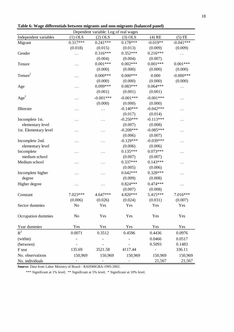
First considering the balanced panel (table 6), the three first columns show the OLS estimates,
while the two last ones show the random and the fixed effects estimates. In general, the wage returns are
higher when fewer controls are taken into account. These returns begin to decrease since more controls
are included in the regressions. For example, the log of migrant wages is 32% higher than the log of non-
migrant wages in model (1), whose unique covariates are the constant term and the year dummies.3
Following the sequence of models, the estimated coefficient falls to 24% in model (2), and to 18% in
model (3). These results, however, can be biased through the migrant self-selection. Therefore, we add
two other models to table 6 in order to solve this kind of problem. Using either the random effects or the
fixed effects model, the estimates converge to the same result: the coefficient turns to a negative signal,
which is significant at a 1% level. This can be interpreted as a migration in which the workers are not
absolutely aware about the costs related to the movement, especially to the cost of living in the host state.
As a result, the cost of living in São Paulo is an important cause of the estimated wage losses. In fact, the
cost of living in São Paulo is the highest, in average, among the metropolitan regions in Brazil from 1996
to 2002.
<TABLE 6 AND 7 ABOUT HERE>
It is important to observe that the individuals are present in the sample along the years as a whole
in the balanced panel. As several workers can stay in the host state for some years and then exit from the
formal labor market, the wage returns can be overestimated whether the balanced panel is considered.
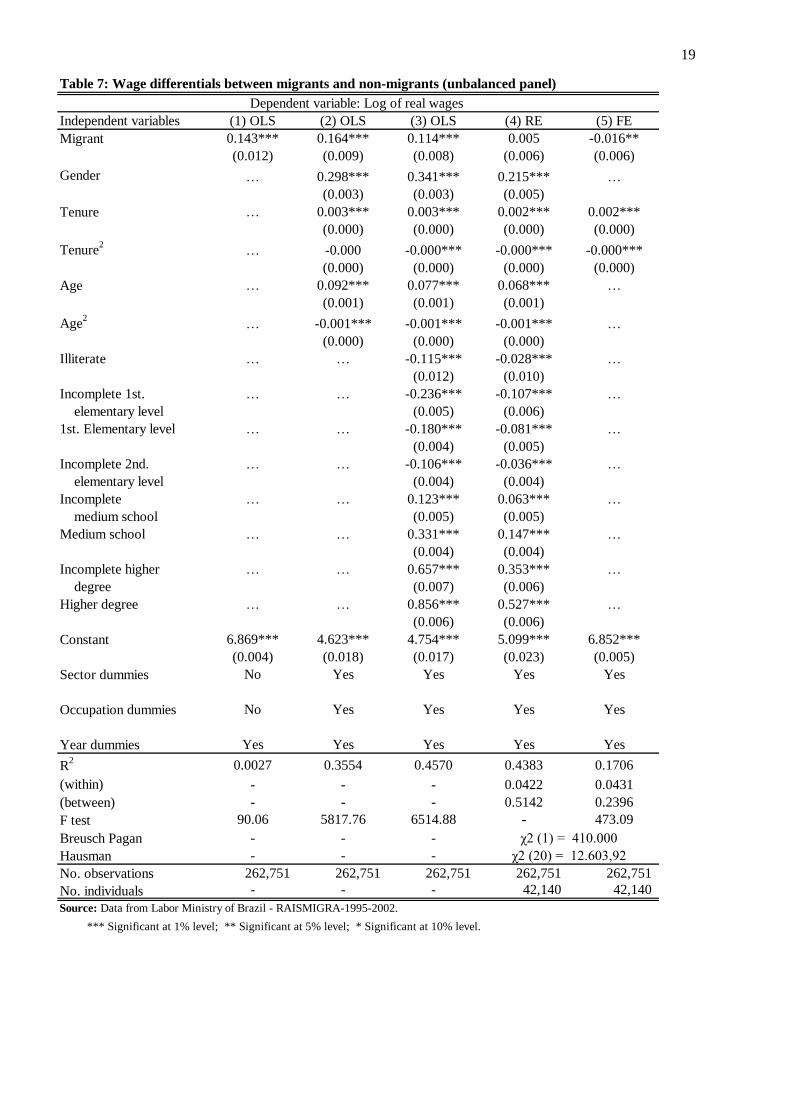
Then, we use the unbalanced panel in order to estimate the relative wages. As we can see in table 7,
whereas the relative wage of migrants in the regression (1) is 14% higher than the wages of other
workers, in regression (2) it is 16%, and in regression (3), which contains the education dummies, it is
just 11%. Following the same sequence of analysis of table 6, the random effects coefficient is not
significant at conventional statistic levels, and the inclusion of the fixed effects generates a negative wage
return. These results are different from those obtained using the balanced panel. A possible explanation is
that the balanced panel contains just the most skilled workers. In contrast, the unbalanced panel contains
all the movers and that who exit from a formal job. The results of the fixed effects model attest, in fact,
that the migrants from the unbalanced panel have less non-observable abilities than the migrants from the
balanced panel. Therefore, the forthcoming analysis will be based on the unbalanced panel.
An additional argument in favor to the use of the unbalanced panel is the Hausman test result. At
the bottom of table 7, we can observe the Hausman test using the unbalanced panel. The result rejects the
random effects model in favor to the fixed effects model.4 However, regarding to the balanced panel,
table 6 does not reports the Hausman test results because the model fitted on balanced sample fails to
meet the asymptotic assumptions of this test.
Overall, it is important to highlight that the relative wages after the control by the fixed effects
have a negative signal and are significant at the conventional statistic levels irrespective to the adopted
panel. The main result of this section answers to one of our previous questions. It shows that migrants
3 This wage percentage is calculated by [100(e(coef.)
–1)], that is equivalent to 38% in this case. However, we adopt the same
simplification of Borjas (1999), who uses the variation percentages in terms of logarithm differences. 4 Based on these results, the next estimates will report just the fixed effects model in this paper.
7
have relative wage losses of 1.6% after migration when their self-selection is taken into account by the
fixed effects model. This result contrasts strongly to that obtained by OLS, whose estimated coefficients
are positive, with wage gains of 11,5%. These returns are related to the positive selection of migrants,
since the OLS estimates do not capture the non-observable abilities of workers.
The wage losses that occur after the control of non-observable heterogeneity attest that the
workers move without the complete knowledge of the costs related to the migration. As an important
component of these costs is the cost of living in São Paulo, the expectation that workers have of enlarging
wages when living and working in São Paulo is not achieved. That is because the monetary illusion
derived from an imperfect set of information during their migration decision. As a result, some immediate
questions appear. How is the adjustment of these migrants in the labor market of the host state? Are the
initial losses persistent or are they overcome over the years? The answers to these questions sum to the
debate on the attendance necessity of the migration flows in the country and on the best composition of
individual qualifications to the migrants. Both topics are intrinsically related to the absorption capacity of
workers in São Paulo’s labor market.
4.2. Migrant assimilation
The main question of this section is to know how many years the migrant spend to amplify his/her
earnings in the host region. Although the worker has wage losses in moving to São Paulo, one may
acquire additional information about the host region throughout the years. For instance, he/she may know
what and where the jobs which pay more are.
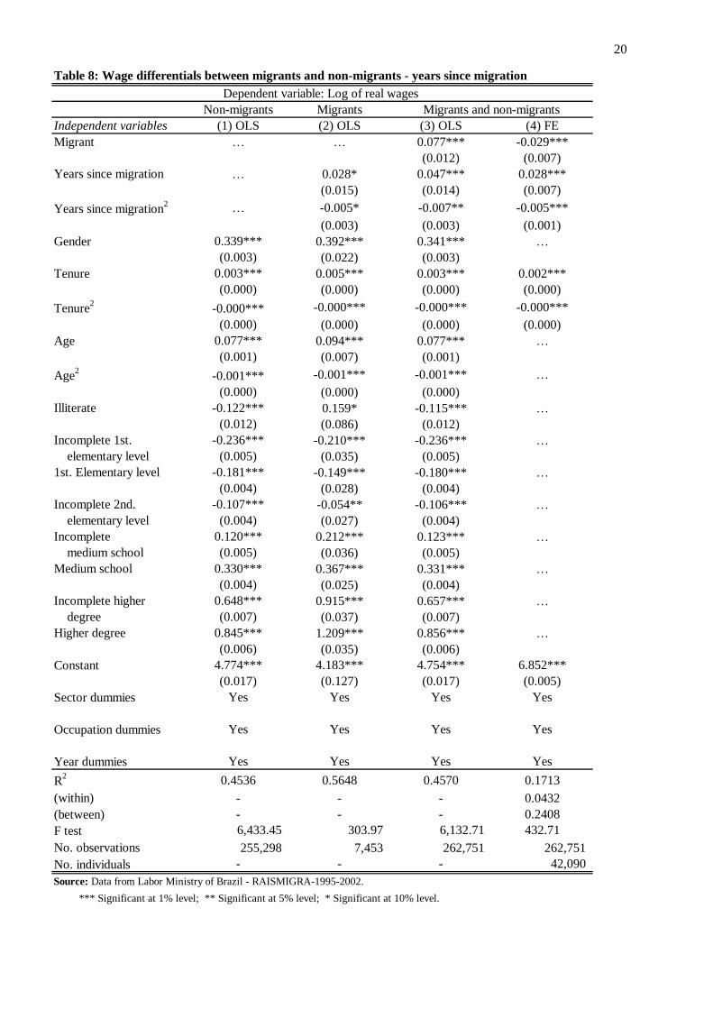
Table 8 presents some results on the migration adjustment of movers in São Paulo state.
Specifically, this adjustment is related to the coefficient of the years since migration variable. It shows
the wage distribution of workers according to the permanence in the host region. As the return resulting
from duration is also a question related the migrant self-selection, the control of non-observable abilities
is also necessary.
< TABLE 8 ABOUT HERE >
Firstly, we include the controls of the observable characteristics in the OLS regression. The
expected result of the assimilation effect on migrant wages is a consequence of the years in the host
country. However, the self-selection of migrants may bias the estimates. The non-observable
characteristics, such as ability, motivation, enterprising, etc., change among migrants and may explain a
large part of the gains associated to the duration. In this sense, the use of the fixed effects method helps to
the correct wage estimation of the migrants’ duration in São Paulo because we can control their non-
observable characteristics.
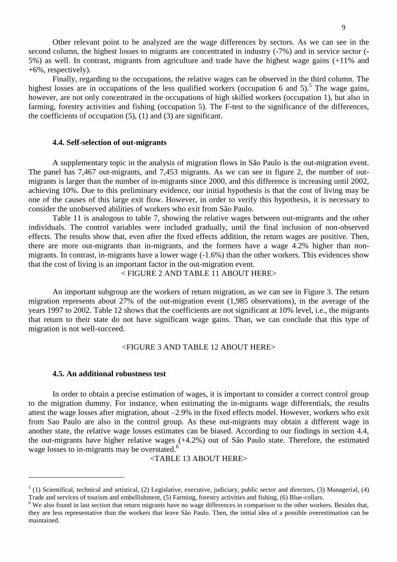
As we can see, models 1 to 4 in table 8 show the wage estimates to non-migrants, migrants, and to
the workers as a whole. On one hand, the results attest the wage losses after migration, since the partial
effect of migration on wages is –2.9% in the fixed effects model. On the other hand, there is a wage return
of +7.7% in the OLS model. However, the time since migration is an important variable on the
determination of migrants’ relative wages. In the OLS model, the coefficients of YSM and YSM2 are
significant at 1% level and coherent with the migration theory. The estimated values are +4.7% and –
0.7%, respectively, evidencing an inverted U-shaped curve. In contrast, the fixed effects model shows a
lower YSM coefficient of 2.8%. The quadratic component keeps the same negative signal, but reduces to –
0.5%. Therefore, the assimilation is overestimated in the OLS model. Considering the partial effect,
Y
M
–0.029 +0.028(YSM) –0.005(YSM)
2, the migrants’ adjustment happens under lower effects on
wages than the OLS estimation. Figure 1 clarifies this situation.
<FIGURE 1 ABOUT HERE>
8
In short, these results show that the earning convergence occurs 1.4 years after migration.
However, the wage growth happens with decreasing rates, within 3 years at most. As we have the control
of non-observable workers’ abilities, this fact can be a consequence of wage gains opportunities in São
Paulo. Therefore, the initial costs of migration, including the cost of living, causes a 2.9% fall on wages.
Additionally, there is a significance loss of the migration effect throughout time. We can conclude that
the information set of migrants is incomplete. On their migration decision, workers have a monetary
illusion because they see just the nominal wage, but not the real wage.
4.3. Migration effects in different samples
When a worker moves to São Paulo, there are wage losses in comparison to the non-migrants.
Several reasons can explain the wage losses after migration. Our hypothesis is that the decrease in wages
has the cost of living as an important cause. Then, what are the characteristics of workers with large wage
losses? Some groups can be more affected by these losses than others can.
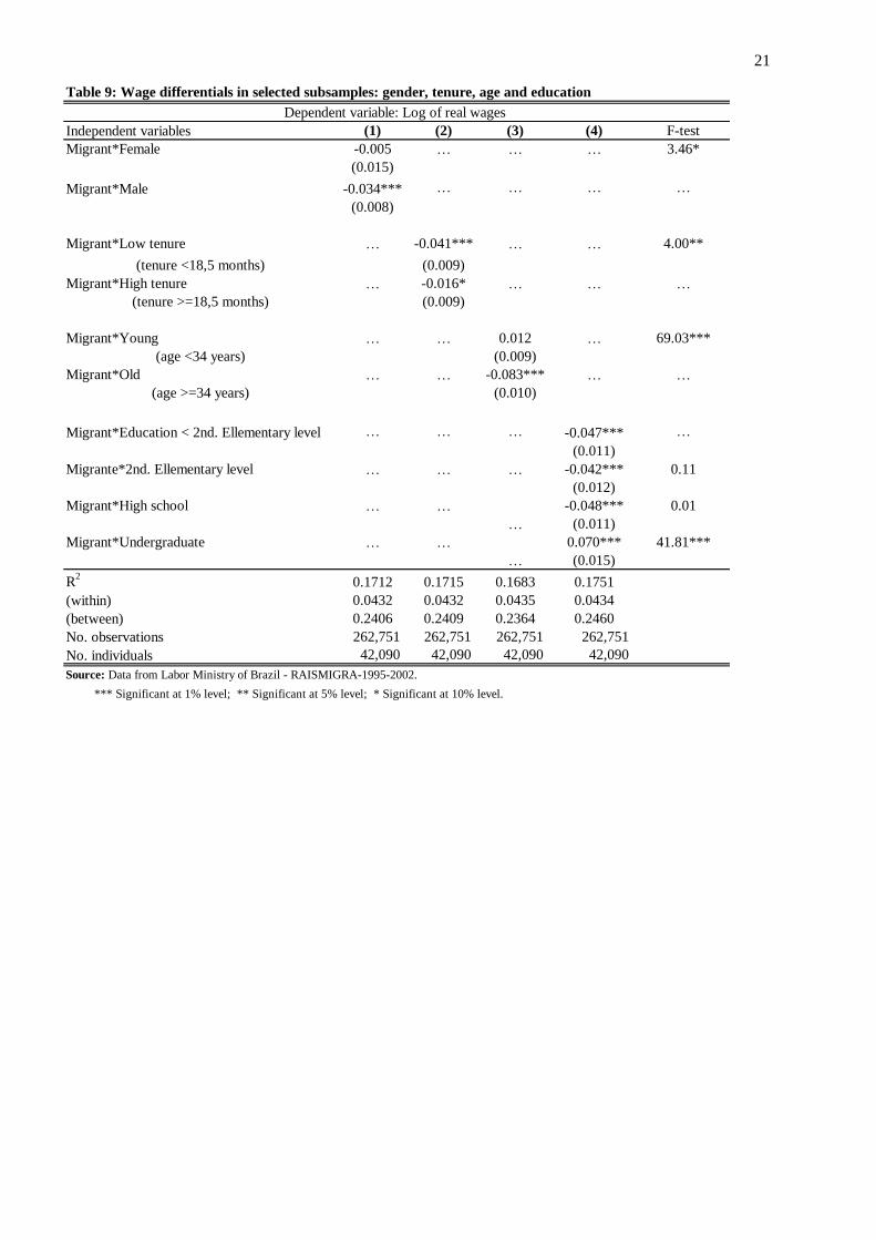
Table 9 compares relative wages of migrants in four different subsamples. The aim of this table is
to test the significance of wage differences among the selected groups: gender, tenure before migration,
age, and education). In the first column, we can see that there are wage differences of 3.4% for the
migrant men in comparison to the non-migrants. This difference is also significant in comparison to the
migrant women, but just at the level of 10%.
<TABLE 9 ABOUT HERE>
The second column shows the estimates of migrant wage differentials according to the job tenure
before migration. The migrants with more tenure are that with job tenure higher than 18.5 months. The
wage differences between the both groups are significant at 5% level, as we can see in the F-test in the
last column of the table. While the losses to the less experienced workers are at 4.1%, those with more
tenure have losses of just 1.6%.
In the subsample that characterizes the wage differentials by age (third column), the wage return
of the young migrants is higher than that of the old ones. The old migrants have wages 8.3% less than that
of non-migrants, and this difference is statistically significant, as we can see in the last column. These
higher losses to the old migrants can be related to the short period they have to obtain the return of the
migration investment.
In column (4), we compared the wage differentials between migrants and non-migrants by
educational levels. According to the human capital model, the more educated workers can be more
efficient in finding and evaluating job opportunities. As a result, they can reduce the migration costs. The
results show that there is a large contrast between high educated and low educated workers. On one hand,
the group of migrants less educated has losses of 5% in comparison to the non-migrants. On the other
hand, the migrants with high education earn 7% more than non-migrants. We can conclude that there are
vacancies to more qualified workers in the labor market.
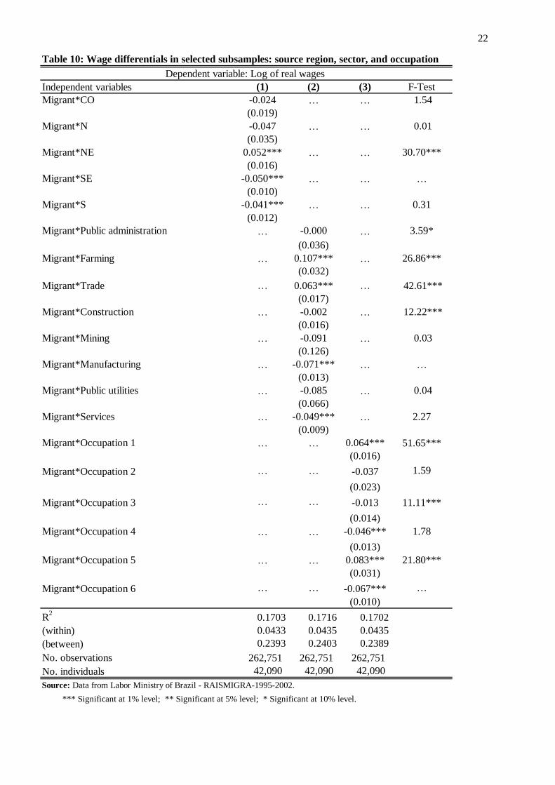
Another important issue to be analyzed is the geographical distribution of the relative wage of
migrants according to their source region, sector and occupation. This is the main idea of table 10, which
compares the estimated wages in three different subsamples. First considering the source region, the
results can be observed in the first column. The wage losses after migration can be observed to movers
who come from other states of Southeast region (-5%), followed by those movers from the South region
(-4%). On the other hand, migrants from the Northeast region have positive wage returns of 5.2%. These
effects are related to the real wage correction. When the Northeast workers move to São Paulo, they have
real wage gains. Considering the F test, in the last column, only the differences between the Southeast and
the Northeast are significant at conventional statistic levels. Then, the high cost of living between these
two regions is an important factor to the high earning inequality of the country.
<TABLE 10 ABOUT HERE>
9
Other relevant point to be analyzed are the wage differences by sectors. As we can see in the
second column, the highest losses to migrants are concentrated in industry (-7%) and in service sector (-
5%) as well. In contrast, migrants from agriculture and trade have the highest wage gains (+11% and
+6%, respectively).
Finally, regarding to the occupations, the relative wages can be observed in the third column. The
highest losses are in occupations of the less qualified workers (occupation 6 and 5).5 The wage gains,
however, are not only concentrated in the occupations of high skilled workers (occupation 1), but also in
farming, forestry activities and fishing (occupation 5). The F-test to the significance of the differences,
the coefficients of occupation (5), (1) and (3) are significant.
4.4. Self-selection of out-migrants
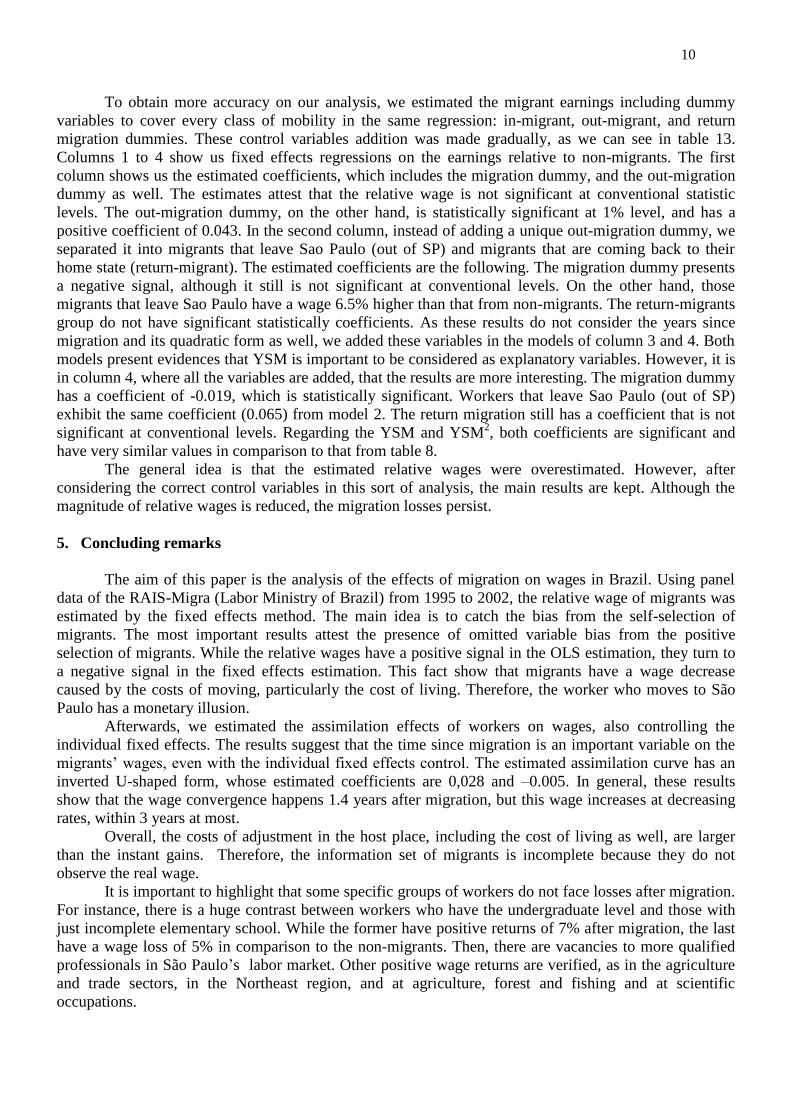
A supplementary topic in the analysis of migration flows in São Paulo is the out-migration event.
The panel has 7,467 out-migrants, and 7,453 migrants. As we can see in figure 2, the number of out-
migrants is larger than the number of in-migrants since 2000, and this difference is increasing until 2002,
achieving 10%. Due to this preliminary evidence, our initial hypothesis is that the cost of living may be
one of the causes of this large exit flow. However, in order to verify this hypothesis, it is necessary to
consider the unobserved abilities of workers who exit from São Paulo.
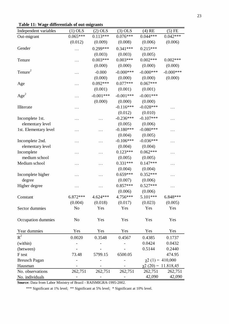
Table 11 is analogous to table 7, showing the relative wages between out-migrants and the other
individuals. The control variables were included gradually, until the final inclusion of non-observed
effects. The results show that, even after the fixed effects addition, the return wages are positive. Then,
there are more out-migrants than in-migrants, and the formers have a wage 4.2% higher than non-
migrants. In contrast, in-migrants have a lower wage (-1.6%) than the other workers. This evidences show
that the cost of living is an important factor in the out-migration event.
< FIGURE 2 AND TABLE 11 ABOUT HERE>
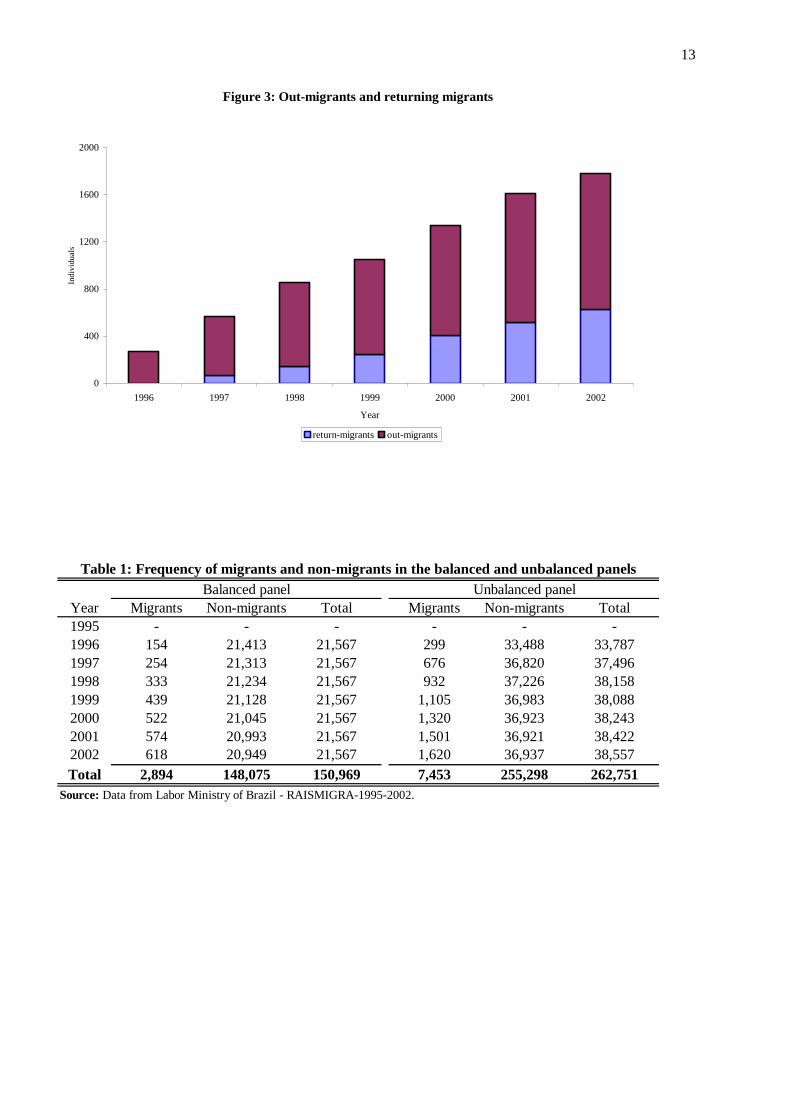
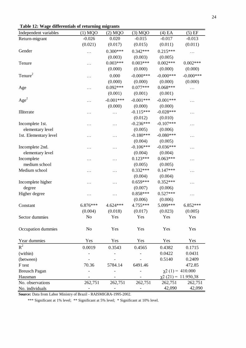
An important subgroup are the workers of return migration, as we can see in Figure 3. The return
migration represents about 27% of the out-migration event (1,985 observations), in the average of the
years 1997 to 2002. Table 12 shows that the coefficients are not significant at 10% level, i.e., the migrants
that return to their state do not have significant wage gains. Than, we can conclude that this type of
migration is not well-succeed.
<FIGURE 3 AND TABLE 12 ABOUT HERE>
4.5. An additional robustness test
In order to obtain a precise estimation of wages, it is important to consider a correct control group
to the migration dummy. For instance, when estimating the in-migrants wage differentials, the results
attest the wage losses after migration, about –2.9% in the fixed effects model. However, workers who exit
from Sao Paulo are also in the control group. As these out-migrants may obtain a different wage in
another state, the relative wage losses estimates can be biased. According to our findings in section 4.4,
the out-migrants have higher relative wages (+4.2%) out of São Paulo state. Therefore, the estimated
wage losses to in-migrants may be overstated.6
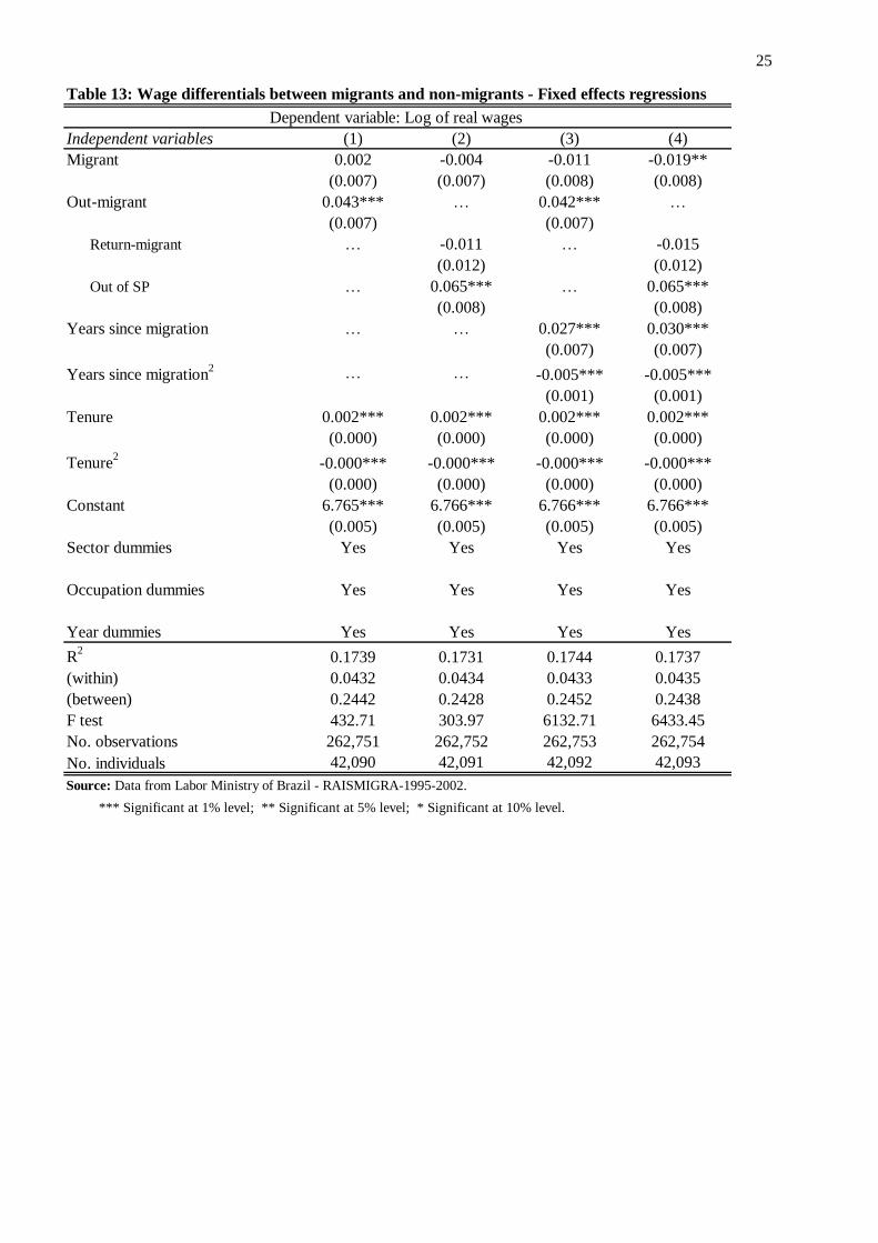
<TABLE 13 ABOUT HERE>
5 (1) Scientifical, technical and artistical, (2) Legislative, executive, judiciary, public sector and directors, (3) Managerial, (4)
Trade and services of tourism and embellishment, (5) Farming, forestry activities and fishing, (6) Blue-collars. 6 We also found in last section that return migrants have no wage differences in comparison to the other workers. Besides that,
they are less representative than the workers that leave São Paulo. Then, the initial idea of a possible overestimation can be
maintained.
10
To obtain more accuracy on our analysis, we estimated the migrant earnings including dummy
variables to cover every class of mobility in the same regression: in-migrant, out-migrant, and return
migration dummies. These control variables addition was made gradually, as we can see in table 13.
Columns 1 to 4 show us fixed effects regressions on the earnings relative to non-migrants. The first
column shows us the estimated coefficients, which includes the migration dummy, and the out-migration
dummy as well. The estimates attest that the relative wage is not significant at conventional statistic
levels. The out-migration dummy, on the other hand, is statistically significant at 1% level, and has a
positive coefficient of 0.043. In the second column, instead of adding a unique out-migration dummy, we
separated it into migrants that leave Sao Paulo (out of SP) and migrants that are coming back to their
home state (return-migrant). The estimated coefficients are the following. The migration dummy presents
a negative signal, although it still is not significant at conventional levels. On the other hand, those
migrants that leave Sao Paulo have a wage 6.5% higher than that from non-migrants. The return-migrants
group do not have significant statistically coefficients. As these results do not consider the years since
migration and its quadratic form as well, we added these variables in the models of column 3 and 4. Both
models present evidences that YSM is important to be considered as explanatory variables. However, it is
in column 4, where all the variables are added, that the results are more interesting. The migration dummy
has a coefficient of -0.019, which is statistically significant. Workers that leave Sao Paulo (out of SP)
exhibit the same coefficient (0.065) from model 2. The return migration still has a coefficient that is not
significant at conventional levels. Regarding the YSM and YSM2, both coefficients are significant and
have very similar values in comparison to that from table 8.
The general idea is that the estimated relative wages were overestimated. However, after
considering the correct control variables in this sort of analysis, the main results are kept. Although the
magnitude of relative wages is reduced, the migration losses persist.
5. Concluding remarks
The aim of this paper is the analysis of the effects of migration on wages in Brazil. Using panel
data of the RAIS-Migra (Labor Ministry of Brazil) from 1995 to 2002, the relative wage of migrants was
estimated by the fixed effects method. The main idea is to catch the bias from the self-selection of
migrants. The most important results attest the presence of omitted variable bias from the positive
selection of migrants. While the relative wages have a positive signal in the OLS estimation, they turn to
a negative signal in the fixed effects estimation. This fact show that migrants have a wage decrease
caused by the costs of moving, particularly the cost of living. Therefore, the worker who moves to São
Paulo has a monetary illusion.
Afterwards, we estimated the assimilation effects of workers on wages, also controlling the
individual fixed effects. The results suggest that the time since migration is an important variable on the
migrants’ wages, even with the individual fixed effects control. The estimated assimilation curve has an
inverted U-shaped form, whose estimated coefficients are 0,028 and –0.005. In general, these results
show that the wage convergence happens 1.4 years after migration, but this wage increases at decreasing
rates, within 3 years at most.
Overall, the costs of adjustment in the host place, including the cost of living as well, are larger
than the instant gains. Therefore, the information set of migrants is incomplete because they do not
observe the real wage.
It is important to highlight that some specific groups of workers do not face losses after migration.
For instance, there is a huge contrast between workers who have the undergraduate level and those with
just incomplete elementary school. While the former have positive returns of 7% after migration, the last
have a wage loss of 5% in comparison to the non-migrants. Then, there are vacancies to more qualified
professionals in São Paulo’s labor market. Other positive wage returns are verified, as in the agriculture
and trade sectors, in the Northeast region, and at agriculture, forest and fishing and at scientific
occupations.
11
Finally, the wage returns were also estimated to the out-migrants. Even after the fixed effects
inclusion, there are positive gains. The return migration, a subset of out-migrants, does not have
significant gains at 1% level. Therefore, our results are consistent with the fact that the high cost of living
in São Paulo can bring back migrants to their source place, and also generate an out-migration from São
Paulo to other Brazilian states.
6. References
ANGRIST, J. and KRUEGER, A. (1999) Empirical strategies in labor economics. In: ASHENFELTER,
O. and CARD, D. Handbook of labor economics. Elsevier, v. 3A.
AZZONI, C. et al. (2003) Comparações da Paridade do Poder de Compra entre cidades: aspectos
metodológicos e aplicação ao caso brasileiro. Pesquisa e Planejamento Econômico, v. 33, n. 1.
BOOKER, K. et al. (2007). The impact of charter school attendance on student performance. Journal of
Public Economics, v. 91, p. 849–876.
BORJAS, G. Self-Selection and the Earnings of Immigrants. (1987) American Economic Review, v.
77(4), p. 531-553.
_________. Immigrant and emigrant earnings: a longitudinal study. (1989) Economic Inquiry, 27:21-
37, 1989.
_________. The Economic Analysis of Immigration. (1999) Handbook of Labor Economics, vol. 3.
CHISWICK, B. R. The Effect of Americanization on the Earnings of Foreign-Born Men. (1978), Journal
of Political Economy, v. 86, p. 897- 921.
CHISWICK, B. R.; LEE, Y. L.; MILLER P.W. (2005) Longitudinal analysis of immigrant occupational
mobility: A test of the immigrant assimilation hypothesis, International Migration Review, v. 39, n.2.
HECKMAN, J. Sample selection bias as a specification error. (1979) Econometrica, v. 47, n. 1, p. 153-
161.
MENEZES-FILHO, N. (2002) Equações de rendimentos: questões metodológicas. In: CORSEUIL, C. H.
et al (Orgs). Estrutura salarial: aspectos conceituais e novos resultados para o Brasil. Rio de Janeiro:
IPEA.
MENEZES-FILHO, N. Microeconometria. (2001) In: LISBOA, M. E MENEZES-FILHO, N.
Microeconomia e sociedade no Brasil. Rio de Janeiro: Editora Contra-capa.
MINCER, J. Schooling, experience and earnings. (1974) New York: National Bureau for Economic
Research.
MINISTÉRIO DO TRABALHO E EMPREGO. (2003) Raismigra: modelos painel e vínculo –
orientações para uso. (Manuscript).
MINISTÉRIO DO TRABALHO E EMPREGO. Raismigra. (1995-2002). Brasília: MTE.
12
PETERSON, Paul E.; HOWELL, WILLIAM G. (2003) Latest results from the New York City
voucher experiment. Harvard University Working Paper.
FIGURES AND TABLES
Figure 1: The effects of assimilation on wages
-0.050
0.000
0.050
0.100
0.150
0.200
0 1 2 3 4 5 6
Years since migration
Wag
e v
ari
ati
on
OLS FE
Figure 2: Out-migrants vs. In-migrants
0
400
800
1200
1600
2000
1996 1997 1998 1999 2000 2001 2002
Year
Ind
ivid
ual
s
Out-migrants In-migrants
13
Figure 3: Out-migrants and returning migrants
0
400
800
1200
1600
2000
1996 1997 1998 1999 2000 2001 2002
Year
Indiv
idual
s
return-migrants out-migrants
Year Migrants Non-migrants Total Migrants Non-migrants Total
1995 - - - - - -
1996 154 21,413 21,567 299 33,488 33,787
1997 254 21,313 21,567 676 36,820 37,496
1998 333 21,234 21,567 932 37,226 38,158
1999 439 21,128 21,567 1,105 36,983 38,088
2000 522 21,045 21,567 1,320 36,923 38,243
2001 574 20,993 21,567 1,501 36,921 38,422
2002 618 20,949 21,567 1,620 36,937 38,557
Total 2,894 148,075 150,969 7,453 255,298 262,751
Source: Data from Labor Ministry of Brazil - RAISMIGRA-1995-2002.
Table 1: Frequency of migrants and non-migrants in the balanced and unbalanced panels
Balanced panel Unbalanced panel
14
N Mean SD N Mean SD
Dependent variable
Log wages 2,894 7.31 0.98 148,075 6.98 0.83
Independent variables
Age 2,894 35.46 8.20 148,075 37.33 9.40
Tenure 2,894 58.30 69.44 148,075 97.79 75.48
Gender
Female 552 19.07 - 57,551 38.87 -
Male 2,342 80.93 - 90,524 61.13 -
Total 2,894 100.00 - 148,075 100.00 -
Education level
Illiterate 45 1.55 - 1,691 1.14 -
Incomplete 1st. elementary level 166 5.74 - 9,108 6.15 -
1st. Elementary level 270 9.33 - 18,607 12.57 -
Incomplete 2nd. elementary level 285 9.85 - 18,308 12.36 -
2nd. Elementary level 358 12.37 - 22,834 15.42 -
Incomplete medium school 149 5.15 - 9,757 6.59 -
Medium school 723 24.98 - 33,259 22.46 -
Incomplete higher degree 231 7.98 - 7,868 5.31 -
Higher degree 667 23.05 - 26,643 17.99 -
Total 2,894 100.00 - 148,075 100.00 -
Sector
Public Administration 84 2.90 - 39,947 26.98 -
Farming 61 2.11 - 4,647 3.14 -
Trade 270 9.33 - 13,582 9.17 -
Construction 178 6.15 - 2,592 1.75 -
Mining 0 0.00 - 258 0.17 -
Manufacturing 736 25.43 - 37,141 25.08 -
Public Utilities 27 0.93 - 2,675 1.81 -
Services 1,538 53.14 - 47,233 31.90 -
Total 2,894 100.00 - 148,075 100.00 -
Occupation
Occupation 1 501 19.08 - 28,255 19.08 -
Occupation 2 248 3.29 - 4,872 3.29 -
Occupation 3 561 19.38 - 38,273 25.85 -
Occupation 4 624 21.56 - 30,472 20.58 -
Occupation 5 55 1.90 - 4,195 2.83 -
Occupation 6 905 31.27 - 42,008 28.37 -
Total 2,894 100.00 - 148,075 100.00 -
Non-migrantsMigrants
Table 2: Variable definitions and basic statistics - balanced panel
15
N Mean SD N Mean SD
Dependent variable
Log wages 7,453 7.00 0.99 255,298 6.84 0.83
Independent variables
Age 7,453 34.56 8.50 255,298 36.01 9.54
Tenure 7,453 39.12 56.71 255,298 76.92 72.81
Gender
Female 1,491 20.01 - 90,874 35.60 -
Male 5,962 79.99 - 164,424 64.40 -
Total 7,453 100.00 - 255,298 100.00 -
Education level
Illiterate 81 1.09 - 3,050 1.19 -
Incomplete 1st. elementary level 540 7.25 - 17,405 6.82 -
1st. Elementary level 824 11.06 - 33,517 13.13 -
Incomplete 2nd. elementary level 913 12.25 - 34,843 13.65 -
2nd. Elementary level 1,122 15.05 - 42,908 16.81 -
Incomplete medium school 452 6.06 - 18,373 7.20 -
Medium school 1,718 23.05 - 54,902 21.51 -
Incomplete higher degree 500 6.71 - 12,343 4.83 -
Higher degree 1,303 17.48 - 37,957 14.87 -
Total 7,453 100.00 - 255,298 100.00 -
Sector
Public Administration 197 2.64 - 51,392 20.13 -
Farming 279 3.74 - 10,507 4.12 -
Trade 858 11.51 - 31,247 12.24 -
Construction 887 11.90 - 8,129 3.18 -
Mining 14 0.19 - 535 0.21 -
Manufacturing 1,589 21.32 - 66,728 26.14 -
Public Utilities 55 0.74 - 3,471 1.36 -
Services 3,574 47.95 - 83,289 32.62 -
Total 7,453 100.00 - 255,298 100.00 -
Occupation
Occupation 1 1,012 13.58 - 39,860 15.61 -
Occupation 2 488 6.55 - 7,470 2.93 -
Occupation 3 1,343 18.02 - 60,522 23.71 -
Occupation 4 1,703 22.85 - 56,463 22.12 -
Occupation 5 277 3.72 - 9,857 3.86 -
Occupation 6 2,630 35.29 - 81,126 31.78 -
Total 7,453 100.00 - 255,298 100.00 -
Table 3: Variable definitions and basic statistics - unbalanced panel
Non-migrantsMigrants
16
N Mean SD N Mean SD
Dependent variable
Log wages 7,467 6.92 1.01 255,284 6.84 0.83
Independent variables
Age 7,467 34.70 8.31 255,284 36.00 9.54
Tenure 7,467 33.30 50.06 255,284 77.10 72.85
Gender
Female 1,579 21.15 - 90,786 35.56 -
Male 5,888 78.85 - 164,498 64.44 -
Total 7,467 100.00 - 255,284 100.00 -
Education level
Illiterate 98 1.31 - 3,033 1.19 -
Incomplete 1st. elementary level 523 7.00 - 17,422 6.82 -
1st. Elementary level 667 8.93 - 33,674 13.19 -
Incomplete 2nd. elementary level 933 12.49 - 34,823 13.64 -
2nd. Elementary level 1,176 15.75 - 42,854 16.79 -
Incomplete medium school 520 6.96 - 18,305 7.17 -
Medium school 2,029 27.17 - 54,591 21.38 -
Incomplete higher degree 359 4.81 - 12,484 4.89 -
Higher degree 1,162 15.56 - 12,484 4.89 -
Total 7,467 100.00 - 255,284 100.00 -
Sector
Public Administration 400 5.36 - 51,189 20.05 -
Farming 347 4.65 - 10,439 4.09 -
Trade 1,043 13.97 - 31,062 12.17 -
Construction 989 13.24 - 8,027 3.14 -
Mining 19 0.25 - 530 0.21 -
Manufacturing 1,832 24.53 - 66,485 26.04 -
Public Utilities 62 0.83 - 3,464 1.36 -
Services 2,775 37.16 - 84,088 32.94 -
Total 7,467 100.00 - 255,284 100.00 -
Occupation
Occupation 1 912 12.21 - 39,960 15.65 -
Occupation 2 495 6.63 - 7,463 2.92 -
Occupation 3 1,635 21.90 - 60,230 23.59 -
Occupation 4 1,375 18.41 - 56,791 22.25 -
Occupation 5 397 5.32 - 9,737 3.81 -
Occupation 6 2,653 35.53 - 81,103 31.77 -
Total 7,467 100.00 - 255,284 100.00 -
Table 4: Variable definitions and basic statistics - out-migration
Non-out-migrantsOut-migrants
17
N Mean SD N Mean SD
Dependent variable
Log wages 1,985 6.84 0.93 260,766 6.85 0.83
Independent variables
Age 1,985 34.84 8.06 260,766 35.97 9.52
Tenure 1,985 41.80 60.89 260,766 76.11 72.69
Gender
Female 441 22.22 - 91,924 35.25 -
Male 1,544 77.78 - 168,842 64.75 -
Total 1,985 100.00 - 260,766 100.00 -
Education level
Illiterate 25 1.26 - 3,106 1.19 -
Incomplete 1st. elementary level 122 6.15 - 17,823 6.83 -
1st. Elementary level 122 6.15 - 34,219 13.12 -
Incomplete 2nd. elementary level 228 11.49 - 35,528 13.62 -
2nd. Elementary level 365 18.39 - 43,665 16.74 -
Incomplete medium school 146 7.36 - 18,679 7.16 -
Medium school 638 32.14 - 55,982 21.47 -
Incomplete higher degree 92 4.63 - 12,751 4.89 -
Higher degree 247 12.44 - 39,013 14.96 -
Total 1,985 100.00 - 260,766 100.00 -
Sector
Public Administration 66 3.32 - 51,523 19.76 -
Farming 63 3.17 - 10,723 4.11 -
Trade 361 18.19 - 31,744 12.17 -
Construction 218 10.98 - 8,798 3.37 -
Mining 8 0.40 - 541 0.21 -
Manufacturing 500 25.19 - 67,817 26.01 -
Public Utilities 11 0.55 - 3,515 1.35 -
Services 758 38.19 - 86,105 33.02 -
Total 1,985 100.00 - 260,766 100.00 -
Occupation
Occupation 1 203 10.23 - 40,669 15.60 -
Occupation 2 117 5.89 - 7,841 3.01 -
Occupation 3 445 22.42 - 61,420 23.55 -
Occupation 4 389 19.60 - 57,777 22.16 -
Occupation 5 82 4.13 - 10,052 3.85 -
Occupation 6 749 37.73 - 83,007 31.83 -
Total 1,985 100.00 - 260,766 100.00 -
Table 5: Variable definitions and basic statistics - return-migration
Non-return migrantsReturn migrants
18
Table 6: Wage differentials between migrants and non-migrants (balanced panel)
Independent variables (1) OLS (2) OLS (3) OLS (4) RE (5) FE
Migrant 0.317*** 0.241*** 0.178*** -0.019** -0.041***
(0.018) (0.015) (0.013) (0.009) (0.009)
Gender … 0.316*** 0.352*** 0.216*** …
(0.004) (0.004) (0.007)
Tenure … 0.001*** 0.002*** 0.001*** 0.001***
(0.000) (0.000) (0.000) (0.000)
Tenure2
… 0.000*** 0.000*** 0.000 -0.000***
(0.000) (0.000) (0.000) (0.000)
Age … 0.099*** 0.083*** 0.064*** …
(0.001) (0.001) (0.001)
Age2
… -0.001*** -0.001*** -0.001*** …
(0.000) (0.000) (0.000)
Illiterate … … -0.140*** -0.042*** …
(0.017) (0.014)
Incomplete 1st. … … -0.250*** -0.113*** …
elementary level (0.007) (0.008)
1st. Elementary level … … -0.208*** -0.085*** …
(0.006) (0.007)
Incomplete 2nd. … … -0.129*** -0.039*** …
elementary level (0.006) (0.006)
Incomplete … … 0.135*** 0.073*** …
medium school (0.007) (0.007)
Medium school … … 0.337*** 0.143*** …
(0.005) (0.006)
Incomplete higher … … 0.642*** 0.328*** …
degree (0.009) (0.008)
Higher degree … … 0.824*** 0.474*** …
(0.007) (0.008)
Constant 7.023*** 4.647*** 4.820*** 5.415*** 7.016***
(0.006) (0.026) (0.024) (0.031) (0.007)
Sector dummies No Yes Yes Yes Yes
Occupation dummies No Yes Yes Yes Yes
Year dummies Yes Yes Yes Yes Yes
R2
0.0071 0.3512 0.4596 0.4436 0.0976
(within) - - - 0.0466 0.0517
(between) - - - 0.5093 0.1483
F test 135.69 3521.58 4117.44 - 336.11
No. observations 150,969 150,969 150,969 150,969 150,969
No. individuals - - - 21,567 21,567
Source: Data from Labor Ministry of Brazil - RAISMIGRA-1995-2002.
*** Significant at 1% level; ** Significant at 5% level; * Significant at 10% level.
Dependent variable: Log of real wages
19
Table 7: Wage differentials between migrants and non-migrants (unbalanced panel)
Independent variables (1) OLS (2) OLS (3) OLS (4) RE (5) FE
Migrant 0.143*** 0.164*** 0.114*** 0.005 -0.016**
(0.012) (0.009) (0.008) (0.006) (0.006)
Gender … 0.298*** 0.341*** 0.215*** …
(0.003) (0.003) (0.005)
Tenure … 0.003*** 0.003*** 0.002*** 0.002***
(0.000) (0.000) (0.000) (0.000)
Tenure2
… -0.000 -0.000*** -0.000*** -0.000***
(0.000) (0.000) (0.000) (0.000)
Age … 0.092*** 0.077*** 0.068*** …
(0.001) (0.001) (0.001)
Age2
… -0.001*** -0.001*** -0.001*** …
(0.000) (0.000) (0.000)
Illiterate … … -0.115*** -0.028*** …
(0.012) (0.010)
Incomplete 1st. … … -0.236*** -0.107*** …
elementary level (0.005) (0.006)
1st. Elementary level … … -0.180*** -0.081*** …
(0.004) (0.005)
Incomplete 2nd. … … -0.106*** -0.036*** …
elementary level (0.004) (0.004)
Incomplete … … 0.123*** 0.063*** …
medium school (0.005) (0.005)
Medium school … … 0.331*** 0.147*** …
(0.004) (0.004)
Incomplete higher … … 0.657*** 0.353*** …
degree (0.007) (0.006)
Higher degree … … 0.856*** 0.527*** …
(0.006) (0.006)
Constant 6.869*** 4.623*** 4.754*** 5.099*** 6.852***
(0.004) (0.018) (0.017) (0.023) (0.005)
Sector dummies No Yes Yes Yes Yes
Occupation dummies No Yes Yes Yes Yes
Year dummies Yes Yes Yes Yes Yes
R2
0.0027 0.3554 0.4570 0.4383 0.1706
(within) - - - 0.0422 0.0431
(between) - - - 0.5142 0.2396
F test 90.06 5817.76 6514.88 - 473.09
Breusch Pagan - - -
Hausman - - -
No. observations 262,751 262,751 262,751 262,751 262,751
No. individuals - - - 42,140 42,140
Source: Data from Labor Ministry of Brazil - RAISMIGRA-1995-2002.
*** Significant at 1% level; ** Significant at 5% level; * Significant at 10% level.
Dependent variable: Log of real wages
χ2 (1) = 410.000
χ2 (20) = 12.603,92
20
Table 8: Wage differentials between migrants and non-migrants - years since migration
Non-migrants Migrants
Independent variables (1) OLS (2) OLS (3) OLS (4) FE
Migrant … … 0.077*** -0.029***
(0.012) (0.007)
Years since migration … 0.028* 0.047*** 0.028***
(0.015) (0.014) (0.007)
Years since migration2 … -0.005* -0.007** -0.005***
(0.003) (0.003) (0.001)
Gender 0.339*** 0.392*** 0.341*** …
(0.003) (0.022) (0.003)
Tenure 0.003*** 0.005*** 0.003*** 0.002***
(0.000) (0.000) (0.000) (0.000)
Tenure2
-0.000*** -0.000*** -0.000*** -0.000***
(0.000) (0.000) (0.000) (0.000)
Age 0.077*** 0.094*** 0.077*** …
(0.001) (0.007) (0.001)
Age2
-0.001*** -0.001*** -0.001*** …
(0.000) (0.000) (0.000)
Illiterate -0.122*** 0.159* -0.115*** …
(0.012) (0.086) (0.012)
Incomplete 1st. -0.236*** -0.210*** -0.236*** …
elementary level (0.005) (0.035) (0.005)
1st. Elementary level -0.181*** -0.149*** -0.180*** …
(0.004) (0.028) (0.004)
Incomplete 2nd. -0.107*** -0.054** -0.106*** …
elementary level (0.004) (0.027) (0.004)
Incomplete 0.120*** 0.212*** 0.123*** …
medium school (0.005) (0.036) (0.005)
Medium school 0.330*** 0.367*** 0.331*** …
(0.004) (0.025) (0.004)
Incomplete higher 0.648*** 0.915*** 0.657*** …
degree (0.007) (0.037) (0.007)
Higher degree 0.845*** 1.209*** 0.856*** …
(0.006) (0.035) (0.006)
Constant 4.774*** 4.183*** 4.754*** 6.852***
(0.017) (0.127) (0.017) (0.005)
Sector dummies Yes Yes Yes Yes
Occupation dummies Yes Yes Yes Yes
Year dummies Yes Yes Yes Yes
R2
0.4536 0.5648 0.4570 0.1713
(within) - - - 0.0432
(between) - - - 0.2408
F test 6,433.45 303.97 6,132.71 432.71
No. observations 255,298 7,453 262,751 262,751
No. individuals - - - 42,090
Source: Data from Labor Ministry of Brazil - RAISMIGRA-1995-2002.
*** Significant at 1% level; ** Significant at 5% level; * Significant at 10% level.
Dependent variable: Log of real wages
Migrants and non-migrants
21
Table 9: Wage differentials in selected subsamples: gender, tenure, age and education
Independent variables (1) (2) (3) (4) F-test
Migrant*Female -0.005 … … … 3.46*
(0.015)
Migrant*Male -0.034*** … … … …
(0.008)
Migrant*Low tenure … -0.041*** … … 4.00**
(tenure <18,5 months) (0.009)
Migrant*High tenure … -0.016* … … …
(tenure >=18,5 months) (0.009)
Migrant*Young … … 0.012 … 69.03***
(age <34 years) (0.009)
Migrant*Old … … -0.083*** … …
(age >=34 years) (0.010)
Migrant*Education < 2nd. Ellementary level … … … -0.047*** …
(0.011)
Migrante*2nd. Ellementary level … … … -0.042*** 0.11
(0.012)
Migrant*High school … … -0.048*** 0.01
… (0.011)
Migrant*Undergraduate … … 0.070*** 41.81***
… (0.015)
R2
0.1712 0.1715 0.1683 0.1751
(within) 0.0432 0.0432 0.0435 0.0434
(between) 0.2406 0.2409 0.2364 0.2460
No. observations 262,751 262,751 262,751 262,751
No. individuals 42,090 42,090 42,090 42,090
Source: Data from Labor Ministry of Brazil - RAISMIGRA-1995-2002.
*** Significant at 1% level; ** Significant at 5% level; * Significant at 10% level.
Dependent variable: Log of real wages
22
Table 10: Wage differentials in selected subsamples: source region, sector, and occupation
Independent variables (1) (2) (3) F-Test
Migrant*CO -0.024 … … 1.54
(0.019)
Migrant*N -0.047 … … 0.01
(0.035)
Migrant*NE 0.052*** … … 30.70***
(0.016)
Migrant*SE -0.050*** … … …
(0.010)
Migrant*S -0.041*** … … 0.31
(0.012)
Migrant*Public administration … -0.000 … 3.59*
(0.036)
Migrant*Farming … 0.107*** … 26.86***
(0.032)
Migrant*Trade … 0.063*** … 42.61***
(0.017)
Migrant*Construction … -0.002 … 12.22***
(0.016)
Migrant*Mining … -0.091 … 0.03
(0.126)
Migrant*Manufacturing … -0.071*** … …
(0.013)
Migrant*Public utilities … -0.085 … 0.04
(0.066)
Migrant*Services … -0.049*** … 2.27
(0.009)
Migrant*Occupation 1 … … 0.064*** 51.65***
(0.016)
Migrant*Occupation 2 … … -0.037 1.59
(0.023)
Migrant*Occupation 3 … … -0.013 11.11***
(0.014)
Migrant*Occupation 4 … … -0.046*** 1.78
(0.013)
Migrant*Occupation 5 … … 0.083*** 21.80***
(0.031)
Migrant*Occupation 6 … … -0.067*** …
(0.010)
R2
0.1703 0.1716 0.1702
(within) 0.0433 0.0435 0.0435
(between) 0.2393 0.2403 0.2389
No. observations 262,751 262,751 262,751
No. individuals 42,090 42,090 42,090
Source: Data from Labor Ministry of Brazil - RAISMIGRA-1995-2002.
*** Significant at 1% level; ** Significant at 5% level; * Significant at 10% level.
Dependent variable: Log of real wages
23
Table 11: Wage differentials of out-migrants
Independent variables (1) OLS (2) OLS (3) OLS (4) RE (5) FE
Out-migrant 0.065*** 0.113*** 0.076*** 0.044*** 0.042***
(0.012) (0.009) (0.008) (0.006) (0.006)
Gender … 0.299*** 0.341*** 0.215***
(0.003) (0.003) (0.005)
Tenure … 0.003*** 0.003*** 0.002*** 0.002***
(0.000) (0.000) (0.000) (0.000)
Tenure2
… -0.000 -0.000*** -0.000*** -0.000***
(0.000) (0.000) (0.000) (0.000)
Age … 0.092*** 0.077*** 0.067***
(0.001) (0.001) (0.001)
Age2
… -0.001*** -0.001*** -0.001***
(0.000) (0.000) (0.000)
Illiterate … -0.116*** -0.028*** …
(0.012) (0.010)
Incomplete 1st. … … -0.236*** -0.107*** …
elementary level (0.005) (0.006)
1st. Elementary level … … -0.180*** -0.080*** …
(0.004) (0.005)
Incomplete 2nd. … … -0.106*** -0.036*** …
elementary level (0.004) (0.004)
Incomplete … … 0.123*** 0.062*** …
medium school (0.005) (0.005)
Medium school … … 0.331*** 0.147*** …
(0.004) (0.004)
Incomplete higher … … 0.659*** 0.352*** …
degree (0.007) (0.006)
Higher degree … … 0.857*** 0.527*** …
(0.006) (0.006)
Constant 6.872*** 4.624*** 4.756*** 5.101*** 6.848***
(0.004) (0.018) (0.017) (0.023) (0.005)
Sector dummies No Yes Yes Yes Yes
Occupation dummies No Yes Yes Yes Yes
Year dummies Yes Yes Yes Yes Yes
R2
0.0020 0.3548 0.4567 0.4385 0.1737
(within) - - - 0.0424 0.0432
(between) - - - 0.5144 0.2440
F test 73.48 5799.15 6500.05 474.95
Breusch Pagan - - -
Hausman - - -
No. observations 262,751 262,751 262,751 262,751 262,751
No. individuals - - - 42,090 42,090
Source: Data from Labor Ministry of Brazil - RAISMIGRA-1995-2002.
*** Significant at 1% level; ** Significant at 5% level; * Significant at 10% level.
χ2 (1) = 410,000
χ2 (20) = 11.818,45
24
Table 12: Wage differentials of returning migrants
Independent variables (1) MQO (2) MQO (3) MQO (4) EA (5) EF
Return-migrant -0.026 0.020 -0.015 -0.017 -0.013
(0.021) (0.017) (0.015) (0.011) (0.011)
Gender … 0.300*** 0.342*** 0.215*** …
(0.003) (0.003) (0.005)
Tenure … 0.003*** 0.003*** 0.002*** 0.002***
(0.000) (0.000) (0.000) (0.000)
Tenure2
… 0.000 -0.000*** -0.000*** -0.000***
(0.000) (0.000) (0.000) (0.000)
Age … 0.092*** 0.077*** 0.068*** …
(0.001) (0.001) (0.001)
Age2
… -0.001*** -0.001*** -0.001*** …
(0.000) (0.000) (0.000)
Illiterate … … -0.115*** -0.028*** …
(0.012) (0.010)
Incomplete 1st. … … -0.236*** -0.107*** …
elementary level (0.005) (0.006)
1st. Elementary level … … -0.180*** -0.080*** …
(0.004) (0.005)
Incomplete 2nd. … … -0.106*** -0.036*** …
elementary level (0.004) (0.004)
Incomplete … … 0.123*** 0.063*** …
medium school (0.005) (0.005)
Medium school … … 0.332*** 0.147*** …
(0.004) (0.004)
Incomplete higher … … 0.659*** 0.352*** …
degree (0.007) (0.006)
Higher degree … … 0.858*** 0.527*** …
(0.006) (0.006)
Constant 6.876*** 4.624*** 4.755*** 5.099*** 6.852***
(0.004) (0.018) (0.017) (0.023) (0.005)
Sector dummies No Yes Yes Yes Yes
Occupation dummies No Yes Yes Yes Yes
Year dummies Yes Yes Yes Yes Yes
R2
0.0019 0.3543 0.4565 0.4382 0.1715
(within) - - - 0.0422 0.0431
(between) - - - 0.5140 0.2409
F test 70.36 5784.14 6491.46 472.85
Breusch Pagan - - -
Hausman - - -
No. observations 262,751 262,751 262,751 262,751 262,751
No. individuals - - - 42,090 42,090
Source: Data from Labor Ministry of Brazil - RAISMIGRA-1995-2002.
*** Significant at 1% level; ** Significant at 5% level; * Significant at 10% level.
χ2 (1) = 410.000
χ2 (21) = 11.950,38
25
Table 13: Wage differentials between migrants and non-migrants - Fixed effects regressions
Independent variables (1) (2) (3) (4)
Migrant 0.002 -0.004 -0.011 -0.019**
(0.007) (0.007) (0.008) (0.008)
Out-migrant 0.043*** … 0.042*** …
(0.007) (0.007)
Return-migrant … -0.011 … -0.015
(0.012) (0.012)
Out of SP … 0.065*** … 0.065***
(0.008) (0.008)
Years since migration … … 0.027*** 0.030***
(0.007) (0.007)
Years since migration2 … … -0.005*** -0.005***
(0.001) (0.001)
Tenure 0.002*** 0.002*** 0.002*** 0.002***
(0.000) (0.000) (0.000) (0.000)
Tenure2
-0.000*** -0.000*** -0.000*** -0.000***
(0.000) (0.000) (0.000) (0.000)
Constant 6.765*** 6.766*** 6.766*** 6.766***
(0.005) (0.005) (0.005) (0.005)
Sector dummies Yes Yes Yes Yes
Occupation dummies Yes Yes Yes Yes
Year dummies Yes Yes Yes Yes
R2
0.1739 0.1731 0.1744 0.1737
(within) 0.0432 0.0434 0.0433 0.0435
(between) 0.2442 0.2428 0.2452 0.2438
F test 432.71 303.97 6132.71 6433.45
No. observations 262,751 262,752 262,753 262,754
No. individuals 42,090 42,091 42,092 42,093
Source: Data from Labor Ministry of Brazil - RAISMIGRA-1995-2002.
*** Significant at 1% level; ** Significant at 5% level; * Significant at 10% level.
Dependent variable: Log of real wages