The Effects of Social Interactions on

Female Genital Mutilation: Evidence from Egypt

Karim Naguib

Boston University, Department of Economics, 270 Bay State Road, Boston MA 02215, USA

Abstract

Female genital mutilation (FGM) is a traditional procedure of removing the whole or partof the female genitalia for non-medical reasons—typically as a signal of ‘quality’ in themarriage market. It has been found by the World Health Organization to be harmful to thehealth of women, and is internationally recognized as illegal. This paper attempts to identifythe social effects of FGM and its medicalization—the shift from traditional practitioners toprofessional health providers—on a household’s decision to opt for FGM using instrumentalvariables based on spatial location. We find that FGM itself has a strong social effect:households are more likely to opt for FGM the more widely adopted it is adopted amongtheir peers, while medicalization is found to have a significant negative effect in some areas:households are less likely to opt for FGM the more widely is medicalization utilized amongtheir peers.

Keywords: Female genital mutilation, Medicalization, Egypt, Social norms, Socialinteractions, Peer effectsJEL: I15, I18, J13, R29, Z18

1. Introduction

Female genital mutilation (FGM)1 is the traditional practice in some cultures of removingthe whole or part of the external female genitalia of girls, from infancy to 15 years of age,for non-medical reasons. Some forms of the practice also seal the vaginal opening. It ismostly done as a rite of passage into female adulthood, an act of ‘cleansing’ in preparationfor marriage, and/or a method of curbing sexuality to ensure virginal purity before marriageand fidelity after (WHO, 2010). It is prevalent to different degrees in western, eastern andnorthern Africa; its prevalence could be as high as 91% for women between the ages of 15and 49, in countries like Egypt (WHO; El-Zanaty and Way, 2009). World-wide, between100 to 140 million girls are estimated to have undergone this procedure (WHO, 2010). TheFGM procedure has been found to cause a variety of health problems if carried out in

Email address: karimn@bu.edu (Karim Naguib)1This is sometimes referred to with the less severe terms of “circumcision” and “cutting”. We use all these

terms synonymously.

July 11, 2012

an non-sanitary environment (by traditional circumcisers, for example), as well as long termproblems and complications in childbirth Mackie (2003). No health benefits have been found.Additionally, it has been internationally recognized as a violation of the human rights ofgirls who are forced to undergo this procedure (WHO, 2010). It has been compared to foot-binding in being a harmful traditional practice, ethically indefensible due to its permanentphysical and psychological damage (Mackie, 1996). The World Health Organization (WHO)has directed its advocacy and research efforts towards the elimination of this practice, inconjunction with local governments that have attempted a variety of policy interventions(WHO, 2010). In addition to health-related or ethical objections to FGM, it has beenestimated in a study conducted by the WHO, that the cost of obstetric complications causedby FGM to be $3.7 million (PPP) (Adam et al., 2010).

Typically, the procedure of FGM is done by a traditional circumciser2, but increasinglyprofessional health providers, such as doctors or nurses, are also doing it. This is referred to asthe medicalization of FGM, which has become a major concern for the WHO and many anti-FGM activists. The WHO declares that under no circumstances should health professionalspreform FGM, regarding it as violation of the medical ethic of “Do no harm”. There arealso fears that medicalization might legitimize the practice, giving it the appearance of beingbeneficial, and hence rolling back the gains made in the elimination of FGM (OHCHR et al.,2008). A more amendable position views medicalization as a harm reducing temporarysolution in societies where a sudden elimination of FGM is unlikely to take place. Such aview regards the resistance to medicalization as counterproductive and harmful to the younggirls who would then have to suffer the painful procedure without anesthetics and propersanitation and care (Shell-Duncan, 2001).

Yet another view sees medicalization as helpful in eroding the traditional practice, asFGM is moved from the traditional community-level domain and marriage market to thedomain of modern medicine. It would no longer be a moral issue, but a health issue, andhence would meet with weaker resistance to attempts to completely eliminate it on healthgrounds. Another contributing factor to this possible story is the unobservable nature ofFGM before and after marriage, and hence the possible reliance on traditional circumcisers ascertifiers of ‘quality’. Thus, as FGM is increasingly done in government clinics by professionalhealth providers, who are less connected to the marriage market in local communities, it losesits effectiveness as a signal of ‘quality’.

The practice of FGM can be viewed as an innovation that has gained wide acceptanceand adoption in society, and the move to medicalization can be viewed as a form of re-invention of this practice. What is interesting about the changes we observe is that thisform of re-invention is undermining the overall practice, slowly leading to its discontinuance.What appears to be the modernization of an entrenched practice that is resistant to policy,actually weakens it by changing its characteristics significantly—moving it from the marriagemarket to the health domain (Rogers, 2003). What makes FGM difficult to eliminate is that,while it is a form of physical violence against female children, it is not regarded as such by

2In Egypt, mostly midwives (daya) and barbers

2

its practitioners. In fact, parents would be viewed as negligent were they not to have thisprocedure done. Medicalization can then be viewed as taking away this perceived benefit,whether by removing its benefit as a signal of quality in the marriage market, or by changingthe method of benefit evaluation—it is evaluated by its health benefit as opposed to its socialbenefit.

This paper investigates the social effects of both circumcision and medicalization. It at-tempts to shed light on the extent to which members of a social reference group influence eachother, setting up convention. The aim of this is to aid policy makers in understanding theconsequences of possible interventions targeting the banned practice. Recently, economistshave taken a strong interest in studying such nonmarket interactions between agents. Thereis now a recognition of the need to go beyond the conventional model of homo economicus inorder to respond to public policy questions on social behavior. Any attempt to investigatepersistent social behavior, such as poverty or in our case FGM, without incorporating theinfluence of peers and family would be grievously incomplete (Durlauf and Young, 2001). Ofthe literature dealing with social/peer effects, this paper follows research on social networksand welfare use (Bertrand et al., 2000); family and neighborhood effects that influence crim-inal activity, drug and alcohol use, school dropout, and teenage behavior (Case and Katz,1991; Crane, 1991; Evans et al., 1992).

It should be noted that this work does not undertake to discover the mechanisms drivingpeer influence; it only attempts to show the causal influence of peer decisions (FGM andits medicalization) on households’ decisions. The possible stories mentioned above, possiblyexplaining our results, are not explicitly tested, and neither are some of the common theoriesin the literature on FGM3.

This paper follows Becker’s (1981) classical work on marriage markets. This work isparticularly important in studying low-income countries, where marriage is a critical aspectof a woman’s life, in the face of low education and few employment opportunities outside therole of wife and mother. This paper was also inspired by Chesnokova and Vaithianathan’s(2010) work on the persistence of FGM as an equilibrium in society, using DHS data fromBurkina Faso. They find that as long there exist some circumcised women and circumcisionis viewed as a desirable quality by men, there will always be an incentive to have FGM doneto girls to improve marriageability4. The paper also follows the literature on pre-maritalinvestment (Burdett and Coles, 2001; Peters and Siow, 2002). In terms of method, this workis inspired by Bramoulle et al. (2009) and Blume et al. (2010) which attempt to address someof the econometric challenges raised by Manski (1993) and Moffitt (2001).

What is found is that the FGM decision is strongly influenced by the decision of ahousehold’s peers. This is not unexpected intuitively and from previous investigations. Whatis an interesting contribution of this paper is the finding that the choice of medicalizationby a household’s peers has a negative influence on the FGM decision in some areas—rural

3For more on theory see Mackie (1996) and Mackie and LeJeune (2009). For a recent work on testingtheory see Hayford (2005) and Shell-Duncan et al. (2011).

4A finding that Shell-Duncan et al. (2011) find weak evidence in Senegambia.

3

areas, and urban areas with no problemin accessing medical help (due to distance). While wecannot identify the mechanism by which negative influence operates, it might be explainedby the move of FGM from the traditional marriage market to the professional health domainor a change in information structure in the marriage market due to the unobservable natureof FGM.

This paper is organized as follows: In section 2 the data used to produce our resultsis described, in section 3 our empirical strategy is presented, in section 4 our results arepresented, and finally we conclude with section 5.

2. Data

In this paper we utilize the Egyptian Demographic and Health Survey data for the year2008 (EDHS 2008). This is the ninth such survey in Egypt, conducted every two or threeyears since 1988. The survey focuses on a wide set of population, health, fertility, andnutrition indicators. In 2008, 16,527 ever-married women of ages between 15 and 49 wereinterviewed, as well as a subsample of 5,430 men of ages between 15 to 59 who are residingin one in four of the womens’ households. Relevant to this paper, the survey also collecteddata on FGM status for the interviewed women and their daughters, by whom the proce-dure was done, at what age was it done, intentions to circumcise uncircumcised daughters,exposure to information on FGM, and attitudes towards FGM (El-Zanaty and Way, 2009).The DHS survey design is standardized across countries and surveys data is made availablein a standard recode. The survey aims for national population and geographic coverage, rep-resenting the entire population across all domains, relying on random probability sampling.For EDHS 2008, surveyed households were clustered into 1,241 clusters with an average of14.3 households per cluster (with a minimum of 1 and a maximum of 45). Observations weregathered from all the 27 governorates of Egypt in 2008 (DHS, 1996). Actual field work wasconducted between 15 March 2008 and late May 2008.

The primary data survey used in this paper is that of the unmarried daughters residingin the household. Each eligible woman was asked about the FGM status of her daughtersand other related information. In our data, each observation corresponds to a daughter ofa surveyed woman, and for each we have their FGM characteristics and their household’scharacteristics: the parent’s education levels, occupation, wealth level, etc. In addition, foreach cluster, we have GPS coordinates, which we use in our spatial analysis to infer socialeffects. The full survey produced 17,991 observations from 9,963 households. However, sincethe majority of girls are circumcised around the age of puberty, only those born before 1996are considered (ages 12 and above). The upper plot in Figure 1 shows the density distributionof the daughter’s sample. The vertical line shows the cut off age for our sample in order notto bias our estimates with younger girls who have not yet reached the age at which they arerisk of FGM. Using the entire sample, we find that only 5% of girls would undergo the FGMprocedure after they have reached the age of 12. The subsample that we use for our analysisis composed of 6,563 observations in 4,619 households.

Table 1 gives descriptive statistics for the considered sample, stratified by wealth level,urban/rural residence, and religion. We see a greater tendency for FGM among the poorer,

4

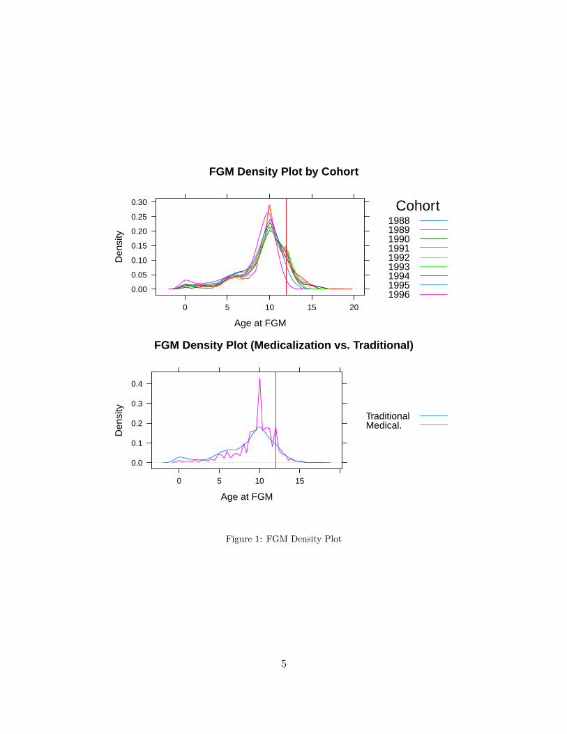
FGM Density Plot by Cohort

Age at FGM

Den

sity

0.00

0.05

0.10

0.15

0.20

0.25

0.30

0 5 10 15 20

Cohort198819891990199119921993199419951996

FGM Density Plot (Medicalization vs. Traditional)

Age at FGM

Den

sity

0.0

0.1

0.2

0.3

0.4

0 5 10 15

TraditionalMedical.

Figure 1: FGM Density Plot

5

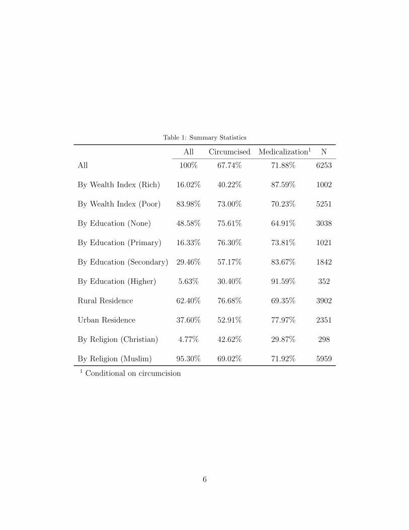
Table 1: Summary Statistics

All Circumcised Medicalization1 N

All 100% 67.74% 71.88% 6253

By Wealth Index (Rich) 16.02% 40.22% 87.59% 1002

By Wealth Index (Poor) 83.98% 73.00% 70.23% 5251

By Education (None) 48.58% 75.61% 64.91% 3038

By Education (Primary) 16.33% 76.30% 73.81% 1021

By Education (Secondary) 29.46% 57.17% 83.67% 1842

By Education (Higher) 5.63% 30.40% 91.59% 352

Rural Residence 62.40% 76.68% 69.35% 3902

Urban Residence 37.60% 52.91% 77.97% 2351

By Religion (Christian) 4.77% 42.62% 29.87% 298

By Religion (Muslim) 95.30% 69.02% 71.92% 5959

1 Conditional on circumcision

6

Proportion of FGM

Cohort

Fre

quen

cy

0.0

0.2

0.4

0.6

0.8

1.0

1988 1989 1990 1991 1992 1993 1994 1995 1996

Yes No

Proportion of Medicalization

Cohort

Fre

quen

cy

0.0

0.2

0.4

0.6

0.8

1.0

1988 1989 1990 1991 1992 1993 1994 1995 1996

Yes No

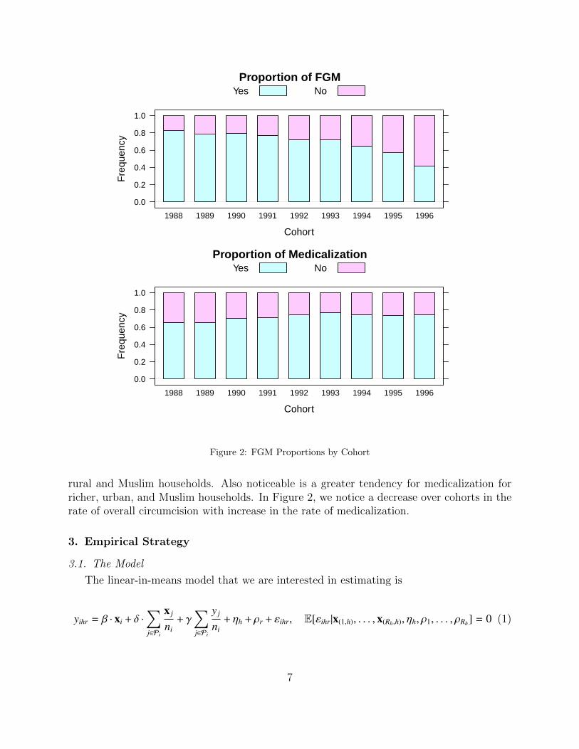
Figure 2: FGM Proportions by Cohort

rural and Muslim households. Also noticeable is a greater tendency for medicalization forricher, urban, and Muslim households. In Figure 2, we notice a decrease over cohorts in therate of overall circumcision with increase in the rate of medicalization.

3. Empirical Strategy

3.1. The Model

The linear-in-means model that we are interested in estimating is

yihr = β · xi + δ ·∑j∈Pi

x j

ni+ γ∑j∈Pi

y j

ni+ ηh + ρr + εihr, E[εihr|x(1,h), . . . , x(Rh,h), ηh, ρ1, . . . , ρRh] = 0 (1)

7

Table 2: Governorate Summary Statistics

Cir

cum

cize

d

Med

icaliza

tion

Wea

lth

Ind

ex(R

ich)

Ru

ral

Res

iden

ce

Rel

igio

n(C

hri

stia

n)

Moth

erC

ircu

mci

zed

Moth

er’s

Mari

tal

Age

Age

of

Cir

cum

cisi

on

N

All 67.7% 48.7% 16.0% 62.4% 4.8% 96.0% 18.5 (3.8) 9.2 (2.8) 6253Alexandria 38.0% 32.2% 47.3% 0.0% 4.4% 90.7% 20.6 (4.0) 10.4 (2.0) 205Assuit 78.1% 31.0% 6.6% 72.0% 11.6% 97.0% 17.6 (3.3) 8.1 (2.4) 439Aswan 97.8% 70.2% 12.4% 70.8% 3.4% 100.0% 17.2 (3.9) 5.7 (2.3) 178Behera 46.1% 35.5% 10.3% 81.9% 0.9% 97.5% 18.5 (3.6) 10.8 (2.0) 321Beni Suef 79.1% 59.9% 6.4% 86.6% 2.2% 100.0% 17.5 (3.5) 10.9 (1.8) 359Cairo 48.3% 33.0% 45.8% 0.0% 5.9% 96.9% 20.1 (4.2) 9.6 (2.0) 321Dakahlia 56.6% 41.4% 12.1% 69.0% 0.3% 96.9% 18.8 (3.7) 10.5 (2.2) 290Damietta 25.6% 21.8% 40.6% 57.1% 0.0% 95.5% 19.7 (3.9) 10.9 (2.1) 133Fayoum 57.7% 24.4% 2.7% 84.9% 1.4% 99.3% 16.7 (2.9) 11.2 (1.7) 291Gharbia 70.6% 53.3% 15.4% 73.5% 0.4% 96.7% 19.9 (3.7) 9.9 (1.7) 272Giza 65.6% 57.5% 32.6% 39.2% 5.1% 96.0% 18.5 (4.0) 10.4 (1.5) 273Ismailia 82.9% 73.0% 15.8% 51.3% 0.0% 100.0% 19.2 (3.3) 10.6 (1.6) 152Kafr El Sheikh 74.7% 66.2% 4.4% 73.3% 0.9% 99.6% 19.1 (3.8) 10.7 (1.3) 225Kalyubia 78.5% 74.7% 18.8% 58.6% 7.3% 100.0% 19.3 (3.7) 9.5 (1.0) 261Matrouh 9.9% 6.1% 7.6% 42.7% 0.0% 26.0% 17.5 (3.7) 10.2 (1.7) 131Menoufia 82.5% 66.7% 7.7% 76.5% 3.4% 98.3% 19.3 (3.8) 9.9 (1.6) 234Menya 60.3% 39.4% 5.6% 85.1% 12.3% 94.2% 16.9 (3.4) 10.5 (1.7) 464New Valley 82.2% 54.8% 24.7% 42.5% 0.0% 100.0% 20.3 (4.3) 9.5 (2.4) 73North Sinai 42.6% 16.7% 15.7% 41.7% 0.0% 83.3% 19.3 (3.6) 10.9 (1.5) 108Port Said 15.6% 7.3% 79.8% 0.0% 0.9% 95.4% 22.2 (3.5) 10.6 (2.7) 109Qena 93.7% 75.5% 10.3% 71.6% 6.3% 99.1% 17.2 (3.6) 5.8 (3.5) 458Red Sea 89.6% 81.2% 20.8% 0.0% 18.8% 100.0% 18.2 (3.9) 8.3 (1.9) 48Sharkia 79.3% 65.0% 4.5% 89.2% 1.6% 100.0% 18.2 (3.0) 10.5 (1.3) 314Souhag 89.9% 53.7% 7.0% 81.9% 11.8% 99.5% 17.7 (3.4) 7.4 (3.3) 415South Sinai 68.0% 40.0% 48.0% 24.0% 8.0% 100.0% 19.0 (4.2) 9.9 (1.4) 25Suez 63.6% 46.1% 33.8% 0.0% 0.6% 98.1% 21.0 (3.9) 10.3 (1.7) 154

1 Standard deviation is reported between parenthesis

8

The subscript i = {1, . . . ,N} identifies daughters (the observations of interest), h ={1, . . . ,M} their household, and r = {1, . . . ,Rh} their order of birth within their household,where Rh is the number of daughters in household h. The variable yihr is a indicator ofwhether a particular daughter has undergone FGM. Each daughter i has a peer group whosecharacteristics and behavior might influence i’s household’s FGM decision. In this specifica-tion, we model it as the set observations Pi (ni = |Pi| is the number of i’s neighbors). Thedependent variable is regressed on

• The K × 1 vector xi of a daughter’s individual characteristics, composed of daughter-specific regressors and household-invariant regressors

• The mean of x of a daughter’s peer group Pi, and whose K × 1 vector of coefficients, δ,represents exogenous social effects

• The mean of y of a daughter’s peer group Pi, and whose coefficient, γ, representsendogenous social effects

• The household fixed effect ηh

• The birth order fixed effect ρr

We transform this model to use matrix notation to facilitate the use of an interactionmatrix to represent peer groups (Bramoulle et al., 2009). We use the logical N × N matrix

W to indicate whether any two daughters are considered peers (we will further explain whatdefines peers for the purposes of this model below).

(Wij) = 1{i and j are peers}

We further normalize this matrix to the row stochastic W, where

(Wij) =Wij

ni

Our model now becomes

y = Xβ +WXδ +Wyγ + η + ρ + ε (2)

where y is N×1 vector of FGM status, X is a N×K matrix of daughters’ characteristics, ηis a N×1 vector of {η1, . . . , ηM}, each repeated Rh times, and ρ is a N×1 vector of {ρ1, . . . , ρRh}.

3.1.1. Reference Group

In order to carry out our social effects analysis we need to define each daughter’s peergroup Pi or the interaction matrix W. First we define the logical matrices

9

A : (Aij) = 1{disti j ≤ 10 kilometers5}

C : (Cij) = 1{|agei − age j| ≤ 1 year}

H : (Cij) = 1{householdi = household j}

from which we define the interaction matrix, excluding all same household daughtersfrom the peer group, since we are ultimately interested in estimating the influence of peerson a household’s decision making.

W = A ◦ C ◦ ¬H

This means we define the peer group that would influence a household’s FGM decision fordaughter i as all daughters i) not in the same household, ii) who are within a ten kilometerradius, iii) and whose absolute age difference does not exceed one year.

While we do model the peer groups or ‘neighborhoods’ as a network (as is commonly donein the social networks literature), we do not mean to model explicit social links betweenhouseholds or daughters. A daughter’s peer group is used to estimate what is commonpractice in the area of residence6. In other words, we decide to consider two daughters asnetwork neighbors if all the conditions outlined above are true. It might be more intuitiveto understand how this is modeled by viewing the space of observations as divided intoplanes, with each plane representing a cohort group, and on each plane, observations of thatcohort group are placed according to their GPS coordinates. On each plane we then haveoverlapping circles, each centered on an observation (or more accurately, its cluster), and anyobservation within such a circle is considered a neighbor, which we represent by a networklink. Figure 3 shows an example of such a network.

3.1.2. Identification

So far, this is a typical linear-in-means model with all the identification challenges thisentails: simultaneity (the reflection problem), endogeneity, and correlated effects (Manski,1993; Moffitt, 2001; Blume et al., 2010; Bramoulle et al., 2009). The reduced form of thismodel would be

y = (I −Wγ)−1Xβ + (I −Wγ)−1WXδ + (I −Wγ)−1η + (I −Wγ)−1ρ + (I −Wγ)−1ε (3)

5Any smaller range would be problematic according to the DHS because of location displacement, wherebyGPS coordinates are randomly altered in order to preserve survey subjects’ privacy. This is also the reasonwe do not rely on the distance between clusters to weigh our interaction matrix (DHS, 2012).

6Inference based on such estimated averages is further discussed below.

10

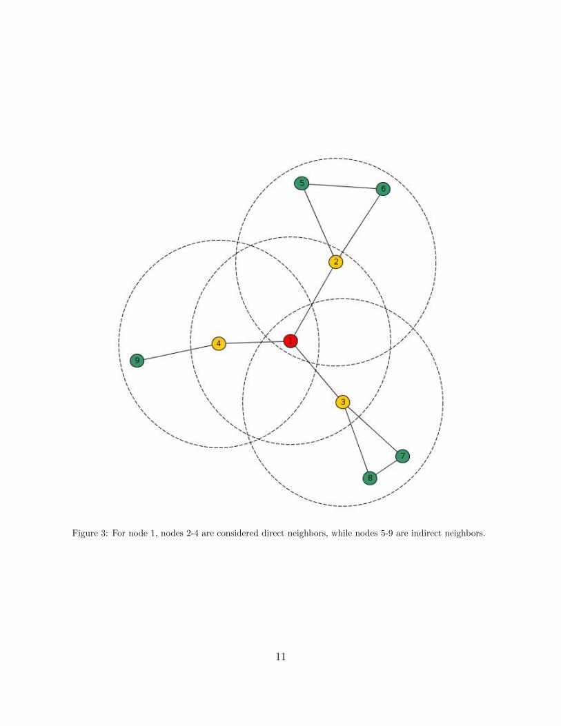
Figure 3: For node 1, nodes 2-4 are considered direct neighbors, while nodes 5-9 are indirect neighbors.

11

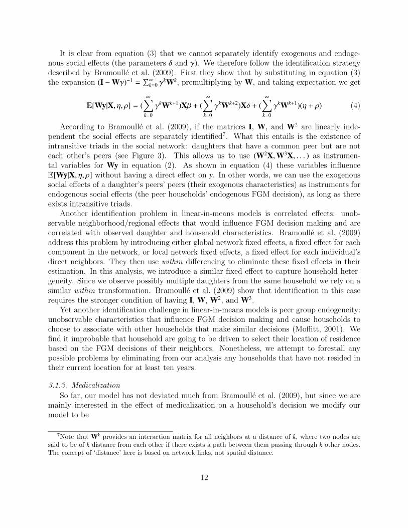
It is clear from equation (3) that we cannot separately identify exogenous and endoge-nous social effects (the parameters δ and γ). We therefore follow the identification strategydescribed by Bramoulle et al. (2009). First they show that by substituting in equation (3)the expansion (I −Wγ)−1 =

∑∞k=0 γ

kWk, premultiplying by W, and taking expectation we get

E[Wy|X, η, ρ] = (∞∑

k=0

γkWk+1)Xβ + (∞∑

k=0

γkWk+2)Xδ + (∞∑

k=0

γkWk+1)(η + ρ) (4)

According to Bramoulle et al. (2009), if the matrices I, W, and W2 are linearly inde-pendent the social effects are separately identified7. What this entails is the existence ofintransitive triads in the social network: daughters that have a common peer but are noteach other’s peers (see Figure 3). This allows us to use (W2X,W3X, . . . ) as instrumen-tal variables for Wy in equation (2). As shown in equation (4) these variables influenceE[Wy|X, η, ρ] without having a direct effect on y. In other words, we can use the exogenoussocial effects of a daughter’s peers’ peers (their exogenous characteristics) as instruments forendogenous social effects (the peer households’ endogenous FGM decision), as long as thereexists intransitive triads.

Another identification problem in linear-in-means models is correlated effects: unob-servable neighborhood/regional effects that would influence FGM decision making and arecorrelated with observed daughter and household characteristics. Bramoulle et al. (2009)address this problem by introducing either global network fixed effects, a fixed effect for eachcomponent in the network, or local network fixed effects, a fixed effect for each individual’sdirect neighbors. They then use within differencing to eliminate these fixed effects in theirestimation. In this analysis, we introduce a similar fixed effect to capture household heter-geneity. Since we observe possibly multiple daughters from the same household we rely on asimilar within transformation. Bramoulle et al. (2009) show that identification in this caserequires the stronger condition of having I, W, W2, and W3.

Yet another identification challenge in linear-in-means models is peer group endogeneity:unobservable characteristics that influence FGM decision making and cause households tochoose to associate with other households that make similar decisions (Moffitt, 2001). Wefind it improbable that household are going to be driven to select their location of residencebased on the FGM decisions of their neighbors. Nonetheless, we attempt to forestall anypossible problems by eliminating from our analysis any households that have not resided intheir current location for at least ten years.

3.1.3. Medicalization

So far, our model has not deviated much from Bramoulle et al. (2009), but since we aremainly interested in the effect of medicalization on a household’s decision we modify ourmodel to be

7Note that Wk provides an interaction matrix for all neighbors at a distance of k, where two nodes aresaid to be of k distance from each other if there exists a path between them passing through k other nodes.The concept of ‘distance’ here is based on network links, not spatial distance.

12

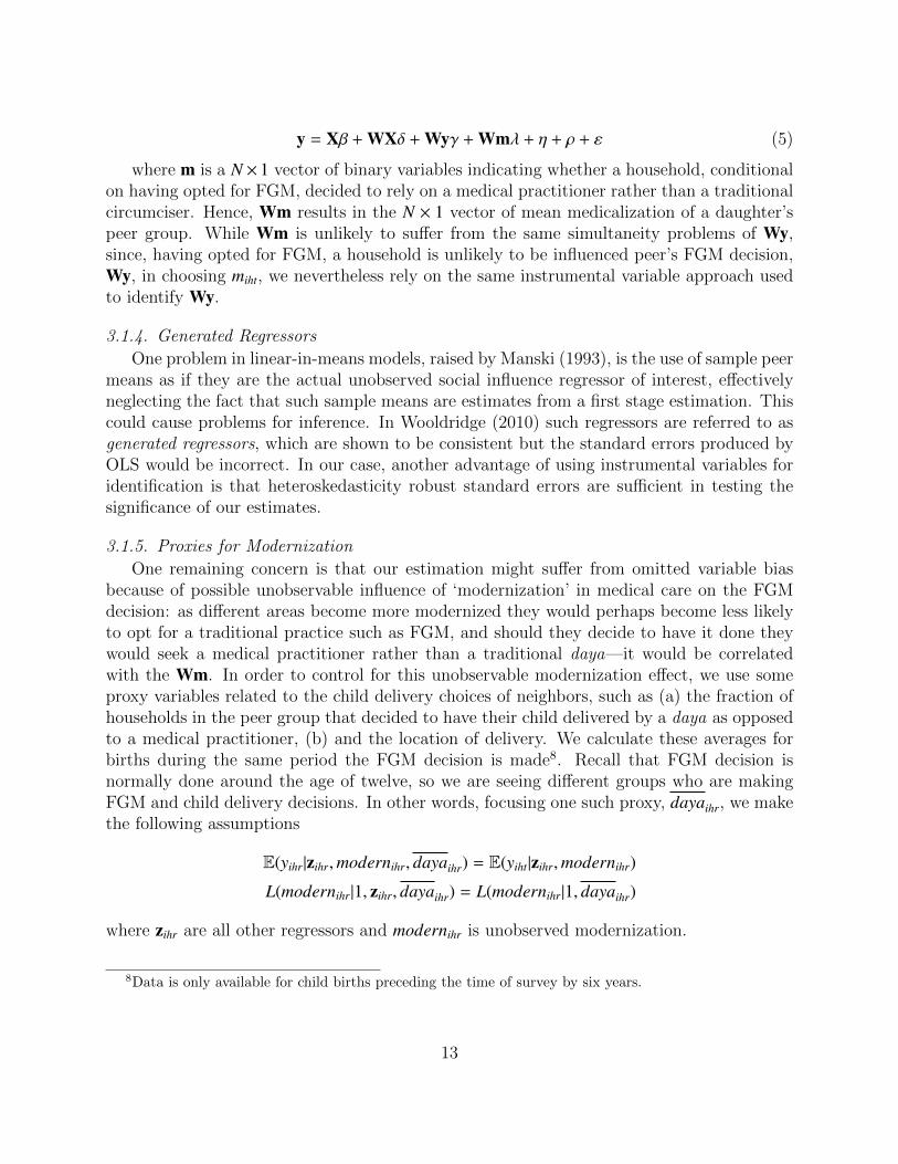
y = Xβ +WXδ +Wyγ +Wmλ + η + ρ + ε (5)

where m is a N ×1 vector of binary variables indicating whether a household, conditionalon having opted for FGM, decided to rely on a medical practitioner rather than a traditionalcircumciser. Hence, Wm results in the N × 1 vector of mean medicalization of a daughter’speer group. While Wm is unlikely to suffer from the same simultaneity problems of Wy,since, having opted for FGM, a household is unlikely to be influenced peer’s FGM decision,Wy, in choosing miht, we nevertheless rely on the same instrumental variable approach usedto identify Wy.

3.1.4. Generated Regressors

One problem in linear-in-means models, raised by Manski (1993), is the use of sample peermeans as if they are the actual unobserved social influence regressor of interest, effectivelyneglecting the fact that such sample means are estimates from a first stage estimation. Thiscould cause problems for inference. In Wooldridge (2010) such regressors are referred to asgenerated regressors, which are shown to be consistent but the standard errors produced byOLS would be incorrect. In our case, another advantage of using instrumental variables foridentification is that heteroskedasticity robust standard errors are sufficient in testing thesignificance of our estimates.

3.1.5. Proxies for Modernization

One remaining concern is that our estimation might suffer from omitted variable biasbecause of possible unobservable influence of ‘modernization’ in medical care on the FGMdecision: as different areas become more modernized they would perhaps become less likelyto opt for a traditional practice such as FGM, and should they decide to have it done theywould seek a medical practitioner rather than a traditional daya—it would be correlatedwith the Wm. In order to control for this unobservable modernization effect, we use someproxy variables related to the child delivery choices of neighbors, such as (a) the fraction ofhouseholds in the peer group that decided to have their child delivered by a daya as opposedto a medical practitioner, (b) and the location of delivery. We calculate these averages forbirths during the same period the FGM decision is made8. Recall that FGM decision isnormally done around the age of twelve, so we are seeing different groups who are makingFGM and child delivery decisions. In other words, focusing one such proxy, dayaihr, we makethe following assumptions

E(yihr|zihr,modernihr, dayaihr) = E(yiht|zihr,modernihr)

L(modernihr|1, zihr, dayaihr) = L(modernihr|1, dayaihr)

where zihr are all other regressors and modernihr is unobserved modernization.

8Data is only available for child births preceding the time of survey by six years.

13

3.2. Implementation

3.2.1. Variables

Of the household characteristics we are interested in we use:

• Wealth level: ‘poor’ or ‘rich’, with ‘poor’ as the omitted level9

• Urban or rural residence, with rural residence as the omitted level

• The mother’s marital age

• The mother’s FGM status

• Religion: Christian or Muslim, with Muslim as the omitted level

• The sex of the head of household, with male as the omitted level

• Whether seeking medical help is ‘not a problem’ or a ‘big problem’ due to distance orcost, with ‘not a problem’ as the omitted level

• Highest level of mother’s education: no education, primary education, secondary edu-cation, or higher education, with no education as the omitted level

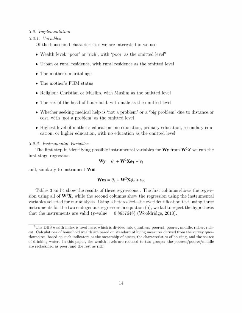
3.2.2. Instrumental Variables

The first step in identifying possible instrumental variables for Wy from W2X we run thefirst stage regression

Wy = θ1 +W2Xφ1 + ν1

and, similarly to instrument Wm

Wm = θ2 +W2Xφ2 + ν2.

Tables 3 and 4 show the results of these regressions . The first columns shows the regres-sion using all of W2X, while the second columns show the regression using the instrumentalvariables selected for our analysis. Using a heteroskedastic overidentification test, using threeinstruments for the two endogenous regressors in equation (5), we fail to reject the hypothesisthat the instruments are valid (p-value = 0.8657648) (Wooldridge, 2010).

9The DHS wealth index is used here, which is divided into quintiles: poorest, poorer, middle, richer, rich-est. Calculations of household wealth are based on standard of living measures derived from the survey ques-tionnaires, based on such indicators as the ownership of assets, the characteristics of housing, and the sourceof drinking water. In this paper, the wealth levels are reduced to two groups: the poorest/poorer/middleare reclassified as poor, and the rest as rich.

14

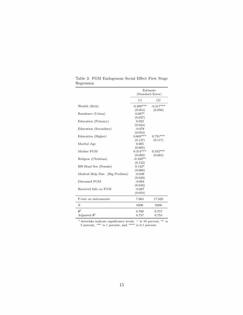
Table 3: FGM Endogenous Social Effect First StageRegression

Estimate(Standard Error)

(1) (2)

Wealth (Rich) -0.208*** -0.217***(0.054) (0.050)

Residence (Urban) 0.087*(0.037)

Education (Primary) 0.022(0.044)

Education (Secondary) -0.078(0.054)

Education (Higher) 0.603*** 0.731***(0.127) (0.117)

Marital Age 0.005(0.005)

Mother FGM 0.314*** 0.352***(0.092) (0.084)

Religion (Christian) -0.320**(0.122)

HH Head Sex (Female) 0.142*(0.066)

Medical Help Dist. (Big Problem) -0.038(0.049)

Discussed FGM -0.004(0.040)

Received Info on FGM -0.007(0.054)

F-test on instruments 7.664 17.629

N 6206 6206

R2 0.760 0.757Adjusted R2 0.757 0.754

1 Asterisks indicate significance levels: ‘·’ is 10 percent, ‘*’ is5 percent, ‘**’ is 1 percent, and ‘***’ is 0.1 percent.

15

Table 4: Medicalization Endogenous Social EffectFirst Stage Regression

Estimate(Standard Error)

(1) (2)

Wealth (Rich) -0.263***(0.073)

Residence (Urban) -0.018(0.052)

Education (Primary) 0.025(0.071)

Education (Secondary) -0.034(0.063)

Education (Higher) 0.372**(0.141)

Marital Age 0.015**(0.006)

Mother FGM 0.149·(0.083)

Religion (Christian) -0.426*** -0.444***(0.111) (0.108)

HH Head Sex (Female) 0.122(0.095)

Medical Help Dist. (Big Problem) 0.041(0.061)

Discussed FGM 0.023(0.050)

Received Info on FGM -0.084*(0.035)

F-test on instruments 5.659 17.006

N 6206 6206

R2 0.608 0.601Adjusted R2 0.603 0.597

1 Asterisks indicate significance levels: ‘·’ is 10 percent, ‘*’ is5 percent, ‘**’ is 1 percent, and ‘***’ is 0.1 percent.

16

4. Results

4.1. Direct Effects

The first regression results presented are those for direct effects of individual character-istics on the likelihood of FGM only (shown in Table 5); we want to examine how particularobservable characteristics of households influence the FGM decision for their daughters. Thefirst column shows the results using an OLS regression while the second is shown for ahousehold fixed effects (FE) regression.

The first thing to observe is the apparent increased likelihood of FGM, in the FE results,for daughters of the fifth or sixth birth order. We also notice, in both estimations, a significantnegative likelihood of FGM for younger cohorts, suggesting a decreasing FGM trend acrossthe country over time. In the OLS regression, we see some expected results: a significantnegative likelihood of FGM for wealthier households, households that reside in urban areas,households where mothers got married at an older age, households that discussed FGMwith their neighbors, and households where mothers have higher levels of education; anda significant positive likelihood for households with more daughters. A significant negativelikelihood is also found for Christian households (compared to Muslim households), which issomewhat surprising considering that FGM is a practice that predates Islam in Egypt.

4.2. Social Effects

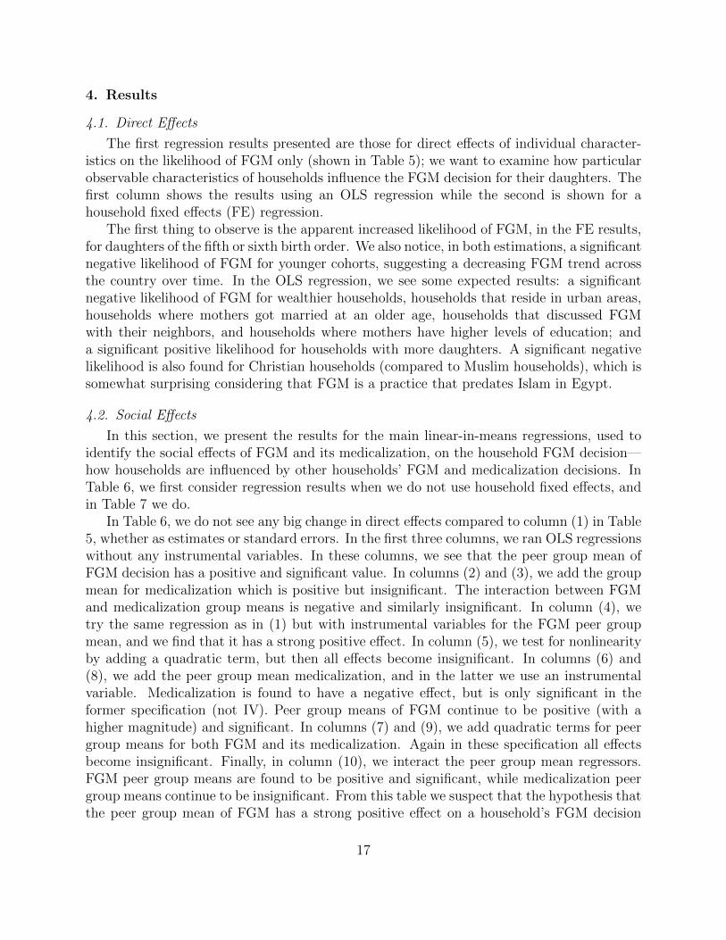
In this section, we present the results for the main linear-in-means regressions, used toidentify the social effects of FGM and its medicalization, on the household FGM decision—how households are influenced by other households’ FGM and medicalization decisions. InTable 6, we first consider regression results when we do not use household fixed effects, andin Table 7 we do.

In Table 6, we do not see any big change in direct effects compared to column (1) in Table5, whether as estimates or standard errors. In the first three columns, we ran OLS regressionswithout any instrumental variables. In these columns, we see that the peer group mean ofFGM decision has a positive and significant value. In columns (2) and (3), we add the groupmean for medicalization which is positive but insignificant. The interaction between FGMand medicalization group means is negative and similarly insignificant. In column (4), wetry the same regression as in (1) but with instrumental variables for the FGM peer groupmean, and we find that it has a strong positive effect. In column (5), we test for nonlinearityby adding a quadratic term, but then all effects become insignificant. In columns (6) and(8), we add the peer group mean medicalization, and in the latter we use an instrumentalvariable. Medicalization is found to have a negative effect, but is only significant in theformer specification (not IV). Peer group means of FGM continue to be positive (with ahigher magnitude) and significant. In columns (7) and (9), we add quadratic terms for peergroup means for both FGM and its medicalization. Again in these specification all effectsbecome insignificant. Finally, in column (10), we interact the peer group mean regressors.FGM peer group means are found to be positive and significant, while medicalization peergroup means continue to be insignificant. From this table we suspect that the hypothesis thatthe peer group mean of FGM has a strong positive effect on a household’s FGM decision

17

Table 5: Direct Effects Only

Estimate(Standard Error)

(1) (2)OLS FE

Birth Order2 0.012 -0.001

(0.012) (0.018)3 -0.008 -0.039

(0.027) (0.036)4 -0.125* -0.067

(0.060) (0.070)5 0.109 0.151*

(0.102) (0.060)6 0.069 0.229***

(0.052) (0.060)Cohort1989 -0.014 -0.009

(0.021) (0.025)1990 -0.005 0.009

(0.020) (0.024)1991 -0.043* -0.040

(0.020) (0.029)1992 -0.063** -0.038

(0.021) (0.032)1993 -0.071** -0.072*

(0.022) (0.036)1994 -0.149*** -0.120**

(0.024) (0.040)1995 -0.208*** -0.206***

(0.025) (0.046)1996 -0.372*** -0.319***

(0.024) (0.051)Wealth (Rich) -0.094***

(0.023)Residence (Urban) -0.083***

(0.016)Marital Age -0.005**

(0.002)Mother FGM 0.334***

(0.029)Religion (Christian) -0.274***

(0.032)HH Head Sex (Female) -0.021

(0.018)Medical Help Dist. (Big Problem) -0.004

(0.014)Medical Help Cost (Big Problem) -0.007

(0.013)Discussed FGM -0.031*

(0.013)Received Info on FGM 0.005

(0.014)Number of Daughters 0.032***

(0.008)Education LevelPrimary 0.009

(0.015)Secondary -0.079***

(0.016)Higher -0.192***

(0.035)

N 6206 6253

R2 0.357 0.191

Adjusted R2 0.352 0.056

1 Asterisks indicate significance levels: ‘·’ is 10 percent, ‘*’ is 5percent, ‘**’ is 1 percent, and ‘***’ is 0.1 percent.

2 In the OLS regression, fixed effects for governorates were alsoused.

18

is probably true, but we are unable to make any clear conclusions about medicalization.However, as stated above, because of the problem with correlated effects and the possibleendogeneity due to unobservable household effects that are correlated with our regressors,we need to leverage the within information we have about households.

In Table 7, we introduce household fixed effects to address some of these problems,coupled with the existing instrumental variable strategy. In columns (1) and (2), we regressonly on the peer group means of FGM and we continue to find a significant positive effect,with some convexity on introducing a quadratic term. In columns (3) and (4), we introducemedicalization, and in the latter specification we use instrumental variables. We now observea significant negative effect (almost halved in the latter specification). The effect of peergroup FGM means continues to be significantly positive and increases in magnitude. Incolumns (5) and (6), we introduced some nonlinearity. In column (5), there is still a positiveand negative effect to peer group means of FGM and medicalization, respectively—with someconcavity and convexity, respectively. In column (6), the significance and direction of effectis unchanged, but the magnitudes are diminished (in this specification we see the highestlevel of R2 in this table). There does appear to be a reduced negative effect of medicalizationas FGM peer group means increase, but is only significant at the 10% level.

19

Table 6: FGM Endogenous Effects Regression (Pooled)

Estimate(Standard Error)

(1) (2) (3) (4) (5) (6) (7) (8) (9) (10)OLS OLS OLS 2SLS 2SLS 2SLS 2SLS 2SLS 2SLS 2SLS

Wealth (Rich) -0.083*** -0.083*** -0.082*** -0.073** -0.072** -0.076** -0.077** -0.076** -0.073** -0.073**(0.023) (0.023) (0.023) (0.024) (0.024) (0.024) (0.024) (0.024) (0.024) (0.024)

Residence (Urban) -0.081*** -0.081*** -0.081*** -0.081*** -0.079*** -0.086*** -0.085*** -0.087*** -0.082*** -0.084***(0.017) (0.017) (0.017) (0.017) (0.017) (0.018) (0.018) (0.019) (0.018) (0.017)

Marital Age -0.005** -0.005** -0.005** -0.006*** -0.006*** -0.006*** -0.006*** -0.006*** -0.006*** -0.006***(0.002) (0.002) (0.002) (0.002) (0.002) (0.002) (0.002) (0.002) (0.002) (0.002)

Mother FGM 0.301*** 0.302*** 0.301*** 0.276*** 0.276*** 0.267*** 0.274*** 0.265*** 0.275*** 0.273***(0.031) (0.031) (0.031) (0.036) (0.036) (0.039) (0.037) (0.039) (0.037) (0.038)

Religion (Christian) -0.266*** -0.266*** -0.266*** -0.259*** -0.257*** -0.261*** -0.255*** -0.261*** -0.256*** -0.259***(0.031) (0.031) (0.031) (0.031) (0.031) (0.031) (0.031) (0.031) (0.031) (0.031)

HH Head Sex (Female) -0.018 -0.018 -0.018 -0.018 -0.019 -0.014 -0.018 -0.014 -0.019 -0.017(0.018) (0.018) (0.018) (0.018) (0.018) (0.019) (0.019) (0.019) (0.019) (0.018)

Medical Help Distance (Big Problem) -0.003 -0.003 -0.003 -0.002 -0.001 -0.002 0.000 -0.002 -0.001 -0.002(0.014) (0.014) (0.014) (0.014) (0.014) (0.015) (0.015) (0.015) (0.014) (0.014)

Medical Help Cost (Big Problem) -0.005 -0.006 -0.006 -0.004 -0.003 0.001 0.002 0.002 -0.002 -0.005(0.012) (0.012) (0.012) (0.013) (0.013) (0.013) (0.013) (0.014) (0.013) (0.013)

Discussed FGM -0.029* -0.029* -0.029* -0.027* -0.026· -0.028* -0.027* -0.028* -0.027* -0.028*(0.013) (0.013) (0.013) (0.013) (0.013) (0.013) (0.014) (0.014) (0.013) (0.013)

Received Info on FGM 0.008 0.008 0.008 0.012 0.012 0.014 0.012 0.015 0.012 0.013(0.014) (0.014) (0.014) (0.014) (0.014) (0.015) (0.015) (0.015) (0.015) (0.015)

Number of Daughters 0.034*** 0.034*** 0.034*** 0.034*** 0.032*** 0.032*** 0.026** 0.032*** 0.030** 0.035***(0.009) (0.009) (0.009) (0.009) (0.009) (0.009) (0.010) (0.009) (0.010) (0.009)

Education LevelPrimary 0.009 0.009 0.009 0.009 0.010 0.011 0.016 0.012 0.012 0.009

(0.015) (0.015) (0.015) (0.015) (0.015) (0.016) (0.016) (0.016) (0.016) (0.015)Secondary -0.076*** -0.076*** -0.076*** -0.073*** -0.074*** -0.070*** -0.070*** -0.069*** -0.072*** -0.070***

(0.016) (0.016) (0.016) (0.017) (0.017) (0.017) (0.017) (0.018) (0.017) (0.017)Higher -0.204*** -0.204*** -0.204*** -0.215*** -0.215*** -0.216*** -0.209*** -0.216*** -0.213*** -0.215***

(0.034) (0.034) (0.034) (0.034) (0.034) (0.034) (0.034) (0.035) (0.035) (0.034)

f gm jt 0.526*** 0.505*** 0.521*** 1.065*** 0.625 1.538*** -0.001 1.641** 0.399 1.278***(0.040) (0.046) (0.049) (0.238) (0.437) (0.406) (0.663) (0.532) (0.730) (0.350)

( f gm jt)2 0.414 1.143* 0.642

(0.358) (0.531) (0.581)

med jt 0.028 0.119 -0.547* 0.040 -0.672 0.182 0.534(0.035) (0.101) (0.230) (0.420) (0.575) (1.036) (0.897)

(med jt)2 -0.469 -0.289(0.328) (0.827)

f gm jt × med jt -0.101 -0.717(0.101) (0.944)

N 6206 6206 6206 6206 6206 6206 6206 6206 6206 6206

R2 0.387 0.387 0.388 0.361 0.354 0.332 0.335 0.319 0.355 0.354Adjusted R2 0.380 0.380 0.380 0.354 0.347 0.324 0.327 0.311 0.347 0.346

1 Asterisks indicate significance levels: ‘·’ is 10 percent, ‘*’ is 5 percent, ‘**’ is 1 percent, and ‘***’ is 0.1 percent.2 Other regressors not shown: governorate fixed effects, cohort (year of birth) fixed effects, order of birth fixed effects, ‘modernization’ proxy variables, and peer group

means of exogenous household characteristics (exogenous social effects).

20

Table 7: FGM Endogenous Effects Regression (Household Fixed Effects)

Estimate(Standard Error)

(1) (2) (3) (4) (5) (6) (7) (8)

f gm jt 1.180*** -0.964*** 1.328*** 1.299*** 1.281*** 0.917*** 1.849*** 1.939***(0.081) (0.184) (0.095) (0.094) (0.238) (0.088) (0.120) (0.126)

( f gm jt)2 1.410*** -0.433*

(0.145) (0.173)

med jt -0.592*** -0.265*** -2.151*** -0.493** -0.472*** -1.298***(0.073) (0.066) (0.246) (0.166) (0.096) (0.139)

(med jt)2 1.645***(0.198)

f gm jt × med jt 0.265·(0.158)

med jt× Urban -0.125 0.207(0.155) (0.181)

med jt× Medical Help Distance -0.224·(0.131)

med jt× Urban × Medical Help Distance 1.856***(0.489)

med jt× Medical Help Cost 0.644***(0.140)

med jt× Urban × Medical Help Cost 1.189***(0.328)

N 6229 6229 6229 6229 6229 6229 6229 6229

R2 0.185 0.171 0.195 0.191 0.161 0.213 0.145 0.132Adjusted R2 0.054 0.050 0.057 0.056 0.047 0.062 0.042 0.038

1 Asterisks indicate significance levels: ‘·’ is 10 percent, ‘*’ is 5 percent, ‘**’ is 1 percent, and ‘***’ is 0.1 percent.2 Other regressors not shown: governorate fixed effects, cohort (year of birth) fixed effects, order of birth fixed effects, ‘modernization’ proxy

variables, and peer group means of exogenous household characteristics (exogenous social effects).

21

Table 8: Urban/Rural and Medical Help Interactions

Estimate(p-value)

Rural Urban

Medical Help Distance (No Problem) -0.472*** -0.597***(0.000) (0.000)

Medical Help Distance (Problem) -0.696*** 1.034*(0.000) (0.024)

Difference 0.224· -1.631***(0.086) (0.001)

Medical Help Cost (No Problem) -1.298*** -1.091***(0.000) (0.000)

Medical Help Cost (Problem) -0.655*** 0.741**(0.000) (0.006)

Difference -0.644*** -1.832***(0.000) (0.000)

1 Asterisks indicate significance levels: ‘·’ is 10 percent, ‘*’ is5 percent, ‘**’ is 1 percent, and ‘***’ is 0.1 percent.

Having established that there is a negative effect to medicalization, we introduce someinteraction terms in the last two columns of Table 7 to further investigate how the effectmight vary in different contexts, namely, urban versus rural, and with different levels ofdifficulty accessing medical help (either because of distance or cost). With three levels ofinteractions, it is easier to analyze our results by using Table 8. We see that in rural areasmedicalization has a negative effect, does not seem to be affected by difficulty in accessingmedical help due to distance, and does seem to have a weaker negative effect if the householdhas difficulty accessing medical help due to cost. In urban areas, the effect of medicalizationis more nuanced; it appears to be negative for households with no problem accessing medicalhelp (for either of the reasons considered), but has significant positive effect if they do haveproblems accessing medical help.

5. Conclusion

As has been shown by our results, there is a strong social component, in Egypt, tohouseholds’ decision to circumcise their daughters. Households tended to follow the samebehavior as other members of their community. However, in terms of medicalization, thereappears to be a negative social effect (for most households with no problems accessing medicalhelp). Households were less likely to choose FGM for their daughters the more prevalent ismedicalization in their peer group. This appears to strengthens the harm reduction argument

22

of those who call for tolerating medicalization in the interest of providing a less painful andsanitary procedure for those who opt for FGM (Shell-Duncan, 2001). These results are also acall on policy makers who are seeking to eliminate FGM, to consider the possible unintendedconsequences of focusing on eliminating medicalization in government clinics. Our resultspoint to directly influencing households’ FGM decision as a possibly more fruitful policy, sincewe see a strong multiplier effect, since households have a very strong endogenous influenceon each other. This could be done by increasing awareness in communities of the harmfulnature of this practice as was carried out in Senegal (Diop and Askew, 2009), while notpushing them away from medical clinics back into the domain of traditional circumcisers,where they might be less accessible to outreach campaigns.

One proposed story explaining these findings, is related to the pernicious nature of themarriage market social network in which dayas might play the role of ‘quality certifiers’. Dueto the unobservable and unverifiable nature of FGM, reputation plays a critical role here.As the FGM procedure moves away from the traditional sphere into that of professionalhealthcare its links to the marriage market is weakened, as healthcare providers are lesslikely to play a role in the marriage market. We might also be observing a modernizationscenario, in which the endogenous social effect of medicalization is a proxy for a move awayfrom traditional practices across all households in a particular area, irrespective of the otherobserved household characteristics. As mentioned, we attempt to address this problem bythe use of data on child delivery choices contemporary to the FGM decision.

However, we must be cautious in making any recommendations calling for a rollbackin the elimination for FGM in medical facilities. There is always the danger that such areversal of policy might give the impression of greater legitimacy, and households that werepreviously indecisive about FGM would regard such a move as approving of the procedure.In fact, some of our results should make us very cautious in dealing with the problem oflegitimization. We see a positive effect to medicalization in urban areas with poor accessto medical help (either due to distance or cost), which could plausibly be the influence ofobserving increased medicalization in one’s peer group and perceiving it as evidence of itsbenefit, and without easy access to medical practitioners (and their mitigating influence)FGM is increasingly sought from traditional circumcisers10.

Acknowledgments

Special thanks to Randall Ellis, Robert E.B. Lucas, Dilip Mookherjee, Wesley Yin, Ke-hinde Ajayi, Julian TszKin Chan, and Giulia La Mattina for their advice and suggestions.I’m also grateful to Emily Gee and Marcella Bombardieri for reviewing this paper and sug-gesting corrections.

10Similar fears were raised in response to Indonesia’s Ministry of Health publishing guidelines for conduc-tion FGM (Ind, 2011)

23

References

Demographic and Health Survey Phase III Sampling Manual, 1996. URLhttp://www.measuredhs.com/pubs/pdf/DHSM4/DHS_III_Sampling_Manual.pdf.

INDONESIA: FGM/C regulations mistaken as endorsement, experts fear, 2011. URLhttp://www.irinnews.org/report.aspx?reportid=93628.

T. Adam, H. Bathija, D. Bishai, Y. Bonnenfant, M. Darwish, D. Huntington, and E. Jo-hansen. Estimating the obstetric costs of female genital mutilation in six African countries.Bulletin of the World Health Organization, 88(4):281–288, April 2010. ISSN 00429686.doi: 10.2471/BLT.09.064808. URL http://www.who.int/bulletin/volumes/88/4/09-

064808.pdf.

Gary S. Becker. A Treatise on the Family. Harvard University Press, Cambridge, MA, 1981.ISBN 0-674-90696-9.

M. Bertrand, E. F. P. Luttmer, and S. Mullainathan. Network Effects and Wel-fare Cultures. Quarterly Journal of Economics, 115(3):1019–1055, 2000. URLhttp://www.mitpressjournals.org/doi/abs/10.1162/003355300554971.

L. E. Blume, W. A. Brock, S. N. Durlauf, and Y. M. Ioannides. Identification of SocialInteractions. In Handbook of Social Economics. 2010.

Yann Bramoulle, Habibas Djebbari, and Bernard Fortin. Identification ofpeer effects through social networks. Journal of Econometrics, 150:41–55,2009. URL http://www.sciencedirect.com/science/article/B6VC0-4VK6NG2-

2/2/6477413197086680a77fe39c81c718a0.

Ken Burdett and Melvyn G Coles. Transplants and Implants : The Economicsof Self-Improvement. International Economic Review, 42(3):597–616, 2001. URLhttp://www.jstor.org/stable/827022.

A Case and LF Katz. The company you keep: The effects offamily and neighborhood on disadvantaged youths. 1991. URLhttp://papers.ssrn.com/sol3/papers.cfm?abstract_id=226935.

Tatyana Chesnokova and Rhema Vaithianathan. The Economics of Female GenitalCutting. The B.E. Journal of Economic Analysis & Policy, 10(1), 2010. URLhttp://www.bepress.com/bejeap/vol10/iss1/art64/?sending=11190.

Jonathan Crane. The Epidemic Theory of Ghettos and Neighborhood Effects onDropping Out and Teenage Childbearing. American Journal of Sociology, 96(5):1226–1259, March 1991. ISSN 0002-9602. doi: 10.1086/229654. URLhttp://www.journals.uchicago.edu/doi/abs/10.1086/229654.

DHS. DHS FAQs, 2012. URL http://www.measuredhs.com/faq.cfm.

24

Nafissatou J. Diop and Ian Askew. The Effectiveness of a Community-based EducationProgram on Abandoning Female Genital Mutilation/Cutting in Senegal. Studies in FamilyPlanning, 40(4):307–318, 2009.

Steven N. Durlauf and H. Peyton Young, editors. Social Dynamics. The MIT Press, Cam-bridge, MA, 2001.

Fatma El-Zanaty and Ann Way. Egypt Demographic and Health Survey 2008. Ministry ofHealth, El-Zanaty and Associates, and Macro International, Cairo, Egypt, 2009.

William N. Evans, Wallace E. Oates, and Robert M. Schwab. Measuring PeerGroup Effects: A Study of Teenage Behavior. Journal of Political Econ-omy, 100(5):966, January 1992. ISSN 0022-3808. doi: 10.1086/261848. URLhttp://www.journals.uchicago.edu/doi/abs/10.1086/261848.

Sarah R. Hayford. Conformity and Change: Community Effects on Female Genital Cuttingin Kenya. Journal of Health and Social Behavior, 46(2):121–140, 2005.

Gerry Mackie. Ending Footbinding and Infibulation : A Convention Account. AmericanSociological Review, 61(6):999, December 1996. ISSN 00031224. doi: 10.2307/2096305.URL http://www.jstor.org/stable/2096305?origin=crossref.

Gerry Mackie. Female genital cutting: a harmless practice? MedicalAnthropology Quarterly, 17(2):135–58, June 2003. ISSN 0745-5194. URLhttp://www.ncbi.nlm.nih.gov/pubmed/21920652.

Gerry Mackie and John LeJeune. SOCIAL DYNAMICS OF ABANDONMENT OF HARM-FUL PRACTICES: A NEW LOOK AT THE THEORY. 2009.

Charles F. Manski. Identification of Endogenous Social Effects: The Reflection Problem.The Review of Economic Studies, 60(3):531–542, 1993.

Robert A. Moffitt. Policy Interventions, Low-Level Equilibria, and Social Interactions. InSocial Dynamics, chapter 3, pages 45–82. The MIT Press, Cambridge, MA, 2001.

OHCHR, UNDP, UNESCO, UNHCR, WHO, UNAIDS, UNECA, UNFPA, UNICEF, andUNIFEM. Eliminating Female genital mutilation. World Health Organization, 2008. URLhttp://whqlibdoc.who.int/publications/2008/9789241596442_eng.pdf.

M. Peters and A. Siow. Competing Premarital Investments. The Journal of Political Econ-omy, 110(3):592–608, 2002. URL http://www.jstor.org/stable/3078442.

Everett Rogers. Diffusion of Innovations. Free Press, 5th edition, 2003. ISBN 978-0743222099.

25

B. Shell-Duncan. The medicalization of female aAIJcircumcisionaAI: harm reduc-tion or promotion of a dangerous practice? Social Science & Medicine, 52(7):1013–1028, 2001. ISSN 02779536. doi: 10.1016/S0277-9536(00)00208-2. URLhttp://linkinghub.elsevier.com/retrieve/pii/S0277953600002082.

Bettina Shell-Duncan, Katherine Wander, Ylva Hernlund, and Amadou Moreau. Dy-namics of change in the practice of female genital cutting in Senegambia: Test-ing predictions of social convention theory. Social Science & Medicine, 73(8):1275–83, October 2011. ISSN 1873-5347. doi: 10.1016/j.socscimed.2011.07.022. URLhttp://www.ncbi.nlm.nih.gov/pubmed/21920652.

WHO. Female genital mutilation and other harmful practices. URLhttp://www.who.int/reproductivehealth/topics/fgm/prevalence/en/index.html.

WHO. Female genital mutilation (fact sheet #241), 2010. URLhttp://www.who.int/mediacentre/factsheets/fs241/en/index.html.

Jeffrey M. Wooldridge. Econometric Analysis of Cross Section and Panel Data. The MITPress, Cambridge, MA, second edition, 2010.

26