Embed Size (px)
Citation preview

The Effect of Job Flexibility on Female Labor Market
Outcomes: Estimates from a Search and Bargaining Model‡
Luca Flabbi§
Georgetown University
Andrea Moro¶
Vanderbilt University
February 10, 2011
Abstract
In this article, we develop a search model of the labor market in which jobs are
characterized by work-hours flexibility. Workers value flexibility, which is costly for
employers to provide. We estimate the model on a sample of women extracted from
the CPS. The model parameters are empirically identified because the accepted wage
distributions of flexible and non-flexible jobs are directly related to the preference for
flexibility parameters. Results show that more than one-third of women place a small,
positive value on flexibility. Women with a college degree value flexibility more than
women with only a high school degree. Counterfactual experiments show that flexibil-
ity has a substantial impact on the wage distribution but a negligible impact on the
unemployment rate. These results suggest that wage and schooling differences between
males and females may be importantly related to flexibility.
1 Introduction
Anecdotal and descriptive evidence suggests that work hours’ flexibility, such as the pos-
sibility of working part-time or choosing when to work during the day, is a job amenity
women particularly favored when interviewed about job conditions.1 On average, women
‡We would like to thank the editor, two anonymous referees, conference participants at the 2010 SITEConference on Women and the Economy (Palo Alto, CA), the 2009 IZA Conference on Labor Market PolicyEvaluation (Washington, DC), the 2007 Conference on Auctions and Games (Blackburg, VA), the 2006SED Conference (Vancouver, CA) and seminar participants at Bocconi University (Milan, Italy), CollegioCarlo Alberto (Turin, Italy), GRIPS (Tokyo, Japan), and Johns Hopkins (Baltimore, MD) for many usefulcomments.§Department of Economics, Georgetown University and IZA, [email protected].¶Department of Economics, Vanderbilt University, [email protected], for example, Scandura and Lankau (1997).

spend more time in home production and child-rearing and less in the labor market.2 In
this paper, we measure women’s preference for job flexibility and its effects on labor mar-
ket outcomes by estimating the parameters of a search and matching model of the labor
market with wage bargaining. We show how preferences for flexibility affect labor market
outcomes and the shape of the accepted wage distribution. Finally, we assess the welfare
and labor-market implications of policies favoring job flexibility.
We describe the model in Section 3. Jobs can be flexible or not, and flexible jobs
are more expensive to provide.3 Workers have preferences for wages and flexibility and
meet with firms to bargain over these dimensions. Wage heterogeneity arises from the
bargaining process as a result of idiosyncratic match-specific productivity and heterogeneity
in preferences for flexibility. We show that because of search frictions, the wage differential
between flexible and non-flexible jobs is not a pure compensating differential.4
In Section 4 we discuss the identification of the model parameters with data on wages
and job flexibility. The model predicts wage distributions for flexible and non-flexible jobs.
To provide intuition for the parameter identification, we show that if all the workers have
the same preferences for flexibility then the accepted wage distributions of flexible and
non- flexible jobs have non-overlapping supports. The size of the gap is measured by the
monetary value of the preference for flexibility, which is equivalent to the compensating
wage differential paid to the worker that marginally rejects a flexible job over a non-flexible
job. Preferences for flexibility also imply a wider support of the wage distribution of flexible
jobs. The firms’ cost of providing flexibility is also identified because a higher cost implies
fewer flexible jobs in equilibrium.
We describe the data in Section 5. Working hours’ flexibility includes both the possibil-
ity of working fewer hours and the option of organizing the working hours in a flexible way.
Some papers focus on the first type of flexibility by studying part-time work and hours-
wage trade-offs.5 Data limitations make it difficult to study the second type of flexibility.
Although our model and estimation method apply to a general definition of flexibility, our
2For example, using the 2008 March Current Population Survey (CPS), a representative sample of U.S.workers, we find that more than 20 percent of women with a college degree work less than 30 hours per week,while only 1.6 percent of men in the same demographic group do so. Data from the 2008 American TimeUse Survey show that women spend approximately 60 percent more time than men do in family-relatedactivities during the work day. Women also generally choose jobs with a more flexible working schedule(Golden 2001).
3This cost can be justified on the grounds that flexibility may require hiring a higher number of workers,which implies greater search and training costs. In addition, flexible schedules make it more difficult tocoordinate workers engaged in a common task.
4It is a compensating differential only for the marginal worker that who is indifferent toward the dissim-ilarity between a flexible and a non-flexible job.
5See, for example, Altnoji and Paxson (1988) and Blank (1990).
2

data force us to approximate flexible jobs as part-time jobs. In the empirical implementa-
tion, we define a job as flexible when the worker provides less than 35 hours of work per
week.
Section 6 describes our estimation strategy. Our estimation approach uses a simu-
lated method of moments to minimize a loss function that includes several moments of
the wage distributions of flexible and non-flexible jobs and moments of the distribution of
unemployment durations. The parameter estimates show that approximately 37 percent of
college-educated women have a positive preference for flexible jobs, valued between 1 and
10 cents per hour, but only about 20 percent of them choose such jobs in equilibrium. The
value of flexibility for women with at most a high school degree is estimated to be equal to
or less than 2.5 cents per hour.
The structural-model estimates allow us to evaluate policy interventions, which we
present in Section 8. We assess the welfare effects of the flexibility option by compar-
ing our estimated model with an environment in which flexibility is not available. Next, we
analyze a policy that reduces the cost of providing flexibility. Because of equilibrium effects,
if flexibility is more costly or not available, some individuals observed in flexible jobs might
decide to work in non-flexible jobs, whereas others might decide to remain unemployed.
These workers preferences and productivities are relevant to assess each policy’s overall la-
bor market effect. Search frictions and preferences over job amenities also imply that policy
intervention may improve welfare because the compensating differentials mechanism is only
partially at work.6
These counterfactual experiments suggest that flexibility has a large impact on the
accepted wage distribution. However, the impact on overall welfare and unemployment is
very limited. This implies that if men had significantly lower preferences for flexibility - as
some anecdotal evidence seems to indicate - then these policies would have the potential to
reduce the gender wage gap without significantly affecting overall welfare.
2 The existing literature and our contribution
A vast amount of literature estimates the marginal willingness to pay for job attributes
using hedonic wage regressions.7 Various authors have recognized the limitation of the static
labor market equilibrium that provides the foundation for this approach. One alternative
approach, the use of dynamic hedonic price models (see, e.g., Topel 1986), maintains the
6Hwang, Mortensen and Reed (1998) and Lang and Majumdar (2004) prove this argument formally.7Rosen (1974) provides one of the first and most influential treatment of the issue. See Rosen (1986) for
a more recent survey.
3

static framework assumption of a unique wage at each labor market for given observable
variables.
However, if there are frictions that make the market noncompetitive, hedonic wage
regressions produce biased estimates. The bias arises for two reasons. First, flexibility is
a choice; therefore, a selection bias may arise if we do not observe the wage that workers
choosing flexible jobs would receive had they chosen a different type of job. This bias
can be identified by observing the wage pattern of workers that make different flexibility
choices over their career, but few workers change their flexibility choice over their lifetime.
Moreover, it is crucial in this approach to control appropriately for job market experience,
but it is difficult to do so if experience is a choice that is affected in part by preferences for
flexibility. Our approach is to model the selection so that parameters can be identified by
the entire shape of the distributions of wages and unemployment durations.
The second type of bias arises because in hedonic wage models the compensating differ-
ential mechanism is working perfectly so that the conditional wage differential is a direct
result of preferences. Hwang, Mortensen, and Reed (1998) construct a search model of the
labor market showing how frictions interfering with the compensating differential mecha-
nism may bias the estimates from an hedonic wage model.The bias may be so severe that
the estimated willingness to pay for a job amenity may have the wrong sign. In an hedonic
wage model, a job amenity is estimated to convey positive utility only if the conditional
mean wage of jobs with the amenity is lower than the conditional mean wages of jobs with-
out the amenity. However, in an environment with on-the-job searching and wage posting,
firms may gain positive profit by offering both a higher wage and the job amenity because
doing so will reduce worker turnover. The observed wage distribution may then exhibit a
positive correlation between wages and the job amenity even if workers are willing to pay
for it.8
In our model, we obtain a similar outcome without on-the-job searching and wage post-
ing as a result of bargaining. When workers and employers meet, they observe a match-
specific productivity draw and then engage in bargaining over wages and job amenities. The
relationship between productivity and wages depends on preferences for the job amenity in
two ways: directly, because of the compensating differential, and indirectly, because of the
value of the outside option, which plays a crucial role in the bargaining process.
8Usui’s (2006) application to hours worked confirms their results. Lang and Majumdar (2004) obtaina similar result in a nonsequential search environment. Gronberg and Reed (1994) study the marginalwillingness to pay for job attributes, estimating a partial equilibrium job search model on job durations.Their approach differs from ours because they do not use flexibility or hours worked among the job attributesand they do not attempt to fit the wage distribution.
4

The impact of part-time or, more generally, of hours-wage trade-offs using hedonic wage
models has been extensively studied. Moffitt (1984) is a classic example, providing estimates
of a joint wage-hours labor supply model. Altonji and Paxson (1988) focus on a labor market
with hours-wage contracts, concluding that workers need additional compensation to accept
unattractive working hours. Blank (1990) estimates large wage penalties for working part-
time, using CPS data, but suggests that selection into part-time is significant and that the
estimates are not very robust.
There exist very few attempts at estimating models with frictions capable of recovering
preferences. To our knowledge, none of these focus on estimating the value of job ameni-
ties. Blau (1991) estimates a search model in which utility depends both on earnings and
on weekly hours worked. The main focus of this paper is on testing the reservation wage
hypothesis. Bloemen (2008) estimates a search model with similar preferences to evaluate
the difference between desired hours and actual hours worked. Blau’s and Bloemen’s ap-
proaches also differ from ours in that they assume firms posting joint wage-hours offers,
while we allow individuals to bargain over wages and flexibility.
Methodologically, our paper relates to papers that estimate search and matching models
with bargaining, which are a tractable version of partial-equilibrium job search models
allowing for a wider range of equilibrium effects once major policy or structural changes are
introduced.9 We extend the standard model in this class by including preferences for a job
amenity. Dey and Flinn (2005) implemented a similar feature. They estimated preferences
for health insurance. Our model differs from theirs because the provision of the job amenity
is endogenously determined and can be used strategically within the bargaining process.
3 The Model
3.1 Environment
We consider a search model in continuous time with each job characterized by (w, h) where w
is wage and h is an additional amenity attached to the job. In the empirical implementation,
h is flexibility in hours worked. Workers have different preferences with respect to h and
firms pay a cost to provide it.
9See Eckstein and van den Berg (2007) for a survey. Models in this class have been used to study avariety of issues, such as duration to first job and returns to schooling (Eckstein and Wolpin 1995), racediscrimination (Eckstein and Wolpin 1999), the impact of mandatory minimum wage (Flinn 2006), andgender discrimination (Flabbi 2010).
5

Workers’ instantaneous utility when employed is:
u (w, h;α) = w + αh;h ∈ {0, 1} ;α ∼ H(α), (1)
where α defines the marginal willingness to pay for flexibility, the crucial preference parame-
ter of the model, distributed in the population according to distribution H. The specification
of the utility function is very restrictive, but we prefer to present the specification that we
can empirically identify. More general specifications are possible, but the restriction that
w and h enter additively in the utility function is difficult to remove if one needs to obtain
a tractable equilibrium in a search environment.
Workers are either employed or unemployed. Workers’ instantaneous utility when un-
employed is defined by a utility (or disutility) level b(α). We allow for the possibility that
individuals with different tastes for flexibility receive different utility for being unemployed.
Firms’ instantaneous profits from a filled job are:
Profits (x,w, h; k) = (1− kh)x− w; k ∈ [0, 1] (2)
where x denotes the match-specific productivity and k is the cost firms pay to provide
flexibility.10 Cost k may arise from the need to coordinate workers in the workplace and
possibly the need to hire a higher number of workers when flexibility is provided, which
generates additional search and training costs. Crucially, the total cost of flexibility kx is
proportional to potential productivity x. We believe this is a natural assumption given that
the potential loss of productivity resulting from a lack of workers coordination is higher
when workers are more productive, and training costs are higher when workers have higher
skill levels.
Workers meet firms following a Poisson process with exogenous instantaneous arrival
rate λ.11 Once a match is formed, the employer observes the worker’s type12 (defined by
α) and a match-specific productivity x is drawn from distribution G: x ∼ G (x) . This is
an additional source of heterogeneity, resulting from the match of a specific worker with a
10A standard equilibrium search model assumes a cost of posting a vacancy and then free-entry withendogenous meeting rates (usually determined by a matching function) to close the model. However, thesecosts are very difficult to identify using only workers data, so as a first approximation, we will assume firmsspend nothing to post a vacancy.
11Keeping the arrival rate exogenous introduces a major limitation in the policy experiments because itignores that firms can react by posting more or fewer vacancies. Data limitations prevent us from estimatinga “matching function” in our application.
12It is common in the literature to refer to the different values of α′s as “types” of workers. In the sameway we could define firms with different values of k′s as ”types” of firms. In the current paper, we discussand use in estimation the heterogeneity in workers’ types but not in firms’ types.
6

specific employer.
Matched firms and workers engage in bargaining over a job offer defined by the pair
(w, h). The timing of the game is crucial for the bargaining game and for the search process.
Before a match is formed, types are unknown. This implies that firms will not direct
their search toward specific agents. This modeling assumption is needed to simplify the
equilibrium characterization that would otherwise have to take into account the asymmetric
information in the bargaining game.
A match is terminated according to a Poisson process with arrival rate η. There is no
on-the-job search, and the instantaneous common discount rate is ρ.
3.2 Value functions and the Bargaining Game
This problem can be solved recursively to derive the value functions for employed and
unemployed workers.13 The value of employment for a worker matched to a firm is:
VE (w, h;α, k) =w + αh+ ηVU (α)
ρ+ η(3)
The wage plus the benefit of flexibility (w + αh) is the instantaneous utility flow that an
employed worker receives. Moreover, while employed, workers face the risk of job termina-
tion (with probability η), in which case they receive the value of the unemployment VU (α).
These values are appropriately discounted by the intertemporal discount rate ρ and by the
probability of job termination η.
The value of unemployment is:
VU (α) =b(α) + λ
∫max [VE (w, h;α, k) , VU (α)] dG (x)
ρ+ λ(4)
The instantaneous flow of utility is denoted by b(α) and includes all the utility and disutility
related to unemployment and job search, including unemployment benefits, if applicable.
The second term of the numerator is an option value: While being unemployed and search-
ing, the agent buys the option of meeting an employer, drawing a productivity value and
deciding if the resulting job will generate a flow of utility higher than her current state of
unemployment. The option value is the probability to meet the employer (λ) multiplied by
the expected value of the match, where the expectation is over the match-specific produc-
tivity distribution (G (x)). The expression takes into account that the worker accepts the
match only if its value (resulting from the productivity draw) is greater than the value of
13The complete analytical derivation is presented in the Appendix A.1.
7

unemployment. Again, both components are discounted by the intertemporal discount rate
ρ and by the probability to receive an employment offer λ.
For the firm, the value of a filled position is:
VF (x,w, h;α, k) =(1− kh)x− w
ρ+ η. (5)
Equation (5) has an analogous interpretation of the worker’s value function (3). In this
case, the value of the alternative state, an unfilled vacancy, is zero because we assume that
posting a vacancy costs nothing.14
Workers and firms bargain over the surplus. We assume that the outcome of the bar-
gaining game is the pair (w, h) described by the axiomatic Generalized Nash Bargaining
Solution, using the value of unemployment and zero, respectively, as threat points, and
(β, 1 − β) as the workers and the firm’s bargaining power parameters. This allows us to
characterize the bargaining outcome as the solution to a relatively simple problem. We
first characterize the conditions under which firms and workers agree on a match. Then, we
characterize whether a flexible or non-flexible job is formed, conditional on agents accepting
the match.
To this end, we define the surplus S of the match as the weighted product of the worker’s
and firm’s net return from the match with weights (β, 1− β):
S (x,w, h;α, k) ≡ [VE (w, h;α, k)− VU (α)]β [VF (x,w, h;α, k)](1−β) (6)
=1
ρ+ η[w + αh− ρVU (α)]β [(1− kh)x− w](1−β) , 0 ≤ β ≤ 1.
The Generalized Nash Bargaining Solution is characterized as the pair (w, h) that max-
imizes the surplus S (x,w, h;α, k). To compute this solution, we first set the condition on
the flexibility choice and then solve for the wage schedule. The solution is given by:15
w (x, h) = arg maxw
S (x,w, h;α, k) (7)
= β (1− kh)x+ (1− β) [ρVU (α)− αh] . (8)
For a better economic sense of this solution, we can rearrange terms as follows:
w (x, h) = ρVU (α)− αh+ β (x+ (α− kx)h− ρVU (α)) . (9)
14The same result can be obtained with the assumption of free-entry of firms in the market.15To simplify notation, we did not include α as argument of w and the reservation values of x.
8
We will show below that the first two elements in (9) (ρVU (α)− αh) are equal to the
reservation wage. The remaining terms correspond to the net surplus from the match
multiplied by the worker’s bargaining coefficient β.
The wage schedule, together with the previous value functions, implies that the optimal
decision rule has a reservation value property. Because wages are increasing in x (see (8)),
the value of employment VE (w, h;α, k) is increasing in wages (Equation (3)) and the value
of unemployment VU (α) is constant with respect to wages (equation (4)). Then there exists
a reservation value x∗ (h) such that the agent is indifferent between accepting and rejecting
the match:
VU (α) = VE (w (x∗ (h) , h) , h;α, k) . (10)
Workers only accept matches with productivity higher than x∗ (h). An analogous decision
rule holds for firms. Because of Nash bargaining, the reservation value at which the worker is
indifferent between employment or unemployment is equal to the reservation value at which
the firm is indifferent to the option of holding a vacancy or hiring the worker. Formally:
VE (w (x∗ (h) , h) , h;α, k) = VU (α)⇔ VF (x∗(h), w(x∗(h), h), h;α, k) = 0.
We use (10) to solve for x∗ (h), obtaining:
x∗ (h) =ρVU (α)− αh
1− kh. (11)
Substituting in (8), the corresponding reservation wage is:
w∗ (h) = ρVU (α)− αh. (12)
Notice that if flexibility were not available (i.e., h = 0), the reservation wage would be
equal to the reservation value found in the search-matching-bargaining literature: w∗ (0) =
x∗ (0) = ρVU (α), that is, the discounted value of the outside option (the value of unem-
ployment).
When flexibility is present, the optimal decision rule depends on α and k. Equation
(12) states that providing flexibility has a direct impact in lowering the wage at which the
worker is willing to accept a job. The impact is larger when the preference for flexibility
is stronger. Equation (11) shows the relation between the flexibility provision and the
productivity reservation value. It states that providing flexibility has two opposite effects
on the reservation productivity value at which workers and firms will deem the match
acceptable: Flexibility lowers the reservation value because the worker receives a valuable
9

job amenity, but it also increases the reservation value because the firm pays a cost to
provide the amenity.
We now characterize the choice of flexibility. Given a match-specific productivity value
x, workers and firms compare the value of the job with flexibility and the value without
flexibility. We define the productivity value that makes workers and firms indifferent to the
flexibility of jobs as x∗∗16. Formally, x∗∗ satisfies:
VE (w (x∗∗, 1) , 1;α, k) = VE (w (x∗∗, 0) , 0;α, k) (13)
m
VF (x∗∗, w (x∗∗, 1) , 1;α, k) = VF (x∗∗, w (x∗∗, 0) , 0;α, k)
In the optimal decision rule, the parties agree to form a flexible job if productivity is less
than the threshold x∗∗. Solving equation (13) we obtain:
x∗∗ =α
k(14)
On the one hand, because a higher utility from flexibility α increases the threshold x∗∗,
then individuals with higher α accept a job with flexibility over a larger support of x. On
the other hand, for a firm with a high cost of providing flexibility, it will be optimal to offer
a job with flexibility over a smaller support of x.
In the next subsection, we characterize the threshold productivities in terms of the values
of the fundamental parameters. We exploit this characterization to define the equilibrium.
3.3 Equilibrium
We can characterize the optimal decision rule by comparing the values of the three reserva-
tion productivities defined in (11) and (14): {x∗ (0) , x∗ (1) , x∗∗} . Recall that x∗(0) is the
reservation productivity value at which agents are indifferent to the options of unemploy-
ment and employment at a non-flexible job. x∗(1) is the value at which agents are indifferent
to unemployment and employment at a flexible job, and x∗∗ is the value at which agents are
indifferent to the option of employment at a flexible or at a non-flexible job. The following
proposition characterizes the reservation values in terms of the model parameters:17
Proposition 1 For a given k, there exists a unique α∗, defined as the solution to α∗ =
16Again, Nash bargaining guarantees that this threshold is the same for both worker and firm.17The proof is in the Appendix A.2.
10

kρVU (α∗), such that:
α > α∗ ⇐⇒ x∗ (1) < x∗ (0) < x∗∗
α = α∗ ⇐⇒ x∗ (1) = x∗ (0) = x∗∗
α < α∗ ⇐⇒ x∗ (1) > x∗ (0) > x∗∗
Ignoring the cutting-edge case in which α = α∗, this proposition essentially defines two
qualitatively different types of equilibria over two regions of the support of the distribution
H(α).
Case 1: α > α∗ = kρVU (α∗).
Proposition 1 establishes that in this case we have x∗ (1) < x∗ (0) < x∗∗. Therefore, the
optimal decision rule in this region of the α−parameter support is:
x < x∗ (1) reject the match
x∗ (1) < x < x∗∗ accept the match {w (x, 1) , 1}
x∗∗ < x accept the match {w (x, 0) , 0}
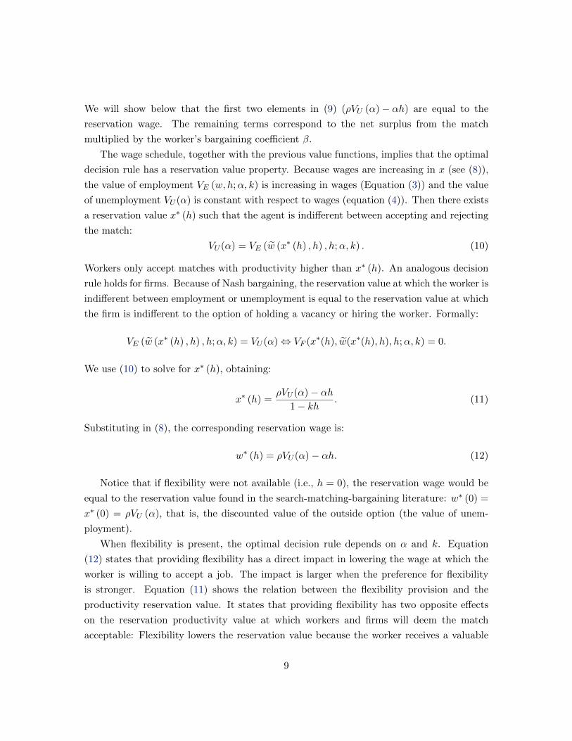
Figure 1 illustrates the value functions for the employment and unemployment states
(equations (3) and (4)), as a function of the match-specific productivity x. Utility max-
imization implies that the optimal behavior is choosing the value function delivering the
highest value for each x. The value of being unemployed, VU (α) , is the horizontal line
that does not depend on wages and is therefore constant with respect to x. The value of
being employed both in flexible and non-flexible jobs is increasing in wages, and therefore,
by Equation (8), it is increasing in x. However, again by (8), workers in a non-flexible job
receive more surplus from additional productivity than workers in a flexible job; therefore,
VE (w (x, 0) , 0;α, k) is steeper than VE (w (x, 1) , 1;α, k). For the same reason, when the
productivity is extremely low, workers in flexible jobs are better off because they receive
the benefit of flexibility. Therefore equation VE (w (x, 1) , 1;α, k) has a higher intercept
than equation VE (w (x, 0) , 0;α, k). This configuration is common to both Case 1 and Case
2 equilibria. The difference between Case 1 and Case 2 is the location of the intersection
points.
Case 1 is described in the left panel of Figure 1. For low values of the match-specific
productivity x, agents prefer to reject the match because the value of unemployment is
higher. The point of indifference for switching state is reached at x = x∗ (1) where both
agents are indifferent to the option of leaving the match or entering a match with a flexible
11

6
-
Vu(α)
x
V
VE(w(x, 0), 0;α, k)
x∗(1)x∗(0) x∗∗
6
-x
V
VE(w(x, 0), 0;α, k)
x∗∗ x∗(0) x∗(1)
Vu(α)
Case 1: α > α∗ Case 2: α < α∗
VE(w(x, 1), 1;α, k)
VE(w(x, 1), 1;α, k)
Figure 1: Different equilibrium outcomes
job and a wage determined by the match schedule (8). Between x∗ (1) and x∗ (0) only jobs
with flexibility are acceptable because the value of a job without flexibility is lower than both
the value of job with flexibility and the value of unemployment. Without the job amenity,
jobs would be rejected in this range of productivity values. If x ≥ x∗ (0), non-flexible jobs
are acceptable, but if x ≤ x∗∗, the surplus a flexible job generates is higher than the surplus
a non-flexible job generates, as shown by equation (13). Only for values of match-specific
productivity higher than x∗∗ the optimal decision rule is to accept a non-flexible job with
a wage determined by (8). Finally, monotonicity of the difference (13) guarantees that this
is the optimal decision rule for the rest of the support of x.
Given the optimal decision rules and conditioning on α, the value of unemployment can
be rewritten as:
ρVU (α) = b(α) + λ
∫ x∗∗
x∗(1)[VE (w (x, 1) , 1;α, k)− VU (α)] dG (x) (15)
+λ
∫x∗∗
[VE (w (x, 0) , 0;α, k)− VU (α)] dG (x)
which, after substituting the optimal wages schedules and value functions, becomes:
ρVU (α) = b(α) +λβ
ρ+ η
∫ αk
ρVU (α)−α1−k
[x− ρVU (α)− α
1− k
]dG (x) (16)
+λβ
ρ+ η
∫αk
[x− ρVU (α)] dG (x)
12

This equation (implicitly) defines the value of unemployment VU (α) as a function of the
primitive parameters of the model. Given that G (x) is an increasing function, this equation
has a unique solution.
Case 2: α < α∗ = kρVU (α∗).
By Proposition 1, in this case x∗∗ < x∗ (0) < x∗ (1). Therefore, the optimal decision
rule in this region of the α−parameter support is:
x < x∗ (0) reject the match
x∗ (0) < x accept the match {w (x, 0) , 0}
In Case 2, the added utility of flexibility relative to the cost of providing it is not enough
to generate acceptable flexible jobs: only non-flexible jobs with high enough match-specific
productivity are acceptable to both agents. This case is illustrated on the right panel of
Figure 1. The indifference to the two employment options, x∗∗, occurs in a region in which
agents do not accept matches. Agents prefer employment to unemployment (or a filled job
to a vacancy) only when the match-specific productivity is higher and the optimal choice is
to accept jobs without flexibility.
Given the optimal decision rules and conditioning on α, the value of unemployment can
be rewritten as:
ρVU (α) = b(α) + λ
∫ρVU (α)
[VE (w (x, 0) , 0;α, k)− VU (α)] dG (x) (17)
which, after substituting the optimal wages schedules and value functions, is equivalent to:
ρVU (α) = b(α) +λβ
ρ+ η
∫ρVU (0)
[x− ρVU (α)] dG (x) (18)
Similarly to (16), this equation implicitly and uniquely defines the value of unemploy-
ment VU (α) as a function of the primitive parameters of the model.
The optimal behavior of Case 1 and Case 2 can be summarized as follows:
Definition 2 Given {λ, η, ρ, β, b(α), k,G (x) , H(α)} an equilibrium is a set of values VU (α)
that solves equation (16) for any α ≤ α∗ and a set of VU (α) that solves equation (18) for
any α > α∗ in the support of H (α) .
This definition states that, given the exogenous parameters of the model, we can solve
for the value functions that uniquely identify the reservation values: the reservation values
13

are the only piece of information we need to fully characterize the optimal behavior. The
equilibrium exists and it is unique because equations (16) and (18) admit a unique solution.
The proof involves showing that both equations define a contraction mapping: it is relatively
straightforward in this case because we are integrating positive quantities on a continuous
probability density function.
This definition is also very convenient from an empirical point of view because - as we
will see in more detail in the identification section - we can directly estimate the reservation
values and, from them, recover information about the value functions and the primitive
parameters.
We now characterize the equilibrium unemployment rate. Given that the arrival rate
of matches follows a Poisson process with parameter λ, it can be shown that in an infinite
horizon model the hazard rate out of unemployment r is constant over time:18,19
r(α) = λ(1−G(x∗(1)) if α > α∗ (19)
r(α) = λ(1−G(x∗(0)) if α ≤ α∗ (20)
It can also be shown that the expected duration in unemployment is equal to the inverse of
the hazard rate:1∫
r(α)dH(α)(21)
a result that we will exploit for identification purposes.
Finally, in steady state the flows of workers into employment status should be equal to
the flow out of it. Hence, defining U as the unemployment rate, it must be the case that
U ·∫r(α)dH(α) = η · (1− U), or, equivalently,
U =η∫
r(α)dH(α) + η(22)
which defines the unemployment rate in equilibrium.
We provide now some economic intuition related to the equilibrium characterization.
Because the cost of providing flexibility is higher for highly productive matches, only rela-
tively lower productivity matches will be associated with flexible jobs. In relatively high-
productivity matches, the higher wage compensates the worker for not having a flexible
job. This is a result of the bargaining process: Because workers share a proportion of the
18See, e.g., Flinn and Heckman (1982). The hazard rate out of unemployment h is defined as the probabilityof leaving unemployment conditional on the worker having been unemployed for a given length of time.
19The hazard rates depend on α because the reservation productivity levels depend on α. See Footnote15.
14

surplus generated by the match, there will always be a value of the rent high enough that
more than compensates the utility gain of working in a flexible job.20 For similar reasons,
if a worker has a significant utility from flexibility and the productivity is low enough, it
will be optimal to give up some of the relatively small share of surplus to gain job flexibil-
ity. The range of productivities over which flexible jobs are accepted is directly related to
preferences because a higher α means that the distance between the two reservation values
x∗∗ and x∗ (1) is larger. Section 4 describes the direct implication of this result on observed
wages, which provides a useful relationship between the data and the model parameters
that is exploited for the empirical identification.
Observe in the left panel of Figure 1 that the interval [x∗ (1) , x∗ (0)] identifies matches
that would have not been created without the flexible job option. This interval illustrates
an efficiency gain of having the option to offer flexible jobs. If the flexibility option were
not available, fewer matches would be created, leaving more jobs unfilled and more workers
unemployed.
4 Identification
The parameters to be identified are the bargaining power β, the parameters of the distribu-
tion over the match-specific productivities G(x), the match arrival rate λ and termination
rate η, the discount rate ρ, the utility flow during unemployment b, the cost of providing
flexibility k, and the distribution over preferences for flexibility H(α). We discuss identifi-
cation based on data containing the following information: accepted wages, unemployment
durations and an indicator of flexibility. We denote it with the set:
∆ ≡ {wi, ti, hi}Ni=1
If the drawback of our approach is the reliance on some functional form assumptions for
identification, one advantage is the relatively minor data requirement needed for the esti-
mation.
The bargaining power parameter. The separate identification of this coefficient is
difficult without demand side information; therefore, we resort to a common assumption in
the literature, which is to assume symmetric bargaining, or β = 1/2.21
20To be precise, this is true if the sampling productivity distribution is not bounded as above. If there isan upper bound to productivity and the share at this upper bound is small enough, it is possible that somehigh α-types will never work in a non-flexible job.
21See Flinn (2006) and Eckstein and Wolpin (1995).
15

The “classic”search-matching model parameters. These are the parameters in-
cluded in the set:
Θ (α) ≡ {λ, η, ρ, b (α) , G(x)}
conditioning on a given type α. Our discussion can then be replicated for each type as long
as the types are identified.
The proof of identification of Θ (α) from the vector of data ∆ was first proposed by
Flinn and Heckman (1982). First, they established that the only features of the model that
can be identified nonparametrically are the reservation wage (identified by the minimum
observed wage) and the hazard rate out of unemployment (identified by the inverse of the
average duration in unemployment). As a result, a distributional assumption on the match
distribution G(x) is necessary to identify the structural parameters in the set Θ (α).
Second, they proved that the distributional assumption must be such that G(x) is re-
coverable.22 This condition arises because they observe only the accepted wage distribution
but they want to identify the offered wage distribution. In our case, we want to identify
the sampling distribution of match-specific productivity, using the accepted wage distribu-
tion. Therefore, our model requires the same parametric assumption because the sampling
distribution maps into wage offers through the optimal Nash bargaining solution. We can
therefore identify the wage offers distribution from the accepted wage distribution, thanks
to the recoverability condition. Then, we can identify the productivity distribution G(x)
by inverting the mapping wage-productivity implied by Nash bargaining.
Third, once the reservation values, the hazard rate out of unemployment and the sam-
pling distribution G(x) are identified, equations (19) and (20) identify λ and equation (22)
plus knowledge of the unemployment rate identify η.
Finally, the parameters ρ and b (α) can only be jointly identified. This is the case
because they contribute to the mapping from the data to the parameters only through the
discounted value of unemployment ρVU (α). This value is not a primitive parameter but
an implicit function of various parameters (see equations (16) and (18)).23 If ρVU (α) is
identified, then ρ and b (α) can be jointly recovered using the equilibrium equation that
implicitly defines ρVU (α).
22A distribution G is recoverable from a truncated distribution with known truncation point z if knowledgeof G(x|x ≥ z) and z implies that G is uniquely determined. Examples of recoverable distributions includethe Normal and the Log-normal.
23Postel-Vinay and Robin (2002) have one of the few articles providing direct estimates of the discountrate within a search framework. Their model is, however, not comparable to ours because the discountrate includes both “impatience” (as in our model) and risk aversion. They generate high estimates forthis parameter: about 12% for the skilled group and up to 65% for some unskilled groups in some specificindustries.
16

Cost to provide and preferences for flexibility. This is set of parameters that
is specific to our model and not commonly found in the literature: the distribution of
preferences for flexibility α and the cost of providing flexibility k.
Heterogeneity in preferences for flexibility helps us fit the data we observe. For example,
if there were only one type of worker with 0 ≤ α < kρVU (0), then in equilibrium we would
observe only non-flexible jobs. If instead there were only one type with kρVU (α) ≤ α, then
we could observe workers in both types of jobs. However, the wage distributions of the
two jobs would have non-overlapping support, something we do not observe in the data.
Multiple types generate an accepted wage distribution as a mixture of distributions (one for
each type) that is capable of better fitting the data we observed for flexible and non-flexible
jobs.
More formally, we follow what is now a standard approach in the literature and assume
a discrete distribution H(α), implying a finite number of values αj , J = 0...T .24 We then
call pj , j = 0...T the proportion of individuals with a preference for flexibility αj (or, more
concisely, the frequency of individuals of type j). The set of parameters left to be identified
is therefore:
Υ ≡ {α,p, T, k}
where α and p are vectors of dimension T + 1.
We proceed by steps, first focusing on the identification of α,p and k given the number
of types and assuming we know how to group individuals by type. Then we expand our
analysis to the case in which we do not observe workers’ types.
When types are observed, identification of p is trivial, and it is given by the proportion
of workers that belong to each type. The identification of the other parameters is more com-
plex, and it depends on the categorization of equilibrium types illustrated in the previous
section. For αj such that αj > kρVU (αj) (equilibrium Case 1), the accepted wage distribu-
tions of flexible and non-flexible jobs do not have a connected support.25 This is because
the marginal worker that does not accept a flexible job, the worker with productivity x∗∗,
receives a compensating differential for the lack of flexibility: w (x∗∗, 1)= w (x∗∗, 0)−α. The
productivity thresholds therefore define bounds in the support of the wage distributions we
24See, e.g., Wolpin (1990), Eckstein and Wolpin (1995) or Eckstein and van den Berg (2007)).25Throughout the identification discussion and in the empirical application, we assume the support of
G (x) is equal to the positive real line. This seems a fairly reasonable assumption because x represents theproductivity of a job match.
17

can use to identify some structural parameters. From equations (8), (11) and (14) we have:
w (x∗ (1) , 1) = ρVU (αj)− αj (23)
w (x∗∗, 1) = β (1− k)αjk
+ (1− β) [ρVU (αj)− αj ] (24)
w (x∗∗, 0) = βαjk
+ (1− β) ρVU (αj) (25)
Solving this system of equations, we obtain:
αj = w (x∗∗, 1;αj)− w (x∗∗, 0) (26)
ρVU (αj) = αj + w (x∗ (1) , 1) (27)
k = βαj
[w (x∗∗, 0)− (1− β) ρVU (αj)
]−1(28)
These three equations state that the size of the discontinuity in the wage support identifies
the preference for flexibility, which is the compensating wage differential for the marginal
worker accepting a non-flexible job. The minimum wage in the sample of observations
belonging to type αj identifies the discounted value of unemployment. The location of
the discontinuity identifies k. The same intuition holds for any αj such αj > kρVU (αj);
therefore, the model is over-identified because there is only one flexibility cost k.
For any αj such αj < kρVU (αj) (equilibrium Case 2 in the previous section), all of
the accepted jobs are non-flexible and flexibility has no impact on the variables that we
can observe. Therefore, we cannot identify αj in this case. We denote all types α′j such
that this is the case with α0 and normalize α0 to zero. This should not have a major
impact in our results and counterfactuals because in the estimation, we obtain values of
αj > kρVU (αj) that are quite low (between 0.1 and 0.01), and α0 must be smaller than the
smallest estimated αj > kρVU (αj).
We now focus on the identification of α,p and k, given T without assuming we know
the workers’ types. In this case, the observed wage distribution is a mixture of wage
distributions over the T + 1 types and we want to identify the proportions in the mixture
(p) together with the values of the (αj’s). Because the discontinuity in the accepted wage
support for one type may overlap with a region without discontinuity for another type, the
mixture may not exhibit the discontinuity we used for identification in the previous case.
However, the mixture will still exhibit a drop in probability mass in correspondence with
the discontinuity in the accepted wage distribution for a given type. This is because in this
region that type does not place any probability mass. As a result, the presence of a drop in
the accepted wage distribution signals the presence of an αj−type such that αj > kρVU (αj).
18

From equation (26), we also know that the width of the support over which the drop occurs
identifies the size of the αj . The height of the drop identifies the proportion pj : the stronger
the drop the higher the proportion of that specific type in the population. The location of
the drops with respect to the lowest accepted wage identifies k because k is proportional
to the distance [w (x∗∗, 0)− w (x∗ (1))], as shown in equation (28). The density of the wage
distribution exhibits drops, and the presence of different types with different α′js smooths
out the kinks. The degree of smoothness depends both on the total number of types present
and on the relative proportion of the types in the population.
Finally, the number of types T , with αj such that αj > kρVU (αj) is identified by the
number of discontinuities in the support of the accepted wage distribution and/or by the
number of drops in the density of the accepted wage distribution.
5 Data
For identification purposes, we need a data set reporting accepted wages, unemployment
durations, a flexibility indicator, and some information regarding age and schooling to select
a relatively homogenous estimation sample.
Finding a good flexibility indicator is a difficult task: ideally, we would like to have a
variable indicating if the worker can freely choose how to allocate her working hours. In
principle, this type of information is observable (e.g., some labor contracts have a flextime
option, allowing workers to enter and exit the job at her chosen time or allowing workers to
bundle extra working hours to gain some days off). However, there is lack of an homogenous
definition across firms and industries of these types of contract. For this reason, we use a
limited but transparent and comparable definition of flexibility that allows us to use a
standard and representative sample of the U.S. labor market. The definition of flexibility
we use is based on hours worked under the assumption that working fewer hours per week is
a way to obtain the type of flexibility we are interested in. For comparability across workers
with different flexibility choices, we measure wages in dollars per hour.
The data is extracted from the Annual Social and Economic Supplement (ASES or
March supplement) of the CPS for the year 2005. We consider only women who declare
themselves as white, who are in the age range 30-55 years old, and who belong to two
educational levels: those who completed high school (high school sample) and those who
completed college at least (college sample). To avoid outliers and top-coding issues, we trim
hourly earnings, excluding the top and the bottom 1% of the raw data.
The variables that we extract are on-going unemployment durations observed for individ-
19

Females College High School
N. flexible 264 240
N. non-flexible 1058 854
Average wage, flexible 22.5 (14.2) 10.3 (4.3)
Average wage, non-flexible 23.4 (10.3) 13.9 (5.9)
Wage range, flexible 2.4-70 2.13-26.7
Wage range, non-flexible 7-57.7 3.65-38.5
Avg. hours worked, flexible 21.3 (7.7) 23.4 (7.6)
Avg. hours worked, non-flexible 42.7 (6.4) 40.5 (3.8)
N. unemployed 34 72
Avg. unemployment duration 4.4 (5.2) 4.6 (5.9)
Table 1: Descriptive statistics (standard deviations in parenthesis)
uals currently unemployed (ti); accepted wages observed for individuals currently employed
(wi) and the flexibility regime (hi) in which the worker is assumed to be in a flexible job
if she is working less than 35 hours per week. We obtain a sample for which descriptive
statistics are presented in Table 1. Accepted earnings are measured in dollars per hour and
unemployment durations in months.
6 Estimation
The minimum observed wage is a strongly consistent estimator of the reservation wage26.
In our model, we can exploit this property of observed minimum wages in both flexible
and non-flexible jobs because it refers to the reservation wage of two different types of
individuals: the lowest accepted wage at non-flexible jobs is a strongly consistent estimator
for the reservation wage of workers’ type such that α < kρVU (α), while the lowest accepted
wage at flexible jobs is a strongly consistent estimator for the reservation wage of workers
who belong to one of the types satisfying α > kρVU (α). Without loss of generality, we
assume this: the lowest accepted wage of a flexible job pertains to type T.
To summarize, the first step of our estimation procedure uses equation (12) to obtain
the following strongly consistent estimators:
ρVU (0) = mini{wi : hi = 0} (29)
ρVU (αT )− αT = mini{wi : hi = 1}
26See Flinn and Heckman (1982)
20

We estimate the remaining parameters in a second step using a Simulated Method of
Moments (SMM) procedure in which, for a given parameters vector, we simulate moments
that we compare with the corresponding moments obtained from the data sample.27
We estimate λ and η by matching two moments exactly: the mean duration of unemploy-
ment spells as equal to the hazard rate (see (21)), which, together with the unemployment
rate (22), defines a system of two linear equations in two unknowns (λ and η).
Assuming G(x) is lognormal with parameters (µ, σ),28 the remaining vector of parame-
ters is defined by θ ≡ {µ, σ, k, α,p,ρVU (α−j)} and is estimated as:
θ = arg minθ
Ψ (θ, t,w,h)′WΨ (θ, t,w,h) (30)
such that Ψ (θ, t,w,h) =[ΓR
(θ|ρVU (0); ρVU (αj)− αj
)− γN (t,w,h)
]where γN is the vector of the sample moments obtained by our sample of dimension N , and
ΓR
(θ|ρVU (0); ρVU (αj)− αj
)is the vector of the corresponding moments obtained from a
simulated sample of size R conditional on the estimated values of ρVU (0) and ρVU (αj)− αj .Bold type represents vectors of variables: for example t is the vector of the unemployment
durations ti. The weighting matrix W is a diagonal matrix with elements equal to the
inverse of the bootstrapped variances of the sample moments.
The moments we match are extracted from the unemployment durations and from the
accepted wages distributions at flexible and non-flexible jobs. For the unemployment du-
rations, we simply compute the mean and the proportion of individuals in unemployment.
For the wage distributions, we exploit that with multiple types of workers, workers with
flexible and non-flexible jobs have accepted wage distributions with overlapping support.
We attain that by computing means and standard deviations of wages at flexible and non-
flexible jobs over various percentile ranges defined by accepted wages at non-flexible jobs.
In addition, we need to use enough moments of the wage distribution in order to capture the
“drops” that correspond to the discontinuous support of the wage distributions of a given
type. We use percentiles 0, 20, 40, 60, 80 and 100 of the non-flexible workers’ accepted wage
distribution to define 5 intervals. Within these 5 intervals, we compute the proportion of
workers holding flexible jobs and the mean and standard deviations of wages with flexible
27In principle, one could attempt a maximum likelihood approach. This is difficult in our model becauseeach type α such that α > kρVU (α) defines a parameter-dependent support over flexible and non-flexiblejobs and the first step allows the estimation of only one such type α. The support of the variables over whichthe likelihood is defined depends on parameters and, therefore, a standard regularity condition is violated.
28This is the most commonly assumed distribution in this literature because it satisfies the recoverabilitycondition for the identification of its parameters and it provides a good fit for observed wages distributions.
21

Parameter College High School
µ 3.5343 (0.0066) 3.0107 (0.0116)
σ 0.5378 (0.0056) 0.4841 (0.0075)
η 0.0057 (0.0016) 0.0136 (0.0026)
λ 0.2288 (0.0504) 0.2196 (0.0355)
α1 0.1035 (0.0609) 0.0100 (0.00004)
p1 0.1256 (0.0103) 0.2084 (0.0337)
α2 0.0100 (0.00003) 0.0255 (0.0120)
p2 0.2437 (0.0119) 0.1641 (0.0202)
k 0.0004 (0.00004) 0.0006 (0.00005)
ρVU (0) 7.0000 (0.0211) 3.6500 (0.2449)
ρVU (α1) 15.3092 (5.1034) 3.9059 (0.8017)
ρVU (α2) 2.4100 (1.1328) 2.1555 (0.1250)
Loss function 46.561 3.671
N 1,356 1,166
Table 2: Estimation results (bootstrapped standard errors from 140 samples in parenthesis)
and non-flexible jobs.29
7 Results
The model is estimated separately from data regarding women with a high school degree and
regarding women with at least a college degree. The implicit assumption is that the labor
market is segmented along observable workers’ characteristics so that the two education
groups do not compete for the same jobs. This assumption is consistent with the ex-ante
homogeneity condition imposed in the theoretical model and with previous literature on the
estimation of search models.30
The specification of the unobserved heterogeneity in preferences for flexibility includes
three types. Due to the non-identification result discussed in Section 4, for the Case-2
equilibria with αj < kρVU (αj) (such that workers only accept non-flexible jobs) we set
α0 = 0. We estimated the model with four types, but the specification did not generate a
significant improvement of the model fit.31
Estimated parameters are reported in Table 2. The parameter estimates fit the data
well (see the table in the the Appendix A.3) and therefore provide a reasonable base for the
29The complete list of the simulated moments is in the Appendix A.3.30See, for example, Bowlus (1997) and Eckstein and Wolpin (1995).31The value of α estimated for the additional type converged to the value of α of one of the existing types,
and the proportion of workers associated to the additional type in the population was negligible.
22

counterfactuals we conduct in the next section. Observe first that arrival rates, termination
rates, and the two parameters of the lognormal distribution of match-specific productivity
are comparable to the corresponding values obtained in the literature.32 The arrival rates
imply that agents receive an offer, which they may accept or reject, about every 4 months on
average. The sampling productivity distribution parameters (µ, σ) imply that the average
productivity of college graduates is almost $40 per hour while the average productivity of
high school graduates is about $23 per hour. The reservation wages should be interpreted
as measured in dollars per hour, and they appear to be within a reasonable range.
The flexibility-related parameters have plausible values: about 37% of college educated
women are willing to pay between 1 and 10 cents per hour to work in flexible jobs. Firms’
cost of providing flexibility is 0.04% of the hourly potential productivity. A similar propor-
tion of women with a high school education value flexibility, but they are willing to pay a
lower dollar amount (between 1 and 2.5 cents per hour), while firms face a higher cost of
providing it, about 0.06% of the hourly potential productivity.
We have a very limited model of the firms side of the market, so it is difficult to find
an explanation about why firms employing low-skilled workers may have higher cost of
flexibility. Although firms needing only workers with lower skills makes it easier to substitute
workers, secretarial and manual jobs are often performed in teams and may require a higher
need for coordinating work-hours among workers than professional jobs.
The difference between the parameter estimates on high-school and college graduates
suggests that women might choose schooling in part to accommodate a preference for job
flexibility. Schooling is costly, but it provides access to jobs with relative low cost of flex-
ibility. This might provide a partial explanation to the puzzle of why women have lower
wages than men but acquire more schooling.33
8 Counterfactual Policy Experiments
We present two counterfactual experiments to assess the importance of flexibility. To com-
pute the equilibrium and derive welfare implications under each experiment’s assumptions
we need, in addition to the estimates presented in the previous section, estimates of the flow
32See, for example, Flabbi (2010) and Bowlus (1997), who estimated comparable search models on samplesof women. Flabbi used CPS 1995 data on white college graduates finding a very similar arrival rate andslightly lower average productivity in the presence of employers’ discrimination. Bowlus used a NationalLongitudinal Survey of the Youth 1979 sample of college and high school women, finding a slightly lowerhazard rate of unemployment in the presence of a non-participation state.
33The main explanations proposed so far have focused on the positive returns in the marriage market, seeChiappori, Iyigun and Weiss (2006) and Ge (2008).
23

values of unemployment b(αj). Because ρ and b (αj) are only jointly identified, we adopt a
common assumption in the literature and fix the discount rate ρ = 0.05 and recover b(αj)
using the equilibrium equations (16) (for j = 1, 2) and (18) (for j = 0).34
To summarize, we base the experiments on the following set of structural parameters:{µ, σ, η, λ, α, p, k, b(α)
}We compute the equilibrium under the assumptions of each experiment, and we use it to
generate simulated samples of 100,000 labor market careers. From the samples we compute
various labor market statistics which we compare to a sample derived from the parameter
estimates (which we refer to as the benchmark model). Table 3 presents these statistics
for the benchmark model. Tables 4 and 5 compare the same statistics, obtained under the
assumptions of each experiment, with those from benchmark model. The first row in each of
these tables shows the discounted value of unemployment ρVU (α), which can be interpreted
as a measure of welfare because VU (α) is the present discounted value of participating in
the labor market for a potential worker of type α. The next set of rows report statistics
about workers in non-flexible and (when present) flexible jobs: the average and standard
deviation of accepted wages and the percentage of employed individuals of a given type
working in each flexibility regime. The next two rows present the average unemployment
duration and the unemployment rate. The last set of rows display firms’ per-worker and
total profits from flexible and non-flexible jobs.35
8.1 Counterfactual 1: No flexibility
To understand the impact of flexibility, we ask how much the labor market outcomes of
women would change if flexibility were not available. To answer this question, the first
policy experiments imposes that all jobs must be non-flexible. All parameters are set at
their estimated values.
In this new environment, the only decision workers have to make is between accepting
or rejecting a wage offer at a non-flexible job. Therefore, the optimal decision rule is
characterized by only one reservation value for each type of worker, which we obtain by
equating the value of unemployment and the value of employment at a given wage. This
34Flinn and Heckman (1982) use a value of 5% and 10%, and Flinn (2006) uses 5%. We performedsensitivity analysis and found that doubling discount rate to 10% does not make an appreciable differenceon the results.
35The values in the ”All” column are not simple averages of each group’s mean but averages computed onthe overall relevant sample.
24

College High School
α0 α1 α2 All α0 α1 α2 All
ρVU (α) 7.000 15.309 2.410 6.925 3.650 3.906 2.156 3.458
Workers in non-flexible jobs
Mean wage 23.335 172.338 25.433 23.803 13.242 16.008 27.685 13.932
St. dev. wages 11.367 29.763 10.998 11.462 5.833 5.499 6.273 6.097
% of workers 100.00 0.007 69.971 80.125 100.00 66.236 6.432 77.608
Workers in flexible jobs
Mean wage . 28.392 10.730 21.880 . 8.118 11.448 10.401
St. dev. wages . 11.246 2.279 12.424 . 1.412 4.190 3.880
% of workers 0 99.993 30.029 19.875 0 33.764 93.568 22.392
Unemployed workers
Avg. unempl. dur. 4.378 4.677 4.371 4.414 4.556 4.556 4.555 4.556
Unempl. rate 0.024 0.026 0.024 0.024 0.058 0.058 0.058 0.058
Firms’ profits
Average (non-flexible) 16.335 157.028 23.023 17.778 9.592 12.102 25.530 10.257
Average (flexible) . 13.187 8.330 11.395 . 4.222 9.318 7.716
Table 3: Benchmark model, computed using the parameter estimates. “.” refers to missingobservations.
equilibrium equation - the equivalent of equation (11) in the pre-policy environment - is:
x∗ (0) = ρVU (αj) (31)
The new equilibrium is then defined by a set of VU (αj) that solve the equation:
ρVU (αj) = b (αj) +λβ
ρ+ η
∫ρVU (αj)
[x− ρVU (αj)] dG (x|µ, σ) (32)
which corresponds to equation (18) in the benchmark model.
This experiment has two unambiguous implications in terms of labor market outcomes.
First, agents with preferences for flexibility have a lower value of participating in the labor
market because a job amenity that they value is not available. We can measure this impact
by comparing the present discounted value of unemployment VU (αj) with or without the
policy. Second, the range of productivities that correspond to acceptable job matches is
smaller than in the benchmark model. This can be understood by looking at the left panel
in Figure 1. The range between x∗ (1) and x∗ (0) defines productivities where only flexible
25

College High School
α0 α1 α2 All α0 α1 α2 All
ρVU (α) = 99.58 99.92 99.88 = 99.96 99.33 99.92
Workers in non-flexible jobs
Mean wage = 16.43 82.39 98.22 = 83.79 44.99 94.38
St. dev. wages = 38.05 104.54 101.10 = 107.16 93.07 96.03
% of workers = 1412473.1 142.91 124.80 = 150.97 1554.80 128.85
Unemployed workers
Avg. unempl. dur. = 100.06 100.00001 100.01 = 100.0004 100.00001 100.0001
Unempl. rate = 100.05 100.00001 100.01 = 100.0004 100.00001 100.0001
Firms’ profits
Per worker = 8.32 80.55 92.60 = 78.58 40.40 94.50
Total = 9258.14 115.10 115.54 = 118.60 622.49 121.76
Table 4: Counterfactual 1, No flexibility. Benchmark model = 100, “=” refers to no change
jobs are accepted. If we remove this job option, a portion of jobs in this range will remain
unfilled.
Both of these impacts are very modest: Table 4 shows the decrease in VU (αj) is present
for all the types that value flexibility, but the amount of the decrease is between 0.04 and
0.42 percent. The impact on the unemployment rate and unemployment duration is even
smaller: they both increase after the policy for all the types that value flexibility, but the
increase is between 0.06 percent and less than a thousandth of a percentage point.
The impacts are small for two reasons. First, the estimates of the utility value attached
to flexibility is relatively modest and therefore dropping this amenity is not a big cost. The
second reason is less trivial. In our model, workers accepting flexible jobs optimally react
to the new environment by taking non-flexible jobs instead of becoming unemployed, which
allows them to offset the impact on total welfare.
The implications for the distribution of accepted wages are ambiguous. First, accepted
wages of agents with positive α change in two opposite directions. There is a positive
effect because all of the jobs are non-flexible. There is no wage cut due to the provision of
flexibility. There is a negative effect because the workers’ outside option in bargaining with
the firms, VU (αj), is lower. The outside option is lower because the labor market does not
provide an amenity that the workers value. Second, the composition of the productivity
distribution of the accepted non-flexible jobs is different: The accepted non-flexible jobs
are on average less productive than the accepted non-flexible jobs in the pre-policy regime
because in the pre-policy regime, low productivity matches were associated with flexible
26

jobs.
The results show that the negative effects dominate. The average wages for types that
value flexibility is considerably smaller, ranging from 16.4% of the average wage in the
benchmark model for the α1−type in the college sample to 83.8% for the α1−type in the
high school sample.
The impact on the proportion of employed individual working in flexible and non-flexible
jobs is huge for types working mostly flexible jobs in the pre-policy regime. Only 0.007%
of the α1−type in the college sample is working in flexible jobs in the pre-policy regime,
while now 100% of them is forced to work in non-flexible jobs. Accordingly, the proportion
of workers working in non-flexible jobs increases by about fourteen thousand times. The
impact on profits on types with a high value of flexibility is large due to composition effects.
For example, the average profit firms make on the α1−type in the college sample is a small
fraction of the pre-policy profit, but this is because more α1−types work in flexible jobs
after the policy change, generating a large increase in total profits.
To summarize, the impact of the presence of flexibility is large on some labor market
outcomes (i.e., wages and hazard rates, redistribution of employment from flexible to non-
flexible jobs) but negligible on others (unemployment).
8.2 Counterfactual 2: Reduction of the cost of flexibility
The second experiment considers policies that ease the provision of flexible jobs by reducing
their cost. We implement a reduction of k to one half of its estimated value. A lump-sum
tax on all workers finances the cost reduction. A similar policy implemented at zero cost
to both workers and employers leads to very similar results, and it is not reported.36
The model is characterized by the same structural parameters of the benchmark model
plus the tax rate. The tax rate is endogenous, and it is defined as the tax rate necessary
to support in equilibrium a cost reduction of k to one half of its estimated value. The
new equilibrium is analogous to the one obtained in the Section 3, with the addition of
the derivation of the tax rate. Details of such derivation are in the Appendix A.4. To
quickly illustrate the difference with respect to the benchmark case, we only report here
the reservation match value in this new environment:
x∗ (h|αj) =ρVU (αj) + t− αjh
1− kh(33)
Because workers have to pay a tax when accepting a job, the direct impact of the tax
36Results of the no-tax policy experiment are reported in Flabbi and Moro (2010).
27

rate on the productivity value at which a job becomes acceptable is positive. The overall
impact depends on the direct impact and on the equilibrium impact of the tax rate on the
value of unemployment VU (αj).
Because it is a is lump-sum tax, and it does not depend on the preferences for flexibility,
the policy also impacts workers who do not value flexibility. We expect an increase in
welfare for workers that value flexibility and a decrease for those who do not. The increase
in welfare is due to the provision of flexibility at a lower cost: Because workers who value
flexibility share this cost with the employers (due to bargaining) and with the workers who
do not value flexibility (by the design of the lump-sum tax), any cost reduction is beneficial
to them.
The results, reported in Table 5, show that the welfare effects are very small. The
increase in welfare (first row of the table) for the α1− and α2−types is only between 0.01 and
0.13 percentage points. The decrease in welfare for the α0−type is less than a thousandth
of a percentage point. The result is due to the fact that the flexibility cost is very low in
the benchmark model. Therefore, the cost reduction implied by the experiment is relatively
modest.
An effect of the policy is the potential for efficiency gains. Because flexibility is cheaper,
there is the potential for an increase of the range of productivities associated with acceptable
jobs. To study whether this is the case, we have to look at the lower and upper bounds
of this range. The impact on the upper bound is unambiguous. The upper bound is the
reservation productivity value at which workers decide to work non-flexible jobs instead of
flexible jobs. It is defined by equation (14) as the ratio between the preference for flexibility
and the cost of its provision. Because the policy implies a lower cost of flexibility, the upper
bound will be higher, contributing to a larger range. The impact on the lower bound is,
instead, ambiguous. The lower bound is equal to the reservation productivity value at which
jobs start to become acceptable, and it is defined in equation (33). After the policy, the
numerator increases due to the increase in ρVU (α) and to the presence of the tax rate. The
denominator increases due to the decrease in k. The overall impact is therefore ambiguous.
However, we know from the first row of Table 5 that the increase in ρVU (α) is very small.
Therefore, we expect the second effect to dominate, leading to a decrease in x∗ (h|α). A
lower reservation values means that some productivity ranges that were not acceptable
before are now acceptable, leading to a decrease in unemployment. In the simulation, this
decrease turns out to be negligible, with an order of magnitude of one thousandth of a
percentage point on the type with the highest utility from flexibility.37
37On the other types valuing flexibility the change is so small as to approximate 100 up to the fifth decimal.
28

College High School
α0 α1 α2 All α0 α1 α2 All
ρVU (α) 99.9999 100.01 100.13 100.01 99.9999 100.08 100.06 100.03
Workers in non-flexible jobs
Mean wage 99.72 179.00 148.01 102.72 100.02 148.56 181.01 98.93
St. dev. wages 100.91 118.70 99.37 109.62 100.83 102.69 143.28 104.25
% of workers = 0.24 31.73 85.47 = 23.47 2.46 85.06
Workers in flexible jobs
Mean wage . 99.68 150.95 96.05 . 140.53 108.09 114.17
St. dev. wages . 99.31 237.94 81.47 . 234.98 134.74 118.95
% of workers 0 100.01 259.07 158.57 0 250.14 106.70 151.77
Unemployed workers
Avg. unempl. dur. 100.0001 99.9985 100.00 99.9998 100.0002 100.0001 100.00 100.0004
Unempl. rate 100.0001 99.9986 100.00 99.9998 100.0001 100.0001 100.00 100.0003
Firms’ profits
Avg. (non-flexible) 99.60 186.70 153.02 100.19 100.03 164.20 187.84 98.67
Total (non-flexible) 99.60 169.73 48.63 85.64 100.03 38.62 6.36 83.94
Avg. (flexible) . 99.29 165.58 118.59 . 177.86 109.93 114.41
Total (flexible) . 99.30 428.62 188.06 . 444.51 117.30 173.58
Table 5: Counterfactual 2: half flexibility cost financed by lump-sum tax. Benchmark model= 100), “=” refers to no change, “.” refers to missing observations.
Because flexibility is cheaper and preferences are unchanged, we expect a transfer of
employed workers from non-flexible jobs to flexible jobs. We also expect a greater in-flow
to employment in flexible jobs from unemployment because the reservation productivity
value at which workers will accept a flexible job is lower. As a result, the proportion of
the employed working in flexible jobs increases. This is the first margin where we observe
large effects. The seventh row of Table 5 shows that the increase is large (about 2 and
half times) for the α2-type in the college sample and the α1-type in the high-school sample.
These are types that value flexibility but still had more than half of the workers employed
in non-flexible jobs in the benchmark model. The increase is smaller on the other two types
valuing flexibility because almost all the workers were already employed in flexible jobs in
the benchmark model.
The equilibrium impact on average wages is complex and takes place through five differ-
ent channels. The first three channels lead to an increase in average wages in both flexible
and non-flexible jobs. First, the lower cost of flexibility has a positive impact on wages be-
29

cause the savings generated by the lower cost are split between workers and firms. Second,
the equilibrium effect on the reservation wage is positive because the reservation wage is
directly proportional to ρVU (α), which is increasing. Third, the composition in terms of
productivity of workers working in flexible and non-flexible jobs is changing. The transition
from non-flexible jobs to flexible jobs involves productivity ranges that are low with respect
to non-flexible jobs in the benchmark model but high with respect to flexible jobs in the
benchmark model. Therefore, the average wage will increase in flexible jobs because of the
in-flow of high productivity workers and will also increase in non-flexible jobs because only
the most productive workers will remain there. The fourth channel works through the lower
reservation productivity value at which workers accept a flexible job. Because the reserva-
tion productivity value is lower, there is an in-flow of relatively low productivity workers
into flexible jobs, leading to a negative impact on the average wage of workers in flexible
jobs. The fifth and last channel is the presence of the tax. However, the tax generates
a negligible impact in labor market outcomes because the cost of flexibility is very low.
Therefore, the tax required to finance it is extremely low.
The results show that the first three channels dominate on all types with the exception
of type α1 in the college sample. Average wages increase by about 50 percent or more
in non-flexible jobs for both α1 and α2 types on both the college and high-school sample.
Wages also increase in flexible jobs: by about 50 percent on type α2 in the college sample
and by about 40 percent on type α1 in the high-school sample. For the college sample type
α1, they decrease slightly (see the fifth row and second column of Table 5). Almost all
workers of this type were employed in flexible jobs in the pre-policy regime; therefore, they
are the most sensible to the wage compression due to the lower reservation productivity
value (the fourth channel described above).
There are also economically significant impacts on profits. Starting with α2−type,
workers with a college education, we observe that the average profits in non-flexible jobs
increase. The increase is due to the redistribution of workers from non-flexible jobs to
flexible jobs: with respect to the pre-policy environment, fewer but more productive matches
are realized without flexibility. Therefore, overall profits will decrease, and average profit
will increase. Over this type of workers, the average profits at flexible jobs also increase.
This is because the additional surplus generated by the lower cost of flexibility is not fully
appropriated by the worker, but it is partially distributed to the firm. The only type over
which profits do not increase is type α1 in the college sample. Similarly to what happens
on wages, the reservation productivity value at which jobs become acceptable decreases,
leading to lower average and total profits.
30

One general conclusion from the policy experiments is that the impacts are generally
small, due to the relatively low utility value associated with flexibility. However, despite the
small magnitude of the change in policies we are proposing, there is a large effect on wages.
If the policy objective is to impact the wage structure, then policies aimed at reducing the
cost of providing flexibility could be particularly effective. Moreover, if men had significantly
lower preferences for flexibility - as some anecdotal evidence seems to indicate - then these
policies would have the potential to reduce the wage gap because they would increase female
wages proportionally more than male wages.
9 Conclusion
In this paper, we estimate the parameters of a dynamic search model of the labor market
in which workers and firms bargain over wages and the provision of flexibility. We maintain
the narrow definition of flexibility most frequently found in the literature - flexibility as the
availability of part-time work - and show that women value this amenity.
In our estimates, we also find that college graduates and high-school graduates value
flexibility differently. College graduates place higher value on having flexible jobs. Moreover,
we find that jobs requiring a college education can provide flexibility at a lower cost. Because
women might also choose schooling to accommodate their preference for job flexibility, we
speculate that this might explain some of the observed differences in schooling achievements
between men and women.
The counterfactual experiments reveal that the impact of flexibility is quite substantial
on some labor market outcomes (i.e., wages and hazard rates, the distribution of employment
between flexible and non-flexible jobs) but negligible on others (notably, unemployment).
For example, without flexibility, for college-educated women that value flexibility the most,
the average wage would be 74% lower, while the unemployment rate would be at most 0.06%
higher than in the benchmark environment with flexibility. We infer from our experiments
that policies reducing the cost of flexibility provision could be very effective in changing the
realized wage distribution at little cost in terms of employment.
Our approach presents four main limitations. First, in the empirical application of our
model, we define flexible jobs using part-time jobs. A more appropriate definition should
also capture the option of organizing work time in a flexible way.
Second, we estimate the model by schooling groups and we find significant differences
between them. We did not, however, integrate a schooling decision in the model and in
the estimation procedure. We think devoting future work to filling this gap is particularly
31

promising to test our conjecture that expectations on future job amenities, such as flexibility,
are important components of the schooling choices of women.
Third, employers and workers in our model are very stylized. In particular, we assume
a homogenous cost of providing flexibility, and workers are heterogeneous only in education
and preference for flexibility. Estimating heterogeneous costs and correlations between costs
and industries could help explain why we observe different preferences across different skill
levels and could deepen our understanding of the feedback of the labor market on schooling
choices. Just as we find that different levels of schooling are correlated with preferences for
flexibility, we could find that different types of jobs or schooling (e.g., college majors) are
correlated with preferences for flexibility because they increase the likelihood of working in
jobs and industries that provide flexibility at low cost.
Fourth, we have found a strong impact of flexibility on wages and a significant correla-
tion between preference for flexibility and level of schooling. A large amount of literature
on gender differentials on both variables currently points to a puzzle: Recent data on U.S.
workers show women earning lower wages than men, despite having a positive schooling
differential. Results from the counterfactuals reveal that changes in the provision of flexi-
bility (e.g., through a subsidization of its cost) have a large differential impact for people
that value flexibility differently. Therefore, a higher preference for flexibility for women
with respect to men (if proved) could potentially explain a large portion of the gender-wage
differential. Exploring this conjecture requires estimating the model for a sample of men.
Our sample does not include enough males working in flexible jobs to provide reliable esti-
mates of their preferences for flexibility. We hope that a more complete data set providing a
better definition of flexibility (and possibly more detailed schooling and firms information)
will also generate enough data variation to estimate the model on a sample of men.
References
[1] Altonji, J., and C. Paxson (1988) ”Labor Supply Preferences, Hours Constraints, and
Hours-Wage Trade-offs”, Journal of Labor Economics, 6(2): 254-276.
[2] Becker, G. (1967) Human Capital and the Personal Distribution of Income, Ann Arbor,
MI: University of Michigan Press.
[3] Blank, R. (1990) “Are Part-Time Jobs Bad Jobs?”, in G. Burtless (ed.) A Future of
Lousy Jobs? The Changing Structure of U.S. Wages. Washington, D.C.: Brooking
Institution.
32

[4] Blau, D. (1991) Search for Nonwage Job Characteristics: A Test for Reservation Wage
Hypothesis”, Journal of Labor Economics, 9(2): 186-205.
[5] Bloemen, H. (2008), “Job Search, Hours Restrictions, and Desired Hours of Work”,
Journal of Labor Economics, 26(1): 137-179.
[6] Bowlus, A. (1997), “A Search Interpretation of Male-Female Wage Differentials”, Jour-
nal of Labor Economics, 15(4), pg. 625-657.
[7] Burdett, K., and D. Mortensen (1998), “Wage Differentials, Employer Size, and Un-
employment”, International Economic Review, 39(2), 257-273.
[8] Chiappori, P-A., M. Iyigun, and Y. Weiss (2006), “Investment in Schooling and the
Marriage Market”, IZA Discussion Paper 2454
[9] Dey, M., and C. Flinn (2005), “An Equilibrium Model of Health Insurance Provision
and Wage Determination”, Econometrica, 73: 571-627.
[10] Eckstein, Z., and G. van den Berg (2007), “Empirical labor search: A survey”, Journal
of Econometrics, 136: 531-564.
[11] Eckstein, Z., and K. Wolpin (1995), “Duration to First Job and the Return to School-
ing: Estimates from a Search-Matching Model”, The Review of Economic Studies,
62(2): 263-286.
[12] Eckstein, Z., and K. Wolpin (1999), “Estimating the Effect of Racial Discrimination
on First Job Wage Offers”, The Review of Economics and Statistics, 81(3): 384-392.
[13] Flabbi, L. (2010), “Gender Discrimination Estimation in a Search Model with Matching
and Bargaining”, International Economic Review, 51(3): 745-783.
[14] Flabbi, L., and A. Moro (2010), “The Effect of Job Flexibility on Female Labor Market
Outcomes: Estimates from a Search and Bargaining Model”, IZA Discussion Paper
4829.
[15] Flinn, C. (2006), “Minimum Wage Effects on Labor Market Outcomes under Search,
Bargaining and Endogenous Contact Rates”, Econometrica, 73: 1013-1062.
[16] Flinn, C., and J. Heckman (1982), “New Methods in Analyzing Structural Models of
Labor Market Dynamics”, Journal of Econometrics, 18: 115-168.
33

[17] Ge, S. (2008), “Women’s College Decisions: How Much Does Marriage Matter?”,
mimeo, Virginia Tech.
[18] Golden, L. (2001), ”Flexible Work Schedules: What Are We Trading Off to Get
Them?”, Monthly Labor Review, March.
[19] Gronberg, T., and R. Reed (1988), ”Estimating Workers’ Marginal Willingness to Pay
for Job Attributes using Duration Data”, Journal of Human Resources, 29: 911-931.
[20] Hwang, H., D. Mortensen, and R. Reed (1998), ”Hedonic Wages and Labor Market
Search”, Journal of Labor Economics, 16(4): 815-847.
[21] Lang K. and S. Majumdar (2004), ”The Pricing of Job Characteristics When Markets
Do Not Clear: Theory and Policy Implications”, International Economic Review, 45(4):
1111-1128.
[22] Moffitt, R. (1984) “The Estimation of a Joint Wage-Hours Labor Supply Model”,
Journal of Labor Economics, 2(4): 550-566.
[23] Postel-Vinay, F. and J-M Robin (2002), “Equilibrium Wage Dispersion with Worker
and Employer Heterogeneity”, Econometrica, 70(6), 2295-2350.
[24] Rosen, S. (1974), ”Hedonic Prices and Implicit Markets: Product Differentiation in
Pure Competition”, Journal of Political Economy, 82: 34-55.
[25] Rosen, S. (1986), ”The Theory of Equalizing Differences” in: Handbook of Labor Eco-
nomics, V. 1 (O. Ashenfelter and R. Layard, eds.), Amsterdam: North-Holland.
[26] Scandura, T., and M. Lankau (1997), ”Relationship of gender, family responsability
and flexible work hours to organizational commitment and job satisfaction”, Journal
of Organizational Behavior, 18: 377-391.
[27] Topel, R. (1986), ”Local Labor Markets”, Journal of Political Economy, 94: S111-S143.
[28] Usui, E. (2006), ”Gender Occupational Segregation in an Equilibrium Search Model”,
mimeo, Wayne State University.
[29] Wolpin, K. (1990), Estimating a Structural Search Model: The Transition from School
to Work”. Econometrica 55 (July 1987), 801-17
34

A Appendix
A.1 Derivation of Value Functions
The value of employment at wage w and flexibility h for an agent with preference α working
at a firm with flexibility cost k is given by the following discrete time approximation:
VE (w, h;α, k) = (w + αh) ∆t+ (34)
+ ρ(∆t)[(1− η∆t)VE (w, h;α, k) + η∆tVU (α) + o(∆t)]
where ∆t denotes a time span. This expression states that the value of employment is given
by the utility received in the entire period plus the discounted expected value of remaining
at the job or of falling in the unemployment state. Other possible events are happening
with a negligible probability o(∆t). Assuming ρ(∆t) = (1 + ρ∆t)−1 , rearranging terms and
dividing both sides by ∆t, we obtain:
(1 + ρ∆t)
∆tVE (w, h;α, k) = (w + αh) ∆t
(1 + ρ∆t)
∆t+ (35)
+(1− η∆t)
∆tVE (w, h;α, k) +
η∆t
∆tVU (α) +
o(∆t)
∆t
Since the Poisson process assumption implies that lim∆t→0o(∆t)
∆t = 0, when ∆t −→ 0 the
previous expression converges to:
ρVE (w, h;α, k) = w + αh− ηVE (w, h;α, k) + ηVU (α) (36)
After collecting terms, this equation is equivalent to (3).
The value of unemployment for an agent with preference α is given by the following
discrete time approximation:
VU (α) = b(α)∆t+ (37)
+ ρ(∆t)
{(1− λ∆t)VU (α) + λ∆t
∫max [VE (w, h;α, k) , VU (α)] dG (x) + o(∆t)
}This expression states that the value of unemployment is given by the total (dis)utility from
unemployment over the period, equal to b (α) ∆t, and by the fact that after a period ∆t,
two main events may happen: not meeting any firm and remaining unemployed or meeting
a firm, extracting a match-specific productivity value x and deciding whether to accept the
35

job offer or not. We can proceed as with the derivation of VE , obtaining:
(1 + ρ∆t)
∆tVU (α) = b(α)∆t
(1 + ρ∆t)
∆t+
(1− λ∆t)
∆tVU (α) + (38)
+λ∆t
∆t
∫max [VE (w, h;α, k) , VU (α)] dG (x) +
o(∆t)
∆t
Computing the limit to continuous time, this expression becomes:
ρVU (α) = b(α)− λVU (α) + λ
∫max [VE (w, h;α, k) , VU (α)] dG (x) (39)
leading to equation (4) when we collect terms.
Finally, the value of a filled job for a firm with technology k paying a wage w, offering
flexibility h to an agent with preference α is:
VF (pr, h;α, k) = [(1− kh)x− w] ∆t+ (40)
+ ρ(∆t)[(1− η∆t)0 + η∆tVF (pr, h;α, k) + o(∆t)]
Notice that the dependence on the worker’s preference is through the wage schedule,which
depends on α after the bargaining game is solved. Applying the assumption on the discount
function ρ(∆t) and rearranging we get:
(1 + ρ∆t)
∆tVF (pr, h;α, k) = [(1− kh)x− w]
(1 + ρ∆t)
∆t+η∆t
∆tVF (pr, h;α, k) +
o(∆t)
∆t(41)
and taking limits to continuous time:
ρVF (pr, h;α, k) = [(1− kh)x− w] + ηVF (pr, h;α, k) (42)
leading to equation (5) when we collect terms.
A.2 Proof of Proposition 1
Proof. By definition of the reservation values:
x∗∗ ≤ x∗ (0)⇐⇒ α
k≤ ρVU (α)⇐⇒ α ≤ kρVU (α)
Also, by definition of the reservation values, we obtain:
x∗ (0) ≤ x∗ (1)⇐⇒ ρVU (α) ≤ ρVU (α)− α1− k
⇐⇒ α ≤ kρVU (α)
36

proving the claim.
A.3 Matched Moments
We match mean unemployment duration and the proportion of individuals in unemployment
exactly to compute the hazard rate and ρ. To estimate the other parameters, we match
various moments of portions of five interquantiles of the flexible and non-flexible workers’
wage distributions delimited by percentiles 0, 20, 40, 60, 80, and 100 of the non-flexible
workers’ wage distribution. The moments we match are the mean and standard deviation
of wages of workers in non-flexible jobs, the fraction of workers in flexible jobs, and the mean
and standard deviation of wages of workers in flexible jobs. The following table illustrates
the moments in the data and simulated moments at the estimated parameter values.
Non-flexible jobs Flexible jobs
Sample Mean wages St. dev. wages Prop. workers Mean wages∗ St. dev. wages∗
Estim. Data Estim. Data Estim Data Estim. Data Estim. Data
All College 23.715 23.410 11.302 10.360 0.191 0.200 21.836 22.490 12.784 14.152
Quintile 1 12.297 12.032 1.976 2.273 0.311 0.311 3.495 3.447 2.491 2.470
Quintile 2 16.858 17.085 1.124 1.106 0.118 0.122 2.020 2.131 1.798 1.911
Quintile 3 21.141 21.134 1.270 1.352 0.128 0.071 2.701 1.528 2.374 1.469
Quintile 4 26.587 26.574 1.857 2.080 0.163 0.190 4.368 5.037 3.683 4.144
Quintile 5 39.222 39.910 7.783 8.196 0.197 0.195 7.819 8.021 6.483 6.714
All High Sc. 13.933 13.879 6.097 5.923 0.218 0.219 10.512 10.294 3.918 4.279
Quintile 1 7.321 7.532 1.179 1.253 0.379 0.369 2.744 2.765 1.768 1.798
Quintile 2 10.301 10.091 0.718 0.731 0.276 0.277 2.757 2.769 2.008 2.026
Quintile 3 12.718 12.735 0.736 0.770 0.145 0.144 1.846 1.843 1.590 1.609
Quintile 4 15.640 15.559 1.004 1.139 0.146 0.144 2.273 2.223 1.956 1.945
Quintile 5 22.452 22.392 3.974 4.137 0.089 0.084 1.760 1.780 1.622 1.703
∗Because some quintiles may not display any worker in flexible jobs for some parameter
values and because identification relies on the fractions of flexible and non-flexible job
workers with overlapping wage support, means and standard deviations of wages in flexible
jobs were multiplied by the corresponding fraction of workers in flexible jobs (except for the
row displaying moments for all workers).
37

A.4 Derivation of Lump-sum Tax in Counterfactual Experiment 2
The equilibrium characterization of this model is analogous to that obtained in Section 3,
but we also need to compute the tax rate t. Wages and profits result from bargaining over
the surplus. The surplus - represented in the pre-policy environment by equation (6) - now
becomes:
S (x,w, h;α, k) =1
ρ+ η[w − t+ αh− ρVU (α)]β
[(1− k′h
)x− w
](1−β)(43)
leading to the following wage schedule:
w (x, h) = β(1− k′h
)x+ (1− β) [ρVU (α) + t− αh] (44)
This is the wage schedule that corresponds to equation (7) in the pre-policy environment.
As in the benchmark case, the model can be written recursively. The value of unemployment
equations used to compute the reservation values are, for α0 :
ρVU (α0) = b (α0) +λβ
ρ+ η
∫ρVU (α0)+t
[x− ρVU (α0)− t] dG (x|µ, σ) (45)
and for α1, α2 :
ρVU (αj) = b (αj) +λβ
ρ+ η
∫ αjk′
ρVU(αj)+t−αj1−k′
[x− ρVU (αj) + t− αj
1− k′
]dG (x|µ, σ) (46)
+λβ
ρ+ η
∫αjk′
[x− ρVU (αj) + t] dG (x|µ, σ)
where we have already imposed the optimal wage schedule and the optimal decision rule
based on the reservation values:
x∗ (h|αj) =ρVU (αj) + t− αjh
1− k′h
Given these equations the equilibrium is defined as in the benchmark model. To compute
the endogenous tax rate we need to know in equilibrium the proportion of workers who are
employed and unemployed. To obtain these values, it is useful to define the hazard rate
from unemployment to employment in flexible and non-flexible jobs. Given the stationarity
of the model and the Poisson process assumption, the hazard rates are constant and equal
to the probability of receiving an offer multiplied by the probability to accept it. For types
38

α1 and α2, the hazard rate from unemployment to employment in flexible jobs is:
r (h = 1|αj) = λ
[G(αjk′|µ, σ
)−G
(ρVU (αj) + t− αj
1− k′|µ, σ
)](47)
For types α0, α1 and α2, the hazard rate from unemployment to employment in non-flexible
jobs is:
r (h = 0|αj) = λ(1−G [ρVU (α0) + t|µ, σ]) (48)
By equating flow in and out unemployment, we obtain the steady state equilibrium rates
of unemployment:
u (α0) =η
r(h = 0, α0) + η(49)
u (αj) =η
[r(h = 0, αj) + r(h = 1, αj)] + η;αj = α1, α2
We can then compute the total expense (TE) to reduce the cost of providing flexibility by
multiplying the per unit cost (k − k′) for the total mass of workers employed in flexible jobs:
TE =(k − k′
) [r (h = 1|α1)
ηu (α1) p1 +
r (h = 1|α2)
ηu (α2) p2
](50)
All employed workers pay the total lump-sum tax TT , so it will be equal to:
TT = t [(1− u (α0)) p0 + (1− u (α1)) p1 + (1− u (α2)) p2] (51)
Notice that both TE and TT are a function of the tax rate because the equilibrium unem-
ployment rate depends on t. By equating tax revenue with expenses, TT=TE, we obtain
an implicit function of the tax rate t that we can solve for t.
39