The dynamics of vortex streets in channelsXiaolin Wang and Silas Alben Citation: Physics of Fluids 27, 073603 (2015); doi: 10.1063/1.4927462 View online: http://dx.doi.org/10.1063/1.4927462 View Table of Contents: http://scitation.aip.org/content/aip/journal/pof2/27/7?ver=pdfcov Published by the AIP Publishing Articles you may be interested in A self-consistent model for the saturation dynamics of the vortex shedding around the mean flow inthe unstable cylinder wake Phys. Fluids 27, 074103 (2015); 10.1063/1.4926443 A pressure-gradient mechanism for vortex shedding in constricted channels Phys. Fluids 25, 123603 (2013); 10.1063/1.4841576 Feedback control of the vortex-shedding instability based on sensitivity analysis Phys. Fluids 22, 094102 (2010); 10.1063/1.3481148 Universal wake structures of Kármán vortex streets in two-dimensional flows Phys. Fluids 17, 073601 (2005); 10.1063/1.1943469 Study of the long-time dynamics of a viscous vortex sheet with a fully adaptive nonstiff method Phys. Fluids 16, 4285 (2004); 10.1063/1.1788351

This article is copyrighted as indicated in the article. Reuse of AIP content is subject to the terms at: http://scitation.aip.org/termsconditions. Downloaded

to IP: 141.211.61.60 On: Mon, 03 Aug 2015 13:32:18

PHYSICS OF FLUIDS 27, 073603 (2015)

The dynamics of vortex streets in channelsXiaolin Wang1,2,a) and Silas Alben1,a)1Department of Mathematics, University of Michigan, Ann Arbor, Michigan 48109, USA2Department of Mathematics, Georgia Institute of Technology, Atlanta, Georgia 30332, USA

(Received 17 December 2014; accepted 15 July 2015; published online 31 July 2015)

We develop a model to numerically study the dynamics of vortex streets in channelflows. Previous work has studied the vortex wakes of specific vortex generators.Here, we study a wide range of vortex wakes including regular and reverse vonKármán streets with various strengths, geometries, and Reynolds numbers (Re) byapplying a smoothed von Kármán street as an inflow condition. We find that the spatialstructure of the inflow vortex street is maintained for the reverse von Kármán streetand altered for the regular street. For regular streets, we identify a transition to asym-metric dynamics which happens when Re increases, or vortices are stronger, or vortexstreets are compressed horizontally or extended vertically. We also determine theeffects of these parameters on vortex street inversion. C 2015 AIP Publishing LLC.[http://dx.doi.org/10.1063/1.4927462]

I. INTRODUCTION

In recent years, vorticity-enhanced heat transfer has become an important research topic due tothe faster heat transfer requirement for increased processing power of compact electronic devices.1–6

The problem involves fundamental issues in both fluid dynamics and heat transfer. In this work, weinvestigate vortex dynamics in channel flows, commonly used in the convection cooling.

In channel flows, bluff bodies and vibrating plates have been employed to generate vorticesto improve mixing. Much previous work has been conducted on their resulting vortex wakes. Forexample, von Kármán’s inviscid point vortex street approximates the wake structure of a bluff bodyby a staggered array of oppositely signed vortices7 and has been used to represent vortex shedding bydifferent body shapes including circular and square cylinders8,9 and inclined flat plates.10 Among thetopics of study on vortex shedding are the formation of vortex wakes,11–13 shear layer instabilities,14,15

and numerical simulation methods.6,16

Another type of vortex generator induces vortices using an oscillating plate. Depending on therigidity of the plate, the Reynolds number, and the amplitude and the frequency of the oscillation, theplate can generate distinct vortex wakes at its trailing edge including regular and reverse von Kármánstreets and more complicated patterns.17 Schnipper et al. showed six different vortex wake structuresobtained by pitching oscillations of a foil in a vertically flowing soap film for different Strouhal num-bers and pitching amplitudes.18 Godoy-Diana et al. obtained a similar phase diagram which showstransitions between different vortex wake structures.19 Among these different vortex wakes, perhapsthe simplest are the regular and the reverse von Kármán streets. The former is analogous to the vor-tex wake behind a bluff body and can also be obtained by passive flapping of a flexible flag.20–22

This phenomenon was experimentally examined by Taneda23 and Zhang et al.24 using gravity-drivensoap-film tunnels. Alben and Shelley25 and Michelin et al.26 studied the regime in which the motionof the flag is periodic and a von Kármán street is shed from the trailing edge of the flag. Their modelsused different inviscid flow descriptions, but their results are in good agreement with respect to thepositions of the shed vortices’ centers. Under proper conditions,27 a vibrating plate can also create areverse von Kármán street at the trailing edge. This type of vibration has drawn attention from the

a)Electronic addresses: wxiaolin@umich.edu and alben@umich.edu

1070-6631/2015/27(7)/073603/19/$30.00 27, 073603-1 ©2015 AIP Publishing LLC

This article is copyrighted as indicated in the article. Reuse of AIP content is subject to the terms at: http://scitation.aip.org/termsconditions. Downloaded

to IP: 141.211.61.60 On: Mon, 03 Aug 2015 13:32:18

073603-2 X. Wang and S. Alben Phys. Fluids 27, 073603 (2015)

biolocomotion community, as a flapping foil can model the generation of locomotor and maneuveringforces in the flying and swimming of animals.28–30

Although many studies have been conducted on this subject, several aspects of the problemrequire further investigation. Most of the previous work on the vortex wake focuses either on theformation mechanism of the shed vortices or on the development of the flow in an unbounded region.There are fewer studies of the development of the von Kármán street in a bounded channel31–37 andeven fewer results for the reverse von Kármán street.5,38 Davis et al.31 carried out a numerical andexperimental study of the confined flow around rectangular cylinders for two different blockage ratiosand a wide range of Re and found increased drag and Strouhal number due to the presence of thechannel walls. Suzuki et al.32 studied the flow in a channel obstructed by a square rod and gave specialattention to the crossing of the upper and lower rows of the vortex street. They found the main causethat the vortex street’s inversion was the coupling of the wake vorticity and the separated boundarylayer from the wall. Camarri and Giannetti further investigated the inversion of the vortex street inthe wake of a confined square cylinder.33 They proposed that for low to moderate blockage ratios, thisphenomenon depends on the amount of vorticity in the incoming upstream flow, which was confirmedthrough simulations with artificial inflow conditions to control the vorticity introduced into the flow.Singha and Sinhamahapatra34 focused on the confined flow dynamics with a circular cylinder as theobstacle at Reynolds number less than 250 and found that the transition from steady flow to periodicvortex shedding is delayed due to the wall confinement. Zovatto and Pedrizzetti35 studied the vortexwake pattern of a cylinder placed asymmetrically in the channel and showed that the vortex wakechanges to a single row of same-sign vortices as the body approaches one wall. Similar studies werealso carried out on vibrating plates. Guo and Paidoussis36 studied the stability of a rectangular platein inviscid channel flow with different boundary conditions at the leading and trailing edges. Alben37

considered a similar problem of a flapping flag in an inviscid channel with a vortex sheet model.Gerty5 and Hidalgo and Glezer38 experimentally investigated the flow induced by a vibrating reed ina channel which includes a reverse von Kármán street.

Most previous work only focused on a specific type of vortex generator, since the flow past avibrating plate and a bluff body are quite different. Therefore, comparisons between different vortexgenerators are difficult. In this work, we propose a model to simulate the fluid dynamics of a widerange of vortex generators in channel flow by approximating the vortex shedding with modified reg-ular and reverse von Kármán streets. We then apply the model to vortex streets with various strengthsand geometries and discuss how the wall confinement affects the vortex dynamics.

The paper is organized as follows: Sec. II describes the model for the vortex dynamics, Sec. IIIdiscusses the numerical method for solving the model, Sec. IV studies the effects of fluid parameterson vortex dynamics, and the conclusions follow in Sec. V.

II. MODELLING

We model the fluid dynamics of a two-dimensional viscous flow in a channel. The channel haslength L and height H , and the fluid has kinematic viscosity ν. A background flow is present in thechannel, and for simplicity, we only consider the case of a uniform flow Ub. The flow satisfies thetwo-dimensional incompressible Navier-Stokes equations in vorticity-stream function form,

∂ω

∂t+ u · ∇ω = ν∆ω, (1)

− ∆ψ = ω. (2)

Here, ω(x, y, t) and ψ(x, y, t) denote the vorticity and the stream function of the flow, respectively.The velocity u = (u, v) is obtained from the stream function by

u(x, y) = ∂ψ

∂ y, v(x, y) = −∂ψ

∂x. (3)

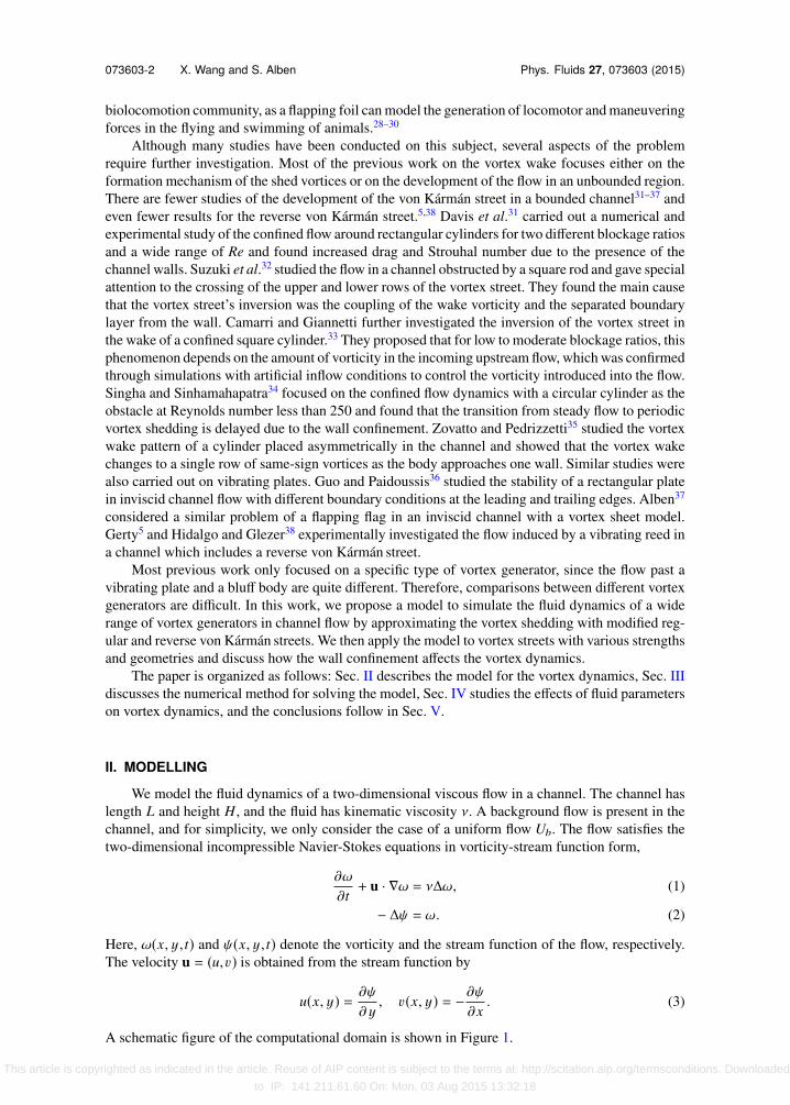
A schematic figure of the computational domain is shown in Figure 1.

This article is copyrighted as indicated in the article. Reuse of AIP content is subject to the terms at: http://scitation.aip.org/termsconditions. Downloaded

to IP: 141.211.61.60 On: Mon, 03 Aug 2015 13:32:18

073603-3 X. Wang and S. Alben Phys. Fluids 27, 073603 (2015)

FIG. 1. Schematic of the computational domain with a uniform background flow Ub. The channel has length L and heightH . Dirichlet boundary conditions are applied at the entrance of the channel. No-penetration and no-slip conditions are usedat the walls and advective derivative conditions are applied to both ω and ψ at the outflow.

A. Boundary conditions

To solve the Navier-Stokes equations, we need to impose proper boundary conditions for ω andψ on each boundary. We discretize the channel with an N × M uniform spatial grid which has Npoints in the x direction and M points in the y direction. The indices (1,1), (N,1), (M,N), and (1,M)indicate the lower left, lower right, upper right, and upper left corners of the computational domain,respectively.

No-slip (u = 0) and no-penetration (v = 0) conditions are applied at the upper and lower wallboundaries of the channel. Both conditions involveψ, while neither involves the vorticityω. To obtaina boundary condition forω, Briley39 proposed a fourth-order formula for the vorticity boundary valuesby using the near-boundary stream function values,

ωi,1 =1

18h2 (85ψi,1 − 108ψi,2 + 27ψi,3 − 4ψi,4) ≡ ωBi,1, ∀i = 1,2, . . . ,N, (4)

ωi,M =1

18h2 (85ψi,M − 108ψi,M−1 + 27ψi,M−2 − 4ψi,M−3) ≡ ωBi,M, ∀i = 1,2, . . . ,N. (5)

Here, h = 1/(M − 1) denotes the grid spacing in the y direction. Briley’s formula is obtained bydiscretizing the no-slip condition ∂ψ/∂ y = 0 with a fourth-order finite difference approximation andthen applying it to Equation (2). The advantage of using a fourth-order instead of a second-orderformula on wall boundaries was discussed by Napolitano40 as he reported smaller global errors intwo numerical examples when using a high-order scheme. The no-penetration condition ∂ψ/∂x = 0gives a Dirichlet boundary condition for ψ,

ψi,1 = ψ1,1, ψi,M = ψ1,M, i = 1,2, . . . ,N, (6)

where ψ1,1 and ψ1,M are the values of ψ at the inflow boundaries, to be given later.Outflow boundary conditions are used to approximate conditions at the channel exit. If the flow

is laminar and the channel is sufficiently long, the flow approaches a Poiseuille flow at the exit, inwhich case the natural boundary condition is a reasonable choice,41,42

∂nω = 0, ∂nψ = 0, (7)

where n is the outward normal coordinate at the exit. This implies that the vertical velocity is zero atthe exit, which is true for Poiseuille flow. However, when the channel is not very long, the flow canstill be transient at the exit, and conditions based on unsteady problems are required. Much previouswork has been carried out on the proper outflow conditions in this case.42–45 In this work, we apply theadvective derivative condition46–48 for ω and ψ at the outflow boundary. Sani and Gresho48 proposedthis condition for the velocity variables,

∂u∂t+ c

∂u∂n= 0, (8)

where c is an average outflow velocity (for example, the averaged streamwise velocity across the exit,u48). Later, Comini and Manzan47 derived conditions for ω and ψ based on Equation (8),

This article is copyrighted as indicated in the article. Reuse of AIP content is subject to the terms at: http://scitation.aip.org/termsconditions. Downloaded

to IP: 141.211.61.60 On: Mon, 03 Aug 2015 13:32:18

073603-4 X. Wang and S. Alben Phys. Fluids 27, 073603 (2015)

∂ω

∂t+ u

∂ω

∂n= 0, (9)

∂

∂t

(∂ψ

∂x

)+ u

(−∂

2ψ

∂y2 − ω)= 0. (10)

Equation (10) is numerically solvable at the exit by combining the wall values of ψ, from the pre-scribed inflow (discussed next), with the no-penetration condition. The advantage of this conditionis that the numerical error caused by truncating the finite domain only affects a local region close tothe exit and does not cause flow disturbances further upstream.48 In this work, we choose L = 4H forthe simulations. This is a moderate length which allows enough flow development without excessivecomputational cost.

Finally, we discuss the inflow boundary conditions. We want to approximate situations wherea vortex generator is placed in front of the channel so that vortices are created and driven into thechannel by an imposed background flow. We model the wakes of such vortex generators as modifiedreverse or regular von Kármán vortex streets with various geometries and strengths.

In inviscid flow, the complex potential of a von Kármán point vortex street is7,49

wvk = φvk + iψvk =iΓ2π

log(sin

π

a(z − z0)

)− iΓ

2πlog

(sin

π

a

(z − z0 −

12

a − ib)), (11)

and the corresponding complex velocity is

uvk = u(z) − iv(z) = iΓ2a

cot(π

a(z − z0)

)− iΓ

2acot

(π

a

(z − z0 −

12

a − ib)), (12)

where point vortices with strength Γ are placed at z0 + (m + 12 )a + ib and those with strength −Γ are

placed at z0 + ma,m = 0,±1,±2, . . . . Positive Γ gives a reverse von Kármán street, while negative Γgives a regular von Kármán street. Equation (12) has a singularity ∼1/z at the point vortex location.However, the point vortex itself travels with a finite velocity because it does not induce velocity at itsown location.7,49 The velocity at z = z0 is

Up =Γ

2atanh

πba. (13)

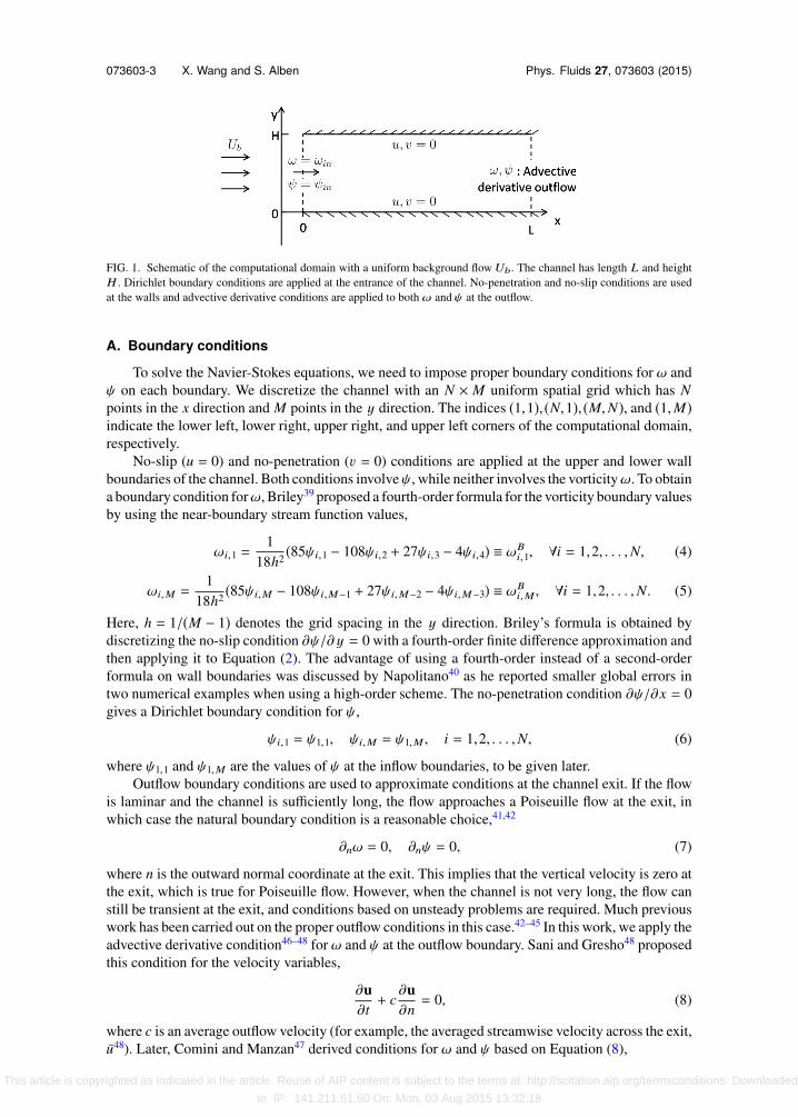
By symmetry, each vortex moves with the same velocity Up.To obtain a more realistic inflow at moderate Reynolds number, we replace the point vortices

in Equation (12) by finite-size vortices, or “vortex blobs,” to account for viscous diffusion. The blobhas radius δ, and the velocity inside the blob is computed by subtracting the point-vortex singularityfrom the von Kármán street solution and adding a desingularized kernel. The complex velocity, thestream function, and the vorticity inside the mth blob are defined as

ublob = uvk(z) − iΓ2π

1z − zm

+iΓ2π

z − zm|z − zm|2 + δ2 , (14)

ψblob = ψvk +Γ

2πlog(|z − zm|) − Γ2π log(

|z − zm|2 + δ2), (15)

ωblob =Γδ2

π(|z − zm|2 + δ2)2 . (16)

Here, the subscript “vk” denotes the von Kármán street solution, and zm is the location of the mthblob. The δ-term is an artificial smoothing kernel that regularizes the point vortex. It is analogous tothe desingularized kernel used by Krasny,50 and as δ → 0, the velocity tends to that of a point vortexmodel. In the region 2δ away from the vortex blob center, we use the velocity of the unmodified pointvortex von Kármán street. A cubic Hermite interpolation (denoted by subscript “herm”) is used toobtain a smooth transition between the two different velocity fields,

u(z) − iv(z) =

uvk(z), |z − zm| > 2δ,uherm, δ < |z − zm| ≤ 2δ,ublob, 0 < |z − zm| ≤ δ.

(17)

This article is copyrighted as indicated in the article. Reuse of AIP content is subject to the terms at: http://scitation.aip.org/termsconditions. Downloaded

to IP: 141.211.61.60 On: Mon, 03 Aug 2015 13:32:18

073603-5 X. Wang and S. Alben Phys. Fluids 27, 073603 (2015)

FIG. 2. (a) A schematic figure of the vortex blob model. The horizontal and vertical displacements between adjacent blobsare 1

2a and b, respectively. The blobs have radii δ and are located at z = 14a+ i

12 (H −b) and z = 3

4a+ i12 (H +b); (b)

cross-sectional values of u at x = 14a and x = 3

4a, with Ub = 1, Γ= 1, and δ = 0.05. The circles indicate the centers ofthe vortex blobs.

The vortex blobs move with the same velocity as in the point vortex case since the blob does notcontribute to its own velocity and the contributions of all the other blobs are the same as in the pointvortex model as they are more than 2δ away. Thus, the vortex blob with an additional uniform back-ground flow Ub has speed

U = Ub +Γ

2atanh

πba. (18)

A schematic figure of the vortex blob model and values of the horizontal velocity u on cross sec-tions through the blob centers for Ub = 1, Γ = 1, a/H = 1, and b/H = 0.5 are shown in Figures 2(a)and 2(b), respectively.

The inflow just described is periodic in x (with period a) and time (with period τp = a/U). Itis a good approximation of the formation of the vortex street when the vorticity has only diffusedslightly. In the numerical simulation, we pre-compute the values of the velocities, vorticity, and streamfunction over one period at the upstream boundary, and then at each time instant t, we impose theappropriate values at t as ω = ωin,ψ = ψin,u = uin, and v = vin.

We summarize all the boundary conditions for fluid Equations (1) and (2),

ω = ωin, ψ = ψin, x = 0,0 < y < H, (19)

∂ω

∂t+ u

∂ω

∂x= 0,

∂

∂t

(∂ψ

∂x

)+ u

(−∂

2ψ

∂y2 − ω)= 0, x = L,0 < y < H, (20)

ω = ωB1 , ψ = ψ1,1, 0 ≤ x ≤ L, y = 0, (21)

ω = ωBM, ψ = ψ1,M, 0 ≤ x ≤ L, y = H, (22)

where ψ1,1 and ψ1,M are obtained from ψin.

B. Nondimensionalization

We classify our flows as either vortex-dominated or background-flow-dominated based on theincoming vortex street conditions. When the strength of the vortex blob |Γ| is larger than the back-ground flow |UbH |, we define the flow as vortex-dominated. Otherwise, the flow is background-flow-dominated. This criterion is applied for both the reverse and regular von Kármán streets.

For simplicity, we use the original notation to indicate all the dimensionless variables. Then,Equations (1)–(3) become

This article is copyrighted as indicated in the article. Reuse of AIP content is subject to the terms at: http://scitation.aip.org/termsconditions. Downloaded

to IP: 141.211.61.60 On: Mon, 03 Aug 2015 13:32:18

073603-6 X. Wang and S. Alben Phys. Fluids 27, 073603 (2015)

∂ω

∂t+ u · ∇ω = 1

Re∆ω, (23)

− ∆ψ = ω, (24)

u =∂ψ

∂ y, v = −∂ψ

∂x, (25)

with several important dimensionless parameters:

1. Sb =bH

, the dimensionless vertical distance between the two rows of vortices.

2. Sa =aH

, the dimensionless horizontal period length.

For the vortex-dominated regime, we choose |Γ|/H as the characteristic velocity, and the dimension-less parameters also include:

3. Re = |Γ|ν , the Reynolds number.

4. Ur =UbH|Γ| , dimensionless background flow.

For the background-flow-dominated regime, we choose Ub as the characteristic velocity, and theparameters include:

3. Re = UbHν , the Reynolds number.

4. Γr =Γ

UbH , dimensionless vortex strength.

Γr can be positive or negative depending on the inflow vortex street type. By definition, Ur and |Γr |are less than or equal to 1. Multiple Reynolds numbers have also been used to describe flows inducedby cylinders51 and flapping bodies.52

In experiments, it would be difficult to control all the parameters (Γ,Ub,Sa,Sb) independentlyas we described in the vortex-blob model. A series of work has been conducted on the relationshipsbetween those parameters, and experimental data and empirical results have provided some typicalvalues for them. Here, we discuss two ways of generating vortex streets and show how to computethe vortex street parameters of our model from experimental measurements.

The regular von Kármán street can be generated by flow past a circular cylinder. In this case,the far-field flow velocity U∞ and the cylinder’s diameter D are the two main control parameters inthe experiments, and the vortex street can be altered by changing these two quantities. For instance,the vertical spacing between the vortices b can be approximated by the diameter D.53,54 The ratioof the vertical to horizontal spacing b/a = Sb/Sa is around 0.28 given by the von Kármán instabilityanalysis53 and around 0.26 by Kronauer’s instability analysis.54 The strength of the vortices is pre-dicted in the work of Berger and Wille55 as Γ ≈ 0.395U∞D/St for flow past a circular cylinder at lowReynolds numbers (less than 200) where St is the Strouhal number. The value of St depends on theReynolds number and ranges between 0.1 and 0.2 for a large range of Re.56 Then, the vortex strengthis approximately 2U∞D to 4U∞D. The velocity of the vortex blob U is approximately 0.89U∞ atRe ≈ 20 000 according to Bearman.57 Therefore, given the values of a,b, Γ, and U∞, the prescribed

background flow can be obtained by Ub = U − Γ2a

tanhπba

.A reverse von Kármán street can be generated by a heaving rigid foil. In this case, the vortices’

shedding frequency f , the far-field flow velocity U∞, and the heaving amplitude A are the main controlparameters in the experiments. In one setup, it was shown that these three parameters must satisfy the

relation StA =2 f AU

> 0.18 to ensure the generation of a reverse von Kármán street at the foil’s trailing

edge.18,19 The vertical spacing can be approximated by the amplitude A and the background flow Ub

is close to the far-field velocity U∞. If we ignore the vortex shedding from the leading edge,18 the

circulation of the vortex at the trailing edge can be approximated by Γ ≈ 12π2A2 f 2. Finally, the hori-

zontal spacing can be obtained by solving the following nonlinear equation: a f = Ub +Γ

2atanh

πba

as a defines the period length of the vortex streets.

This article is copyrighted as indicated in the article. Reuse of AIP content is subject to the terms at: http://scitation.aip.org/termsconditions. Downloaded

to IP: 141.211.61.60 On: Mon, 03 Aug 2015 13:32:18

073603-7 X. Wang and S. Alben Phys. Fluids 27, 073603 (2015)

III. NUMERICAL METHODS

We design our numerical scheme to solve Navier-Stokes Equations (23) and (24) accurately andefficiently in the regime of laminar flow. We discretize the equations with an implicit Crank-Nicolsonscheme to avoid the time step constraints of fully explicit schemes for the Navier-Stokes equations58,59

and linearize the nonlinear advection term by a second-order extrapolation from previous time steps,

un+1/2 =32

un − 12

un−1. (26)

At the first step, we use a first-order extrapolation u1/2 = u0 to obtain u1 and then correct the re-sults by taking u1/2 = 1

2 (u0 + u1), which is also a second-order extrapolation. Spatial derivatives arediscretized with a second-order difference scheme except at the channel walls where a fourth-orderBriley’s formula is used.

With the linearization of the advection term,ω and ψ are coupled only through Briley’s formula.If we place the boundary conditions in a specific order in the system of equations, we can decouple thetwo terms with a computational cost of O(N M) and solve them separately (we refer to Appendix Afor more details). This linearization may be expected to cause an instability when dt is large or theflow changes rapidly. However, we find that for most parameters in the region of interest, a time stepof dt = 1/128 is good enough for a stable result.

Since the incoming vortex street is time-periodic, we expect that the channel flow also convergesto a time-periodic solution whose period is that of the incoming flow, given by τp = Sa/U. In thesimulation, we start from zero initial flow and evolve the flow with our time-marching scheme until itconverges to a time-periodic state. The vorticity profiles at the end of each period ωkτp, k = 0,1, . . .are used for comparison, and the simulation is terminated when ∥ωkτp − ω(k−1)τp∥2 ≤ 10−8. We findthat for a grid size of 513 × 129 and dt = 1/128, it generally takes fewer than 30 periods for thechannel flow to become time-periodic starting from zero flow. Convergence studies are performed forsolutions at fixed times. We only obtain a convergence order between 1 and 2 for both time and space,because the problem is singular at the leading edge of the channel and in the initial condition. Forsmooth problems, second-order convergence is obtained for both time and spatial variables. Detailsabout the numerical methods and convergence studies are provided in Appendices A and B.

IV. RESULTS AND DISCUSSION

Now we present the channel flows that result from the two types of incoming flows: reverseand regular von Kármán streets. Unlike flows in an unbounded region, the flow behaves dramaticallydifferent for these two types of incoming flows due to the existence of the walls. We are mainly inter-ested in the periodic-state solutions. Therefore, all the results presented in this section are obtainedby the above numerical method and are in the time-periodic state unless stated.

A. Reverse von Kármán street

In the reverse von Kármán street case, two staggered rows of vortex blobs enter the channelperiodically with positive circulations in the upper row and negative circulations in the lower row.

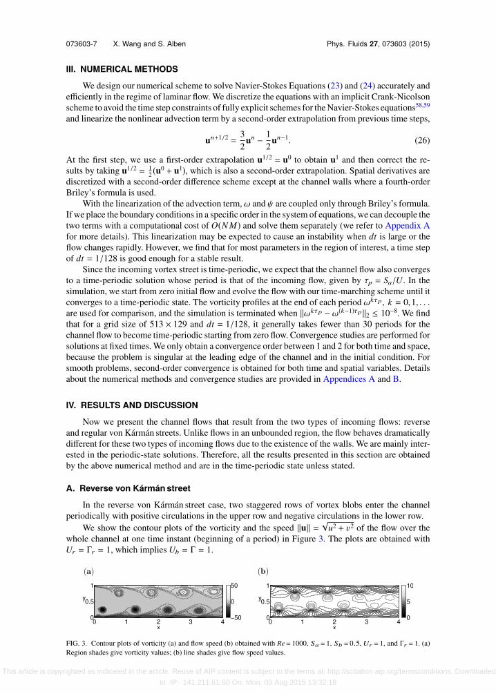
We show the contour plots of the vorticity and the speed ∥u∥ = √u2 + v2 of the flow over thewhole channel at one time instant (beginning of a period) in Figure 3. The plots are obtained withUr = Γr = 1, which implies Ub = Γ = 1.

FIG. 3. Contour plots of vorticity (a) and flow speed (b) obtained with Re= 1000, Sa = 1, Sb = 0.5, Ur = 1, and Γr = 1. (a)Region shades give vorticity values; (b) line shades give flow speed values.

This article is copyrighted as indicated in the article. Reuse of AIP content is subject to the terms at: http://scitation.aip.org/termsconditions. Downloaded

to IP: 141.211.61.60 On: Mon, 03 Aug 2015 13:32:18

073603-8 X. Wang and S. Alben Phys. Fluids 27, 073603 (2015)

FIG. 4. Instantaneous contour plots of vorticity obtained with Sa = 1, Sb = 0.5, Ur = 1, Γr = 1, and (a) Re= 200, (b)Re= 500, (c) Re= 2000, and (d) Re= 5000.

In Figure 3(a), we notice that the vortex blobs mainly move in the downstream direction and thestructure of the reverse von Kármán vortex street is maintained in the channel. The blobs diffuse in thechannel, and their shape approximates a semicircle due to the walls’ presence. Each blob induces anupstream flow between the blob itself and the wall and decreases the speed of the flow in that region,as shown in Figure 3(b). This flow thus generates opposite-signed vorticity in the boundary layeradjacent to the corresponding vortex blob, which leads to alternating positive and negative vorticitiesin the boundary layer.

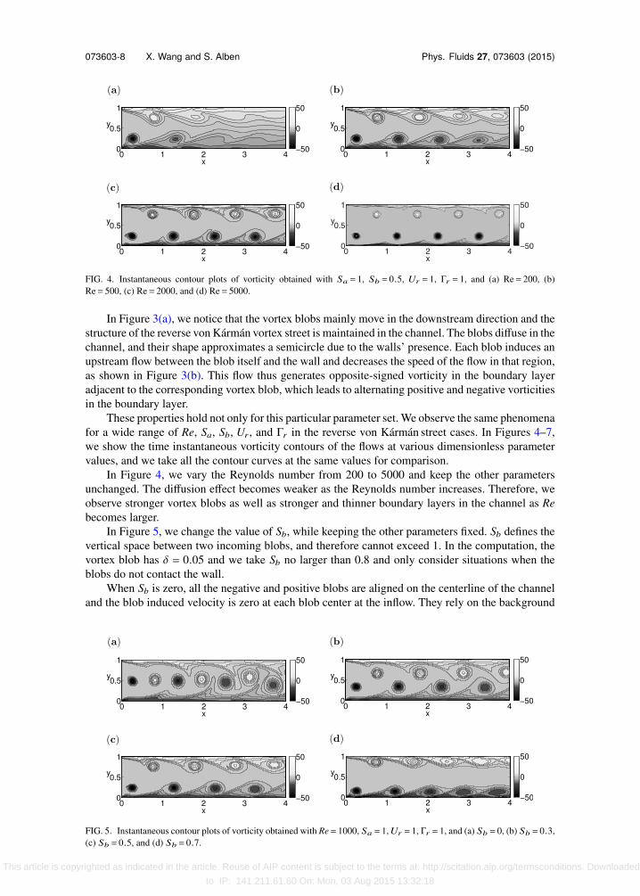
These properties hold not only for this particular parameter set. We observe the same phenomenafor a wide range of Re, Sa, Sb, Ur , and Γr in the reverse von Kármán street cases. In Figures 4–7,we show the time instantaneous vorticity contours of the flows at various dimensionless parametervalues, and we take all the contour curves at the same values for comparison.

In Figure 4, we vary the Reynolds number from 200 to 5000 and keep the other parametersunchanged. The diffusion effect becomes weaker as the Reynolds number increases. Therefore, weobserve stronger vortex blobs as well as stronger and thinner boundary layers in the channel as Rebecomes larger.

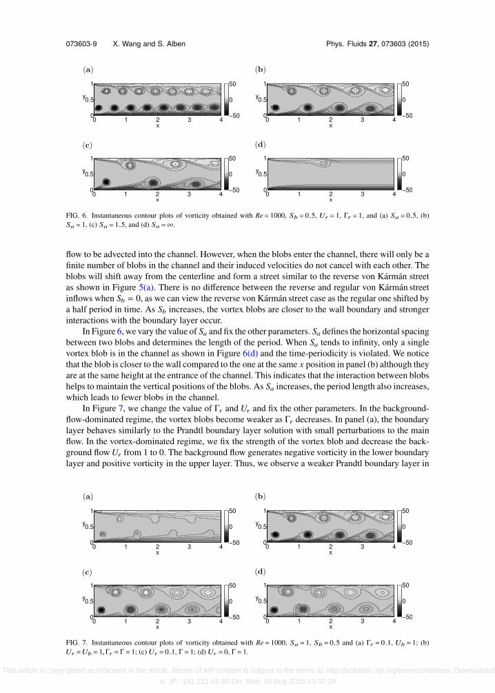
In Figure 5, we change the value of Sb, while keeping the other parameters fixed. Sb defines thevertical space between two incoming blobs, and therefore cannot exceed 1. In the computation, thevortex blob has δ = 0.05 and we take Sb no larger than 0.8 and only consider situations when theblobs do not contact the wall.

When Sb is zero, all the negative and positive blobs are aligned on the centerline of the channeland the blob induced velocity is zero at each blob center at the inflow. They rely on the background

FIG. 5. Instantaneous contour plots of vorticity obtained with Re= 1000, Sa = 1,Ur = 1, Γr = 1, and (a) Sb = 0, (b) Sb = 0.3,(c) Sb = 0.5, and (d) Sb = 0.7.

This article is copyrighted as indicated in the article. Reuse of AIP content is subject to the terms at: http://scitation.aip.org/termsconditions. Downloaded

to IP: 141.211.61.60 On: Mon, 03 Aug 2015 13:32:18

073603-9 X. Wang and S. Alben Phys. Fluids 27, 073603 (2015)

FIG. 6. Instantaneous contour plots of vorticity obtained with Re= 1000, Sb = 0.5, Ur = 1, Γr = 1, and (a) Sa = 0.5, (b)Sa = 1, (c) Sa = 1.5, and (d) Sa =∞.

flow to be advected into the channel. However, when the blobs enter the channel, there will only be afinite number of blobs in the channel and their induced velocities do not cancel with each other. Theblobs will shift away from the centerline and form a street similar to the reverse von Kármán streetas shown in Figure 5(a). There is no difference between the reverse and regular von Kármán streetinflows when Sb = 0, as we can view the reverse von Kármán street case as the regular one shifted bya half period in time. As Sb increases, the vortex blobs are closer to the wall boundary and strongerinteractions with the boundary layer occur.

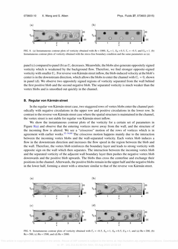
In Figure 6, we vary the value of Sa and fix the other parameters. Sa defines the horizontal spacingbetween two blobs and determines the length of the period. When Sa tends to infinity, only a singlevortex blob is in the channel as shown in Figure 6(d) and the time-periodicity is violated. We noticethat the blob is closer to the wall compared to the one at the same x position in panel (b) although theyare at the same height at the entrance of the channel. This indicates that the interaction between blobshelps to maintain the vertical positions of the blobs. As Sa increases, the period length also increases,which leads to fewer blobs in the channel.

In Figure 7, we change the value of Γr and Ur and fix the other parameters. In the background-flow-dominated regime, the vortex blobs become weaker as Γr decreases. In panel (a), the boundarylayer behaves similarly to the Prandtl boundary layer solution with small perturbations to the mainflow. In the vortex-dominated regime, we fix the strength of the vortex blob and decrease the back-ground flow Ur from 1 to 0. The background flow generates negative vorticity in the lower boundarylayer and positive vorticity in the upper layer. Thus, we observe a weaker Prandtl boundary layer in

FIG. 7. Instantaneous contour plots of vorticity obtained with Re= 1000, Sa = 1, Sb = 0.5 and (a) Γr = 0.1, Ub = 1; (b)Ur =Ub = 1,Γr = Γ= 1; (c) Ur = 0.1, Γ= 1; (d) Ur = 0, Γ= 1.

This article is copyrighted as indicated in the article. Reuse of AIP content is subject to the terms at: http://scitation.aip.org/termsconditions. Downloaded

to IP: 141.211.61.60 On: Mon, 03 Aug 2015 13:32:18

073603-10 X. Wang and S. Alben Phys. Fluids 27, 073603 (2015)

FIG. 8. (a) Instantaneous contour plots of vorticity obtained with Re= 1000, Sa = 1, Sb = 0.5, Γr =−0.5, and Ub = 1. (b)Instantaneous contour plots of vorticity obtained with the stress-free boundary condition and the same parameters as (a).

panel (c) compared to panel (b) as Ur decreases. Meanwhile, the blobs also generate oppositely signedvorticity which is weakened by the background flow. Therefore, we find stronger opposite-signedvorticity with smaller Ur . For reverse von Kármán street inflow, the blob-induced velocity at the blob’scenter is in the downstream direction, which allows the blobs to enter the channel with Ur = 0, shownin panel (d). We observe two oppositely signed regions of vorticity separated from the wall behindthe first positive blob and the second negative blob. The separated vorticity is much weaker than thevortex blobs and is smoothed out quickly in the channel.

B. Regular von Kármán street

In the regular von Kármán street case, two staggered rows of vortex blobs enter the channel peri-odically with negative circulations in the upper row and positive circulations in the lower row. Incontrast to the reverse von Kármán street case where the spatial structure is maintained in the channel,the vortex street is not stable for regular von Kármán street inflow.

We show the instantaneous contour plots of the vorticity for a certain set of parameters inFigure 8(a) and observe that the entering vortices move away from the wall, and the structure ofthe incoming flow is altered. We see a “crisscross” motion of the rows of vortices which is inagreement with earlier works.32–34,60 The crisscross motion happens mainly due to the interactionbetween the incoming vortex blobs and the wall-separated vorticity. Each vortex blob induces aflow in the downstream direction and increases the flow speed in the region between the blob andthe wall. Therefore, the vortex blob reinforces the boundary layer and leads to strong vorticity withopposite sign on the wall which then separates. The interaction between the incoming vortex bloband the separated vorticity of the adjacent wall boundary layer then pushes the negative vortex blobdownwards and the positive blob upwards. The blobs thus cross the centerline and exchange theirpositions in the channel. Afterwards, the positive blobs remain in the upper half and the negative blobsin the lower half, forming a street with a structure similar to that of the reverse von Kármán street.

FIG. 9. Instantaneous contour plots of vorticity obtained with Γr =−0.5, Sa = 1, Sb = 0.5, Ub = 1, and (a) Re= 200, (b)Re= 500, (c) Re= 1500, and (d) Re= 2000.

This article is copyrighted as indicated in the article. Reuse of AIP content is subject to the terms at: http://scitation.aip.org/termsconditions. Downloaded

to IP: 141.211.61.60 On: Mon, 03 Aug 2015 13:32:18

073603-11 X. Wang and S. Alben Phys. Fluids 27, 073603 (2015)

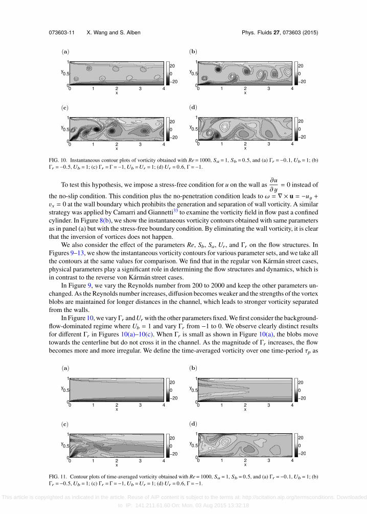
FIG. 10. Instantaneous contour plots of vorticity obtained with Re= 1000, Sa = 1, Sb = 0.5, and (a) Γr =−0.1, Ub = 1; (b)Γr =−0.5, Ub = 1; (c) Γr = Γ=−1, Ub =Ur = 1; (d) Ur = 0.6, Γ=−1.

To test this hypothesis, we impose a stress-free condition for u on the wall as∂u∂ y= 0 instead of

the no-slip condition. This condition plus the no-penetration condition leads to ω = ∇ × u = −uy +vx = 0 at the wall boundary which prohibits the generation and separation of wall vorticity. A similarstrategy was applied by Camarri and Giannetti33 to examine the vorticity field in flow past a confinedcylinder. In Figure 8(b), we show the instantaneous vorticity contours obtained with same parametersas in panel (a) but with the stress-free boundary condition. By eliminating the wall vorticity, it is clearthat the inversion of vortices does not happen.

We also consider the effect of the parameters Re, Sb, Sa, Ur , and Γr on the flow structures. InFigures 9–13, we show the instantaneous vorticity contours for various parameter sets, and we take allthe contours at the same values for comparison. We find that in the regular von Kármán street cases,physical parameters play a significant role in determining the flow structures and dynamics, which isin contrast to the reverse von Kármán street cases.

In Figure 9, we vary the Reynolds number from 200 to 2000 and keep the other parameters un-changed. As the Reynolds number increases, diffusion becomes weaker and the strengths of the vortexblobs are maintained for longer distances in the channel, which leads to stronger vorticity separatedfrom the walls.

In Figure 10, we vary Γr andUr with the other parameters fixed. We first consider the background-flow-dominated regime where Ub = 1 and vary Γr from −1 to 0. We observe clearly distinct resultsfor different Γr in Figures 10(a)–10(c). When Γr is small as shown in Figure 10(a), the blobs movetowards the centerline but do not cross it in the channel. As the magnitude of Γr increases, the flowbecomes more and more irregular. We define the time-averaged vorticity over one time-period τp as

FIG. 11. Contour plots of time-averaged vorticity obtained with Re= 1000, Sa = 1, Sb = 0.5, and (a) Γr =−0.1, Ub = 1; (b)Γr =−0.5, Ub = 1; (c) Γr = Γ=−1, Ub =Ur = 1; (d) Ur = 0.6, Γ=−1.

This article is copyrighted as indicated in the article. Reuse of AIP content is subject to the terms at: http://scitation.aip.org/termsconditions. Downloaded

to IP: 141.211.61.60 On: Mon, 03 Aug 2015 13:32:18

073603-12 X. Wang and S. Alben Phys. Fluids 27, 073603 (2015)

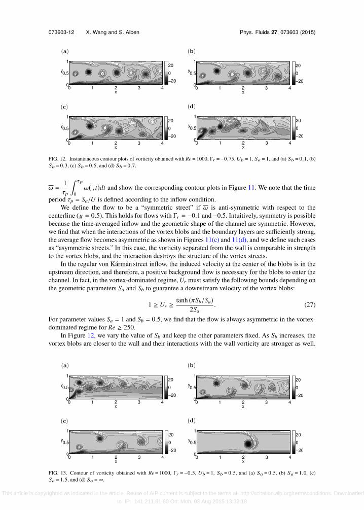
FIG. 12. Instantaneous contour plots of vorticity obtained with Re= 1000, Γr =−0.75, Ub = 1, Sa = 1, and (a) Sb = 0.1, (b)Sb = 0.3, (c) Sb = 0.5, and (d) Sb = 0.7.

ω =1τp

τp

0ω(·, t)dt and show the corresponding contour plots in Figure 11. We note that the time

period τp = Sa/U is defined according to the inflow condition.We define the flow to be a “symmetric street” if ω is anti-symmetric with respect to the

centerline (y = 0.5). This holds for flows with Γr = −0.1 and −0.5. Intuitively, symmetry is possiblebecause the time-averaged inflow and the geometric shape of the channel are symmetric. However,we find that when the interactions of the vortex blobs and the boundary layers are sufficiently strong,the average flow becomes asymmetric as shown in Figures 11(c) and 11(d), and we define such casesas “asymmetric streets.” In this case, the vorticity separated from the wall is comparable in strengthto the vortex blobs, and the interaction destroys the structure of the vortex streets.

In the regular von Kármán street inflow, the induced velocity at the center of the blobs is in theupstream direction, and therefore, a positive background flow is necessary for the blobs to enter thechannel. In fact, in the vortex-dominated regime, Ur must satisfy the following bounds depending onthe geometric parameters Sa and Sb to guarantee a downstream velocity of the vortex blobs:

1 ≥ Ur ≥tanh (πSb/Sa)

2Sa. (27)

For parameter values Sa = 1 and Sb = 0.5, we find that the flow is always asymmetric in the vortex-dominated regime for Re ≥ 250.

In Figure 12, we vary the value of Sb and keep the other parameters fixed. As Sb increases, thevortex blobs are closer to the wall and their interactions with the wall vorticity are stronger as well.

FIG. 13. Contour of vorticity obtained with Re= 1000, Γr =−0.5, Ub = 1, Sb = 0.5, and (a) Sa = 0.5, (b) Sa = 1.0, (c)Sa = 1.5, and (d) Sa =∞.

This article is copyrighted as indicated in the article. Reuse of AIP content is subject to the terms at: http://scitation.aip.org/termsconditions. Downloaded

to IP: 141.211.61.60 On: Mon, 03 Aug 2015 13:32:18

073603-13 X. Wang and S. Alben Phys. Fluids 27, 073603 (2015)

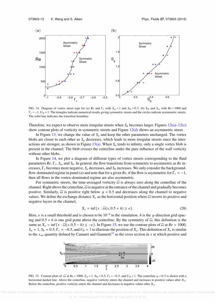
FIG. 14. Diagram of vortex street type for (a) Re and Γr with Sa = 1 and Sb = 0.5. (b) Sb and Sa with Re= 1000 andΓr =−1,Ub = 1. The triangles indicate numerical results giving symmetric streets and the circles indicate asymmetric streets.The solid line indicates the transition boundary.

Therefore, we expect to observe more irregular streets when Sb becomes larger. Figures 12(a)–12(c)show contour plots of vorticity in symmetric streets and Figure 12(d) shows an asymmetric street.

In Figure 13, we change the value of Sa and keep the other parameters unchanged. The vortexblobs are closer to each other as Sa decreases, which leads to more irregular streets since the inter-actions are stronger, as shown in Figure 13(a). When Sa tends to infinity, only a single vortex blob ispresent in the channel. The blob crosses the centerline under the pure influence of the wall vorticitywithout other blobs.

In Figure 14, we plot a diagram of different types of vortex streets corresponding to the fluidparameters Re, Γr , Sa, and Sb. In general, the flow transitions from symmetric to asymmetric as Re in-creases, Γr becomes more negative, Sa decreases, and Sb increases. We only consider the background-flow-dominated regime in panel (a) and note that for a given Re, if the flow is asymmetric for Γr = −1,then all flows in the vortex-dominated regime are also asymmetric.

For symmetric streets, the time-averaged vorticity ω is always zero along the centerline of thechannel. Right above the centerline,ω is negative at the entrance of the channel and gradually becomespositive. Similarly, ω is positive right below y = 0.5 and decreases along the channel to negativevalues. We define the exchange distance Xe as the horizontal position whereω inverts its positive andnegative layers in the channel,

Xe = inf{x : ω(x,0.5 + h) ≥ ϵ}. (28)

Here, ϵ is a small threshold and is chosen to be 10−6 in the simulation. h is the y-direction grid spac-ing and 0.5 + h is one grid point above the centerline. By the symmetry of ω, this definition is thesame as Xe = inf{x : ω(x,0.5 − h) ≤ −ϵ}. In Figure 15, we use the contour plots ofω at Re = 1000,Sa = 1, Sb = 0.5, Γr = −0.5, and Ub = 1 to illustrate the position of Xe. This definition of Xe is similarto the xinv quantity defined by Camarri and Giannetti33 as the cross section in x at which positive and

FIG. 15. Contour plots of ω at Re= 1000, Sa = 1, Sb = 0.5, Γr =−0.5, and Ub = 1. The centerline y = 0.5 is shown with ahorizontal dashed line. Above the centerline, negative vorticity enters the channel and increases to positive values after Xe.Below the centerline, positive vorticity enters the channel and decreases to negative values after Xe.

This article is copyrighted as indicated in the article. Reuse of AIP content is subject to the terms at: http://scitation.aip.org/termsconditions. Downloaded

to IP: 141.211.61.60 On: Mon, 03 Aug 2015 13:32:18

073603-14 X. Wang and S. Alben Phys. Fluids 27, 073603 (2015)

FIG. 16. (a) Xe vs. Re with Γr =−0.2,−0.3,−0.4,−0.5,−0.6,−0.7,−0.8,Ub = 1, Sa = 1, and Sb = 0.5; (b) Xe vs. Sb withSa = 1,1.25,1.5,1.75,2, Γr =−0.75, Ub = 1, and Re= 1000.

negative vortex trajectories intersect. Xe depends on Re, Γr , Sb, and Sa, and we plot Xe versus differentparameters in Figure 16. We only consider Xe for symmetric streets. The missing data points in thegraph indicate that the street is asymmetric for that particular parameter set. We define Xe = 4 if thepositive and negative blobs do not cross the centerline in the channel.

In panel (a), we find that Xe increases when the Reynolds number increases. This is in contrast tothe observation by Camarri et al.33 where they found the inverted position monotonically decreaseswith Re. However, their work focuses on a narrower range of Reynolds numbers (50-170) with asquare cylinder as the vortex generator, which is different from our model. When Γr becomes morenegative, the vortex blobs and the interactions with the separated vorticity are stronger, resulting ina smaller exchange distance.

When Sb increases, the blobs are closer to the wall which makes them move towards the center-line faster, as the wall interactions are stronger. On the other hand, the blobs must also travel furtherto invert their positions as they are further moved from the centerline. Therefore, in panel (b), themaximum Xe is obtained at a moderate value of Sb instead of at the boundaries, and we find that Xe

decays linearly with Sb beyond the maximum.The effect of Sa on Xe is also complicated. When Sb < 0.175, we notice that Xe decreases with

Sa, and when Sb ≥ 0.2, it increases with Sa. When Sb is sufficiently small and the blob is close to thecenterline, the inversion location mainly depends on the speed of the vortex blob. For negative Γr , thisspeed increases with Sa which leads to smaller Xe. When Sb is large, the blobs are pushed towards thecenterline through their interactions with the boundary vorticity. The exchange distance Xe is moreinfluenced by the strength of these interactions. We therefore observe smaller Xe with smaller Sa asthe interactions between the blobs and the separated vorticity are stronger.

V. CONCLUSION

In this work, we have numerically studied the effect of wall confinement on vortex street dy-namics in a channel flow. Instead of modelling a specific vortex generator, we model typical wakesas smoothed von Kármán vortex streets with various vortex strengths and geometries and apply themas inflow boundary conditions. This approximation allows us to explore a large parameter space of{Re,Γr ,Ur ,Sb,Sa} and classify the vortex dynamics of the channel flows.

When the inflow is a reverse von Kármán street, we find that vortex blobs maintain their spatialstructure from the inflow and mainly move in the downstream direction. When the inflow is a regularvon Kármán street, we find that the vortex blobs move towards the centerline and exchange theirpositions in the channel. This “criss-cross” motion is due to the interactions between the blobs and theseparated vorticity from the wall. The location where the inversion happens depends on the strength ofthis interaction, as well as the momentum of the vortex blobs and the geometry of the incoming streets.

This article is copyrighted as indicated in the article. Reuse of AIP content is subject to the terms at: http://scitation.aip.org/termsconditions. Downloaded

to IP: 141.211.61.60 On: Mon, 03 Aug 2015 13:32:18

073603-15 X. Wang and S. Alben Phys. Fluids 27, 073603 (2015)

For the regular von Kármán streets, different parameters lead to very different flow profiles. Wehave classified them as symmetric or asymmetric streets depending on the symmetry of the time-averaged vorticity. The transition to asymmetry happens when the interactions between the blobsand the separated vorticity are sufficiently strong to destroy the spatial structure of the inflow. Wehave determined the transition location in certain cross sections of {Re,Γr ,Sb,Sa} space. In general,the flow transitions to asymmetric as Re increases, Γr becomes more negative, Sa decreases, and Sbincreases.

An extension of this work is to consider the vortex dynamics in a three-dimensional channel.This requires an understanding of the vortex wakes behind different vortex generators in 3-D flow.Another interesting topic is to apply the current fluid model to study the vorticity-enhanced heattransfer process. For example, Hildago et al.61 used a piezoelectric driven reed to generate a reversevon Kármán street in a heated channel and found a large increase in the coefficient of performance(the ratio of the thermal power dissipation to the mechanical power used to drive the flow). Shoeleand Mittal62 studied heat transfer of a self-oscillating flexible reed in a channel flow which generateda regular von Kármán vortex wake. They reported that the optimal thermal performance is achievedwhen the vortex wake disrupts the boundary layer but does not have strong vortices. A better under-standing of the vortex dynamics in a channel flow may suggest vortex generators with improvedthermal performance.

ACKNOWLEDGMENTS

We acknowledge support from NSF-DMS, Grant No. 1329726 and a Sloan Research Fellowship(S.A.).

APPENDIX A: NUMERICAL METHODS

In this section, we show the details of our numerical methods. Equations (23) and (24) are dis-cretized with an linearized implicit Crank-Nicolson scheme. Denoting the current time step as n, thetime discretization is

ωn+1 − ωn

dt+

12

un+1/2 · (∇ωn+1 + ∇ωn) = 12

1Re

(∆ωn+1 + ∆ωn), (A1)

−∆ψn+1 = ωn+1. (A2)

With the linearization of the advection term, we see that Equations (A1) and (A2) are coupledonly through Briley’s formula and if we place the boundary conditions in a specific order in the systemof equations, we can write the linear system as follows:

This article is copyrighted as indicated in the article. Reuse of AIP content is subject to the terms at: http://scitation.aip.org/termsconditions. Downloaded

to IP: 141.211.61.60 On: Mon, 03 Aug 2015 13:32:18

073603-16 X. Wang and S. Alben Phys. Fluids 27, 073603 (2015)

Here, B stands for Briley’s formula, L = −∆ + u · ∇, c = −dt u, adv . denotes the advective deriv-ative condition, I(ωin) and I(ψin) are the identity matrices from the inflow conditions onω and ψ, andI(ψw) is the identity matrix from the wall boundary condition on ψ. The linear system can be writtenin block matrix form as

*,

A11 A12

A21 A22

+-*,

ψ

ω+-= *,

b1

b2

+-. (A3)

The problem can be solved by a block LU decomposition which leads to the linear system,

(A21 − A22A−112 A11)ψ = b2 − A22A−1

12 b1. (A4)

The matrix in Equation (A4) can be formed explicitly as all four blocks are sparse matrices andthe right-upper block A12 is a diagonal matrix given u , 0. A21 has only 2N + M + 1 nonzeros onthe diagonal, and both A11 and A22 are close to pentadiagonal matrices except at boundary points.The computational cost to explicitly form the matrix in Equation (A4) is O(N M). The linear matrixcan be solved by an iterative method such GMRES with a preconditioner.63,64 However, we find adirect solver is sufficiently fast and scalable. For a spatial grid of 513 × 129 and dt = 1/128, it takesabout 150 s to run the simulation for one period on a single processor. The computational cost scalesapproximately as (N M)1.3.

Once ψ is obtained, we obtain ω by the following equation:

ω = A−112 b1 − A−1

12 A11ψ. (A5)

Since A12 is a diagonal matrix, only matrix-vector multiplication is required to obtain ω from ψ.

APPENDIX B: CONVERGENCE STUDY

In this section, we display the results of convergence studies for time and space. For a smoothproblem, second order convergence is expected for both time and spatial variables. For all the numer-ical results obtained here, we use the following parameters: the length of the channel L = 4, the heightof the channel H = 1, Sa = 1, and Sb = 0.5. We choose Ub = Γ = 1 for the reverse von Kármán streetsand Ub = 1,Γ = −0.5 for regular von Kármán street, and Re = 500 for both cases.

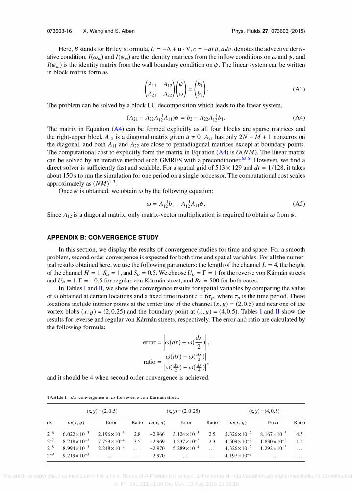
In Tables I and II, we show the convergence results for spatial variables by comparing the valueof ω obtained at certain locations and a fixed time instant t = 6τp, where τp is the time period. Theselocations include interior points at the center line of the channel (x, y) = (2,0.5) and near one of thevortex blobs (x, y) = (2,0.25) and the boundary point at (x, y) = (4,0.5). Tables I and II show theresults for reverse and regular von Kármán streets, respectively. The error and ratio are calculated bythe following formula:

error =�����ω(dx) − ω(dx

2)�����,

ratio =

�ω(dx) − ω( dx2 )��ω( dx2 ) − ω( dx4 )� ,

and it should be 4 when second order convergence is achieved.

TABLE I. dx-convergence in ω for reverse von Kármán street.

(x,y)= (2,0.5) (x,y)= (2,0.25) (x,y)= (4,0.5)dx ω(x, y) Error Ratio ω(x, y) Error Ratio ω(x, y) Error Ratio

2−6 6.022×10−3 2.196×10−3 2.8 −2.966 3.124×10−3 2.5 5.326×10−2 8.167×10−3 4.52−7 8.218×10−3 7.759×10−4 3.5 −2.969 1.237×10−3 2.3 4.509×10−2 1.830×10−3 1.42−8 8.994×10−3 2.248×10−4 . . . −2.970 5.289×10−4 . . . 4.326×10−2 1.292×10−3 . . .2−9 9.219×10−3 . . . . . . −2.970 . . . . . . 4.197×10−2 . . . . . .

This article is copyrighted as indicated in the article. Reuse of AIP content is subject to the terms at: http://scitation.aip.org/termsconditions. Downloaded

to IP: 141.211.61.60 On: Mon, 03 Aug 2015 13:32:18

073603-17 X. Wang and S. Alben Phys. Fluids 27, 073603 (2015)

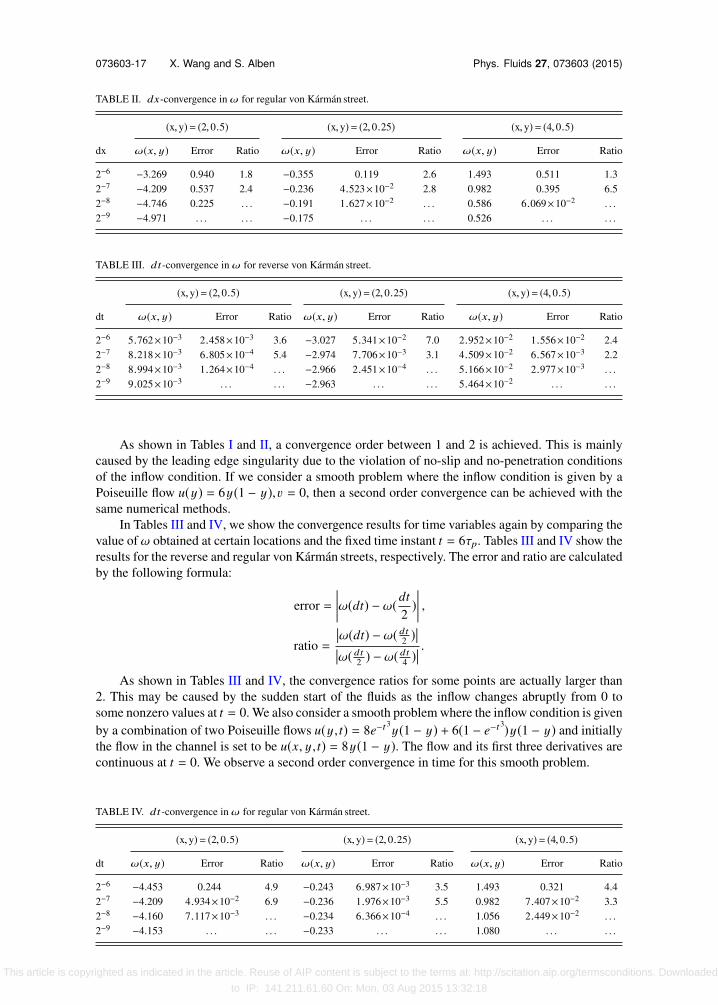
TABLE II. dx-convergence in ω for regular von Kármán street.

(x,y)= (2,0.5) (x,y)= (2,0.25) (x,y)= (4,0.5)dx ω(x, y) Error Ratio ω(x, y) Error Ratio ω(x, y) Error Ratio

2−6 −3.269 0.940 1.8 −0.355 0.119 2.6 1.493 0.511 1.32−7 −4.209 0.537 2.4 −0.236 4.523×10−2 2.8 0.982 0.395 6.52−8 −4.746 0.225 . . . −0.191 1.627×10−2 . . . 0.586 6.069×10−2 . . .2−9 −4.971 . . . . . . −0.175 . . . . . . 0.526 . . . . . .

TABLE III. dt-convergence in ω for reverse von Kármán street.

(x,y)= (2,0.5) (x,y)= (2,0.25) (x,y)= (4,0.5)dt ω(x, y) Error Ratio ω(x, y) Error Ratio ω(x, y) Error Ratio

2−6 5.762×10−3 2.458×10−3 3.6 −3.027 5.341×10−2 7.0 2.952×10−2 1.556×10−2 2.42−7 8.218×10−3 6.805×10−4 5.4 −2.974 7.706×10−3 3.1 4.509×10−2 6.567×10−3 2.22−8 8.994×10−3 1.264×10−4 . . . −2.966 2.451×10−4 . . . 5.166×10−2 2.977×10−3 . . .2−9 9.025×10−3 . . . . . . −2.963 . . . . . . 5.464×10−2 . . . . . .

As shown in Tables I and II, a convergence order between 1 and 2 is achieved. This is mainlycaused by the leading edge singularity due to the violation of no-slip and no-penetration conditionsof the inflow condition. If we consider a smooth problem where the inflow condition is given by aPoiseuille flow u(y) = 6y(1 − y), v = 0, then a second order convergence can be achieved with thesame numerical methods.

In Tables III and IV, we show the convergence results for time variables again by comparing thevalue ofω obtained at certain locations and the fixed time instant t = 6τp. Tables III and IV show theresults for the reverse and regular von Kármán streets, respectively. The error and ratio are calculatedby the following formula:

error =�����ω(dt) − ω(dt

2)�����,

ratio =

�ω(dt) − ω( dt2 )��ω( dt2 ) − ω( dt4 )� .

As shown in Tables III and IV, the convergence ratios for some points are actually larger than2. This may be caused by the sudden start of the fluids as the inflow changes abruptly from 0 tosome nonzero values at t = 0. We also consider a smooth problem where the inflow condition is givenby a combination of two Poiseuille flows u(y, t) = 8e−t

3y(1 − y) + 6(1 − e−t

3)y(1 − y) and initiallythe flow in the channel is set to be u(x, y, t) = 8y(1 − y). The flow and its first three derivatives arecontinuous at t = 0. We observe a second order convergence in time for this smooth problem.

TABLE IV. dt-convergence in ω for regular von Kármán street.

(x,y)= (2,0.5) (x,y)= (2,0.25) (x,y)= (4,0.5)dt ω(x, y) Error Ratio ω(x, y) Error Ratio ω(x, y) Error Ratio

2−6 −4.453 0.244 4.9 −0.243 6.987×10−3 3.5 1.493 0.321 4.42−7 −4.209 4.934×10−2 6.9 −0.236 1.976×10−3 5.5 0.982 7.407×10−2 3.32−8 −4.160 7.117×10−3 . . . −0.234 6.366×10−4 . . . 1.056 2.449×10−2 . . .2−9 −4.153 . . . . . . −0.233 . . . . . . 1.080 . . . . . .

This article is copyrighted as indicated in the article. Reuse of AIP content is subject to the terms at: http://scitation.aip.org/termsconditions. Downloaded

to IP: 141.211.61.60 On: Mon, 03 Aug 2015 13:32:18

073603-18 X. Wang and S. Alben Phys. Fluids 27, 073603 (2015)

1 A. M. Jacobi and R. K. Shah, “Heat transfer surface enhancement through the use of longitudinal vortices: A review ofrecent progress,” Exp. Therm. Fluid Sci. 11(3), 295–309 (1995).

2 J. G. Li, “A mechanism for heat transfer enhancements by vortex shedding,” in Fluids Engineering Division Conference,FED, San Diego, California (ASME, 1996), Vol. 239, p. 533.

3 M. Fiebig, P. Kallweit, N. Mitra, and S. Tiggelbeck, “Heat transfer enhancement and drag by longitudinal vortex generatorsin channel flow,” Exp. Therm. Fluid Sci. 4(1), 103–114 (1991).

4 T. Açıkalın, S. V. Garimella, A. Raman, and J. Petroski, “Characterization and optimization of the thermal performance ofminiature piezoelectric fans,” Int. J. Heat Fluid Flow 28(4), 806–820 (2007).

5 D. Gerty, “Fluidic-driven cooling of electronic hardware,” Ph.D. dissertation, Georgia Institute of Technology, 2008.6 A. Sharma and V. Eswaran, “Heat and fluid flow across a square cylinder in the two-dimensional laminar flow regime,”

Numer. Heat Transfer, Part A 45(3), 247–269 (2004).7 P. G. Saffman, Vortex Dynamics (Cambridge Univ. Press, 1992).8 T. Sarpkaya and R. L. Schoaff, “Inviscid model of two-dimensional vortex shedding by a circular cylinder,” AIAA J. 17(11),

1193–1200 (1979).9 R. R. Clements, “An inviscid model of two-dimensional vortex shedding,” J. Fluid Mech. 57(2), 321–336 (1973).

10 M. Kiya and M. Arie, “A contribution to an inviscid vortex-shedding model for an inclined flat plate in uniform flow,”J. Fluid Mech. 82(2), 223–240 (1977).

11 J. H. Gerrard, “The mechanics of the formation region of vortices behind bluff bodies,” J. Fluid Mech. 25(02), 401–413(1966).

12 S. Tang and N. Aubry, “On the symmetry breaking instability leading to vortex shedding,” Phys. Fluids 9(9), 2550–2561(1997).

13 A. E. Perry, M. S. Chong, and T. T. Lim, “The vortex-shedding process behind two-dimensional bluff bodies,” J. Fluid Mech.116, 77–90 (1982).

14 H. Oertel, Jr., “Wakes behind blunt bodies,” Annu. Rev. Fluid Mech. 22(1), 539–562 (1990).15 C. H. K. Williamson, “Vortex dynamics in the cylinder wake,” Annu. Rev. Fluid Mech. 28(1), 477–539 (1996).16 A. Kumar De and A. Dalal, “Numerical simulation of unconfined flow past a triangular cylinder,” Int. J. Numer. Methods

Fluids 52(7), 801–821 (2006).17 M. M. Koochesfahani, “Vortical patterns in the wake of an oscillating airfoil,” AIAA J. 27(9), 1200–1205 (1989).18 T. Schnipper, A. Andersen, and T. Bohr, “Vortex wakes of a flapping foil,” J. Fluid Mech. 633, 411–423 (2009).19 R. Godoy-Diana, J.-L. Aider, and J. Eduardo Wesfreid, “Transitions in the wake of a flapping foil,” Phys. Rev. E 77(1),

016308 (2008).20 M. Argentina and L. Mahadevan, “Fluid-flow-induced flutter of a flag,” Proc. Natl. Acad. Sci. U. S. A. 102(6), 1829–1834

(2005).21 B. S. H. Connell and D. K. P. Yue, “Flapping dynamics of a flag in a uniform stream,” J. Fluid Mech. 581, 33–67 (2007).22 M. J. Shelley and J. Zhang, “Flapping and bending bodies interacting with fluid flows,” Annu. Rev. Fluid Mech. 43, 449–465

(2011).23 S. Taneda, “Waving motions of flags,” J. Phys. Soc. Jpn. 24(2), 392–401 (1968).24 J. Zhang, S. Childress, A. Libchaber, and M. Shelley, “Flexible filaments in a flowing soap film as a model for one-

dimensional flags in a two-dimensional wind,” Nature 408(6814), 835–839 (2000).25 S. Alben and M. J. Shelley, “Flapping states of a flag in an inviscid fluid: Bistability and the transition to chaos,” Phys. Rev.

Lett. 100(7), 074301 (2008).26 S. Michelin, S. G. Llewellyn Smith, and B. J. Glover, “Vortex shedding model of a flapping flag,” J. Fluid Mech. 617, 1–10

(2008).27 J. M. Anderson, K. Streitlien, D. S. Barrett, and M. S. Triantafyllou, “Oscillating foils of high propulsive efficiency,” J. Fluid

Mech. 360, 41–72 (1998).28 M. J. Lighthill, “Large-amplitude elongated-body theory of fish locomotion,” Proc. R. Soc. London, Ser. B 179(1055),

125–138 (1971).29 M. S. Triantafyllou, A. H. Techet, and F. S. Hover, “Review of experimental work in biomimetic foils,” IEEE J. Oceanic

Eng. 29(3), 585–594 (2004).30 M. S. Triantafyllou, G. S. Triantafyllou, and D. K. P. Yue, “Hydrodynamics of fishlike swimming,” Annu. Rev. Fluid Mech.

32(1), 33–53 (2000).31 R. W. Davis, E. F. Moore, and L. P. Purtell, “A numerical–experimental study of confined flow around rectangular cylinders,”

Phys. Fluids 27(1), 46–59 (1984).32 H. Suzuki, Y. Inoue, T. Nishimura, K. Fukutani, and K. Suzuki, “Unsteady flow in a channel obstructed by a square rod

(crisscross motion of vortex),” Int. J. Heat Fluid Flow 14, 2–9 (1993).33 S. Camarri and F. Giannetti, “On the inversion of the von Kármán street in the wake of a confined square cylinder,” J. Fluid

Mech. 574, 169–178 (2007).34 S. Singha and K. P. Sinhamahapatra, “Flow past a circular cylinder between parallel walls at low Reynolds numbers,”

J. Ocean Eng. 37, 757–769 (2010).35 L. Zovatto and G. Pedrizzetti, “Flow about a circular cylinder between parallel walls,” J. Fluid Mech. 440, 1–25 (2001).36 C. Q. Guo and M. P. Paidoussis, “Stability of rectangular plates with free side-edges in two-dimensional inviscid channel

flow,” J. Appl. Mech. 67(1), 171–176 (2000).37 S. Alben, “Flag flutter in inviscid channel flow,” Phys. Fluids 27(3), 033603 (2015).38 P. Hidalgo and A. Glezer, “Direct actuation of small-scale motions for enhanced heat transfer in heated channels,” in

ASME-JSME-KSME 2011 Joint Fluids Engineering Conference (American Society of Mechanical Engineers, 2011),pp. 3123–3129.

39 W. R. Briley, “A numerical study of laminar separation bubbles using Navier–Stokes equations,” J. Fluid Mech. 47, 713–736(1971).

This article is copyrighted as indicated in the article. Reuse of AIP content is subject to the terms at: http://scitation.aip.org/termsconditions. Downloaded

to IP: 141.211.61.60 On: Mon, 03 Aug 2015 13:32:18

073603-19 X. Wang and S. Alben Phys. Fluids 27, 073603 (2015)

40 M. Napolitano, G. Pascazio, and L. Quartapelle, “A review of vorticity conditions in the numerical solution of the ζ −ψequations,” Comput. Fluids 28, 139–195 (1999).

41 P. M. Gresho, “Incompressible fluid dynamics: Some fundamental formulation issues,” Annu. Rev. Fluid Mech. 23, 413–453(1991).

42 T. E. Tezduyar, J. Liou, and D. K. Ganjoo, “Incompressible flow computations based on the vorticity-stream function andvelocity–pressure formulations,” Comput. Struct. 35, 445–472 (1990).

43 A. J. Baker, Finite Element Computational Fluid Mechanics (Taylor and Francis US, 1983).44 T. E. Tezduyar and J. Liou, “On the downstream boundary conditions for the vorticity-stream function formulation of

two-dimensional incompressible flow,” Comput. Methods. Appl. Mech. Eng. 85, 207–217 (1991).45 M. A. Ol’Shanskii and V. M. Staroverov, “On simulation of outflow boundary conditions in finite difference calculations

for incompressible fluid,” Int. J. Numer. Methods Fluids 33(4), 499–534 (2000).46 A. K. Borah, “Computational study of streamfunction-vorticity formulation of incompressible flow and heat transfer prob-

lems,” Appl. Mech. Mater. 52, 511–516 (2011).47 G. Comini and M. Manzan, “Inflow and outflow boundary conditions in the finite element solution of the stream function-

vorticity equations,” Commun. Numer. Methods Eng. 11, 33–40 (1995).48 R. L. Sani and P. M. Gresho, “Résumé and remarks on the open boundary condition minisymposium,” Int. J. Numer. Methods

Fluids 18, 983–1008 (1994).49 D. J. Acheson, Elementary Fluid Dynamics (Oxford Univ. Press, 1990).50 R. Krasny, “Computation of vortex sheet roll-up in the Trefftz plane,” J. Fluid Mech. 184, 123–155 (1987).51 J. Happel and H. Brenner, in Low Reynolds Number Hydrodynamics: With Special Applications to Particulate Media

(Springer, 1983), Vol. 1.52 S. Alben and M. Shelley, “Coherent locomotion as an attracting state for a free flapping body,” Proc. Natl. Acad. Sci. U. S. A.

102(32), 11163–11166 (2005).53 T. Von Kármán, Aerodynamics: Selected Topics in the Light of their Historical Development (Courier Dover Publications,

2004).54 F. H. Abernathy and R. E. Kronauer, “The formation of vortex streets,” J. Fluid Mech. 13(01), 1–20 (1962).55 E. Berger and R. Wille, “Periodic flow phenomena,” Annu. Rev. Fluid Mech. 4(1), 313–340 (1972).56 R. D. Blevins, Flow-Induced Vibration (Van Nostrand Reinhold Co., New York, 1977), p. 377.57 P. W. Bearman, “On vortex street wakes,” J. Fluid Mech. 28(04), 625–641 (1967).58 R. Peyret, in Spectral Methods for Incompressible Viscous Flow (Springer, 2002), Vol. 148.59 R. Peyret and T. Darwin Taylor, Computational Methods for Fluid Flow (Springer-Verlag, New York, 1985), p. 368.60 K. Suzuki and H. Suzuki, “Instantaneous structure and statical feature of unsteady flow in a channel obstructed by a square

rod,” Int. J. Heat Fluid Flow 15, 426–437 (1994).61 P. Hidalgo, F. Herrault, A. Glezer, M. Allen, S. Kaslusky, and B. St. Rock, “Heat transfer enhancement in high-power heat

sinks using active reed technology,” in Thermal Investigations of ICs and Systems (THERMINIC), 2010 16th InternationalWorkshop on (IEEE, 2010), pp. 1–6.

62 K. Shoele and R. Mittal, “Computational study of flow-induced vibration of a reed in a channel and effect on convectiveheat transfer,” Phys. Fluids 26(12), 127103 (2014).

63 Y. Saad and M. H. Schultz, “GMRES: A generalized minimal residual algorithm for solving nonsymmetric linear systems,”SIAM J. Sci. Stat. Comput. 7(3), 856–869 (1986).

64 S. Alben, “An implicit method for coupled flow–body dynamics,” J. Comput. Phys. 227(10), 4912–4933 (2008).

This article is copyrighted as indicated in the article. Reuse of AIP content is subject to the terms at: http://scitation.aip.org/termsconditions. Downloaded

to IP: 141.211.61.60 On: Mon, 03 Aug 2015 13:32:18