The dynamics of the Schrödinger–Newtonsystem with self-field coupling

J Franklin1, Y Guo1, K Cole Newton1 and M Schlosshauer2

1Department of Physics, Reed College, Portland, OR 97202, USA2Department of Physics, University of Portland, Portland, OR 97203, USA

E-mail: jfrankli@reed.edu

Received 6 August 2015, revised 15 December 2015Accepted for publication 4 January 2016Published 1 March 2016

AbstractWe probe the dynamics of a modified form of the Schrödinger–Newton (SN)system of gravity coupled to single particle quantum mechanics. At the massesof interest here, the ones associated with the onset of ‘collapse’ (where thegravitational attraction is competitive with the quantum mechanical dissipa-tion), we show that the Schrödinger ground state energies match the Diracones with an error of 10%_ . At the Planck mass scale, we predict the criticalmass at which a potential collapse could occur for the self-coupled gravita-tional case, m 3.3x Planck mass, and show that gravitational attractionopposes Gaussian spreading at around this value, which is a factor of twohigher than the one predicted (and verified) for the SN system. Unlike the SNdynamics, we do not find that the self-coupled case tends to decay towards itsground state; there is no collapse in this case.

Keywords: Schrödinger–Newton, relativistic quantum mechanics, self-gravity

1. Introduction

In a recent paper, we studied the spectrum of a modified form of the usual Schrödinger-Newton system (SN) of gravity coupled to quantum mechanics (SN was originally developedin [1]). Now we turn to the spherical dynamics of the self-coupled gravity introduced, in thisquantum mechanical setting, in [2].

For the SN system, we have Newtonian gravity determining the potential Φ using thewave function itself to describe the mass density, so the coupled system is

Classical and Quantum Gravity

Class. Quantum Grav. 33 (2016) 075002 (14pp) doi:10.1088/0264-9381/33/7/075002

0264-9381/16/075002+14$33.00 © 2016 IOP Publishing Ltd Printed in the UK 1

t mm

G m

i2

4 . 1

22

2 ( )*

� �

Q

s:s

�� � : � ' :

� '� : :

The spectrum and dynamics of this system of equations has been studied extensively, and itsrelevance to single-particle collapse similarly explored—see [3, 4] and references therein for areview of that discussion.

Motivated by the special relativistic notion that energy and mass are equivalent, wemodified the gravitational piece to include the self-gravity of Φ itself—the resulting statictheory of gravity was originally introduced by Einstein in [5], and has been re-developedperiodically (see [6–9], for example). When we combine this new gravity model withSchrödinger’s equation, we get

t mm

Gc

m

i2

2. 2

22

22

( )*

� �

Q

s:s

�� � : � ' :

� ' � : : '

Here, we have modified the field equation for gravity to reflect the same sort of self-consistentself-coupling that is found in full general relativity (albeit in a scalar setting). The form comesfrom considering the combined gravity/quantum mechanical equation, from [10, 11],

G T8 , 3⟨ ˆ ⟩ ( )Q�NO NO

and making a gravitational field equation in (2) that is more like the nonlinear (Einsteintensor) left-hand side of (3) than the linear Poisson equation for gravity found in (1). Both SNand our modification take the source to be m *: :, and the approach can be viewed either aspart of a multi-body Hartree approximation, or fundamental (the many-body view would notchange the gravitational field equation here—we would still have to incorporate the energyself-coupling). In this work, we will take a single-particle wave-function which cannot beviewed, by itself, as a Hartree approximation (due to the lack of self-interaction in the Hartreeapproach [12]). There are other ways of extending the gravitational field equation to captureadditional relativistic effects, like introducing the gravito-magnetic contribution as in [13].That allows the ‘magnetic’ component of weak-field gravity to play a role in the SN setting.But that extension retains the linearity of the gravitational field equations themselves. We areworking in a complementary direction, in which we extend to include the self-energycoupling that leads to the nonlinearity of general relativity.

The dynamics of the SN system, in particular, the details of spherical collapse, have beenstudied, and our goal is to compare the SN collapse with the (potential) spherical collapse ofan initial Gaussian evolved using (2). En route to that comparison, we will first consider therole of the relativistic Dirac equation with the modified gravity. Then we will estimate thecritical mass at which the gravitational interaction balances the spreading of a free Gaussian,for both SN and the modified gravitational form. In the SN case, this critical mass defines theboundary between collapse (to a ground state) and dissipation. For the self-coupled case, thereis no collapse to the ground state, although at the critical mass, there is a balance betweengravity and quantum mechanical dissipation.

2. Dirac equation

Given that we are using the relativistic notion of energy and mass equivalence to motivate theuse of the modified form of gravity appearing in (2), it is reasonable to introduce the

Class. Quantum Grav. 33 (2016) 075002 J Franklin et al

2

competing relativistic effects on the quantum mechanical side. If we start with the DiracLagrangian, coupled to the Lagrangian appropriate to the modified form of gravity (thatgravitational Lagrangian can be found in [2, 9]),

m c mcG

i8

, 42 02¯ ¯ ¯ · ( )�$ H H

Q� : s : � : : � ' : : �

'�' �'O

N

then the resulting Dirac equation and modified gravity coupling gives an eigenvalue problemfor the ground state that looks like (already in spherical coordinates):

m c m c

c m c m

uv E u

v

rr

G mc r

u u v vdd

2, 5

r r

r r

2 dd

dd

2

2

2 2

( )( )

( ) ( ) ( )

⎡

⎣⎢⎢⎢

⎤

⎦⎥⎥⎥

⎡⎣ ⎤⎦ ⎡⎣ ⎤⎦

* *

�

�

� ' � �

� � � '�

' � � '

L

L

where we take 1 2L � (no orbital angular momentum).We can solve this coupled system just as we did in [2]—the numerical method does not

change significantly, although there are relativistic details that need to be addressed (the

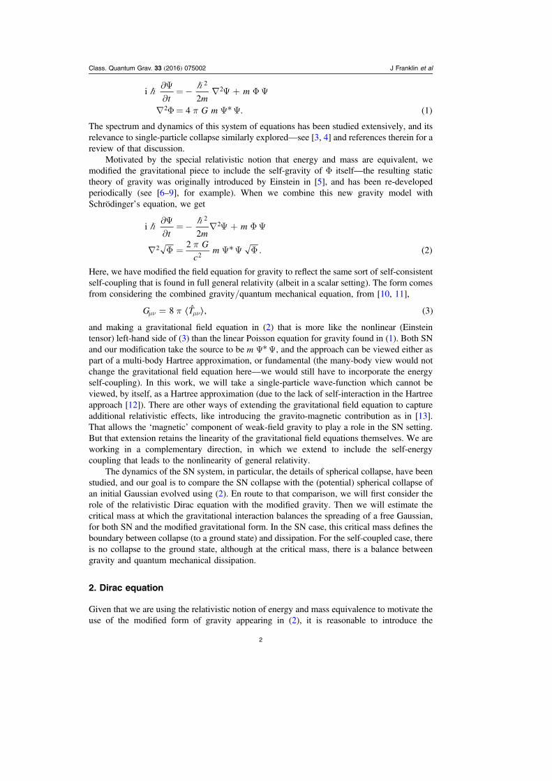
Figure 1. The (dimensionless) energy, as a function of mass (in units of Planck mass),for the ground state of the modified-gravity-Dirac system is shown with black dots. Thesame calculation using a Newtonian gravitational field and the Dirac equation is shownin gray dots, and the solid line is the SN ground state energy, for comparison.

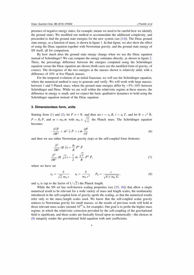
Figure 2. The percentage difference between the ground state energies as computedusing the Dirac equation and the Schrödinger equation. Mass is in units of Planck mass.

Class. Quantum Grav. 33 (2016) 075002 J Franklin et al

3

presence of negative energy states, for example, means we need to be careful how we identifythe ground state). We modified our method to accommodate the additional complexity, andproceeded to find the ground state energies for the new system (see [14]). The Dirac groundstate energy, as a function of mass, is shown in figure 1. In that figure, we also show the effectof using the Dirac equation together with Newtonian gravity, and the ground state energy ofSN itself, all for comparison.

By how much does the ground state energy change when we use the Dirac equationinstead of Schrödinger? We can compare the energy estimates directly, as shown in figure 2.There, the percentage difference between the energies computed using the Schrödingerequation versus the Dirac equation are shown (both cases use the modified form of gravity, ofcourse). The divergence of the two energies at the masses shown is relatively mild, with adifference of 10% at five Planck masses.

For the temporal evolution of an initial Gaussian, we will use the Schrödinger equation,where the numerical method is easy to generate and verify. We will work with large masses,between 1 and 5 Planck mass, where the ground state energies differ by ∼5%–10% betweenSchrödinger and Dirac. While we are well within the relativistic regime at these masses, thedifference in energy is small, and we expect the basic qualitative dynamics to hold using theSchrödinger equation instead of the Dirac equation.

3. Dimensionless form, units

Starting from (1) and (2), let P rw :, and then set r r R0� , t t T0� , and let c2 ¯' � ',

P P P0 ¯� , and m m m0 ¯� with m cG0�w the Planck mass. The Schrödinger equation

becomes

PR

m P mPT

i 62

22

¯¯ ¯ ¯ ¯

¯( )G�

ss

� �ss

and then we use either Newtonian gravity (top) or the self-coupled form (bottom):

RR

mR

P P

RR m

RP P

12

, 7

2

2

2

2

( ¯ ) ¯ ¯ ¯

( ¯ ) ¯¯ ¯ ¯ ( )

*

*

G

GG

ss

�

ss

�

where we have set

rm c

tm c

Pc

m G2 4, 80

00

02 0

0( )� �

Q� � �

and r0 is (up to the factor of 1 2 ) the Planck length.While the SN set has well-known scaling properties (see [15, 16]) that allow a single

numerical result to be relevant for a wide variety of mass and length scales, the nonlinearityintroduced in the self-coupled form of gravity spoils the scaling, so that the numerical resultsrefer only to the mass/length scales used. We know that the self-coupled scalar gravityreduces to Newtonian gravity for small masses, so the results of previous work will hold atthose relevant mass scales (around 1010 u, for example). Our goal is to probe the higher massregime, in which the relativistic correction provided by the self-coupling of the gravitationalfield is significant, and these scales are basically forced upon us numerically—the choices in(8) uniquely render the gravitational field equation with unit coefficients.

Class. Quantum Grav. 33 (2016) 075002 J Franklin et al

4

We will start with a spherically symmetric Gaussian wave function:

r a, 0 e , 9r a2 3 4 22 2( ) ( ) ( )( )Q: � � �

where a2 is the variance (up to constants) of the initial distribution. Then our initial,dimensionless P is

P R r R r R P A R, 0 , 0 22

e 10R A0 0 0

1 43 2 22 2¯ ( ) ( ) ( )( )⎜ ⎟⎛

⎝⎞⎠Q

� : � � �

with a r A0� . The normalization of the wave function, in the dimensionless setting, is

P P RP r

d1

42 . 11

0 02

0

¯ ¯ ( )*¨ Q� �

d

For our initial Gaussians, we will take a r0� , so that A=1. While we can make Alarger to spread out the initial distribution of mass as a source for gravity, there is no naturalmultiple of r0 to use—one might try to extend the distribution beyond, for example, itsSchwarzschild radius (at m2 2 ¯ in these dimensionless units)— but then the mass requiredto achieve collapse also increases, and the initial distribution ends up inside the Schwarzschildradius again3. In order to compare with potential experiments, the relevant scale isa 0.5 10 6� q � m (as in [17]), but in our units, this leads to A 4 1028_ q , inappropriatelylarge for numerical work. At the low densities implied by taking a 0.5 mN� , we know thatthe predictions of the self-coupled form of gravity match the Newtonian case. ChoosingA=1 allows us to probe the regime in which Newtonian gravity must be augmented by theself-gravity of the field (and additional, as yet unknown, physics).

4. Numerical method

The collapse dynamics of SN have been studied in [16–19], and all use similar methods totime-evolve initial Gaussians: some variant of Crank–Nicolson and a solver for the gravita-tional Poisson problem in iterative combination. Our method is similar, when applied to SN,although we use Verlet to find the gravitational field (as opposed to quadrature or a pseudo-spectral method). Verlet is easy to apply to the nonlinearity present in the self-coupledgravitational field equation, with its more complicated boundary conditions. The pieces(Crank–Nicolson and Verlet) can be described separately, but then an iterative step must beinvolved to achieve a self-consistent solution. We start by discretizing in space and time viaR j Rj � % and T n Tn � % for constant spacings R% , T% . We will call the value of P (atlocation Rj and time Tn) P R T P,j n j

n¯ ( ) ¯w , and similarly R T,j n jn¯ ( ) ¯G Gw .

The forward-Euler discretization in time, for the Schrödinger piece, reads

P Pm

TP P P

Rm P

i 2. 12j

njn j

njn

jn

jn

jn1 1 1

22¯ ¯

¯¯ ¯ ¯

¯ ¯ ¯ ( )⎡⎣⎢⎢

⎤⎦⎥⎥G� � % �

� �

%�� � �

This equation holds for all grid points, and we understand that at j=0, we have P 0n0

¯ � forall n, that’s the boundary condition at the origin (for Ψ finite at the origin, as it should be,P r� : will be zero at the origin). The spatial grid will extend to R N R� %d for integer N,our choice of numerical infinity, and out there we will again set P 0;N

n1

¯ �� the wave functionshould vanish.

3 The Schwarzschild radius is, of course, external to either the Newtonian or self-coupled gravities considered here—it represents an artificial length, from the point of view of the current work, and we understand that to trulydescribe the physics at this scale, additional gravitational elements (at the very least) are necessary.

Class. Quantum Grav. 33 (2016) 075002 J Franklin et al

5

Let the vector Pn¯ contain the (unknown) spatial values at time level n:

PP

P

P . 13n

n

n

Nn

1

2¯ ˙ ( )

⎛

⎝

⎜⎜⎜⎜

⎞

⎠

⎟⎟⎟⎟�

#

and similarly for the vector nG . Then we can write the forward Euler discretization (togetherwith the boundary conditions) in terms of a matrix-vector multiplication:

P PTi 14n n n1¯ ( ( ¯ )) ¯ ( )� � G� � %�

where � is the identity matrix, n( ¯ )� G is defined by (12), and we highlight its dependence onthe gravitational potential.

The backwards Euler version of the problem is

T P Pi , 15n n n1 1( ( ¯ )) ¯ ¯ ( )� � G� % �� �

and then the Crank–Nicolson method is defined by

T TP Pi

2i

2. 16n n n n1 1( ¯ ) ¯ ( ¯ ) ¯ ( )⎛

⎝⎜⎞⎠⎟

⎛⎝⎜

⎞⎠⎟� � � �G G�

%� �

%� �

For the gravitational field portion, we will use Verlet, although the details will changeslightly between the two forms of gravity for reasons that will become clear as we go. ForNewtonian gravity, we start at ‘spatial infinity’ (out at RN) with the Newtonian limiting form:

R1 2Nn

NG � � and R1 2Nn

N1 1G � �� � —the constant term provides a constant offset(c2 when units are introduced) that doesn’t effect the probability density here, but weintroduce it for comparison with the modified gravity. Starting at N, we move inwardsaccording to the Verlet update:

RR R R

mR

P1

2 . 17jn

jjn

j jn

jj

jn

11

1

111

12 1 2¯ ¯ ¯ ¯ ∣ ∣ ( )

⎛⎝⎜⎜

⎛⎝⎜

⎞⎠⎟

⎞⎠⎟⎟G G G� � � %�

�

�

���

��

The procedure for modified gravity is a little different—at spatial infinity, we know thatNewtonian gravity, for a spherically symmetric source of mass m, must limit to G m

r� (or

c G mr

2 � if a constant offset is desired). But for the modified gravitational field, we have

c G mr

2 ˜� as the leading contribution at spatial infinity—the c2 is required so that the modifiedsolutions become Newtonian in the non-relativistic limit (see [9]), and the ‘mass’ m dependson the details of the central distribution (for example, a point mass m at the origin and asphere of homogeneous mass density and total mass m, lead to different values for m). Sincethe central distribution of mass will change here, the value for m is a function of time, acomplication we’d like to avoid.

Instead, we will focus on the value of the field as r 0l . For a sphere with homogenousmass density, the internal field r( )' looks like (see [8, 9])

cR r

r rr rcosh

sinh, 18

0

0

0

2

( )( ) ( )

⎡⎣⎢

⎤⎦⎥' �

where R is the radius of the sphere and r0 is a constant related to the mass. As r 0l , f goesto a constant bounded by c2, and the derivative of f goes to zero. Since we expect there to besome non-zero density near the origin, these are reasonable boundary conditions for ournumerical solution, i.e. Cn

0G � a constant 0, 1[ ]� and Cn1G � , so that the numerical

Class. Quantum Grav. 33 (2016) 075002 J Franklin et al

6

derivative is approximately zero. We will pick C so that 1NnG � , its limiting value, at spatial

infinity (the best we can do here) by shooting—i.e. we will run forward Verlet:

RR R R

mR

P1

22

. 19jn

jjn

j jn

jj

jn

jn

11

1

111

12 1 2 1¯ ¯ ¯ ¯ ∣ ∣ ¯ ( )

⎡⎣⎢⎢

⎛⎝⎜

⎞⎠⎟

⎤⎦⎥⎥G G G G� � � %�

�

�

���

�� �

for different values of C n n0

11

1G G� �� � until 1NnG x , using bisection to determine C

accurately.In both of these cases, Newtonian and modified, we must iterate at each time level to

achieve a self-consistent solution—notice that the left-hand side of (16) depends on n 1G � ,which we can only get once Pn 1¯ � is known—but we cannot findPn 1¯ � without n 1G � . To breakout of the recursion, we will define an iterative index k –let Pk n 1¯ � and k n 1G � be the kiteration at time-level n 1� . For k=0, we define P Pn n0 1¯ ¯�� and n n0 1¯ ¯G G�� . Now, atlevel k, we update (using the Newtonian update for simplicity) according to:

T T

RR R R

mR

P

P Pi2

i2

12 , 20

k n k n n n

kjn

j

kjn

jk

jn

jj

kjn

1 1 1

111

1

1 1 111

12 1 1 2

( ¯ ) ¯ ( ¯ ) ¯

¯ ¯ ¯ ¯ ∣ ∣ ( )

⎛⎝⎜

⎞⎠⎟

⎛⎝⎜

⎞⎠⎟

⎛⎝⎜⎜

⎛⎝⎜

⎞⎠⎟

⎞⎠⎟⎟

� � � �G G

G G G

�%

� �%

� � � %

� � �

���

�

� � ���

�� �

where the top line defines the new value for the wave function, and the second line updatesthe gravitational field. We proceed with this iteration until

P P , 21k n k n1 1 1¯ ¯ ( )�� �� � �& &

where � is given—i.e. we continue to iterate until the wave function has stopped changingsignificantly. Once we have achieved (numerical) convergence, we set P Pn k n1 1 1¯ ¯�� � � and

n k n1 1 1¯ ¯G G�� � � , and we’re ready to move on to the next time step.

5. Critical mass estimate

The goal of this section is to establish mass values for which the behavior of the initialGaussian shifts from ‘mainly quantum’, with the initial Gaussian spreading out over time, to‘mainly gravitational’, with the initial Gaussian becoming more localized. One simple way toestimate this mass, from [16], is to take the free particle solution for the initial Gaussian,which is:

r t at

m a, 1

ie 222 3 4

2

3 2 r

a tm a

2

2 2 1 i2( ) ( ) ( )⎜ ⎟⎛

⎝⎞⎠

⎛⎝⎜

⎞⎠⎟� �

Q: � ��� �

�

and note that the peak of r r t r t, ,2 ( ) ( )*: : is located at

r t at

am. 23p

22

( ) ( )⎜ ⎟⎛⎝

⎞⎠

�� �

With no gravitational component, r 0p a m

2

3 2( ) �� , the initial acceleration of the most-likelyposition depends only on m (and the initial variance). With a gravitational force in place, wehave:

Class. Quantum Grav. 33 (2016) 075002 J Franklin et al

7

rr

r a¨ 0dd

0 0 , 24p p net( ) ( ( )) ( ) ( )⎜ ⎟⎛⎝

⎞⎠� � ' �

where a 0net ( ) is the net acceleration (treating the most-likely position as the particle position),and we could arrange to have a 0 0net ( ) � by taking:

rr

r¨ 0dd

0 . 25p p( ) ( ( )) ( )� '

The r( )' that we use depends on both our choice to consider Newtonian or self-coupledgravity, and the ρ that we decide to use to approximate the initial distribution of ‘mass’ (in[16], for example, a point particle at the origin is used to perform this estimate4. Since wehave a Gaussian profile, we can take m *S � : : for the initial Ψ given in (9) and use that tosolve for r( )' . For Newtonian gravity, the field associated with this source is

rGm

rra

erf , 26( ) ( )⎜ ⎟⎛⎝

⎞⎠' � �

and using this in (25) with r=a (the initial value) gives

ha m

Gma e

Gma

2erfc 1 . 27

2

3 2 2 2( ) ( )

Q� �

Since we’ve taken a r0� , we have aGm2

2

03

�� (in terms of the Planck mass m0), and we can

get rid of ÿ using the Planck mass definition, ;G mc

02

� � then the solution to this equation is

m m m2

1 erfc 11.5 . 28

e

1 6

2 0 0( )( )�

� �x

Q

For the modified form of gravity, we cannot find r( )' explicitly, so we turn to anumerical approach. Given the numerical parameters we will use below, we compute the 'from the initial source (the dimensionless m P P¯ ¯ ¯* with P and A=1 from (10), projected ontoour numerical grid) using the Verlet method described in section 4, then approximate thederivative using finite difference (suitably dimensionless, which throws in a factor of 2) andevaluate that at r 1¯ � (a in our dimensionless units), we subtract

m4

2¯ (the dimensionless formof r 0p ( ) here) and then find m such that the difference is close to zero (to within 10 5� � � ). Aplot of the difference:

Figure 3. The dimensionless numerical acceleration, z, from (29), as function of m.

4 While this simplified estimate works well for Newtonian gravity, using the point source solution for the modified,self-coupled gravity would yield no real m that satisfied (25), so we must use a more realistic distribution.

Class. Quantum Grav. 33 (2016) 075002 J Franklin et al

8

zm R4

22

29p p2

1 1

¯¯ ¯

( )G G

w ��

%� �

with p R 1% x is shown in figure 3, where we can see that the root lies in between m 3¯ �and 4. A bisection of z gives m 3.3¯ x as the mass associated with the onset of contractingbehavior.

6. Numerical dynamics

The numerical results agree well with the predictions from above. In all cases, we takeN=1000 spatial steps, with R 50�d , and set T 0.1% � . We can plot the probabilitydensities as functions of time, for the n=1, 50 and 100 steps to see what sort of evolution ishappening. Following [16], we also plot the radius in which 90% of the probability lies, this‘R T90 ( )’ value allows us to track the general evolution in time. We will plot that together withthe value associated with a free Gaussian, so we can see what effect gravity (in its variousforms) has. We can further characterize the dynamics by calculating the overlap of the wavefunction with the ground state (calculated using the methods of [2]) as a function of time.

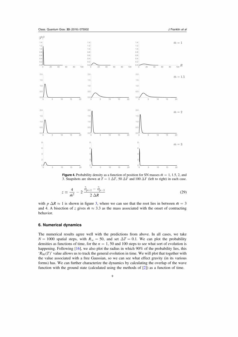
Figure 4. Probability density as a function of position for SN masses m 1¯ � , 1.5, 2, and3. Snapshots are shown at T T1� % , T50 % and T100 % (left to right) in each case.

Class. Quantum Grav. 33 (2016) 075002 J Franklin et al

9

The Crank–Nicolson method we use here is not obviously norm-preserving, unlike theoriginal one. That lack of manifest norm preservation comes from the time-dependence of thematrix operator � appearing on the left and right sides of (16). Yet in practice, the norm ispreserved well in all the runs, with the maximum difference between the numerical norm and

2 (the appropriate normalization from (11)) on the order of 10−13.For SN, the probabilities are shown in figure 4 for m 1¯ � , 1.5, 2 and 3, and a plot of

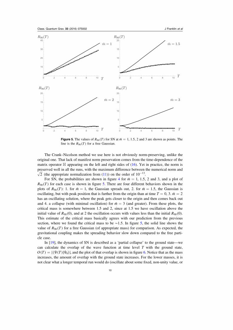
R T90 ( ) for each case is shown in figure 5. There are four different behaviors shown in theplots of R T90 ( ): 1. for m 1¯ � , the Gaussian spreads out, 2. for m 1.5¯ � , the Gaussian isoscillating, but with peak position that is further from the origin than at time T=0, 3. m 2¯ �has an oscillating solution, where the peak gets closer to the origin and then comes back outand 4. a collapse (with minimal oscillation) for m 3¯ � (and greater). From these plots, thecritical mass is somewhere between 1.5 and 2, since at 1.5 we have oscillation above theinitial value of R 090 ( ), and at 2 the oscillation occurs with values less than the initial R 090 ( ).This estimate of the critical mass basically agrees with our prediction from the previoussection, where we found the critical mass to be ∼1.5. In figure 5, the solid line shows thevalue of R T90 ( ) for a free Gaussian (of appropriate mass) for comparison. As expected, thegravitational coupling makes the spreading behavior slow down compared to the free parti-cle case.

In [19], the dynamics of SN is described as a ‘partial collapse’ to the ground state—wecan calculate the overlap of the wave function at time level T with the ground state,O T T 0( ) ∣⟨ ( )∣ ⟩∣� : : , and the plot of that overlap is shown in figure 6. Notice that as the massincreases, the amount of overlap with the ground state increases. For the lower masses, it isnot clear what a longer temporal run would do (oscillate about some fixed, non-unity value, or

Figure 5. The values of R T90 ( ) for SN at m 1¯ � , 1.5, 2 and 3 are shown as points. Theline is the R T90 ( ) for a free Gaussian.

Class. Quantum Grav. 33 (2016) 075002 J Franklin et al

10

increase towards full overlap), but for m 2¯ � and 3, a clear trend towards collapse to theground state is shown.

Making the same plots for the self-coupled gravity case (with densities in figure 7 andR T90 ( ) shown in figure 8), at masses m 2¯ � , m 3¯ � , m 4¯ � and m 10¯ � , we again see thespreading behavior at m 2¯ � , and at m 3¯ � , oscillation has begun. This oscillation does notrepresent collapse, though, as can be seen in figure 8, the oscillation occurs at values abovethe initial R 090 ( )—there is no contraction here. It is not until m 4¯ � that oscillation withvalues below the initial R 090 ( ) occurs. So we would put the critical mass somewhere betweenm 3¯ � and 4, again agreeing with our estimate ∼3.3. What is surprising in this case is the lackof decay we saw in, for example, m 3¯ � of SN (both in the plot of R T90 ( ) and in O(T)).Instead, in the self-coupled case, all masses display oscillatory behavior without ‘settlingdown’ (we have run up to masses of m 20¯ � , but still see no sign of a collapse to the groundstate).

This lack of convergence can also be seen in the plots of the overlap with the ground state(calculated, appropriately, for the self-coupled case), shown in figure 9. Instead of oscillatingtowards an overlap of1 with the ground state, as in SN, the overlap in the self coupled case doesnot increase (on average) over time (for the time scales considered here). As another contrastingfeature—in figure 6, the amount of (time-averaged) overlap increases with mass, while infigure 9, the magnitude of the overlap increases, but then decreases as mass gets larger.

7. Conclusion

The inclusion of the self-coupling for gravity changes the spherical dynamics at large masses;while the expected qualitative behavior, free spreading and oscillation, occur in the expanded

Figure 6. The overlap of the wave function at time T with the ground state (atappropriate mass) for SN.

Class. Quantum Grav. 33 (2016) 075002 J Franklin et al

11

gravitational setting, the mass scales at which they occur are roughly twice those of New-tonian gravity. We estimated the mass scales using a simple equivalence of quantummechanical ‘acceleration’ and the gravitational field associated with our initial Gaussian wavefunction, and that estimate agreed fairly well with the numerical solutions. The collapse to theground state, apparent for SN at masses above m 2¯ � here, is absent from the self-coupledcase (at the time scales considered here—time scales which are relevant for the SN case, atleast).

Because we are using a form of gravity inspired by special relativistic mass–energyequivalence, we first calculated the energy spectrum of the quantum-mechanical/self-coupledgravitational system using the Dirac equation, to compare with the previously publishedSchrödinger spectrum, and found that, for the masses of interest to us at collapse, the error inthe ground state energy is 10%_ , this suggests we can use the Schrödinger equation to evolvethe initial Gaussian forward in time without incurring too much error. For comparison, thedifference between the ground state energy for SN and Dirac with self-coupled gravityis 600%_ .

Figure 7. Probability density as a function of position for self-coupled gravity massesm � 2, 3, 4 and 10. Snapshots are shown at T = 1ΔT, 50ΔT and 100ΔT (left to right)in each case. (Note the change in vertical scale).

Class. Quantum Grav. 33 (2016) 075002 J Franklin et al

12

Figure 8. The values of R T90 ( ) for the self-coupled form of gravity at m 2, 3, 4¯ � and10 are shown as points. The line is the R T90 ( ) for a free Gaussian.

Figure 9. The overlap of the wave function at time T with the ground state (atappropriate mass) for the self-coupled case.

Class. Quantum Grav. 33 (2016) 075002 J Franklin et al

13

Self-coupled gravity does not appear to collapse to its ground state (or any other); thewave function does not achieve a relatively static steady state, as it does in SN, nor does it‘converge’ (in overlap) to its ground state. It would be interesting to establish, analytically,that the ground state in the self-coupled form of gravity is dynamically unstable, leading tothe observed oscillation without the decay to the ground state present in SN. Another potentialissue is our use of the Schrödinger equation—perhaps at higher mass values, where the Diracequation is relevant, we would find a damped-oscillatory collapse for the self-coupled gravity.

References

[1] Ruffini R and Bonazzola S 1969 Phys. Rev. 187 1767–83[2] Franklin J, Guo Y, McNutt A and Morgan A 2015 Class. Quantum Grav. 32 065010[3] Carlip S 2008 Class. Quantum Grav. 25 154010

Salzman P J and Carlip S 2006 arXiv:gr-qc/0606120[4] Giulini Domenico and Großart André 2012 Class. Quantum Grav. 29 215010[5] Einstein A 1912 Zur Theorie des statschen gravitationsfeldes Ann. Phys. (Leipzig) 38 443–58

Einstein A 1996 The Collected Papers of Albert Einstein vol 4 (Princeton, NJ: PrincetonUniversity Press) pp 107–120 (Engl. transl. by Anna Beck)

[6] Deser S and Halpern L 1970 Gen. Relativ. Gravit. 1 131–6[7] Freund P G O and Nambu Y 1968 Phys. Rev. 174 1741–3[8] Giulini D 1997 Phys. Lett. A 232 165–70[9] Franklin J 2015 Am. J. Phys. 83 332–7[10] Møller Les C 1962 Les Théories Relativistes de la Gravitation (Colloques Internationaux CNRS

vol 91) ed A Lichnerowicz and M-A Tonnelat (Paris: CNRS)[11] Rosenfeld L 1963 Nucl. Phys. 40 353[12] Adler S L 2007 J. Phys. A: Math. Theor 40 755–64[13] Manfredi G 2015 Gen. Relativ. Gravit. 47 1–12[14] Guo Y 2015 Scalar gravity with self-eld coupling PhD thesis Reed College, Portland, OR[15] Moroz I M, Penrose R and Tod P 1998 Class. Quantum Grav. 15 2733–42[16] Giulini D and Großart A 2011 Class. Quantum Grav. 28 195026[17] Salzman P J 2005 Investigation of the time dependent Schrödinger–Newton equation Dissertation

University of California DavisSalzman P J and Carlip S 2006 arXiv:gr-qc/0606120

[18] Harrison R, Moroz I and Tod K P 2003 Nonlinearity 16 101–22Harrison R 2001 A numerical study of the Schrödinger–Newton equations Dissertation University

of Oxford[19] van Meter J R 2011 Class. Quantum Grav. 28 215013

Class. Quantum Grav. 33 (2016) 075002 J Franklin et al

14