Embed Size (px)
Citation preview
The Dynamics of High-Frequency
Nanoelectromechanical
Resonators in Fluid
Douglas Richard Brumley
Thesis submitted in partial requirement of the degree
of
Bachelor of Science (Honours)
November 2008
The University of Melbourne
Department of Mathematics and Statistics
Supervisor: Prof. John E. Sader


Abstract
When a silicon carbide beam clamped at both ends is excited thermoelastically, it ex-
hibits a spectrum of in-plane and out-of-plane resonances. We present several original
formulations to determine the quality factors associated with the in-plane modes when
the beam is immersed in a gas. We analyse several different fluid-beam boundary con-
ditions, and account for the effects of slip. The model predictions agree quantitatively
with the experimental values obtained by the Roukes group from California Institute
of Technology.

Contents
1 Introduction 1
2 Nanoelectromechanical Systems (NEMS) 5
2.1 Assumptions . . . . . . . . . . . . . . . . . . . . . . . . . . . . . . . . . 8
2.2 Boundary Conditions . . . . . . . . . . . . . . . . . . . . . . . . . . . . . 9
2.3 Hydrodynamic Function . . . . . . . . . . . . . . . . . . . . . . . . . . . 11
2.4 Quality Factors . . . . . . . . . . . . . . . . . . . . . . . . . . . . . . . . 12
2.5 Experimental Results . . . . . . . . . . . . . . . . . . . . . . . . . . . . . 13
3 Resonant Frequencies in Vacuum 15
3.1 Free Vibrations . . . . . . . . . . . . . . . . . . . . . . . . . . . . . . . . 15
3.2 Free Vibrations - Intrinsic Tension . . . . . . . . . . . . . . . . . . . . . 18
3.2.1 Euler Buckling Formula . . . . . . . . . . . . . . . . . . . . . . . 23
4 High-Frequency Limit 25
4.1 No-Slip Boundary Condition . . . . . . . . . . . . . . . . . . . . . . . . 26
4.2 Second-Order Slip Boundary Condition . . . . . . . . . . . . . . . . . . 27
4.3 Matched Asymptotic Expansion . . . . . . . . . . . . . . . . . . . . . . . 29
4.4 Progressive Comparison With Experiment . . . . . . . . . . . . . . . . . 33
5 Beam of Zero Thickness 35
5.1 No-Slip Boundary Condition . . . . . . . . . . . . . . . . . . . . . . . . 38
5.1.1 Numerical Solution Method . . . . . . . . . . . . . . . . . . . . . 40
5.1.2 Calculation of Hydrodynamic Function . . . . . . . . . . . . . . . 43
5.2 Second-Order Slip Boundary Condition . . . . . . . . . . . . . . . . . . 46
5.2.1 Numerical Solution Method . . . . . . . . . . . . . . . . . . . . . 48
i

5.2.2 Calculation of Hydrodynamic Function . . . . . . . . . . . . . . . 51
5.3 Alternative Solution Method for First-Order Slip . . . . . . . . . . . . . 53
5.4 High-Frequency Limit . . . . . . . . . . . . . . . . . . . . . . . . . . . . 55
5.5 Convergence With Mesh Discretization . . . . . . . . . . . . . . . . . . . 58
5.6 Progressive Comparison With Experiment . . . . . . . . . . . . . . . . . 61
6 Beam of Non-Zero Thickness 63
6.1 No-Slip Boundary Condition . . . . . . . . . . . . . . . . . . . . . . . . 64
6.1.1 Numerical Solution Method . . . . . . . . . . . . . . . . . . . . . 70
6.1.2 Calculation of Hydrodynamic Function . . . . . . . . . . . . . . . 76
6.1.3 Alternative Scaling For Out-of-Plane Modes . . . . . . . . . . . . 79
6.2 First-Order Slip Boundary Condition . . . . . . . . . . . . . . . . . . . . 82
6.2.1 Numerical Solution Method . . . . . . . . . . . . . . . . . . . . . 87
6.2.2 Calculation of Hydrodynamic Function . . . . . . . . . . . . . . . 91
6.2.3 Comparison with Free Molecular Solution . . . . . . . . . . . . . 96
6.3 Progressive Comparison With Experiment . . . . . . . . . . . . . . . . . 98
6.4 Determination of Surface Properties . . . . . . . . . . . . . . . . . . . . 99
7 Concluding Remarks 103
A Richardson Extrapolation 105
B Matched Asymptotic Solutions 107
B.1 Beam of Zero Thickness . . . . . . . . . . . . . . . . . . . . . . . . . . . 107
B.2 Beam of Non-Zero Thickness . . . . . . . . . . . . . . . . . . . . . . . . 112
ii

List of Figures
1.1 Scanning electron micrograph of device . . . . . . . . . . . . . . . . . . . 2
1.2 Schematic diagram of clamped-clamped beam . . . . . . . . . . . . . . . 3
3.1 Predicted resonant frequencies . . . . . . . . . . . . . . . . . . . . . . . 21
4.1 Asymptotic solutions for infinite plate . . . . . . . . . . . . . . . . . . . 32
4.2 Predicted quality factors: high-frequency limit . . . . . . . . . . . . . . 34
5.1 Cross-section of beam of zero thickness . . . . . . . . . . . . . . . . . . . 35
5.2 Vorticity distribution for beam of zero thickness: no-slip condition . . . 43
5.3 Vorticity distribution for beam of zero thickness: no-slip condition . . . 49
5.4 Vorticity distribution for beam of zero thickness: first-order slip condition 50
5.5 Vorticity distribution for beam of zero thickness: second-order slip con-
dition . . . . . . . . . . . . . . . . . . . . . . . . . . . . . . . . . . . . . 51
5.6 Hydrodynamic function for beam of zero thickness . . . . . . . . . . . . 52
5.7 Convergence of hydrodynamic function with β . . . . . . . . . . . . . . 56
5.8 Convergence of hydrodynamic function with N . . . . . . . . . . . . . . 58
5.9 Beam of zero thickness: perturbation solutions . . . . . . . . . . . . . . 60
5.10 Predicted quality factors: beam of zero thickness . . . . . . . . . . . . . 62
6.1 Cross-section of beam of non-zero thickness . . . . . . . . . . . . . . . . 63
6.2 Integration contour enclosing entire fluid . . . . . . . . . . . . . . . . . . 66
6.3 Integration contour around beam of non-zero thickness . . . . . . . . . . 68
6.4 Vorticity and pressure distribution on front face of beam: no-slip . . . . 74
6.5 Vorticity and pressure distribution on top face of beam: no-slip . . . . . 75
6.6 Hydrodynamic function for beam of non-zero thickness . . . . . . . . . . 78
iii

6.7 Convergence of hydrodynamic function with aspect ratio A . . . . . . . 80
6.8 Vorticity and pressure distribution on front face of beam: first-order slip 89
6.9 Vorticity and pressure distribution on top face of beam: first-order slip . 90
6.10 Behaviour of hydrodynamic function with Knudsen number . . . . . . . 91
6.11 Linear components of hydrodynamic function . . . . . . . . . . . . . . . 93
6.12 Hydrodynamic function as a Pade approximant . . . . . . . . . . . . . . 94
6.13 Convergence of hydrodynamic function with N . . . . . . . . . . . . . . 95
6.14 Comparison between computed hydrodynamic function and free molec-
ular solution . . . . . . . . . . . . . . . . . . . . . . . . . . . . . . . . . . 97
6.15 Predicted quality factors: beam of non-zero thickness . . . . . . . . . . . 100
B.1 Asymptotic solutions for infinitely thin blade of finite width . . . . . . . 110
B.2 Three distinct flow regimes around blade . . . . . . . . . . . . . . . . . . 111
iv

List of Tables
2.1 Experimental quality factors . . . . . . . . . . . . . . . . . . . . . . . . . 13
3.1 Resonant frequencies for beam of length 8µm . . . . . . . . . . . . . . . 18
3.2 Resonant frequencies for beam of length 16µm . . . . . . . . . . . . . . 18
4.1 Quality factors: high-frequency limit . . . . . . . . . . . . . . . . . . . . 33
5.1 Quality factors: beam of zero thickness . . . . . . . . . . . . . . . . . . . 61
6.1 Quality factors: beam of non-zero thickness (unfitted) . . . . . . . . . . 98
6.2 Quality factors: beam of non-zero thickness (fitted) . . . . . . . . . . . . 100
v

“The choice is always the same. You can make your model more complex and more
faithful to reality, or you can make it simpler and easier to handle. Only the most
naive scientist believes that the perfect model is the one that perfectly represents reality.
Such a model would have the same drawbacks as a map as large and detailed as the city
it represents, a map depicting every park, every street, every building, every tree, every
pothole, every inhabitant, and every map. Were such a map possible, its specificity
would defeat its purpose: to generalize and abstract. Mapmakers highlight such features
as their clients choose. Whatever their purpose, maps and models must simplify as
much as they mimic the world.” – James Gleick
vi


Acknowledgements
I would sincerely like to thank John Sader for the many exciting discussions. The
support and encouragement I have received has been phenomenal.
Thanks must also go to Igor Bargatin and the Roukes Group from California Institute
of Technology for their amazing experimental work.
I am indebted to my wonderful family and friends – in particular Naomi Clarke,
Harrison Wraight and Jason Nassios – for their patience and understanding over the
past year.
viii

ix

Chapter 1
Introduction
Nanoelectromechanical systems (NEMS) enable exquisitely sensitive measurements
to be taken at the nano-scale. The dynamics of fluid systems at this level can be vastly
different to those of the macroscopic world with which we are most familiar. Much re-
search has been undertaken in an attempt to gain an appreciation of how nano-devices
function, as well as the principles governing fluid motion, at this scale. The practical
applications are very exciting indeed. For example, an understanding of the dynamics
of thin cantilever beams has led to the widespread use of the atomic force microscope,
capable of identifying individuals atoms. Furthermore, the extreme sensitivity of other
NEMS devices has facilitated zeptogram-scale (10−21g) mass sensing [1] .
A comprehensive knowledge of the underlying physical principles is essential in
harnessing the enormous potential that NEMS devices offer. In this thesis, we explore
the dynamics of one such device. When a clamped-clamped silicon carbide beam is
excited thermoelastically, it exhibits a spectrum of in-plane and out-of-plane resonances.
Recent experiments conducted by Bargatin et al. [2] involved immersing such beams
in a gas and measuring the quality factors associated with the exhibited resonances.
The quality factor Q is a dimensionless parameter that relates the stored energy in the
beam to the rate of energy dissipation. The beams used by Bargatin et al. [2] have
a width of 400nm, a thickness of 80nm and vary in length between 8µm and 24µm.
Consider Fig. 1.1, which shows a scanning electron micrograph of one such device.
Motion of the beam is initiated electrically through thermal expansion. The electrical
resistance of components of the beam depend on the mechanical stresses present and
1

2
thus the deflection. This allows for the motion to be detected and processed using a
metal piezoresistor.
Figure 1.1: Scanning electron micrograph of one of the devices used by Bargatin et al. [2](oblique view). The top two insets are close-up images showing the drive (right) and detection(left) loops.
Consider the illustrations in Fig. 1.2 which clearly show both the nature of the
apparatus and the motions it can execute. We emphasise that the in-plane and out-of-
plane movements depicted are the fundamental modes only. The beams exhibit many
mode shapes in the experiments [2].
As the beam vibrates, it loses energy due to both internal dissipation and damp-
ing by the surrounding fluid. The rate at which energy is lost from the beam can be
measured, and is found to exhibit a strong dependence on the frequency of oscillation.
The problem with which we are faced is to develop an understanding of the energy
dissipation in these systems.
We will begin by analysing the beam as a linearly elastic body and predict the
resonant frequencies in vacuum. In Chapter 4 we assess the dynamics of the beam in a
viscous fluid, operating in the high-frequency limit. Chapters 5 and 6 account for the
finite dimensions of the beam, and successfully incorporate the effects of slip. These
final two chapters constitute original research and provide a significant contribution
towards the understanding of NEMS devices. At the end of each chapter we will assess
the accuracy of the model by comparing the predictions with experimental results.

Chapter 1. Introduction 3
h
b
L
x
y
z
(a)
(b) (c)
Figure 1.2: (a) Diagram of clamped-clamped beam. The origin of the coordinate systemis located at the geometric centre of the cross-section of the beam at the left clamped end(depicted by a small black dot). (b) Schematic diagram showing out-of-plane motion. (c)Schematic diagram showing in-plane motion.


Chapter 2
Nanoelectromechanical Systems
(NEMS)
Micro-cantilever beams have been used in atomic force microscopy (AFM) for a
number of years. Significant work — both experimental and theoretical — has been un-
dertaken in an attempt to understand the behavior of such elastic devices. Knowledge
of the frequency spectra is paramount in application to the atomic force microscope
[3]. The frequency response of an elastic beam is highly sensitive to the nature of the
fluid in which it is immersed. In order to accurately predict the frequency spectrum,
we must take into account the physical properties of the beam, as well as the nature of
the surrounding fluid.
In 1851 Stokes [4] provided an analytical solution to the problem involving a cylin-
der of circular cross-section oscillating in a viscous fluid. He found that during such
oscillations, the cylinder experienced viscous losses due to the surrounding fluid, as well
as an added (or “virtual”) mass component. In 1969, Tuck [5] presented a boundary in-
tegral formulation whereby the hydrodynamic loading could, in principle, be calculated
for a cylinder of arbitrary cross-section. Whilst Tuck’s solution was quite general, the
absence of powerful computers limited the circumstances to which it could be applied.
We will use this boundary integral technique extensively throughout the course of our
problem. It must be noted that the assumptions made by Tuck in deriving his result
are also adopted in our problem formulation.
5

6
Since the publication of Tuck’s paper in 1969, much work has been done in de-
termining the frequency response of cantilevers subject to a driving force. The driving
force is often due to thermal oscillations and can be modified by the presence of a nearby
surface e.g. in the case of the atomic force microscope. Typically, the surrounding fluid
is considered to be infinite in extent. However, Green [6] looked at the effects associated
with the presence of a nearby boundary in the fluid. Sader [3] analysed the frequency
response and hydrodynamic loading of both rectangular and circular cantilever beams
immersed in viscous fluids. The modes exhibited by cantilevers can be either transverse
or torsional in nature. Green and Sader [7] discussed the torsional frequency response
of rectangular cantilever beams in viscous fluids. This is of particular importance in
understanding how the atomic force microscope works.
Until recently, only out-of-plane and torsional modes have received attention. From
a practical point of view, it is relatively easy to detect and measure out-of-plane motion.
In experiments conducted by Sader et al. [8], a laser beam was used to monitor the
deflection of the cantilever. This method cannot be employed for in-plane modes since
the plane of the cantilever does not move during oscillations. In 2007, Bargatin et al. [2]
were able to detect both the in-plane and out-of-plane modes for silicon-carbide-based
beams. The devices were actuated thermoelastically at room temperature and their
motion detected piezoresistively. The piezoresistor could be used since the electrical
resistance of device-integrated metal loops depend on the mechanical stresses present.
The amplitude and frequency of oscillation could thus be calculated by analysing the
electrical signal passed through the loop.
Cantilevers of many different shapes and sizes have been studied. These include
rectangular beams, triangular and v-shaped cantilevers. The nominal width of such
devices is usually considered to greatly exceed the thickness. Consequently, the devices
studied by Green and Sader were modelled as infinitely thin.
Although cantilevers used in atomic force microscopy are typically of order 100µm
in length [8], the no-slip boundary condition traditionally used in fluid dynamics is still
applied. The mean free path of air molecules is approximately 68nm at room temper-
ature and pressure. Consequently, at small length scales, the treatment of the fluid
as a continuous medium warrants questioning. For practical applications, cantilevers

Chapter 2. Nanoelectromechanical Systems (NEMS) 7
exhibiting out-of-plane motion have been traditionally used. In such circumstances, the
effects associated with the rarefied nature of the fluid are minimal, and so treatment of
the fluid as continuous is justified.
Various slip models have, in the past been adopted in an attempt to quantify
the effects of slip. We define the Knudsen number as Kn = η/b, where η and b are
the mean free path of the fluid molecules and the dominant length scale respectively.
Hadjiconstantinou [9] outlined a second-order slip model which is claimed to extend
the applicability of Navier-Stokes solutions beyond Kn ≈ 0.1 where the accuracy of
the first-order slip model deteriorates. Hadjiconstantinou [9] presented the following
second-order boundary condition:
U∣∣wall
− uw = γη∂U
∂z
∣∣∣∣wall
− δη2 ∂2U
∂z2
∣∣∣∣wall
. (2.1)
In the above equation, γ and δ are non-adjustable parameters and η is the mean free
path of the fluid molecules. The fluid velocity field and beam velocity are denoted by U
and uw respectively. The z-direction is normal to the surface and pointing into the fluid.
For one-dimensional flows with hard spheres, we have γ = 1.11 and δ = 0.61 [9]. The
beauty of this boundary condition is that it enables the use of Navier-Stokes solutions
in a flow regime where they are usually invalid. The relative ease of determining such a
solution, compared to implementing a rigorous molecular simulation, makes this method
particularly appealing. The above values of γ and δ assume diffuse reflection of fluid
molecules from the surface. This involves the fluid molecules temporarily adhering
to the surface and subsequently being re-emitted at various velocities according to a
Maxwellian distribution [10]. If we allow for specular reflection, whereby fluid particles
simply bounce off the surface like light from a mirror, we get the following correction
for the first-order slip condition [11]:
γ →(
1.79σ
− 0.65− 0.14σ)γ.
In the above equation, 0 ≤ σ ≤ 1 is the thermal accommodation coefficient and
represents the relative proportion of diffuse encounters. The value of σ = 1 corresponds
to purely diffuse reflection while σ = 0 corresponds to purely specular reflection.

8
2.1 Assumptions
Before we continue, it is necessary to make some preliminary assumptions regarding
the system. Henceforth, we will assume that the clamped-clamped beam satisfies the
following properties:
1. The length of the beam greatly exceeds its nominal width;
2. The amplitude of vibration of the beam is extremely small compared to any otherphysical length scale of the beam;
3. The beam does not adopt any torsional modes. Only in-plane and out-of-planemotion is permitted;
4. The beam is composed of a linearly elastic, isotropic material.
Due to the presence of the actuation and detection loops visible in Fig. 1.1, it is
clear that the beam is not entirely isotropic. Nevertheless, the effects of this will be
minimal. Assumption 4 can thus be made, and is indeed necessary, though only for
Chapter 3. We will adopt the material properties in accordance with the values used
by Bargatin et al. [2]. The density and Young’s modulus of the silicon carbide beams
will be taken to be ρ = 3.2 g/cm3 and E = 430 GPa respectively.
We also state some assumptions regarding the nature of the fluid. We assert that
the fluid surrounding the nanomechanical resonator is incompressible. This assumption
is justified provided the following two conditions are satisfied:
• u c i.e. the characteristic velocity of the fluid must be very small compared
to the speed of sound.
• λ = c/ω b i.e. the “wavelength” in the fluid must be significantly larger than
the dominant length scale, which for our problem is equal to b.
A beam oscillating with displacement amplitude A and angular frequency ω will
have an associated velocity amplitude of order Aω. We thus see that u c by as-
sumption 2. Furthermore, we note that for the resonances observed by Bargatin et al.,
λ ∼ 10−6m b. Consequently, we find that the treatment of the surrounding fluid as
incompressible is indeed justified [3]. This is particularly useful since we can now write

Chapter 2. Nanoelectromechanical Systems (NEMS) 9
∇ · u = 0.
The stress tensor associated with the fluid is given by
T = µ
(∇u + (∇u)T
).
The density, viscosity and molecular mean free path of air will be assumed to be
ρair = 1.20 kg/m3, µ = 1.78× 10⁻⁵ Pa·s and η = 68nm respectively. By assumption 2,
the nonlinear convective effects in the fluid surrounding the beam can be ignored. Fur-
thermore, since the length of the beam greatly exceeds its nominal width, the fluid
velocity varies quite slowly along the x-direction. A direct consequence of this is that
locally, the beam can be treated as rigid and infinitely long, undergoing tangential and
normal oscillations (y and z directions respectively) [3].
2.2 Boundary Conditions
Historically, the no-slip boundary condition has been adopted when solving prob-
lems involving viscous fluids. Quite simply, this means that at the fluid-object interface,
the fluid must not be moving relative to the boundary. Recall that the Knudsen num-
ber Kn = η/b is defined as the ratio between the molecular mean free path η and the
dominant length scale b. For a blade of width b = 400nm in air, we have Kn ≈ 0.17. At
this scale, it becomes inappropriate to use continuum mechanics everywhere. Working
in this regime typically requires the use of molecular simulations. Such simulations
are extremely demanding from a computational point of view. In order to analytically
account for the effects of slip, we perform a matched asymptotic expansion between the
two distinct flow regimes: close to, and far away from the beam, operating formally
in the limits of Kn 1 and Kn 1. We write the fluid velocity as a perturbation
expansion for small η = η/a, where η is the mean free path of the fluid molecules and
a is half of the blade width:
U = U (0) + ηU (1) +O(η2).
The term U (0) is the solution corresponding to the no-slip boundary condition,
while the subsequent terms are corrections based on the effects of slip. We note that

10
solving the problem rigorously involves sequentially determining U (0), U (1), etc. The
numerous corrections can be evaluated recursively. This procedure provides excellent
results for an oscillating infinite plate as we will see in Chapter 4, but not for the
infinitely thin blade. The problems encountered in the latter case are outlined in Ap-
pendix B. Instead of performing the matched asymptotic expansion, we thus choose to
implement the second-order slip model produced by Hadjiconstantinou [9]. This model
allows us to capture both the flow and stress fields at the surface of the blade without
using any fitted or adjustable parameters. The beauty of this approach is that we can
apply Navier-Stokes solutions simply by adopting a different boundary condition. The
first-order slip condition is obtained simply by setting δ = 0 in Eq. (2.1), i.e.
U∣∣wall
− uw = γη∂U
∂z
∣∣∣∣wall
. (2.2)
From above, the slip velocity is given by
Uslip = γη∂U
∂z
∣∣∣∣wall
.
In the continuum limit as η → 0, the slip velocity approaches zero as it should and
the no-slip condition is recovered. Furthermore, in the free molecular regime represented
by η →∞, we see that ∂U/ ∂z → 0 and so the stress vector at the surface is zero. The
Navier slip condition will be very useful since it is valid in both the η → 0 and η →∞limiting cases, as we shall discuss.

Chapter 2. Nanoelectromechanical Systems (NEMS) 11
2.3 Hydrodynamic Function
Consider the linearized, Fourier transformed equations of motion of the fluid:
∇ · u = 0, −∇P + µ∇2u = −iρωu, (2.3)
where
X =∫ ∞
−∞Xe−iωtdt.
The nonlinear convective term vanishes because we are considering oscillations of
a sufficiently small amplitude. For a cantilever beam, the width b of which greatly
exceeds its thickness h, the dominant length scale is b. Similarly, for the clamped-
clamped blade undergoing in-plane oscillations, the dominant length scale is its width
b. Sader [3] showed that if we solve Eq. (2.3), we obtain
Fhydro(x|ω) =π
4ρω2b2Γ(ω)W (x|ω), (2.4)
where Γ(ω) is the “hydrodynamic function” which is a complex-valued dimensionless
function. The real and imaginary components of the hydrodynamic function represent
the added mass and viscous losses respectively of the beam as it vibrates. At no point
in the derivation of Eq. (2.4) from equation (2.3) does one need to distinguish between
in-plane and out-of-plane oscillations. We can thus use Eq. (2.4) for the case where the
blade undergoes in-plane oscillations.

12
2.4 Quality Factors
The quality factor Q is a dimensionless parameter that compares the stored energy
in the system to the rate of energy dissipation. We define
Q = 2π × Energy StoredEnergy dissipated per cycle
∣∣∣∣ωR
, (2.5)
where ωR denotes evaluation at a resonant frequency. Equation (2.5) is an expression
relevant to any oscillating physical system. A larger quality factor represents a system
with a lower rate of energy dissipation. We consider a vibrating beam immersed in a
viscous fluid. The stored energy is thus the sum of the elastic potential and kinetic
energy associated with the beam. The two mechanisms responsible for dissipation of
energy from the system are viscous losses due to the surrounding fluid and internal
friction in the beam. Sader [3] derived an expression for the quality factors associated
with the deflection of a cantilever :
Qcantilever =4λπρb2
+ Γr(ωR)
Γi(ωR), (2.6)
where λ is the linear mass density of the cantilever and ρ is the density of the fluid.
Γr(ωR) and Γi(ωR) can be found by taking the real and imaginary parts of the hy-
drodynamic function. The subscript R denotes resonance. Equation (2.6) has been
derived for a general cantilever. We will be predominantly concerned with a beam that
is oscillating in its own plane, rather than perpendicular to it as in the case of the can-
tilever. Furthermore, unlike a cantilever, our apparatus is clamped at each end. It can
be shown that adopting the same scaling as in Eq. (2.4), the expression for the quality
factors associated with the in-plane modes is exactly the same as Eq. (2.6). That is,
Qbeam = Qcantilever. The general procedure for calculating the fluid-only quality factors
is as follows:
1. Calculate the hydrodynamic force acting on the beam;
2. Find the hydrodynamic function using Eq. (2.4);
3. Determine the associated quality factor using Eq. (2.6).

Chapter 2. Nanoelectromechanical Systems (NEMS) 13
2.5 Experimental Results
The total quality factor Qtotal associated with a blade oscillating in a viscous fluid
can be written as a combination of the quality factors associated with the two different
avenues of energy loss,1
Qtotal=
1Qbeam
+1
Qfluid. (2.7)
If a vibrating beam were not subject to any driving force then viscous losses would
diminish the amplitude of oscillation. Bargatin et al. [2] excite the blades thermoelasti-
cally and an equilibrium state is achieved where the driving power is equal to the total
power loss. In such a situation, all transient effects have decayed and the quality factors
can be measured. Bargatin et al. [2] successfully measured the quality factors associ-
ated with beams in vacuum as well as in air. Using Eq. (2.7) we can thus determine
the experimental quality factor related to the viscous losses only,
Qfluid =QbeamQtotal
Qbeam −Qtotal. (2.8)
We do not attempt to model in any way the intrinsic quality factor associated with
the beam. We will use Eq. (2.8) to isolate the fluid contribution. These values will serve
as our benchmark with which we hope to obtain good theoretical agreement. Using the
results published by Bargatin et al. [2], we present the quality factors associated with
the first five in-plane resonances of the 16µm-long beam as well as the second and third
in-plane modes of the 24µm-long beam.
Mode Qtotal Qbeam Qfluid
1 in 130 3111 1362 in 300 2627 3393 in 431 2214 5354 in 550 1743 8045 in 700 1765 11602 in 150 3300 1573 in 280 2800 311
Table 2.1: Experimental quality factors measured for the first five in-plane resonances ofthe 16µm-long beam and the second and third in-plane modes of the 24µm-long beam. Qfluid
represents the contribution to the quality factor from the fluid only, as calculated using Eq. (2.8).


Chapter 3
Resonant Frequencies in Vacuum
In order to identify the various mechanisms involved in both the in-plane and
out-of-plane oscillations of the beam, it is important to gain an understanding of the
frequency response of the beam itself. Bargatin et al. [2] performed experiments in
which they recorded the resonant frequencies of various blades. The in-plane and out-
of-plane vibrational modes were recorded for cases where the blade was in vacuum as
well as in air. For the time being we will concern ourselves with the modes exhibited
in vacuum, since this corresponds to the absence of any hydrodynamic loading.
3.1 Free Vibrations
We initially consider the case of a clamped-clamped beam exhibiting free vibrations.
The governing equation for the deflection of an isotropic beam is
∂2
∂x2
(EI
∂2W (x, t)∂x2
)= w. (3.1)
We assume that the forces acting on the beam cause it to bend, but not to stretch
or twist. The curve W (x, t) describes the deflection of the beam at a particular position
x and time t. The value of w is the distributed load, which for a freely vibrating beam
is constituted entirely of inertial forces. The parameters E and I are Young’s modulus
and the area moment of inertia respectively. The inertial force per unit length on the
beam is given by Newton’s second law:
w = −λ ∂2W (x, t)∂t2
,
15

16
where λ is the linear mass density of the beam. The governing equation can thus be
written as a partial differential equation involving both spatial and time derivatives
∂2
∂x2
(EI
∂2W
∂x2
)+ λ
∂2W
∂t2= 0.
We are primarily concerned with determining the resonant frequencies of the vibrat-
ing beam. We care very little about the actual mode shapes and their time evolution.
It will thus be much more appropriate to work in the frequency domain as opposed to
the time domain. We proceed to take the Fourier transform of the above equation to
obtaind2
dx2
(EI
d2
dx2
(W (x|ω)
))− λω2W (x|ω) = 0. (3.2)
We note that E and I are constant throughout the beam. Upon introduction of
the scaled variable x = x/L, Eq. (3.2) simplifies substantially to become
d4W
dx4− n4W = 0, (3.3)
where we have identified
n4 =λω2L4
EI. (3.4)
The general solution of Eq. (3.3) is given by
W (x|ω) = A cosh(nx) +B sinh(nx) + C cos(nx) +D sin(nx).
Since the beam is clamped at each end, the displacement and its derivative at these
points must be equal to zero. The boundary conditions for W are thus as follows:
W (0|ω) = 0, W (1|ω) = 0,dWdx (0|ω) = 0, dW
dx (1|ω) = 0.(3.5)
Application of the boundary conditions to the general solution yields the following
dispersion relation:
coshn cosn = 1. (3.6)
The positive roots of Eq. (3.6) correspond to the allowable modes of vibration. Un-
fortunately, a closed analytical solution does not exist and so we resort to a numerical

Chapter 3. Resonant Frequencies in Vacuum 17
method. Below is a table containing the first five positive roots of Eq. (3.6), correct to
four decimal places.
n1 4.7300
n2 7.8532
n3 10.9956
n4 14.1372
n5 17.2788
The area moment of inertia for the in-plane and out-of-plane oscillations are
Iin = 112hb
3, Iout = 112bh
3.
The area moment of inertia essentially measures the resistance of the beam to bend-
ing. Since b > h, we note that Iin > Iout, i.e., the in-plane modes are “stiffer” than the
out-of-plane modes. This is in perfect accordance with our intuition and indeed with
personal experience: it is easy to bend a ruler by hand in the out-of-plane direction yet
exceedingly difficult to bend the ruler in its own plane. Using Eq. (3.4) we can calculate
the first five resonant frequencies of the beams used in the experiments conducted by
Bargatin et al. [2]. We present these values alongside the experimental results for both
the in-plane (in) and out-of-plane (out) modes of the 8-µm-long and 16-µm-long beams.

18
Mode Number f pred (MHz) f exp (MHz)1 in 74.5 56.42 in 205 1453 in 402 272
Mode Number f pred (MHz) f exp (MHz)1 out 14.9 23.52 out 41.1 50.43 out 80.5 84.24 out 133 1245 out 199 172
Table 3.1: Predicted and experimental values of the lowest three in-plane and five out-of-planemodes. Dimensions of the beam: L = 8µm, b = 400nm, h = 80nm. Material properties ofsilicon carbide beam: Young’s modulus E = 430 GPa, mass density ρ = 3.2 g/cm3.
Mode Number f pred (MHz) f exp (MHz)1 in 18.6 20.82 in 51.3 54.03 in 101 1034 in 166 1675 in 248 243
Mode Number f pred (MHz) f exp (MHz)1 out 3.72 9.522 out 10.3 20.03 out 20.1 32.34 out 33.3 46.85 out 49.7 63.9
Table 3.2: Predicted and experimental values of the lowest five in-plane and out-of-planemodes. Dimensions of the beam: L = 16µm, b = 400nm, h = 80nm. Material properties ofsilicon carbide beam: Young’s modulus E = 430 GPa, mass density ρ = 3.2 g/cm3.
Notice that the fundamental in-plane mode is considerably higher in frequency than
the fundamental out-of-plane mode for each blade. This can be directly attributed to
the difference in the area moment of inertia for the two cases. In fact,
fin
fout=
IinIout
=b
h= 5.
The predictions presented in Tables 3.1 and 3.2 are reasonably accurate.
3.2 Free Vibrations - Intrinsic Tension
There are certain aspects of the process of beam fabrication that are difficult to
control. Whilst the dimensions and other physical characteristics of each beam are
often known quite accurately, Bargatin et al. [2] allude to the possibility that each
silicon carbide beam may possess an intrinsic strain that arises during its construction.
Indeed, one can appreciate the challenges faced in attempting to manufacture a beam
with a thickness in the vicinity of 1/250 times the diameter of a human hair. Intuitively,

Chapter 3. Resonant Frequencies in Vacuum 19
the inclusion of some intrinsic strain in the beam should affect the subsequent resonant
frequencies. Indeed, this is precisely the principle that allows for a guitar string to be
tuned. Recall that in Eq. (3.1), w represents the distributed load on the beam. In the
case of free vibrations, this consisted solely of the inertial forces. We now allow it to
incorporate the intrinsic tension T , which is unknown at this stage. Upon inclusion of
this new term, the governing equation for the deflection of the beam becomes
∂2
∂x2
(EI
∂2W (x, t)∂x2
)+ λ
∂2W (x, t)∂t2
= T∂2W (x, t)
∂x2.
Taking the Fourier transform of the above equation and again treating E and I as
constant, we obtain the following fourth-order ordinary differential equation:
d4W
dx4−
(TL2
EI
)d2W
dx2−
(λω2L4
EI
)W = 0, (3.7)
where the scaled variable x = x/L has again been adopted. Setting T = 0 recovers
Eq. (3.3) as expected. The coefficients in the above equation are dimensionless quanti-
ties and are defined to be
H =TL2
EI, σ =
λω2L4
EI. (3.8)
Notice that H and σ encompass the tension and frequency of the beam respectively.
It will be convenient to work with these dimensionless parameters and evaluate the
dimensional quantities where necessary. If we attempt a solution of the form W (x|ω) =
eax we find that
a2 =12(H ±
√H2 + 4σ
),
and thus
a = ±χ, a = ±iγ,
where
χ = 1√2
√√H2 + 4σ +H, (3.9)
γ = 1√2
√√H2 + 4σ −H. (3.10)
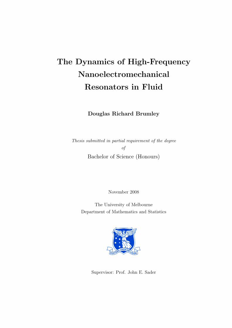
20
The general solution is then
W (x|ω) = A1eχx +B1e
−χx + C1eγix +D1e
−γix,
or equivalently
W (x|ω) = A cosh(χx) +B sinh(χx) + C cos(γx) +D sin(γx),
where A, B, C and D are arbitrary constants. The boundary conditions are precisely
the same as those from Eq. (3.5). Application of such conditions to the above general
solution yields the following dispersion relation:
2 coshχ cos γ +(γ
χ− χ
γ
)sinhχ sin γ − 2 = 0. (3.11)
Equation (3.11) is too complicated to solve analytically, however a suitable software
package such as mathematica R© can easily find numerical solutions. Recall that χ and
γ are functions of both H and σ which are in turn functions of T and ω respectively.
Thus, Eq. (3.11) relates the tension T in the beam with the permissible vibrational
modes. It is important to note that the only difference between solving for the in-plane
modes and the out-of-plane modes lies in the value of I which is different for the two
cases. The intrinsic tension is not something that is generally known given the man-
ufacturing procedure. It is left as a tuneable parameter which must be determined
numerically. The value of T will depend only on the beam itself and not on the nature
of any deflection which it undergoes since it is an inherent property of the material.
The actual resonant frequencies of the blade are well-known. Using Eq. (3.11) it is
possible to solve for the value of H and thus T given the experimental values of ω. If all
aspects of the model are correct and we have not missed anything, then the subsequent
values of T should turn out to be the same in all cases. However, the calculated values
of the parameter T turn out to vary by a factor of approximately 5 over the range of
exhibited vibrational modes. This is hardly surprising given how crude our model is
at this stage. To perform a regression in order to determine an appropriate value of
T is unwarranted, since it is far more likely that there are other aspects of the system
responsible for this behaviour which we have failed to include.

Chapter 3. Resonant Frequencies in Vacuum 21
Based on finite-element simulations performed using femlab, Bargatin et al. [2]
conclude that the 16µm-beam possesses an intrinsic tensile strain of ε = 2.8 × 10⁻⁴
which would correspond to T = Ebhε = 3.85 × 10⁻⁶ N. Using the dispersion relation
that is Eq. (3.11), the values of ω and thus f corresponding to this choice of T can be
found. In Fig. 3.1 we present the predicted resonant frequencies for such a situation
alongside the experimental values.
1 2 3 4 5 6 7 8 9 10 11 1210
0
101
102
103
Mode Number
Fre
quen
cy (
MH
z)
IN−PLANE
OUT−OF−PLANE
ExperimentT = 3.85µNT = 0N
Figure 3.1: Plot of predicted and experimental resonant frequencies for in-plane and out-of-plane modes of 16µm-long beam in vacuum. Free vibrations (dotted); Intrinsic tension T =3.85× 10⁻⁶ N (dashed); Experimental values (solid).
We note that the inclusion of intrinsic tension into the model has a much more
pronounced effect on the out-of-plane modes than on the in-plane modes. Indeed, this
can be accounted for by the fact that in-plane movement of the beam is much stiffer
than out-of-plane motion. Thus, the in-plane modes are less susceptible to changes in
tension of the beam.
The difficulty faced in choosing an appropriate value of T across all modes now
becomes apparent. Increasing the tension in the beam causes a subsequent increase in
the resonant frequency of all modes. If we increase T beyond 3.85 × 10⁻⁶ N in order
to match up the low frequency predictions with experiment, we do so at the expense
of the higher modes. Indeed, it is impossible to find a value of T which yields truly
accurate predictions across the range of exhibited modes. This problem is even more
significant for the out-of-plane modes of the 8µm-long beam, where the predictions for

22
the high and low frequencies (see Table 3.1) are seen to significantly overestimate and
underestimate respectively. Let us not be disheartened by this fact. We have managed
to obtain reasonably accurate estimates of the resonant frequencies given the crudeness
of the model. There are several aspects of the model which must be revisited and
questioned:
• We have assumed that the boundary conditions given in Eq. (3.5) are appropriate
for all modes. It is likely that in the high-frequency regime, the validity of these
boundary conditions becomes questionable. Indeed we must bear in mind that we
are attempting to model a real situation. It is likely that, particularly for higher
frequencies, the beam is subject to imperfect clamping. This would obviously
affect the calculated resonances in a fashion that is non-uniform across the fre-
quency range. Inspection of the data in Tables 3.1 and 3.2 reveals that the error
in our predictions is much more significant for the 8µm-long beam. For the higher
mode numbers, the free vibrating beam model yields substantial overestimates.
It appears that the consequences of imperfect clamping are more pronounced for
the shorter beam.
• The beams used by Bargatin et al. [2] contained gold actuation and gold-palladium
detection loops. These were used to thermally initiate the motion of the blade,
and detect the frequency of vibration respectively. These features mean that the
apparatus is anisotropic. The loops are relatively small, and so the corresponding
effects will be minimal. However, we must acknowledge that the model we have
adopted to predict the resonances does assume isotropy of the beam.
We emphasise that the resonant frequencies predicted in this chapter will not be
used in any of the subsequent chapters. In attempting to predict the quality factors
associated with the in-plane resonances, we will use the actual resonant frequencies
measured by Bargatin et al. [2].

Chapter 3. Resonant Frequencies in Vacuum 23
3.2.1 Euler Buckling Formula
We now seek to verify the Euler formula for column buckling. We know that
applying tension to the beam causes a subsequent increase in the allowable modes of
vibration. Intuition would suggest that if a compressive force was applied, the converse
would happen. For a sufficiently large compressive force, we anticipate that the beam
will buckle. Physically this corresponds to the value of T where the frequency of vi-
bration of the beam approaches zero. Recall the definitions of H and σ from Eq. (3.8).
Close to the onset of buckling we obviously have σ → 0. We can thus consider |H| σ
from now on. We note thatH < 0 since we are considering the beam under compression.
It follows that √H2 + 4σ ≈ −H
(1 +
12
4σH2
). (3.12)
Equations (3.9) and (3.10) thus become
χ ≈√− σ
H, γ ≈
√− σ
H−H.
After substitution of the above equations into Eq. (3.11) and performing a Taylor
series expansion about σ = 0, we see that to leading order,
2 cos√−H +
√−H sin
√−H − 2 = 0. (3.13)
By inspection, solutions to Eq. (3.13) are given by −H = 4π2n2 for n = 1, 2, 3, . . ..
There are many buckling modes possible, but we are primarily interested in the lowest
one, corresponding to n = 1. In this situation,
T = − π2EI
(KL)2,
where we have defined K = 1/2. This corresponds precisely to the buckling formula of
an ideal column.


Chapter 4
High-Frequency Limit
In the limit of high-frequency, oscillations of an infinitely thin blade in the fluid will
generate an extremely thin viscous boundary layer near its surface. In this limit, the
fluid does not see the width or length of the blade. This facilitates the use of an infinite
plate solution. To begin with, let us consider the linearized Navier-Stokes equation.
We justify ignoring the non-linear convective term since for an infinite plate the fluid
exhibits unidirectional flow. In addition, the amplitude of oscillation is considered to
be small (see Section 2.1) and so the non-linear effects are negligible. The governing
equation for the fluid is then∂u
∂t= ν∇2u, (4.1)
where u = uy is the velocity and ν is the kinematic viscosity of the fluid above the
plate. The plate oscillates with angular frequency ω so it is natural to Fourier transform
Eq. (4.1) and work in the frequency domain. We have
−iωU = ν∇2U .
This is an ordinary differential equation for U , and is given by
d2U(z|ω)dz2
= − iωνU(z|ω). (4.2)
25

26
Solving this and requiring that U → 0 as z →∞, we obtain the following general
solution for the fluid velocity above the plate:
U(z|ω) = A exp(i
√iω
νz
). (4.3)
4.1 No-Slip Boundary Condition
If we wish to apply the no-slip boundary condition, we simply identify A in Eq. (4.3)
as the velocity amplitude of the plate. If W (ω) is the displacement amplitude of the
oscillating plate, then A can be written as −iωW (ω). We note that although our
vibrating beam appears locally infinite, the displacement varies along its length. ie.
W = W (x|ω). The fluid velocity above the plate thus becomes
U(x, z|ω) = −iωW (x|ω) exp(i
√iω
νz
). (4.4)
The stress tensor for incompressible flow can be easily calculated and is given by
T = µωW (x|ω)
√iω
ν
(zy + yz
)− µiωdW (x|ω)
dx
(xy + yx
).
The stress vector,
t = n ·T = µωW (x|ω)
√iω
νy,
is the force per unit area exerted by the fluid on the surface, with normal vector n
pointing into the fluid. The net force per unit length on the vibrating blade exerted by
the fluid is then given by
Fhydro = 2bµωW (x|ω)
√iω
ν, (4.5)
where the factor of 2 accounts for the top and bottom faces and b is the width of the
blade. Comparing Eqs. (4.5) and (2.4), we see that
Γ(ω) =8πb
√iν
ω. (4.6)
If λ is the linear mass density of the beam, ρ is the density of the fluid and Γr and
Γi are the real and imaginary components of the hydrodynamic function respectively,

Chapter 4. High-Frequency Limit 27
then the associated quality factor for a given frequency ω is given by Eq. (2.6):
Q =4λπρb2
+ Γr(ω)
Γi(ω)
= 1 +λ
b
√ω
2µρ. (4.7)
There are a couple of interesting points to note from Eq. (4.7). Recall that the
quality factor relates to the rate of energy dissipation from the blade due to viscous
losses. A large quality factor corresponds to a system where such energy losses are
relatively small. For the current system, we note in particular the frequency dependence
of Q. We see that high-frequency modes have relatively large associated quality factors.
Note also that Q is a decreasing function of blade width b and surrounding fluid viscosity
µ and density ρ. This result is in perfect accordance with intuition. It is important
to note that although we have assumed an infinitely thin viscous boundary layer and
used the corresponding infinite plate solution, we have certainly not treated the blade
as an infinite plate itself. Indeed, quantities such as b and λ do not make sense for an
infinitely large surface.
We emphasise that the expression given for the quality factor in Eq. (4.7) is the
contribution from the fluid only. This does not include any intrinsic quality factor
associated with the blade itself.
4.2 Second-Order Slip Boundary Condition
To this point we have treated the fluid surrounding the resonator as continuous
and have thus adopted the no-slip boundary condition at the fluid-blade interface. The
Knudsen number for the 400nm-wide blade in air is Kn ≈ 0.17 and so the use of contin-
uum mechanics near the blade surface is actually inappropriate. Recall the second-order
slip boundary condition presented in Eq. (2.1). We can rewrite this equation in terms
of the Fourier transformed velocity:
U∣∣z=0
− uw = γη∂U
∂z
∣∣∣∣z=0
− δη2 ∂2U
∂z2
∣∣∣∣z=0
, (4.8)
where uw is the velocity of the wall. Observe that the no-slip boundary condition used
previously corresponds precisely to the case where η = 0 m. For one-dimensional flows,

28
the hard-sphere second-order slip model can be used with γ = 1.11 and δ = 0.61. These
parameter values are fixed for the purposes of this section, though we can set δ = 0 to
adopt the first-order slip condition. We begin with the fluid velocity given in Eq. (4.3)
and identify C = i√
iων . For a blade oscillating at angular frequency ω, the wall velocity
is uw = −iωW (x|ω) as before. Equation (4.8) thus becomes
A+ iωW (x|ω) = γηAC − δη2AC2,
and so
A =−iωW (x|ω)
1− γηC + δη2C2. (4.9)
Since the fluid velocity field is known, we can proceed to find the net force per unit
length exerted on the blade by the fluid:
Fhydro = 2bµAC,
or equivalently
Fhydro =π
4ρω2b2Γ(ω)W (x|ω),
where the hydrodynamic function Γ(ω) is given by
Γ(ω) =8νπb
√i
νω× 1
1− γηC + δη2C2(4.10)
=8ν√iν
πb√ω(ν − iγη
√iων − iδη2ω
) . (4.11)
The real and imaginary components of the hydrodynamic function are then
Γr(ω) =4ν
√2νω
(ν − δη2ω)
πb
[ν2 + γην
(γηω +
√2νω
)+ δη3ω
(δηω + γ
√2νω
)] , (4.12)
Γi(ω) =4ν
√νω
[√2ν + η
(√2δηω + 2γ
√νω
)]πb
[ν2 + γην
(γηω +
√2νω
)+ δη3ω
(δηω + γ
√2νω
)] . (4.13)

Chapter 4. High-Frequency Limit 29
4.3 Matched Asymptotic Expansion
We now attempt to calculate explicitly the correction to the no-slip results arising
through inclusion of first-order slip. The two flow regimes are the kinetic layer close to
the beam and the region far away from the beam. We begin by writing the solution as
an asymptotic expansion for small values of the scaled mean free path η = η/a = 2Kn;
U = U (0) + ηU (1) +O(η2) (4.14)
Recall that the Fourier transformed linearized equation of motion of the fluid is
given byd2U
dz2= − iω
νU .
Upon substitution of Eq. (4.14) into the governing equation and equating orders of η,
we see thatd2U (n)
dz2= − iω
νU (n) for n = 0, 1, 2, . . . .
It follows that the general solution for each order of η is the same and is given by
U (n) = An exp(i
√iω
νz
)for n = 0, 1, 2, . . . (4.15)
where An must be determined for each order. The first-order slip condition can be
rewritten as
U (0) + ηU (1) +O(η2) = uw + aγη
(dU (0)
dz+ η
dU (1)
dz+O(η2)
),
where each side of the above equation is evaluated at z = 0. We can equate the
coefficients of different orders of η to obtain the boundary conditions for the different
orders. We find these to be
O(1) : U (0)∣∣z=0
= uw, (4.16)
O(η) : U (1)∣∣z=0
= aγdU (0)
dz. (4.17)
Notice that Eq. (4.16) is quite simply the no-slip boundary condition. To leading
order, the perturbation expansion in η yields the no-slip boundary condition as it should.

30
Furthermore, we note that the right hand side of Eq. (4.17) can be written in terms of
the zeroth-order vorticity. Since dU (0)/dz = −ω(0), Eq. (4.17) becomes
U (1)∣∣z=0
= −aγω(0)∣∣z=0
.
The first-order correction to the fluid velocity can be found using the zeroth-order
solution. The function ω(0) is simply the fluid vorticity at the surface in the no-slip
case, for which which we have already solved. It can be found directly from Eq. (4.4)
and the corresponding boundary condition for the slip velocity becomes
U (1)∣∣z=0
= γaωW (x|ω)
√iω
ν.
Upon application of the above boundary condition, the general solution presented
in Eq. (4.15) yields the slip velocity,
U (1) = γaωW (x|ω)
√iω
νexp
(i
√iω
νz
).
Thus, to first-order in η, the fluid velocity is given by
U = U (0) + ηU (1)
= ωW (x|ω)(− i+ γη
√iω
ν
)exp
(i
√iω
νz
).
Since the fluid velocity field is known, we can proceed to find the net force per unit
length exerted on the blade by the fluid,
Fhydro = 2bµωW (x|ω)(√
iω
ν− γηω
ν
). (4.18)
Notice that if we set η = 0, the force corresponding to the no-slip condition is
indeed recovered as in Eq. (4.5). Furthermore, we see that the inclusion of slip serves
to reduce the force exerted on the blade by the fluid; a mathematical result consistent
with our intuition. We can evaluate the hydrodynamic function associated with the slip
case by equating Eq. (2.4) and Eq. (4.18). We see that
Γ(ω) =8πb
(√iν
ω− γη
). (4.19)

Chapter 4. High-Frequency Limit 31
This solution is only appropriate for η 1 (or equivalently Kn 1). We note that
the first-order correction to the hydrodynamic function is actually quite large. Indeed,
unphysical solutions can be obtained for fairly modest values of Kn. We know that as
Kn →∞, the force should approach zero and so Γ → 0 in this limit. In order to satisfy
this condition, we construct a Pade approximant [12] from Eq. (4.19) by noting that
1− x ≈ 11+x for small x. This can be written as
Γ(ω) =8πb
√iν
ω
(1− γbKn
√ω
iν
)
≈8πb
√iνω
1 + γbKn√
ωiν
. (4.20)
For Kn 1, Eqs. (4.19) and (4.20) have the same asymptotic form, whilst the
latter has the advantage of also possessing the correct asymptotic form as Kn →∞. In
fact, for large Kn, Eq. (4.20) becomes
Γ(ω) ∼ 8νiπγωb2Kn
for Kn →∞.
This is precisely the same form as Eq. (4.10) for large Kn (with δ = 0). We now
plot the solutions in Eqs. (4.19) and (4.20) which have been obtained through matched
asymptotic expansion, alongside the hydrodynamic function in Eq. (4.10) which was
derived using the Navier slip condition. We note that although the second-order slip
condition was used in Section 4.2, we use this solution with δ = 0 to recover the first-
order solution.
Very interestingly, the matched asymptotic expansion initially derived for small Kn
and subsequently modified to give the appropriate behaviour at Kn → ∞, agrees per-
fectly with the results obtained through simple application of the Navier slip condition.
Another interesting feature of Fig. 4.1 is that the first-order correction for small Kn
diverges rapidly from the exact solution as Kn increases. It follows that this expansion,
depicted by the dashed line, is only valid for quite small Kn. Indeed, for the fundamen-
tal mode of the 16µm-long beam used by Bargatin et al. [2], we have Kn ≈ 0.17. Even
for this value the accuracy of the first-order correction has deteriorated.

32
Pade approximantAsymptotic
expansion
for Kn<<1
0.0 0.5 1.0 1.5 2.0 2.5 3.00.0
0.5
1.0
1.5
2.0
Kn
Re@GD
(a)
Asymptotic
expansion
for Kn<<1
Pade approximant
0.0 0.2 0.4 0.6 0.8 1.00.0
0.5
1.0
1.5
2.0
Kn
Im@GD
(b)
Figure 4.1: Real and imaginary components of the hydrodynamic function for the fundamentalmode of the 16µm-long beam used by Bargatin et al. [2]. The plots show the matched asymptoticexpansion (dashed) and modified asymptotic expansion (solid). The latter coincides perfectlywith the results from Section 4.2 where the Navier slip condition was used.

Chapter 4. High-Frequency Limit 33
4.4 Progressive Comparison With Experiment
We emphasise that for the thin boundary layer approximation, Q does not depend
on the length of the blade being considered, nor on the shape of the mode. The width of
the blade and the material properties of both the blade and surrounding fluid influence
Q, but these are fixed across the range of beams used by Bargatin et al. [2]. The
quality factor is thus a function only of frequency. We now present the calculated
quality factors alongside the experimental values. Note that the experimental quality
factors presented here correspond to the fluid contribution only.
Experiment Theoryβ Qfluid only Qno-slip Qfirst-order slip Qsecond-order slip
0.3527 136 448 465 4590.9223 339 721 783 7681.7477 535 996 1141 11192.8268 804 1268 1537 15234.1315 1160 1529 1960 19770.4346 157 497 519 5120.8115 311 678 731 717
Table 4.1: Quality factors predicted by infinitely thin boundary layer model for first five in-plane resonances of 16µm-long beam and second and third in-plane resonances of 24µm-longbeam.
The frequencies used to predict the quality factors are the actual resonant fre-
quencies and not the values presented in Chapter 3. From Table 4.1, we see that the
predicted values are significantly higher than the experimental quantities. In accordance
with intuition, incorporating the effects of slip increases the calculated quality factors.
Notice also that the effect of slip is more pronounced in the high-frequency regime as
Qno-slip and Qslip begin to diverge. In addition, Qfirst-order slip > Qsecond-order slip for low
frequencies and Qfirst-order slip < Qsecond-order slip for high frequencies. Indeed, consider
the following plot, which shows the predicted and experimentally determined quality
factors.

34
æ
æ
æ
æ
æ
+
+
Second- order slip
No - slip
First- order slip
Experiment
10 50 100 500 1000 5000f HMHzL10
100
1000
104
Q
Figure 4.2: Infinitely thin boundary layer model : Predicted and experimental quality factors.No-slip (solid), first-order slip (dashed) and second-order slip (dotted) results are depictedalongside experiment values for the 16µm-long (dots) and 24µm-long (+) beams.

Chapter 5
Beam of Zero Thickness
So far we have considered the beam to be infinitely thin, and have associated with
it an infinitely thin boundary layer, thereby neglecting any edge effects. We now explore
the case where we have a blade of finite width. In order to do so we will adopt and
extend the boundary integral technique of Tuck [5]. Furthermore, we will again employ
the second-order slip model and examine the consequences in terms of the calculated
quality factors.
ω(y,0+)
−a a
ω(y,0-)
y
z
Figure 5.1: Cross-section of beam of zero thickness
35

36
We consider an infinitely thin beam, the length of which greatly exceeds its width.
To justify ignoring the non-linear convective term in the equation of motion of the fluid,
we insist that the amplitude of oscillation of the blade is extremely small; a condition
which is typically satisfied during experiment [3]. It then follows that the fluid velocity
has components only in the y and z directions (refer to Figs. 1.2 and 5.1 for orientation
of coordinate axes). It follows that u = vy +wz where v and w are the components of
the fluid velocity in the y and z directions respectively. Since the fluid velocity in the
x direction vanishes, i.e. u = 0, we can express the fluid vorticity as
ω =(∂w
∂y− ∂v
∂z
)x− ∂w
∂xy +
∂v
∂xz.
The vorticity above and below the oscillating blade can be written as
ωtop =(∂wtop
∂y− ∂vtop
∂z
)x− ∂wtop
∂xy +
∂vtop∂x
z, (5.1)
ωbottom =(∂wbottom
∂y− ∂vbottom
∂z
)x− ∂wbottom
∂xy +
∂vbottom
∂xz. (5.2)
However, by symmetry, Eq. (5.2) becomes
ωbottom =(∂wtop
∂y+∂vtop∂z
)x− ∂wtop
∂xy +
∂vtop∂x
z. (5.3)
It then follows that the vorticity difference across the face of the blade is given by
∆ω = ωtop
∣∣z=0+ − ωbottom
∣∣z=0−
= −2∂vtop∂z
∣∣∣∣z=0
x. (5.4)
Since the vorticity jump has a non-zero component only in the x-direction, we will
abandon the vector notation and proceed to write it as ∆ω(x, y), i.e. ∆ω = ∆ω(x, y)x.
For the long, infinitely thin blade with cross-section from (y, z) = (−a, 0) to (a, 0), we
can also write the pressure difference across the face of the blade as
∆p(x, y) = p(x, y, z)∣∣z=0+ − p(x, y, z)
∣∣z=0−
. (5.5)

Chapter 5. Beam of Zero Thickness 37
Tuck [5] showed that for a cylinder of arbitrary cross-section undergoing sufficiently
small oscillations, the two-dimensional streamfunction can be written as
ψ =∫C
[ψGn − ψnΩ− ωΨn +
1µpΨl
]dl, (5.6)
provided the pressure p is continuous on the cross-section contour C. In the above
equation, ∂/ ∂l and ∂/ ∂n represent the derivatives tangential and normal to C, re-
spectively, and ω is the fluid vorticity. The streamfunction ψ satisfies the equation
∇4ψ = α2∇2ψ. The function Ψ is the corresponding Green’s function for this equation
and thus satisfies ∇4Ψ− α2∇2Ψ = δ. Tuck [5] gives the solution to this equation as
Ψ = − 12πα2
(logR+K0(αR)),
where K0 is the modified Bessel function of the third kind, zeroth-order. In the above
equation, α2 = iων and R =
√(y − y′)2 + (z − z′)2. We note that α has dimensions of
inverse length. In order to satisfy the requirement that the arguments of the transcen-
dental functions are dimensionless, we rewrite Ψ as
Ψ = − 12πα2
(log (αR) +K0(αR)
).
This is a minor modification to Tuck’s expression, and has no bearing on the
calculated results since the factor disappears upon differentiation of Ψ. Nevertheless,
for consistency we proceed with the latter expression. Recall that ν is the kinematic
viscosity of the surrounding fluid and ω is the angular frequency at which the cylinder
oscillates. It is important not to confuse this angular frequency with the vorticity in
Eq. (5.6). We also have
G =12π
log(αR),
Ω = − 12πK0(αR),
where ∇2Ω − α2Ω = δ(y − y′)δ(z − z′) and Ψ = 1α2 (Ω − G). The Green’s function
G satisfies Laplace’s equation in two dimensions, i.e. ∇2G = δ(y − y′)δ(z − z′). In
the above equation we have inserted a factor of α in the expression for G in order to
maintain dimensional integrity. For the infinitely thin blade, Tuck [5] showed that the

38
two-dimensional streamfunction presented in Eq. (5.6) reduces substantially to become
ψ(y′, z′) =∫ a
−a
[∆ω(y)Ψz(y, 0; y′, z′)− 1
µ∆p(y)Ψy(y, 0; y′, z′)
]dy. (5.7)
One subtlety that is not mentioned by Tuck is that the above expression is only
valid when the streamfunction is evaluated away from the surface of the cylinder. In
evaluating ψ(y′, z′) at the surface, there exists a factor of one half. This is a direct
consequence of a Dirac delta function being “split in half” when a volume integral is
evaluated during the derivation. Thus, Eq. (5.6) should actually read
On contour C :12ψ(y′, z′) =
∫C
[ψGn − ψnΩ− ωΨn +
1µpΨl
]dl, (5.8)
Off contour C : ψ(y′, z′) =∫C
[ψGn − ψnΩ− ωΨn +
1µpΨl
]dl. (5.9)
In the subsequent sections and chapters we will be required to take derivatives of
ψ with respect to both the normal and tangential coordinates to the surface of C. In
evaluating ψl and ψn, we will use Eqs. (5.8) and (5.9) respectively. If the surface C is
a streamline, then the factor of 1/2 will not contribute at all since it will only manifest
itself in ψl = 0, in which case it can be removed.
5.1 No-Slip Boundary Condition
For the infinitely thin blade immersed in a viscous fluid and subject to the no-slip
boundary condition, the fluid velocity calculated using the streamfunction in Eq. (5.7)
must match the blade velocity at the surface. From Eq. (5.7), it is easy to show
that the normal and tangential oscillations of the blade are uncoupled, and that the
two components of the motion of the blade can be expressed as the following integral
equations:
ψ(y′, 0) = − 1µ
∫ a
−a∆p(y)Ψy(y, 0; y′, 0)dy, (5.10)
U(y′) = ψz′(y′, 0) =∫ a
−a∆ω(y)Ψzz′(y, 0; y′, 0)dy. (5.11)
Note that we are considering the cross-section of the blade at a fixed value of x.
Thus, Eqs. (5.10) and (5.11) are independent of x. We will consider the x-direction
later, however for the time being, we restrict ourselves to motion in the y − z plane.

Chapter 5. Beam of Zero Thickness 39
We are particularly interested in the tangential component of the blade’s velocity since
we are considering the in-plane modes. The Green’s function Ψ is known, so we can
directly evaluate Ψzz′(y, 0; y′, 0).
Ψz =∂Ψ∂z
=dΨdR
× ∂R
∂z,
Ψzz′ =∂
∂z′
(dΨdR
∂R
∂z
),
=(dΨdR
)(∂2R
∂z ∂z′
)−
(d2ΨdR2
)(∂R
∂z
)2
.
Upon setting z = z′ = 0, the second term vanishes and
∂2R
∂z ∂z′
∣∣∣∣z=z′=0
=−1√
(y − y′)2=
−1|y − y′|
.
We can then write
Ψzz′(y, 0; y′, 0) =−1
|y − y′|dΨdR
∣∣∣∣z=z′=0
.
Let Z = αR∣∣z=z′=0
= α|y − y′|. The above equation becomes
Ψzz′(y, 0; y′, 0) =1
2πZd
dZ
(log (Z) +K0(Z)
).
If we define the kernel function as
L(Z) =1
2πZd
dZ
(logZ +K0(Z)
),
then our integral equation becomes
U(y′) = ψz′(y′, 0) =∫ a
−a∆ω(y)L(α|y − y′|)dy. (5.12)
We would now like to consider the behaviour of L(Z) for small and large values of Z:
L(Z) = − 14π
(logZ + γ − 1
2− log 2
)+O(Z2) for Z 1, (5.13)
L(Z) =1
2πZ2− 1√
8πZe−Z
(1Z
+O(
1Z2
))for Z 1, (5.14)
where γ is Euler’s constant and is approximately equal to 0.5772. You can see from

40
Eq. (5.13) that the kernel function has a logarithmic singularity for small values of the
argument, i.e. as Z → 0, L(Z) ∝ logZ. Remember that Z = α|y − y′| and so the
logarithmic singularity will need to be acknowledged and treated with care for y ≈ y′.
The equation to be solved is (5.12). Before we proceed, it is a good idea to scale the
problem through the introduction of dimensionless parameters. We know that the cross-
section of the blade is simply the line joining (y, z) = (−a, 0) to (a, 0). The natural
length scale is thus a, and so we scale position across the blade as
ξ =y
a. (5.15)
We also introduce the dimensionless frequency and vorticity as
β =ωa2
ν, (5.16)
Λ(ξ) =(a
U0
)∆ω(y). (5.17)
We will consider the long-term behaviour of the system only. After the transients
have died away, the vorticity jump due to U(y)e−iωt is ∆ω(y)e−iωt where U and ∆ω
are related through Eq. (5.12). For this case, we take U(y) = U0 = constant. Thus,
Eq. (5.12) becomes
U0e−iωt =
∫ a
−a∆ω(y)e−iωtL(α|y − y′|)dx,
which simplifies substantially once the scaled variables are introduced to become∫ 1
−1Λ(ξ)L(−i
√iβ|ξ − ξ′|)dξ = 1. (5.18)
5.1.1 Numerical Solution Method
We know the kernel function L and wish to solve for the complex-valued vorticity
distribution Λ(ξ). We cannot solve the integral equation (5.18) analytically and so will
seek a numerical solution. This will involve discretizing the domain ξ ∈ [−1, 1]. The
integral equation (5.18) can then be transformed into a summation using an appropriate
quadrature method. The corresponding matrix-vector equation that will eventuate from
this process can then be easily solved. Before we attempt to solve Eq. (5.18), there are
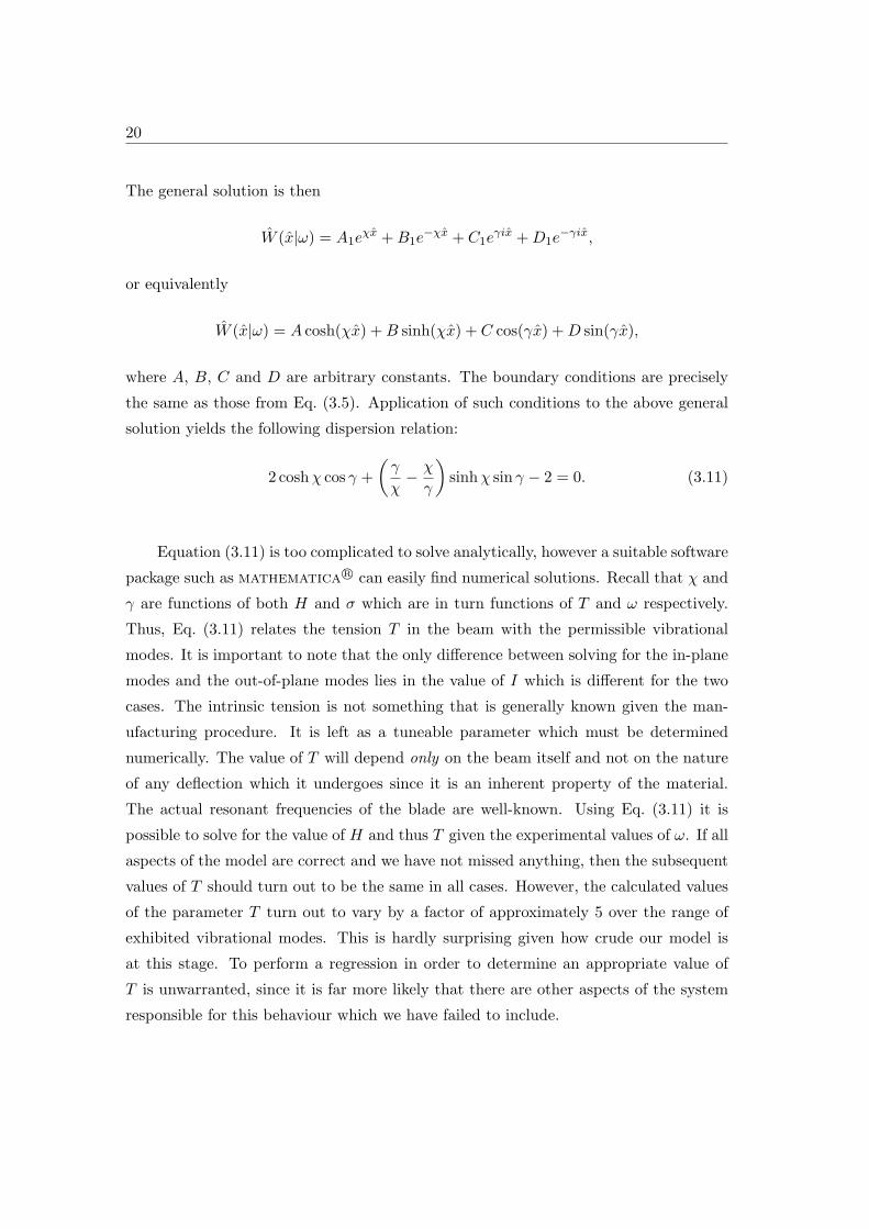
Chapter 5. Beam of Zero Thickness 41
a few concerns which must first be addressed:
1. The presence of the logarithmic singularity in the kernel function at ξ = ξ′.
2. The blade under consideration is infinitely thin. At the leading edges, we expect
the presence of a square-root singularity [5]. That is, we anticipate square-root
singularities in Λ(ξ) at ξ = ±1.
3. Consider the exponential term in Eq. (5.14). If β is large, then this term oscillates
rapidly as it approaches zero.
These are the same issues that Tuck [5] faced in solving the case of normal oscil-
lations. However, we will see that these sources of potential problems can be resolved
quite easily. The presence of the logarithmic singularity in the kernel function will ac-
tually turn out to be beneficial. As a result of the singularity, the kernel matrix that
will be formed once an appropriate quadrature rule is decided upon will be diagonally
dominant, and hence easy to invert [5]. The square-root singularity in Λ(ξ) can be
easily accounted for by taking unequal intervals in the quadrature formula, with a bias
towards the ends. We know that the vorticity will exhibit a square-root singularity at
the edges of the blade. Though an accurate numerical solution can be found by breaking
up the interval ξ ∈ [−1, 1] evenly, into many pieces, the convergence would be slow and
would require N to be very large indeed. It is much more efficient to break up the inter-
val using the points ξ = ξj = − cos(πjN
), j = 0, . . . , N . The third issue can be resolved
by observing that we do not expect Λ(ξ) to vary significantly. We will approximate
Λ(ξ) as a constant on each interval, but will not approximate the kernel function L in
the quadrature method. Using Eq. (5.18) and approximating Λ(ξ) = Λj = constant on
each interval ξj < ξ < ξj+1, we obtain the following equation:
N−1∑j=0
(Λj
∫ ξj+1
ξj
L(−i√iβ|ξ − ξ′|)dξ
)= 1. (5.19)
We then demand that Eq. (5.19) hold at the mid-point of each segment. In other
words, we set ξ = ξ′k = 12(ξk + ξk+1) for k = 0, 1, . . . , N − 1 and substitute this into
Eq. (5.19). This yields
N−1∑j=0
(Λj
∫ ξj+1
ξj
L(−i√iβ|ξ − ξ′k|)dξ
)= 1 k = 0, 1, . . . , N − 1. (5.20)

42
Equation (5.20) can actually be expressed as the following matrix equation:
N−1∑j=0
MkjΛj = 1, k = 0, 1, . . . , N − 1, (5.21)
where
Mkj =∫ ξj+1
ξj
L(−i√iβ|ξ − ξ′k|)dξ. (5.22)
Since the kernel function L is known, we can evaluate the N ×N matrix M . Aside
from N , the matrix M will depend solely on β, the dimensionless frequency defined
in Eq. (5.16). Constructing this matrix is relatively straightforward using a software
package such as mathematica R© . Once this is done, the matrix-vector system can
be solved. We note that the solutions can be found by built-in linear solvers or by
direct inversion of the matrix M . Both methods yield the same results, though from
a computational point of view, the former method is more robust. We readily find the
vector Λ containing the numerical solutions Λj at each of the points ξ′j . Since we have
discretized the problem by turning the integral equation into a matrix-vector equation,
we cannot find a continuous solution for Λ(ξ). However, increasing N will increase the
number of computed points. Obviously, N must be sufficiently large so as to ensure
that any numerical solution which is obtained is accurate. We will consider this in more
depth shortly.
Recall that Λ(ξ) = Λj has been treated as constant on each of the intervals ξj <
ξ < ξj+1. Λ(ξ) is a complex-valued function and so in plotting it over the appropriate
domain, we must consider both its real and imaginary components. Below is a plot of
the vorticity distribution for the first in-plane resonance of the blade of length 16µm.
The only independent variable that explicitly determines the shape of this graph is the
frequency of oscillation of the blade.

Chapter 5. Beam of Zero Thickness 43
−1 −0.8 −0.6 −0.4 −0.2 0 0.2 0.4 0.6 0.8 1−6
−4
−2
0
2
4
6
8
10
Position ξ
Vor
ticity
Λ(ξ
)
Re(Λ(ξ))
Im(Λ(ξ))
Figure 5.2: Vorticity difference across the infinitely thin blade subject to no-slip boundarycondition. β = 0.3527, N = 60.
5.1.2 Calculation of Hydrodynamic Function
We have found that the complex-valued vorticity distribution is a function of both
frequency and position, i.e. Λ = Λ(ξ, β). However, we do not have an analytic expres-
sion for Λ directly. It is very important to note that at this stage, the vorticity profile is
known across the face of the blade for a given velocity amplitude U0. As of yet, we do
not know how it varies along the length of the beam. Ultimately, we seek to know the
frequency dependence of the quality factors associated with this beam. Recall Eq. (5.4),
where we obtained an expression for the vorticity difference across the surface of the
blade. The stress tensor for incompressible flow is given by
T = 2µe = µ
(∇u + (∇u)T
). (5.23)

44
The stress vector,
t = n ·T, (5.24)
is the force per unit area exerted by the fluid on the surface, with normal vector n
pointing into the fluid. Recall that the fluid velocity can be written as u = vy + wz.
Combining this with Eqs. (5.23) and (5.24), the component of the stress vector in the
y-direction for the two faces of the blade can be written as
ttop · y =(z ·Ttop
)· y,
tbottom · y =(− z ·Tbottom
)· y.
The total pressure exerted on the blade in the y-direction is then given by
t · y =(ttop + tbottom
)· y,
which simplifies substantially to become
t · y = 2µ∂vtop∂z
∣∣∣∣z=0
= −µ∆ω(x, y).
We are considering motion where the velocity amplitude is U0. Earlier we solved for
the complex vorticity in 2-dimensions, namely the y-z plane. We introduced a velocity
amplitude U0 that was taken to be constant in y. Now that we extend this problem to
3-dimensions, we need to account for the fact that the velocity amplitude of the beam
is actually a function of x. We know that U(x, t) = U0(x)e−iωt, and so
U0(x) = −iωW (x|ω), (5.25)
where W (x|ω) is the displacement amplitude as a function of distance x along the
beam. We can write the net force per unit length that the fluid exerts on the beam in
the y-direction as
Fhydro(x|ω) = −∫ 1
−1µU0(x)Λ(ξ, β)dξ. (5.26)

Chapter 5. Beam of Zero Thickness 45
Substituting Eq. (5.25) into Eq. (5.26) yields
Fhydro(x|ω) = µiωW (x|ω)J(ω), (5.27)
where J(ω) =∫ 1−1 Λ(ξ, β)dξ has been written as a function of the dimensional frequency
ω rather than the scaled frequency β. In calculating the integral J(ω), we use the
midpoint rule given by
J(ω) =∫ 1
−1Λ(ξ, β)dξ ∼
N−1∑j=0
Λj(ξj+1 − ξj
). (5.28)
We see from Eq. (5.27) that the hydrodynamic force on the blade at position x is
proportional to the displacement amplitude of the blade at that point. In addition, the
frequency dependence manifests itself in two different ways. Firstly, in the mode shape
W (x|ω) as just mentioned. For larger amplitude of vibration, the force will be larger.
Secondly, the term J(ω) is simply the integral of the complex vorticity difference over the
width of the blade. Something which is important to note is that J(ω) knows nothing
about the in-plane resonances of the blade. All information regarding the resonances is
encompassed in the term W (x|ω). Now that an expression for the hydrodynamic force
on the blade has been found, the hydrodynamic function can be calculated. Equating
Eqs. (2.4) and (5.27), we see that
µiωW (x|ω)J(ω) =π
4ρω2b2Γ(ω)W (x|ω). (5.29)
The displacement function cancels from both sides and so the hydrodynamic func-
tion will depend only on the frequency of oscillation of the blade and not on the mode
shape explicitly. We will find that the quality factors associated with the oscillations
are also independent of W (x|ω). From Eq. (5.29) the hydrodynamic function can be
written as
Γ(ω) =4µiπρωb2
J(ω) =i
πβJ(ω). (5.30)
The real and imaginary components of the hydrodynamic function represent the
added mass of the beam and the viscous losses respectively. In modelling the interaction
of the blade with the fluid, we have assumed zero thickness. However, it is important
to realise that the beam still has a non-zero linear mass density.

46
5.2 Second-Order Slip Boundary Condition
Recall the expression for the two-dimensional streamfunction in Eq. (5.7). For
in-plane modes, ∆p(y) = 0 by symmetry and so
ψ(y′, z′) =∫ a
−a
[∆ω(y)Ψz(y, 0; y′, z′)
]dy.
The Green’s function Ψ is analytic everywhere in the y-z plane except at y = y′,
z = z′. For this reason, we avoid setting z′ = 0, but work very close to this limit. The
fluid velocity and its first two derivatives with respect to the normal coordinate are
given by
U(y′, z′) = ψz′(y′, z′) =∫ a
−a∆ω(y)Ψzz′(y, 0; y′, z′)dy,
∂U
∂z′(y′, z′) = ψz′z′(y′, z′) =
∫ a
−a∆ω(y)Ψzz′z′(y, 0; y′, z′)dy,
∂2U
∂z′2(y′, z′) = ψz′z′z′(y′, z′) =
∫ a
−a∆ω(y)Ψzz′z′z′(y, 0; y′, z′)dy.
Recall from Eq. (2.1) that the second-order slip boundary condition at the surface
of the blade is of the form
U∣∣wall
− uw = γη∂U
∂z′
∣∣∣∣wall
− δη2 ∂2U
∂z′2
∣∣∣∣wall
. (5.31)
Recall also that γ = 1.11 and δ = 0.61 are dimensionless parameters for one-
dimensional flows with hard-spheres. The molecular mean free path is given by η and
uw is the velocity of the blade surface. The physical length scale for the infinitely thin
blade is simply the width of the blade b = 2a. Since we are working in the regime where
the Knudsen number, Kn = η2a ≈ 0.17 < 1, we apply the second-order slip condition in
Eq. (5.31) at the surface of the blade. This is given by
uw = U∣∣wall
− γη ∂U∂z′
∣∣∣∣wall
+ δη2 ∂2U
∂z′2
∣∣∣∣wall
=∫ a
−a∆ω(y)
[Ψzz′(y, 0; y′, z′)− γηΨzz′z′(y, 0; y′, z′) + δη2Ψzz′z′z′(y, 0; y′, z′)
]dy.
(5.32)

Chapter 5. Beam of Zero Thickness 47
We wish to evaluate the above equation at z′ = 0. However, since the Green’s
function Ψ is not analytic at this point, we instead choose to evaluate Eq. (5.32) at
z′ = ε, 0 < ε 1. That is, we proceed to calculate the fluid velocity and its subsequent
derivatives just above the surface of the blade. We scale η according to
η =η
a= 2×Kn,
where Kn is the Knudsen number for the system. The dimensionless frequency β is
defined as earlier,
β =ωa2
ν.
The tangential and normal coordinates can be scaled as
ξ =y
a, ξ′ =
y′
a, χ =
z
a, χ′ =
z′
a.
Since α has dimensions of inverse length, it seems natural to want to scale it to become
dimensionless. Since α2 = iω/ν = iβ/a2, we define
α2 = a2 × α2 = iβ,
and so
α = −i√iβ.
The Green’s Function Ψ thus can be written as
Ψ = − a2
2πα2(log (αR/a) +K0(αR/a)). (5.33)
Then, the dimensionless Green’s Function is
Ψ(κ) =Ψa2
= − 12πα2
(log (ακ) +K0(ακ)
). (5.34)
Scaling Eq. (5.32) in the same fashion as in Section 5.1 and identifying the kernel
function as
L(ξ, 0; ξ′, χ′) = Ψχχ′(ξ, 0; ξ′, χ′)− 2γKnΨχχ′χ′(ξ, 0; ξ′, χ′) + 4δKn2Ψχχ′χ′χ′(ξ, 0; ξ′, χ′),
(5.35)

48
we see that ∫ 1
−1Λ(ξ)L(ξ, 0; ξ′, χ′)dξ = 1. (5.36)
5.2.1 Numerical Solution Method
The complex vorticity distribution is given by Λ(ξ) =(aU0
)∆ω(y). In solving
Eq. (5.36), we will need to take a sufficiently small χ′ > 0 to accurately capture the
behaviour at the surface of the blade. Before we solve this integral equation, there are
several important points which must be raised. The kernel function is comprised of
various derivatives of the Green’s function Ψ, which has a singularity at R = 0. This
seems concerning upon first glance, however this property will actually work to our
advantage. The presence of this singularity will ensure that the kernel matrix obtained
after discretization will be diagonally dominant and thus relatively easy to invert. In
the discretization of Eq. (5.36) we will again use the Chebyshev points defined by
ξ = ξj = − cos(πjN ), j = 0, . . . , N.
Armed with the same tools used for the no-slip case, we attack Eq. (5.36) and
obtain the following matrix-vector equation:
N−1∑j=0
MkjΛj = 1, k = 0, 1, . . . , N − 1,
where
Mkj =∫ ξj+1
ξj
L(ξ, 0, ξ′k, χ′)dξ.
The values Λj correspond to the complex vorticity which is taken to be constant
in each region ξ ∈ [ξj , ξj+1]. The points ξ′k = 12(ξk + ξk+1) are the midpoints of each
domain element. The resultant matrix equation can be constructed and solved quite
easily using mathematica R© . Recall that when the no-slip condition was used, the
corresponding matrix equation had a dependence only on dimensionless frequency β.
However, since the first and second-order slip conditions manifest themselves through
incorporation of the mean free path of the surrounding fluid, the system is no longer
independent of scale. That is, the absolute width of the blade is now significant, as
evident in the dependence of Eq. (5.35) on Knudsen number.
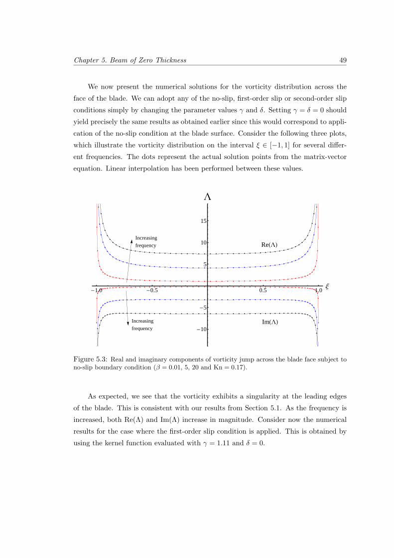
Chapter 5. Beam of Zero Thickness 49
We now present the numerical solutions for the vorticity distribution across the
face of the blade. We can adopt any of the no-slip, first-order slip or second-order slip
conditions simply by changing the parameter values γ and δ. Setting γ = δ = 0 should
yield precisely the same results as obtained earlier since this would correspond to appli-
cation of the no-slip condition at the blade surface. Consider the following three plots,
which illustrate the vorticity distribution on the interval ξ ∈ [−1, 1] for several differ-
ent frequencies. The dots represent the actual solution points from the matrix-vector
equation. Linear interpolation has been performed between these values.
ReHLL
ImHLL
Increasing
frequency
Increasing
frequency
-1.0 -0.5 0.5 1.0Ξ
-10
-5
5
10
15
L
Figure 5.3: Real and imaginary components of vorticity jump across the blade face subject tono-slip boundary condition (β = 0.01, 5, 20 and Kn = 0.17).
As expected, we see that the vorticity exhibits a singularity at the leading edges
of the blade. This is consistent with our results from Section 5.1. As the frequency is
increased, both Re(Λ) and Im(Λ) increase in magnitude. Consider now the numerical
results for the case where the first-order slip condition is applied. This is obtained by
using the kernel function evaluated with γ = 1.11 and δ = 0.

50
Increasing
frequency
ImHLLIncreasing
frequency
ReHLL
-1.0 -0.5 0.5 1.0Ξ
-2
2
4
L
Figure 5.4: Real and imaginary components of vorticity jump across the blade face subject tofirst-order slip condition (β = 0.01, 5, 20 and Kn = 0.17).
Qualitatively, Fig. 5.4 is very different to Fig. 5.3. We note that the vorticity is
not as strongly peaked at the leading edges of the blade. Indeed, the singularities at
ξ = ±1 have been removed. Vorticity is a measure of the average local angular velocity
of a fluid element. This rotational motion is initiated through the tangential motion of
the blade. By incorporating the effects of slip into our model, we diminish the ability
of the blade to introduce vorticity into the surrounding fluid. In addition, note that
in Fig. 5.4, |Im(Λ)| does not increase monotonically with frequency like in Fig. 5.3.
Consider now the effects of adopting the second-order slip boundary condition, which
is done by taking γ = 1.11 and δ = 0.61.

Chapter 5. Beam of Zero Thickness 51
Increasing
frequency
ImHLL
ReHLL
-1.0 -0.5 0.5 1.0Ξ
-1
1
2
3L
Figure 5.5: Real and imaginary components of vorticity jump across the blade face subject tosecond-order slip condition (β = 0.01, 0.2, 5 and Kn = 0.17).
The second-order slip condition has quite a profound effect on the subsequent
vorticity distribution. As a result of the increased slip at the surface of the blade, we
see that the vorticity at the leading edges is very small indeed.
5.2.2 Calculation of Hydrodynamic Function
We now turn our attention to the calculation of the hydrodynamic function associ-
ated with the various in-plane resonances. Recall from Eq. (5.30) that the hydrodynamic
function can be written as
Γ(ω) =i
πβJ(ω),
where we have defined
J(ω) =∫ 1
−1Λ(ξ, β)dξ.
We can use this same equation, since the incorporation of slip affects only the value
of J(ω). The hydrodynamic function can be readily computed for different frequencies.
As in the no-slip case, we evaluate J(ω) using the midpoint rule given in Eq. (5.28).
The real and imaginary components of the hydrodynamic function can be compared

52
for the three cases that we are considering. We will examine the behaviour of such
functions in both the high-frequency and low-frequency regimes.
10−1
10010
−2
10−1
100
101
102
Dimensionless Frequency β
Re(
Γ)
2nd order slip
No−slip
1st order slip
(a)
10−4
10−3
10−2
10−1
100
10110
−2
10−1
100
101
102
103
104
105
Dimensionless Frequency β
Im(Γ
)
2nd order slip
1st order slipNo−slip
(b)
Figure 5.6: (a) Real and (b) imaginary components of hydrodynamic function

Chapter 5. Beam of Zero Thickness 53
From Fig. 5.6, it can be seen that the hydrodynamic functions for each of the three
cases agree in the low frequency limit. From Eq. (5.31), we see that the first and second-
order effects of slip depend on the first and second derivatives of the fluid velocity with
respect to the normal coordinate. For low frequencies, we expect that these derivatives
will be smaller in magnitude and thus the corresponding terms in Eq. (5.31) will be less
significant. In the high-frequency regime, the thickness of the viscous boundary layer
decreases. This becomes the characteristic length scale and so the appropriate Knudsen
number is quite large. Since the second-order slip model works only for Kn < 1 [9],
we see that it can be no longer applied in the high-frequency limit. This is precisely
the reason why the curves in Fig. 5.6 begin to diverge at β ≈ 1. In fact, Im(Γ) < 0
for β > 15 in the second-order slip case. This is clearly unphysical since it would
suggest that the viscous “losses” are negative. We attribute this inconsistency to the
breakdown of the model for large Kn. For high frequencies, the viscous penetration
depth diminishes and so the effective Knudsen number increases.
5.3 Alternative Solution Method for First-Order Slip
As a small aside, we present an alternative method for finding the vorticity distri-
bution across the blade face where the fluid velocity is subject to the first-order Navier
slip condition. Recall this boundary condition is of the form
U∣∣wall
− uw = γη∂U
∂z′
∣∣∣∣wall
,
and can be written in terms of the streamfunction ψ(y′, z′),
∂ψ
∂z′− γη ∂
2ψ
∂z′2= uw. (5.37)
The general form of the streamfunction is known and is presented as a bound-
ary integral in Eq. (5.7). For in-plane modes, the pressure contribution vanishes by
symmetry and we are left with
ψ(y′, z′) =∫ a
−a∆ω(y)Ψz(y, 0; y′, z′)dy. (5.38)

54
The approach in Section 5.2 was to substitute Eq. (5.38) into Eq. (5.37) and rear-
range to obtain an integral equation with the unknown ∆ω(y) located entirely inside
the integrand. While this is an effective method and indeed is necessary to solve for
the second-order slip boundary condition, it is possible to be much more efficient in the
case of first-order slip. Construction of the kernel functions in the previous section is
computationally demanding since the introduction of slip introduces additional terms
into the integral equation. Notice that Eq. (5.37) involves ∂2ψ∂z′2 . Instead of differentiat-
ing Eq. (5.38) twice to obtain this term, we note that it can be written in terms of the
primary unknown. The vorticity on the top face of the blade is ω(y′) = − ∂2ψ∂z′2 and so
combining Eqs. (5.37) and (5.38), we see that[ ∫ a
−a∆ω(y)Ψzz′(y, 0; y′, z′)dy
]+
12γη∆ω(y′) = uw.
The factor of 1/2 accounts for the fact that we are solving for the vorticity difference
across the face of the blade. Upon scaling and discretization of the integral in the same
way as Section 5.2, we obtain the following matrix-vector equation
(M +
12γηI
)Λ =
1
1...
1
, (5.39)
where M is precisely the same matrix as in Eq. (5.21) and I is the N × N identity
matrix. The beauty of using Eq. (5.39) to solve for the first-order slip case is that it is
computationally inexpensive. The only modification necessary from the no-slip case is
the inclusion of some constants to the diagonal elements of the matrix M . Furthermore,
these terms serve to make the matrix even more diagonally dominant and thus more
docile in its inversion properties. The results obtained using this method agree perfectly
with the results from Section 5.2 and so we need not present them.
It must be noted that this method of solving for the vorticity distribution only
works for the first-order slip scenario since ∂2ψ∂z′2 = −ω(y′). In the case of second-order
slip this process cannot be adopted since we cannot write ∂3ψ∂z′3 in terms of the vorticity.
Nevertheless, the approach used in this section is extremely important and will turn
out to be valuable when dealing with a beam of non-zero thickness.

Chapter 5. Beam of Zero Thickness 55
5.4 High-Frequency Limit
While oscillating, the blade will generate a thin viscous boundary layer. In the
high-frequency limit, the viscous penetration depth will be extremely thin. In such
circumstances, the infinite plate solution derived in Chapter 4 should agree with the
results for the beam of zero thickness. From Eqs. (5.35) and (5.36), it is evident that
the matrix-vector equation corresponding to first-order slip can be written as
(M0 + KnM1
)Λ =
1
1...
1
, (5.40)
where M0 and M1 are independent of Knudsen number. Once the matrices M0 and M1
have been constructed, we can solve the above equation repeatedly for various Knudsen
numbers. In order to compare results from the two different models, we will compute
the hydrodynamic function, and identify the linear component in Knudsen number for
Kn 1. That is, we look for the region where
Γ = Γ0 + Γ1Kn.
The hydrodynamic function for the infinite plate subject to first-order slip is ob-
tained by setting δ = 0 in Eq. (4.11). Performing a Taylor series expansion for small
Kn = η/b, we obtain
Γplate(β) =4√i
π√β− 8γ
πKn for Kn 1, (5.41)
where we have used the dimensionless frequency β = ωa2/ν. This is complex-valued
and linear in Knudsen number. As β →∞, we can identify
Γ0 → 0 and Γ1 → −8γπ. (5.42)
In order to compare this result with the blade of finite width, we require a solution
of the aforementioned form. Since we can repeatedly solve Eq. (5.40) with ease, it is
possible to identify the linear region of the hydrodynamic function for the beam of

56
zero thickness, ΓZT(β) by choosing sufficiently small values of Kn. Solving the matrix-
vector equation several times and performing linear interpolation, we can readily find
the linear form:
ΓZT(β) = Γ0 + Γ1Kn for Kn 1.
The above equation requires not only that Kn 1, but that the mean free path
is significantly smaller than all other physical length scales. We now quantitatively
compare the results obtained for the beam of zero thickness with those of the infinite
plate solution given by Eq. (5.41). The results have been computed with a mesh cor-
responding to N = 100 and are plotted as a function of β. The process of Richardson
extrapolation has been used to improve the accuracy of the β →∞ results; the explicit
method for this process is outlined in Appendix A.
æ
æ
æ
æ
æ
0 500 1000 15000.00
0.02
0.04
0.06
0.08
0.10
Β
Re@G0D
(a)
æ
æ
æ
æ
0 500 1000 15000.02
0.03
0.04
0.05
0.06
0.07
0.08
Β
Im@G0D
(b)
æ
æ
æ
æ
æ
0 500 1000 1500-5.0
-4.5
-4.0
-3.5
-3.0
-2.5
Β
Re@G1D
(c)
æ
æ
æ
æ
æ
0 500 1000 1500-2.0
-1.5
-1.0
-0.5
0.0
0.5
Β
Im@G1D
(d)
Figure 5.7: Real and imaginary components of the no-slip hydrodynamic function Γ0 as well asthe first-order correction Γ1 . The solid and dotted curves represent the beam of zero thicknessand infinite plate solutions respectively.

Chapter 5. Beam of Zero Thickness 57
The solid curves depicted in Figs. 5.7(a)-5.7(d) are given respectively by
Re(Γ0) = 0.000669 + 0.99β0.52 , Im(Γ0) = 0.003119 + 1.65
β0.59 ,
Re(Γ1) = −2.8287 + −15.00β0.50 , Im(Γ1) = −0.0157 + −17.11
β0.52 .
It can be seen both graphically and numerically that the results are very similar
indeed to that of the infinite plate solution. In particular, we have successfully captured
the behaviour with respect to β exhibited by the components of ΓZT(β). Notice that
the zeroth-order components are very similar in form to those of Γplate(β), which behave
as β−1/2. The predicted value of ΓZT(∞) obtained using Richardson extrapolation is
given by
ΓZT(∞) = (3.092× 10⁻⁷ − 7.41× 10⁻⁵i) + (−2.8264 + 0.00035i)Kn,
which is extremely close to the asymptotic value of −(8γ/π)Kn ≈ −2.8266Kn given
by Eq. (5.42). In performing this extrapolation, we have assumed that the functions
converge as β−1/2. It is particularly interesting to see that the beam of zero thickness
and infinite plate possess similar values of Γ0 across the range of frequencies, whilst the
first-order corrections do not agree until β →∞.
So far we have looked only at the case where N = 100. We now consider the
behaviour of the hydrodynamic function for N = 20 and N = 50. The solution points
for the various values of β are slightly different, however, the real and imaginary com-
ponents of Γ0 and Γ1 each behave as ∼ β−1/2. Richardson extrapolation can thus be
again used, and the following results obtained:
N = 20 : ΓZT(∞) = (3.489× 10⁻⁶ − 7.29× 10⁻⁵i) + (−2.8225 + 0.0021i)Kn,
N = 50 : ΓZT(∞) = (5.046× 10⁻⁷ − 7.40× 10⁻⁵i) + (−2.8254 + 0.00057i)Kn.
Although very different mesh discretizations have been used, they all give approx-
imately the same answer in the high-frequency limit. We attribute this to the fact that
for high frequencies, the viscous boundary layer is extremely thin and smooth. In such
circumstances, even a modest value of N can quantitatively capture the solution.

58
5.5 Convergence With Mesh Discretization
It is important to understand precisely how the computed solutions converge as the
number of subdivisions on the blade is increased. We will again analyse the behaviour
of Γ0 and Γ1 for the beam of zero thickness, but this time with β fixed and N being
the independent variable. As previously, the calculation of Γ0 and Γ1 requires the
matrix-vector equation to be repeatedly solved for various small Knudsen numbers.
Interpolation can then be performed and the hydrodynamic function correct to O(Kn)
can be determined. In order to determine this linear expression, we perform a cubic
interpolation and subsequently extract the linear terms. Consider the following plots
which show how the computed values of Γ0 and Γ1 vary as a function of N . Note that
for this example, we have considered β = 1.
æ
æ
æ
0 20 40 60 801.0965
1.0970
1.0975
1.0980
1.0985
1.0990
1.0995
1.1000
N
Re@G0D
(a)
æ
æ
æ
0 20 40 60 80
2.359
2.360
2.361
2.362
N
Im@G0D
(b)
æ
æ
ææ
0 20 40 60 80-10.9
-10.8
-10.7
-10.6
-10.5
-10.4
N
Re@G1D
(c)
æ
æ
æ
0 20 40 60 80
-10.65
-10.60
-10.55
N
Im@G1D
(d)
Figure 5.8: Real and imaginary components of the no-slip hydrodynamic function Γ0 as wellas the first-order correction Γ1

Chapter 5. Beam of Zero Thickness 59
Upon fitting each of the above curves to the form Γ = a+ b/N c, we find that the
calculated values of c range between 1.92 and 1.94. Since the method of discretization is
based on the midpoint rule which has an associated error of O(1/N2), we conclude that
the actual values of c are equal to 2. The slight deviation can likely be attributed to
the fact that we have not yet reached the asymptotic behaviour with N = 10, 20, 40, 80.
Since the convergence of the above components are known, we can perform Richardson
extrapolation as before. This enables us to accurately determine the solution corre-
sponding to N → ∞ which is of course the ultimate objective. The values obtained
using Richardson extrapolation are depicted as dotted lines in Fig. 5.8.
Let us now consider the problem in a slightly different way. Since we are looking for
a first-order correction to the no-slip solution, it is natural to rewrite the matrix-vector
equation given in Eq. (5.40) as follows:(M0 + KnM1
)(Λ0 + KnΛ1
)= b. (5.43)
In the above equation, b is the vector containing only ones. We perform a per-
turbation expansion of the solution for small Kn. Equating different orders of Kn in
Eq. (5.43), we find that the desired solutions can be written as
Λ0 = M−10 b,
Λ1 = −M−10 M1M
−10 b.
It is relatively easy to find these two solutions since we have already evaluated
the matrices M0 and M1. We emphasise that the two solutions corresponding to the
no-slip case and first-order correction, are independent of Knudsen number. Consider
the following plots which show Λ0 and Λ1 for N = 60 and β = 1.

60
-1.0 -0.5 0.5 1.0Ξ
-20
-10
10
20
Re@L0D
(a)
-1.0 -0.5 0.5 1.0Ξ
-20
-10
10
20
Im@L0D
(b)
-1.0 -0.5 0.5 1.0Ξ
-500
500
Re@L1D
(c)
-1.0 -0.5 0.5 1.0Ξ
-400
-200
200
400
Im@L1D
(d)
Figure 5.9: Real and imaginary components of the no-slip solution Λ0 as well as the first-ordercorrection Λ1
As we have seen previously, the incorporation of slip serves to remove the square-
root singularities exhibited by the no-slip solution. From Figs. 5.9(c) and 5.9(d) above,
we note that the first-order correction to the vorticity possesses a strong singularity
at the edges which opposes that of the zeroth-order solution. Attempting to integrate
these two curves poses some numerical problems. In particular, the singularity in Λ1
is only captured by the very last point before the edge of the blade. As such, any
numerical integration which we may undertake is susceptible to considerable error. We
find that the best method by which to determine the hydrodynamic function is to solve
Eq. (5.40) in one single swoop. This avoids the problems associated with competing
singularities.

Chapter 5. Beam of Zero Thickness 61
5.6 Progressive Comparison With Experiment
Recall Eq. (2.6) which is used to calculate the quality factors:
Q =4λπρb2
+ Γr(ωR)
Γi(ωR). (5.44)
As alluded to earlier, the quality factor is indeed independent of the displacement of
the beam, W (x|ω). This is of great significance, since we can predict the quality factors
associated with the in-plane oscillations of the infinitely thin beam without knowing
anything about the actual mode shape. Note that Eq. (5.44) represents the quality
factor associated with the fluid only. In stark contrast to the infinitely thin boundary
layer model presented in Chapter 4, a closed expression for the quality factor does not
exist. Indeed, the calculation of such values requires us to construct and solve a vorticity
matrix-vector equation each time we need to evaluate the hydrodynamic function. This
takes a considerable amount of time, even using a powerful software package such as
mathematica R© . Since we know how to solve for the hydrodynamic functions in both
the no-slip and slip scenarios, we can proceed to calculate the quality factors. They
are presented in Table 5.1. The first column represents the fluid contribution to the
experimental quality factors.
Experiment Theoryβ Qfluid only Qno-slip Qfirst-order slip Qsecond-order slip
0.3527 136 128 197 2290.9223 339 270 446 5281.7477 535 435 761 9172.8268 804 616 1133 13914.1315 1160 804 1550 19420.4346 157 151 236 2750.8115 311 245 401 472
Table 5.1: Quality factors for the beam of zero thickness

62
Notice that all three regimes presented in Table 5.1 have associated with them
quite different quality factors. In particular, note that the two different slip models
yield very different results. This is very different to the thin boundary layer solution
in Chapter 4, where the first and second-order slip models yielded extremely similar
results (see Fig. 4.2).
10−2
10−1
10010
0
101
102
103
β
Q
No−slip
First−order slip
Second−order slip
Figure 5.10: Beam of zero thickness: Predicted and experimental quality factors associatedwith the first five in-plane modes of the 16µm-long device (dots) and the second and thirdin-plane modes of the 24µm-long device (crosses). No-slip (solid), first-order slip (dashed) andsecond-order slip (dotted) predictions are depicted alongside experiment values.
To this point we have looked at the effects associated with both the first and
second-order slip conditions. Since the correction arising from first-order slip is quite
large, there is very little point solving to second-order. As such, we will focus on the
no-slip and first-order slip solutions in the proceeding chapter.
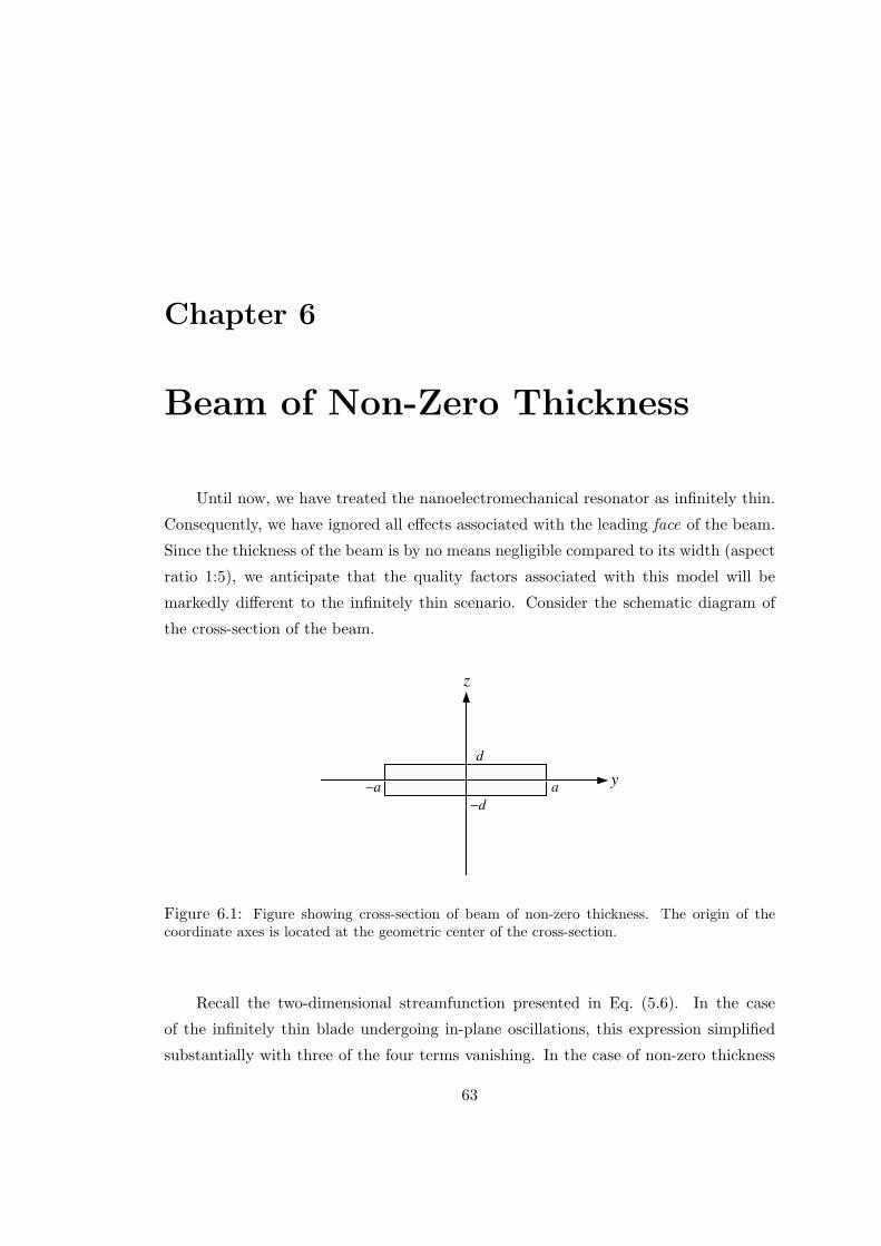
Chapter 6
Beam of Non-Zero Thickness
Until now, we have treated the nanoelectromechanical resonator as infinitely thin.
Consequently, we have ignored all effects associated with the leading face of the beam.
Since the thickness of the beam is by no means negligible compared to its width (aspect
ratio 1:5), we anticipate that the quality factors associated with this model will be
markedly different to the infinitely thin scenario. Consider the schematic diagram of
the cross-section of the beam.
−a ay
z
d
−d
Figure 6.1: Figure showing cross-section of beam of non-zero thickness. The origin of thecoordinate axes is located at the geometric center of the cross-section.
Recall the two-dimensional streamfunction presented in Eq. (5.6). In the case
of the infinitely thin blade undergoing in-plane oscillations, this expression simplified
substantially with three of the four terms vanishing. In the case of non-zero thickness
63

64
however, very little simplification is possible. We have
ψ =∫C
[ψGn − ψnΩ− ωΨn +
1µpΨl
]dl, (6.1)
where the subscripts n and l denote derivatives with respect to the normal and tan-
gential coordinates to the surface respectively. Recall that the contour C is taken to
enclose the entire fluid and so the normal vector points out of the fluid.
6.1 No-Slip Boundary Condition
Let us first apply the no-slip boundary condition traditionally used in continuum
mechanics. As previously discussed, this is not strictly valid given the relatively large
Knudsen number. However, this will serve as a good first approximation and indeed
will allow us to set up the machinery necessary for application of the slip model in the
proceeding section. For two-dimensional flow in the y-z plane, the fluid velocity is given
by
u = ∇× (ψx) =∂ψ
∂zy − ∂ψ
∂yz.
If we demand that the fluid velocity on Cbeam is precisely equal to the velocity of
the beam itself, we see that for unidirectional motion of the beam (Ubeam = Ubeamy),
the following equations must hold at the surface of the beam:
∂ψ
∂z= Ubeam and
∂ψ
∂y= 0. (6.2)
We require the precise form of the streamfunction on Cbeam. Unfortunately, Eq. (6.2)
cannot provide this. We thus proceed by taking a very different approach to that of
the previous chapters. We know that for a stationary beam, the surface constitutes a
single streamline on which the streamfunction is constant. It follows that if we pose the
problem in the reference frame of the oscillating beam, we can resolve the dilemma of
the unknown streamfunction.

Chapter 6. Beam of Non-Zero Thickness 65
Let us consider a stationary beam surrounded by an infinite fluid oscillating in the
y-direction at angular frequency ω. We write the fluid velocity in the following way:
u = ubeam + u,
where ubeam is the velocity of the beam. The corresponding boundary conditions are
given by
u = 0 at beam surface (no-slip condition),
u = −ubeam at infinity.
The linearized Fourier transformed governing equation for the fluid is given by
Eq. (2.3). Substitution of the above form of u yields
−iρω(ubeam + u) = −∇P + µ∇2(ubeam + u).
Noting that ubeam = Ubeamy and ∇2ubeam = 0, we see that
−iρωu = −∇(P − iρωUbeamy
)+ µ∇2u. (6.3)
The governing equation remains unchanged except for the inclusion of an extra
body force term. This is a direct consequence of transforming into the non-inertial
reference frame associated with the oscillating beam. We can proceed with the boundary
integral formulation working in this new reference frame. Since the fluid infinitely far
from the beam is no longer stationary, we must treat the contour integral around C
with caution. Remember that this contour encloses the entire fluid and so we write
C = Cbeam + C∞ as depicted in Fig. 6.2. Strictly speaking C∞ is an infinitely large
contour that encloses the entire system, however we must first treat it as finite and
proceed to take the limit as r →∞.

66
dl
n
(-a,-d)
(-a,d) (a,d)
(a,-d)
(-r1,r2)
fluid
beam
fluid
fluid
(r1,r2)
(r1,-r2)(-r1,-r2)
(a)
C1
C2
C3
C4
dl
n
dl
n
(-r1,r2)
fluid
beam
(r1,r2)
(r1,-r2)(-r1,-r2)
(b)
Figure 6.2: Diagrams of the contour enclosing the entire fluid. We see that C = Cbeam + C∞as depicted in Figure 6.2(b).

Chapter 6. Beam of Non-Zero Thickness 67
Equation (6.1) can be written in terms of the two constituent contours of C:
ψ =∫Cbeam
[ψGn−ψnΩ−ωΨn+
1µpΨl
]dl+
∫C∞
[ψGn−ψnΩ−ωΨn+
1µpΨl
]dl. (6.4)
We note that infinitely far from the beam, the flow is uniform. Thus, both the
vorticity and pressure are zero and the streamfunction can be written as ψ = −Ubeamz.
Furthermore, the streamfunction is constant on Cbeam since the beam is stationary in
the reference frame we are considering. Without loss of generality we can thus take
ψ = ψn = 0 on Cbeam. Equation (6.4) thus becomes
ψ =∫Cbeam
[− ωΨn +
1µpΨl
]dl +
∫C∞
[ψGn − ψnΩ
]dl. (6.5)
The Green’s functions G(y, z; y′, z′) and Ω(y, z; y′, z′) presented earlier are
G =12π
log(αR), (6.6)
Ω = − 12πK0(αR), (6.7)
where R =√
(y − y′)2 + (z − z′)2. Since Ω is exponentially small at infinity, we note
that the corresponding contribution to the integral in Eq. (6.5) vanishes. Furthermore,
we can evaluate the following integral:∫C∞
ψGndl = −Ubeamz′,
where we have made use of the fact that ∇2G = 0 on C∞. The streamfunction for the
fluid can now be written primarily in terms of the unknown quantities ω and p on the
surface of the beam. We find that
ψ(y′, z′) = −Ubeamz′ +
∫Cbeam
[− ωΨn +
1µpΨl
]dl. (6.8)
The integral in the above equation can be interpreted as the perturbation to the
uniform flow streamfunction, attributed to the presence of the beam. In the absence
of the beam, the integral in Eq. (6.8) vanishes and we are left with the streamfunction
corresponding to uniform flow. We consider four distinct components of the contour
Cbeam as depicted in Fig. 6.3.

68
C1
C2
C3
C4
dl
n
Figure 6.3: Contour around the face of the beam. Cbeam = C1 + C2 + C3 + C4.
We consider motion of the beam to be strictly in the y-direction. Since each path
Ci represents a straight line parallel to either the y or z-axes, we can replace the line
integrals with integrals over y and z. For example, on C1 we have dl = dz, ∂/ ∂l = ∂/ ∂z
and ∂/ ∂n = − ∂/ ∂y. Similar expressions follow for the other three faces. We make
use of the fact that for pure in-plane motion, the pressure on the surface of the beam is
symmetric about the y-axis and antisymmetric about the z-axis. Thus, p2(y) = p4(y)
and p1(z) = −p3(z). Conversely, the vorticity at the surface is antisymmetric about
the y-axis and symmetric about the z-axis. Hence, ω2(y) = −ω4(y) and ω1(z) = ω3(z).
With this in mind Eq. (6.8) becomes
ψ(y′, z′) = −Ubeamz′
+∫ d
−d
[ω1(z)
(Ψy
∣∣y=a
−Ψy
∣∣y=−a
)+
1µp1(z)
(Ψz
∣∣y=a
+ Ψz
∣∣y=−a
)]dz
+∫ a
−a
[ω2(y)
(Ψz
∣∣z=d
+ Ψz
∣∣z=−d
)− 1µp2(y)
(Ψy
∣∣z=d
−Ψy
∣∣z=−d
)]dy. (6.9)
We have posed this problem in the reference frame of the beam itself and so the fluid
is considered stationary on Cbeam. Equation (6.2) is thus an inappropriate boundary
condition. Instead we have
∂ψ(y′, z′)∂z′
∣∣∣∣∣beam
= 0 and∂ψ(y′, z′)
∂y′
∣∣∣∣∣beam
= 0. (6.10)
Combining Eqs. (6.9) and (6.10), we obtain the following pair of coupled integral equa-

Chapter 6. Beam of Non-Zero Thickness 69
tions:
Ubeam =∫ d
−d
[ω1(z)
(Ψyz′
∣∣y=a
−Ψyz′∣∣y=−a
)+
1µp1(z)
(Ψzz′
∣∣y=a
+ Ψzz′∣∣y=−a
)]dz
+∫ a
−a
[ω2(y)
(Ψzz′
∣∣z=d
+ Ψzz′∣∣z=−d
)− 1µp2(y)
(Ψyz′
∣∣z=d
−Ψyz′∣∣z=−d
)]dy,
(6.11)
and
0 =∫ d
−d
[ω1(z)
(Ψyy′
∣∣y=a
−Ψyy′∣∣y=−a
)+
1µp1(z)
(Ψzy′
∣∣y=a
+ Ψzy′∣∣y=−a
)]dz
+∫ a
−a
[ω2(y)
(Ψzy′
∣∣z=d
+ Ψzy′∣∣z=−d
)− 1µp2(y)
(Ψyy′
∣∣z=d
−Ψyy′∣∣z=−d
)]dy, (6.12)
where the right hand sides of the above equations are evaluated on the face of the beam.
We now proceed to scale these equations in the following way. Since the dominant length
scale is the width of the beam (y-direction), the spatial variables are scaled according
to
ξ =y
a, χ =
z
a. (6.13)
The pressure and vorticity are scaled as
P1(χ) =a
µUbeamp1(z), Λ1(χ) =
a
Ubeamω1(z),
P2(ξ) =a
µUbeamp2(y), Λ2(ξ) =
a
Ubeamω2(y). (6.14)
The beam for which we possess experimental data has an aspect ratioA = widththickness =
2a2d = 5, however we continue the formulation of this model in terms of an arbitrary as-
pect ratio A. This will enable us to check the model against the infinitely thin results
obtained in Chapter 5 by setting A→∞. From this scaling, it follows that ξ ∈ [−1, 1]
and χ ∈ [−1/A, 1/A]. Adopting the scaled Green’s function presented in Eq. (5.34), the
integral equations in (6.11) and (6.12) can be written as
70
1 =∫ 1/A
−1/A
[Λ1(χ)
(Ψξχ′
∣∣ξ=1
− Ψξχ′∣∣ξ=−1
)+ P1(χ)
(Ψχχ′
∣∣ξ=1
+ Ψχχ′∣∣ξ=−1
)]dχ
+∫ 1
−1
[Λ2(ξ)
(Ψχχ′
∣∣χ=1/A
+ Ψχχ′∣∣χ=−1/A
)+ P2(ξ)
(Ψξχ′
∣∣χ=−1/A
− Ψξχ′∣∣χ=1/A
)]dξ,
(6.15)
0 =∫ 1/A
−1/A
[Λ1(χ)
(Ψξξ′
∣∣ξ=1
− Ψξξ′∣∣ξ=−1
)+ P1(χ)
(Ψχξ′
∣∣ξ=1
+ Ψχξ′∣∣ξ=−1
)]dχ
+∫ 1
−1
[Λ2(ξ)
(Ψχξ′
∣∣χ=1/A
+ Ψχξ′∣∣χ=−1/A
)+ P2(ξ)
(Ψξξ′
∣∣χ=−1/A
− Ψξξ′∣∣χ=1/A
)]dξ.
(6.16)
Notice that in the limit when A → ∞, Eq. (6.15) collapses to become equivalent
to Eq. (5.18), the only exception being that in Chapter 5 we considered the vorticity
jump rather than the actual vorticity. Henceforth, we will drop the ‘bar’ notation for
Ψ and consider it to be scaled.
6.1.1 Numerical Solution Method
We now implement a similar numerical method to that used in Chapter 5 in order
to solve the above integral equations. This is significantly harder than for the beam of
zero thickness since we now have two coupled equations. We must transform the integral
equations into a system of matrix equations using an appropriate quadrature method. In
discretizing the integrals over the faces of the beam, we adopt the unequal quadrature
points with χm = − 1A cos(πm/M) for m = 0, 1, . . . ,M and ξn = − cos(πn/N) for
n = 0, 1, . . . , N . This will account for the presence of the square-root singularities
in the pressure and vorticity at the corners of the beam cross-section [5]. Provided
we discretize the integration intervals using a sufficiently large number of segments,
the pressure and vorticity can be approximated as constant in each interval. That is,
P1(χ) = P1m and Λ1(χ) = Λ1m for χm < χ < χm+1 and P2(ξ) = P2n and Λ2(ξ) = Λ2n
for ξn < ξ < ξn+1. Equations (6.15) and (6.16) thus become

Chapter 6. Beam of Non-Zero Thickness 71
M−1∑m=0
[Λ1mI1 + P1mI2
]+N−1∑n=0
[Λ2nI3 + P2nI4
]= 1, (6.17)
M−1∑m=0
[Λ1mJ1 + P1mJ2
]+N−1∑n=0
[Λ2nJ3 + P2nJ4
]= 0, (6.18)
where
I1 =∫ χm+1
χm
(Ψξχ′
∣∣ξ=1
−Ψξχ′∣∣ξ=−1
)dχ,
I2 =∫ χm+1
χm
(Ψχχ′
∣∣ξ=1
+ Ψχχ′∣∣ξ=−1
)dχ,
I3 =∫ ξn+1
ξn
(Ψχχ′
∣∣χ=1/A
+ Ψχχ′∣∣χ=−1/A
)dξ,
I4 =∫ ξn+1
ξn
(Ψξχ′
∣∣χ=−1/A
−Ψξχ′∣∣χ=1/A
)dξ,
(6.19)
J1 =∫ χm+1
χm
(Ψξξ′
∣∣ξ=1
−Ψξξ′∣∣ξ=−1
)dχ,
J2 =∫ χm+1
χm
(Ψχξ′
∣∣ξ=1
+ Ψχξ′∣∣ξ=−1
)dχ,
J3 =∫ ξn+1
ξn
(Ψχξ′
∣∣χ=1/A
+ Ψχξ′∣∣χ=−1/A
)dξ,
J4 =∫ ξn+1
ξn
(Ψξξ′
∣∣χ=−1/A
−Ψξξ′∣∣χ=1/A
)dξ.
The above integrals still have both ξ′ and χ′ unspecified. We demand that Eqs. (6.17)
and (6.18) hold at the midpoint of each segment on the discretized intervals. In other
words, we force these equations to hold at (ξ′, χ′) = (ξ′k,1A) = (1
2(ξk + ξk+1), 1A) for
k = 0, . . . , N − 1 and (ξ′, χ′) = (1, χ′j) = (1, 12(χj + χj+1)) for j = 0, . . . ,M − 1.
Applying these conditions to Eq. (6.17) yields the following matrix-vector equation:
[I1(1, χ′j)
]jm
[I2(1, χ′j)
]jm
[I3(1, χ′j)
]jn
[I4(1, χ′j)
]jn[
I1(ξ′k,1A)
]km
[I2(ξ′k,
1A)
]km
[I3(ξ′k,
1A)
]kn
[I4(ξ′k,
1A)
]kn
Λ1
P1
Λ2
P2
=
1
1...
1
.

72
If x is the vector containing the unknowns, then we write this in the following form:
Ax = a. (6.20)
Similarly, Eq. (6.18) becomes
[J1(1, χ′j)
]jm
[J2(1, χ′j)
]jm
[J3(1, χ′j)
]jn
[J4(1, χ′j)
]jn[
J1(ξ′k,1A)
]km
[J2(ξ′k,
1A)
]km
[J3(ξ′k,
1A)
]kn
[J4(ξ′k,
1A)
]kn
Λ1
P1
Λ2
P2
=
0
0...
0
,(6.21)
or alternatively
Bx = b. (6.22)
In the above equations, A and B are matrices of dimension (M +N)× (2M +2N)
while x, a and b are vectors of length 2M+2N . We want to solve Eqs. (6.20) and (6.22)
simultaneously. With the dimensions of these systems in mind, it becomes apparent
that we can construct one large system to be solved,[A
B
]x =
[a
b
],
or
Cx = d. (6.23)
We have now posed the problem in such a way as to have 2M +2N unknowns, and
the same number of corresponding equations. Construction of the matrix C can be ex-
tremely slow if we fail to make several simplifications first. We note that the majority of
the integrals in Eq. (6.19) can be evaluated exactly without resorting to numerical meth-
ods. Noting that Ψξχ′(ξ, χ; ξ′, χ′) = Ψχξ′(ξ, χ; ξ′, χ′), Ψξ′(ξ, χ; ξ′, χ′) = −Ψξ(ξ, χ; ξ′, χ′)
and Gχξ′(ξ, χ; ξ′, χ′) = Gξχ′(ξ, χ; ξ′, χ′), we see that that all but two of the integrals
can be evaluated directly by the Fundamental Theorem of Calculus. The integrals I3and J1 are more stubborn and we must resort to numerical integration. The matrix C
and vector d can be constructed using a software package such as mathematica R© .
Consider Figs. 6.4 and 6.5 on the following pages. These display the computed vorticity
and pressure on faces 1 and 2 of the beam for β = 0.3527 and A = 5.

Chapter 6. Beam of Non-Zero Thickness 73
As anticipated, we see that the vorticity and pressure on C1 are odd and even
functions of χ respectively. Conversely, the vorticity and pressure on C2 are even and
odd functions of ξ respectively. We need not display the computed results for C3 and
C4 since these are trivially found using the symmetry properties that we exploited to
simplify the problem from the outset.

74
Re HL1L
Im HL1L
-0.2 -0.1 0.1 0.2 Χ
-6
-4
-2
2
4
6
L1
(a)
Re HP1L
Im HP1L
-0.2 -0.1 0.1 0.2 Χ
-10
-5
5
10
15
P1
(b)
Figure 6.4: (a) Vorticity and (b) pressure distribution on the leading face of the beam (C1; seeFig. 6.3) for dimensionless frequency β = 0.3527 and aspect ratio A = 5.

Chapter 6. Beam of Non-Zero Thickness 75
Re HL2L
Im HL2L
-1.0 -0.5 0.5 1.0 Ξ
-4
-2
2
4
L2
(a)
Im HP2L
Re HP2L
-1.0 -0.5 0.5 1.0 Ξ
-1.0
-0.5
0.5
1.0
P2
(b)
Figure 6.5: (a) Vorticity and (b) pressure distribution on the top face of the beam (C2; seeFig. 6.3) for dimensionless frequency β = 0.3527 and aspect ratio A = 5.
76
6.1.2 Calculation of Hydrodynamic Function
We now endeavour to calculate the force on the beam as it oscillates. There are
a few subtleties which we must bear in mind when performing this calculation. Recall
that in undertaking this problem, we have considered the non-inertial reference frame
associated with the beam. In the rest frame of the laboratory, we have an additional
body force term which is a direct consequence of this transformation. From Eq. (6.3),
we see that the pressure in the reference frame of the laboratory is given by
p = pcalculated + iρωUbeamy,
where pcalculated is the (unscaled) pressure arising from our preceding numerical analysis.
Noting that Ubeam = −iωW , we see that
p = pcalculated + ρω2yW . (6.24)
The vector force F acting on any three-dimensional body with surface S, moving in any
manner in an incompressible fluid is given by [5]
F =∫S
[− pdS + µω × dS
].
The component of this force in the y−direction is then
Fy = j · F =∫Cbeam
[− pdz + µωdy
].
Since we know the pressure and vorticity on all four faces of the beam, we can readily
evaluate the total force in the y−direction,
F = −∫ d
−d
[2p1(z) + 2ρω2aW
]dz −
∫ a
−a
[2µω2(y)
]dy.
We must take care not to confuse the angular frequency ω with the fluid vortic-
ity ω2(y). Making use of the scaled variables from Eqs. (6.13) and (6.14), the above
expression can be rewritten as follows:
F = 2µiωW[Jpres(β) + Jvort(β)
]− 4ρadω2W , (6.25)

Chapter 6. Beam of Non-Zero Thickness 77
where
Jpres =∫ 1/A
−1/AP1(χ)dχ and Jvort =
∫ 1
−1Λ2(ξ)dξ. (6.26)
Since we have solved the problem in terms of the scaled pressure and vorticity, the
integrals Jpres and Jvort can be readily computed using mathematica R© . Equating
(2.4) and (6.25) yields the following expression for the hydrodynamic function:
Γ(ω) =2iπβ
[Jpres(β) + Jvort(β)
]− 4πA
. (6.27)
It is particularly interesting to see that the contribution to Γ(ω) due to the change
of reference frame depends only on A. Furthermore, 4/(πA) → 0 as A → ∞ and so
there is no additional body force for an infinitely thin blade. In order to evaluate the
hydrodynamic function for a particular value of β, we must construct and solve the
matrix system mentioned earlier numerically and proceed to integrate the calculated
pressure and vorticity over the faces of the beam. From a computational point of view,
this procedure is extremely demanding. Indeed, if we use M = N = 20; a reasonably
modest number of subdivisions on each face, we are required to construct an 80 × 80
matrix, of which 1,600 entries are numerically computed integrals! This process needs
to be undertaken every single time we want to evaluate Γ for some aspect ratio A
and frequency β. One can appreciate that plotting the hydrodynamic function as a
continuous curve is very difficult. Nevertheless, it is possible to evaluate Γ at sufficiently
many points to enable us to construct an accurate representation of the behaviour of
Γ over the appropriate frequency domain. As an aside, we note that production of
the following results in Fig. 6.6 required approximately 10 hours of CPU time using a
3.2GHz Pentium 4 processor.

78
10−1
100
10110
−1
100
101
102
β
Γ
Figure 6.6: Real (solid) and imaginary (dotted) components of the hydrodynamic function asa function of dimensionless frequency β. The above results correspond to aspect ratio A = 5and have been computed using M = N = 30 subdivisions for small β and M = N = 40 forlarger values of β. This value of A was chosen since it coincides exactly with the dimensions ofthe beams used by Bargatin et al. [2].

Chapter 6. Beam of Non-Zero Thickness 79
6.1.3 Alternative Scaling For Out-of-Plane Modes
So far we have been primarily concerned with in-plane motion of the beam. This
corresponds to motion in the y-direction for A > 1. The hydrodynamic function for
out-of-plane motion of an infinitely thin beam is known [3]. We would ultimately like to
check our model in this particular limiting case. The situation of out-of-plane motion
can be adopted be setting A < 1. Care must be taken when choosing such values of A.
Recall that the dimensionless frequency, spatial dimensions, vorticity and pressure have
all been scaled according to the dominant length scale. For in-plane motion (A > 1),
the characteristic length scale is the width of the beam, and so we chose to scale using
a. Conversely, for A < 1 the thickness of the beam becomes the characteristic length
scale and so it becomes appropriate to scale the aforementioned quantities in terms of
d. This is particularly easy to do. We see that the spatial discretization of the beam
faces is done with χm = − cos(πm/M) for m = 0, 1, . . . ,M and ξn = −A cos(πn/N) for
n = 0, 1, . . . , N . It turns out that the expression for the hydrodynamic function is very
similar to Eq. (6.27) and is given by
Γout(ω) =2iπβ
[Jpres(β) + Jvort(β)
]− 4A
π. (6.28)
Notice that 4A/π → 0 as A→ 0. That is, the body force contribution arising from
solving the problem in a non-inertial reference frame vanishes for an infinitely thin blade.
This is perhaps slightly counter-intuitive since one would expect that for out-of-plane
motion, there would be a body force. The consequences of changing reference frame de-
pend on the volume of fluid displaced by the beam and not on the exposed surface area.
It is now possible to check the hydrodynamic function calculated by the present
model against the values obtained by Sader [3] simply by choosing A→ 0. Furthermore,
the present model should yield the same results as obtained in Chapter 5 in the case
as A → ∞ since this scenario represents in-plane motion of an infinitely thin blade.
Consider Fig. 6.7, which shows the computed hydrodynamic function as a function
of aspect ratio A. The dotted lines represent the infinitely thin solutions previously
mentioned. One can see that there is very good agreement between the present model
and the two aforementioned limiting cases.
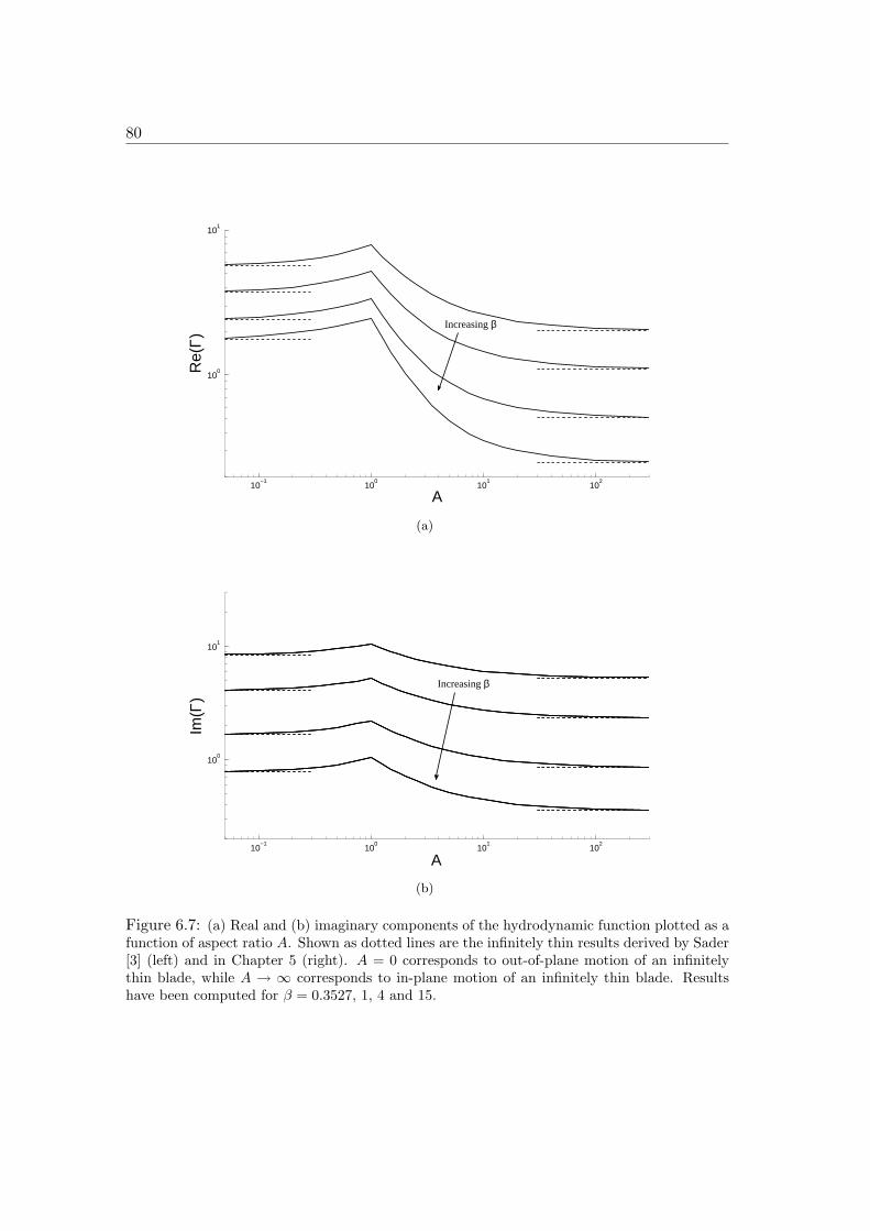
80
10−1
100
101
102
100
101
A
Re(
Γ)
Increasing β
(a)
10−1
100
101
102
100
101
A
Im(Γ
)
Increasing β
(b)
Figure 6.7: (a) Real and (b) imaginary components of the hydrodynamic function plotted as afunction of aspect ratio A. Shown as dotted lines are the infinitely thin results derived by Sader[3] (left) and in Chapter 5 (right). A = 0 corresponds to out-of-plane motion of an infinitelythin blade, while A → ∞ corresponds to in-plane motion of an infinitely thin blade. Resultshave been computed for β = 0.3527, 1, 4 and 15.

Chapter 6. Beam of Non-Zero Thickness 81
One may wonder why there exists a sharp peak at A = 1 in Fig. 6.7. We must bear
in mind that in constructing these plots, we are really amalgamating two different aspect
ratio regimes corresponding to the respective scalings for the in-plane and out-of-plane
oscillations. Thus, we can actually think of this “peak” as the point where the length
scale of the problem switches. It is important to note that starting from A = 1, as A→ 0
and A → ∞ , both the real and imaginary components of the hydrodynamic function
are monotonic decreasing. That is, for a particular scaling, Γ decreases monotonically
as the blade becomes thinner. This is in perfect accordance with our physical intuition.
Recall that the real and imaginary components of the hydrodynamic function represent
the added mass and viscous losses respectively of the beam as it vibrates. We expect
that these would decrease as the blade thickness decreases and this is indeed what is
observed.

82
6.2 First-Order Slip Boundary Condition
We now seek to apply the slip boundary condition at the surface of the beam. As
discussed in preceding chapters, it is necessary to consider a boundary condition of this
form since the mean free path of air molecules is comparable to the thickness of the
blades used by Bargatin et al. [2]. Indeed, at this scale (Kn ≈ 0.17), the no-slip bound-
ary condition traditionally used in continuum mechanics is certainly not applicable.
We will see that the subsequent correction to the no-slip results is extremely strong,
and as such, seeking anything more than a first-order correction is unreasonable. The
cross-section of the beam is still given as in Fig. 6.1, the only thing changing in our
analysis being the boundary condition at the beam surface.
Recall that in Section 6.1 we posed the problem in terms of a stationary beam
surrounded by a fluid oscillating at infinity so that the streamfunction could be set to
zero at the beam surface. This analysis follows in exactly the same way, except that in
moving from Eq. (6.4) to Eq. (6.5), we can no longer set ψn = 0. Differentiation of the
streamfunction with respect to the normal coordinate yields the tangential velocity at
the beam surface which is certainly no longer zero! Instead we obtain
ψ =∫Cbeam
[− ψnΩ− ωΨn +
1µpΨl
]dl +
∫C∞
[ψGn − ψnΩ
]dl, (6.29)
where G and Ω are the Green’s function defined in Eqs. (6.6) and (6.7). Since the
pressure and vorticity infinitely far from the beam will be unaffected by the presence
of slip, this equation reduces to give
ψ(y′, z′) = −Ubeamz′ +
∫Cbeam
[− ψnΩ− ωΨn +
1µpΨl
]dl. (6.30)
This is precisely the same as in Eq. (6.8) with the addition of one extra term. We can
actually write the above equation as
ψ(y′, z′) = ψno-slip(y′, z′)−∫Cbeam
[ψnΩ
]dl, (6.31)
where ψno-slip is given by Eq. (6.8). In order to remove the dependence of Eq. (6.31) on

Chapter 6. Beam of Non-Zero Thickness 83
ψn, we examine the first-order slip boundary condition. This is given by
U∣∣wall
− uw = −γη ∂U∂n
∣∣∣∣wall
, (6.32)
where the subscript n denotes differentiation in the direction of the normal vector,
which points out of the fluid. We again consider the four faces of the beam as distinct
components of the contour Cbeam as in Fig. 6.3. Since the fluid velocity and vorticity
can be written as u = ∇×(ψx) and ω = −∇2ψ respectively, the slip boundary condition
becomes
ψz′ = 0 on C1 (no penetration condition),
ψz′ + γηω2 = 0 on C2 (slip condition), (6.33)
ψy′ + γηω1 = 0 on C1 (slip condition),
ψy′ = 0 on C2 (no penetration condition),
and we have∫Cbeam
(ψnΩ
)dl = γη
[ ∫ d
−dω1(z)
(Ω
∣∣y=a
+Ω∣∣y=−a
)dz+
∫ a
−aω2(y)
(Ω
∣∣z=d−Ω
∣∣z=−d
)dy
].
Combining this with Eq. (6.9), we see that the streamfunction can be written as
ψ(y′, z′) = −Ubeamz′
+∫ d
−d
[ω1(z)
(Ψy
∣∣y=a
−Ψy
∣∣y=−a
)+
1µp1(z)
(Ψz
∣∣y=a
+ Ψz
∣∣y=−a
)]dz
+∫ a
−a
[ω2(y)
(Ψz
∣∣z=d
+ Ψz
∣∣z=−d
)− 1µp2(y)
(Ψy
∣∣z=d
−Ψy
∣∣z=−d
)]dy
− γη
[ ∫ d
−dω1(z)
(Ω
∣∣y=a
+ Ω∣∣y=−a
)dz +
∫ a
−aω2(y)
(Ω
∣∣z=d
− Ω∣∣z=−d
)dy
].
(6.34)

84
Regrouping the terms slightly yields
ψ(y′, z′) = −Ubeamz′
+∫ d
−d
[ω1(z)
(Ψy
∣∣y=a
−Ψy
∣∣y=−a − γη(Ω
∣∣y=a
+ Ω∣∣y=−a)
)+
1µp1(z)
(Ψz
∣∣y=a
+ Ψz
∣∣y=−a
)]dz
+∫ a
−a
[ω2(y)
(Ψz
∣∣z=d
+ Ψz
∣∣z=−d − γη(Ω
∣∣z=d
− Ω∣∣z=−d)
)− 1µp2(y)
(Ψy
∣∣z=d
−Ψy
∣∣z=−d
)]dy.
(6.35)
The incorporation of slip has altered the streamfunction slightly by introduction of
additional terms. If we force Eq. (6.35) to satisfy the boundary conditions in Eq. (6.33)
we obtain the following four equations:
Ubeam =∫ d
−d
[ω1(z)
(Ψyz′
∣∣y=a
−Ψyz′∣∣y=−a − γη(Ωz′
∣∣y=a
+ Ωz′∣∣y=−a)
)+
1µp1(z)
(Ψzz′
∣∣y=a
+ Ψzz′∣∣y=−a
)]dz
+∫ a
−a
[ω2(y)
(Ψzz′
∣∣z=d
+ Ψzz′∣∣z=−d − γη(Ωz′
∣∣z=d
− Ωz′∣∣z=−d)
)− 1µp2(y)
(Ψyz′
∣∣z=d
−Ψyz′∣∣z=−d
)]dy on C1,
(6.36)
Ubeam =∫ d
−d
[ω1(z)
(Ψyz′
∣∣y=a
−Ψyz′∣∣y=−a − γη(Ωz′
∣∣y=a
+ Ωz′∣∣y=−a)
)+
1µp1(z)
(Ψzz′
∣∣y=a
+ Ψzz′∣∣y=−a
)]dz
+∫ a
−a
[ω2(y)
(Ψzz′
∣∣z=d
+ Ψzz′∣∣z=−d − γη(Ωz′
∣∣z=d
− Ωz′∣∣z=−d)
)− 1µp2(y)
(Ψyz′
∣∣z=d
−Ψyz′∣∣z=−d
)]dy + γηω2(y′) on C2,
(6.37)
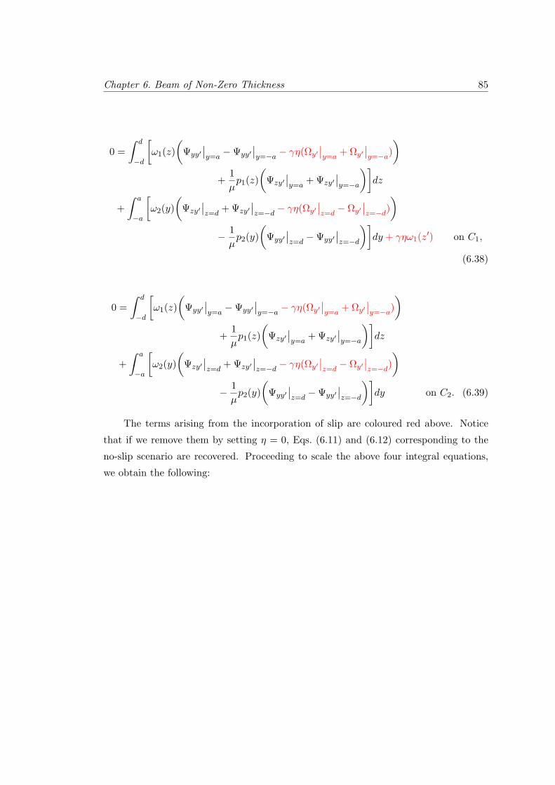
Chapter 6. Beam of Non-Zero Thickness 85
0 =∫ d
−d
[ω1(z)
(Ψyy′
∣∣y=a
−Ψyy′∣∣y=−a − γη(Ωy′
∣∣y=a
+ Ωy′∣∣y=−a)
)+
1µp1(z)
(Ψzy′
∣∣y=a
+ Ψzy′∣∣y=−a
)]dz
+∫ a
−a
[ω2(y)
(Ψzy′
∣∣z=d
+ Ψzy′∣∣z=−d − γη(Ωy′
∣∣z=d
− Ωy′∣∣z=−d)
)− 1µp2(y)
(Ψyy′
∣∣z=d
−Ψyy′∣∣z=−d
)]dy + γηω1(z′) on C1,
(6.38)
0 =∫ d
−d
[ω1(z)
(Ψyy′
∣∣y=a
−Ψyy′∣∣y=−a − γη(Ωy′
∣∣y=a
+ Ωy′∣∣y=−a)
)+
1µp1(z)
(Ψzy′
∣∣y=a
+ Ψzy′∣∣y=−a
)]dz
+∫ a
−a
[ω2(y)
(Ψzy′
∣∣z=d
+ Ψzy′∣∣z=−d − γη(Ωy′
∣∣z=d
− Ωy′∣∣z=−d)
)− 1µp2(y)
(Ψyy′
∣∣z=d
−Ψyy′∣∣z=−d
)]dy on C2. (6.39)
The terms arising from the incorporation of slip are coloured red above. Notice
that if we remove them by setting η = 0, Eqs. (6.11) and (6.12) corresponding to the
no-slip scenario are recovered. Proceeding to scale the above four integral equations,
we obtain the following:

86
1 =∫ 1/A
−1/A
[Λ1(χ)
(Ψξχ′
∣∣ξ=1
− Ψξχ′∣∣ξ=−1
− γη(Ωχ′∣∣ξ=1
+ Ωχ′∣∣ξ=−1
))
+ P1(χ)(
Ψχχ′∣∣ξ=1
+ Ψχχ′∣∣ξ=−1
)]dχ
+∫ 1
−1
[Λ2(ξ)
(Ψχχ′
∣∣χ=1/A
+ Ψχχ′∣∣χ=−1/A
− γη(Ωχ′∣∣χ=1/A
− Ωχ′∣∣χ=−1/A
))
+ P2(ξ)(
Ψξχ′∣∣χ=−1/A
− Ψξχ′∣∣χ=1/A
)]dξ on C1, (6.40)
1 =∫ 1/A
−1/A
[Λ1(χ)
(Ψξχ′
∣∣ξ=1
− Ψξχ′∣∣ξ=−1
− γη(Ωχ′∣∣ξ=1
+ Ωχ′∣∣ξ=−1
))
+ P1(χ)(
Ψχχ′∣∣ξ=1
+ Ψχχ′∣∣ξ=−1
)]dχ
+∫ 1
−1
[Λ2(ξ)
(Ψχχ′
∣∣χ=1/A
+ Ψχχ′∣∣χ=−1/A
− γη(Ωχ′∣∣χ=1/A
− Ωχ′∣∣χ=−1/A
))
+ P2(ξ)(
Ψξχ′∣∣χ=−1/A
− Ψξχ′∣∣χ=1/A
)]dξ + γηΛ2(ξ′) on C2,
(6.41)
0 =∫ 1/A
−1/A
[Λ1(χ)
(Ψξξ′
∣∣ξ=1
− Ψξξ′∣∣ξ=−1
− γη(Ωξ′∣∣ξ=1
+ Ωξ′∣∣ξ=−1
))
+ P1(χ)(
Ψχξ′∣∣ξ=1
+ Ψχξ′∣∣ξ=−1
)]dχ
+∫ 1
−1
[Λ2(ξ)
(Ψχξ′
∣∣χ=1/A
+ Ψχξ′∣∣χ=−1/A
− γη(Ωξ′∣∣χ=1/A
− Ωξ′∣∣χ=−1/A
))
+ P2(ξ)(
Ψξξ′∣∣χ=−1/A
− Ψξξ′∣∣χ=1/A
)]dξ + γηΛ1(χ′) on C1, (6.42)
0 =∫ 1/A
−1/A
[Λ1(χ)
(Ψξξ′
∣∣ξ=1
− Ψξξ′∣∣ξ=−1
− γη(Ωξ′∣∣ξ=1
+ Ωξ′∣∣ξ=−1
))
+ P1(χ)(
Ψχξ′∣∣ξ=1
+ Ψχξ′∣∣ξ=−1
)]dχ
+∫ 1
−1
[Λ2(ξ)
(Ψχξ′
∣∣χ=1/A
+ Ψχξ′∣∣χ=−1/A
− γη(Ωξ′∣∣χ=1/A
− Ωξ′∣∣χ=−1/A
))
+ P2(ξ)(
Ψξξ′∣∣χ=−1/A
− Ψξξ′∣∣χ=1/A
)]dξ on C2. (6.43)

Chapter 6. Beam of Non-Zero Thickness 87
6.2.1 Numerical Solution Method
In order to solve the integral equations (6.40) - (6.43), we will use precisely the
same numerical solution method as in Section 6.1. We discretize the integration inter-
vals using Chebyshev points and proceed to construct a giant matrix-vector equation.
Following the same procedure as before, we see that Eqs. (6.40) - (6.43) become
M−1∑m=0
[Λ1mI1 + P1mI2
]+N−1∑n=0
[Λ2nI3 + P2nI4
]= 1 on C1, (6.44)
M−1∑m=0
[Λ1mI1 + P1mI2
]+N−1∑n=0
[Λ2nI3 + P2nI4
]+ γηΛ2(ξ′) = 1 on C2, (6.45)
M−1∑m=0
[Λ1mJ1 + P1mJ2
]+N−1∑n=0
[Λ2nJ3 + P2nJ4
]+ γηΛ1(χ′) = 0 on C1, (6.46)
M−1∑m=0
[Λ1mJ1 + P1mJ2
]+N−1∑n=0
[Λ2nJ3 + P2nJ4
]= 0 on C2, (6.47)
where
I1 =∫ χm+1
χm
(Ψξχ′
∣∣ξ=1
−Ψξχ′∣∣ξ=−1
− γη(Ωχ′∣∣ξ=1
+ Ωχ′∣∣ξ=−1
))dχ,
I2 =∫ χm+1
χm
(Ψχχ′
∣∣ξ=1
+ Ψχχ′∣∣ξ=−1
)dχ,
I3 =∫ ξn+1
ξn
(Ψχχ′
∣∣χ=1/A
+ Ψχχ′∣∣χ=−1/A
− γη(Ωχ′∣∣χ=1/A
− Ωχ′∣∣χ=−1/A
))dξ,
I4 =∫ ξn+1
ξn
(Ψξχ′
∣∣χ=−1/A
−Ψξχ′∣∣χ=1/A
)dξ,
(6.48)
J1 =∫ χm+1
χm
(Ψξξ′
∣∣ξ=1
−Ψξξ′∣∣ξ=−1
− γη(Ωξ′∣∣ξ=1
+ Ωξ′∣∣ξ=−1
))dχ,
J2 =∫ χm+1
χm
(Ψχξ′
∣∣ξ=1
+ Ψχξ′∣∣ξ=−1
)dχ,
J3 =∫ ξn+1
ξn
(Ψχξ′
∣∣χ=1/A
+ Ψχξ′∣∣χ=−1/A
− γη(Ωξ′∣∣χ=1/A
− Ωξ′∣∣χ=−1/A
))dξ,
J4 =∫ ξn+1
ξn
(Ψξξ′
∣∣χ=−1/A
−Ψξξ′∣∣χ=1/A
)dξ.

88
Using the above equations, we can assemble the matrix-vector system. Only a few
small modifications need be made to the mathematica R© code corresponding to the
no-slip case. In addition, we note that half of the integrals involving Ωχ′ and Ωξ′ are
directly integrable whilst for the other half we must resort to numerical integration.
The matrix-vector equation can be written in the following way:
Mx = r,
where x is the global vector containing all of the unknown values of Λ1, P1, Λ2 and P2.
By observation of Eqs. (6.44)-(6.48), it is evident that the matrix-vector equation can
also be written as (M0 + KnM1
)x = r, (6.49)
where the matrices M0 and M1 are independent of Kn = η/b. The vast majority of
computational time is spent constructing M0 and M1. We need only compute these
once for given β and A since solutions corresponding to all Kn can then be quickly
evaluated using the above equation.
We now examine one set of solutions. The plots in Figs. 6.8 and 6.9 show the real
and imaginary components of the vorticity and pressure on the front (C1) and top (C2)
faces of the beam. Although the Knudsen number corresponding to the experiments
undertaken by Bargatin et al. [2] is Kn = η/b = η/2 ≈ 0.17, the results presented are
for Kn = 0.01. We will deal with Kn rather than η from now on since it is more widely
used in the literature. Note that these two quantities differ by a factor of 1/2.
Notice from Figs. 6.8 and 6.9 that the incorporation of slip has the effect of removing
the square-root singularities in the vorticity near the corners. This phenomenon was
observed upon introduction of slip for the infinitely thin blade (see Fig. 5.4). Notice
also that the square-root singularities in the pressure remain intact. Although the
vorticity and pressure are coupled through the global matrix-vector system, we note
that incorporating first-order slip affects elements of the matrix corresponding to the
vorticity only.

Chapter 6. Beam of Non-Zero Thickness 89
Re HL1L
Im HL1L
-0.2 -0.1 0.1 0.2Χ
-2
-1
1
2
L1
(a)
Re HP1L
Im HP1L
-0.2 -0.1 0.1 0.2Χ
-15
-10
-5
5
10
15
P1
(b)
Figure 6.8: (a) Vorticity and (b) pressure distribution on the leading face of the beam (C1;see Fig. 6.3) for dimensionless frequency β = 0.3527, aspect ratio A = 5 and Knudsen numberKn = 0.01.

90
Re HL2L
Im HL2L
-1.0 -0.5 0.5 1.0Ξ
-1.0
-0.5
0.5
1.0
1.5
L2
(a)
Im HP2L
Re HP2L
-1.0 -0.5 0.5 1.0Ξ
-1.0
-0.5
0.5
1.0
P2
(b)
Figure 6.9: (a) Vorticity and (b) pressure distribution on the top face of the beam (C2; seeFig. 6.3) for dimensionless frequency β = 0.3527, aspect ratio A = 5 and Knudsen numberKn = 0.01.

Chapter 6. Beam of Non-Zero Thickness 91
6.2.2 Calculation of Hydrodynamic Function
Once the vorticity and pressure are known on each face of the beam, the sub-
sequent calculation of the hydrodynamic function is relatively straightforward. Recall
Eqs. (6.27) and (6.28) which are expressions for the hydrodynamic function correspond-
ing to in-plane and out-of-plane modes respectively. We note that as well as being de-
pendent on ω (or equivalently β) and A, Γ will also have a dependence on the Knudsen
number Kn = η/b = η/2. As such, we write
Γin(ω,Kn) =2iπβ
[Jpres(β) + Jvort(β)
]− 4πA
for A > 1, (6.50)
Γout(ω,Kn) =2iπβ
[Jpres(β) + Jvort(β)
]− 4A
πfor A < 1. (6.51)
Recall that the above terms involving A arise due to the fact that we have solved
the problem in the non-inertial reference frame of the beam itself. At this stage we
must exercise caution in evaluating the solution as there are several subtleties which, if
ignored, will be catastrophic to our results. In the limit as Kn → ∞, we require that
the hydrodynamic loading on the beam approach zero, since this represents a vacuum.
Consider the following plots which show the computed hydrodynamic function for a
range of Knudsen numbers.
10-5 0.001 0.1 10 1000
2.6
2.8
3.
3.2
3.4
Kn
ReHGL
(a)
10-5 0.001 0.1 10 10006.
6.2
6.4
6.6
6.8
7.
Kn
ImHGL
(b)
Figure 6.10: Figure showing real and imaginary components of the calculated hydrodynamicfunction for β = 0.3527 and A = 5. These correspond to the raw solutions obtained from thematrix-vector equation.
92
Linear Regression of Hydrodynamic Function
The real and imaginary components of the hydrodynamic function level-off as Kn
increases, and fail to approach zero. Upon first glance this is quite concerning, since
it means that we cannot evaluate Γ directly for Kn = 0.17. As Kn → ∞, inspection
of the first-order slip condition yields ∂U/ ∂z → 0. In this limit, the variation in
the velocity diminishes and the pressure contribution on the front face of the beam
prevents the loading from approaching zero. Whilst the numerical process employed
fails to converge to the required solution as Kn increases, we note that Γ is monotonic
decreasing in Kn as required. We remedy the problem by considering very small values
of Kn so as to identify the linear region of the plots in Fig. 6.10. Remember that we
have applied the first-order slip condition and as such will be looking for a correction
to Γ to first-order in Kn. That is, we seek a solution of the following form:
Γ(ω,Kn) = Γ0 + KnΓ1 for Kn 1. (6.52)
We note that the above equation is valid only for small Kn and that Γ0 = Γno-slip
which was found in the preceding section. We proceed to perform a linear regression
for small values of Knudsen number. Consider the following plots, which are the same
curves as in Fig. 6.10, but have been plotted for small Kn only. In order to identify
the linear component of the curve, we consider Kn ∼ 10−7 − 10−6. For larger values
of Kn, the linearity exhibited by the curves in Fig. 6.11 is disrupted. We perform an
interpolation of the points depicted in Fig. 6.11 to degree two, and subsequently extract
the linear component. This is more accurate than simply undertaking a linear regression
since we allow for the curve to be ever so slightly non-linear and correctly capture this
behaviour. We force the interpolated function to go through the point corresponding
to Kn = 0 since this represents the no-slip solution which is well-known and can be
computed to high accuracy. In performing the calculations using mathematica R© , we
have set the working precision to 20 significant figures. We can thus be confident in
the accuracy of the following plots despite the fact that Kn is extremely small. For
the purposes of plotting, we have subtracted the constant Γ0 from the hydrodynamic
function.

Chapter 6. Beam of Non-Zero Thickness 93
æ
æ
æ
æ
æ
æ
æ
æ
æ
æ
æ
0 2.´10-7 4.´10-7 6.´10-7 8.´10-7 1.´10-6
-0.000015
-0.00001
-5.´10-6
0
Kn
Re@G - G0D
(a)
æ
æ
æ
æ
æ
æ
æ
æ
æ
æ
æ
0 2.´10-7 4.´10-7 6.´10-7 8.´10-7 1.´10-6
-0.000014
-0.000012
-0.00001
-8.´10-6
-6.´10-6
-4.´10-6
-2.´10-6
0
Kn
Im@G - G0D
(b)
Figure 6.11: Figure showing real and imaginary components of the hydrodynamic function forβ = 0.3527 and A = 5.

94
Improving Accuracy of Γ for Kn 1
The expression in Eq. (6.52) is linear and monotonic decreasing in Kn. We know
that it is valid for Kn 1, but for sufficiently large Knudsen number, it gives both
Re(Γ) < 0 and Im(Γ) < 0. This is unphysical since it represents a situation where
viscous losses are negative! We seek to improve the convergence of the asymptotic
expansion of the hydrodynamic function in the large Kn regime. Moreover, we require
that Γ → 0 as Kn → ∞. This is done using a Pade approximant and is outlined by
Hinch [12]. We write
Γ = Γ0 + KnΓ1
= Γ0
(1 +
Γ1
Γ0Kn
),
and since 1 + x ≈ (1− x)−1 for small x,
ΓPade(ω,Kn) = Γ0
(1− Γ1
Γ0Kn
)−1
. (6.53)
The expression in Eq. (6.53) has the beauty of being valid in both the low and
high Knudsen number regimes. Thus, the curves in Fig. 6.11 will remain intact. The
Pade approximant approaches zero as Kn → ∞ as it should. In fact, for Kn 1,
ΓPade(ω,Kn) ∼ −Γ20/(Γ1Kn).
GPadeG0+ G1Kn
0.0 0.2 0.4 0.6 0.8 1.00
2
4
6
8
Kn
ReHGL
(a)
GPade
G0+ G1Kn
0 1 2 3 40
5
10
15
20
Kn
ImHGL
(b)
Figure 6.12: Figure showing the real and imaginary components of both the linear constructand the Pade approximant.

Chapter 6. Beam of Non-Zero Thickness 95
Convergence
As with any numerical procedure, understanding the convergence of the computed
solutions is paramount. We now examine the behaviour of the solutions obtained as we
vary the number of subdivisions used in the discretization of the beam faces. We have
already seen how to calculate Γ0 and Γ1 given frequency β and aspect ratio A. Consider
the plots in Fig. 6.13 which show how both the real and imaginary components of Γ0
and Γ1 converge as M and N are increased. For simplicity we have taken M = N in
each case. Values of β = 0.3527 and A = 5 have been adopted for this example.
æ
æ
æ
0 10 20 30 40 50 60
3.145
3.146
3.147
3.148
3.149
3.150
3.151
N
Re@G0D
(a)
æ
æ
æ
0 10 20 30 40 50 606.702
6.703
6.704
6.705
6.706
6.707
N
Im@G0D
(b)
æ
æ
æ
æ
0 10 20 30 40 50 60-17
-16
-15
-14
-13
-12
N
Re@G1D
(c)
æ
æ
æ
æ
0 10 20 30 40 50 60-16
-15
-14
-13
-12
-11
N
Im@G1D
(d)
Figure 6.13: Real and imaginary components of the no-slip hydrodynamic function Γ0 as wellas the first-order correction Γ1 . The solid curve represents the interpolated solution whilst thedotted lines depict the limiting values obtained using Richardson extrapolation.

96
The interpolated functions given by the solid curves in Fig. 6.13 are of the form
a + b/N c and adopt the exponents c = 2 and c = 1/2 for Γ0 and Γ1 respectively.
The values of Γ0 converge fast enough that we can directly evaluate the solution by
taking a sufficiently large value of N . In contrast, the first-order correction converges
much slower, and as such, we are required to extrapolate in order to find the N → ∞solution. We know the exponents of the dominant error terms associated with both
Γ0 and Γ1 respectively. The process of Richardson extrapolation can thus be employed
to accurately predict Γ0 and Γ1 for N → ∞. We emphasise that in order to use this
process, we need to use a series of meshes in which the number of points doubles each
time. For example, we consider N = 5, 10, 20, 40, 80. The problem of slow convergence
of the first-order correction has been remedied by calculating the solution for several
modest values of N , and extrapolating to find the limiting value. We can adopt this
method for any values of β and A.
6.2.3 Comparison with Free Molecular Solution
The solution presented in Eq. (6.53) possesses the correct asymptotic behaviour
for Kn 1 since the solution is constructed using points in this range. We know that
ΓPade(ω,Kn) ≈ −Γ20/(Γ1Kn) → 0 as Kn → ∞. That is, the hydrodynamic function
Γ ∼ Kn−1 as Kn → ∞. We know that this solution exhibits the correct qualitative
behaviour in converging to zero, but cannot be sure that its asymptotic form is indeed
correct. As such, we examine the free molecular solution which we know to be true in
the limit as Kn →∞.
Consider the stationary beam surrounded by a fluid, infinite in extent, and oscil-
lating back and forth with velocity −Ubeam = iωW . The force per unit length exerted
on the beam is given by [10]
F = −µUbeam
Kn
[(1− ε) +
[2 +
π
2
√T +
(2− π
2
√T
)ε
]1A
]. (6.54)
In the above expression, the ratio between the temperature of the beam and the
temperature at infinity is given by T = Tbeam/T∞. The value of ε relates to the extent
of interactions which are specular in nature. Scenarios involving purely diffuse and
specular reflection are represented by ε = 0 and ε = 1 respectively. For simplicity
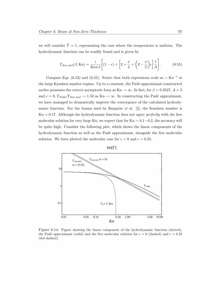
Chapter 6. Beam of Non-Zero Thickness 97
we will consider T = 1, representing the case where the temperature is uniform. The
hydrodynamic function can be readily found and is given by
Γfree mol(β,Kn) =i
Knπβ
[(1− ε) +
[2 +
π
2+
(2− π
2
)ε
]1A
]. (6.55)
Compare Eqs. (6.53) and (6.55). Notice that both expressions scale as ∼ Kn−1 in
the large Knudsen number regime. Up to a constant, the Pade approximant constructed
earlier possesses the correct asymptotic form as Kn →∞. In fact, for β = 0.3527, A = 5
and ε = 0, ΓPade/Γfree mol → 1.53 as Kn →∞. In constructing the Pade approximant,
we have managed to dramatically improve the convergence of the calculated hydrody-
namic function. For the beams used by Bargatin et al. [2], the Knudsen number is
Kn = 0.17. Although the hydrodynamic function does not agree perfectly with the free
molecular solution for very large Kn, we expect that for Kn ∼ 0.1−0.2, the accuracy will
be quite high. Consider the following plot, which shows the linear components of the
hydrodynamic function as well as the Pade approximant, alongside the free molecular
solution. We have plotted the molecular case for ε = 0 and ε = 0.25.
G0+ G1Kn
GPade
Gfree mol HΕ = 0LGfree mol
HΕ = 0.25L
1.000.50 5.000.10 10.000.050.01
0.1
1
10
Kn
Im@GD
Figure 6.14: Figure showing the linear component of the hydrodynamic function (dotted),the Pade approximant (solid) and the free molecular solution for ε = 0 (dashed) and ε = 0.25(dot-dashed).

98
6.3 Progressive Comparison With Experiment
We are now in a position to compare the results predicted by the non-zero thickness
models with experimental values. The principal method of doing so is to evaluate and
compare the quality factors associated with the various in-plane modes. The hydrody-
namic function associated with such modes are given by Eqs. (6.27) and (6.53) for the
cases involving no-slip and slip respectively. These have already been computed, and
so we can readily calculate the associated quality factors using Eq. (2.6). The following
table contains the experimental quality factors, as well as the values predicted by both
the no-slip and first-order slip models. The first five rows correspond to the first five in-
plane modes of the 16µm-long device. The last two rows correspond to the second and
third in-plane resonances of the 24µm-long device. As you can see, there is very good
agreement between the experimentally determined quality factors and those predicted
by the full theoretical model including slip.
Experiment Theoryβ Qfluid only Qfirst-order slip Qno-slip
0.3527 136 144 1010.9223 339 313 2061.7477 535 516 3242.8268 804 749 4504.1315 1160 1002 5790.4346 157 171 1190.8115 311 283 188
Table 6.1: Predicted and experimental quality factors associated with the beam of non-zerothickness

Chapter 6. Beam of Non-Zero Thickness 99
6.4 Determination of Surface Properties
In making the predictions displayed in Table 6.1, we have implicitly assumed cer-
tain properties of the surface of the beam. We have derived the results assuming that
all fluid-beam interactions are diffuse in nature. That is, all fluid molecules temporar-
ily adhere to the surface of the beam and are subsequently re-emitted at a range of
velocities. Another mechanism by which the fluid particles can interact with the beam
is through specular reflection. Quite simply, this consists of the particles reflecting off
the surface of the beam, much like a mirror. The extent to which the fluid particles
undergo specular reflection is related to the surface properties of the device. For the
beams used by Bargatin et al. [2], the precise nature of the surface was unknown, and
so, to begin with we have assumed pure diffuse reflection. We now seek to determine
the relative proportions of diffuse and specular reflection. Recall the first-order slip
condition given by
U∣∣wall
− uw = −2γKn∂U
∂n
∣∣∣∣wall
,
where the unit normal n points out of the fluid. To this point we have considered γ to
be fixed and equal to 1.11. If we allow for the presence of specular reflection, the above
slip condition becomes [11]
U∣∣wall
− uw = −2γ(
1.79σ
− 0.65− 0.14σ)
Kn∂U
∂n
∣∣∣∣wall
. (6.56)
In Eq. (6.56), σ is the thermal accommodation coefficient and represents the propor-
tional of fluid particles undergoing diffuse reflection. Solutions for any Kn are available
to us using the Pade approximant discussed earlier. As such, we can easily find an
expression that gives the quality factors as a function of Knudsen number. Thus, we
need not construct and solve the entire matrix-vector equation for each value of σ. The
quality factors presented Table 6.1 are evaluated for Kn = 0.17. Our goal is to vary
σ (or equivalently Kn) in order to achieve the closest agreement between experiment
and theory. We do so by using the method of least squares to minimise the percentage
error associated with the quality factors. The following plot shows the predicted and
experimental quality factors. We have included the experimental results for two beams
of different length.
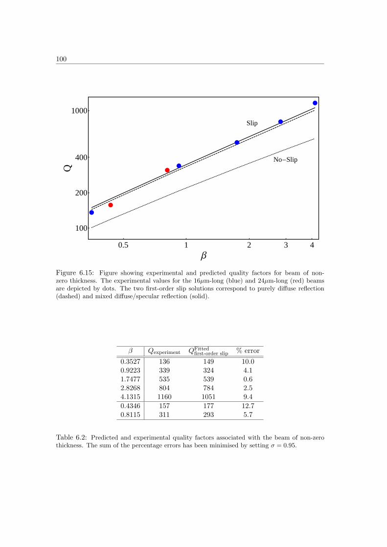
100
No-Slip
Slip
0.5 1 2 3 4
100
200
400
1000
Β
Q
Figure 6.15: Figure showing experimental and predicted quality factors for beam of non-zero thickness. The experimental values for the 16µm-long (blue) and 24µm-long (red) beamsare depicted by dots. The two first-order slip solutions correspond to purely diffuse reflection(dashed) and mixed diffuse/specular reflection (solid).
β Qexperiment QFittedfirst-order slip % error
0.3527 136 149 10.00.9223 339 324 4.11.7477 535 539 0.62.8268 804 784 2.54.1315 1160 1051 9.40.4346 157 177 12.70.8115 311 293 5.7
Table 6.2: Predicted and experimental quality factors associated with the beam of non-zerothickness. The sum of the percentage errors has been minimised by setting σ = 0.95.

Chapter 6. Beam of Non-Zero Thickness 101
Recall that the actual Knudsen number for the beams is 0.17. The Knudsen number
which minimises the percentage error committed by the predicted quality factors is
Kn = 0.1879. By observation of Eq. (6.56), we see that varying Kn is equivalent to
altering σ. The fitted value of Kn corresponds to a thermal accommodation coefficient of
σ = 0.95. This means that fluid-beam interactions are predominantly diffuse in nature,
with a small degree of specular reflection. This is a particularly interesting result,
since the model we have developed is able to determine the nature of the gas-surface
interaction.


Chapter 7
Concluding Remarks
When a clamped-clamped silicon carbide beam is excited thermoelastically, it ex-
hibits a wide range of in-plane and out-of-plane resonances. Recent experiments con-
ducted by Bargatin et al. [2] involved immersing such beams in a viscous fluid and
measuring the quality factors associated with the displayed resonances. Whilst the ex-
perimental data could be fitted, a comprehensive mathematical model accounting for
the underlying physical principles remained elusive. This was the motivation that led
to the formulation of the theory presented in this thesis.
In order to understand the behaviour of the nanoelectromechanical devices used,
we have tackled the problem from two distinct angles. The first involved analysing the
devices using beam theory in order to predict the resonant frequencies. There was very
good agreement between experimental results and the predicted values, both for the
in-plane and out-of-plane modes. The second, and considerably larger component of
this thesis was to formulate a model able to predict the quality factors observed by
Bargatin et al.. On our journey towards the full theoretical model we have adopted
many “simple” models which capture key elements of the underlying physics one by one.
Since the beams are extremely small (width 400nm and thickness 80nm), it is necessary
to move away from a description which relies entirely on classical continuum mechanics.
Indeed, we have found that the effects associated with slip are quite significant.
Chapters 5 and 6 constitute original research. Recall in Chapter 5, we found that
the beam of zero thickness, subject to the no-slip condition yielded quality factors which
103

104
were reasonably accurate. The leading face of the beam and the inclusion of slip serve
to diminish and enhance the quality factors, respectively. Consequently, we conclude
that these two mechanics provide competing effects for the infinitely thin blade subject
to no-slip.
The full theoretical model accounting for the non-zero thickness of the beam as well
as the effects of slip produced results which agreed remarkably well with experimental
values. Interestingly, the predicted values are independent of the amplitude of vibration
and the boundary conditions at the ends of the beam. In addition, we have also been
able to draw some conclusions about the nature of the surface of the beams. We have
found that the coefficient of thermal accommodation at the surface is approximately
σ = 0.95 representing predominantly diffuse reflection.
Further Work
There are several aspects of this problem which could be pursued in the future. As
with any model attempting to account for physical observations, rigorous testing and
repetition of experiments is required. The data available to us is limited to beams of
only one aspect ratio. Further testing could be undertaken for various aspect ratios
since the model presented allows for arbitrary rectangular cross-section.
As mentioned in Appendix B, the corners of the beam represent a flow regime
distinct from all other regions. A rigorous asymptotic analysis of this region could be
undertaken, accounting for the infinitesimal length scale. Having said this, the Navier
slip condition employed by us has proved very successful in capturing the behaviour at
the corners.
Beams of different cross-sectional geometry could be explored without too much
difficulty. The construction of the present model has been done using a general boundary
integral formulation. As such, it would be quite achievable to look at triangular or
trapezoidal cross-sections.
In order to improve the rate of convergence of the slip solutions in Chapter 6,
we could employ a different method of discretization in order to capture the strong
singularities at the edges more effectively.

Appendix A
Richardson Extrapolation
Richardson extrapolation is a method used to accelerate the rate of convergence of
a sequence. This is of particular interest to us since it enables us to obtain extremely
accurate results for the computed vorticity and pressure, whilst only having to solve the
matrix-vector equations a few times with modest mesh sizes. The process of Richardson
extrapolation is outlined by Hornbeck [13].
Suppose we have some value I which we wish to evaluate. Suppose also that the
outcome of some numerical method yields an approximation I to the desired value I.
We write
I = I − C(∆x)p −D(∆x)2p − E(∆x)3p − . . . , (A.1)
where ∆x is the mesh size used for the quadrature method and p is the exponent of the
dominant error term. The functions C, D and E are independent of ∆x. If we take
two different mesh sizes, ∆x1 and ∆x2, then the corresponding estimates of I are given
by I1 and I2 respectively. The above equation then becomes
I1 = I − C(∆x1)p −D(∆x1)2p − E(∆x1)3p − . . . , (A.2)
I2 = I − C(∆x2)p −D(∆x2)2p − E(∆x2)3p − . . . . (A.3)
Upon setting ∆x1 = 2∆x2, we find that Eq. (A.2) can be written as
I1 = I − 2pC(∆x2)p − 22pD(∆x2)2p − 23pE(∆x2)3p − . . . . (A.4)
105

106
It follows that
2pI2 − I12p − 1
= I + 2pD(∆x2)2p +2p(22p − 1)
2p − 1E(∆x2)3p + . . . . (A.5)
We now have a new estimate for I obtained using I1 and I2 in which the error
term involving (∆x)p has vanished. This estimate will thus be more accurate than
either of the two initial guesses. The above procedure can be repeated provided we
have estimates for I on additional mesh spacings. We can readily generalise to the
case with l starting guesses for I, evaluated on meshes which differ by a factor of two.
That is, ∆x1 = 2∆x2 = 4∆x3 = 8∆x4 = . . .. If each starting value is given by I1,i for
i = 1, . . . , l, then we can perform an iteration according to the following rule:
Il,k =2p(l−1)Il−1,k+1 − Il−1,k
2p(l−1) − 1. (A.6)
This will yield l − 1 new estimates for I, each with the dominant error term re-
moved. We can iterate using Eq. (A.6) until we have only one value left. This will be a
very good approximation to the actual value of I since each iteration involves removing
the dominant error term.

Appendix B
Matched Asymptotic Solutions
B.1 Beam of Zero Thickness
We now attempt a matched asymptotic expansion for the beam of zero thickness.
We will only consider the first-order correction arising due to the slip. In a similar
fashion to Chapter 4, we perform a perturbation expansion of the appropriate variables.
These can be written as
ψ = ψ(0) + ηψ(1) +O(η2), (B.1)
ω = ω(0) + ηω(1) +O(η2). (B.2)
The first-order slip condition is given by
U (0) + ηU (1) +O(η2) = Ubeam + aγη
(∂U (0)
∂z′+ η
∂U (1)
∂z′+O(η2)
),
where both sides of the above equation are evaluated at z′ = 0. Upon substitution of
Eqs. (B.1) and (B.2) into the above equation, we can equate the coefficients of η to
obtain
O(1) :∂ψ(0)
∂z′
∣∣∣∣z=0
= U (0) = Ubeam,
O(η) :∂ψ(1)
∂z′
∣∣∣∣z=0
= U (1) = aγ∂U (0)
∂z′= −aγω(0).
107

108
Recall that the streamfunction of the fluid is given by Eq. (5.7) where the term
involving the pressure vanishes by symmetry for in-plane modes. Upon differentiation
with respect to the normal coordinate z′, we obtain
∂ψ(y′, z′)∂z′
=∫ a
−a∆ω(y)Ψzz′(y, 0; y′, 0)dy.
Upon substitution of Eqs. (B.1) and (B.2) into the above integral equation, and
equating different orders of η, we obtain the following coupled integral equations:
O(1) :∫ a
−a∆ω(0)(y)Ψzz′(y, 0; y′, 0)dy =
∂ψ(0)
∂z′
∣∣∣∣z=0
= Ubeam, (B.3)
O(η) :∫ a
−a∆ω(1)(y)Ψzz′(y, 0; y′, 0)dy =
∂ψ(1)
∂z′
∣∣∣∣z=0
= −aγω(0)(y). (B.4)
Notice that the zeroth-order vorticity can be solved directly using Eq. (B.3). This
gives the vorticity associated with the no-slip condition and has already been found
in Chapter 5. The first-order correction to the vorticity can then be found recursively
using Eq. (B.4). The fluid vorticity jump across the blade to first-order in η is then
given by
∆ω = ∆ω(0) + η∆ω(1).
From a practical point of view, this procedure is not particularly difficult. The
necessary mathematical machinery has already been set up in Chapter 5. We are
required to solve the matrix system in Eq. (5.21) again but with a new right-hand side.
The kernel function inside the integrand remains the same and so the kernel matrix
remains unchanged. We must solve the equation
MΛ(1) = −γΛ(0), (B.5)
where M is precisely the same matrix as in Eq. (5.21). Several problems arise when
we implement the solution method just outlined, both in qualitative and quantitative
manners.
Let us consider what happens to the calculated vorticity jump upon inclusion of
the first-order correction term. Fig. B.1 contains plots showing Λ(0)(ξ) and Λ(0)(ξ) +
ηΛ(1)(ξ), the scaled vorticity jumps to zeroth and first-order respectively. Note that

Chapter B. Matched Asymptotic Solutions 109
the scaling has been performed in the same way as in Chapter 5. There are two main
issues with these plots. Note that the first-order correction actually serves to increase
the vorticity over the bulk of the blade face. This is problematic since it would suggest
that viscous losses actually increase upon inclusion of slip! Furthermore, the vorticity
exhibits a sharp jump at the edges from ±∞ to ∓∞. Suppose we were to put these
concerns aside briefly and proceed to integrate the dotted curves across the face of the
blade. The plots in Fig. B.1 represent the solution corresponding to N = 50 subdi-
visions. As we increase N , we actually find that convergence is not achieved. The
singularities near the edges of the blade are so strong that as the solutions approach
ξ = ±1, the area enclosed beneath the curves does not converge. This suggests that
there is some fundamental problem with the formulation of the solution since we have
obtained a singularity which is not integrable.
Let us consider the nature of the singularity in the first-order vorticity. Recall
that solutions arising from inversion of the matrix in Eq. (5.21) exhibit a square-root
singularity at the edges of the blade. If we are to re-use the matrix equation with Λ(0)
on the right-hand side, then the solution obtained will have have a stronger singularity
at the edges since the square-root singularity will have been counted twice. Indeed, a
singularity will be observed which is not integrable. Thus, there exists some fundamen-
tal flaw in the entire procedure of performing a matched asymptotic expansion in this
way.

110
First order
Zeroth order
-1.0 -0.5 0.5 1.0Ξ
-20
-10
10
20
30
40ReHLL
(a)
First order
Zeroth order
-1.0 -0.5 0.5 1.0Ξ
-40
-30
-20
-10
10
20ImHLL
(b)
Figure B.1: Real and imaginary components of the vorticity jump across the infinitely thinblade. The bold curves represent the zeroth-order solution obtained in Chapter 5 while thedashed curves show matched asymptotic expansions correct to first-order. These results areplotted for dimensionless frequency β = 0.3527, Kn = 0.17 and have been solved with N = 50subdivisions.

Chapter B. Matched Asymptotic Solutions 111
So far we have matched two solutions corresponding to inner and outer components
of the flow, for small Knudsen number Kn. This worked perfectly for the infinite plate
solution obtained in Chapter 4, but presents difficulties for the beam of zero thickness.
In performing the matched asymptotic expansion, we have treated the fluid as con-
sisting of two distinct flow regimes; close to the blade and far away from the blade.
Consider however, the region at the leading edge of the blade. In this region, the effec-
tive length scale is δ ≈ 0, depicted in Fig. B.2, while the thickness of the kinetic layer is
still O(η). Thus, the Knudsen number at the leading edge is Kn →∞ which represents
free molecular flow. Obviously an expansion in small Kn will not be valid here. We
certainly would not expect the vorticity to exhibit a non-integrable singularity in such
circumstances. To handle the leading edge of the blade appropriately, we would need
to perform a matched asymptotic expansion for the three distinct flow regions depicted
in Fig. B.2.
η δ
Continuum
Knudsen layer Free
molecular
Figure B.2: Figure showing the three distinct flow regions
We do not proceed with this analysis since it is incredibly complex. Instead, we
will stand by our solution obtained in Chapter 5 where the Navier slip condition was
used. As previously mentioned, this slip condition automatically accounts for both the
Kn → 0 and Kn →∞ limits, enabling its use across the entire face of the blade.

112
B.2 Beam of Non-Zero Thickness
The process of searching for a matched asymptotic expansion across two distinct
flow regimes proved to be successful for the infinite plate model but fruitless for the
beam of zero thickness. We may also wonder whether this approach is likely to work for
the beam of non-zero thickness. Suppose we expand the relevant variables presented in
Chapter 6 in terms of small η (or equivalently Kn) to obtain
ψ = ψ(0) + ηψ(1) +O(η2), (B.6)
ω = ω(0) + ηω(1) +O(η2), (B.7)
p = p(0) + ηp(1) +O(η2). (B.8)
Combining the above equations with Eq. (6.30) and equating the different orders
of η, we obtain the following:
O(1) : ψ(0) = −Ubeamz′ +
∫Cbeam
[− ω(0)Ψn +
1µp(0)Ψl
]dl, (B.9)
O(η) : ψ(1) =∫Cbeam
[− aγω(0)Ω− ω(1)Ψn +
1µp(1)Ψl
]dl. (B.10)
In the latter of the above equations, we have made use of the slip condition so
that ψ(1)n = aγω(0). Equation (B.9) corresponds to the no-slip boundary condition. We
have already solved this problem in Chapter 6 to obtain the vorticity ω(0) and pressure
p(0), correct to O(1). With ω(0), we can use Eq. (B.10) subject to the appropriate slip
boundary condition to recursively determine the first-order corrections to the vorticity
and pressure. This appears to be a feasible way of incorporating slip into the model
of the beam of non-zero thickness. However, the difficulties that became evident in
Section B.1 also arise here. Although we do not explicitly present the results, we find
that through using the zeroth-order results to compute the first-order correction, the
singularities in the vorticity and pressure become stronger. As in Section B.1, we find
that the computed results are in fact non-integrable. While this solution method may
appear appealing at first, we find that it is fruitless. Its failure can be attributed to the
fact that we have ignored the fluid near the corners of the beam as a third and distinct
flow regime.
Bibliography
[1] Y.T. Yang, C. Callegari, X.L. Feng, K.L. Ekinci, and M. L. Roukes. Zeptogram-
scale nanomechanical mass sensing. Nano Letters, 6(4), 2006.
[2] I. Bargatin, I. Kozinsky, and M. L. Roukes. Efficient electrothermal actuation
of multiple modes of high-frequency nanoelectromechanical resonators. Applied
Physics Letters, 90(9), Feb 26 2007.
[3] J.E. Sader. Frequency response of cantilever beams immersed in viscous fluids
with applications to the atomic force microscope. Journal of Applied Physics,
84(1):64–76, Jul 1 1998.
[4] L.F. Crabtree, G.E. Gadd, N. Gregory, C.R. Illingworth, C.W. Jones, D. Kuche-
mann, M.J. Lighthill, R.C. Pankhurst, L. Rosenhead, L. Sowerby, J.T. Stuart, E.J.
Watson, and G.B. Whitham. Laminar Boundary Layers. Oxford University Press,
1963.
[5] E.O. Tuck. Calculation of unsteady flows due to small motions of cylinders in a
viscous fluid. Journal of Engineering Mathematics, 3(1):29–44, 1969.
[6] C.P. Green and J.E. Sader. Small amplitude oscillations of a thin beam immersed
in a viscous fluid near a solid surface. Physics of Fluids, 17(7), Jul 2005.
[7] C.P. Green and J.E. Sader. Torsional frequency response of cantilever beams im-
mersed in viscous fluids with applications to the aomic force microscope. Journal
of Applied Physics, 92(10), Nov 2002.
[8] J.E. Sader, J.W.M. Chon, and P. Mulvaney. Calibration of rectangular atomic
force microscope cantilevers. Review of Scientific Instruments, 70(10):3967–3969,
Oct 1999.
113

114
[9] N.G. Hadjiconstantinou. Oscillatory shear-driven gas flows in the transition and
free-molecular-flow regimes. Physics of Fluids, 17(10), Oct 2005.
[10] G.A. Bird. Molecular Gas Dynamics and the Direct Simulation of Gas Flows.
Oxford University Press, Melbourne, 2003.
[11] C.R. Lilley and J.E. Sader. Velocity profile in the knudsen layer according to the
boltzmann equation. Proceedings of The Royal Society A, 464(2096), 2008.
[12] E.J. Hinch. Perturbation Methods. Cambridge University Press, 1995.
[13] R.W. Hornbeck. Numerical Methods. Quantum Publishers, 1975.
[14] S. Wolfram. Mathematica: a system for doing mathematics by computer. Addison-
Wesley Publishing Co., 1991.
[15] M. Abramowitz and I.A. Stegun. Handbook of mathematical functions. Dover
Publications, New York, 1965.
[16] D. Halliday, R. Resnick, and J. Walker. Fundamentals of physics, extened, with
modern physics. John Wiley and Sons. Inc., New York, 4th edition, 1993.
[17] J.H. Park, P. Bahukudumbi, and A. Beskok. Rarefaction effects on shear driven
oscillatory gas flows: A direct simulation monte carlo study in the entire knudsen
regime. Physics of Fluids, 16(2):317–330, Feb 2004.
[18] S Basak, A Raman, and S.V. Garimella. Hydrodynamic loading of microcantilevers
vibrating in viscous fluids. Journal of Applied Physics, 99(11), Jun 1 2006.
[19] R.D. Knight. Physics for Scientists and Engineers: A Strategic Approach. Pearson
Addison-Wesley, 2008.
[20] H.L. Evans. Laminar Boundary-Layer Theory. Addison-Wesley Publishing Co.,
London, 1968.
[21] C. Pozrikidis. Boundary integral and singularity methods for linearized viscous
flow. Cambridge University Press, Melbourne, 1992.
[22] H. Power and L.C. Wrobel. Boundary Integral Methods in Fluid Mechanics. Com-
putational Mechanics Publications, Southampton, 1995.

BIBLIOGRAPHY 115
[23] L.D. Landau and E.M. Lifshitz. Fluid Mechanics. Pergamon Press Ltd., London,
1959.
[24] R.L. Daugherty, J.B. Franzini, and E.J. Finnemore. Fluid Mechanics with Engi-
neering Applications. John Wiley and Sons, Inc., 2003.