The dynamical evolution of substructure

Bing Zhang,1P Rosemary F. G. Wyse,1,2P Massimo Stiavelli3P and Joseph Silk4P

1Department of Physics and Astronomy, Johns Hopkins University, 3400 N.Charles Street, Baltimore, MD 21218, USA2School of Physics and Astronomy, University of St Andrews, North Haugh, St Andrews KY16 9SS3Space Telescope Science Institute, 3700 San Martin Drive, Baltimore, MD 21218, USA4Astrophysics, University of Oxford, Keble Road, Oxford OX1 3RH

Accepted 2001 December 21. Received 2001 December 21; in original form 2001 May 9

A B S T R A C T

The evolution of substructure embedded in non-dissipative dark haloes is studied through

N-body simulations of isolated systems, both in and out of initial equilibrium, complementing

cosmological simulations of the growth of structure. We determine by both analytic

calculations and direct analysis of the N-body simulations the relative importance of various

dynamical processes acting on the clumps, such as the removal of material by global tides,

clump–clump heating, clump–clump merging and dynamical friction. The ratio of the

internal clump velocity dispersion to that of the dark halo is an important parameter; as this

ratio approaches a value of unity, heating by close encounters between clumps becomes less

important, while the other dynamical processes continue to increase in importance. Our

comparison between merging and disruption processes implies that spiral galaxies cannot be

formed in a protosystem that contains a few large clumps, but can be formed through the

accretion of many small clumps; elliptical galaxies form in a more clumpy environment than

do spiral galaxies. Our results support the idea that the central cusp in the density profiles of

dark haloes is the consequence of self-limiting merging of small, dense haloes. This implies

that the collapse of a system of clumps/substructure is not sufficient to form a cD galaxy, with

an extended envelope; plausibly, subsequent accretion of large galaxies is required. The post-

collapse system is in general triaxial, with rounder systems resulting from fewer, but more

massive, clumps. Persistent streams of material from disrupted clumps can be found in the

outer regions of the final system, and at an overdensity of around 0.75, can cover 10 to 30 per

cent of the sky.

Key words: galaxies: elliptical and lenticular, cD – galaxies: formation – galaxies: spiral –

galaxies: structure.

1 I N T R O D U C T I O N

In the context of Cold Dark Matter (CDM) dominated, hierarchical

clustering cosmology, large galaxies are formed from the merging

and accretion of small, less massive progenitors (clumps). The

exact role played by this substructure in the formation of galaxies is

still unclear, and there remain unresolved several very important

and fundamental issues that are closely related to the role of these

clumps.

The angular momentum content of galaxies is a fundamental

parameter. Cosmological N-body simulations have verified the

proposal that tidal torques between protogalaxies generate angular

momentum (Peebles 1969), and have shown that the dimensionless

spin parameter l ; JjEj1=2

G 21M 25=2 has a well-defined mean

value of ,0.06, independent of the details of the power spectrum

of density fluctuations (Efstathiou & Jones 1979; Aarseth & Fall

1980; Barnes & Efstathiou 1987; Warren et al. 1992; Steinmetz &

Bartelmann 1995; Cole & Lacey 1996). Since the spin parameter l

is much smaller for present-day ellipticals – indeed equal to the

value of ,0.06 of a typical dark halo – than is the value of l for

spirals, while the effective radius for spirals is comparable to that

of ellipticals at a given luminosity (Fall 1980), it is important to

know how the ellipticals succeed in losing angular momentum,

compared to the expectation of smooth collapse and spin-up within

a dark halo (Fall & Efstathiou 1980) while still dissipating the same

amount of binding energy as do protospirals. On the other hand,

there exists an angular momentum problem in that while discs are

formed in fully self-consistent hierarchical-clustering simulations,

the angular momentum transport inherent in the merging process

produces discs that are too centrally concentrated and contain too

little angular momentum compared with observed spirals (e.g.

PE-mail: bingz@epicsystems.com (BZ); wyse@pha.jhu.edu (RFGW);

mstiavel@stsci.edu (MS); silk@astro.ox.ac.uk (JS)

Mon. Not. R. Astron. Soc. 332, 647–675 (2002)

q 2002 RAS

Navarro & Benz 1991; Evrard, Summers & Davis 1994; Vedel,

Hellsten & Sommer-Larsen 1994; Navarro & Steinmetz 1997).

Indeed, standard analytic and semi-analytic models of the

formation of spiral galaxies show that extended discs, as observed,

form through detailed angular momentum conservation, with

protodisc material retaining the same value of specific angular

momentum as the dark halo (e.g. White & Rees 1978; Fall &

Efstathiou 1980; Gunn 1982; Jones & Wyse 1983; Dalcanton,

Spergel & Summers 1997; Mo, Mao & White 1998; Zhang & Wyse

2000; Silk 2001). Hence models must retain angular momentum

for spirals, while losing it for ellipticals. Mergers and the

associated gravitational torques and angular momentum transport

clearly play a role. However, detailed merger simulations of two

disc galaxies have shown that there are difficulties with the

simplest merger picture of how ellipticals form (Bendo & Barnes

2000; Cretton et al. 2001), in that equal-mass mergers seem to

produce too much kinematic misalignment, while in unequal-mass

mergers the strong signatures of the more massive disc survive.

What are the effects of substructure such as gas clouds, stellar

(globular?) clusters, dwarf galaxies or subhaloes which fall later

into the galactic-scale potential well? Do they significantly change

the angular momentum distribution and further change the final

galaxy classification? An analytical approach will have difficulties

in dealing with this problem, although the secondary infall model is

successful in describing the smooth post-collapse halo profile

(Gunn & Gott 1972; Gunn 1977; Filmore & Goldreich 1984;

Hoffman & Shaham 1985; Bertschinger & Watts 1988; Zaroubi,

Naim & Hoffman 1996). However, numerical simulations have the

capability of treating the formation and the non-linear evolution of

dark haloes in a cosmological context (Quinn, Salmon & Zurek

1986; Quinn & Zurek 1988; Zurek, Quinn & Salmon 1988;

Dubinski & Carlberg 1991; Warren et al. 1992). These studies

show that the angular momentum and binding energy are indeed

redistributed, in an orderly manner, during the relaxation of the

haloes (Quinn & Zurek 1988). Further, during the merging process

inherent in hierarchical clustering, baryonic substructure can lose

angular momentum to the dark halo (Frenk et al. 1985; Barnes

1988; Zurek et al. 1988; Navarro, Frenk & White 1995; Navarro &

Steinmetz 1997). Zurek et al. suggest that whether the baryonic

clumps are gas clouds (and hence dissipative) or stellar could be an

important criterion in determining whether the forming galaxy will

become a spiral or an elliptical.

Proposed solutions to the problem with discs, within the context

of CDM cosmologies, have included delaying the onset of disc

formation until after the merging process is essentially complete,

by appeal to suitable ‘feedback’ from the first stars (Weil, Eke &

Efstathiou 1998), but this solution must address the old age for disc

stars in the solar neighbourhood (e.g. Edvardsson et al. 1993; Wyse

1999) and in the outer parts of the M31 disc (Ferguson & Johnson

2001), in addition to the observation of apparently fully formed

discs at redshifts above unity (Brinchmann & Ellis 2000) with a

Tully–Fisher relation that is essentially indistinguishable from that

of present-day discs, apart from passive evolution. The density and

mass of the substructure are clearly important, and a major

motivation for the present work is to quantify the effects of

substructure of a range of each. Further, when is substructure

disrupted and why?

Another issue we seek to clarify is how much of the angular

momentum change seen in the cosmological simulations is due to

the boundary conditions, namely that the system under study is not

closed. It is hard to separate the effects of the real angular

momentum transfer from clumps to halo from the angular

momentum gain by the accretion of material or the torques applied

by the neighbouring environment or the later infall of dark matter.

Thus it is worthwhile to study, as here, the evolution of angular

momentum in isolated systems. In the isolated N-body simulations

by Barnes (1988) of the encounter of two galaxies, it is found that

the dark halo can extract some angular momentum from other

components.

In this paper we shall extend such N-body studies of the

dynamical evolution to analyse the evolution of a system of clumps

in a larger, smooth, isolated system. Our simulations have

relevance beyond a forming protogalaxy. We may address the

dynamical processes occurring in a virialized system with

substructure, such as a cluster of galaxies or a single galaxy and

its retinue of dwarf companion galaxies. The relative importance of

the effects of the dissipationless collapse of the overall system,

tidal disruption of clumps, dynamical friction of clumps, clump–

clump heating and merging can possibly be related to the formation

of cD galaxies in clusters of galaxies, to the formation of central

density cusps in dark haloes, to the triaxial nature of dark haloes, to

the formation of substructure composed of disrupted debris in the

outer halo regions of galaxies, etc. Thus we initiated a consistent

comparison among these dynamical processes in the context of

galaxy formation.

In Section 2 we present the parameters of our N-body

simulations. Section 3 contains a discussion of our expectations

for the dynamics of the substructure based on analytic calculations

and comparisons with the N-body simulations, while Section 4

discusses the angular momentum content and transport. The

internal kinematics of the different components are discussed in

Section 5, while their morphology is discussed in Section 6.

Section 7 summarizes our conclusions. The more technical aspects

are given in the appendices.

2 T H E N - B O DY M O D E L S

2.1 The technique

We adopt a numerical N-body code based on the hierarchical tree

algorithm (Barnes & Hut 1986; Hernquist 1987). Our simulations

study the dynamical evolution of a number of clumps embedded in

a smooth dark halo. Due to the collisionless property of the

particles used in our N-body simulation, it should be emphasized

that the clump can represent either stellar or dark matter, depending

on our interpretation of the physical entity. The initial dark halo

profile is modelled with either the Hernquist profile (Hernquist

1990) or the Plummer profile (Plummer 1911), the details of which

are given in Appendix A. The Hernquist profile, with r , r 21 at

the centre and r , r 24 at large radius, was introduced as being,

when projected, close to the observed surface brightness profiles of

elliptical galaxies, and is close to the mass profile seen in

hierarchical clustering simulations (the NFW profile; Navarro,

Frenk & White 1997), which has a cuspy centre, r , r 21 (though

flatter than the ,r 21.5 behaviour of high-resolution simulations;

Ghigna et al. 2000), and r , r 23 at large radius. The Plummer

profile has close to a harmonic potential in the core (only slowly

varying density) and r , r 25 at large radius. In all realizations,

each clump is simulated with a Plummer profile.

We ran simulations of systems in initial equilibrium plus out-of-

equilibrium systems that underwent an initial collapse. In order to

study the angular momentum behaviour of the clumps and the dark

halo, we require that the system contain enough angular

momentum, consistent with the cosmological initial conditions

648 B. Zhang et al.

q 2002 RAS, MNRAS 332, 647–675

expected, i.e., l , 0:1 (e.g. Efstathiou & Jones 1979; Barnes &

Efstathiou 1987). First, we build the dark halo with no streaming

velocity. Then, we add some angular momentum about the z

direction, which is defined to be the axis of the halo. The orbital

rotation velocity added to each particle is the component projected

on the equatorial plane of a constant fraction, b, of the circular

velocity where the particle is located, i.e., V rot ¼ bVcðrÞ cos u,

where u is the angle between r and z. We further stretch the

spherical profile to an oblate profile with ellipticity e0 ¼ 0:53

(Warren et al. 1992). Assuming, if the system is virialized, that the

flattening is caused only by the addition of rotation, we adopt

the empirical relation b ¼ffiffiffiffiffiffiffiffiffie0/5p

, which may be seen by noting the

scaling of the rotation parameter v0/s/ffiffiffiffiffie0p

for isotropic systems

flattened by rotation (Binney & Tremaine 1987). With this choice

of b, the initial spin parameter of the halo in the virialized

simulations (with the virial ratio 2T/W , 1, where T is the total

kinetic energy and W is the total potential energy) is l , 0:16. The

collapse simulation models (with the virial ratio 2T/W , 0:1Þ have

l , 0:07. In order to achieve an initial condition suitable for pre-

collapse, i.e., with small 2T/W , we decrease the total velocity of

the dark halo particles and the velocity of each clump by a factor offfiffiffiffiffi10p

for 2T/W , 0:1.

No internal rotation is added to the clumps, which are spherical.

The distribution of clumps is chosen to follow the dark halo profile

with similar treatment of the flattening and rotation velocity. For

the simulation models with the same number of clumps, we require

the orbital characteristics for the clumps to be the same, with the

exception of models B and E (see Table 1).

2.2 The parameters and units

The parameter values of interest for our simulations are given in

Table 1. The total number of particles in our simulations ranged

from 20 000 to 120 000, with smooth dark halo particles and clump

particles having an equal mass. The total number of clumps, nc,

varied from 5 to 80, and the total clump mass fraction, f, varied

from 5 to 100 per cent. These ranges were chosen to study the

effect of clumpiness on the outcome of the simulations. The core

radius of a clump (a Plummer sphere) is set to achieve the chosen

density contrast, rcl/r0, the ratio of the mean density within the

half-mass radius of the clump to that of the whole system (dark

matter plus the clumps). We vary the density parameter rcl/rDM

[with rcl/r0 ¼ ð1 2 f Þrcl/rDM� over the range of 3 to 64 in our

simulations, to study the effects of global tides in disrupting the

clumps. A value of 3 for the density contrast is the minimum

expected for a system to withstand global tides (the Roche

criterion).

The total mass of the system is normalized to be unity. The

unit of distance is the core size of the dark halo ða ¼ 1; see

Appendix A), and we further set the gravitation constant G ¼ 1.

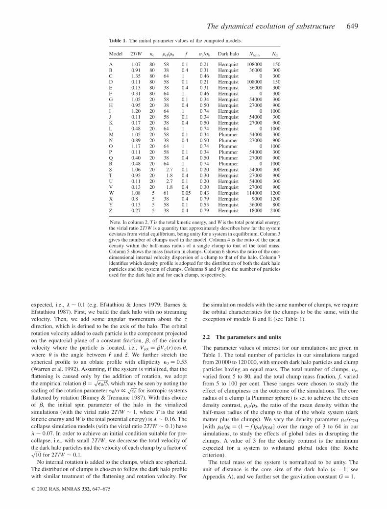
Table 1. The initial parameter values of the computed models.

Model 2T/W nc rcl/r0 f sc/sh Dark halo Nhalo Ncl

A 1.07 80 58 0.1 0.21 Hernquist 108000 150B 0.91 80 38 0.4 0.31 Hernquist 36000 300C 1.35 80 64 1 0.46 Hernquist 0 300D 0.11 80 58 0.1 0.21 Hernquist 108000 150E 0.13 80 38 0.4 0.31 Hernquist 36000 300F 0.31 80 64 1 0.46 Hernquist 0 300G 1.05 20 58 0.1 0.34 Hernquist 54000 300H 0.95 20 38 0.4 0.50 Hernquist 27000 900I 1.20 20 64 1 0.74 Hernquist 0 1000J 0.11 20 58 0.1 0.34 Hernquist 54000 300K 0.17 20 38 0.4 0.50 Hernquist 27000 900L 0.48 20 64 1 0.74 Hernquist 0 1000M 1.05 20 58 0.1 0.34 Plummer 54000 300N 0.89 20 38 0.4 0.50 Plummer 27000 900O 1.17 20 64 1 0.74 Plummer 0 1000P 0.11 20 58 0.1 0.34 Plummer 54000 300Q 0.40 20 38 0.4 0.50 Plummer 27000 900R 0.48 20 64 1 0.74 Plummer 0 1000S 1.06 20 2.7 0.1 0.20 Hernquist 54000 300T 0.95 20 1.8 0.4 0.30 Hernquist 27000 900U 0.11 20 2.7 0.1 0.20 Hernquist 54000 300V 0.13 20 1.8 0.4 0.30 Hernquist 27000 900W 1.08 5 61 0.05 0.43 Hernquist 114000 1200X 0.8 5 38 0.4 0.79 Hernquist 9000 1200Y 0.13 5 58 0.1 0.53 Hernquist 36000 800Z 0.27 5 38 0.4 0.79 Hernquist 18000 2400

Note. In column 2, T is the total kinetic energy, and W is the total potential energy;the virial ratio 2T/W is a quantity that approximately describes how far the systemdeviates from virial equilibrium, being unity for a system in equilibrium. Column 3gives the number of clumps used in the model. Column 4 is the ratio of the meandensity within the half-mass radius of a single clump to that of the total mass.Column 5 shows the mass fraction in clumps. Column 6 shows the ratio of the one-dimensional internal velocity dispersion of a clump to that of the halo. Column 7identifies which density profile is adopted for the distribution of both the dark haloparticles and the system of clumps. Columns 8 and 9 give the number of particlesused for the dark halo and for each clump, respectively.

The dynamical evolution of substructure 649

q 2002 RAS, MNRAS 332, 647–675

With these units and as detailed in Appendix A, the mean

crossing time for a Hernquist halo is 5.3, while that for a Plummer

halo is 2.1, and the simulations are run for ,25 crossing times, or

approximately a Hubble time in physical units.

It is convenient to express some of our parameters, such as the

clump mass fraction f, the number of clumps nc, density contrast of

each clump rcl/r0, and crossing time t12hc, in terms of dimensionless

quantities. From our definition of the density contrast of the clump,

the ratio of the half-mass radius of a clump to that of the whole

system can be written as

r12c/r1

2h ¼ f 1=3n21=3

c

rcl

r0

� �21=3

: ð1Þ

The ratio of the one-dimensional internal velocity dispersion of

the clump and the halo is

sc/sh ¼v1

2c

v12h

¼r1

2c

r12h

t12hc

t12cc

¼r1

2c

r12h

!rcl

r0

� �1=2

:

This can be further written as

sc/sh ¼ f 1=3n21=3c

rcl

r0

� �1=6

: ð2Þ

2.3 Numerical effects

As demonstrated in Appendix B, while there may well be spurious

clump heating effects in our simulations, due to the limited number

of particles used, they do not pose a problem for our analysis. The

softening-length in the treecode is set at rs ¼ 0:5r12clN

21=3cl , where

Ncl is the number of particles used in each clump. This relatively

large value is chosen to suppress the unphysical two-body

relaxation (White 1978), which otherwise could occur due to the

small number of particles used in each clump (ranging from 150 to

2400).

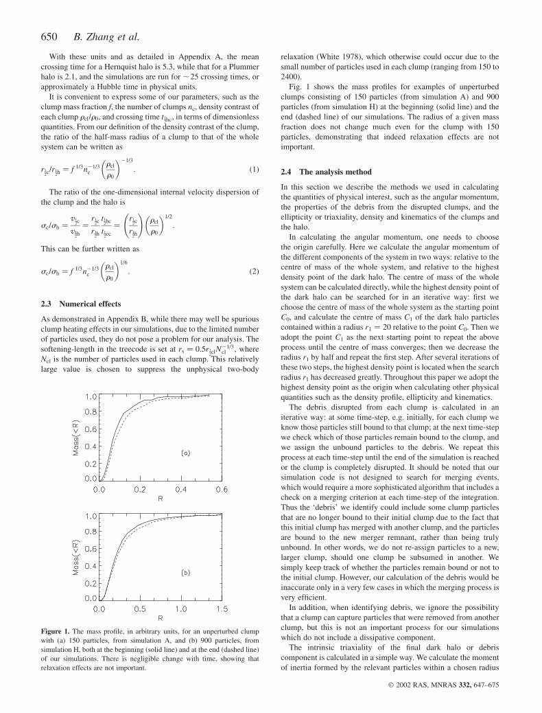
Fig. 1 shows the mass profiles for examples of unperturbed

clumps consisting of 150 particles (from simulation A) and 900

particles (from simulation H) at the beginning (solid line) and the

end (dashed line) of our simulations. The radius of a given mass

fraction does not change much even for the clump with 150

particles, demonstrating that indeed relaxation effects are not

important.

2.4 The analysis method

In this section we describe the methods we used in calculating

the quantities of physical interest, such as the angular momentum,

the properties of the debris from the disrupted clumps, and the

ellipticity or triaxiality, density and kinematics of the clumps and

the halo.

In calculating the angular momentum, one needs to choose

the origin carefully. Here we calculate the angular momentum of

the different components of the system in two ways: relative to the

centre of mass of the whole system, and relative to the highest

density point of the dark halo. The centre of mass of the whole

system can be calculated directly, while the highest density point of

the dark halo can be searched for in an iterative way: first we

choose the centre of mass of the whole system as the starting point

C0, and calculate the centre of mass C1 of the dark halo particles

contained within a radius r1 ¼ 20 relative to the point C0. Then we

adopt the point C1 as the next starting point to repeat the above

process until the centre of mass converges; then we decrease the

radius r1 by half and repeat the first step. After several iterations of

these two steps, the highest density point is located when the search

radius r1 has decreased greatly. Throughout this paper we adopt the

highest density point as the origin when calculating other physical

quantities such as the density profile, ellipticity and kinematics.

The debris disrupted from each clump is calculated in an

iterative way: at some time-step, e.g. initially, for each clump we

know those particles still bound to that clump; at the next time-step

we check which of those particles remain bound to the clump, and

we assign the unbound particles to the debris. We repeat this

process at each time-step until the end of the simulation is reached

or the clump is completely disrupted. It should be noted that our

simulation code is not designed to search for merging events,

which would require a more sophisticated algorithm that includes a

check on a merging criterion at each time-step of the integration.

Thus the ‘debris’ we identify could include some clump particles

that are no longer bound to their initial clump due to the fact that

this initial clump has merged with another clump, and the particles

are bound to the new merger remnant, rather than being truly

unbound. In other words, we do not re-assign particles to a new,

larger clump, should one clump be subsumed in another. We

simply keep track of whether the particles remain bound or not to

the initial clump. However, our calculation of the debris would be

inaccurate only in a very few cases in which the merging process is

very efficient.

In addition, when identifying debris, we ignore the possibility

that a clump can capture particles that were removed from another

clump, but this is not an important process for our simulations

which do not include a dissipative component.

The intrinsic triaxiality of the final dark halo or debris

component is calculated in a simple way. We calculate the moment

of inertia formed by the relevant particles within a chosen radius

Figure 1. The mass profile, in arbitrary units, for an unperturbed clump

with (a) 150 particles, from simulation A, and (b) 900 particles, from

simulation H, both at the beginning (solid line) and at the end (dashed line)

of our simulations. There is negligible change with time, showing that

relaxation effects are not important.

650 B. Zhang et al.

q 2002 RAS, MNRAS 332, 647–675

(e.g., half-mass radius). From the eigenvalues of the moment of

inertia I1 , I2 , I3, we can fit the moment of inertia with a triaxial

ellipsoid with the intrinsic axial ratios e1 ¼ b/a and e2 ¼ c/a,

where a $ b $ c. It can be calculated that

e1 ¼

ffiffiffiffiffiffiffiffiffiffiffiffiffiffiffiffiffiffiffiffiffiffiffiffiffiffiffiffiffi2PQ 2 Pþ Q

PQ 2 P 2 Q

s

and

e2 ¼

ffiffiffiffiffiffiffiffiffiffiffiffiffiffiffiffiffiffiffiffiffiffiffiffiffiffiffiffiffi2PQþ P 2 Q

PQ 2 P 2 Q

s;

where P ¼ I1/I2 and Q ¼ I1/I3. The intrinsic axial ratios

calculated in this way can be slightly overestimated compared

to their real values, but provide a consistent comparison among

our simulations. The ellipticity of the projected (surface

density) images of the final dark halo or debris can be

calculated in a more direct way, for a range of viewing angles.

We calculate an isodensity contour map by assigning a

Gaussian density profile to each particle, with width

proportional to the softening length. Then we simply fit the

contour with the ellipse to obtain the axial ratio b/a and the

ellipticity e ¼ 1 2 b/a.

The radial density profile is calculated by dividing the particles

into radial bins, each containing equal numbers of particles (about

16). The velocity dispersion and rotation velocity are calculated by

the conventional approach.

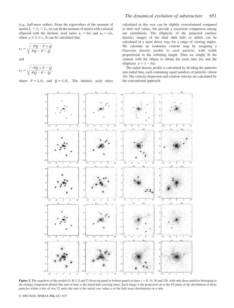
Figure 2. The snapshots of the models G, H, I, S and T (from top panel to bottom panel) at times t ¼ 0, 14, 56 and 126, with only those particles belonging to

the clumpy component plotted (the unit of time is the initial halo crossing time). Each image is the projection on to the XY plane of the distribution of those

particles within a box of size 22 units (the unit is the initial core radius a of the halo mass distribution) on a side.

The dynamical evolution of substructure 651

q 2002 RAS, MNRAS 332, 647–675

3 T H E DY N A M I C S O F C L U M P S

We can study the dynamical evolution of clumps that contain

enough particles. The study of the dynamics of substructure has

applications on both the galaxy-size scale, where star clusters, gas

clouds and dwarf satellite galaxies play the role of clumps (Fall &

Rees 1977), and the galaxy-cluster scale, where galaxies play the

role of clumps (Dressler 1984). It is also related to the

‘undermerging’ problem that has emerged recently, in that high-

resolution CDM cosmological simulations predict too many

surviving dark matter satellites around haloes of the size of our

Galaxy (Klypin et al. 1999; Moore et al. 1999).

The dynamical processes associated with the evolution of these

clumps we shall investigate are global tidal stripping, dynamical

friction, and merging and close encounters between clumps. We

first derive expectations, based on analytic arguments, for the roles

these dynamical processes have played and on which parameters

they depend, for the virialized models. A preliminary comparison

between these theoretical estimates and our simulations is provided

at the end of the section. Snapshots of each model are plotted in

Figs 2–7.

3.1 Analytic expectations

We derived analytic expectations for the amplitudes of the various

processes we believe are operating in the simulations, to gain an

understanding of the results. Many processes are working together,

often with the same net result (disruption of the clumps), which

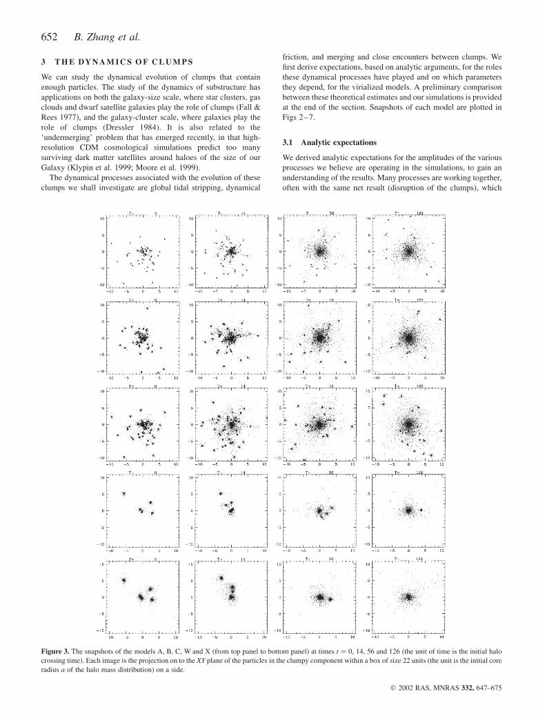
Figure 3. The snapshots of the models A, B, C, W and X (from top panel to bottom panel) at times t ¼ 0, 14, 56 and 126 (the unit of time is the initial halo

crossing time). Each image is the projection on to the XY plane of the particles in the clumpy component within a box of size 22 units (the unit is the initial core

radius a of the halo mass distribution) on a side.

652 B. Zhang et al.

q 2002 RAS, MNRAS 332, 647–675

would greatly complicate the interpretation of the N-body

simulations in the absence of analytic insight.

3.1.1 The effects of global tides

Global tides due to the spatial variation of the underlying large-

scale dark halo potential provide an important mechanism for the

disruption of substructures as they orbit through the dark halo.

Analytical studies of the tidal effect on a clump show that, for a

given clump orbit, the disruption efficiency depends on the ratio

between the clump density to the mean density of halo within the

pericentre of the clump orbit (e.g. King 1962; Binney & Tremaine

1987; Johnston, Hernquist & Bolte 1996). The tidal radius of the

clump, during its disruption, is the Roche radius at which its

gravity is equal to the tidal force exerted by the dark halo, which

roughly scales as

rtide ,Mc

Mtot

� �1=3

R; ð3Þ

where R is the pericentre distance. For our simulations, we expect

that the clumps with density contrast ðrcl/r0Þ ¼ 3 should suffer

more efficient tidal disruption than those with ðrcl/r0Þ ¼ 64. For a

clump in a circular orbit at the half-mass radius of the dark halo, the

fraction of mass contained within the tidal radius is ,97 per cent

for ðrcl/r0Þ ¼ 64 and ,74 per cent for ðrcl/r0Þ ¼ 3. Since the

clumps in our models are each represented by a Plummer profile,

which has a fairly constant density core (see Appendix A), while

the dark halo is represented typically by a Hernquist profile, which

has a cuspy central density profile, the minimum pericentre

distance for the approximately constant density core to be

disrupted is ,0.085 for ðrcl/r0Þ ¼ 64 and ,0.72 for ðrcl/r0Þ ¼ 3.

3.1.2 Merging effects

The merging cross-section between a pair of identical spherical

clumps has been studied by Makino & Hut (1997) numerically,

using a variety of mass profiles for the clumps. They find that in a

cluster of clumps with one-dimensional velocity dispersion sh the

number of merging events per unit time per unit volume, Rm, is

given by

Rm ¼18ffiffiffiffipp

1

x 3n 2r2

cviscR0ðxÞ ¼18ffiffiffiffipp

1

x 4n 2r2

cvishR0ðxÞ; ð4Þ

where x ¼ sh/sc, with sh and sc being the one-dimensional

velocity dispersion of the system of clumps (the halo) and the

internal velocity dispersion of a clump respectively, n is the number

density of the clumps within the half-mass radius of the dark halo,

rcvi is the virial radius of the clump, and the dimensionless quantity

R0ðxÞ ¼Ax 2

x 2þB, with A ¼ 12 and B ¼ 0:4 for clumps with a

Plummer profile. Written this way, one can see explicitly a strong

dependence of the merging rate on the parameter x (the ratio of the

internal velocity dispersions of halo and clump).

The number of merging events per unit time, Rm, expected in our

simulations can be estimated by the product ofRm and the volume

within the half-mass radius of the halo profile (equal to the half-

mass radius of the system of clumps). After some algebraic

manipulations using equations (1) and (2) given in Section 2.2 and

the scalings in Appendix A, we obtain

Rm ¼4

3pr3

12hRm . 0:47f 2R0ðxÞ

1

t12hc

: ð5Þ

Thus the number of merging events per halo crossing time is

0.47f 2R0(x), and depends fairly strongly on the clump mass

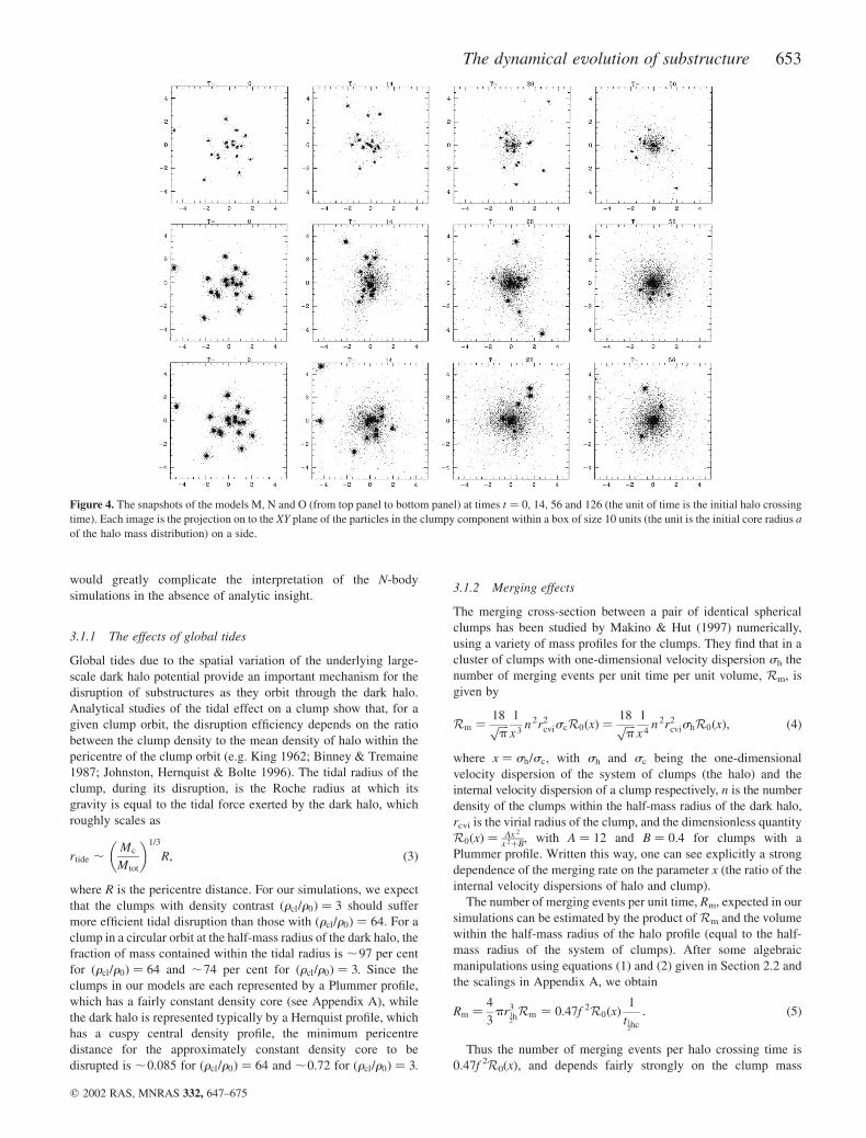
Figure 4. The snapshots of the models M, N and O (from top panel to bottom panel) at times t ¼ 0, 14, 56 and 126 (the unit of time is the initial halo crossing

time). Each image is the projection on to the XY plane of the particles in the clumpy component within a box of size 10 units (the unit is the initial core radius a

of the halo mass distribution) on a side.

The dynamical evolution of substructure 653

q 2002 RAS, MNRAS 332, 647–675

fraction, f, but with only a weak residual explicit dependence on the

parameter x (many parameters are interdependent). In the limit of a

high relative velocity compared to internal velocity dispersion,

x 2 @ 0:4, which is approximately valid for all our models,

R0ðxÞ , 12. This limit does not favour mergers, and results in the

number of merging events per halo crossing time being ,0.05 for

f ¼ 0:1, ,1 for f ¼ 0:4 and ,5 for f ¼ 1.

We can also estimate the merging time-scale for a clump. For a

given clump within the half-mass radius of the halo, the probability

of it merging with another clump per unit time is Rm/n. Thus the

merging time-scale is

tm ¼ n/Rm ¼nc

f 2R0ðxÞt1

2hc: ð6Þ

It should be emphasized that the internal velocity dispersion ratio

of the halo to the clump, x, itself depends on the clump mass

fraction f, the clump number nc and the density contrast rcl/r0 by

equation (2). We can see here that, given the values of the model

parameters, the merging time-scale is only very weakly dependent

on the density contrast, which is instead a crucial factor for the

efficiency of the global tidal stripping. Merging between clumps is

an important effect for large values of the clump mass fraction, f,

and for small numbers of clumps, nc. In our models with f , 0:1,

the merging effect is very small with tm @ 50t12hc, while for larger

f . 0:4, merging can be important, and the minimum merging

time-scale is tm , 1:7t12hc (model I).

The merging rate calculated above is the mean quantity at

the initial half-mass radius. Further, it does not take into account

other dynamical effects, such as global tidal effects and close

encounters, that can greatly decrease the calculated merging rate

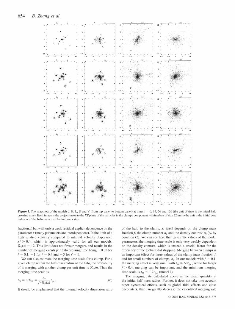
Figure 5. The snapshots of the models J, K, L, U and V (from top panel to bottom panel) at times t ¼ 0, 14, 56 and 126 (the unit of time is the initial halo

crossing time). Each image is the projection on to the XY plane of the particles in the clumpy component within a box of size 22 units (the unit is the initial core

radius a of the halo mass distribution) on a side.

654 B. Zhang et al.

q 2002 RAS, MNRAS 332, 647–675

(Makino & Hut 1997). The effects of global tides can decrease the

merging cross-section by tending to tear apart a pair of clumps

which, if isolated, would have merged. Similarly, the local tides

from a third clump can also act to tear apart a merging pair of

clumps. Furthermore, the subsequent non-linear evolution in the

presence of other more important dynamical processes can make

the estimated merging time-scale change quickly with time. We

will see the limitation of this analytic estimate when we compare

with the simulations below.

3.1.3 Clump–clump heating

Disruption of clumps can also be caused by close encounters with

other clumps. Similarly to the discussion given in Section 2.3.2, we

can estimate this clump disruption time-scale as follows. For a

given clump, the heating rate is

_E ¼4ffiffiffiffipp

G 2m3cn�r2

c

3gshr212c

; ð7Þ

where n is the mean clump number density within the half-mass

radius of the dark halo, and all other parameters are as defined

above. As discussed in Appendix B2, we adopt g , 3 and

�r2c , 2r2

12c. Thus the clump disruption time-scale due to clump–

clump heating is given by

tc–c ¼ 0:03f 24=3n1=3c ðrcl/r0Þ

1=3t12hc: ð8Þ

Thus clump–clump heating is important for a large clump mass

fraction, f, small clump number, nc, and low density contrast,

rcl/r0. We have tc–c , 11t12hc for model A, and tc–c , 1:5t1

2hc for

model B.

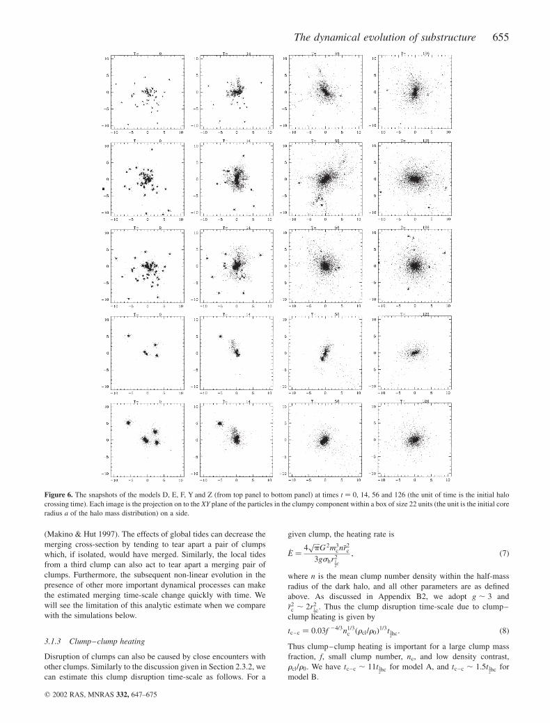
Figure 6. The snapshots of the models D, E, F, Y and Z (from top panel to bottom panel) at times t ¼ 0, 14, 56 and 126 (the unit of time is the initial halo

crossing time). Each image is the projection on to the XY plane of the particles in the clumpy component within a box of size 22 units (the unit is the initial core

radius a of the halo mass distribution) on a side.

The dynamical evolution of substructure 655

q 2002 RAS, MNRAS 332, 647–675

However, we should keep in mind that the above calculation

could overestimate the effects of clump–clump heating. The

choice of �r2c is uncertain. Further, the impulse approximation holds

only for sc/sh ! 1 if the impact parameter b is chosen to be , r12c.

If the encounter time is too long compared with the clump internal

crossing time, particles in the clump may adiabatically respond to

the encounter; hence the encounter could leave no net effects

(Binney & Tremaine 1987). This could possibly explain the

apparent inconsistency between our analytic estimates for the

clump–clump merging effect and the clump–clump heating effect

(equations 6 and 8), in that they both become more important with

large clump mass fraction and small numbers of clumps. From

equation (2), we can see that sc/sh also tends to be large for a large

clump mass fraction and a small number of clumps (provided that

sc/sh ! 1Þ. When sc/sh increases above 0.5, our prediction of the

clump–clump heating effect in equation (8) becomes invalid, and

the clump–clump heating effect will decrease quickly, while the

merging effect will increase continuously.

The above arguments can be understood in terms of three

different regimes, depending on the value of the encounter speed,

basically equivalent to the role of sh. (1) In the case that the

encounter speed V is very high, the two clumps will not merge and

the clumps are just heated somewhat during the fast encounter. (2)

In the case that the encounter speed is just slightly reduced, it can

be envisaged that the chance for merging is slightly increased, and

the heating effect is also slightly enhanced, since the duration of

the encounter is slightly longer. (3) In the case that the encounter

velocity is very low, the merging rate is greatly increased, and

the heating effect can be inhibited, since if the duration of the

encounter is long enough compared to the internal crossing time-

scale in the clump, the clump just adiabatically responds during the

encounter and returns to the initial state after the encounter.

3.1.4 Dynamical friction

Dynamical friction can drive clumps to the centre of the dark halo,

where they can be tidally disrupted more easily. The slowing down

of the clumps also can increase their merging cross-section. At the

same time this process can extract angular momentum from the

clumps, and transfer it to the dark halo. Since Chandrasekhar

(1943) introduced the concept of dynamical friction, namely that

an object moving through an infinite and homogeneous medium

made of small mass particles suffers a drag force, there have been

many studies on this subject by numerical simulations (e.g. White

1978, 1983; Lin & Tremaine 1983; Bontekoe & van Albada 1987;

Zaritsky & White 1988; Hernquist & Weinberg 1989; van den

Bosch et al. 1999) and analytical methods (e.g. Tremaine 1981;

Tremaine & Weinberg 1984; Weinberg 1989; Maoz 1993;

Domınguez-Tenreiro & Gomez-Flechoso 1998; Colpi, Mayer &

Governato 1999; Tsuchiya & Shimada 2000). An overview of past

work is given by Cora, Muzzio & Vergne (1997). In spite of the

difficulties encountered in the study of dynamical friction, many

authors find Chandrasekhar’s formula is a remarkably good

approximation (e.g. Velazquez & White 1999).

Adopting Chandrasekhar’s formula, the deceleration of a clump

is then

dvM

dt¼ 2

vM

tdf

; ð9Þ

where

t21df ¼ 16p2 lnLG 2mpðMc þ mpÞ

Ð vM

0f ðvÞv 2 dv

v3M

; ð10Þ

mp is the mass of a background halo particle, Mc is the mass of the

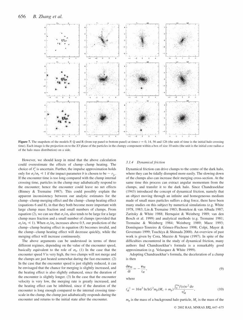
Figure 7. The snapshots of the models P, Q and R (from top panel to bottom panel) at times t ¼ 0, 14, 56 and 126 (the unit of time is the initial halo crossing

time). Each image is the projection on to the XY plane of the particles in the clumpy component within a box of size 10 units (the unit is the initial core radius a

of the halo mass distribution) on a side.

656 B. Zhang et al.

q 2002 RAS, MNRAS 332, 647–675

clump, vM is the velocity of the clump, f ðvÞ is the phase-space

number density of the background halo medium, and L is the ratio

between the maximum and minimum impact parameters bmax/bmin.

Using the values at the half-mass radius, we can immediately see

that the characteristic dynamical friction time,

tdf /nc

f ð1 2 f Þt1

2hc /1

Mcð1 2 f Þt1

2hc; ð11Þ

scales inversely with the mass of a clump ð f /nc, with the total mass

normalized to unity as here).

In applying these formulae to our simulations with virialized

initial conditions, 2T/W , 1, and for which the dark halo is taken

to follow the Hernquist profile, we have chosen to use the phase-

space distribution function given by Hernquist (1990), hence

ignoring the angular momentum dependence of the distribution

function. The phase-space density of the dark halo is then as

detailed in Appendix C. For a clump initially on a circular orbit

at the half-mass radius, the dynamical friction time calculated as

in Appendix C is

tdf;circ ¼0:16nc

f ð1 2 f Þt1

2hc:

Analyses of the orbital eccentricities of substructure in spherical

potentials have found that for isotropic distribution functions the

typical orbital eccentricity is ,0.6 (van den Bosch et al. 1999).

With this value the dynamical friction time is decreased by a factor

of up to 2, and the typical dynamical friction time for our computed

models should then be

tdf , 0:08nc

f ð1 2 f Þt1

2hc: ð12Þ

Thus dynamical friction is more important for a large clump

mass fraction (provided f , 0:5Þ and a small number of clumps,

giving a large mass for each clump. This dependence on f and nc in

a general sense is consistent with that of clump–clump merging in

all parameter ranges and that of clump–clump heating in some

restricted parameter ranges. For our models with nc ¼ 80,

dynamical friction is not important, with tdf . 20t12hc. For our

models with nc ¼ 20, dynamical friction is not important for

f ¼ 0:1, with tdf , 18t12hc, but for f ¼ 0:4 it becomes important,

with tdf , 6:7t12hc. For our models with nc ¼ 5, dynamical friction

is important, with tdf , 8:4t12hc for f ¼ 0:05 and tdf , 1:7t1

2hc for

f ¼ 0:4.

It should be emphasized that efficient dynamical friction leads to

significant angular momentum loss from the clumps, and thus can

drive clumps to the centre, where global tidal effects are stronger.

Thus the net efficiency of tidal stripping by the global potential

includes a dependence on the clump mass fraction and number of

clumps similar to that of dynamical friction.

3.2 Comparison with simulations

It should be noted that the above analysis is mainly applicable to

virialized models. For the pre-collapse models, the disruption of

clumps due to the collapse process itself dominates. For the

Plummer dark halo profile, the details of the calculation of

dynamical friction from Section 3.1.4 are not applicable, but the

scaling should be the same as in the Hernquist models. Thus, for

ease of comparison, the dynamical friction time is normalized to

the crossing time-scale at the half-mass radius, as are all time-

scales.

As noted earlier, all models with the same number of clumps

have the same orbital characteristics for the clumps, with the

exception of models B and E. Thus it should be the different

choices of our three free parameters – the density contrast rcl/r0,

the clump mass fraction f and the number of clumps nc – that are

responsible for differences in the evolution of the different models.

The most important uncertainty in the comparison of the

theoretical predictions with our simulation results comes from two

factors that enter the determination of the theoretical clump–

clump heating time-scale, namely the normalization quantity, �r2c ,

and the use of the impulse approximation even for relatively large

values of sc/sh. However, there are also uncertainties in the

analysis of our simulations. Our code is not designed to follow the

merging events that occur throughout the simulations, and, as

mentioned above, the ‘debris’ includes both particles genuinely

removed from clumps and orbiting freely in the global potential

and the remnants of merging clumps. Thus in our analysis, both

heating and merging produce debris. As a rough estimate of the

mean disruption time-scale of a clump in the simulations, we

simply use the time required for the disruption of half of the clump

mass.

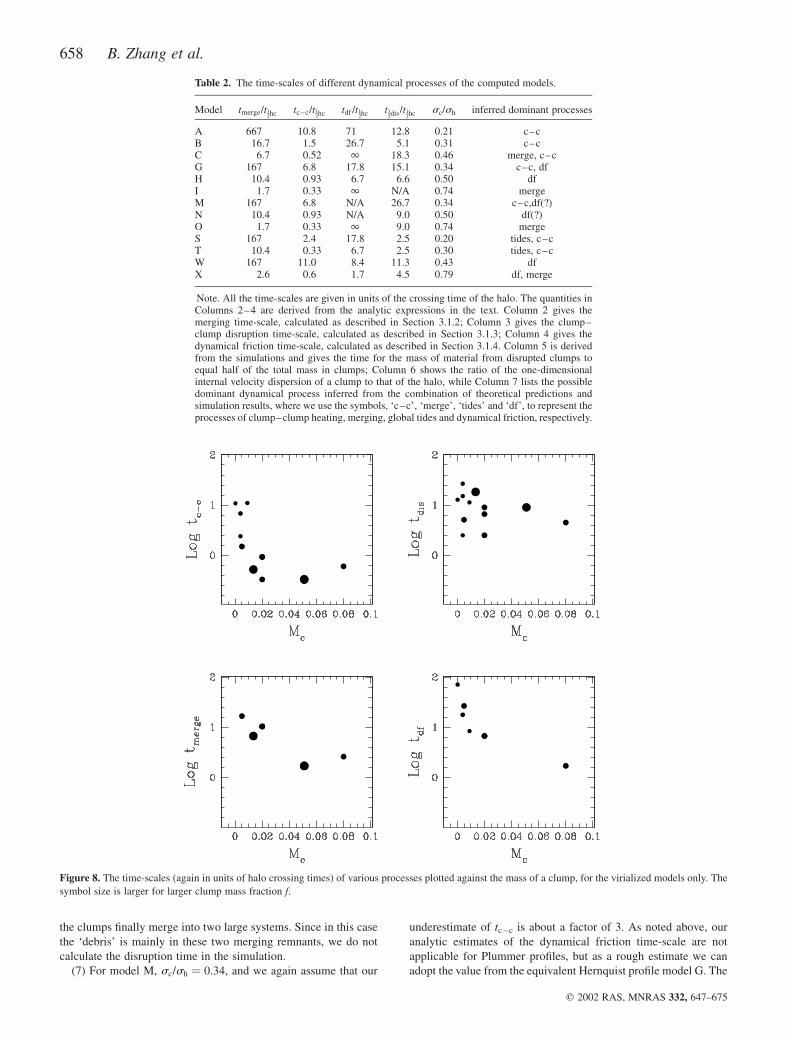
Table 2 lists, for the virialized models only, all the time-scales, in

units of t12hc, calculated from our analytic expressions, together with

the disruption time of half of the mass in clumps measured from

our simulations. The reader should note that the relative

importance of the processes has not be derived from the

simulations explicitly. Fig. 8 shows the dependence of various

processes on the mass of the clump, and also on the mass fraction

in clumps, f, the latter denoted by the symbol size.

The discussion of each virialized model is given in turn

below.

(1) For model A, since sc/sh ¼ 0:21, the impulse approximation

is valid in our calculation of the clump–clump heating time-scale

tc – c. Indeed, the dominant dynamical process is clump–clump

heating, and the analytic prediction is quite consistent with the

simulation result.

(2) For model B, again clump–clump heating is the dominant

dynamical process. However, our analytic estimate of tc – c is a

factor of 3 below the simulation result. This can be understood

since sc/sh ¼ 0:31 and thus we are in the regime of marginal

applicability of the impulse approximation, and we may have

underestimated tc – c.

(3) For model C, we can see sc/sh ¼ 0:46, and thus our

underestimate of tc – c could be significant, possibly by as much as

the factor of 30 needed for consistency with the simulation result. It

is also possible that tmerge is underestimated by the factor of 2

discrepancy with the simulation result. The dominant processes

appear to be merging and clump–clump heating.

(4) For model G, sc/sh ¼ 0:34, and again we find our apparent

underestimate of tc – c is about a factor of 3. The dominant process

is apparently dynamical friction or possibly clump–clump heating.

Note that dynamical friction acts to drive clumps to the centre,

where they will be tidally disrupted more easily.

(5) For model H, sc/sh ¼ 0:5, and again we have an apparent

underestimate of tc – c by about a factor of 20, and an underestimate

of tmerge by a factor of 2. The dominant process appears to be

dynamical friction.

(6) For model I, sc/sh ¼ 0:74, sufficiently close to unity that our

underestimate of tc – c could be very significant. We can simply

assume that there is no clump–clump heating for this case

(adiabatic encounters). The dominant physical process is then

merging of the clumps. As can be seen from Fig. 2, in this model all

The dynamical evolution of substructure 657

q 2002 RAS, MNRAS 332, 647–675

the clumps finally merge into two large systems. Since in this case

the ‘debris’ is mainly in these two merging remnants, we do not

calculate the disruption time in the simulation.

(7) For model M, sc/sh ¼ 0:34, and we again assume that our

underestimate of tc – c is about a factor of 3. As noted above, our

analytic estimates of the dynamical friction time-scale are not

applicable for Plummer profiles, but as a rough estimate we can

adopt the value from the equivalent Hernquist profile model G. The

Table 2. The time-scales of different dynamical processes of the computed models.

Model tmerge/t12hc tc–c/t1

2hc tdf /t1

2hc t1

2dis/t1

2hc sc/sh inferred dominant processes

A 667 10.8 71 12.8 0.21 c–cB 16.7 1.5 26.7 5.1 0.31 c–cC 6.7 0.52 1 18.3 0.46 merge, c–cG 167 6.8 17.8 15.1 0.34 c–c, dfH 10.4 0.93 6.7 6.6 0.50 dfI 1.7 0.33 1 N/A 0.74 mergeM 167 6.8 N/A 26.7 0.34 c–c,df(?)N 10.4 0.93 N/A 9.0 0.50 df(?)O 1.7 0.33 1 9.0 0.74 mergeS 167 2.4 17.8 2.5 0.20 tides, c–cT 10.4 0.33 6.7 2.5 0.30 tides, c–cW 167 11.0 8.4 11.3 0.43 dfX 2.6 0.6 1.7 4.5 0.79 df, merge

Note. All the time-scales are given in units of the crossing time of the halo. The quantities inColumns 2–4 are derived from the analytic expressions in the text. Column 2 gives themerging time-scale, calculated as described in Section 3.1.2; Column 3 gives the clump–clump disruption time-scale, calculated as described in Section 3.1.3; Column 4 gives thedynamical friction time-scale, calculated as described in Section 3.1.4. Column 5 is derivedfrom the simulations and gives the time for the mass of material from disrupted clumps toequal half of the total mass in clumps; Column 6 shows the ratio of the one-dimensionalinternal velocity dispersion of a clump to that of the halo, while Column 7 lists the possibledominant dynamical process inferred from the combination of theoretical predictions andsimulation results, where we use the symbols, ‘c–c’, ‘merge’, ‘tides’ and ‘df’, to represent theprocesses of clump–clump heating, merging, global tides and dynamical friction, respectively.

Figure 8. The time-scales (again in units of halo crossing times) of various processes plotted against the mass of a clump, for the virialized models only. The

symbol size is larger for larger clump mass fraction f.

658 B. Zhang et al.

q 2002 RAS, MNRAS 332, 647–675

dominant processes are clump–clump heating and possibly

dynamical friction.

(8) For model N, as above, we adopt the dynamical friction time-

scale from the corresponding Hernquist profile model H. The

velocity dispersion ratio is sc/sh ¼ 0:5, and again the analytic

expressions have apparently underestimated tc – c by about a factor

of 20, and tmerge by about a factor of 2. The dominant process is

dynamical friction.

(9) For model O, again the ratio of velocity dispersion is

sufficiently close to unity ðsc/sh ¼ 0:74Þ that we assume there is

no clump–clump heating. The only possible dominant physical

process is merging of clumps, and the analytic estimate of tmerge is

apparently underestimated by a factor of 4.

(10) For model S, sc/sh ¼ 0:20. The dominant disruption

processes are global tidal effects and clump–clump heating.

(11) For model T, sc/sh ¼ 0:30. Again we assume that our

underestimate of tc – c is about a factor of 3. The dominant dis-

ruption processes are global tidal effects and clump–clump heating.

(12) For model W, sc/sh ¼ 0:43, and the analytic underestimate

of tc – c is at least a factor of 10. The only dominant process is

dynamical friction.

(13) For model X, sc/sh ¼ 0:79, again sufficiently high that we

ignore the clump–clump heating effect. Again we assume that our

underestimate of tmerge is about a factor of 2. The possible

dominant processes are dynamical friction and merging.

From the above, we can see that the modification to our analytic

expression for the clump–clump heating time-scale tc – c should be

performed in a consistent way: for sc/sh , 0:20, no modification

is needed; for sc/sh , 0:3, we multiply by a factor of 3; for

sc/sh , 0:4, we multiply by a factor of 10; for sc/sh , 0:5, we

multiply by a factor of 30; for sc/sh . 0:75, we ignore the clump–

clump heating effect (i.e., make the time-scale infinite).

From the above we can see that the merging time-scale tmerge

should be multiplied by a factor of 2 for all values of the velocity

dispersion ratio. From the comparison of the analytic theoretical

predictions with our simulation results, we can see that with some

reasonable and consistent modifications to our theoretical estimate

of the time-scale for clump–clump heating and merging, we can

reach rough consistency with the estimates measured from our

simulations.

This allows us to develop an understanding of the dependence of

the various processes of global tidal stripping, clump–clump

heating, clump–clump merging and dynamical friction on the

number of clumps, mass fraction of clumps and density contrast of

a clump in the halo. In general, a decrease in the number of clumps

and an increase in the clump mass fraction can increase the velocity

dispersion ratio of clump to halo, and can further increase directly

or indirectly the efficiency of all four processes, if the ratio is much

smaller than the order of unity. For larger values of this velocity

dispersion ratio, the efficiency of the clump–clump heating

process drops quickly, while the merging process becomes more

important, and the dynamical friction becomes more important as

long as clump mass fraction is less than 50 per cent. A decrease in

the density contrast between clump and halo can enhance the

disruptive effects of global tides, and of clump–clump heating (if

the velocity dispersion ratio of clump to halo is much less than

unity).

4 T H E A N G U L A R M O M E N T U M

All the simulations have good conservation of total angular

momentum and of total energy. The total angular momentum is

conserved relative to the initial origin and to the centre of the total

mass. When significant substructure is involved, as here, the

calculation of angular momentum can be complicated by two

factors. The first is that the smooth dark matter (DM) component

and the clump component do not always share the same centre of

mass. The second is that the centre of mass of the smooth DM

component does not always correspond to its highest density point

– which is usually taken to be the centre of the relevant system, the

galaxy or the cluster of galaxies – due to the fact that the dark halo

density profile to be simulated does not decrease with radius fast

enough, e.g., for Hernquist models, r , r 24, and the simulation

can only allow a limited number of particles to be distributed to

infinity. The first factor is possibly non-trivial, since although using

many clumps can make their centre of mass coincide more closely

with that of the smooth component, there do exist physical

environments, such as clusters of galaxies, in which indeed a small

number of clumps are embedded in a smooth component. The

second factor however is artificial; the few particles in the

outermost regions have a distribution that is more extended and

asymmetric, and thus have more weight in the determination of the

centre of mass. This problem could possibly be avoided by making

the density profile decrease more rapidly with radius, e.g., by

applying a cut-off radius. Indeed, our simulations show that the

coincidence between the centre of mass of the dark halo and the

highest density point is better for the Plummer profile than for

the Hernquist profile.

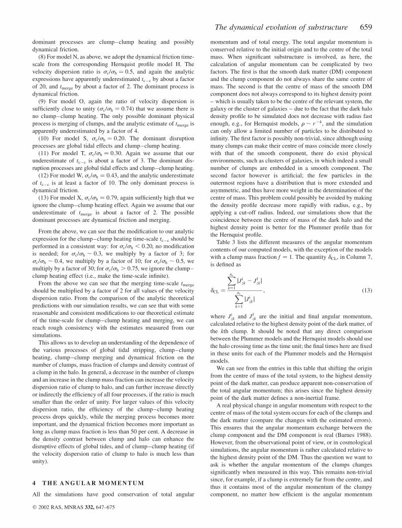
Table 3 lists the different measures of the angular momentum

contents of our computed models, with the exception of the models

with a clump mass fraction f ¼ 1. The quantity dCL, in Column 7,

is defined as

dCL ¼

Xnc

k¼1

jJizk 2 Jf

zkjXnc

k¼1

jJizkj

; ð13Þ

where Jizk and Jf

zk are the initial and final angular momentum,

calculated relative to the highest density point of the dark matter, of

the kth clump. It should be noted that any direct comparison

between the Plummer models and the Hernquist models should use

the halo crossing time as the time unit; the final times here are fixed

in these units for each of the Plummer models and the Hernquist

models.

We can see from the entries in this table that shifting the origin

from the centre of mass of the total system, to the highest density

point of the dark matter, can produce apparent non-conservation of

the total angular momentum; this arises since the highest density

point of the dark matter defines a non-inertial frame.

A real physical change in angular momentum with respect to the

centre of mass of the total system occurs for each of the clumps and

the dark matter (compare the changes with the estimated errors).

This ensures that the angular momentum exchange between the

clump component and the DM component is real (Barnes 1988).

However, from the observational point of view, or in cosmological

simulations, the angular momentum is rather calculated relative to

the highest density point of the DM. Thus the question we want to

ask is whether the angular momentum of the clumps changes

significantly when measured in this way. This remains non-trivial

since, for example, if a clump is extremely far from the centre, and

thus it contains most of the angular momentum of the clumpy

component, no matter how efficient is the angular momentum

The dynamical evolution of substructure 659

q 2002 RAS, MNRAS 332, 647–675

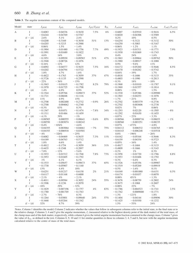
Table 3. The angular momentum content of the computed models.

Model state JrTOT JrCL Jr DM JrCL=JrTOT dCL JcmTOT JcmCL Jcm DM JcmCL=JcmTOT

A I 20.6083 20.04536 20.5630 7.5% 6% 20.6007 20.03910 20.5616 6.5%f 20.6244 20.04769 20.5767 20.6020 20.04306 20.5589

(f 2 i)/i 2.6% 5.1% 2.4% 0.2% 10% 0.5%B I 20.6200 20.3169 20.3030 51% 13% 20.6254 20.3121 20.3132 50%

f 20.6203 20.3215 20.2988 20.6250 20.3083 20.3167(f 2 i)/i 0.06% 1.5% 21.4% 20.06% 21.2% 1.1%

D I 20.1904 20.01480 20.1756 7.7% 49% 20.1923 20.01511 20.1771 7.9%f 20.1991 20.01689 20.1822 20.1930 20.01869 20.1743

(f 2 i)/i 4.6% 14% 3.8% 0.4% 24% 21.6%E I 20.1951 20.09930 20.09583 51% 47% 20.1963 20.09864 20.09762 50%

f 20.1948 20.08726 20.1076 20.1980 20.08917 20.1088(f 2 i)/i 20.16% 212% 12% 0.9% 29.6% 11%

G I 20.6092 20.04577 20.5635 7.5% 16% 20.6172 20.05260 20.5646 8.5%f 20.6202 20.04794 20.5722 20.6170 20.04282 20.5742

(f 2 i)/i 1.8% 4.7% 1.6% 20.04% 219% 1.7%H I 20.4822 20.1763 20.3059 37% 47% 20.4818 20.1686 20.3133 35%

f 20.3726 20.1135 20.2590 20.4803 20.1990 20.2813(f 2 i)/i 222% 236% 215% 20.3% 18% 210%

J I 20.1943 20.01615 20.1782 8.2% 79% 20.1968 20.01810 20.1787 9.1%f 20.1970 20.01725 20.1798 20.1969 20.01557 20.1814

(f 2 i)/i 1.4% 6.9% 0.9% 0.08% 213% 1.5%K I 20.1544 20.05766 20.09673 37% 52% 20.1530 20.05386 20.09900 35%

f 20.1721 20.06048 20.1116 20.1503 20.04253 20.1078(f 2 i)/i 11% 4.9% 15% 21.7% 221% 8.8%

M I 20.2708 0.002488 20.2732 20.9% 26% 20.2702 0.003379 20.2736 21%f 20.2700 0.004062 20.2740 20.2702 0.003606 20.2738

(f 2 i)/i 20.3% 63% 0.3% 0.02% 7% 0.06%N I 20.1367 0.01071 20.1474 27.8% 34% 20.1293 0.02120 20.1505 28%

f 20.1311 0.01484 20.1459 20.1292 0.01630 20.1455(f 2 i)/i 24.1% 39% 21% 20.07% 223% 23.3%

P I 20.08585 0.000555 20.08641 20.6% 85% 20.08566 0.0008716 20.08653 21%f 20.08550 20.003074 20.08242 20.08560 20.003251 20.08235

(f 2 i)/i 20.4% 2654% 24.6% 20.07% 2473% 24.8%Q I 20.04355 0.003064 20.04661 27% 75% 20.04112 0.006532 20.04765 216%

f 20.04193 20.006918 20.03501 20.04143 20.006248 20.03518(f 2 i)/i 24% 2326% 225% 0.8% 2196% 226%

S I 20.6082 20.04469 20.5635 7.3% 11% 20.6162 20.05164 20.5646 8.3%f 20.6189 20.04763 20.5712 20.6159 20.04354 20.5723

(f 2 i)/i 1.8% 6.6% 1.4% 20.05% 216% 1.4%T I 20.4812 20.1754 20.3059 36% 31% 20.4817 20.1684 20.3133 35%

f 20.4435 20.1548 20.2897 20.4809 20.1666 20.3143(f 2 i)/i 27.8% 212% 25.6% 20.2% 1% 0.3%

U I 20.1933 20.01512 20.1768 7.8% 73% 20.1958 20.01720 20.1786 8.8%f 20.1953 20.01605 20.1792 20.1953 20.01606 20.1792

(f 2 i)/i 1% 6.1% 6.1% 20.3% 26.6% 0.3%V I 20.1533 20.05657 20.09673 37% 65% 20.1526 20.05356 20.09907 35%

f 20.1730 20.05907 20.1140 20.1519 20.05269 20.09919(f 2 i)/i 13% 4.4% 18% 20.5% 21.6% 0.1%

W I 20.6251 20.01217 20.6130 2% 21% 20.6169 20.001880 20.6151 0.3%f 20.6117 20.01168 20.6000 20.6174 20.01037 20.6070

(f 2 i)/i 22.1% 24% 22.1% 0.08% 451% 21.3%X I 20.4011 20.09584 20.3052 24% 55% 20.3678 20.08759 20.2802 24%

f 20.3306 20.1236 20.2070 20.3675 20.1068 20.2607(f 2 i)/i 218% 29% 232% 20.08% 22% 27%

Y I 20.1829 20.007196 20.1757 4% 83% 20.1786 20.004523 20.1741 2.5%f 20.1780 20.001705 20.1763 20.1762 0.0009680 20.1771

(f 2 i)/i 22.7% 276% 0.3% 21.3% 2121% 1.8%Z I 20.1264 20.03001 20.09640 24% 57% 20.1404 20.04144 20.09896 30%

f 20.1668 20.03264 20.1342 20.1425 20.01930 20.1232(f 2 i)/i 32% 8.7% 39% 1.5% 253% 24%

Notes. Column 1 identifies the model; Column 2 indicates whether the values that follow in subsequent columns refer to the initial state, to the final state or tothe relative change. Columns 3, 4 and 5 give the angular momentum, Jz (measured relative to the highest density point of the dark matter) of the total mass, ofthe clump mass and of the dark matter, respectively, while column 6 gives the initial angular momentum fraction contained in the clumpy mass. Column 7 givesthe value of dCL, as defined in the text. Columns 8, 9, 10 and 11 list similar quantities to those in columns 3, 4, 5 and 6, but now with the angular momentumcalculated relative to the centre of mass of the total mass.

660 B. Zhang et al.

q 2002 RAS, MNRAS 332, 647–675

transfer from the remaining clumps to the dark matter, the angular

momentum change of the total clump system will be very small.

Thus we must address not only the total angular momentum change

of the clumps, but also the angular momentum change of each

individual clump.

The parameter dCL is useful in quantifying the mean angular

momentum change of an individual clump. Figs 9 and 10 show the

binding energy and angular momentum for each individual clump.

It should be noted that in our simulations in which the smooth (dark

matter) component has a Plummer profile, the initial direction of

the angular momentum vector of the clumpy component is in the

opposite direction to that of the DM component. This is simply a

result of the random assignment of the initial velocity, leading to

negative values of the angular momentum for (several of) the

clumps at large radius. From the plots of models M and P (Figs 9

and 10 respectively) we can see that this fluctuation leads to a lower

initial specific angular momentum than in the Hernquist models.

Thus the total angular momentum of the clumps can be changed

drastically compared to its initial value, even if the change of

angular momentum of an individual clump is slight. Thus we

conclude that dCL is a more robust parameter to measure changes in

angular momentum than is the percentage change of the total

angular momentum of the clumps, especially for the Plummer

models.

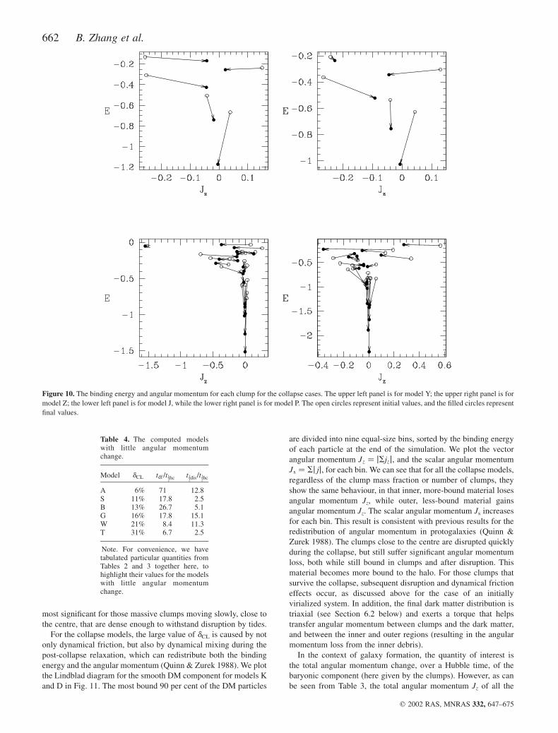
From the entries in Table 3 we can see that dCL for all the

collapse models is much larger than most of the virialized models.

By checking individual clumps, as illustrated in Figs 9 and 10, we

find that clumps close to the centre have significant angular

momentum loss, while the clumps at large distance can have

significant angular momentum change – gains and losses – in

collapse cases.

For the virialized models A, S, B, G, W and T, dCL is small, while

for the remaining virialized models dCL is large. We list the

dynamical friction time and the time for half of the mass in clumps

to be disrupted, in units of t12hc, for these models, in increasing order

of the value of dCL, in Table 4. We can see that there are two factors

that determine the angular momentum change dCL: the dynamical

friction time and the disruption time. Generally, long dynamical

friction times and short disruption times produce small values of

dCL. As discussed in Section 3.1.4, dynamical friction acts to drive

clumps to the centre, with loss of angular momentum of the

clumps. On the other hand, efficient disruption of a clump,

especially due to processes unrelated to dynamical friction such as

clump–clump heating or global tidal effects, helps to decrease the

mass of the clump, which slows down the dynamical friction

process, and thus can decrease the angular momentum loss. In the

extreme case, a clump will no longer suffer dynamical friction after

being disrupted completely. Thus the angular momentum change is

Figure 9. The binding energy and angular momentum for each clump for the virialized cases. The upper left panel is for model W; the upper right panel is for

model X; the lower left panel is for model G, while the lower right panel is for model M. The open circles represent initial values, and the filled circles represent

final values.

The dynamical evolution of substructure 661

q 2002 RAS, MNRAS 332, 647–675

most significant for those massive clumps moving slowly, close to

the centre, that are dense enough to withstand disruption by tides.

For the collapse models, the large value of dCL is caused by not

only dynamical friction, but also by dynamical mixing during the

post-collapse relaxation, which can redistribute both the binding

energy and the angular momentum (Quinn & Zurek 1988). We plot

the Lindblad diagram for the smooth DM component for models K

and D in Fig. 11. The most bound 90 per cent of the DM particles

are divided into nine equal-size bins, sorted by the binding energy

of each particle at the end of the simulation. We plot the vector

angular momentum Jz ¼ jSjzj, and the scalar angular momentum

Js ¼ Sj jj, for each bin. We can see that for all the collapse models,

regardless of the clump mass fraction or number of clumps, they

show the same behaviour, in that inner, more-bound material loses

angular momentum Jz, while outer, less-bound material gains

angular momentum Jz. The scalar angular momentum Js increases

for each bin. This result is consistent with previous results for the

redistribution of angular momentum in protogalaxies (Quinn &

Zurek 1988). The clumps close to the centre are disrupted quickly

during the collapse, but still suffer significant angular momentum

loss, both while still bound in clumps and after disruption. This

material becomes more bound to the halo. For those clumps that

survive the collapse, subsequent disruption and dynamical friction

effects occur, as discussed above for the case of an initially

virialized system. In addition, the final dark matter distribution is

triaxial (see Section 6.2 below) and exerts a torque that helps

transfer angular momentum between clumps and the dark matter,

and between the inner and outer regions (resulting in the angular

momentum loss from the inner debris).

In the context of galaxy formation, the quantity of interest is

the total angular momentum change, over a Hubble time, of the

baryonic component (here given by the clumps). However, as can

be seen from Table 3, the total angular momentum Jz of all the

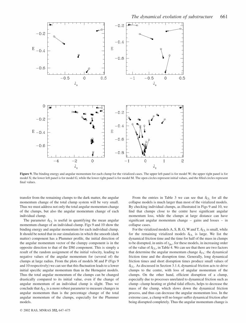
Figure 10. The binding energy and angular momentum for each clump for the collapse cases. The upper left panel is for model Y; the upper right panel is for

model Z; the lower left panel is for model J, while the lower right panel is for model P. The open circles represent initial values, and the filled circles represent

final values.

Table 4. The computed modelswith little angular momentumchange.

Model dCL tdf /t12hc t1

2dis/t1

2hc

A 6% 71 12.8S 11% 17.8 2.5B 13% 26.7 5.1G 16% 17.8 15.1W 21% 8.4 11.3T 31% 6.7 2.5

Note. For convenience, we havetabulated particular quantities fromTables 2 and 3 together here, tohighlight their values for the modelswith little angular momentumchange.

662 B. Zhang et al.

q 2002 RAS, MNRAS 332, 647–675

clumps does not change as much as would be expected from the

parameter dCL, except for model Y and all the Plummer models.

For the Plummer models, as we discussed above, the large change

in the total angular momentum of the clumpy component is due to

the particular random choice of the initial (low) specific angular

momentum of this component. As an upper limit, we may adopt the

parameter dCL as the estimate of the angular momentum change for

the clump system. Our simulations show that the total angular

momentum of the clumpy component does not change significantly

in a Hubble time for a small clump mass fraction and a large

number of clumps, but does change significantly (quantified by dCL

in Table 3 being greater than ,30 per cent) in models with few and

massive clumps; compare model G with model H, or model S with

model T, or model B with model X. Such a high amplitude of

angular momentum loss from protodisc material cannot allow a

spiral to form that matches observation. Thus we conclude that

spiral galaxies can be formed through the accretion of many, but

small, clumps, that conserve angular momentum in the process,

but cannot be formed in an environment that contains only a few,

but large, clumps (cf. Silk & Wyse 1993).

5 T H E K I N E M AT I C S

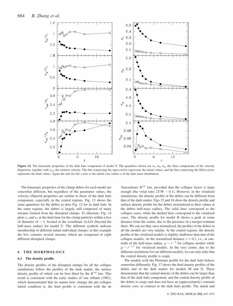
In all of the collapse models the kinematic properties for the dark

halo component are similar, regardless of the different parameter

values. From Fig. 12, we can see that after collapse the radial

velocity dispersion sr increases at all radii, but the increase is

larger in the central regions than at large radius. The other

components of the velocity dispersion tensor, sf and su, increase

less than does sr, with sf slightly larger than su, and they do not

increase significantly at large radius. Thus the final ratios su/sr and

sf/sr decrease with increasing radius. However, at the centre, the

velocity ellipsoid approaches isotropy, i.e., su , sf , sr. The

rotation velocity, Vrot, increases, while V rot/sr decreases. V rot/sf

decreases during the collapse in the central regions, but is fairly

constant in time at large radius.

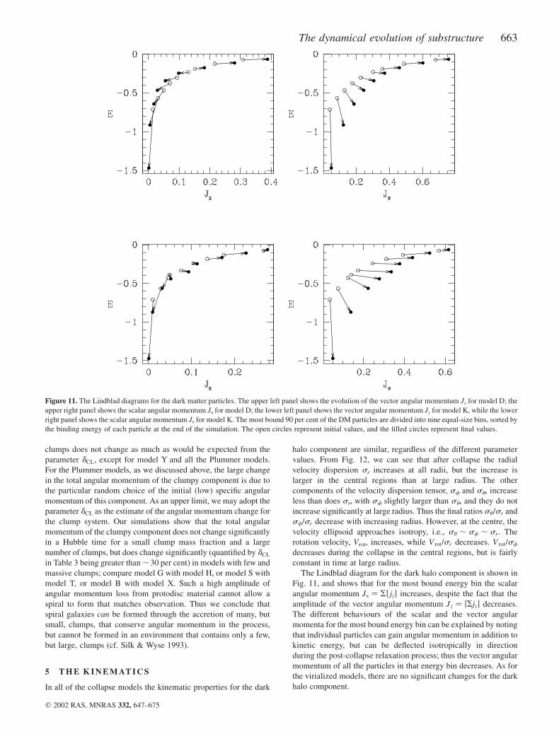
The Lindblad diagram for the dark halo component is shown in

Fig. 11, and shows that for the most bound energy bin the scalar

angular momentum Js ¼ Sj jzj increases, despite the fact that the

amplitude of the vector angular momentum Jz ¼ jSjzj decreases.

The different behaviours of the scalar and the vector angular

momenta for the most bound energy bin can be explained by noting

that individual particles can gain angular momentum in addition to

kinetic energy, but can be deflected isotropically in direction

during the post-collapse relaxation process; thus the vector angular

momentum of all the particles in that energy bin decreases. As for

the virialized models, there are no significant changes for the dark

halo component.

Figure 11. The Lindblad diagrams for the dark matter particles. The upper left panel shows the evolution of the vector angular momentum Jz for model D; the

upper right panel shows the scalar angular momentum Js for model D; the lower left panel shows the vector angular momentum Jz for model K, while the lower

right panel shows the scalar angular momentum Js for model K. The most bound 90 per cent of the DM particles are divided into nine equal-size bins, sorted by

the binding energy of each particle at the end of the simulation. The open circles represent initial values, and the filled circles represent final values.

The dynamical evolution of substructure 663

q 2002 RAS, MNRAS 332, 647–675

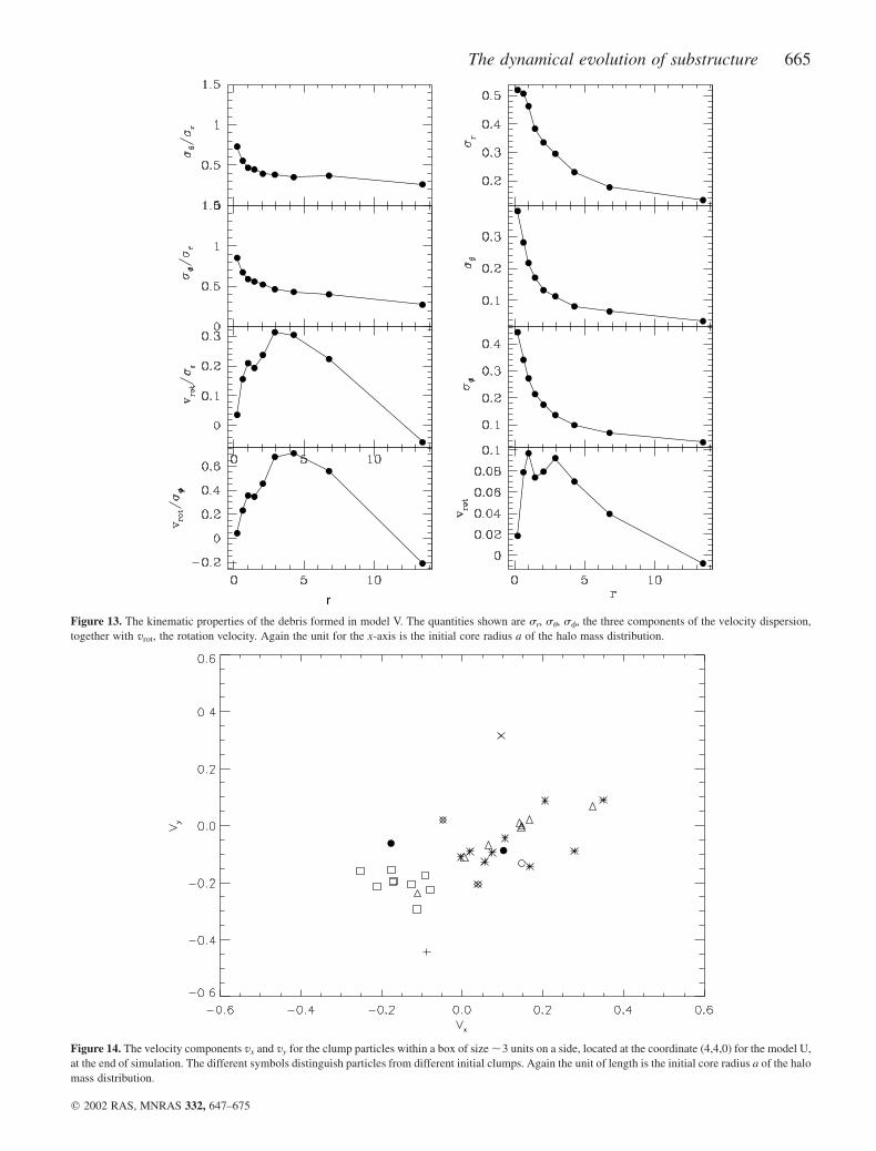
The kinematic properties of the clump debris for each model are

somewhat different, but regardless of the parameter values, the

velocity ellipsoid properties are similar to those of the dark halo

component, especially in the central regions. Fig. 13 shows the

same quantities for the debris as does Fig. 12 for its dark halo. In

the outer regions, the debris is largely still composed of many

streams formed from the disrupted clumps. To illustrate, Fig. 14

plots vx and vy at the final time for the clump particles within a box

of diameter of ,3, located at the coordinate (4,4,0) (beyond the

half-mass radius) for model U. The different symbols indicate

membership of different initial individual clumps; in this example

the box contains several streams, which are composed of eight

different disrupted clumps.

6 T H E M O R P H O L O G Y

6.1 The density profile

The density profiles of the disrupted clumps for all the collapse

simulations follow the profiles of the dark matter, the surface

density profile of which can be best fitted by the R 1=4 law. This

result is consistent with the early studies of van Albada (1982),

which demonstrated that no matter how clumpy the pre-collapse

initial condition is, the final profile is consistent with the de

Vaucouleurs R 1=4 law, provided that the collapse factor is large

enough (the virial ratio 2T/W , 0:1Þ. However, in the virialized

simulations, the density profile of the debris can be different from

that of the dark matter. Figs 15 and 16 show the density profile and

surface density profile for the debris (normalized to their values at

the debris half-mass radius). The solid lines correspond to the

collapse cases, while the dashed lines correspond to the virialized

cases. The density profile for model H shows a peak at some

distance from the centre, due to the presence of a merger remnant

there. We can see that, once normalized, the profiles of the debris in

all the models are very similar. At the central regions, the density

profile of the virialized models is slightly shallower than that of the

collapse models. At the normalized distance r ¼ 0:1, i.e., at one-

tenth of the half-mass radius, r , r 22 for collapse models while

r , r 21:7 for virialized models. At the very centre, due to the

different resolutions for our different models, we can only infer that

the central density profile is cuspy.

The models with the Plummer profile for the dark halo behave

somewhat differently. Fig. 17 shows the final density profiles of the

debris and of the dark matter for models M and N. These

demonstrate that the central density of the debris can be larger than

that of the dark halo component, and the central density profile of

the debris is cuspy and does not have an (approximately) constant

density core, in contrast to the dark halo profile. The initial and

Figure 12. The kinematic properties of the dark halo component of model V. The quantities shown are sr, su, sf, the three components of the velocity

dispersion, together with vrot, the rotation velocity. The line connecting the open circles represents the initial values, and the line connecting the filled circles

represents the final values. Again the unit for the x-axis is the initial core radius a of the halo mass distribution.

664 B. Zhang et al.

q 2002 RAS, MNRAS 332, 647–675

r

Figure 13. The kinematic properties of the debris formed in model V. The quantities shown are sr, su, sf, the three components of the velocity dispersion,

together with vrot, the rotation velocity. Again the unit for the x-axis is the initial core radius a of the halo mass distribution.

Figure 14. The velocity components vx and vy for the clump particles within a box of size ,3 units on a side, located at the coordinate (4,4,0) for the model U,

at the end of simulation. The different symbols distinguish particles from different initial clumps. Again the unit of length is the initial core radius a of the halo

mass distribution.

The dynamical evolution of substructure 665

q 2002 RAS, MNRAS 332, 647–675

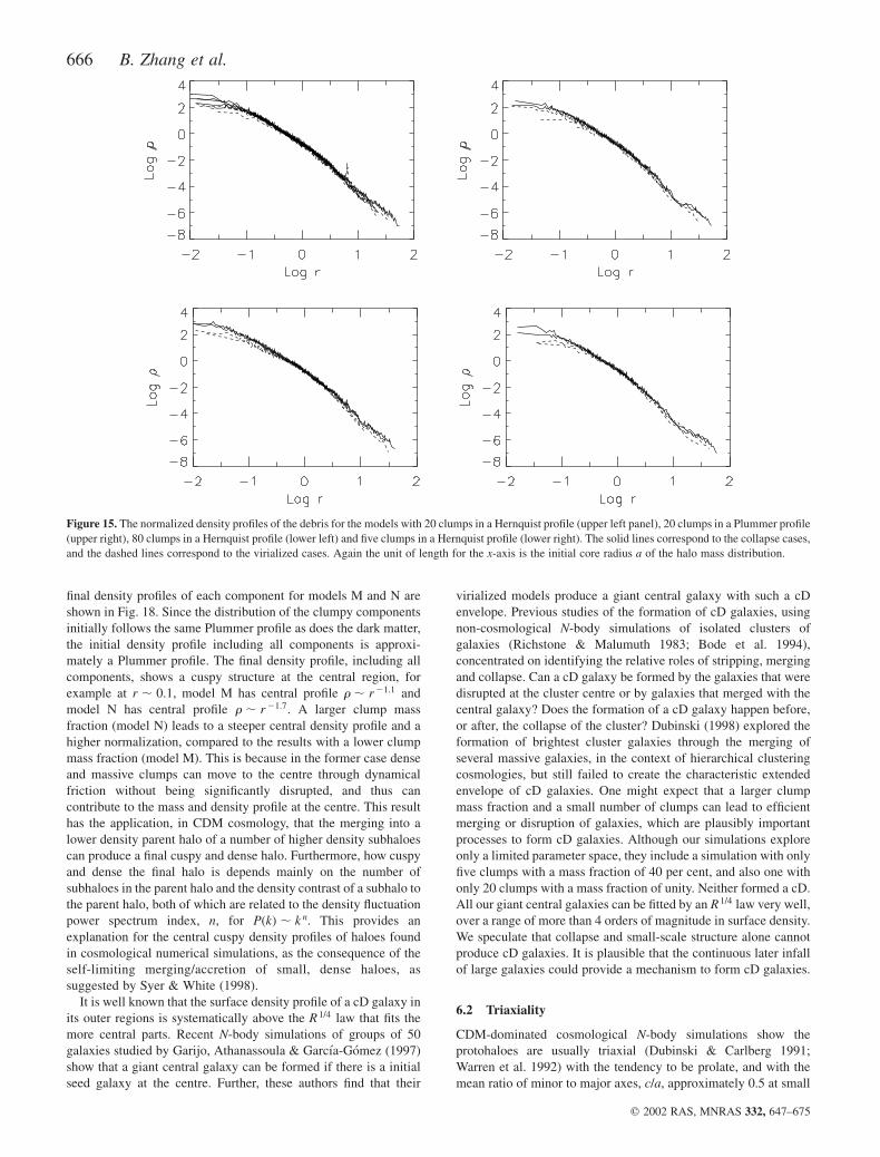
final density profiles of each component for models M and N are

shown in Fig. 18. Since the distribution of the clumpy components

initially follows the same Plummer profile as does the dark matter,

the initial density profile including all components is approxi-

mately a Plummer profile. The final density profile, including all

components, shows a cuspy structure at the central region, for

example at r , 0:1, model M has central profile r , r 21:1 and

model N has central profile r , r 21:7. A larger clump mass

fraction (model N) leads to a steeper central density profile and a

higher normalization, compared to the results with a lower clump

mass fraction (model M). This is because in the former case dense

and massive clumps can move to the centre through dynamical

friction without being significantly disrupted, and thus can

contribute to the mass and density profile at the centre. This result

has the application, in CDM cosmology, that the merging into a

lower density parent halo of a number of higher density subhaloes

can produce a final cuspy and dense halo. Furthermore, how cuspy

and dense the final halo is depends mainly on the number of

subhaloes in the parent halo and the density contrast of a subhalo to

the parent halo, both of which are related to the density fluctuation

power spectrum index, n, for PðkÞ , k n. This provides an

explanation for the central cuspy density profiles of haloes found

in cosmological numerical simulations, as the consequence of the

self-limiting merging/accretion of small, dense haloes, as

suggested by Syer & White (1998).

It is well known that the surface density profile of a cD galaxy in

its outer regions is systematically above the R 1=4 law that fits the

more central parts. Recent N-body simulations of groups of 50

galaxies studied by Garijo, Athanassoula & Garcıa-Gomez (1997)

show that a giant central galaxy can be formed if there is a initial

seed galaxy at the centre. Further, these authors find that their

virialized models produce a giant central galaxy with such a cD

envelope. Previous studies of the formation of cD galaxies, using

non-cosmological N-body simulations of isolated clusters of

galaxies (Richstone & Malumuth 1983; Bode et al. 1994),

concentrated on identifying the relative roles of stripping, merging

and collapse. Can a cD galaxy be formed by the galaxies that were

disrupted at the cluster centre or by galaxies that merged with the

central galaxy? Does the formation of a cD galaxy happen before,

or after, the collapse of the cluster? Dubinski (1998) explored the

formation of brightest cluster galaxies through the merging of

several massive galaxies, in the context of hierarchical clustering

cosmologies, but still failed to create the characteristic extended

envelope of cD galaxies. One might expect that a larger clump

mass fraction and a small number of clumps can lead to efficient

merging or disruption of galaxies, which are plausibly important

processes to form cD galaxies. Although our simulations explore

only a limited parameter space, they include a simulation with only

five clumps with a mass fraction of 40 per cent, and also one with

only 20 clumps with a mass fraction of unity. Neither formed a cD.

All our giant central galaxies can be fitted by an R 1=4 law very well,

over a range of more than 4 orders of magnitude in surface density.

We speculate that collapse and small-scale structure alone cannot

produce cD galaxies. It is plausible that the continuous later infall

of large galaxies could provide a mechanism to form cD galaxies.

6.2 Triaxiality

CDM-dominated cosmological N-body simulations show the

protohaloes are usually triaxial (Dubinski & Carlberg 1991;

Warren et al. 1992) with the tendency to be prolate, and with the

mean ratio of minor to major axes, c/a, approximately 0.5 at small

Figure 15. The normalized density profiles of the debris for the models with 20 clumps in a Hernquist profile (upper left panel), 20 clumps in a Plummer profile

(upper right), 80 clumps in a Hernquist profile (lower left) and five clumps in a Hernquist profile (lower right). The solid lines correspond to the collapse cases,

and the dashed lines correspond to the virialized cases. Again the unit of length for the x-axis is the initial core radius a of the halo mass distribution.

666 B. Zhang et al.

q 2002 RAS, MNRAS 332, 647–675

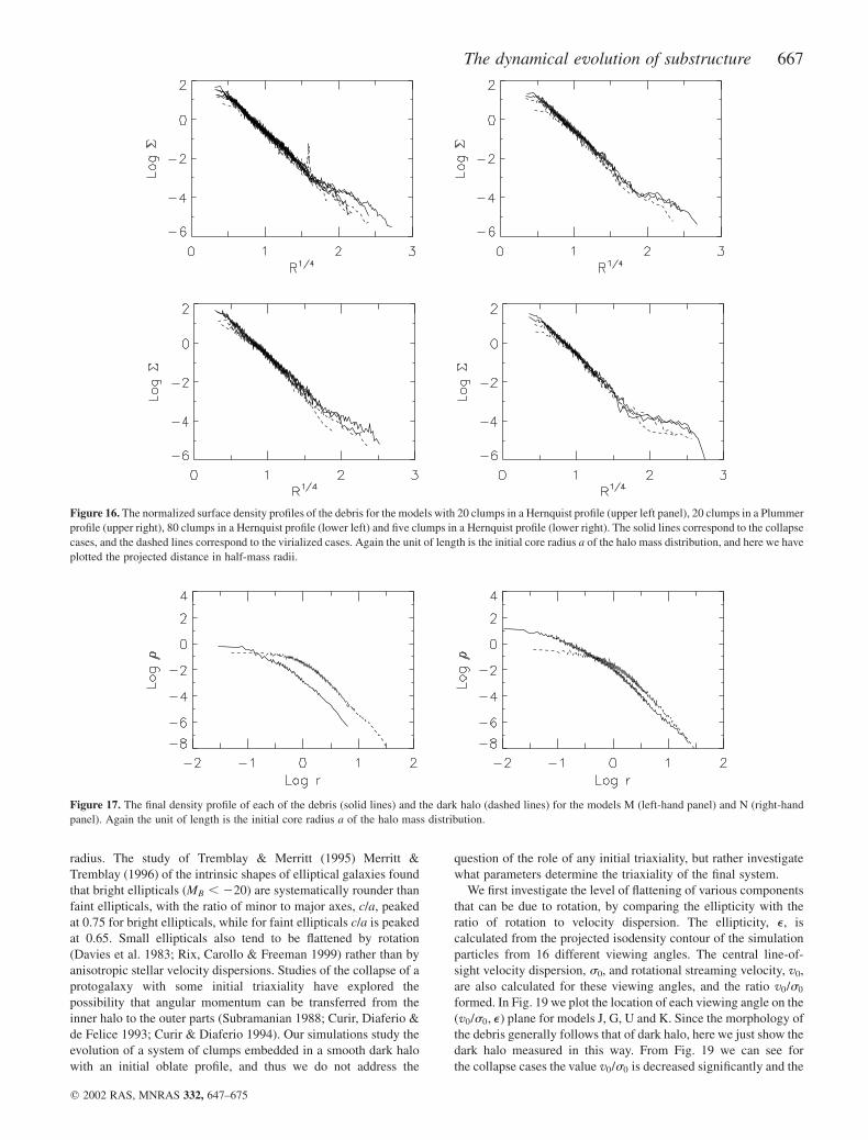
radius. The study of Tremblay & Merritt (1995) Merritt &

Tremblay (1996) of the intrinsic shapes of elliptical galaxies found

that bright ellipticals ðMB , 220Þ are systematically rounder than

faint ellipticals, with the ratio of minor to major axes, c/a, peaked

at 0.75 for bright ellipticals, while for faint ellipticals c/a is peaked

at 0.65. Small ellipticals also tend to be flattened by rotation

(Davies et al. 1983; Rix, Carollo & Freeman 1999) rather than by

anisotropic stellar velocity dispersions. Studies of the collapse of a

protogalaxy with some initial triaxiality have explored the

possibility that angular momentum can be transferred from the

inner halo to the outer parts (Subramanian 1988; Curir, Diaferio &

de Felice 1993; Curir & Diaferio 1994). Our simulations study the

evolution of a system of clumps embedded in a smooth dark halo

with an initial oblate profile, and thus we do not address the

question of the role of any initial triaxiality, but rather investigate

what parameters determine the triaxiality of the final system.

We first investigate the level of flattening of various components

that can be due to rotation, by comparing the ellipticity with the

ratio of rotation to velocity dispersion. The ellipticity, e, is

calculated from the projected isodensity contour of the simulation

particles from 16 different viewing angles. The central line-of-

sight velocity dispersion, s0, and rotational streaming velocity, v0,

are also calculated for these viewing angles, and the ratio v0/s0

formed. In Fig. 19 we plot the location of each viewing angle on the

ðv0/s0; eÞ plane for models J, G, U and K. Since the morphology of

the debris generally follows that of dark halo, here we just show the

dark halo measured in this way. From Fig. 19 we can see for

the collapse cases the value v0/s0 is decreased significantly and the

Figure 16. The normalized surface density profiles of the debris for the models with 20 clumps in a Hernquist profile (upper left panel), 20 clumps in a Plummer

profile (upper right), 80 clumps in a Hernquist profile (lower left) and five clumps in a Hernquist profile (lower right). The solid lines correspond to the collapse

cases, and the dashed lines correspond to the virialized cases. Again the unit of length is the initial core radius a of the halo mass distribution, and here we have

plotted the projected distance in half-mass radii.

Figure 17. The final density profile of each of the debris (solid lines) and the dark halo (dashed lines) for the models M (left-hand panel) and N (right-hand

panel). Again the unit of length is the initial core radius a of the halo mass distribution.

The dynamical evolution of substructure 667

q 2002 RAS, MNRAS 332, 647–675

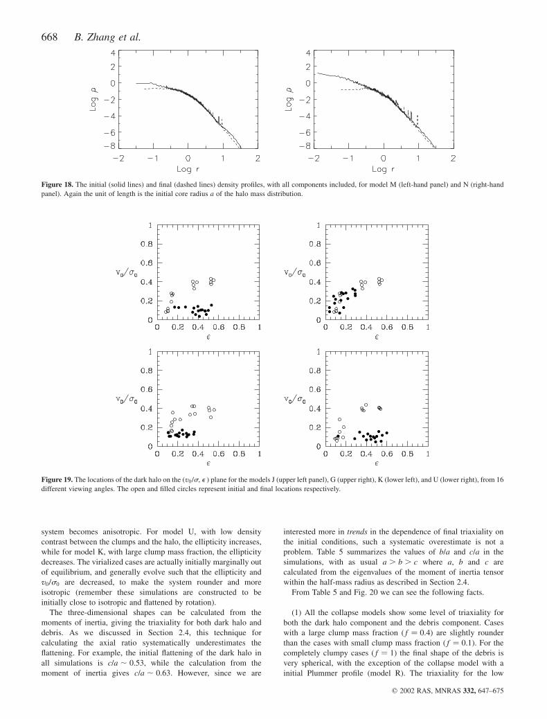
system becomes anisotropic. For model U, with low density

contrast between the clumps and the halo, the ellipticity increases,

while for model K, with large clump mass fraction, the ellipticity

decreases. The virialized cases are actually initially marginally out

of equilibrium, and generally evolve such that the ellipticity and

v0/s0 are decreased, to make the system rounder and more

isotropic (remember these simulations are constructed to be

initially close to isotropic and flattened by rotation).

The three-dimensional shapes can be calculated from the

moments of inertia, giving the triaxiality for both dark halo and

debris. As we discussed in Section 2.4, this technique for

calculating the axial ratio systematically underestimates the

flattening. For example, the initial flattening of the dark halo in

all simulations is c/a , 0:53, while the calculation from the

moment of inertia gives c/a , 0:63. However, since we are

interested more in trends in the dependence of final triaxiality on

the initial conditions, such a systematic overestimate is not a

problem. Table 5 summarizes the values of b/a and c/a in the

simulations, with as usual a . b . c where a, b and c are

calculated from the eigenvalues of the moment of inertia tensor

within the half-mass radius as described in Section 2.4.

From Table 5 and Fig. 20 we can see the following facts.

(1) All the collapse models show some level of triaxiality for

both the dark halo component and the debris component. Cases

with a large clump mass fraction ð f ¼ 0:4Þ are slightly rounder

than the cases with small clump mass fraction ð f ¼ 0:1Þ. For the

completely clumpy cases ð f ¼ 1Þ the final shape of the debris is

very spherical, with the exception of the collapse model with a

initial Plummer profile (model R). The triaxiality for the low

Figure 18. The initial (solid lines) and final (dashed lines) density profiles, with all components included, for model M (left-hand panel) and N (right-hand

panel). Again the unit of length is the initial core radius a of the halo mass distribution.

Figure 19. The locations of the dark halo on the ðv0/s, e ) plane for the models J (upper left panel), G (upper right), K (lower left), and U (lower right), from 16

different viewing angles. The open and filled circles represent initial and final locations respectively.

668 B. Zhang et al.

q 2002 RAS, MNRAS 332, 647–675

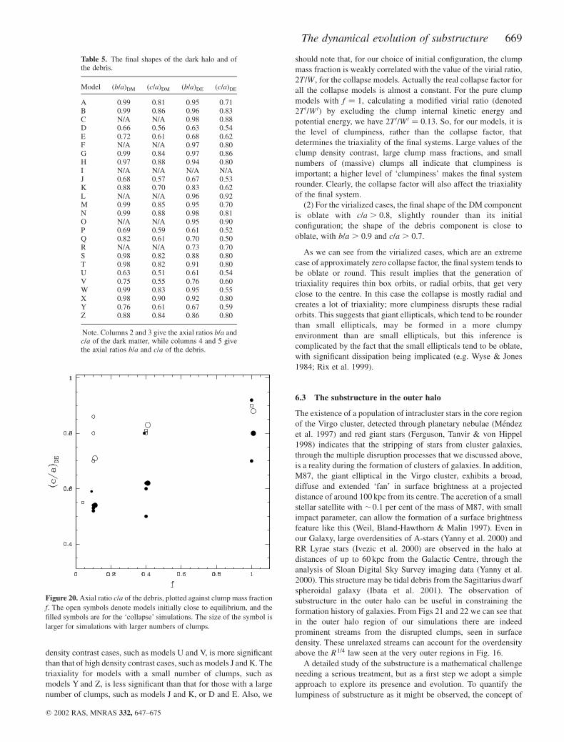
density contrast cases, such as models U and V, is more significant

than that of high density contrast cases, such as models J and K. The

triaxiality for models with a small number of clumps, such as

models Y and Z, is less significant than that for those with a large

number of clumps, such as models J and K, or D and E. Also, we

should note that, for our choice of initial configuration, the clump

mass fraction is weakly correlated with the value of the virial ratio,

2T/W , for the collapse models. Actually the real collapse factor for

all the collapse models is almost a constant. For the pure clump

models with f ¼ 1, calculating a modified virial ratio (denoted

2T 0/W 0Þ by excluding the clump internal kinetic energy and

potential energy, we have 2T 0/W 0 ¼ 0:13. So, for our models, it is

the level of clumpiness, rather than the collapse factor, that

determines the triaxiality of the final systems. Large values of the

clump density contrast, large clump mass fractions, and small

numbers of (massive) clumps all indicate that clumpiness is

important; a higher level of ‘clumpiness’ makes the final system

rounder. Clearly, the collapse factor will also affect the triaxiality

of the final system.

(2) For the virialized cases, the final shape of the DM component

is oblate with c/a . 0:8, slightly rounder than its initial

configuration; the shape of the debris component is close to

oblate, with b/a . 0:9 and c/a . 0:7.

As we can see from the virialized cases, which are an extreme

case of approximately zero collapse factor, the final system tends to

be oblate or round. This result implies that the generation of

triaxiality requires thin box orbits, or radial orbits, that get very

close to the centre. In this case the collapse is mostly radial and

creates a lot of triaxiality; more clumpiness disrupts these radial

orbits. This suggests that giant ellipticals, which tend to be rounder

than small ellipticals, may be formed in a more clumpy

environment than are small ellipticals, but this inference is

complicated by the fact that the small ellipticals tend to be oblate,

with significant dissipation being implicated (e.g. Wyse & Jones

1984; Rix et al. 1999).

6.3 The substructure in the outer halo

The existence of a population of intracluster stars in the core region

of the Virgo cluster, detected through planetary nebulae (Mendez

et al. 1997) and red giant stars (Ferguson, Tanvir & von Hippel

1998) indicates that the stripping of stars from cluster galaxies,

through the multiple disruption processes that we discussed above,

is a reality during the formation of clusters of galaxies. In addition,

M87, the giant elliptical in the Virgo cluster, exhibits a broad,

diffuse and extended ‘fan’ in surface brightness at a projected

distance of around 100 kpc from its centre. The accretion of a small

stellar satellite with ,0.1 per cent of the mass of M87, with small

impact parameter, can allow the formation of a surface brightness

feature like this (Weil, Bland-Hawthorn & Malin 1997). Even in

our Galaxy, large overdensities of A-stars (Yanny et al. 2000) and

RR Lyrae stars (Ivezic et al. 2000) are observed in the halo at

distances of up to 60 kpc from the Galactic Centre, through the

analysis of Sloan Digital Sky Survey imaging data (Yanny et al.

2000). This structure may be tidal debris from the Sagittarius dwarf

spheroidal galaxy (Ibata et al. 2001). The observation of

substructure in the outer halo can be useful in constraining the

formation history of galaxies. From Figs 21 and 22 we can see that

in the outer halo region of our simulations there are indeed

prominent streams from the disrupted clumps, seen in surface

density. These unrelaxed streams can account for the overdensity

above the R 1=4 law seen at the very outer regions in Fig. 16.

A detailed study of the substructure is a mathematical challenge

needing a serious treatment, but as a first step we adopt a simple

approach to explore its presence and evolution. To quantify the

lumpiness of substructure as it might be observed, the concept of

Table 5. The final shapes of the dark halo and ofthe debris.

Model ðb/aÞDM ðc/aÞDM ðb/aÞDE ðc/aÞDE

A 0.99 0.81 0.95 0.71B 0.99 0.86 0.96 0.83C N/A N/A 0.98 0.88D 0.66 0.56 0.63 0.54E 0.72 0.61 0.68 0.62F N/A N/A 0.97 0.80G 0.99 0.84 0.97 0.86H 0.97 0.88 0.94 0.80I N/A N/A N/A N/AJ 0.68 0.57 0.67 0.53K 0.88 0.70 0.83 0.62L N/A N/A 0.96 0.92M 0.99 0.85 0.95 0.70N 0.99 0.88 0.98 0.81O N/A N/A 0.95 0.90P 0.69 0.59 0.61 0.52Q 0.82 0.61 0.70 0.50R N/A N/A 0.73 0.70S 0.98 0.82 0.88 0.80T 0.98 0.82 0.91 0.80U 0.63 0.51 0.61 0.54V 0.75 0.55 0.76 0.60W 0.99 0.83 0.95 0.55X 0.98 0.90 0.92 0.80Y 0.76 0.61 0.67 0.59Z 0.88 0.84 0.86 0.80

Note. Columns 2 and 3 give the axial ratios b/a andc/a of the dark matter, while columns 4 and 5 givethe axial ratios b/a and c/a of the debris.

Figure 20. Axial ratio c/a of the debris, plotted against clump mass fraction

f. The open symbols denote models initially close to equilibrium, and the

filled symbols are for the ‘collapse’ simulations. The size of the symbol is

larger for simulations with larger numbers of clumps.

The dynamical evolution of substructure 669

q 2002 RAS, MNRAS 332, 647–675

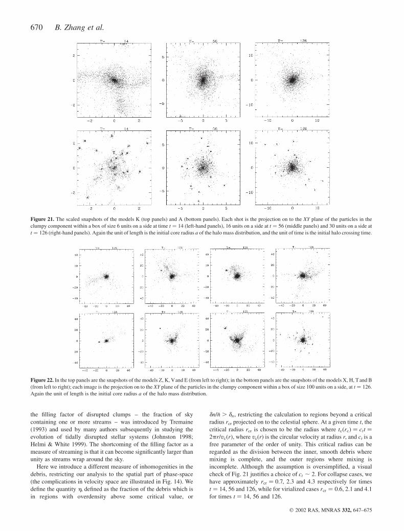
the filling factor of disrupted clumps – the fraction of sky

containing one or more streams – was introduced by Tremaine

(1993) and used by many authors subsequently in studying the

evolution of tidally disrupted stellar systems (Johnston 1998;

Helmi & White 1999). The shortcoming of the filling factor as a

measure of streaming is that it can become significantly larger than

unity as streams wrap around the sky.

Here we introduce a different measure of inhomogenities in the

debris, restricting our analysis to the spatial part of phase-space

(the complications in velocity space are illustrated in Fig. 14). We

define the quantity h, defined as the fraction of the debris which is

in regions with overdensity above some critical value, or

dn/�n . dn, restricting the calculation to regions beyond a critical

radius rcr projected on to the celestial sphere. At a given time t, the

critical radius rcr is chosen to be the radius where tcðrcÞ ¼ ctt ¼

2pr/vcðrÞ; where vc(r) is the circular velocity at radius r, and ct is a

free parameter of the order of unity. This critical radius can be

regarded as the division between the inner, smooth debris where

mixing is complete, and the outer regions where mixing is

incomplete. Although the assumption is oversimplified, a visual

check of Fig. 21 justifies a choice of ct , 2. For collapse cases, we

have approximately rcr ¼ 0:7, 2.3 and 4.3 respectively for times

t ¼ 14, 56 and 126, while for virialized cases rcr ¼ 0:6, 2.1 and 4.1

for times t ¼ 14, 56 and 126.

Figure 22. In the top panels are the snapshots of the models Z, K, Vand E (from left to right); in the bottom panels are the snapshots of the models X, H, T and B

(from left to right); each image is the projection on to the XY plane of the particles in the clumpy component within a box of size 100 units on a side, at t ¼ 126.

Again the unit of length is the initial core radius a of the halo mass distribution.

Figure 21. The scaled snapshots of the models K (top panels) and A (bottom panels). Each shot is the projection on to the XY plane of the particles in the

clumpy component within a box of size 6 units on a side at time t ¼ 14 (left-hand panels), 16 units on a side at t ¼ 56 (middle panels) and 30 units on a side at

t ¼ 126 (right-hand panels). Again the unit of length is the initial core radius a of the halo mass distribution, and the unit of time is the initial halo crossing time.

670 B. Zhang et al.

q 2002 RAS, MNRAS 332, 647–675

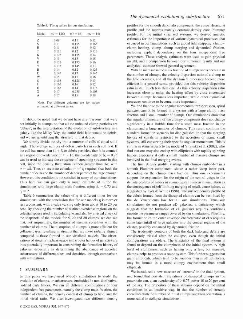
It should be noted that we do not have any ‘baryons’ that were

not initially in clumps, so that all the unbound clump particles are

‘debris’; in the interpretation of the evolution of substructure in a

galaxy like the Milky Way, the entire field halo would be debris,

and we are quantifying the structure in that debris.

We simply divide the sky into a number of cells of equal solid

angle. The average number of debris particles in each cell is n. If

the cell has more than ð1þ dnÞ�n debris particles, then it is counted

as a region of overdensity. If �n , 16, the overdensity of dn ¼ 0:75

can be used to indicate the existence of streaming structure in that

cell, since the density fluctuation is then greater than 3s, with

s ¼ffiffiffi�np

. Thus an accurate calculation of h requires that both the

number of cells and the number of debris particles be large enough.

However, this condition is not satisfied in many of our simulations.

Thus here we can give only a rough estimate of h for the

simulations with large clump mass fraction, using dn ¼ 0:75 and

ct ¼ 2.

Table 6 summarizes the values of h at different times for our

simulations, with the conclusion that for our models h is more or

less a constant, with a value varying only from about 10 to 20 per

cent. By checking the number of distinct overdense regions on the

celestial sphere used in calculating h, and also by a visual check of

the snapshots of the models for 5, 20 and 80 clumps, we can see

that, not surprisingly, the number of streams correlates with the

number of clumps. The disruption of clumps is more efficient for

collapse cases, resulting in streams that are more radially aligned

compared to those formed in our virialized models. The obser-

vations of streams in phase-space in the outer haloes of galaxies are

thus potentially important in constraining the formation history of

galaxies, especially in determining the abundance of accreted

substructure of different sizes and densities, through comparison

with simulations.

7 S U M M A RY

In this paper we have used N-body simulations to study the

evolution of clumps, or substructure, embedded in non-dissipative,

isolated dark haloes. We ran 26 different combinations of four

independent free parameters, namely the clump mass fraction, the

number of clumps, the density contrast of clump to halo, and the

initial virial ratio. We also investigated two different density

profiles for the smooth dark halo component: the cuspy Hernquist

profile and the (approximately) constant-density core Plummer

profile. For the initial virialized systems, we derived analytic

estimates for the importance of various dynamical processes that

occurred in our simulations, such as global tidal stripping, clump–

clump heating, clump–clump merging and dynamical friction,

including explicit dependence on the four independent free

parameters. These analytic estimates were used to gain physical

insight, and a comparison between our numerical results and our

analytical estimate showed general agreement.

With an increase in the mass fraction of clumps and a decrease in

the number of clumps, the velocity dispersion ratio of a clump to

the halo increases, and all the dynamical processes become more

efficient in a general sense, provided that this velocity dispersion

ratio is still much less than one. As this velocity dispersion ratio

increases close to unity, the heating effect by close encounters

between clumps becomes less important, while other dynamical

processes continue to become more important.

We find that due to the angular momentum transport seen, spiral

galaxies cannot be formed in a system with a large clump mass

fraction and a small number of clumps. Our simulations show that

the angular momentum of the clumpy component does not change

significantly in a Hubble time for a small mass fraction in the

clumps and a large number of clumps. This result confirms the

standard formation scenario for disc galaxies, in that the merging

history of spirals is restricted to the accretion of many, small

systems, still conserving their specific angular momentum. This is

similar in some aspects to the model of Vitvitska et al. (2002), who

find that one may also end up with ellipticals with rapidly spinning

haloes, especially if only a small number of massive clumps are

involved in the final merging events.

The final density profile, starting with clumps embedded in a

smooth Plummer component, shows a rather steep inner part,

depending on the clump mass fraction. Thus our experiments

support the explanation for the origin of the central cusps in the

density profiles of haloes in cosmological numerical simulation as

the consequence of self-limiting merging of small, dense haloes, as

suggested by Syer & White (1998). The surface density profile of

the debris formed from the disrupted clumps can be best fitted by

the de Vaucouleurs law for all our simulations. Thus our

simulations do not produce cD galaxies, a deficiency which

suggests that the formation of cD galaxies requires conditions

outside the parameter ranges covered by our simulations. Plausibly,

the formation of the outer envelope characteristic of cDs requires

some later infall of large galaxies into the central regions of the

cluster, possibly enhanced by dynamical friction.

The isodensity contours of both the dark halo and debris are

consistently triaxial after the collapse, even though the initial

configurations are oblate. The triaxiality of the final system is

found to depend on the clumpiness of the initial system. A high

level of clumpiness, such as having only a few, but massive,

clumps, helps to produce a round system. This further suggests that

giant ellipticals, which tend to be rounder than small ellipticals,

may be formed in a more clumpy environment than small

ellipticals.

We introduced a new measure of ‘streams’ in the final system,

and found that persistent signatures of disrupted clumps in the

outer halo can, at an overdensity of .0.75, cover 10 to 20 per cent

of the sky. The properties of these streams depend on the initial

conditions in an intuitive way, in that the number of streams

correlates with the number of initial clumps, and their orientation is

more radial in collapse simulations.

Table 6. The h values for our simulations.

Model hðt ¼ 126Þ hðt ¼ 56Þ hðt ¼ 14Þ

Z 0.08 0.11 0.12S 0.1 0.155 0.165H 0.11 0.13 0.12T 0.115 0.12 0.135K 0.125 0.155 0.14V 0.13 0.13 0.18E 0.135 0.175 0.16Y 0.135 0.145 0.13B 0.14 0.12 0.125U 0.145 0.17 0.145W 0.15 0.17 0.16G 0.155 0.125 0.13J 0.165 0.16 0.12D 0.165 0.14 0.175X 0.17 0.235 0.105A 0.17 0.15 0.18

Note. The different columns are for valuesestimated at different times.

The dynamical evolution of substructure 671

q 2002 RAS, MNRAS 332, 647–675

Some extensions of our work that would further our under-

standing of the role of substructure in the formation of galaxies and

of cluster of galaxies include N-body simulations with (1) a mass

spectrum of clumps rather than identical clumps, (2) less restricted

coverage of parameter space, in particular to larger collapse

factors, and (3) explicit incorporation of a merging criterion into

the calculation at each time-step.

AC K N OW L E D G M E N T S

We acknowledge support from NSF grant AST-9804706 (RFGW)

and the PPARC visitor programme. RFGW thanks all the

Astronomy group at St Andrews for providing a pleasant and

stimulating environment.

R E F E R E N C E S

Aarseth S. J., Fall S. M., 1980, ApJ, 236, 43

Barnes J., 1988, ApJ, 331, 699

Barnes J., Efstathiou G., 1987, ApJ, 319, 575

Barnes J., Hut P., 1986, Nat, 324, 446

Bendo G., Barnes J., 2000, MNRAS, 316, 315

Bertschinger E., Watts P. N., 1988, ApJ, 328, 23

Binney J., Tremaine S., 1987, Galactic Dynamics. Princeton Univ. Press,

Princeton

Bode P. W., Berrington R. C., Cohn H. N., Lugger P., 1994, ApJ, 433, 479

Bontekoe T. R., van Albada T. S., 1987, MNRAS, 224, 349

Brinchmann J., Ellis R. S., 2000, ApJ, 536, L77

Carlberg R. G., 1994, ApJ, 433, 468

Chandrasekhar S., 1943, ApJ, 97, 251

Cole S., Lacey C., 1996, MNRAS, 281, 716

Colpi M., Mayer L., Governato F., 1999, ApJ, 525, 720

Cora S. A., Muzzio J. C., Vergne M. M., 1997, MNRAS, 289, 253

Cretton N., Naab T., Rix H.-W., Burkert A., 2001, ApJ, 554, 291

Curir A., Diaferio A., 1994, A&A, 285, 389

Curir A., Diaferio A., de Felice F., 1993, ApJ, 413, 70

Dalcanton J. J., Spergel D. N., Summers F. J., 1997, ApJ, 482, 659

Davies R., Efstathiou G. P., Fall S. M., Illingworth G., Schechter P., 1983,

ApJ, 266, 41

Domınguez-Tenreiro R., Gomez-Flechoso M. A., 1998, MNRAS, 294, 465

Dressler A., 1984, ARA&A, 22, 185

Dubinski J., 1998, ApJ, 502, 141

Dubinski J., Carlberg R. G., 1991, ApJ, 378, 496

Edvardsson B., Andersen J., Gustafsson B., Lambert D. L., Nissen P. E.,

Tomkin J., 1993, A&A, 275, 101

Efstathiou G., Jones B. J. T., 1979, MNRAS, 186, 133

Evrard A. E., Summers F. J., Davis M., 1994, ApJ, 422, 11

Fall S. M., 1980, in Fall S. M., Lynden-Bell D., eds, The Structure and

Evolution of Normal Galaxies. Cambridge Univ. Press, Cambridge, p. 1

Fall S. M., Efstathiou G., 1980, MNRAS, 193, 189

Fall S. M., Rees M. J., 1977, MNRAS, 181, 37

Ferguson A., Johnson R., 2001, ApJ, 559, L13

Ferguson H. C., Tanvir N. R., von Hippel T., 1998, Nat, 391, 461

Filmore J. A., Goldreich P., 1984, ApJ, 281, 1

Frenk C. S., White S. D. M., Efstathiou G. P., Davis M., 1985, Nat, 317, 595

Garijo A., Athanassoula E., Garcıa-Gomez C., 1997, A&A, 327, 930

Ghigna S., Moore B., Governato F., Lake G., Quinn T., Stadel J., 2000, ApJ,

544, 616

Gunn J. E., 1977, ApJ, 218, 592

Gunn J. E., 1982, in Bruck H. A., Coyne G. V., Longair M. S., eds,

Astrophysical Cosmology. Pontificia Academia Scientiarum, p. 233

Gunn J. E., Gott R., 1972, ApJ, 176, 1

Helmi A., White S. D. M., 1999, MNRAS, 307, 495

Hernquist L., 1987, ApJS, 64, 715

Hernquist L., 1990, ApJ, 356, 359

Hernquist L., Weinberg M. D., 1989, MNRAS, 238, 407

Hoffman Y., Shaham J., 1985, ApJ, 297, 16

Ibata R., Irwin M., Lewis G., Stolte A., 2001, ApJ, 547, L133

Iveciz Z. et al., 2000, AJ, 120, 963

Johnston K. V., 1998, ApJ, 495, 297

Johnston K. V., Hernquist L., Bolte M., 1996, ApJ, 465, 278

Jones B. J. T., Wyse R. F. G., 1983, A&A, 120, 165

King I. R., 1962, AJ, 67, 471

Klypin A. A., Kravtsov A. V., Valenzuela O., Prada F., 1999, ApJ, 522, 82

Kuhn J. R., Miller R. H., 1989, ApJ, 341, L41

Lin D. N. C., Tremaine S., 1983, ApJ, 264, 364

Makino J., Hut P., 1997, ApJ, 481, 83

Maoz E., 1993, MNRAS, 263, 75

Mendez R. H., Guerrero M. A., Freeman K. C., Arnaboldi M., Kudritzki

R. P., Hopp U., Capaccioli M., Ford H., 1997, ApJ, 491, L23

Merritt D., Tremblay B., 1996, AJ, 111, 2243

Mo H. J., Mao S., White S. D. M., 1998, MNRAS, 295, 319

Moore B., Ghigna S., Governato F., Lake G., Quinn T., Stadel J., Tozzi P.,

1999, ApJ, 524, L19

Navarro J. F., Benz W., 1991, ApJ, 380, 320

Navarro J. F., Steinmetz M., 1997, ApJ, 478, 13

Navarro J. F., Frenk C. S., White S. D. M., 1995, MNRAS, 275, 56

Navarro J. F., Frenk C. S., White S. D. M., 1997, ApJ, 490, 493

Peebles P. J. E., 1969, ApJ, 155, 393

Plummer H. C., 1911, MNRAS, 71, 460

Quinn P. J., Zurek W. H., 1988, ApJ, 331, 1

Quinn P. J., Salmon J. K., Zurek W. H., 1986, Nat, 322, 329

Richstone D. O., Malumuth E. M., 1983, ApJ, 268, 3

Rix H.-W., Carollo M., Freeman K. C., 1999, ApJ, 513, L25

Sellwood J. A., 1987, ARA&A, 25, 151

Silk J., 2001, MNRAS, 324, 313

Silk J., Wyse R. F. G., 1993, Physics Reports, 231, 295

Spitzer L., 1987, Dynamical Evolution of Globular Clusters. Princeton

Univ. Press, Princeton

Steinmetz M., Bartelmann M., 1995, MNRAS, 272, 570

Subramanian K., 1988, MNRAS, 234, 459

Syer D., White S. D. M., 1998, MNRAS, 293, 337

Tremaine S., 1981, in Fall S. M., Lynden-Bell D., eds, The Structure and

Evolution of Normal Galaxies. Cambridge Univ. Press, Cambridge,

p. 67

Tremaine S., 1993, in Holt S. S., Verter F., eds, AIP Conf. Proc., Back to the

Galaxy. New York, p. 599

Tremaine S., Weinberg M. D., 1984, MNRAS, 209, 729

Tremblay B., Merritt D., 1995, AJ, 110, 1039

Tsuchiya T., Shimada M., 2000, ApJ, 532, 294

van Albada T. S., 1982, MNRAS, 201, 939

van den Bosch F. C., Geraint F. L., Lake G., Joachim S., 1999, ApJ, 515, 50

van Kampen E., 1995, MNRAS, 273, 295

Vedel H., Hellsten U., Sommer-Larsen J., 1994, MNRAS, 271, 743

Velazquez H., White S. D. M., 1999, MNRAS, 304, 254

Vitvitska M. et al., 2001, ApJ, submitted, astro-ph/0105349

Warren M. S., Quinn P. J., Salmon J. K., Zurek W. H., 1992, ApJ, 399, 405

Weil M. L., Bland-Hawthorn J., Malin D. F., 1997, ApJ, 490, 664

Weil M. L., Eke V. R., Efstathiou G., 1998, MNRAS, 300, 773

Weinberg M. D., 1989, MNRAS, 239, 549

White S. D. M., 1976, MNRAS, 174, 467

White S. D. M., 1978, MNRAS, 184, 185

White S. D. M., 1983, ApJ, 274, 53

White S. D. M., Rees M. J., 1978, MNRAS, 183, 341

Wyse R. F. G., 1999, Baltic Astronomy, 8, 593

Wyse R. F. G., Jones B. J. T., 1984, ApJ, 286, 88

Yanny B. et al., 2000, ApJ, 540, 825

Zaritsky D., White S. D. M., 1988, MNRAS, 235, 289

Zaroubi S., Naim A., Hoffman Y., 1996, ApJ, 457, 50

Zhang B., Wyse R. F. G., 2000, MNRAS, 313, 310

Zurek W. H., Quinn P. J., Salmon J. K., 1988, ApJ, 330, 519

672 B. Zhang et al.

q 2002 RAS, MNRAS 332, 647–675

A P P E N D I X A : PA R A M E T E R S A N D U N I T S O F

T H E S I M U L AT I O N S

The density profile, mass profile, corresponding potential, and the

total potential energy of a Hernquist sphere are:

rðrÞ ¼M

2p

a

rðaþ rÞ3; ðA1Þ

MðrÞ ¼Mr 2

ðr þ aÞ2; ðA2Þ

CðrÞ ¼ 2GM

aþ r; ðA3Þ

F ¼ 2GM 2

6a; ðA4Þ

where a is the core radius.

The density profile, mass profile, corresponding potential and

the total potential energy of a Plummer sphere are:

rðrÞ ¼3M

4pa 31þ

r 2

a 2

� �25=2

; ðA5Þ

MðrÞ ¼Mr 3

ðr 2 þ a 2Þ3=2; ðA6Þ

CðrÞ ¼ 2GMffiffiffiffiffiffiffiffiffiffiffiffiffiffiffiffi

r 2 þ a 2p ; ðA7Þ

F ¼ 23p

32

GM 2

a; ðA8Þ

where a is the core radius.

The half-mass radius for the Hernquist profile is r12¼ ð1þ

ffiffiffi2pÞa,

while for the Plummer profile r12

< 1:3a. The mean crossing time

of the dark halo, given by the ratio of the half-mass radius, r12h, to

the circular velocity at the half-mass radius, v12h, is, for the

Hernquist dark halo, t12hc ¼ r1

2h/v1

2h ¼

ffiffiffi2p

1þffiffiffi2pÿ �

1:5¼ 5:3, while

for the Plummer dark halo t12hc ¼ 2:1. The Hernquist models

are allowed to run for about tsim , 126, i.e., approximately 23

times the mean halo crossing time, while for Plummer models the

simulation is stopped after tsim , 56, i.e., approximately 27 times

the mean halo crossing time. For a typical dark halo of a galaxy, the

mean crossing time is about 0.5 Gyr, for v12h , 200 km s21 and

r12h , 100 kpc. Thus a typical simulation duration of 25 mean

crossing times is approximately a Hubble time. The time-scale for

a dark halo typical of a cluster of galaxies is approximately the

same.

There are some simple and convenient relations among the mean

quantities of a given mass profile. For many reasonable spherical

mass profiles, including both the Plummer and Hernquist spheres,

there is an empirical relation between the half-mass radius r12

and

the virial radius rvi, r12

< 0:8rvi, where the virial radius is defined

by the potential energy jFj ; GM 2

2rvi(Spitzer 1987). In the case of an

isotropic velocity dispersion tensor, we can use the mean one-

dimensional velocity dispersion s, defined by j F2j ; 3

2Ms 2,

instead of the circular velocity at the half-mass radius v12. These are

related by v12¼

ffiffiffiffiffiffiffiffiffiffi6=1:6p

s < 2s.

A P P E N D I X B : N U M E R I C A L E F F E C T S

We first discuss the effects of two-body relaxation, for which the

two bodies can be two particles both from a single clump, or two

particles with one from a clump and the other from the dark halo, or

two particles both from the dark halo. Then we discuss the heating

effect of a clump by dark halo particles.

B1 Two-body relaxation

First, we just consider the case that the clump is isolated, i.e., the

two bodies under consideration are both from a single clump. We

know that the evaporation time-scale is usually 100 times the

relaxation time-scale (Binney & Tremaine 1987) for a given

Maxwellian system; this sets the time-scale over which a clump

could suffer evaporative mass loss if the two-body relaxation time

is too short compared to the simulation time. The two-body

relaxation time in a single clump is (Sellwood 1987)

trelax ,0:14Ncl

ln rc

3rs

� � t12cc;

where the Ncl is the number of particles in a single clump, rs is the

softening-length, and t12cc is the internal crossing time within a

clump. The softening-length in the treecode is set at rs ¼

0:5r12clN

21=3cl ; this relatively large value is chosen to suppress

the unphysical two-body relaxation (White 1978), which otherwise

could occur due to the small number of particles used in each

clump (ranging from 150 to 2400).

In terms of the halo crossing time, this two-body relaxation time

can be written as

trelax ,0:14Ncl

ln rc

3rs

� � t12hcffiffiffiffiffiffiffiffiffiffiffi

rcl/r0

p :

Thus the two-body relaxation time in a single clump is shorter, in

terms of the halo crossing time, for larger values of the density

contrast rcl/r0. This poses a limitation for us in exploring the

parameters for clumps of large density contrast, in addition to

the limitation from the CPU time used, which is determined by the

total number of particles. For our computed models with Ncl ¼ 300

and rcl/r0 ¼ 64, we have trelax , 3:5t12hc. In the worst case, with

Ncl ¼ 150 and rcl/r0 ¼ 64, we have trelax , 2t12hc. Since our

simulation time is about 25t12hc, generally our clumps should

suffer somewhat from two-body relaxation effects, which can

lead to some internal manifestation of collisional behaviour such

as mass segregation (to which we are insensitive since we have

adopted equal-mass particles). However, we do not expect there

to be significant mass loss due to evaporation effects, not only

because the estimated evaporation time-scale is very long

compared to our simulation time, but also due to the fact that

adoption of a softening-length can inhibit evaporation. Further-

more, we are not interested, in this study, in the evolution of the

internal structure of the clump, and thus our chosen parameter

values are acceptable.

Next, we turn to consideration of two-body relaxation in the dark

halo, i.e., the two bodies participating in the two-body relaxation

are both from the dark halo. Similarly to the expressions above, we

have

trelax;h ,0:14Nh

ln rh

3rs

� � t12hc;

where Nh is the number of particles in the dark halo. Typically,

trelax;h , 700t12hc. Thus the two-body relaxation effect in the halo

can be ignored.

In addition to the possible evaporation of clump particles due to

two-body heating between two particles within the same clump,

The dynamical evolution of substructure 673

q 2002 RAS, MNRAS 332, 647–675

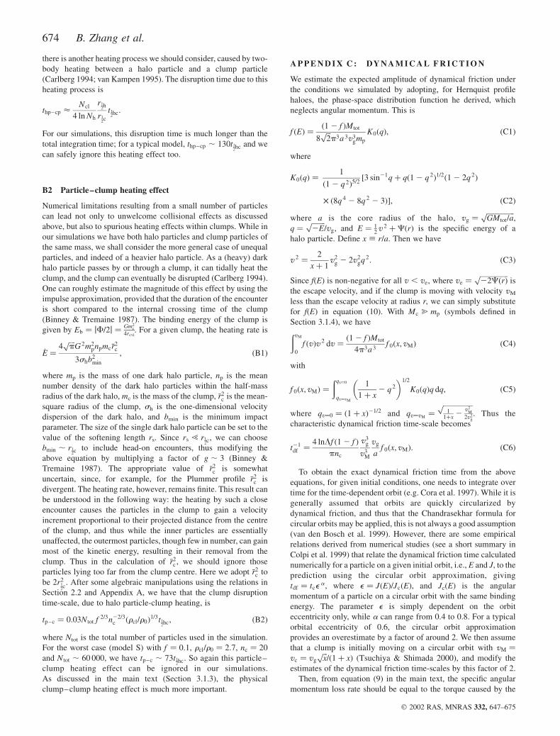
there is another heating process we should consider, caused by two-

body heating between a halo particle and a clump particle

(Carlberg 1994; van Kampen 1995). The disruption time due to this

heating process is

thp–cp <Ncl

4 ln Nh

r12h

r12c

t12hc:

For our simulations, this disruption time is much longer than the

total integration time; for a typical model, thp–cp , 130t12hc and we

can safely ignore this heating effect too.

B2 Particle–clump heating effect

Numerical limitations resulting from a small number of particles

can lead not only to unwelcome collisional effects as discussed

above, but also to spurious heating effects within clumps. While in

our simulations we have both halo particles and clump particles of

the same mass, we shall consider the more general case of unequal

particles, and indeed of a heavier halo particle. As a (heavy) dark

halo particle passes by or through a clump, it can tidally heat the

clump, and the clump can eventually be disrupted (Carlberg 1994).

One can roughly estimate the magnitude of this effect by using the

impulse approximation, provided that the duration of the encounter

is short compared to the internal crossing time of the clump

(Binney & Tremaine 1987). The binding energy of the clump is

given by Eb ¼ jF=2j ¼Gm2

c

4rcvi. For a given clump, the heating rate is

_E ¼4ffiffiffiffipp

G 2m2pnpmc�r

2c

3shb2min

; ðB1Þ

where mp is the mass of one dark halo particle, np is the mean

number density of the dark halo particles within the half-mass

radius of the dark halo, mc is the mass of the clump, �r2c is the mean-

square radius of the clump, sh is the one-dimensional velocity

dispersion of the dark halo, and bmin is the minimum impact

parameter. The size of the single dark halo particle can be set to the

value of the softening length rs. Since rs ! r12c, we can choose

bmin , r12c to include head-on encounters, thus modifying the

above equation by multiplying a factor of g , 3 (Binney &

Tremaine 1987). The appropriate value of �r2c is somewhat

uncertain, since, for example, for the Plummer profile �r2c is

divergent. The heating rate, however, remains finite. This result can

be understood in the following way: the heating by such a close

encounter causes the particles in the clump to gain a velocity

increment proportional to their projected distance from the centre

of the clump, and thus while the inner particles are essentially

unaffected, the outermost particles, though few in number, can gain

most of the kinetic energy, resulting in their removal from the

clump. Thus in the calculation of �r2c , we should ignore those

particles lying too far from the clump centre. Here we adopt �r2c to

be 2r212c

. After some algebraic manipulations using the relations in

Section 2.2 and Appendix A, we have that the clump disruption

time-scale, due to halo particle-clump heating, is

tp–c ¼ 0:03N tot f 2=3n22=3c ðrcl/r0Þ

1=3t12hc; ðB2Þ

where Ntot is the total number of particles used in the simulation.

For the worst case (model S) with f ¼ 0:1, rcl/r0 ¼ 2:7, nc ¼ 20

and N tot , 60 000, we have tp–c , 73t12hc. So again this particle–

clump heating effect can be ignored in our simulations.

As discussed in the main text (Section 3.1.3), the physical

clump–clump heating effect is much more important.

A P P E N D I X C : DY N A M I C A L F R I C T I O N

We estimate the expected amplitude of dynamical friction under

the conditions we simulated by adopting, for Hernquist profile

haloes, the phase-space distribution function he derived, which

neglects angular momentum. This is

f ðEÞ ¼ð1 2 f ÞMtot

8ffiffiffi2p

p3a 3v3gmp

K0ðqÞ; ðC1Þ

where

K0ðqÞ ¼1

ð1 2 q 2Þ5=2½3 sin21qþ qð1 2 q 2Þ1=2ð1 2 2q 2Þ

£ ð8q 4 2 8q 2 2 3Þ�; ðC2Þ

where a is the core radius of the halo, vg ¼ffiffiffiffiffiffiffiffiffiffiffiffiffiffiffiffiGMtot/ap

,

q ¼ffiffiffiffiffiffiffiffi2Ep

/vg, and E ¼ 12

v 2 þCðrÞ is the specific energy of a

halo particle. Define x ; r/a. Then we have

v 2 ¼2

xþ 1v2

g 2 2v2gq 2: ðC3Þ

Since f(E) is non-negative for all v , ve, where ve ¼ffiffiffiffiffiffiffiffiffiffiffiffiffiffiffiffi22CðrÞp

is

the escape velocity, and if the clump is moving with velocity vM

less than the escape velocity at radius r, we can simply substitute

for f(E) in equation (10). With Mc @ mp (symbols defined in

Section 3.1.4), we haveðvM

0

f ðvÞv 2 dv ¼ð1 2 f ÞMtot

4p3a 3f 0ðx; vMÞ ðC4Þ

with

f 0ðx; vMÞ ¼

ðqv¼0

qv¼vM

1

1þ x2 q 2

� �1=2

K0ðqÞq dq; ðC5Þ

where qv¼0 ¼ ð1þ xÞ21=2 and qv¼vM¼

ffiffiffiffiffiffiffiffiffiffiffiffiffiffiffiffiffi1

1þx2

v2M

2v2g

p

. Thus the

characteristic dynamical friction time-scale becomes

t21df ¼

4 lnLf ð1 2 f Þ

pnc

v3g

v3M

vg

af 0ðx; vMÞ: ðC6Þ

To obtain the exact dynamical friction time from the above

equations, for given initial conditions, one needs to integrate over

time for the time-dependent orbit (e.g. Cora et al. 1997). While it is

generally assumed that orbits are quickly circularized by

dynamical friction, and thus that the Chandrasekhar formula for

circular orbits may be applied, this is not always a good assumption

(van den Bosch et al. 1999). However, there are some empirical

relations derived from numerical studies (see a short summary in

Colpi et al. 1999) that relate the dynamical friction time calculated

numerically for a particle on a given initial orbit, i.e., E and J, to the

prediction using the circular orbit approximation, giving

tdf ¼ tcea, where e ¼ JðEÞ/JcðEÞ, and Jc(E) is the angular

momentum of a particle on a circular orbit with the same binding

energy. The parameter e is simply dependent on the orbit

eccentricity only, while a can range from 0.4 to 0.8. For a typical

orbital eccentricity of 0.6, the circular orbit approximation

provides an overestimate by a factor of around 2. We then assume

that a clump is initially moving on a circular orbit with vM ¼

vc ¼ vg

ffiffiffixp

/ð1þ xÞ (Tsuchiya & Shimada 2000), and modify the

estimates of the dynamical friction time-scales by this factor of 2.

Then, from equation (9) in the main text, the specific angular

momentum loss rate should be equal to the torque caused by the

674 B. Zhang et al.

q 2002 RAS, MNRAS 332, 647–675

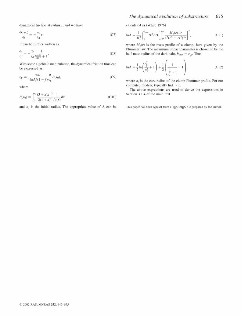
dynamical friction at radius r, and we have

dðrvcÞ

dt¼ 2

vc

tdf

r: ðC7Þ

It can be further written as

dr

dt¼ 2

2r

tdf

1›ln M›ln rþ 1

: ðC8Þ

With some algebraic manipulation, the dynamical friction time can

be expressed as

tdf ¼pnc

4 lnLf ð1 2 f Þ

a

vg

Bðx0Þ; ðC9Þ

where

Bðx0Þ ¼

ðx0

0

ð3þ xÞx 1=2

2ð1þ xÞ41

f 0ðxÞdx; ðC10Þ

and x0 is the initial radius. The appropriate value of L can be

calculated as (White 1976)

lnL ¼1

M2c

ðbmax

0

D 3 dD

ð1

D

McðrÞ dr

r 2ðr 2 2 D 2Þ1=2

� �2

; ðC11Þ

where Mc(r) is the mass profile of a clump, here given by the

Plummer law. The maximum impact parameter is chosen to be the

half-mass radius of the dark halo, bmax ¼ r12h. Thus

lnL ¼1

2ln

r212h

a2c

þ 1

!þ

1

2

1r2

12

h

a2cþ 1

2 1

0BB@1CCA; ðC12Þ

where ac is the core radius of the clump Plummer profile. For our

computed models, typically lnL , 3.

The above expressions are used to derive the expressions in

Section 3.1.4 of the main text.

This paper has been typeset from a TEX/LATEX file prepared by the author.

The dynamical evolution of substructure 675

q 2002 RAS, MNRAS 332, 647–675