THE DOS AND DON·TS OF DISTILLATION COLUMN CONTROL

THE DOS AND DON·TS OF DISTILLATIONCOLUMN CONTROL

S. Skogestad�

Department of Chemical Engineering, Norwegian University of Science and Technology,

Trondheim, Norway.

Abstract: The paper discusses distillation column control within the general framework of plant-wide control. In addition, it aims at providing simple recommendations to assist the engineer indesigning control systems for distillation columns. The standard LV-configuration for level controlcombined with a fast temperature loop is recommended for most columns.

Keywords: configuration selection; temperature location; plantwide control; self-optimizingcontrol; process control; survey.

INTRODUCTION

Distillation control has been extensively studiedover the last 60 years, and most of the dosand don’ts presented in this paper can befound in the existing literature. In particular,the excellent book by Rademaker et al. (1975)contains a lot of useful recommendationsand insights. The problem for the ‘user’ (theengineer) is to find her (or his) way througha bewildering literature (to which I also havemade contributions). Important issues (anddecisions) that need to be addressed by theengineer are related to the following threeproblems:

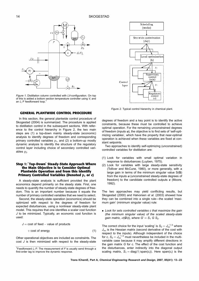
(1) The configuration problem: How shouldpressure and level be controlled, andmore specifically, what is the ‘configur-ation’ defined as the two remainingdegrees of freedom, after having closedthe pressure and level loops? Forexample, should one use the standardLV-configuration (Figure 1), where con-densation flow VT controls pressure p, dis-tillate flow D controls condenser level andbottoms flow B controls reboiler level,such that reflux L and boilup V remainas degrees of freedom for compositioncontrol. Alternatively, should one use a‘material balance’ configuration (DV, LB),a ratio configuration (L/D V; L/D V/B,and so on.)—or maybe even the see-mingly ‘unworkable’ DB-configuration?

(2) The temperature control problem: Shouldone close a temperature loop, and whereshould the temperature sensor be located?

(3) The composition control problem (primarycontrolled variables): Should two, one orno compositions be controlled?

The main objectives of this work are two-fold:

(1) Derive control strategies for distillationcolumns using a systematic procedure.The general procedure for plantwide con-trol of Skogestad (2004) is used here.

(2) From this derive simple recommendationsthat apply to distillation column control.

Is the latter possible? Luyben (2006) has hisdoubts: ‘There are many different types ofdistillation columns and many different typesof control structures. The selection of the“best” control structure is not as simple assome papers claim. Factors that influencethe selection include volatilities, productpurities, reflux ratio, column pressure, costof energy, column size and composition ofthe feed.’Shinskey (1984) made an effort to systema-

tize the configuration problem using thesteady-state RGA. It generated a lot of interestat the time and provides useful insights, butunfortunately the steady-state RGA is gener-ally not a very useful tool for feedback control(e.g., Skogestad and Postlethwaite, 2005).For example, the DB-configuration seemsimpossible from an RGA analysis because ofinfinite steady-state RGA-elements, but it isworkable in practice for dynamic reasons(Finco et al., 1989). The RGA also fails totake into account other important issues,such as disturbances, the overall control objec-tives (economics) and closing of inner loopssuch as for temperature.The paper starts with an overview of the

general procedure for plantwide control, andthen applies it to the three distillation pro-blems introduced above. Simple recommen-dations are given, whenever possible.

13 Vol 85 (A1) 13–23

�Correspondence to:Professor S. Skogestad,Department of ChemicalEngineering, NorwegianUniversity of Science andTechnology, N-7491Trondheim, Norway.E-mail:[email protected]

DOI: 10.1205/cherd06133

0263–8762/07/$30.00þ 0.00

Chemical EngineeringResearch and Design

Trans IChemE,Part A, January 2007

# 2007 Institutionof Chemical Engineers

GENERAL PLANTWIDE CONTROL PROCEDURE

In this section, the general plantwide control procedure ofSkogestad (2004) is summarized. The procedure is appliedto distillation control in the subsequent sections. With refer-ence to the control hierarchy in Figure 2, the two mainsteps are (1) a top-down mainly steady-state (economic)analysis to identify degrees of freedom and correspondingprimary controlled variables y1, and (2) a bottom-up mostlydynamic analysis to identify the structure of the regulatorycontrol layer including choice of secondary controlled vari-ables y2.

Step 1: ‘Top-Down· Steady-State Approach Wherethe Main Objective is to Consider OptimalPlantwide Operation and from this Identify

Primary Controlled Variables (Denoted y1 or c)

A steady-state analysis is sufficient provided the planteconomics depend primarily on the steady state. First, oneneeds to quantify the number of steady-state degrees of free-dom. This is an important number because it equals thenumber of primary controlled variables that we need to select.Second, the steady-state operation (economics) should be

optimized with respect to the degrees of freedom forexpected disturbances, using a nonlinear steady-state plantmodel. This requires that one identifies a scalar cost functionJ to be minimized. Typically, an economic cost function isused:

J ¼ cost of feed� value of products

þ cost of energy (1)

Other operational objectives are included as constraints. Thecost J is then minimized with respect to the steady-state

degrees of freedom and a key point is to identify the activeconstraints, because these must be controlled to achieveoptimal operation. For the remaining unconstrained degreesof freedom (inputs u), the objective is to find sets of ‘self-opti-mizing variables’, which have the property that near-optimaloperation is achieved when these variables are fixed at con-stant setpoints.Two approaches to identify self-optimizing (unconstrained)

controlled variables for distillation are:

(1) Look for variables with small optimal variation inresponse to disturbances (Luyben, 1975).

(2) Look for variables with large steady-state sensitivity(Tolliver and McCune, 1980), or more generally, with alarge gain in terms of the minimum singular value S(G)from the inputs u (unconstrained steady-state degrees offreedom) to the candidate controlled outputs c (Moore,1992).

The two approaches may yield conflicting results, butSkogestad (2000) and Halvorsen et al. (2003) showed howthey can be combined into a single rule—the scaled ‘maxi-mum gain’ (minimum singular value) rule:

. Look for sets controlled variables c that maximize the gain(the minimum singular value) of the scaled steady-stategain matrix, s(G0c=), where G0 ¼ S1 G S2.

The correct choice for the input ‘scaling’ is S2 ¼ Juu21/2 where

Juu is the Hessian matrix (second derivative of the cost withrespect to the inputs). Although independent of the choicefor c, S2 ¼ Juu

21/2 must nevertheless be included in the multi-variable case because it may amplify different directions inthe gain matrix G for c. The effect of the cost function andthe disturbances, enter indirectly into the diagonal outputscaling matrix, S1 ¼ diagf1/span(ci)g. Here span(ci) is the

Figure 1. Distillation column controlled with LV-configuration. On topof this is added a bottom section temperature controller using V, andan L/F feedforward loop.1

Figure 2. Typical control hierarchy in chemical plant.

1Feedforward L/F: The measurement of F is usually send through afirst-order lag to improve the dynamic response.

Trans IChemE, Part A, Chemical Engineering Research and Design, 2007, 85(A1): 13–23

14 SKOGESTAD

expected variation in ci:

Span(ci) ¼ joptimal variation in cij

þ jimplementation error for cij

The optimal variation in ci is due to disturbances d, may beobtained by optimizing for various disturbances using asteady-state model. The steady-state implementation erroris often the same as the measurement error. For example,if we are considering temperatures as candidate controlledvariables, then a typical implementation error is 0.5 C. Inthe scalar case, the minimum singular value is simply thegain jG0j, and here the factor jJuuj does not matter as it willhave the same effect for all choices for c. Therefore, for thescalar case we may rank the alternatives based on maximiz-ing jGj/span(c).Note that only steady-state information is needed for this

analysis and G0 may be obtained, for example, using a com-mercial process simulator. One first needs to find the nominaloptimum, and then make small perturbations in the uncon-strained inputs (to obtain G for the various choices for c),reoptimize for small perturbations in the disturbances d (toobtain the optimal variation that enters in S1), and reoptimizefor small perturbations in u (to obtain Juu that enters in S2).

Step 2: Bottom-Up Identification of a SimpleRegulatory ( ‘Stabilizing·) Control Layer

The main objective of the regulatory layer is to ‘stabilize’the plant. The word ‘stabilize’ is put in quotes, because itdoes not refer to its meaning only in the mathematicalsense, but in the more practical sense of ‘avoiding drift’.More specifically, we here identify ‘extra’ secondary con-trolled variables (denoted y2) and pair these with manipulatedinputs (denoted u2). The main idea is that control of the vari-ables y2 stabilizes the plant and avoids drift. Typical second-ary variables include liquid levels, pressures in key units,some temperatures (e.g., in reactors and distillation columns)and flows. The upper layer uses the setpoints y2s as manipu-lated variables, and when selecting y2 one should also avoidintroducing unnecessary control problems as seen from theupper layer. This results in a hierarchical control structure,with the fastest loop (typically the flow and pressure loops)at the bottom of the hierarchy. The number of possible controlstructures is usually extremely large, so in this part of the pro-cedure one aims at obtaining a good but not necessarily opti-mal structure.Some guidelines for selecting secondary controlled vari-

ables y2 in the regulatory control layer:

(1) The ‘maximum gain rule’ is useful also for selecting y2,but note that the gain should be evaluated at the fre-quency of the layer above. Often the upper layer is rela-tively slow and then a steady-state analysis may besufficient (similar the one used when selecting y1).

(2) Since the regulatory layer is at the bottom of the hierarchyit is important that in does not fail. Therefore, one shouldavoid using ‘unreliable’ measurements.

(3) For dynamic reasons one should avoid variables y2 with alarge (effective) time delay. This, together with the issueof reliability, usually excludes using compositions as sec-ondary controlled variables y2.

(4) To avoid unnecessary cascades and reduce complexity,control primary variables y1 in the regulatory layer (i.e.,choose y2 ¼ y1), provided guidelines 2 and 3 are met.

The selected secondary outputs y2 also need to be ‘paired’with manipulated inputs u2. Some guidelines for selectingu2 in the regulatory control layer:

(1) To avoid failure of the regulatory control layer, avoid vari-ables u2 that may saturate (if one uses a variable thatmay saturate, then it should be monitored and ‘reset’using extra degrees of freedom in the upper controllayer).

(2) Avoid variables u2 where (frequent) changes are undesir-able, for example, because they disturb other parts of theprocess.

(3) Prefer pairing on variables ‘close’ to each other such thatthe effective time delay is small.

Eventually, as loops are closed one also needs to considerthe controllability of the ‘final’ control problem which has theprimary controlled variables y1 ¼ c as outputs and the set-points to the regulatory control layer y2s as inputs. In theend, dynamic simulation may be used to check the proposedcontrol structure, but as it is time consuming and requires adynamic model it should be avoided if possible.We now apply the two-step procedure to distillation, start-

ing with the selection of primary controlled variables (Step 1).

PRIMARY CONTROLLED VARIABLES FORDISTILLATION (STEP 1)

When deriving overall controlled objectives (primary con-trolled objectives) one should generally take a plantwide per-spective and minimize the cost for the overall plant. However,this may be very time consuming, so in practice one usuallyperforms a separate ‘local’ analysis for the distillation col-umns based on internal prices. The cost function (1) for atwo-product distillation column is typically

J ¼ pFF � pDD� pBBþ pQhjQhj þ pQcjQcj

� pFF � pDD� pBBþ pVV(2)

where the (internal, ‘shadow’) prices pi for the feed F and pro-ducts D and B should reflect the plantwide setting. Theapproximation leading to the final expression in (2) appliesbecause typically jQhj � jQcj, and we introduce V ¼ jQhj/cwhere the constant c is the heat of vaporization (J mol21).Then pV ¼ c (pQhþ pQc) represents the cost of heating pluscooling.The cost J in equation (2) should be minimized with respect

to the degrees of freedom, subject to satisfying the oper-ational constraints. Typical constraints for distillation columnsinclude:

Purity top product (D): xD, impurity HK � maxPurity bottom product (B): xB, impurity LK � maxFlow and capacityconstraints:

0 � min F, V, D, B, L,etc, � max

Pressure constraint: min � p � max

To avoid problems with infeasibility or multiple solutions, theimpurity should be in terms of heavy key (HK) componentfor D, and light key (LK) component for B. Many columnsdo not produce final products, and therefore do not have


THE DOS AND DON’TS OF DISTILLATION COLUMN CONTROL 15

purity constraints. However, except for cases where the pro-duct is recycled, there are usually indirect constraintsimposed by product constraints in downstream units, andthese should then be included.In general, a conventional two-product distillation column

has four steady-state degrees of freedom (for example, fee-drate, pressure and two column compositions), but unlessotherwise stated we assume in this paper that feedrate andpressure are given. More specifically, the feedrate isassumed to be a disturbance, and the pressure should becontrolled at a given value. There are then two steady-statedegrees of freedom related to product compositions and wewant to identify two associated controlled variables.

Composition Control

Assume that the feedrate (F) and pressure (p) are given,and that there are purity constraints on both products.Should the two degrees of freedom be used to control bothcompositions (‘two-point control’)?To answer this in a systematic way, we need to consider

the solution to the optimization problem. In general, we findby minimizing the cost J in (2) that the purity constraint forthe most valuable product is always active. The reason isthat we should produce as much as possible as the valuableproduct, or in other words, we should avoid product ‘give-away’. For example, consider separation of methanol andwater and assume that the valuable methanol productshould contain maximum 2% water. This constraint is clearlyalways active, because in order to maximize the productionrate we want to put as much water as possible into themethanol product.However, the purity for the less valuable product constraint

is not necessarily active. There are two cases (the term‘energy’ used below includes energy usage both for heatingand cooling):

. Case 1: If energy is ‘expensive’ [pV in (2) sufficiently large]then the purity constraints for the less valuable product isactive because it costs energy to overpurify.

. Case 2: If energy is sufficiently ‘cheap’ (pV sufficientlysmall), then in order to reduce the loss of the valuable pro-duct, it will be optimal to overpurify the less valuable pro-duct (that is, its purity constraint is not active). There arehere again two cases.

. Case 2a (energy moderately cheap): Unconstrained opti-mum where V is increased until the point where there isan optimal balance (trade-off) between the cost ofincreased energy usage (V), and the benefit of increasedyield of the valuable product

. Case 2b (energy very cheap): Constrained optimum whereit is optimal to increase the energy (V) until a capacity con-straint is reached (e.g., V is at its maximum or the columnapproaches flooding).

In general, we should for optimal operation control the activeconstraints. A deviation from an active constraint is denoted‘back-off’ and always has an economic penalty. The controlimplications are:

. Case 1 (‘expensive’ energy): Use ‘two-point’ control withboth products at their purity constraints.

. Case 2a (‘moderately cheap’ energy where capacity con-straint is not reached): The valuable product should be

controlled at its purity constraint and in addition one shouldcontrol a ‘self-optimizing’ variable which, when kept constant,provides a good trade-off between energy costs andincreased yield. In most cases a good self-optimizingvariable is the purity of the less valuable product. Thus,‘two-point’ control is usually a good policy also in this case,but note that the less valuable product is overpurified, so itssetpoint needs to be found by optimization.

. Case 2b (‘cheap’ energy where capacity constraint isreached): Use ‘one-point’ control with the valuable productat its purity constraint and V increased until the columnreaches its capacity constraint. Note that the cheapproduct is overpurified.

In summary, we find that ‘two-point’ control is a good controlpolicy in many cases, but ‘one-point’ control is optimal ifenergy is sufficiently cheap such that one wants to operatewith maximum energy usage.

RemarkThe above discussion on composition control has only con-

cerned itself with minimizing the steady-state cost J. Inaddition, there are dynamic and controllability considerationsand these generally favour overpurifying the products. Thereason is simply that a ‘back-off’ from the purity specificationsmakes composition control simpler. Overpurification gener-ally requires more energy, but for columns with manystages (relative to the required separation) the optimum in Jis usually very flat, so the additional cost may be verysmall. Before deciding on the composition setpoints it istherefore recommended to perform a sensitivity analysis forthe cost J with the product purity as a degree of freedom.

STABILIZING CONTROL LAYER FORDISTILLATION (STEP 2)

With a given feedrate, a standard two-product distillationcolumn has five dynamic control degrees of freedom(manipulated variables; inputs u). These are the followingfive flows:

u ¼ reflux L, boilupV , top product (distillate)D,

bottoms productB, overhead vaporVT

(3)

In practice, V is often manipulated indirectly by the heatinput (Qh), and VT by the cooling (Qc). In terms of stabiliz-ation, we need to stabilize the two integrating modes associ-ated with the liquid levels (masses) in the condenser andreboiler (MD and MB) In addition, for ‘stable’ operation it isgenerally important to have tight control of pressure (p), atleast in the short time scale (Shinskey, 1984).However, even with these three variables (MD, MB, p) con-

trolled, the distillation column remains (practically) unstablewith a slowly drifting composition profile (in fact, this modein some cases even become truly unstable2). To understandthis, one may view the distillation column as a ‘tank’ with lightcomponent in the top part and heavy component in thebottom part. The ‘tank level’ (column profile) needs to be

2We may have instability with the LV-configuration when separatingcomponents with different molecular weights (e.g., methanol and pro-panol), because a constant mass reflux may give an ‘unstable’ molarreflux due to a positive composition feedback (Jacobsen andSkogestad, 1994).


16 SKOGESTAD

controlled in order to avoid that it drifts out of the column,resulting in breakthrough of light component in the top orheavy component in the bottom.To stabilize the column profile we must use feedback con-

trol as feedforward control cannot change the dynamics andwill eventually give drift. A simple measure of the profilelocation is a temperature measurement (T ) inside thecolumn, so a practical solution is to use temperature feed-back. This feedback loop should be fast, because it takes arelatively short time for a disturbance to cause a significantcomposition change at the column ends. As for level control,a simple proportional controller may be used, or a PI-controllerwith a relatively large integral time.In summary, we have found that the following variables

should be controlled in the stabilizing (regulatory) controllayer:

y2 ¼ MD, MB, p, T (4)

One degree of freedom (flow) remains unused after closingthese loops. In addition, the upper layer may manipulatethe four setpoints for y2. However, note that the setpointsfor MD and MB have no steady-state effect. The setpoint forp has some (but generally not a significant) steady-stateeffect, although it is often optimal to minimize p on the longtime scale (at steady-state) in order to improve the relativevolatility (Shinskey, 1984). In general, the setpoint for T hasa quite large steady-state effect on product compositionsand it is usually manipulated by an upper layer compositioncontroller. However, because the upper layer usuallyoperates on a quite long time scale, we generally want toselect a temperature location such that we achieve indirectcomposition control (with a constant temperature setpoint),and this is further discussed later.The selected secondary outputs y2 need to be ‘paired’

with manipulated variables (inputs) u2. In this paper,we assume that pressure is controlled using VT (cooling),although there are other possibilities. The choice ofinputs for the other variables is discussed in more detailbelow:

. Control configuration: Addresses the issue of which inputsu2 to use for level control (or actually, which inputs u1(flows) that remain for control of y1 after the pressure andlevel control loops have been closed).

. Temperature control: Addresses the location of the temp-erature measurement and which input to use for tempera-ture control (or actually, which input (flow) that remains asan ‘unused’ degree of freedom (fixed on a fast time scale)after the temperature loop has been closed).

RemarkThroughout this paper the feedrate F is assumed to be

given (i.e., F is a disturbance). However, for columns that pro-duce ‘on demand’, F is a degree of freedom (input), andinstead D or B becomes a disturbance. How does thischange the analysis below? With given pressure, thenumber of steady-state degrees freedom is till two. If B isgiven (a disturbance) and F is liquid (which it usually is),then one may simply replace B by F; for example, F isfrequently used for reboiler level control. If D is given (a dis-turbance) and F is liquid, then it is not quite as simple,because F cannot take the role of D. Specifically, if F is

liquid then it cannot be used for condenser level control,which leaves L or V as candidates for condenser levelcontrol, and ‘LV ’-style configuration can not be used. Suchcases will require a more detailed analysis.

CONTROL CONFIGURATION (LEVEL CONTROL)

The term control ‘configuration’ for distillation columnsusually refers to the two combinations of the four flows L,V, D and B that remain (unused) as degrees of freedom(inputs) after the level loops have been closed. For example,in Figure 1 we use the two product flows D and B to controlcondenser and reboiler level, respectively, and (before weadd the feedforward block to get L/F and the feedback temp-erature loop), reflux L and boilup V remain as degrees offreedom—this is therefore called the LV-configuration. TheLV-configuration is the most common or ‘conventional’choice. Another common configuration is the DV-configuration,where L rather than D is used to control condenser level.Changing around the level control in the bottom gives the LB-configuration. The DV- and LB-configurations are known as‘material balance configurations’ because the direct handleon D or B directly adjusts the material balance split for thecolumn. Changing around the level control in both ends givesthe DB-configuration with a direct handle on both D and B.This seems unworkable because of the steady-state materialbalance Dþ B ¼ F, but it is actually workable in practice(Finco et al., 1989) for dynamic reasons (Skogestad et al.,1990). Levels may also be controlled such that ratiosremain as degrees of freedom, for example the L/D V- andL/D V/B-configurations.Many books (Shinskey, 1984) and papers, including sev-

eral of my own (e.g., Skogestad and Morari, 1987), havebeen written on the merits of the various configurations, butit is probably safe to say that the importance of the choiceof configuration (level control scheme) has been overempha-sized. The main reason is that the distillation column, evenafter the two level loops (and pressure loop) have beenclosed, is ‘practically unstable’ with a drifting compositionprofile. To avoid this drift, one needs to close one moreloop, typically a relatively fast temperature loop (often fasterthan the level control loops). This fast loop will again influ-ence the level control. Thus, an analysis of the variousconfigurations (level control schemes), without including atemperature or quality loop, is generally of limited usefulness.

Difference Between Control ConfigurationsWithout a Temperature Loop

Although we just stated that it is of limited usefulness, wewill first look at the difference between the various ‘pure’ con-figurations (without a temperature loop). One reason is thatthis problem has been widely studied and discussed in thedistillation literature. Over the years, the distillation expertshave disagreed strongly on what is the ‘best’ configuration.The reason for the controversy is mainly that the variousexperts put varying emphasis on the following possiblyconflicting issues:

(1) Level control by itself (emphasized e.g., by Buckley et al.,1985).



(2) Interaction of level control (in particular the level controltuning) with the remaining composition control problem(Skogestad, 1997).

(3) ‘Self-regulation’ in terms of disturbance rejection(emphasized e.g., by Skogestad and Morari, 1987).

(4) Remaining two-point control problem in terms of steady-state interactions (emphasized e.g., by Shinskey, 1984).

Level controlIf we look at liquid level control by itself, then it is quite

clear that one generally should use the largest flow to con-trol level. The reason is that it is then less likely that the flowwill saturate, which as noted previously should be avoidedin the lower layers of the control hierarchy. For example,consider control of top level (reflux drum) where one issueis whether to use L or D as an input. The ‘largest flow’rule gives that one should use distillate D (the ‘conventionalchoice’) if L/D , 1, and reflux L for higher reflux columnswith L/D . 1.Partly based on this reasoning, Liptak (2006, Chapter 8.19)

recommends for top level control to use D for L/D , 0.5 (lowreflux ratio), and L for L/D . 6 (high reflux ratio). For inter-mediate reflux ratios either L or D may be used. Thus, theLV-configuration is not recommended for L/D . 6. Similararguments apply to the bottom level, that is, the standardscheme with B for bottom level control is not recommendedif V/B is large (.6). However, as discussed in more detailbelow, these recommendations do not apply when a temp-erature loop is included, because of the ‘indirect’ level controlresulting from the temperature loop.

Interaction between level and composition controlIt is generally desirable that level control and column (com-

position) control are decoupled. That is, retuning of a levelcontroller should not affect the remaining control system.This clearly favors the LV-configuration (where D and B areused for level control) because D and B have by themselvesno effect on the rest of the column.For example, assume that L is used for top level control

(e.g., DV-configuration). The remaining flow D in the topcan then affect the column only indirectly through the actionof the level controller which manipulates L. The top level con-troller then has to be tightly tuned to avoid that the responsefrom D to compositions is delayed and depends on the leveltuning. Furthermore, with tight level control, one is not reallymaking use of the level as a ‘buffer’ and one might aswell eliminate the reflux drum. On the other hand, with theLV-configuration (where D is used for top level control), theremaining flow L has a direct effect on the column andthe level control tuning has no (or negligible) effect on thecomposition response for L.

Disturbance rejectionThe LV-configuration generally has poor self-regulation for

disturbances in F, V, L and in feed enthalpy (Skogestad andMorari, 1987). That is, with only the level loops closed usingD and B, the composition response is very sensitive to thesedisturbances. The DV- or LB-configurations generally behavebetter in this respect, because disturbances in V, L and feedenthalpy are kept inside the column and do not affect theexternal flows (because D is constant). The double ratioconfiguration L/D V/B has even better self-regulating

properties, especially for columns with large internal flows(large L/D and V/B). These conclusions are supported bythe relative composition deviations DX computed for variousconfigurations for a wide range of distillation columns (Horiand Skogestad, 2006); for example see the data for‘column A’ given in the left two columns in Table 1.

Remaining composition control problemWith the LV-configuration, the remaining composition pro-

blem is generally interactive and ill-conditioned, especiallyat steady-state and for high-purity columns. This is easilyexplained because an increase in L (with V constant) hasessentially the opposite effect on composition of an increasein V (with L constant). Thus, the two inputs counteract eachother and the process is strongly interactive. This can bequantified by computing the relative gain array (RGA). Thesteady-state RGA (more precisely, its 1,1-element, which pre-ferably should be close to 1) for various configurations for‘column A’ are (Skogestad and Morari, 1987):

L=D� V=B: 3:22, L� B: 0:56, D� V : 0:45,

L=D� V : 5:85, L� V : 35:1, D� B:1

Note that the steady-state RGA is very large for the LV-configuration and that it is infinite for the DB-configuration.This has led many authors (e.g., Shinskey, 1984) to concludethat the DB-configuration is infeasible, but this conclusion isincorrect. Indeed, with a given feed flow, D and B can notbe changed independently at steady-state because of theconstraint Dþ B ¼ F, but it is possible to make independentchanges dynamically because of the holdup in the column.Similarly, the LV-configuration is much less interactive dyna-mically than the large steady-state RGA-value of 35.1 indi-cates. This reason is that an increase in reflux L willimmediately influence the composition in the top of thecolumn, whereas it takes some time (qL; typically a few min-utes) to ‘move down’ the column and influence the bottomcomposition. This can be more clearly seen from a fre-quency-dependent RGA-plot (not shown in this paper),

Table 1. Relative steady-state composition deviation DX ¼ffiffiffiffiffiffiffiffiffiffiffiffiffiffiffiffiffiffiffiffiffiffiffiffiffiffiffiffiffiffiffiffiffiffiffiffiffiffiffiffiffiffiffiffiffiffiffiffiffiffiffiffiffiffiffiffiffiffiffiffiffiffiffiffiffiffiffiffiffiffiffiffiffiffiffiffiffiffiffiffiffiffiffiffiffiffiffiffiffiffiffiffiffiffiffiffiffiffiffiffiffiffiffixHtop�xHtop,s

� �.xHtop,s

� �2þ xLbtm�xLbtm,s

� �.xLbtm,s

� �2rfor sum of dis-

turbances in feed rate, feed composition, feed enthalpy and imple-

mentation error for some control structures (Hori and Skogestad,

2006).

Fixed flows(configuration) DX

Fixedflow and T DX

L/D–V/B 15.8 T12–T30 0.53L/F–V/B 18.6 T15–L/F 0.92L–B 21.1 T16–V/F 1.15D–V 21.2 T19–L 1.22L/D–V 23.1 T15–L/D 1.32L–V 63.4 T22–V 1.47

T24–V/B 1.71T39–B 29.9

Data column A: Binary separation of ideal mixture with relativevolatility 1.5; column with 40 stages, feed stage at 21 (countedfrom bottom); 0.01 mole fraction impurity in both products.


18 SKOGESTAD

where the 1,1-element approaches 1 at frequencies aboveabout 1/qL (rad s21, both for the LV- and DB-configurations.Stated in simple terms, it is possible to ‘decouple’ thecomposition control in the two column ends, provided theclosed-loop response time, at least in one end, is about qLor less. However, this decoupling is usually not possible toachieve if we have only composition control (with no innertemperature loop) because of the large measurementdelay often associated with measuring composition (typicallywith a gas chromatograph) that forces one to control at aslower time scale. Thus, for the case with no inner tempera-ture loop, a steady-state RGA-analysis may indeed be auseful tool for evaluating the interactions with alternativeconfigurations.

Summary: recommendations for (flow) configurationswithout closing a temperature loopShinskey (1984) suggests using the steady-state RGA as a

‘unifying’ measure to summarize all the conclusions from thefour issues listed above. In fact the correlation (which ismainly empirical) is quite good. Shinskey’s rule (althoughhe does not express it explicitly) is to prefer configurationswith a steady-state RGA in the range from about 0.9 to 4(Shinskey, 1984, table 5.2). The steady-state RGA is alsorecommended as a useful tool in more recent control engin-eering handbooks (Liptak, 2006, Chapter 8.20). For columnswhere the top product is purest (compared to the bottom pro-duct) the RGA favours the LB-configuration (because theRGA is then close to 1), whereas the DV-configuration isfavored for a pure bottom product. For cases where thepurities of the two products are similar, the RGA generallyfavors the double ratio (L/D V/B)-configuration. Shinskeyonly recommends the LV-configuration for ‘easy’ separationswith (1) a low reflux ratio L/D and (2) at least one relativelyunpure product (in the range of a few percent impurities).However, note that this recommendation is for the casewith composition control in both ends and with no ‘fast’temperature loop closed. As already argued and discussedin more detail below, one should close a temperatureloop, and in this case the recommendations of Shinskey donot apply.

Difference Between Configurations with aTemperature Loop

The temperature control problem is considered in moredetail in the next section, but note already now that allthe four issues discussed above change in favour of theLV-configuration when a temperature loop is closed:

(1) Closing a temperature loop gives ‘indirect’ levelcontrol, and levels may be controlled with D and B (LV-configuration) even for high reflux columns.

(2) Interaction of level control with remaining compositioncontrol is negligible with the LV-configuration.

(3) ‘Self-regulation’ in terms of disturbance rejection (which isunfavorable for the LV-configuration) is much better whena temperature loop is closed (see right two columns inTable 1).

(4) With a sufficiently fast temperature loop, there is almostno two-way interaction in the remaining two-point controlproblem, that is, the steady-state RGA approaches 1,even for the LV-configuration.

TEMPERATURE CONTROL

Temperature control is very common in industrial practice,because, as just mentioned, there are a number of benefits ofclosing a reasonably fast temperature loop:

(1) Stabilizes the column composition profile (and thus keepsdisturbances within the column).

(2) Gives indirect level control: Reduces the need for levelcontrol (as a result of benefit 1).

(3) Gives indirect composition control: Strongly reduces dis-turbance sensitivity.

(4) Makes the remaining composition problem less interac-tive (e.g., in terms of the RGA) and thus makes it possibleto have good two-point composition control.

(5) Makes the column behave more linearly (as a result ofbenefits 1 and 2).

Each benefit is discussed in more detail below, and we endthe section with a discussion on where to place the tempera-ture sensor.

Stabilization of Column Profile

Temperature control provides a simple way of stabilizingthe column composition profile. This is required, because,as already noted, even with the level and pressure loopsclosed, a distillation column is ‘practically unstable’ with analmost integrating mode related to composition.

Indirect Level Control

A temperature controller provides indirect level control,both in the top and in the bottom. To understand better thisbenefit, consider a column with large internal flows (say,V ¼ 10 mol s21, L ¼ 9.5 mol s21 and D ¼ B ¼ 0.5 mol s21)controlled with the LV-configuration. Without any temperatureloop, the two remaining inputs are L and V. Even though V isan input, there are often quite large additional disturbances inthe boilup V, for example, because of varying pressure in thesteam used for generating V. In any case, assume there is adisturbance such that V decreases from 10 mol s21 to9 mol s21. For simplicity of the argument, assume feed isliquid, constant molar flows and fixed flows on a molarbasis. The vapour flow VT at the top then also decreasesfrom 10 mol s21 to 9 mol s21, and so does the liquid conden-sate that enters the condenser. To counteract this, the levelcontroller in the top will decrease D from 0.5 mol s21 to itslower limit of 0 mol s21, but since the reflux L is constant at9.5 mol s21 there is still an excess of 0.5 mol s21 leavingthe reflux drum and it will eventually empty. This is clearlyan undesirable situation, and explains why it may be reason-able to not use D for level control when L/D is large, forexample when L/D . 6 (Liptak, 2006).Now consider the same situation when we have added a

temperature controller that manipulates reflux L. Initially, thedisturbance in V will have a similar effect as before, andthe top (reflux drum) level will start dropping. However, thedisturbance V will also affect the compositions and tempera-tures inside the column. The decrease in V will cause lessheavy component to go up the column and the temperaturewill drop. In response to this, the top temperature controllerwill decrease the reflux L, which has the (desired) sideeffect of counteracting the drop in liquid level in the conden-ser. Thus, the temperature controller provides indirect levelcontrol. The indirect level control effect also applies to the



skoge

Sticky Note

oops... MISPRINT! .... should be 1/thetaL (and not 1/qL). Here thetaL [s] is the effective time delay for the liquid change to move from the top to the bottom.

reboiler level, and also if the temperature loop is closedusing V.As an extreme case of indirect level control, consider a

column that removes a very small amount of light impurityin the feed (so D is almost 0 and L/D approaches infinity).According the rule by Liptak (2006, Chapter 8.19), L mustbe used for top level control, but assume instead that L isused for temperature control and that we have no level con-trol in the top. The light component (a very small amount) willthen accumulate slowly in the top by the action of the temp-erature controller that adjusts L, and, depending on theamount of light component in the feed, the top (reflux) drumbe emptied for example once a day. This situation with nolevel control has been experimentally verified in a multivesseldistillation column (Wittgens and Skogestad, 2000). This is aclosed batch column where the products are collected invessels along the column without any use of level control. Itis the action of the temperature controllers that adjusts theflows out of the vessels and provides indirect level control.

Indirect Composition Control

A temperature controller provides indirect composition con-trol, provided the temperature is appropriately located.Assume the objective is to control both product compo-

sitions, but we have no ‘direct’ product composition controlor it is slow, for example, because of large measurementdelays. A reasonably objective is then to find a control con-figuration that minimizes the relative steady-state compo-sition deviation (‘loss’) for the top and bottom product:

DX ¼

ffiffiffiffiffiffiffiffiffiffiffiffiffiffiffiffiffiffiffiffiffiffiffiffiffiffiffiffiffiffiffiffiffiffiffiffiffiffiffiffiffiffiffiffiffiffiffiffiffiffiffiffiffiffiffiffiffiffiffiffiffiffiffiffiffiffiffiffiffixHtop � xHtop,s

xHtop,s

!2

þxLbtm � xLbtm,s

xLbtm,s

!2vuut (5)

The results for a binary distillation example (‘column A’) aregiven in Table 1 (for details the reader is referred to Horiand Skogestad, 2006). We here focus on the temperaturecontrol structures in the right columns of Table 1. Twodegrees of freedom need to be specified (i.e., fixed or con-trolled). With a given fixed flow (e.g., L, V, L/F, V/F, L/Dand V/B), the results show the best temperature location(found by minimizing DX). The first thing to note is thatthe setpoint deviation DX is significantly smaller when wefix one temperature and a flow instead of two flows. Thus,temperature control clearly contributes to give indirect com-position control.The best combination of a temperature with a flow is T15–

L/F with a relative composition deviation of 0.92. In practice,this scheme may be implemented using the boilup V to con-trol temperature T15 (six stages below the feed) and fixing thereflux-to-feed ratio L/F, see Figure 1. The deviation is some-what larger when we eliminate the feedforward from F to L;fixing T19–L has a deviation of 1.22. The reason why thedifference is not even larger is partly because the implemen-tation error is larger when fixing L/F instead of fixing L(because of the additional uncertainty in measuring F).Fixing V/F or V has a slightly higher loss (1.15 and 1.47,respectively) than fixing L/F or L, and in addition, it requiresthat we use reflux L to control temperature, which is lessfavourable dynamically because of the effective delay forreflux to affect stages down the column. Even lower product

composition deviations are found when fixing two tempera-tures. The lowest loss is with one temperature in the middleof each section (T12–T30) with a deviation of 0.53.Similar results are obtained for multicomponent mixtures,

except that here it is not necessarily better to fix two tempera-tures. In fact, for some multicomponent separations fixing twotemperatures gives a significantly larger loss than fixing atemperature and a flow (e.g., see the results for the multicom-ponent splits A/B and C/D in Hori and Skogestad, 2006).The reason is that temperature is a poorer measure of com-position for multicomponent mixtures, because of disturb-ances in feed composition.In summary, based on a number of case studies (Hori and

Skogestad, 2006; Luyben, 2006), fixing L and a temperature(using boilup for temperature control) seems to be agood configuration in most cases. Indeed, this structure(‘LV-configuration plus a temperature loop using V’) iswidely used in industry. Luyben (2006) recommends it onlyfor low to modest reflux ratios, because of the potential pro-blem with the level control, but in the present paper it isargued that the ‘indirect level control’ effect makes it workableover a much larger range of reflux ratios.As discussed in more detail below, the temperature should

be located at the most sensitive stage (‘maximum gain rule’)and should generally be located away from the column ends.If tight control of one product is the most important, then oneshould preferably control a temperature in the same section.

Remaining Composition Control Problem withTemperature Loop Closed

After having closed the temperature loop, the two inputsleft for composition control are the temperature setpoint andflow setpoint, for example, Ls and Ts. The composition controlproblem could be handled using decentralized (single-loop)control, but it is increasingly common to multivariable control,or more specifically model predictive control (MPC). Theremaining composition control problem is still quite interac-tive, which is one reason why multivariable control is attrac-tive, but the interactions are much less severe than for the‘original’ LV-problem without the temperature loop. This hasbeen studied by Wolff and Skogestad (1996) who in particularshowed that the steady-state RGA may be significantlyreduced (e.g., from 35 to less than 2 for ‘column A’) by closingthe temperature loop, provided the temperature loop is suffi-ciently fast. A fast temperature loop also reduces the ‘over-shoot’ in the response from the inputs to the outputs thatmay otherwise appear.

Temperature Location

It has in this paper been argued heavily in favor of imple-menting a fast ‘stabilizing’ temperature loop. Two questionsare:

(1) Where should the temperature sensor be located?(2) Which input flow (usually L or V; although D and B are

also possible) should be used to control it?

These issues have been discussed already, but let us hereprovide some simple rules [e.g., based on the work ofRademaker (1975), Tolliver and McCune (1980), Moore(1992), Luyben (2006) and Hori and Skogestad (2006)]:


20 SKOGESTAD

Rule 1. The location should be within the column rather atthe column ends (Tolliver and McCune, 1980). Especially, thisis the case at high-purity column ends with a small key com-ponent impurity.Rule 2. Control temperature in the column end where com-

position control is most important; this is usually for the mostvaluable product. This minimizes composition variations inthe important end, as is confirmed by steady-state analysis(e.g., Hori and Skogestad, 2006) and dynamic simulations(Luyben, 2006).Rule 3. Locate the temperature where the steady-state

sensitivity is large (‘maximum gain rule’). The sensitivity(gain G) is evaluated by perturbing a remaining ‘free’ inputu (e.g., the input used for temperature control) (Tolliver andMcCune, 1980). That is, G ¼ Dc/Du, where c is the candi-date controlled temperature. To be rigorous, one should asexplained previously, maximize the scaled gain jG0j ¼ jGj/span(c) (Skogestad, 2000). The span (scaling factor) fortemperature on a given stage is the sum of its optimal vari-ation (due to disturbances) and implementation (measure-ment) error. More generally, with two or more controlledvariables c to be selected, one should use the minimumsingular value, s(G0c=), where the scaled gain matrix is G0 ¼

diagf1/span(ci)g G Juu21/2. This is very similar to the SVD

method used by Moore (1992), except that Moore did notinclude scaling.Rule 4. For dynamic reasons, one should avoid locating a

temperature sensor in a region with a small temperaturechange from one stage to the next (avoid ‘flat’ temperatureprofile). This is because the initial dynamic temperatureresponse is proportional to the temperature differencebetween neighbouring stages (Rademaker et al, 1975,p. 420) (Hori and Skogestad, 2006). If temperature is con-trolled in a constant temperature region, then this will resultin an effective time delay in the response and fast closed-loop control is not possible.Combining rules 3 and 4 gives:

. Control temperature where the (scaled) steady-state gainand the temperature slope are both large (a trade-off maybe required in some cases, but not for binary mixtureswhere rules 3 and 4 give the same location).

Rule 5. Use an input (flow) in the same end as the temp-erature sensor. There are two reasons:

(1) For L: The temperature loop should be fast, and L shouldthen not be used to control a temperature in the bottom ofthe column because of the delay uL for a change in liquidto reach the bottom.

(2) For V: There is no delay for the vapour to move up thecolumn, so it is possible to use V to obtain fast tempera-ture control in the top. On the other hand, this is not desir-able because it may give strong interactions in theremaining composition control problem. If V is used tocontrol a temperature Ttop in the top of the column, thenthe remaining inputs for composition control are V andTtop,s (setpoint). With single-loop control, the preferredsolution is probably to use Ttop,s to control top compo-sition and L to control bottom composition, which isclearly an interactive control problem.

Rule 6. Avoid using an input (flow) that may saturate. Thereason is that saturation generally should be avoided in

stabilizing (‘lower’) loops, because control is then lost andone is unable to follow setpoint changes from the layerabove.It may be beneficial to use combinations of temperatures,

for example, the average temperature in the top section orin the bottom section. This may avoid the sensitivity loss ifthe temperature sensor moves into a ‘flat region’, forexample, due to feed or product composition changes.

DISCUSSION: TEMPERATURELOCATION CRITERIA

Luyben (2006) discusses some alternative criteria (mostlyempirically based, including some of the rules listed above)that have been proposed for selecting tray temperatures,and compares them on several case studies. In the following,the theoretical basis for these alternative criteria is discussed,but let us first recall the rigorous scaled maximum gain rule(Halvorsen et al., 2003), which was listed as Rule 3 above:

. Look for sets controlled variables that maximize the mini-mum singular value of the scaled steady-state gainmatrix, s(G0c=) where G0 ¼ S1 G S2.

In the scalar case, the input scaling S2 does not matter forselecting the controlled variable (output c) and the maximumgain rule tells us to look for a controlled variable c that maxi-mizes jGj/span(c) where G ¼ dc/du is the steady-state gain,and span(c) ¼ joptimal variation in cj þ jimplementation errorfor cj.The five criteria listed by Luyben (2006) are next discussed

in this context.1: Slope Criterion: Select the Tray (Location) Where

There are Large Changes in Temperature from Tray toTrayThis criterion has no rigorous relationship with the steady-

state composition behaviour and should not be used as asingle condition to select temperature locations. For example,multicomponent mixtures often display a large change intemperature towards the column end, but this is a poorlocation of the measurement for indirect composition control(Hori and Skogestad, 2006; Luyben, 2006). On the otherhand, as mentioned in the previous section, it can be usedas condition to avoid (not select) temperature locations.This is because the temperature slope (change from onestage to the next) is directly related to the initial slope ofthe dynamic response (Rademaker et al., 1975, p. 420). Insummary, one should not use a large slope as a criterion toselect the stage, but rather use a small slope as a criterionto avoid a stage.2: Sensitivity criterion: Find the tray where there is the

largest change in temperature for a change in themanipulated variableThis criterion is the same as maximizing the unscaled

steady-state gain G. This is not by itself a reliable criterion.3: SVD criterion: Use singular value decomposition

analysisThis is the multivariable generalization of maximizing the

unscaled gain, s(G). As a minor comment, note that Moore(1994) and Luyben (2006) propose to use the ‘one-shot’SVD-method which is numerically effective, but does notnecessarily give the measurements with the smallest s (G).4: Invariant temperature criterion: With both the distil-

late and bottoms purities fixed, change the feed



skoge

Sticky Note

misprint: V should be L

composition (disturbance) over the expected range ofvalues. Select the tray where the temperature does notchange as feed composition (the disturbance) changes.This criterion is the same as minimizing the optimal vari-

ation (due to disturbances), which is in agreement with theoutput scaling recommended in Rule 3.5: Minimum product variability criterion: Choose the

tray that produces the smallest change in productpurities when it is held constant in the face of the feedcomposition disturbances.This is the exact ‘brute force’ method of Skogestad (2000),

except that implementation error is not included. If implemen-tation error were included, then the method would be exact,and it would disfavour temperatures towards the columnend (which have a small optimal variation), and some ofthe problems that Luyben (2006) refers to with the methodwould be avoided.In summary,

. criterion 1 should be used to avoid (rather than to select) atemperature location;

. criteria 2/3 and 4, with the addition of the implementationerror, are combined ‘optimally’ in the scaled ‘maximumgain rule’: maximize s(G0c=) where G0 ¼ diagf1/span(ci)gG Juu

21/2 (Halvorsen et al., 2003);. criterion 5, with the addition of implementation error, is theexact ‘brute force’ method presented by Skogestad (2000).

As noted by Luyben (2006), criterion 5 is the most ‘fundamen-tal’ objective, but it requires more computations, because allcandidate temperature locations must be evaluated separ-ately. The more simple and straightforward singular valuedecomposition analysis (maximize s(Gc=)), is therefore rec-ommended to select temperature locations. This agreeswith the conclusion of Luyben (2006).

LOGARITHMIC TRANSFORMATIONS

Let me finally make a point for logarithmic transformationswhich may prove very useful and reduce the need for retuningand complicated corrections. It is well known that the responseof distillation columns, both dynamic and static, is stronglynonlinear. Fortunately, most of the nonlinearity, including thatcaused by changes in the operating point, may be counter-acted using logarithmic transformations (Skogestad, 1997),or equivalently, by scaling with key component impurity (Shins-key, 1984). Especially the benefit is good for the initial part ofthe dynamic response (Skogestad, 1997) which is importantfor feedback control purposes. In terms of compositions thelogarithmic transformation on a given stage is

X log ¼ ln (xL=xH) (6)

where xL and xH are the mole fractions of light and heavy keycomponents, respectively. Similarly, the logarithmic tempera-ture on a given stage is

T log ¼ ln (TH,ref � T )=(T � TL,ref ) (7)

where TL,ref is the boiling point of light key component (or somereference temperature measured near the top the column) andTH,ref is the boiling point of heavy key component (or somereference temperature measured near the bottom). Usually,we have X log

� T log.

OTHER ISSUES

Many issues have not been discussed in this paper. One ismodel predictive control (MPC), which is widely used fordistillation columns. The main reason for using MPC isusually to handle in a transparent manner cases withchanges in the controlled variables, use of extra manipulatedvariables, and feedforward and multivariable control. Onecould alternatively achieve the same using simple controlelements, including logic switches, split range control, andfeedforward and decoupling blocks, but an MPC solution isoften simpler to understand and maintain.In any case, the MPC application is almost always placed

on top of the ‘basic’ control system that has been the focus ofthis paper. Thus, essentially all the material in this paper,including the importance of controlling the right variables(self-optimizing control), will be relevant when using MPC.

CONCLUSION

In the introduction two objectives were stated:

(1) Derive control strategies for distillation column using thegeneral procedure for plantwide control of Skogestad(2004).

(2) From this derive simple recommendations that apply todistillation column control.

The first objective has been fulfilled, as the general pro-cedure does indeed apply nicely to distillation column control.The second objective has been reasonably fulfilled. The stan-dard LV-configuration is found to be workable for almost allcolumns, even those with large reflux rates, provided a suffi-ciently fast inner temperature loop is closed. The temperatureloop has many advantages, including providing indirect levelcontrol, which makes it possible to use the LV-configurationalso for high reflux columns. The structure shown inFigure 1, where boilup V is used to control a temperature inthe bottom section, is recommended for most columns, butthe temperature sensor should be moved to the top sectionif accurate control of the top product is more important thanthe bottom product.Note that this paper has dealt with the ‘basic’ feedback

control system that operates on a quite fast time scale. Ifone is lucky, this system is sufficient to (indirectly) achieveeconomic optimal operation (‘self-optimizing control’), but inmany cases as more ‘advanced’ supervisory control systemis put on top. In the simplest case, this could be a compo-sition control system using two PI controllers, but the trendtoday is to use multivariable control (model predictive control,MPC) which is able to deal with interactions, feedforwardcontrol and constraints in an efficient manner. Compositionestimators (‘soft sensors’) based on temperature measure-ments are also frequently used, for example based onsimple steady-state regression models or a dynamicKalman filter. Nevertheless, before one starts includingsuch more ‘advanced’ control strategies, it is important thatthe basic control system is designed properly, as discussedin this paper.

REFERENCESBuckley, P.S., Luyben, W.L. and Shunta, F.S., 1985, Design of Distil-

lation Column Control Systems, (Instrument Society of America,Reserarch Triangle Park, USA)


22 SKOGESTAD

Finco, M.V, Luyben, W.L. and Polleck, R.E., 1989, Control of distillationcolumns with low relative volatility, Ind Eng Chem Res, 28: 76–83.

Halvorsen, I.J., Skogestad, S., Morud, J. and Alstad, V., 2003, Opti-mal selection of controlled variables, Ind Eng Chem Res, 42:3273–3284.

Hori, E.S. and Skogestad, S., 2006, Self-optimizing control configur-ations for two-product distillation columns, Special issue of Chemi-cal Engineering Research and Design from Distillation andAbsorption Symposium London, September.

Jacobsen, E.W. and Skogestad, S., 1994, Instability of distillationcolumns, AIChE J, 40(9): 1466–1478.

Liptak, B.G., 2006, Instrument Engineers’ Handbook. Volume II.Process Control and Optimization, 4th edition (CRC Press,Boca Raton, Florida, USA).

Luyben, W.L., 1975, Steady-state energy-conservation aspects ofdistillation control system design, Ind Eng Chem Fundam, 14: 321.

Luyben, W.L., 2006, Evaluation of criteria for selecting temperaturecontrol trays in distillation columns, J Proc Control, 16: 115–134.

Moore, C.F., 1992, Selection of controlled and manipulated variables,in Luyben, W.L. (Ed.). Practical Distillation Control (Van NostrandReinhold: New York, USA).

Rademaker, O., Rijnsdorp, J.E. and Maarleveld A., 1975, Dynamicsand Control of Continuous Distillation Units (Elsevier).

Shinskey, F.G., 1984, Distillation Control, 2nd edition (McGraw-Hill)

Skogestad, S. and Morari, M., 1987, Control configuration selectionfor distillation columns, AIChE J, 33(10): 1620–1635.

Skogestad, S., Jacobsen, E.W. and Morari, M., 1990, Inadequacy ofsteady-state analysis for feedback control: Distillate-bottomcontrol of distillation columns, Ind Eng Chem Res, 29(12):2339–2346.

Skogestad, S., 1997, Dynamics and control of distillation columns—Atutorial introduction, Trans IChemE, 75(Part A): 539–562.

Skogestad, S., 2000, Plantwide control: the search for the self-optimizing control structure. J Proc Control, 10(5): 487–507.

Skogestad, S., 2004, Control structure design for complete chemicalplants, Computers and Chemical Engineering, 28: 219–234.

Skogestad, S. and Postlethwaite, I., 2005, Multivariable FeedbackControl, 2nd edition (Wiley: London, UK).

Tolliver, T.L. and McCune, L.C., 1980, Finding the optimum tempera-ture control trays for distillation columns, InTech, 75–80.

Wittgens, B. and Skogestad, S., 2000, Closed operation ofmultivessel batch distillation: Experimental verification, AIChE J.,46: 1209–1217.

Wolff, E.A. and Skogestad, S., 1996, Temperature cascade control ofdistillation columns, Ind Eng Chem Res, 35: 475–484.

The manuscript was received 11 August 2006 and accepted forpublication after revision 29 November 2006.



Documents

THE DOS AND DON·TS OF DISTILLATION COLUMN CONTROL