The Dollar and Corporate Borrowing Costs

Board of Governors of the Federal Reserve System

International Finance Discussion Papers

Number 1312

March 2021

The Dollar and Corporate Borrowing Costs

Ralf R. Meisenzahl, Friederike Niepmann, and Tim Schmidt-Eisenlohr

Please cite this paper as:Meisenzahl, Ralf R., Friederike Niepmann, and Tim Schmidt-Eisenlohr (2021).“The Dollar and Corporate Borrowing Costs,” International Finance Discussion Pa-pers 1312. Washington: Board of Governors of the Federal Reserve System,https://doi.org/10.17016/IFDP.2021.1312.

NOTE: International Finance Discussion Papers (IFDPs) are preliminary materials circulated to stimu-late discussion and critical comment. The analysis and conclusions set forth are those of the authors anddo not indicate concurrence by other members of the research staff or the Board of Governors. Referencesin publications to the International Finance Discussion Papers Series (other than acknowledgement) shouldbe cleared with the author(s) to protect the tentative character of these papers. Recent IFDPs are availableon the Web at www.federalreserve.gov/pubs/ifdp/. This paper can be downloaded without charge from theSocial Science Research Network electronic library at www.ssrn.com.

The Dollar and Corporate Borrowing Costs∗

Ralf R. MeisenzahlChicago FED

Friederike NiepmannFederal Reserve Board

Tim Schmidt-EisenlohrFederal Reserve Board

Abstract

We show that U.S. dollar movements affect syndicated loan termsfor U.S. borrowers, even for those without trade exposure. We iden-tify the effect of dollar movements using spread and loan amount ad-justments during the syndication process. Using this high-frequency,within loan variation, we find that a one standard deviation increasein the dollar index increases spreads by up to 15 basis points and re-duces loan amounts and underpricing by up to 2 percent and 7 basispoints, respectively. These effects are concentrated in dollar appreci-ations. Our results suggest that global factors reflected in the dollaraffect U.S. borrowing costs.

Keywords: loan pricing, syndicated loans, dollar, institutional in-vestors, risk taking.

JEL Classification: F15, G15, G21, G23

∗Meisenzahl: Federal Reserve Bank of Chicago. Address: 230 South LaSalle Street,Chicago, IL 60604. Email: [email protected]. Niepmann: Board of Gover-nors of the Federal Reserve System. Address: 20 an C Streets, Washington, DC 20551.Email: [email protected]. Schmidt-Eisenlohr: Board of Governors of theFederal Reserve System. Address: 20 an C Streets, Washington, DC 20551. Email:[email protected]. We thank seminar participants at the Bank of Ire-land, CEPR “WE ARE” series, Chicago FED, Federal Reserve Board, and WhitmanSOM for helpful comments and suggestions as well as Wenxin Du for making availablesome data used in this research. Annie McCrone provided outstanding research assistance.The opinions expressed are those of the authors and do not necessarily reflect the view ofthe Board of Governors, the Federal Reserve Bank of Chicago or the staff of the FederalReserve System.

1 Introduction

The supply of credit to the $1.2 trillion U.S. leveraged loans market cru-

cially depends on funding from institutional investors (Ivashina and Sun,

2011; Irani et al., forthcoming). As these institutional investors invest glob-

ally (e.g. insurance companies), raise capital globally (e.g. CLOs) or both

(e.g. mutual funds, hedge funds), they are sensitive to global developments.

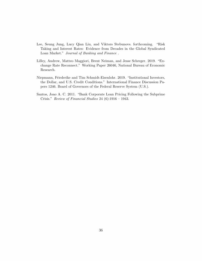
Specifically, global investors’ demand for leveraged loans responds to dollar

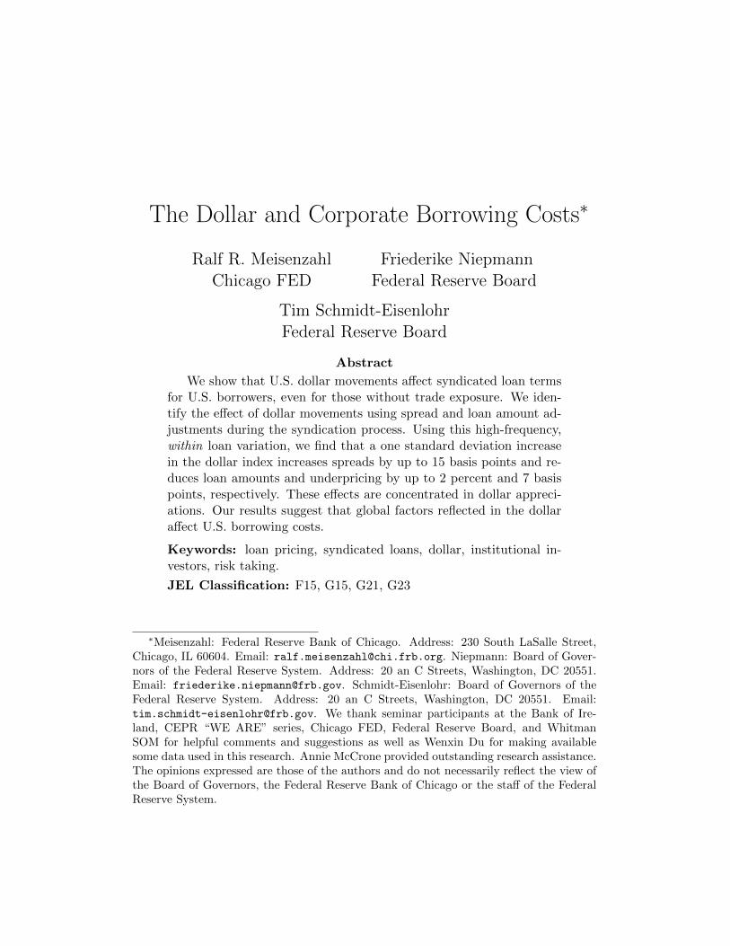
movements. Figure 1, showing that dollar appreciations are associated with

lower nonbank shares in newly formed syndicates, provides the first piece of

suggestive evidence for this claim.1 In this paper, we show that, as a conse-

quence of global demand linkages, global developments reflected in the dollar

directly affect the borrowing costs of U.S. corporations.

While a vast literature studies the effects of lender and borrower charac-

teristics or lender relationships on loan pricing, the effects of global develop-

ments on loan pricing are poorly understood.2 Furthermore, the direct effect

of dollar appreciations on U.S. borrowers adds a new aspect to the recent

international finance literature on “global financial cycles”. Since the global

financial crisis, the dollar has been shown to be a key variable affecting this

cycle.3 So far, this literature has documented how dollar cycles affect non-

U.S. countries. This paper shows that, through borrowing costs for risky

1The sharp drop in the nonbank share in late 2011 can be attributed to the Europeandebt crisis.

2See for example Ivashina (2009) and Santos (2011).3When the dollar appreciates, the capacity to bear risk in global capital markets tends

to fall, reflected in lower cross-border lending, larger CIP deviations, and a larger demandfor U.S. safe assets.

1

U.S. corporations, dollar cycles also affect the United States economy.4

Identifying the effect of macro-economic or global developments on cor-

porate borrowing costs is challenging and entails endogeneity issues in many

settings. To avoid these issues, most prominently those of borrower selection

and lower frequency confounding macroeconomic factors, we exploit the fact

that leveraged loan terms are adjusted during the syndication process, which

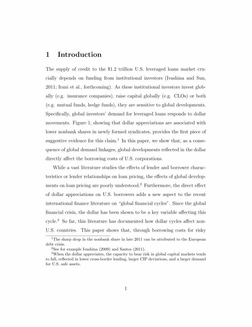
is illustrated in Figure 2.5 Specifically, we relate movements in the dollar dur-

ing the syndication process to differences between initial and final loan terms,

in a spirit similar to the identification in Bernstein (2015).6 Price adjustment

during the syndication process (flexes) offer a close-to-ideal setting to study

our question. First, initial loan terms are agreed upon by the borrower and

the lead arranger before the lead arranger assembles the syndicate—that

is, the borrower and key loan characteristics are fixed before demand for a

loan realizes, leaving no room for borrower selection. Second, initial loan

arranging agreements are designed to provide the lead arranger with strong

incentives to obtain the best possible loan terms for the borrower. There-

fore, adjustments of loan spreads, original issue discounts (primary market

discount), and loan amounts during the syndication process directly reflect

changes in the demand from outside investors for the given loan and are

independent of lead arranger characteristics.7 Finally, the syndication pro-

4An exception is Niepmann and Schmidt-Eisenlohr (2019), who show that U.S. banks’lending volumes and secondary market prices for corporate loans also move with the dollar.

5For more details on the syndication process, see Bruche, Malherbe, and Meisenzahl(forthcoming).

6Bernstein (2015) uses stock market movements during the IPO book building processas instrument for the completion of IPOs.

7Berg, Saunders, and Steffen (2016) document that discounts, sometimes labeled fees,play a significant role in loan pricing.

2

cess takes about two weeks, allowing us to use daily frequency data to tightly

identify the effect of dollar movements on prices and quantities, in contrast to

other studies focusing on quantities at the monthly or quarterly frequencies,

which may be affected by other macroeconomic factors.

We postulate that dollar appreciations lower the demand for risky assets

and derive testable hypotheses from book building theory applied to the loan

syndication process based on Bruche, Malherbe, and Meisenzahl (forthcom-

ing). First, changes in the effective spread during the syndication process

should be positively related to dollar movements. Second, changes in loan

amounts should be negatively related to dollar movements. Third, underpric-

ing, the difference between the primary market price and the first secondary

market price, should be negatively related to dollar movements.

Our main data source to test these hypotheses is the Leveraged Loan

Commentary and Data (LCD) that provides us with data on syndicated

leveraged loans from 2009-2019. In our main analysis, we keep only U.S.

borrowers. The data include the loan launch date, original (talk) loan terms

(amount, spread, original issue discount (OID), purpose and other loan char-

acteristics), adjustments to pricing terms (spread flex, OID flex) and to the

loan amount (amount flex) as well as the respective flex dates—the date on

which the loan started trading, and the first secondary market price.

The main explanatory variable is the change in the broad dollar index

during the syndication process for loans to U.S. corporations.8 We construct

this change as the difference in the broad dollar index between the start of the

book building process (launch date) and the date of pricing flexes (spread

8The broad dollar index is a trade-weighted average of the foreign exchange value ofthe U.S. dollar against the currencies of major U.S. trading partners.

3

and/or OID). The key outcome variable to test our first hypothesis is the

change in the effective spread (spread + OID/4) during the book building

process.9 We regress the change in the effective spread on the change in the

dollar index and, controlling for a rich set of loan characteristics such as the

initial (talk) loan spread, find that a one standard deviation change (about

one point) in the dollar index increases the final effective spread by 6 basis

points (bps). This increase is statistically significant and economically mean-

ingful, especially when considering that, on average, flexes to the effective

spread occur within 12 days from the loan launch date. When allowing for

asymmetric effects for dollar index increases and decreases, we find that a

one point increase in the dollar index is associated with a 15 bps increase

in the effective spread flex. These results represent the first evidence that

global shocks are transmitted through the dollar to borrowing costs of U.S.

corporations.

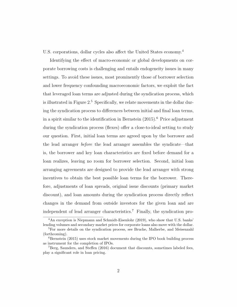
For context, we compare the estimated 15 bps increase in loan spreads at

origination to the response of secondary market prices of high-yield bonds.

Figure 3 shows that high-yield spreads on corporate bonds increased from

350 bps in mid-2014 to 800 bps in December 2015, while the dollar index

increased by 21 points, a 21 bps increase in spreads for a one point increase

in the dollar index, suggesting that primary and secondary market responses

are comparable in magnitude.10

Our primary market pricing result is robust to including loan and bor-

9We follow the market convention and ignore discounting. The typical maturity of aterm loan is 5 years. However, these loans are often refinanced earlier, so that the effectivematurity is closer to 4 years.

10The appendix shows the time series for the changes in both series. The correlationbetween the changes in the two series is 0.5.

4

rower characteristics as well as lead arranger fixed effects. To ensure that

our results are not driven by U.S. developments, we also control for changes

in the log VIX, the 2-year Treasury yield, the US term spread, the 3-month

U.S. Libor, the AAA-BBB corporate bond spread, the Aruoba-Diebold-Scotti

Business Conditions Index, and risk aversion and economic uncertainty from

Bekaert, Engstrom, and Xu (2019).11 We find that the coefficient on the

changes in the dollar index remains unchanged.

While we focus on U.S. borrowers only, one concern is that exposure to

dollar movements through imports or exports could be driving our results.

Such exposure would make borrowers’ credit risk sensitive to dollar movement

and, therefore, affect loan pricing. Our results are robust to restricting the

sample to loans to non-financial corporations and to non-tradable industries.

The estimate coefficients are in magnitude similar to the full sample. Hence,

international trade exposures do not account for our results.

One potential channel through which dollar movements could affect bor-

rowing costs is lead arranger’s balance sheet exposures to dollar movements.12

Consistent with dollar movements indicating investors’ demand for loans, we

find that interactions of U.S. lead arranger characteristics with dollar move-

ments have no effect on flexes. Non-U.S. lead arrangers do not drive our

results either. One reason for this finding is that arranging agreements pro-

vide strong incentives for the lead arranger to obtain the best loan terms

for the borrower. Indeed, we find that the changes to spreads during the

book building process are independent from lenders’ balance sheet exposures

11The Aruoba-Diebold-Scotti Business Conditions Index is designed to track real busi-ness conditions at high observation frequency.

12See Bruno and Shin (2015).

5

to dollar movements. We therefore conclude that the effect of the dollar on

U.S. borrowing costs is driven by changes in the demand from investors.

Next, we test our second hypothesis stating that loan amounts are nega-

tively related to dollar movements. Book building theory predicts that when

investors indicate low demand, the loan amount should be rationed (Ben-

veniste and Spindt, 1989). We find that loans that are syndicated during

a dollar appreciation the loan amount is decreased during the syndication

process and are less likely to exhibit a positive amount flex. A one standard

deviation (about 1 point) increase in the broad dollar index is associated

with 2 percent ($8 million) decrease in the loan amount. These results con-

stitute corroborating evidence that dollar appreciations indicate a reduction

in investors demand for leveraged loans and the transmission of global shock

to U.S. borrowers.

We then provide additional evidence that the dollar affects loan demand

by studying how dollar movements change loan syndicate participants’ rents,

measured as underpricing. By doing so, we test our third hypothesis. During

the book building process, arrangers incentivize participants to reveal their

demand for a loan by promising a rent for primary market participation.

This rent takes the form of underpricing—that is, the primary market price

is below the first secondary market price.13 We find that a one standard

13To reveal high demand, total rents—underpricing multiplied with amount allocatedto a participant—must be high. However, high demand usually leads to over-subscription,and therefore to lower allocated amounts and higher underpricing. Conversely, low de-mand increases allocated loan amounts and hence, arrangers can reduce underpricingwhile maintaining incentives to truthfully reveal demand during the book building process(Benveniste and Spindt, 1989; Bruche, Malherbe, and Meisenzahl, forthcoming). More-over, once the loan terms have been finalized but before the loan is actively traded in thesecondary market, movements in the dollar affect participants through their effects on thesecondary market price. Specifically, a dollar appreciation is associated with a decline in

6

deviation increase in the dollar index in the period between the launch date

and the first secondary market quote reduces underpricing by 2 percent. As

for spreads and loan amounts, the effect is larger for dollar appreciations.

The point estimate increases to 7 bps for a one point dollar appreciation.

To shed some light on the reasons why the dollar is associated with

the demand for risky assets, we include covered interest rate parity (CIP)

deviations—a proxy for financial intermediary arbitrage capital (Avdjiev

et al., 2019)—and the Treasury basis—a proxy for global demand for safe

assets (Jiang, Krishnamurthy, and Lustig, 2018) in the regressions. Con-

trolling for both, we find that the effect of dollar movements on spreads is

unchanged and that changes in CIP deviations have an independent, addi-

tional effect on spreads of U.S. corporate borrowers. The unchanged dollar

effect on spreads suggests a very tight link between the dollar and risky asset

demand, beyond the channels uncovered in the above papers. Independent

of the exact channels that link the dollar to investor demand for risky assets,

the dollar reflects the global price of dollar liquidity, which is affected by

global factors. Therefore, the dollar transmits global developments to U.S.

borrowers and the broader U.S. economy.

We contribute to several strands of the literature. First, we contribute to

the understanding of the dollar’s role for asset markets. Avdjiev et al. (2019)

document that a stronger dollar is associated with larger deviations from

covered interest parity and less cross-border bank lending. Jiang, Krishna-

murthy, and Lustig (2018) find that the dollar appreciates with the global

demand for U.S safe assets. Niepmann and Schmidt-Eisenlohr (2019) show

secondary market loan prices (Niepmann and Schmidt-Eisenlohr, 2019).

7

that dollar appreciations reduce secondary market loan prices and credit

supply from banks that follow an originate-to-distribute model. Lilley et al.

(2019) find that after the 2007-08 financial crisis the dollar co-moves with

global risk measures.14 Our high frequency results that dollar appreciations

lead to higher loan spreads are consistent with the view that the US dollar

is an indicator for the global demand for risky assets and that global shocks

affect U.S. domestic borrowing costs.

Second, we add to the literature on the syndication process and loan

prices. Ivashina and Sun (2011) show that loans that were syndicated during

times of lower inflows to funds take longer to syndicate and have higher

spreads. Bruche, Malherbe, and Meisenzahl (forthcoming) use the LCD data

to show that lead banks hold larger loan shares when investors demand is

low, using flex incidences as proxy for low demand. We add to their findings

by linking flex incidence to movements in the dollar index and therefore show

how global risk sentiment and global risk-taking capacity affect loan prices

for corporations.15

Third, we add to the growing literature that emphasizes the role of non-

banks and institutional investors in lending markets. Bord and Santos (2012).

Irani et al. (forthcoming), and Lee et al. (2019) document that nonbank par-

ticipants now account for 80 percent of leveraged loan holdings and that

nonbanks hold the most risky loans in this segment. Since collateralized

14Jiang, Krishnamurthy, and Lustig (2018) argue that changes in the convenience yieldassigned by foreign investors to U.S. Treasuries drive dollar movements.

15Since we only use within-loan variation, we implicitly control for other factors affectingloan pricing. For instance, Ivashina (2009) documents the impact of asymmetric informa-tion between the syndicated lead and participants on spreads. Santos (2011) links the leadbank’s financial health to syndicated loan spreads.

8

loan obligations (CLOs) and mutual funds cannot participate in the primary

market they often pre-arrange buying loan shares from participating banks,

who originate to distribute these shares. Consistent with this originate-

to-distribute model, Lee, Liu, and Stebunovs (forthcoming) document the

increasing share of nonbanks directly after the syndication process is com-

pleted.16 Our findings show that the US dollar is an indicator for the demand

of such investors for risky assets.

The remainder of the paper is organized as follows. Section 2 describes

our data. In section 3, we develop our testable hypothesis. The empirical

results are presented in section 4. In section 5, we assess the effects of CIP

deviations and movements in the Treasury basis. Section 6 concludes.

2 Data

Our main data source is S&P Capital IQ’s Leveraged Commentary and Data

(LCD). LCD contains detailed data on leveraged loans, their characteristics,

and their syndication process. The data set includes syndicated loans with

either a non-investment-grade rating, or with a first or second lien and a

spread of at least 125 basis points over LIBOR.17

In our analysis, we focus on loans originated between 2009 and 2019 for

two reasons. First, a crucial measure of loan riskiness, the talk yield—the

loan yield used by the lead bank to start the book-running—is only consis-

tently available from 2009 on. Second, by excluding prior years, we ensure

16However, there is little evidence that nonbank participation increases adverse selection(Benmelech, Dlugosz, and Ivashina, 2012).

17Figure A1 shows the distribution of loan ratings for the sample.

9

that our results are not driven by the 2007-08 financial crisis. In addition,

we only keep U.S. borrowers to exclude the possibility that borrowers’ credit

risk is directly affected by dollar movements.18

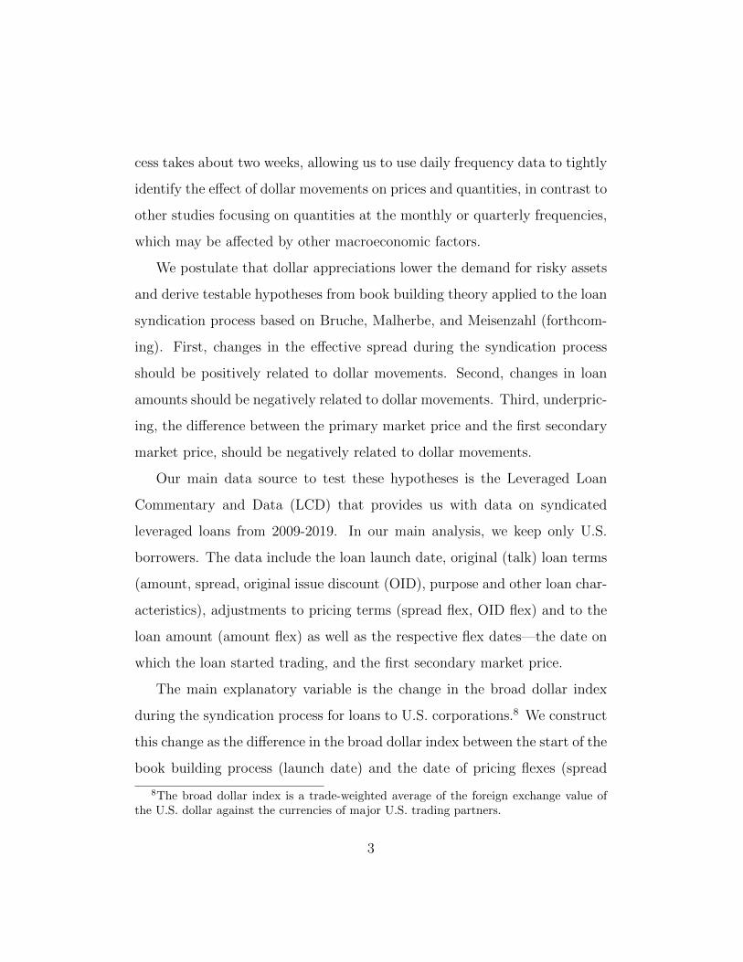
Figure 4 shows the monthly number of loans and monthly total loan

amounts in the institutional leveraged term loan market during the sample

period. While leveraged loan originations were subdued at the beginning of

the sample, we observe on average 58 loans per month.19 Over the sample

period, the loan amounts add up to $2.5 trillion.

Our main variables of interest are the adjustments (flexes) to the spread,

the original issue discount, the loan amount, and the first secondary mar-

ket loan price. The data contain the corresponding launch, flex, and break

dates of these variables. Figure 5 shows the incidences of positive (negative)

flexes to the effective spread and the loan amount. The figure shows that

adjustments to loan terms are common. Moreover, positive and negative flex

incidences exhibit a clear, negative correlation for both effective spread flex

and amount flex.

Using the launch date, the flex date, and the date of the first secondary

market price, we construct changes in the broad dollar index for the time from

launch date to flex date and from flex date to first secondary market price

date. The broad dollar index is a trade-weighted dollar exchange rate index

calculated and published as part of the weekly H.10-Foreign Exchange Rate

18To identify U.S. borrowers in the LCD data, we merge LCD data with Dealscan dataand information from the Loan Syndications and Trading Association (LSTA).

19In late 2015/early 2016 the primary market for syndicated loans effectively shut downin the wake of a failed syndication. The arrangers were not able to assemble a syndicateto finance the take-over of Veritas. The low demand for this loan, which market partici-pants attributed in hindsight to CLO industry concentration limits (preventing CLOs frominvesting in this deal), as well as uncertainty about CLO oil exposures spooked investors.

10

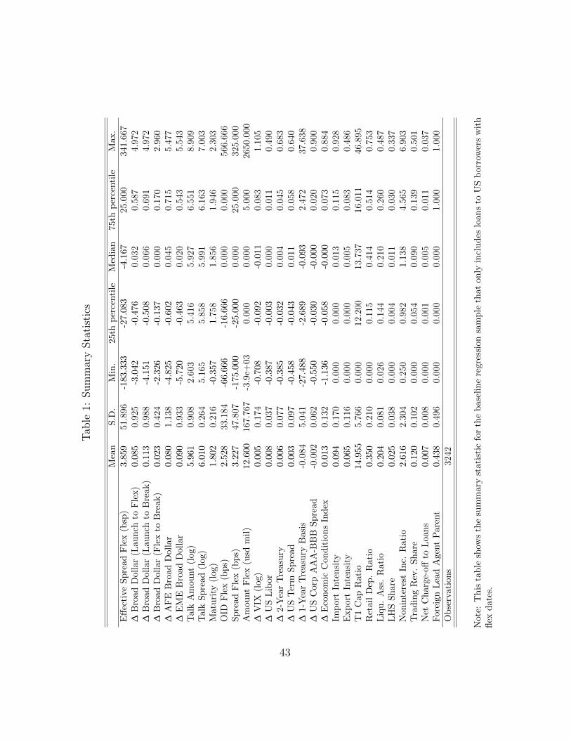
release by the Board of Governors of the Federal Reserve System.20 Table 1

presents the summary statistics for the LCD sample, the broad dollar index,

and additional control variables, including U.S. financial market variables

and bank balance sheet variables.21

3 Hypothesis Development

In the development of our testable hypothesis, we focus on the implications of

book building theory because Bruche, Malherbe, and Meisenzahl (forthcom-

ing) document that syndication is a book building process.22 We first briefly

summarize the syndication process and then derive testable hypotheses.

The Syndication Process

The syndication process, illustrated in Figure 2, starts with borrowers

soliciting bids including pricing and risk-sharing provisions from arrangers.

The borrower awards the mandate to the preferred arranger. The arranger

then proposes a facility agreement that includes all loan terms such as the

interest rate, the original issue discount, covenants, and repayment options

and uses this agreement to market the loan to investors.

The marketing or book running takes place in at least one round. In

20The trade partners included in the broad dollar index calculations are the Euro Area,Canada, Japan, Mexico, China, United Kingdom, Taiwan, Korea, Singapore, Hong Kong,Malaysia, Brazil, Switzerland, Thailand, Philippines, Australia, Indonesia, India, Israel,Saudi Arabia, Russia, Sweden, Argentina, Venezuela, Chile, and Colombia.

21All variables are described in Appendix A, table A1.22For detailed description of the syndication process, see Bruche, Malherbe, and Meisen-

zahl (forthcoming). For more details and test of book building theory especially in thecontext of IPOs, see Benveniste and Spindt (1989), Hanley (1993), and Cornelli and Gol-dreich (2003).

11

each round, the arranger proposes a facility agreement including all loan

terms such as the pricing to investors. If, given proposed loan terms, there is

sufficient demand, the loan is originated at those terms. If the demand from

the loan is higher or lower, then there is another round. Based on demand

that realized with the last set of loan terms, the arranger “flexes,” that is,

adjusts the terms accordingly. For instance, if demand was low, then the

arranger may increase the interest rate or decrease the loan amount in the

next round. The ability to flex, the range of flexes, and the consequences

of flexes for the arranger’s fee are part of the risk-sharing in the contract

between borrower and arranger. The process continues until the loan is

originated. After the borrower received the funds, the loan starts trading in

the secondary loan market.

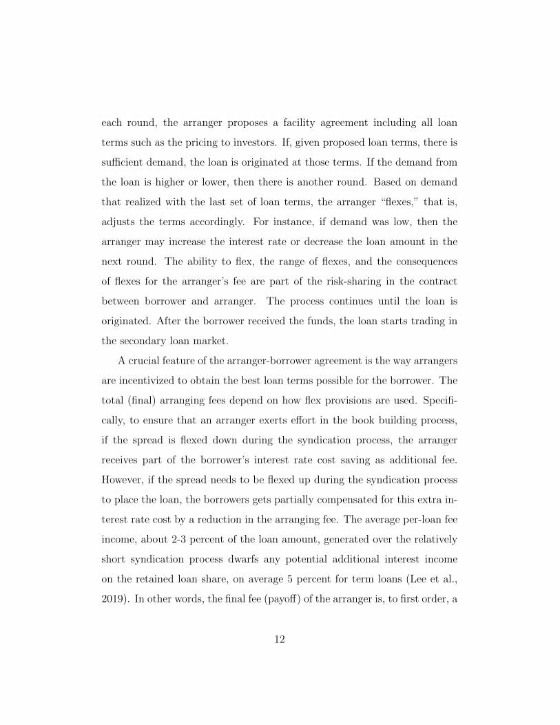
A crucial feature of the arranger-borrower agreement is the way arrangers

are incentivized to obtain the best loan terms possible for the borrower. The

total (final) arranging fees depend on how flex provisions are used. Specifi-

cally, to ensure that an arranger exerts effort in the book building process,

if the spread is flexed down during the syndication process, the arranger

receives part of the borrower’s interest rate cost saving as additional fee.

However, if the spread needs to be flexed up during the syndication process

to place the loan, the borrowers gets partially compensated for this extra in-

terest rate cost by a reduction in the arranging fee. The average per-loan fee

income, about 2-3 percent of the loan amount, generated over the relatively

short syndication process dwarfs any potential additional interest income

on the retained loan share, on average 5 percent for term loans (Lee et al.,

2019). In other words, the final fee (payoff) of the arranger is, to first order, a

12

function of loan term adjustments and final loan terms that the borrower re-

ceives.23 As such, the changes in loan terms during the book building process

should be independent from the lead arranger’s balance sheet.

Testable Hypothesis

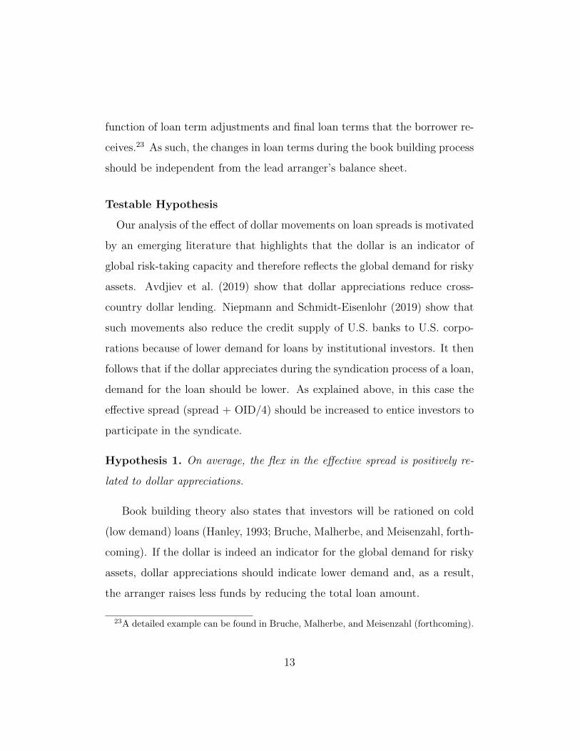
Our analysis of the effect of dollar movements on loan spreads is motivated

by an emerging literature that highlights that the dollar is an indicator of

global risk-taking capacity and therefore reflects the global demand for risky

assets. Avdjiev et al. (2019) show that dollar appreciations reduce cross-

country dollar lending. Niepmann and Schmidt-Eisenlohr (2019) show that

such movements also reduce the credit supply of U.S. banks to U.S. corpo-

rations because of lower demand for loans by institutional investors. It then

follows that if the dollar appreciates during the syndication process of a loan,

demand for the loan should be lower. As explained above, in this case the

effective spread (spread + OID/4) should be increased to entice investors to

participate in the syndicate.

Hypothesis 1. On average, the flex in the effective spread is positively re-

lated to dollar appreciations.

Book building theory also states that investors will be rationed on cold

(low demand) loans (Hanley, 1993; Bruche, Malherbe, and Meisenzahl, forth-

coming). If the dollar is indeed an indicator for the global demand for risky

assets, dollar appreciations should indicate lower demand and, as a result,

the arranger raises less funds by reducing the total loan amount.

23A detailed example can be found in Bruche, Malherbe, and Meisenzahl (forthcoming).

13

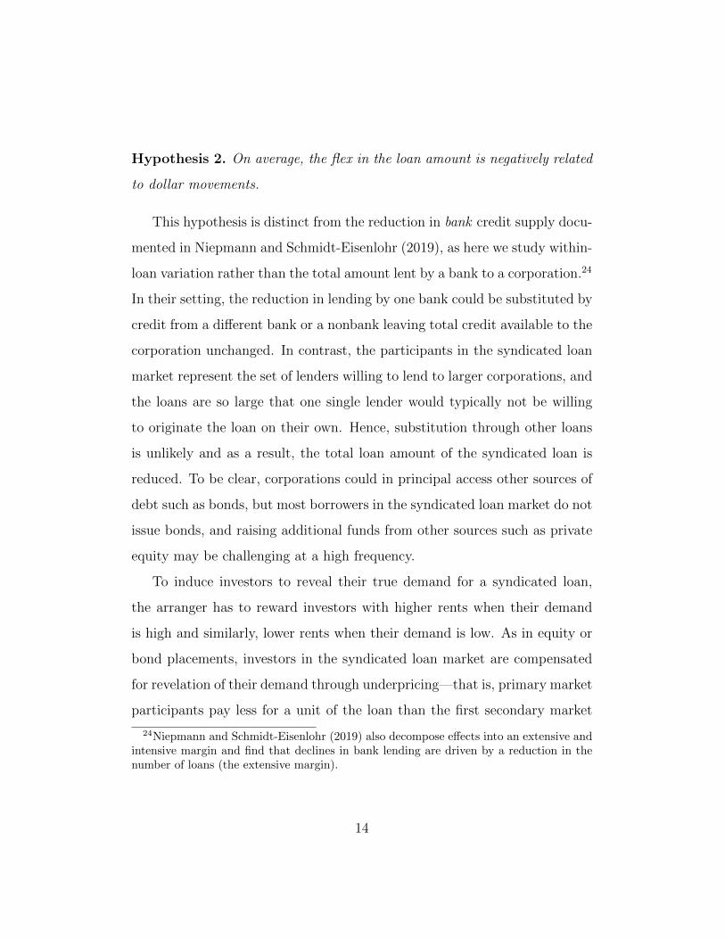
Hypothesis 2. On average, the flex in the loan amount is negatively related

to dollar movements.

This hypothesis is distinct from the reduction in bank credit supply docu-

mented in Niepmann and Schmidt-Eisenlohr (2019), as here we study within-

loan variation rather than the total amount lent by a bank to a corporation.24

In their setting, the reduction in lending by one bank could be substituted by

credit from a different bank or a nonbank leaving total credit available to the

corporation unchanged. In contrast, the participants in the syndicated loan

market represent the set of lenders willing to lend to larger corporations, and

the loans are so large that one single lender would typically not be willing

to originate the loan on their own. Hence, substitution through other loans

is unlikely and as a result, the total loan amount of the syndicated loan is

reduced. To be clear, corporations could in principal access other sources of

debt such as bonds, but most borrowers in the syndicated loan market do not

issue bonds, and raising additional funds from other sources such as private

equity may be challenging at a high frequency.

To induce investors to reveal their true demand for a syndicated loan,

the arranger has to reward investors with higher rents when their demand

is high and similarly, lower rents when their demand is low. As in equity or

bond placements, investors in the syndicated loan market are compensated

for revelation of their demand through underpricing—that is, primary market

participants pay less for a unit of the loan than the first secondary market

24Niepmann and Schmidt-Eisenlohr (2019) also decompose effects into an extensive andintensive margin and find that declines in bank lending are driven by a reduction in thenumber of loans (the extensive margin).

14

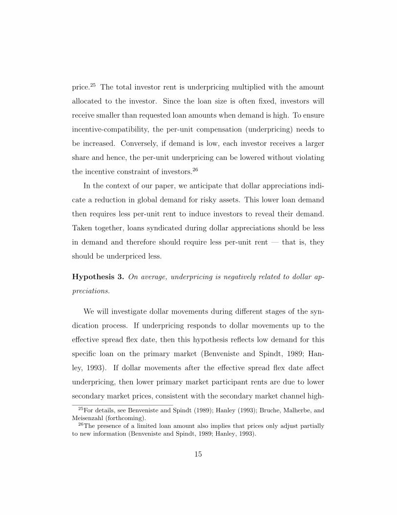
price.25 The total investor rent is underpricing multiplied with the amount

allocated to the investor. Since the loan size is often fixed, investors will

receive smaller than requested loan amounts when demand is high. To ensure

incentive-compatibility, the per-unit compensation (underpricing) needs to

be increased. Conversely, if demand is low, each investor receives a larger

share and hence, the per-unit underpricing can be lowered without violating

the incentive constraint of investors.26

In the context of our paper, we anticipate that dollar appreciations indi-

cate a reduction in global demand for risky assets. This lower loan demand

then requires less per-unit rent to induce investors to reveal their demand.

Taken together, loans syndicated during dollar appreciations should be less

in demand and therefore should require less per-unit rent — that is, they

should be underpriced less.

Hypothesis 3. On average, underpricing is negatively related to dollar ap-

preciations.

We will investigate dollar movements during different stages of the syn-

dication process. If underpricing responds to dollar movements up to the

effective spread flex date, then this hypothesis reflects low demand for this

specific loan on the primary market (Benveniste and Spindt, 1989; Han-

ley, 1993). If dollar movements after the effective spread flex date affect

underpricing, then lower primary market participant rents are due to lower

secondary market prices, consistent with the secondary market channel high-

25For details, see Benveniste and Spindt (1989); Hanley (1993); Bruche, Malherbe, andMeisenzahl (forthcoming).

26The presence of a limited loan amount also implies that prices only adjust partiallyto new information (Benveniste and Spindt, 1989; Hanley, 1993).

15

lighted by Niepmann and Schmidt-Eisenlohr (2019).

4 Corporate Borrowing Costs and the Dollar

In this section, we conduct our empirical analysis. We first study the effect

of changes in the dollar during the book-running process on effective loan

spreads and whether these effects vary by loan characteristics. We then turn

to loan amounts. Last, we analyze whether underpricing—the rent earned by

primary market syndicate participants—is affected by changes in the dollar.

4.1 The Dollar and Syndicated Loan Terms

We start our empirical analysis by assessing the effect of changes in the dollar

on the change in the effective spread. The effective spread is easy to calculate

since syndicated loans have a floating rate, typically comprised of LIBOR as

base rate and the effective spread (spread + OID/4).27 To isolate this effect,

we focus on dollar movements during the syndication process—that is, we

focus on the changes in the effective spread during the syndication process,

while holding borrower and loan characteristics constant. By focusing on this

within-loan variation, we avoid potential borrower selection and can separate

the effect of dollar movements as they are orthogonal to other potential loan-

specific factors that can explain loan spreads.28

27Later, we directly control for an extensive set of macroeconomic, financial, and mone-tary controls, including the 2-year Treasury yield and the term spread in case that changesin the base rate affect the effective spread.

28For instance, Ivashina (2009) studies the effect of asymmetric information on loanspreads. Our identification strategy is similar to Bernstein (2015), who uses stock marketmovements after the initial IPO filings as an instrument for IPO completion.

16

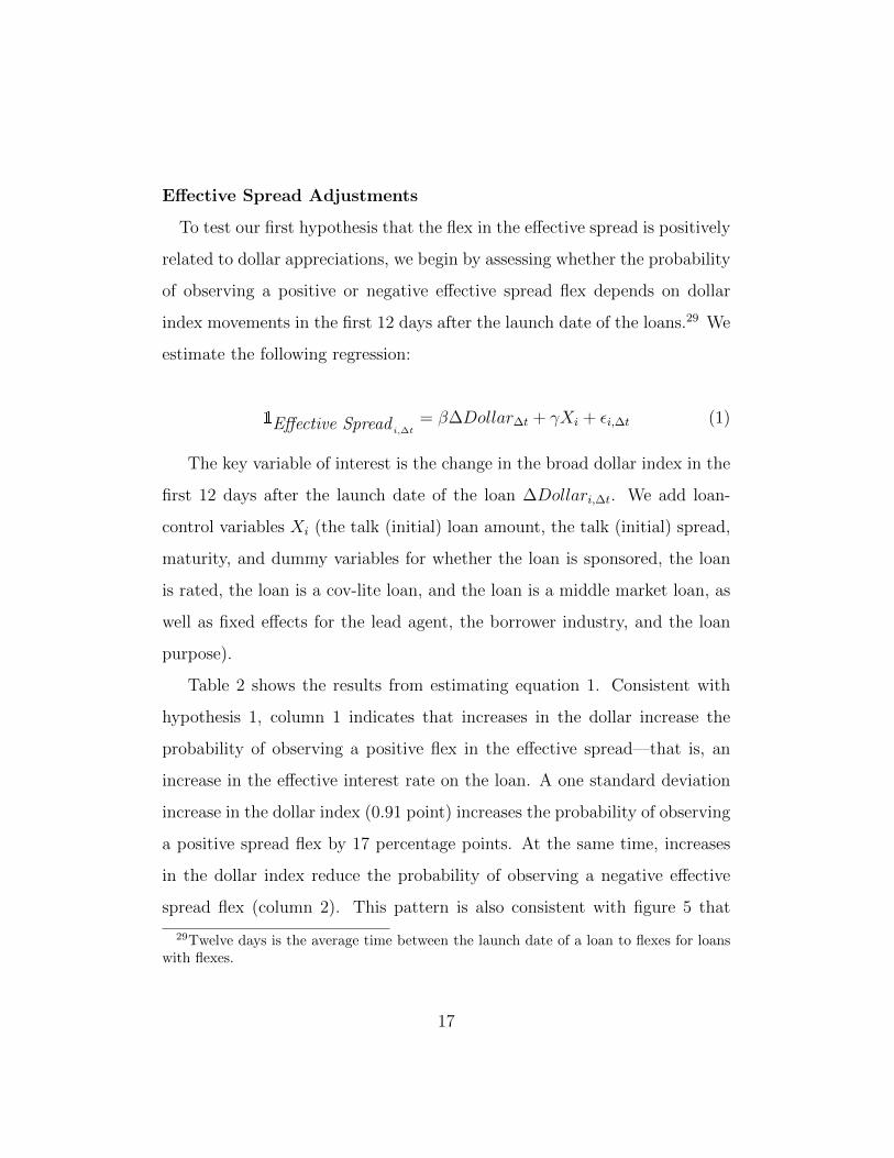
Effective Spread Adjustments

To test our first hypothesis that the flex in the effective spread is positively

related to dollar appreciations, we begin by assessing whether the probability

of observing a positive or negative effective spread flex depends on dollar

index movements in the first 12 days after the launch date of the loans.29 We

estimate the following regression:

1Effective Spread i,∆t= β∆Dollar∆t + γXi + εi,∆t (1)

The key variable of interest is the change in the broad dollar index in the

first 12 days after the launch date of the loan ∆Dollari,∆t. We add loan-

control variables Xi (the talk (initial) loan amount, the talk (initial) spread,

maturity, and dummy variables for whether the loan is sponsored, the loan

is rated, the loan is a cov-lite loan, and the loan is a middle market loan, as

well as fixed effects for the lead agent, the borrower industry, and the loan

purpose).

Table 2 shows the results from estimating equation 1. Consistent with

hypothesis 1, column 1 indicates that increases in the dollar increase the

probability of observing a positive flex in the effective spread—that is, an

increase in the effective interest rate on the loan. A one standard deviation

increase in the dollar index (0.91 point) increases the probability of observing

a positive spread flex by 17 percentage points. At the same time, increases

in the dollar index reduce the probability of observing a negative effective

spread flex (column 2). This pattern is also consistent with figure 5 that

29Twelve days is the average time between the launch date of a loan to flexes for loanswith flexes.

17

shows a negative correlation between positive and negative flexes. Restricting

the sample to loans with a flex date, we find that these effects are more

pronounced (columns 3 and 4). These results show that borrowers are more

likely to face higher-than-expected effective interest rates on syndicated loans

if the dollar appreciates during the first two weeks of the syndication process.

This finding is consistent with the view that an appreciation of the dollar

indicates lower global demand for risky assets.

Having established that positive flexes in the effective spread are more

likely with dollar index increases, we now inspect the relationship between

the size of the effective spread flex and dollar movements. Figure 6 plots

the data binned by dollar index movements and the corresponding effective

spread flex. There is a clear correlation between effective spread flexes and

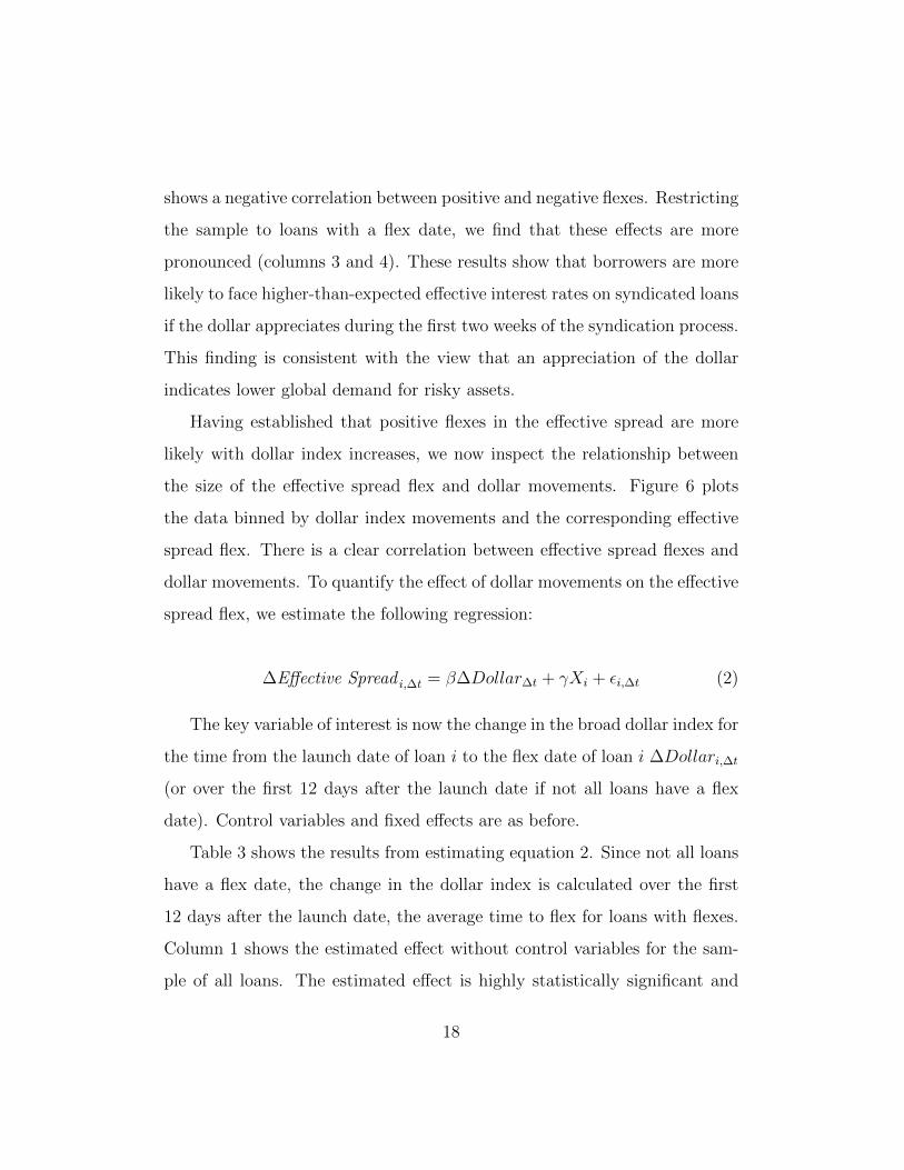
dollar movements. To quantify the effect of dollar movements on the effective

spread flex, we estimate the following regression:

∆Effective Spread i,∆t = β∆Dollar∆t + γXi + εi,∆t (2)

The key variable of interest is now the change in the broad dollar index for

the time from the launch date of loan i to the flex date of loan i ∆Dollari,∆t

(or over the first 12 days after the launch date if not all loans have a flex

date). Control variables and fixed effects are as before.

Table 3 shows the results from estimating equation 2. Since not all loans

have a flex date, the change in the dollar index is calculated over the first

12 days after the launch date, the average time to flex for loans with flexes.

Column 1 shows the estimated effect without control variables for the sam-

ple of all loans. The estimated effect is highly statistically significant and

18

suggests that a one standard deviation (0.91 points) increase in the dollar

index increases the effective loan spread by 2.4 basis points. In column 2,

we add loan-level controls, including the talk (initial) spread to account for

the ex-ante riskiness of the loan, and find that the coefficient on the dollar

index change and its statistical significance remains unchanged. This result

is robust to the inclusion of borrower industry, loan purpose and lead bank

fixed effects (column 3).

We repeat these regressions for the sample of loans for which we observe

the flex date, and the change in the dollar index is calculated from the launch

date to the flex date. Table 3, column 4 shows the estimated effect without

control variables. Compared to column 1, the coefficient is more than twice

as large. A one standard deviation increase in the dollar index increases the

effective loan spread by 6 basis points. Adding controls (column 5) and fixed

effects (column 6) does not change the estimated effect. The stability of the

coefficient across specifications suggests that changes in the effective spread

are in fact driven by changes in the dollar index and not by unobserved loan

characteristics.30

A potential concern with our specification and interpretation is that

changes in the dollar index could reflect other macroeconomic developments

such as increases in economic uncertainty or other relevant news. To ensure

that our results are not driven by such developments, we augment equa-

tion 2 by adding the changes in a large set of U.S. variables. Specifically,

we use changes in the log VIX, the US Corporate AAA-BBB spread, the

30In unreported results, we find no evidence for heterogeneous effects of dollar move-ments by credit rating, talk spread, or loan size. One potential reason is that leverage loansare deemed to be a non-investment grade asset class and changes in the risk sentimentreduce the demand for the whole assets class and not just for the riskiest parts.

19

2-year Treasury yield, the U.S. term spread, the 3-month U.S. Libor, and

the Aruoba-Diebold-Scotti Business Conditions Index as proxies for U.S. fi-

nancial and macroeconomic conditions.31 Since syndicated term loans are

floating rate loans, changes in the level of short-term interest rates should

not affect the spread.

Table 4 shows the results of adding changes in macroeconomic variables to

equation 2. In columns 1 and 2, we subsequently add controls for changes in

U.S. macroeconomic conditions and loan controls. When adding all macroe-

conomic controls, the coefficient shown in column 2 (5.471) is only slightly

smaller compared to the baseline results without macroeconomic controls

(6.496, shown in Table 3, column 5). Adding industry, purpose, lead bank

fixed effect does not not materially affect the size of the estimated coefficient

(column 3) either. Controlling for syndication quarter fixed effects, which

partly absorb the changes in the dollar index, reduces this coefficient in size,

but the effect remains sizable and statistically significant (column 4). Taken

together, the results indicate that changes in the dollar index do not sim-

ply reflect other observable changes in the U.S. financial and macroeconomic

environment.32

31We include the VIX as measure of uncertainty in the economy. The US CorporateAAA-BBB spread is a proxy for the risk premium with compressed spreads indicatinga low risk premium. We include the 3-month U.S. Libor and the 2-year Treasury yieldas measures of short-term and medium-term interest rates, and the U.S. term spread asmeasure of future economic conditions. The Aruoba-Diebold-Scotti Business ConditionsIndex captures U.S. business conditions at high frequency.

32In section 5, we demonstrate the robustness of our results to controlling for changesin CIP deviations and the Treasury basis. In addition, table B3 in the appendix in-cludes changes in risk aversion and economic uncertainty from Bekaert, Engstrom, andXu (2019) as control variables, with no effects on the magnitude nor the significance of thedollar coefficient. In unreported results, we find that the inclusion of changes in Japanesemacroeconomic conditions also does not affect our main result.

20

Controlling for International Exposures

Changes in the broad dollar may directly affect a borrower’s revenues and

costs if the borrower imports, exports, or has cross-border financial activities.

This may in turn affect the ability of a borrower to repay a loan and hence

the credit spread charged by banks. We address this concern by dropping

loans for financial corporations and by showing that our results hold in the

sample of firms in non -tradable sectors.

Table 5 shows results for all loans with a flex.33 Columns 1 and 2 show

the baseline results when excluding the financial sector (all SIC codes start-

ing with 6), as banks and other financial institutions often transact across

borders. Our main results are unaffected by the exclusion of the financial

sector.

To ensure that our results are not driven by the trade exposures of bor-

rowers, we split the sample into non-traded and traded industries. Columns

3 and 4 show results for the baseline specification for industries that do not

export or import (as before, we are also excluding the financial sector). The

baseline results remain, which implies that even firms with no exports or

imports face higher financing costs when the dollar appreciates. Finally,

columns 5 and 6 repeat the baseline specification for all firms in industries

with some exports or imports. While the point estimates are somewhat larger

than those in columns 3 and 4, they are not significantly different.

We conclude that the effect we uncover is neither driven by export or

import exposures of borrowers nor is it driven by financial sector borrowers

33Note that industry fixed effects in table 5 are based on borrowers’ SIC codes. SICcodes are not available for all borrowers in the dataset. Therefore industry fixed effects inother tables are implemented using a less granular industry classification that is availablein the LCD data.

21

with financial links across borders.

The Role of Lead Agent Characteristics

While studying price adjustments during the syndication process alle-

viates concerns about borrower selection, it is possible that time-varying

lead arranger characteristics affect price adjustments during the syndication

process—that is, flexes could be driven by dollar exposures of lead arrangers’

balance sheets rather than by the demand for the loans from investors. For

instance, if lead banks fund loans through wholesale dollar markets, sudden

dollar movements affect the lead arranger’s funding cost. However, if the

dollar reflects investor demand, then lead arranger characteristics should not

affect the flexes.

The arranger agreement is designed to provide the lead arranger with

strong incentives to obtain the best possible loan terms for the borrower.

As described in section 3, the arranger agreement makes the lead arranger’s

payoff a function of flexes during the syndication process. Moreover, lead ar-

rangers only retain a small loan share, reducing the benefits of higher interest

rates for the arranger. Taken together, this incentive structure implies time-

varying lead arranger characteristics should not matter for effective spread

flexes.

To test whether lead arrangers’ characteristics affect flexes, we draw on

balance sheet information contained in the Y-9C reports of 21 U.S. lead

arrangers.34 These 21 lead agents arrange around 84 percent of the loans in

the sample. We compute lagged four-quarter rolling averages of the following

34Foreign banks that do not operate BHCs or IHCs in the U.S. and nonbanks such asNomura or Jefferies Securities do not have to file regulatory reports.

22

lead-agent characteristics: Tier 1 capital ratio, retail deposit share, liquid

asset ratio, share of loans held for sale (LHS share), non-interest income

ratio, share of trading revenues in non-interest plus interest income, and

ratio of net charge-offs to total loans.35

We conduct our analysis in parallel to column 6 of table 3. We use the

subsample of loans to U.S borrowers that have a flex date and include loan

controls as well as industry, purpose and lead fixed effects. In addition, we

interact the lead bank characteristics with the change in the dollar index and

include the linear and the interaction terms in the regressions.

Table 6 shows the results. Consistent with our hypothesis that lead ar-

ranger characteristics do not affect flexes, none of the interactions terms are

statistically significant. Moreover, for all specifications, the point estimate

on the change in the dollar index is very similar to the baseline point estimate

shown in column 6 of table 3. We therefore conclude that lead arrangers’

exposure to dollar movements do not play a role for price adjustments during

the syndication process.36

To ensure that our results are not driven by non-U.S. lead arrangers

that arguably are exposed to dollar movements by having to raise dollar

funding for syndicated loans, we now test for differences in the effect of

the dollar on the effective spread flex between U.S. lead arrangers and lead

arrangers with foreign parents. Accordingly, we define a dummy variable

Foreign Lead Arranger Parent that takes the value of 1 if the lead arranger

35Details on the construction of the lead-arranger variables can be found in table A1.36We ran different variants of the effective spread flex regressions, including various

fixed effects as controls and using a sample that includes all loans. The interaction termsbetween the dollar and lead arranger characteristics were not statistically significant inthese alternative specifications.

23

is owned by a foreign parent and interact this dummy with the change in the

dollar index. We include these variables in the baseline regression.

Table 7 shows the results. As indicated by columns 1 and 2, the point

estimate on Foreign Lead Arranger Parent is economically small and sta-

tistically insignificant for the full sample. This finding holds in the subsample

of loans with flexes (columns 3 and 4).

In sum, neither lead arranger balance sheet exposures to dollar move-

ments nor differences in responses to dollar movements between domestic

and foreign lead arrangers account for the observed changes in the flexes in

response to dollar movement. This finding is consistent with dollar move-

ments reflecting the demand for loans by investors.

Loan Amount Adjustments

Last, we complement the evidence on loan pricing with evidence on loan

amounts. Specifically, when investors’ demand for a loan is low, the lead

agent should not only increase the effective spread but also decrease the loan

amount (Hanley, 1993; Bruche, Malherbe, and Meisenzahl, forthcoming). To

test this hypothesis (hypothesis 2) we estimate the following regression:

∆Loan Amount i,∆t = β∆Dollar∆t + γXi + εi,∆t, (3)

where ∆Loan Amount i,∆t is either the change in the loan amount or an in-

dicator variable that the loan amount was flexed down (up).

Table 8 shows the results from estimating equation 3. Column 1 shows

that movements in the dollar index negatively affect loan amounts, but the

effect is statistically insignificant. This effect increases and becomes statically

24

significant in the subsample of loans with an amount flex, shown in column

2, to $8 million (2 percent).

In column 3 (4), we estimate the propensity of observing a positive (nega-

tive) amount flex. A 1 point increase in the dollar index reduces the propen-

sity of observing a positive amount flex, an increase in the loan amount during

the syndication process, by 12 percent. However, we do not find evidence

that dollar movements affect the propensity of negative spread flexes.

In sum, reductions in loan amount during the syndication process driven

by dollar appreciations are consistent with dollar appreciations indicating

lower investor demand for risky assets and show that credit supply to large

U.S. corporations is critically affected by institutional investors.

4.2 Dollar Exposure of Syndicate Participants

We now turn to the effect of changes in the dollar on primary market partic-

ipant rents. To induce investors in the primary market to reveal their true

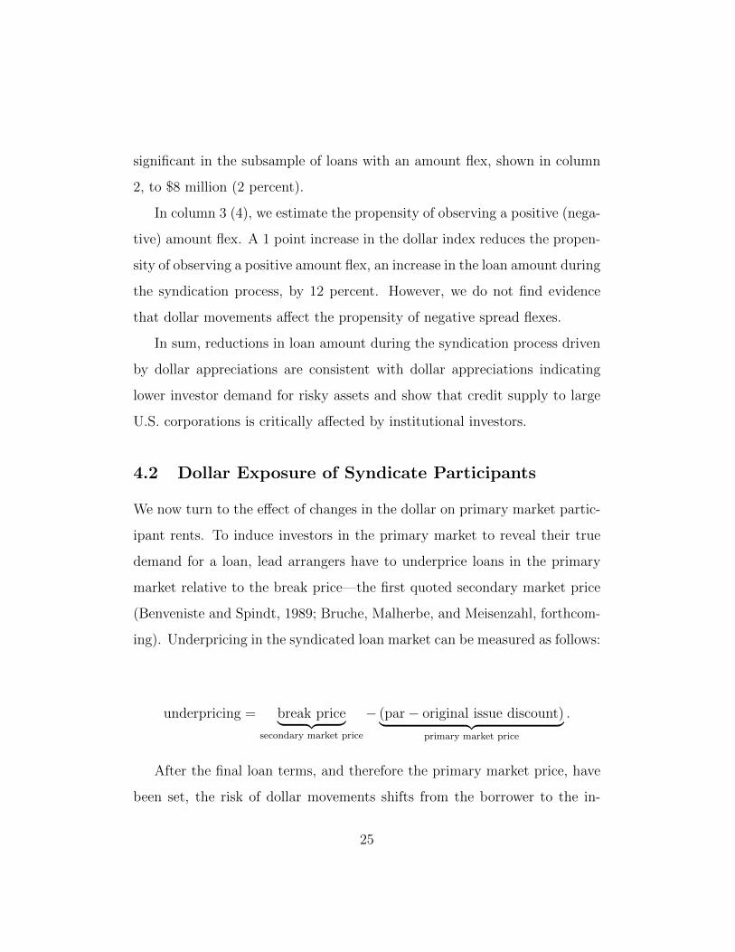
demand for a loan, lead arrangers have to underprice loans in the primary

market relative to the break price—the first quoted secondary market price

(Benveniste and Spindt, 1989; Bruche, Malherbe, and Meisenzahl, forthcom-

ing). Underpricing in the syndicated loan market can be measured as follows:

underpricing = break price︸︷︷︸secondary market price

− (par − original issue discount)︸︷︷︸primary market price

.

After the final loan terms, and therefore the primary market price, have

been set, the risk of dollar movements shifts from the borrower to the in-

25

vestors before the loan starts trading in the secondary market. Niepmann

and Schmidt-Eisenlohr (2019) show that dollar appreciations reduce sec-

ondary market prices for syndicated loans in general.37 Therefore, dollar

appreciations should affect underpricing negatively.

To test our third hypothesis that underpricing is negatively related to

dollar appreciations, we estimate the following regression:

Underpricing i = β∆Dollar∆t + γXi + εi,∆t, (4)

where ∆Dollar∆t is now the change in the dollar index between the flex date

(the date of final loan terms) and the break price date (the date of the first

secondary market price quote).

Table 9 shows the results of estimating equation 4. Increases in the dollar

during the syndication process are not fully reflected in the effective spread

and reduce primary market participant rents (column 2).38 The effect is

slightly larger when considering the changes over the whole syndication pro-

cess (column 1). The risk of changes in underpricing after the effective spread

is flexed but before the loan starts trading is fully borne by syndicate par-

ticipants. In fact, increases in the dollar after the flex date also reduce

underpricing (column 3) even though the average time from the flex date to

the break price date is only one day. This reduction is driven by declines

in loan prices on the secondary market in response to dollar appreciations.

This finding is consistent with the secondary market channel documented by

37Irani and Meisenzahl (2017) show that liquidity pressures on banks leads to more loansales and reduces prices for loans previously held by banks.

38This results is consistent with partial adjustment during the book building process(Benveniste and Spindt, 1989; Bruche, Malherbe, and Meisenzahl, forthcoming).

26

Niepmann and Schmidt-Eisenlohr (2019).

Bruche, Malherbe, and Meisenzahl (forthcoming) report that, on average,

underpricing in the syndicated loan market is about 45 bps over a comparable

sample period.39 Our results therefore suggest that a one standard deviation

increase in the dollar index reduces primary market participants’ rent by 2

bps.

In sum, the results presented in this section show that movements in the

dollar affect primary market participants’ rents. Loan interest rates only

partially price the changes in the dollar index from the launch date to the

flex date. Lower secondary market prices in response to increases in the

dollar index can reduce underpricing after the final loan pricing is set.

4.3 Asymmetric Effect of Dollar Movements

In this section, we test whether the effects of increases and decreases of the

dollar index are symmetric. Figure 6 suggests a potential asymmetry as the

correlation between dollar movements and spread flex appears to be stronger

for dollar index increases than for decreases.

To test whether the effect of dollar index increases and decreases are

symmetric, we estimate the following regression:

∆Outcome i,∆t = β11∆Dollar∆t>0∆Dollar∆t (5)

+ β21∆Dollar∆t<0∆Dollar∆t + γXi + εi,∆t

39This is somewhat higher than the underpricing for bonds (Cai, Helwege, and Warga,2007).

27

The regression equation also includes a dummy variable for very small

changes in the dollar, meaning −0.025 ≤ ∆Dollar ≤ 0.025. Table 10 shows

the results of estimating equation 5 with changes in the dollar index split

into appreciations, dollar depreciations, and very small changes in the dollar.

Column 1 shows that our results for the effective spread flex are driven by

dollar appreciations rather than depreciations. While the effect of increases

in the dollar index (β1) is economically large and statistically significant,

the effect of decreases in the dollar index (β2) is economically small and

statistically insignificant. This pattern holds for both components of the

effective spread flex, the OID flex (column 2) and the spread flex (column

3). The asymmetric effects of dollar appreciations and depreciations are also

present in the amount flex (column 4) and in underpricing (column 5).

The economic significance of increases in the dollar index is substantially

larger than the average effects estimated before. Specifically, a standard de-

viation increase in the dollar index increases the spread by 15.2 bps compared

to 6 bps shown in table 3, column 5, and the effect on underpricing more

than doubles to 6.1 bps compared to 2 bps based in table 9, column 1. The

effect on the loan amount—a $8 million reduction in the loan amounts—is

the same as in the linear specification shown in table 8, column 2.

The asymmetric results indicate asymmetries in the response of institu-

tional investors’ loan demand to changes in the dollar. One potential expla-

nation for this could be asymmetric hedging as suggested by Koutmos and

Martin (2003). However, since we do not have data on hedging or derivative

contracts held by nonbank financial institutions, we cannot test this hypothe-

sis. Future research should investigate the possible causes of the asymmetries

28

we document.

5 CIP Deviations, Safe Asset Demand, and

the Dollar

So far, we have shown that the dollar affects the borrowing costs of U.S. cor-

porations, consistent with the dollar reflecting investor demand for leveraged

loans. Why is it that the dollar reflects investors’ appetite for risky assets?

The literature offers several explanations.40

First, Avdjiev et al. (2019) show that the dollar exchange rate is corre-

lated with CIP deviations, which arguably proxy the capacity of financial

intermediaries to engage in arbitrage activities. When the arbitrage capital

of financial intermediaries globally becomes scarcer, reflected in bigger CIP

deviations, the dollar tends to appreciate. Second, Jiang, Krishnamurthy,

and Lustig (2018) argue that the dollar appreciates with the global demand

for safe assets, finding that convenience yields on U.S. Treasuries correlate

positively with the dollar exchange rate. Third, Bruno and Shin (2015) show

how global currency-mismatches imply a worsening of financial intermedi-

aries’ balance-sheets when the dollar appreciates, tightening value-at-risk

constraints and thereby reducing risk-taking.41

In the following we test if the first two channels above explain the rela-

tionship between the dollar and U.S. borrowing costs. Results are presented

40See Du (Forthcoming) for a review of the literature.41In theoretical work, Gabaix and Maggiori (2015) show how financial intermediaries

price currency risk and, thereby, affect the level of exchange rates. Akinci and Queralto(2018), model a two-way relationship between balance sheet strength of borrowers and thedollar.

29

in Table 11. For ease of comparison, column 1 presents again the baseline re-

sults from table 3, column 6, showing the effect of changes in the dollar index

on flexes. Column 2 adds a measure of CIP deviations, the average five-year

dollar Libor cross-currency basis against G10 currencies from Avdjiev et al.

(2019). This Libor basis is almost always negative over the sample period.

Increases in the Libor basis reflect, on average, smaller CIP deviations and,

hence, greater financial intermediary capacity. As expected, an increase in

the Libor basis (a less negative Libor basis) is associated with smaller flexes,

as indicated by the negative, significant coefficient. However, the inclusion of

CIP deviations reduces the coefficient on dollar changes only somewhat and

the dollar effect continues to be highly statistically significant. This suggests

that the dollar effect on corporate borrowing costs goes beyond any effect

that works through the financial intermediary arbitrage capital channel.42

Column 3 of table 11 employs changes in the 1-year Treasury basis from

Du, Im, and Schreger (2018).43 A larger Treasury basis implies that investors

are willing to pay a higher premium to hold U.S. Treasuries compared to

other safe securities. Accordingly, a higher Treasury basis should be associ-

ated with less risk-taking and, hence, larger flexes. However, in contrast to

this conjecture, conditional on dollar movements a higher Treasury basis is

associated with lower flexes, as column 3 shows.44 This finding suggests that

42In the appendix, table B2, columns 7 and 8 show that CIP deviations have a significanteffect on flexes without the inclusion of dollar. Moreover, we can include CIP deviationsalong with the dollar in all specifications, and both coefficients will always be significant(Results available upon request.) These additional results suggest that CIP deviationsaffect U.S. corporate borrowing costs independently from the dollar.

43We obtain similar results when using 3-month, 2-year, 3-year, 5-year, 7-year, or 10-yeartreasury basis instead of the 1-year Treasury basis.

44In table B2 in the appendix, we show that when including only the Treasury basis,the point estimate is still negative but statistically insignificant, suggesting that safe asset

30

the dollar effect on corporate borrowing costs is not driven by a differential

demand for U.S. safe assets.

Column 4 controls for both CIP deviations and the Treasury basis at the

same time. In columns 5, U.S. financial and macroeconomic variables are

added. Column 6 incorporates additionally year-quarter fixed effects. The

estimated dollar coefficients are hardly changed compared with the equivalent

regressions without CIP deviations and Treasury basis.

Besides reflecting financial intermediary capacity, larger CIP deviations

imply that the cost of obtaining dollars in swap markets is larger for foreign

investors without direct access to dollar funding. Because the U.S. leveraged

loan market attracts foreign investors that may finance their investments

through FX swaps, larger CIP deviations may make leveraged loans less

attractive for this group. Whether CIP deviations affect borrowing costs

through this direct link or through a more indirect channel cannot be con-

clusively answered based on the regressions presented here. In any case, the

fact that CIP deviations affect U.S. corporate borrowing costs is additional

evidence that U.S. borrowing costs depend on global factors.45

If neither the safe asset demand channel reflected in the Treasury nor

global financial intermediary capacity reflected in CIP deviations fully ex-

plain the effect of the dollar on U.S. corporate borrowing costs, what other

channel can connect the dollar to investor demand for risky assets? It is pos-

demand as measured by the treasury basis is of lesser importance for corporate borrowingcosts.

45Another conjecture is that financial regulation that has reduced financial intermedi-aries’ arbitrage capital may have indirectly increased the borrowing costs for U.S. corpo-rations. In this context, see Eguren-Martin, Ossandon Busch, and Reinhardt (2019) whofind that banks reduce their cross-border lending in response to larger CIP deviations.

31

sible that changes in the dollar exchange rate alter the risk profile of global

investors’ portfolios, making them riskier in the spirit of Bruno and Shin

(2015). In this case, exogenous shocks to the dollar exchange rate would

directly affect investors’ risky asset demand and U.S. corporate borrowing

costs.

Since we control for U.S. macroecomomic and financial variables, and

because of our high-frequency identification and robustness of our results,

U.S. factors are unlikely to drive our results. Instead, our results point to

a close connection between the dollar exchange rate and investor demand

for risky assets. The broad dollar index captures the global price of dollar

liquidity and is driven, to a significant degree, by non-U.S. developments.

Therefore, regardless of the exact mechanism that links the dollar to the

investor demand for risky assets, we conclude that, through the dollar, global

shocks transmit to U.S. corporate borrowing costs.

6 Conclusion

We show that movements in the dollar index materially affect the corporate

borrowing cost and credit supply to U.S. corporate borrowers. Using high

frequency data and within-loan identification, we find that the effects are con-

centrated in increases in the dollar index. These results are consistent with

the interpretation that dollar movements reflect changes in global risk senti-

ment and the global demand for risky assets. As we showed, the relationship

between the dollar and borrowing costs persists even when controlling for

CIP deviations that capture financial intermediary constraints and the con-

32

venience yield that measures the premium associated with holding U.S. safe

assets. While it is beyond the scope of our paper to pin down the channels

that connect the dollar to investors’ demand for risky assets, our results show

that through the dollar, which is driven by non-U.S. factors, global factors

affect U.S. borrowing costs and through that the broader U.S. economy.

33

References

Akinci, Ozge and Albert Queralto. 2018. “Exchange Rate Dynamics and MonetarySpillovers with Imperfect Financial Markets.” Staff Repor 849, Federal ReserveBank of New York t.

Avdjiev, Stefan, Wenxin Du, Cathrine Koch, and Hyun Song Shin. 2019. “TheDollar, Bank Leverage, and Deviations from Covered Interest Parity.” AmericanEconomic Review: Insights 1 (2):193–208.

Bekaert, Geert, Eric C. Engstrom, and Nancy R. Xu. 2019. “The Time Variationin Risk Appetite and Uncertainty.” NBER Working Papers 25673, NationalBureau of Economic Research, Inc.

Benmelech, Efraim, Jennifer Dlugosz, and Victoria Ivashina. 2012. “Securitizationwithout adverse selection: The case of CLOs.” Journal of Financial Economics106 (1):91–113.

Benveniste, Lawrence M. and Paul A. Spindt. 1989. “How investment bankersdetermine the offer price and allocation of new issues.” Journal of FinancialEconomics 24 (2):343–361.

Berg, Tobias, Anthony Saunders, and Sascha Steffen. 2016. “The Total Cost ofCorporate Borrowing in the Loan Market: Don’t Ignore the Fees.” Journal ofFinance 71 (3):1357–1392.

Bernstein, Shai. 2015. “Does Going Public Affect Innovation?” Journal of Finance70 (4):1365–1403.

Bord, Vitaly M. and Joao A. C. Santos. 2012. “The Rise of the Originate-to-Distribute Model and the Role of Banks in Financial Intermediation.” FederalReserve Bank of New York Economic Policy Review 18 (2):21 – 34.

Bruche, Max, Frederic Malherbe, and Ralf R. Meisenzahl. forthcoming. “PipelineRisk in Leveraged Loan Syndication.” Review of Financial Studies .

Bruno, Valentina and Hyun Song Shin. 2015. “Cross-border banking and globalliquidity.” Review of Economic Studies 82 (2):535–564.

Cai, Nianyun (Kelly), Jean Helwege, and Arthur Warga. 2007. “Underpricing inthe Corporate Bond Market.” Review of Financial Studies 20 (6):2021–2046.

Cornelli, Francesca and David Goldreich. 2003. “Bookbuilding: How InformativeIs the Order Book?” Journal of Finance 58 (4):1415–1443.

34

Du, Wenxin. Forthcoming. “Financial Intermediation Channel in the Global DollarCycle.” 2019 Jackson Hole Economic Policy Symposium Proceedings .

Du, Wenxin, Joanne Im, and Jesse Schreger. 2018. “The US Treasury Premium.”Journal of International Economics 112:167–181.

Eguren-Martin, Fernando, Matias Ossandon Busch, and Dennis Reinhardt. 2019.“Global banks and synthetic funding: the benefits of foreign relatives.” Bankof England working papers 762, Bank of England.

Gabaix, Xavier and Matteo Maggiori. 2015. “International liquidity and exchangerate dynamics.” The Quarterly Journal of Economics 130 (3):1369–1420.

Hanley, Kathleen Weiss. 1993. “The underpricing of initial public offerings and thepartial adjustment phenomenon.” Journal of Financial Economics 34 (2):231–250.

Irani, Rustom, Rajkamal Iyer, Ralf R. Meisenzahl, and Jose-Luis Peydro. forth-coming. “The Rise of Shadow Banking: Evidence from Capital Regulation.”Review of Financial Studies .

Irani, Rustom and Ralf R. Meisenzahl. 2017. “Loan Sales and Bank LiquidityManagement: Evidence from a U.S. Credit Register.” Review of FinancialStudies 30 (10):3455–3501.

Ivashina, Victoria. 2009. “Asymmetric information effects on loan spreads.” Jour-nal of Financial Economics 92 (2):300 – 319.

Ivashina, Victoria and Zheng Sun. 2011. “Institutional demand pressure and thecost of corporate loans.” Journal of Financial Economics 99 (3):500 – 522.

Jiang, Zhengyang, Arvind Krishnamurthy, and Hanno Lustig. 2018. “Foreign SafeAsset Demand for US Treasurys and the Dollar.” AEA Papers and Proceedings108:537–41.

Koutmos, Gregory and Anna D Martin. 2003. “Asymmetric exchange rate ex-posure: theory and evidence.” Journal of international Money and Finance22 (3):365–383.

Lee, Seung Jung, Dan Li, Ralf R. Meisenzahl, and Martin Sicilian. 2019. “TheU.S. Syndicated Term Loan Market: Who holds what and when?” FEDS Notes,November 25, 2019. Board of Governors of the Federal Reserve System (U.S.).

35

Lee, Seung Jung, Lucy Qian Liu, and Viktors Stebunovs. forthcoming. “RiskTaking and Interest Rates: Evidence from Decades in the Global SyndicatedLoan Market.” Journal of Banking and Finance .

Lilley, Andrew, Matteo Maggiori, Brent Neiman, and Jesse Schreger. 2019. “Ex-change Rate Reconnect.” Working Paper 26046, National Bureau of EconomicResearch.

Niepmann, Friederike and Tim Schmidt-Eisenlohr. 2019. “Institutional Investors,the Dollar, and U.S. Credit Conditions.” International Finance Discussion Pa-pers 1246. Board of Governors of the Federal Reserve System (U.S.).

Santos, Joao A. C. 2011. “Bank Corporate Loan Pricing Following the SubprimeCrisis.” Review of Financial Studies 24 (6):1916 – 1943.

36

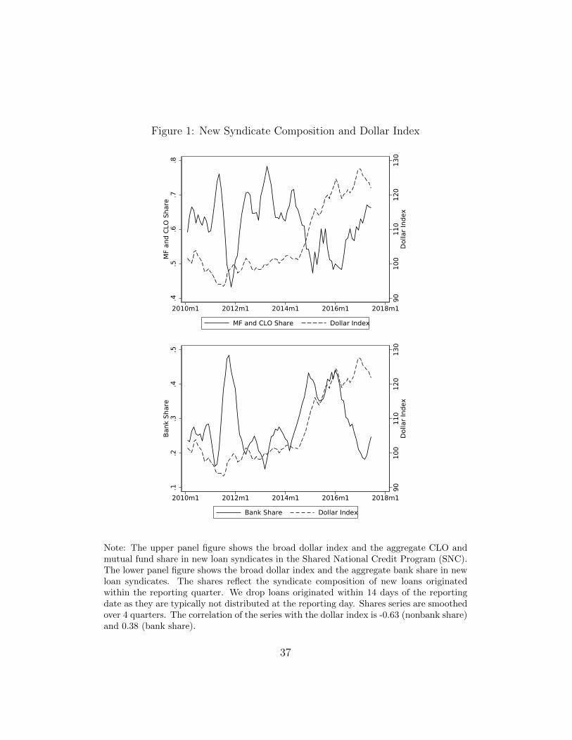
Figure 1: New Syndicate Composition and Dollar Index

9010

011

012

013

0D

olla

r Ind

ex

.4.5

.6.7

.8M

F an

d CL

O S

hare

2010m1 2012m1 2014m1 2016m1 2018m1

MF and CLO Share Dollar Index

9010

011

012

013

0D

olla

r Ind

ex

.1.2

.3.4

.5Ba

nk S

hare

2010m1 2012m1 2014m1 2016m1 2018m1

Bank Share Dollar Index

Note: The upper panel figure shows the broad dollar index and the aggregate CLO andmutual fund share in new loan syndicates in the Shared National Credit Program (SNC).The lower panel figure shows the broad dollar index and the aggregate bank share in newloan syndicates. The shares reflect the syndicate composition of new loans originatedwithin the reporting quarter. We drop loans originated within 14 days of the reportingdate as they are typically not distributed at the reporting day. Shares series are smoothedover 4 quarters. The correlation of the series with the dollar index is -0.63 (nonbank share)and 0.38 (bank share).

37

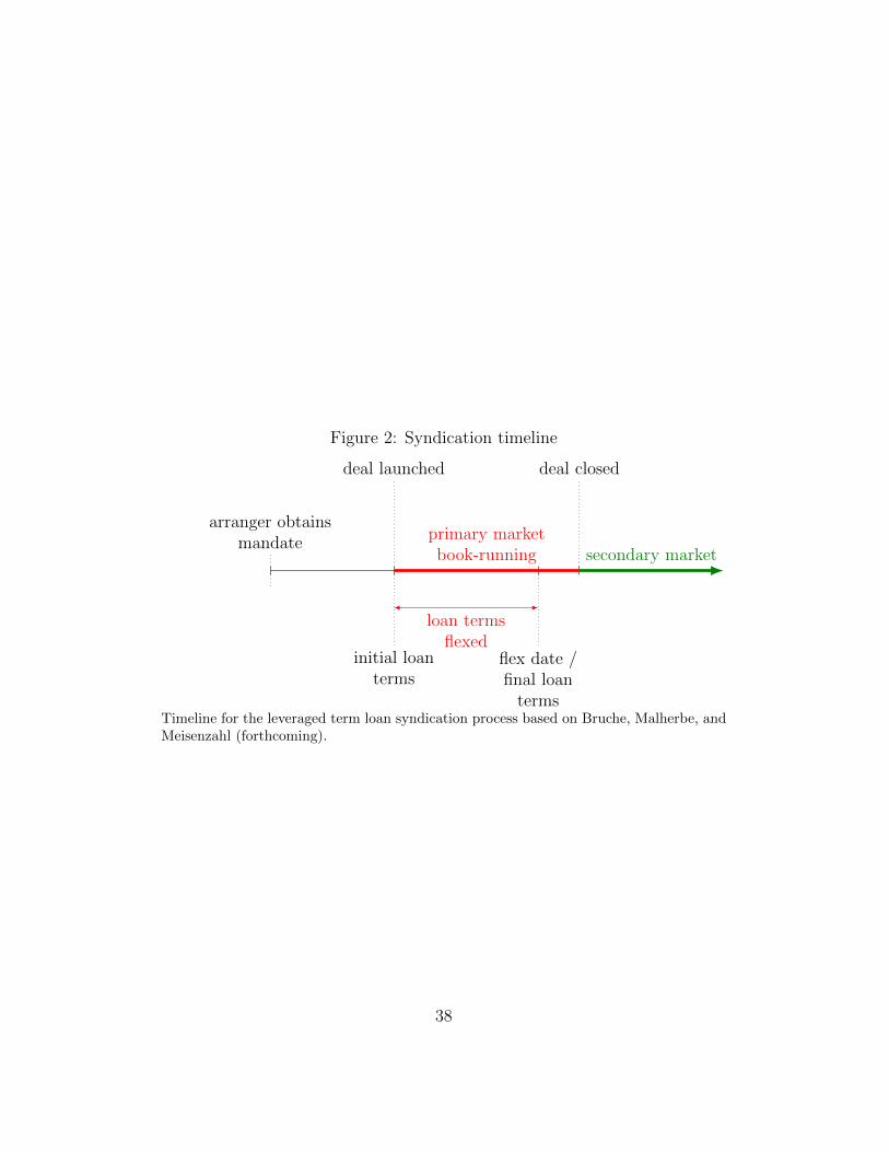
Figure 2: Syndication timeline

arranger obtainsmandate

initial loanterms

deal launched deal closed

flex date /final loan

terms

primary marketbook-running

loan termsflexed

secondary market

Timeline for the leveraged term loan syndication process based on Bruche, Malherbe, andMeisenzahl (forthcoming).

38

Figure 3: High Yield Spread and the Dollar Index

Note: The figure shows the broad dollar index and the US high yield spread from 2009 to2019. The high yield spread is the Master II Option-Adjusted Spread from FRED.

39

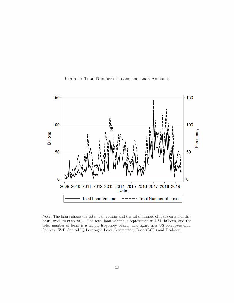
Figure 4: Total Number of Loans and Loan Amounts

Note: The figure shows the total loan volume and the total number of loans on a monthlybasis, from 2009 to 2019. The total loan volume is represented in USD billions, and thetotal number of loans is a simple frequency count. The figure uses US-borrowers only.Sources: S&P Capital IQ Leveraged Loan Commentary Data (LCD) and Dealscan.

40

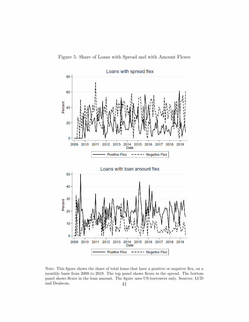
Figure 5: Share of Loans with Spread and with Amount Flexes

Note: This figure shows the share of total loans that have a positive or negative flex, on amonthly basis from 2009 to 2019. The top panel shows flexes in the spread. The bottompanel shows flexes in the loan amount. The figure uses US-borrowers only. Sources: LCDand Dealscan. 41

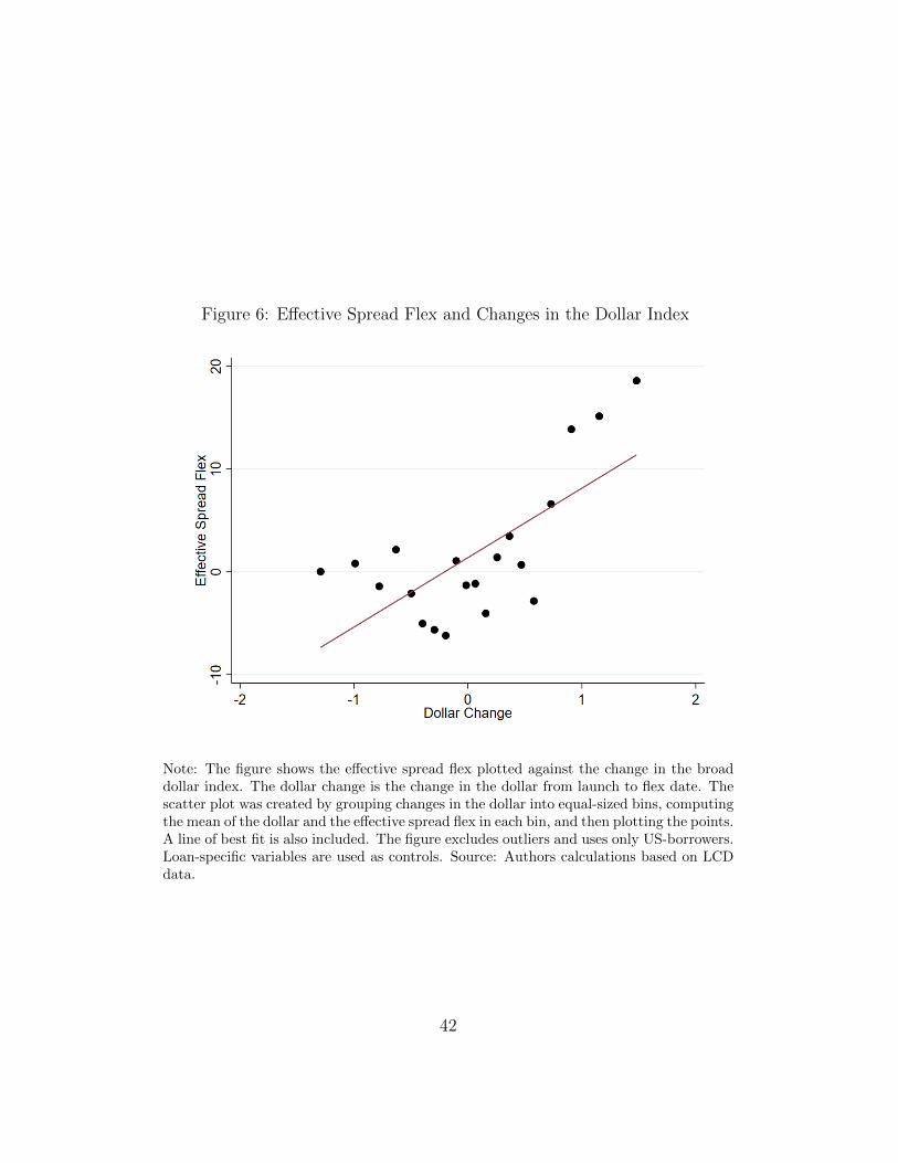
Figure 6: Effective Spread Flex and Changes in the Dollar Index

Note: The figure shows the effective spread flex plotted against the change in the broaddollar index. The dollar change is the change in the dollar from launch to flex date. Thescatter plot was created by grouping changes in the dollar into equal-sized bins, computingthe mean of the dollar and the effective spread flex in each bin, and then plotting the points.A line of best fit is also included. The figure excludes outliers and uses only US-borrowers.Loan-specific variables are used as controls. Source: Authors calculations based on LCDdata.

42

Tab

le1:

Sum

mar

ySta

tist

ics

Mea

nS

.D.

Min

.25th

per

centi

leM

edia

n75th

per

centi

leM

ax.

Eff

ecti

veS

pre

adF

lex

(bsp

)3.

859

51.8

96

-183.3

33

-27.0

83

-4.1

67

25.0

00

341.6

67

∆B

road

Dol

lar

(Lau

nch

toF

lex)

0.08

50.9

25

-3.0

42

-0.4

76

0.0

32

0.5

87

4.9

72

∆B

road

Dol

lar

(Lau

nch

toB

reak

)0.

113

0.9

88

-4.1

51

-0.5

08

0.0

66

0.6

91

4.9

72

∆B

road

Dol

lar

(Fle

xto

Bre

ak)

0.02

30.4

24

-2.3

26

-0.1

37

0.0

00

0.1

70

2.9

60

∆A

FE

Bro

adD

olla

r0.

080

1.1

38

-4.8

25

-0.6

02

0.0

45

0.7

15

5.4

77

∆E

ME

Bro

adD

olla

r0.

090

0.9

33

-5.7

20

-0.4

63

0.0

20

0.5

43

5.5

43

Tal

kA

mou

nt

(log

)5.

961

0.9

08

2.6

03

5.4

16

5.9

27

6.5

51

8.9

09

Tal

kS

pre

ad(l

og)

6.01

00.2

64

5.1

65

5.8

58

5.9

91

6.1

63

7.0

03

Mat

uri

ty(l

og)

1.80

20.2

16

-0.3

57

1.7

58

1.8

56

1.9

46

2.3

03

OID

Fle

x(b

ps)

2.52

833.1

84

-66.6

66

-16.6

66

0.0

00

0.0

00

566.6

66

Sp

read

Fle

x(b

ps)

3.22

747.8

07

-175.0

00

-25.0

00

0.0

00

25.0

00

325.0

00

Am

ount

Fle

x(u

sdm

il)

12.6

00167.7

67

-3.9

e+03

0.0

00

0.0

00

5.0

00

2650.0

00

∆V

IX(l

og)

0.00

50.1

74

-0.7

08

-0.0

92

-0.0

11

0.0

83

1.1

05

∆U

SL

ibor

0.00

80.0

37

-0.3

87

-0.0

03

0.0

00

0.0

11

0.4

90

∆2-

Yea

rT

reas

ury

0.00

60.0

77

-0.3

85

-0.0

32

0.0

04

0.0

45

0.6

83

∆U

ST

erm

Sp

read

0.00

30.0

97

-0.4

58

-0.0

43

0.0

11

0.0

58

0.6

40

∆1-

Yea

rT

reas

ury

Bas

is-0

.084

5.0

41

-27.4

88

-2.6

89

-0.0

93

2.4

72

37.6

38

∆U

SC

orp

AA

A-B

BB

Sp

read

-0.0

020.0

62

-0.5

50

-0.0

30

-0.0

00

0.0

20

0.9

00

∆E

con

omic

Con

dit

ion

sIn

dex

0.01

30.1

32

-1.1

36

-0.0

58

-0.0

00

0.0

73

0.8

84

Imp

ort

Inte

nsi

ty0.

094

0.1

70

0.0

00

0.0

00

0.0

13

0.1

15

0.9

28

Exp

ort

Inte

nsi

ty0.

065

0.1

16

0.0

00

0.0

00

0.0

05

0.0

83

0.4

86

T1

Cap

Rat

io14

.955

5.7

66

0.0

00

12.2

00

13.7

37

16.0

11

46.8

95

Ret

ail

Dep

.R

atio

0.35

00.2

10

0.0

00

0.1

15

0.4

14

0.5

14

0.7

53

Liq

u.

Ass

.R

atio

0.20

40.0

81

0.0

26

0.1

44

0.2

10

0.2

60

0.4

87

LH

SS

har

e0.

025

0.0

38

0.0

00

0.0

04

0.0

11

0.0

30

0.3

37

Non

inte

rest

Inc.

Rat

io2.

616

2.3

04

0.2

50

0.9

82

1.1

38

4.5

65

6.9

03

Tra

din

gR

ev.

Sh

are

0.12

00.1

02

0.0

00

0.0

54

0.0

90

0.1

39

0.5

01

Net

Ch

arge

-off

toL

oan

s0.

007

0.0

08

0.0

00

0.0

01

0.0

05

0.0

11

0.0

37

For

eign

Lea

dA

gent

Par

ent

0.43

80.4

96

0.0

00

0.0

00

0.0

00

1.0

00

1.0

00

Ob

serv

atio

ns

3242

Not

e:T

his

tab

lesh

ows

the

sum

mar

yst

atis

tic

for

the

base

lin

ere

gre

ssio

nsa

mp

leth

at

on

lyin

clu

des

loan

sto

US

borr

ower

sw

ith

flex

dat

es.

43

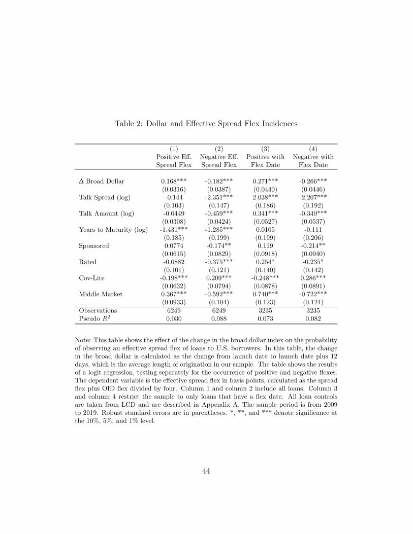
Table 2: Dollar and Effective Spread Flex Incidences

(1) (2) (3) (4)Positive Eff. Negative Eff. Positive with Negative withSpread Flex Spread Flex Flex Date Flex Date

∆ Broad Dollar 0.168*** -0.182*** 0.271*** -0.266***(0.0316) (0.0387) (0.0440) (0.0446)

Talk Spread (log) -0.144 -2.351*** 2.038*** -2.207***(0.103) (0.147) (0.186) (0.192)

Talk Amount (log) -0.0449 -0.459*** 0.341*** -0.349***(0.0308) (0.0424) (0.0527) (0.0537)

Years to Maturity (log) -1.431*** -1.285*** 0.0105 -0.111(0.185) (0.199) (0.199) (0.206)

Sponsored 0.0774 -0.174** 0.119 -0.214**(0.0615) (0.0829) (0.0918) (0.0940)

Rated -0.0882 -0.375*** 0.254* -0.235*(0.101) (0.121) (0.140) (0.142)

Cov-Lite -0.198*** 0.209*** -0.248*** 0.286***(0.0632) (0.0794) (0.0878) (0.0891)

Middle Market 0.367*** -0.592*** 0.740*** -0.722***(0.0933) (0.104) (0.123) (0.124)

Observations 6249 6249 3235 3235Pseudo R2 0.030 0.088 0.073 0.082

Note: This table shows the effect of the change in the broad dollar index on the probabilityof observing an effective spread flex of loans to U.S. borrowers. In this table, the changein the broad dollar is calculated as the change from launch date to launch date plus 12days, which is the average length of origination in our sample. The table shows the resultsof a logit regression, testing separately for the occurrence of positive and negative flexes.The dependent variable is the effective spread flex in basis points, calculated as the spreadflex plus OID flex divided by four. Column 1 and column 2 include all loans. Column 3and column 4 restrict the sample to only loans that have a flex date. All loan controlsare taken from LCD and are described in Appendix A. The sample period is from 2009to 2019. Robust standard errors are in parentheses. *, **, and *** denote significance atthe 10%, 5%, and 1% level.

44

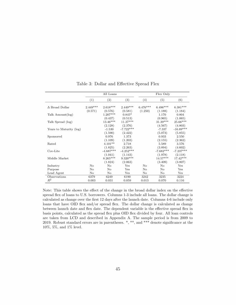
Table 3: Dollar and Effective Spread Flex

All Loans Flex Only

(1) (2) (3) (4) (5) (6)

∆ Broad Dollar 2.449*** 2.618*** 2.449*** 6.476*** 6.496*** 6.381***(0.571) (0.576) (0.581) (1.250) (1.188) (1.184)

Talk Amount(log) 1.207*** 0.845* 1.170 0.804(0.437) (0.513) (0.965) (1.065)

Talk Spread (log) 13.46*** 11.37*** 31.39*** 25.66***(2.128) (2.376) (4.567) (4.803)

Years to Maturity (log) -1.530 -7.722*** -7.337 -16.89***(1.590) (2.422) (5.073) (5.855)

Sponsored 0.976 1.373 0.933 2.550(1.109) (1.203) (2.155) (2.362)

Rated 4.101** 2.718 5.589 3.576(1.825) (2.263) (3.894) (4.602)

Cov-Lite -4.687*** -4.252*** -7.682*** -7.237***(1.041) (1.143) (1.978) (2.118)

Middle Market 8.265*** 9.320*** 14.57*** 17.42***(1.824) (2.063) (3.409) (3.807)

Industry No No Yes No No YesPurpose No No Yes No No YesLead Agent No No Yes No No YesObservations 6379 6249 6190 3242 3235 3224R2 0.003 0.031 0.059 0.013 0.070 0.116

Note: This table shows the effect of the change in the broad dollar index on the effectivespread flex of loans to U.S. borrowers. Columns 1-3 include all loans. The dollar change iscalculated as change over the first 12 days after the launch date. Columns 4-6 include onlyloans that have OID flex and/or spread flex. The dollar change is calculated as changebetween launch date and flex date. The dependent variable is the effective spread flex inbasis points, calculated as the spread flex plus OID flex divided by four. All loan controlsare taken from LCD and described in Appendix A. The sample period is from 2009 to2019. Robust standard errors are in parentheses. *, **, and *** denote significance at the10%, 5%, and 1% level.

45

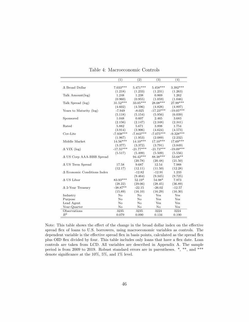
Table 4: Macroeconomic Controls

(1) (2) (3) (4)

∆ Broad Dollar 7.033*** 5.471*** 5.458*** 3.392***(1.218) (1.233) (1.231) (1.263)

Talk Amount(log) 1.248 1.238 0.869 1.262(0.960) (0.955) (1.059) (1.046)

Talk Spread (log) 31.52*** 33.05*** 28.08*** 27.99***(4.602) (4.596) (4.828) (4.897)

Years to Maturity (log) -7.949 -8.025 -17.23*** -19.05***(5.118) (5.154) (5.956) (6.039)

Sponsored 1.048 0.607 2.465 3.683(2.156) (2.147) (2.348) (2.341)

Rated 5.882 5.671 3.898 1.754(3.914) (3.906) (4.624) (4.573)

Cov-Lite -7.938*** -7.843*** -7.075*** -9.328***(1.967) (1.953) (2.089) (2.232)

Middle Market 14.56*** 14.10*** 17.10*** 17.69***(3.377) (3.372) (3.791) (3.849)

∆ VIX (log) -17.55*** -21.77*** -21.73*** -19.09***(5.517) (5.499) (5.509) (5.556)

∆ US Corp AAA-BBB Spread 94.42*** 88.38*** 53.68**(20.78) (20.48) (21.50)

∆ US Term Spread 17.58 9.687 12.54 7.988(12.17) (12.11) (11.50) (12.28)

∆ Economic Conditions Index -12.82 -12.91 1.233(9.464) (9.345) (9.725)

∆ US Libor 83.93*** 52.19* 54.98* 7.973(28.22) (29.06) (28.45) (36.89)

∆ 2-Year Treasury -38.87** -22.15 -26.02 -12.57(15.89) (16.10) (16.29) (16.30)

Industry No No Yes YesPurpose No No Yes YesLead Agent No No Yes YesYear-Quarter No No No YesObservations 3235 3235 3224 3224R2 0.079 0.090 0.134 0.190

Note: This table shows the effect of the change in the broad dollar index on the effectivespread flex of loans to U.S. borrowers, using macroeconomic variables as controls. Thedependent variable is the effective spread flex in basis points, calculated as the spread flexplus OID flex divided by four. This table includes only loans that have a flex date. Loancontrols are taken from LCD. All variables are described in Appendix A. The sampleperiod is from 2009 to 2019. Robust standard errors are in parentheses. *, **, and ***denote significance at the 10%, 5%, and 1% level.

46

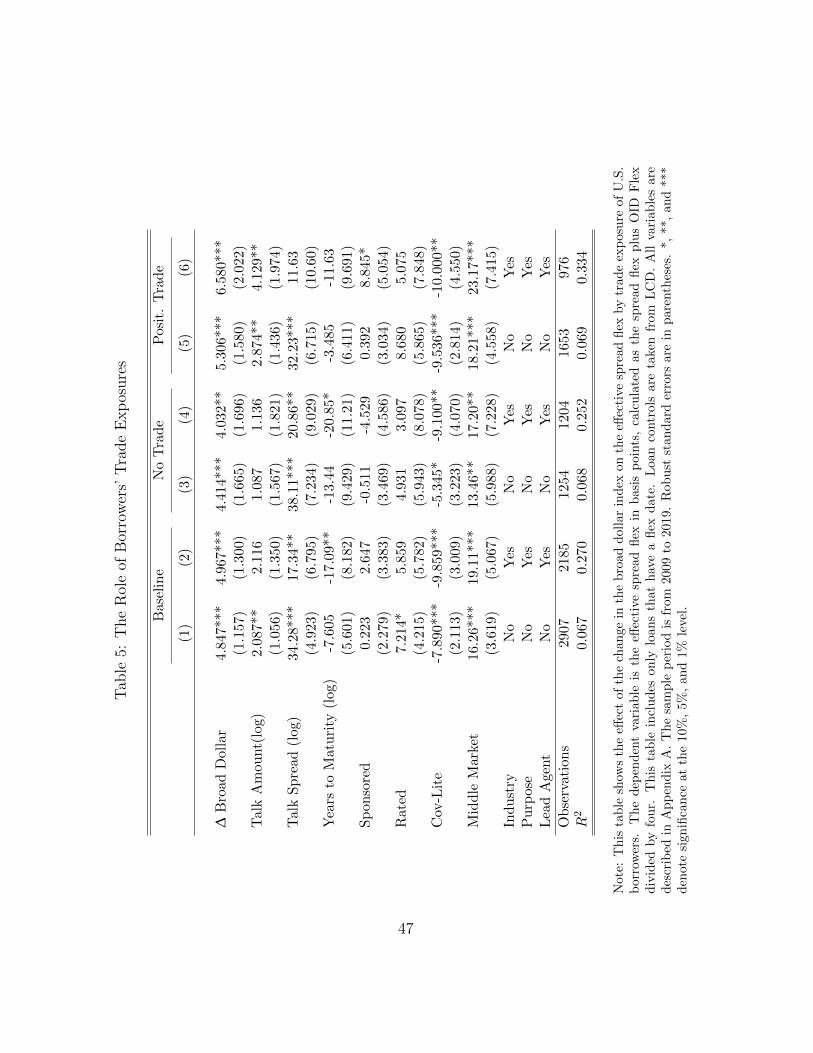
Tab

le5:

The

Rol

eof

Bor

row

ers’

Tra

de

Exp

osure

s

Bas

elin

eN

oT

rad

eP

osit

.T

rad

e

(1)

(2)

(3)

(4)

(5)

(6)

∆B

road

Doll

ar4.

847*

**4.

967*

**4.

414*

**4.

032*

*5.

306*

**6.

580*

**(1

.157

)(1

.300

)(1

.665

)(1

.696

)(1

.580

)(2

.022

)T

alk

Am

ou

nt(

log)

2.08

7**

2.11

61.

087

1.13

62.

874*

*4.

129*

*(1

.056

)(1

.350

)(1

.567

)(1

.821

)(1

.436

)(1

.974

)T

alk

Sp

read

(log

)34

.28*

**17

.34*

*38

.11*

**20

.86*

*32

.23*

**11

.63

(4.9

23)

(6.7

95)

(7.2

34)

(9.0

29)

(6.7

15)

(10.

60)

Yea

rsto

Mat

uri

ty(l

og)

-7.6

05-1

7.09

**-1

3.44

-20.

85*

-3.4

85-1

1.63

(5.6

01)

(8.1

82)

(9.4

29)

(11.

21)

(6.4

11)

(9.6

91)

Sp

on

sore

d0.

223

2.64

7-0

.511

-4.5

290.

392

8.84

5*(2

.279

)(3

.383

)(3

.469

)(4

.586

)(3

.034

)(5

.054

)R

ate

d7.

214*

5.85

94.

931

3.09

78.

680

5.07

5(4

.215

)(5

.782

)(5

.943

)(8

.078

)(5

.865

)(7

.848

)C

ov-L

ite

-7.8

90**

*-9

.859

***

-5.3

45*

-9.1

00**

-9.5

36**

*-1

0.00

0**

(2.1

13)

(3.0

09)

(3.2

23)

(4.0

70)

(2.8

14)

(4.5

50)

Mid

dle

Mar

ket

16.2

6***

19.1

1***

13.4

6**

17.2

0**

18.2

1***

23.1

7***

(3.6

19)

(5.0

67)

(5.9

88)

(7.2

28)

(4.5

58)

(7.4

15)

Ind

ust

ryN

oY

esN

oY

esN

oY

esP

urp

ose

No

Yes

No

Yes

No

Yes

Lea

dA

gen

tN

oY

esN

oY

esN

oY

es

Ob

serv

atio

ns

2907

2185

1254

1204

1653

976

R2

0.06

70.

270

0.06

80.

252

0.06

90.

334

Not

e:T

his

tab

lesh

ows

the

effec

tof

the

chan

gein

the

bro

ad

doll

ar

ind

exon

the

effec

tive

spre

ad

flex

by

trad

eex

posu

reof

U.S

.b

orro

wer

s.T

he

dep

end

ent

vari

able

isth

eeff

ecti

vesp

read

flex

inb

asi

sp

oin

ts,

calc

ula

ted

as

the

spre

ad

flex

plu

sO

IDF

lex

div

ided

by

fou

r.T

his

tab

lein

clu

des

only

loan

sth

at

hav

ea

flex

date

.L

oan

contr

ols

are

take

nfr

om

LC

D.

All

vari

ab

les

are

des

crib

edin

Ap

pen

dix

A.

Th

esa

mp

lep

erio

dis

from

2009

to2019.

Rob

ust

stan

dard

erro

rsare

inp

are

nth

eses

.*,

**,

an

d***

den

ote

sign

ifica

nce

atth

e10

%,

5%,

and

1%le

vel.

47

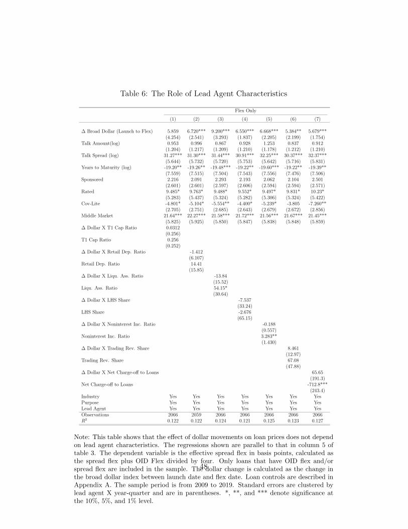
Table 6: The Role of Lead Agent Characteristics

Flex Only

(1) (2) (3) (4) (5) (6) (7)

∆ Broad Dollar (Launch to Flex) 5.859 6.720*** 9.200*** 6.550*** 6.668*** 5.384** 5.679***(4.254) (2.541) (3.293) (1.837) (2.205) (2.199) (1.754)

Talk Amount(log) 0.953 0.996 0.867 0.928 1.253 0.837 0.912(1.204) (1.217) (1.209) (1.210) (1.178) (1.212) (1.210)

Talk Spread (log) 31.27*** 31.30*** 31.44*** 30.91*** 32.25*** 30.37*** 32.37***(5.644) (5.732) (5.720) (5.753) (5.642) (5.716) (5.831)

Years to Maturity (log) -19.20** -19.26** -19.48*** -19.22** -19.60*** -19.22** -19.39**(7.559) (7.515) (7.504) (7.543) (7.556) (7.476) (7.506)

Sponsored 2.216 2.091 2.293 2.193 2.062 2.104 2.501(2.601) (2.601) (2.597) (2.606) (2.594) (2.594) (2.571)

Rated 9.485* 9.763* 9.488* 9.552* 9.497* 9.831* 10.23*(5.283) (5.437) (5.324) (5.282) (5.306) (5.324) (5.422)

Cov-Lite -4.801* -5.104* -5.554** -4.400* -5.239* -3.805 -7.260**(2.705) (2.751) (2.685) (2.643) (2.679) (2.672) (2.856)

Middle Market 21.64*** 22.27*** 21.58*** 21.72*** 21.56*** 21.67*** 21.45***(5.825) (5.925) (5.850) (5.847) (5.838) (5.848) (5.859)

∆ Dollar X T1 Cap Ratio 0.0312(0.256)

T1 Cap Ratio 0.256(0.252)

∆ Dollar X Retail Dep. Ratio -1.412(6.107)

Retail Dep. Ratio 14.41(15.85)

∆ Dollar X Liqu. Ass. Ratio -13.84(15.52)

Liqu. Ass. Ratio 54.15*(30.64)

∆ Dollar X LHS Share -7.537(33.24)

LHS Share -2.676(65.15)

∆ Dollar X Noninterest Inc. Ratio -0.188(0.557)

Noninterest Inc. Ratio 3.283**(1.430)

∆ Dollar X Trading Rev. Share 8.461(12.97)

Trading Rev. Share 67.08(47.88)

∆ Dollar X Net Charge-off to Loans 65.65(191.3)

Net Charge-off to Loans -712.8***(243.4)

Industry Yes Yes Yes Yes Yes Yes YesPurpose Yes Yes Yes Yes Yes Yes YesLead Agent Yes Yes Yes Yes Yes Yes YesObservations 2066 2059 2066 2066 2066 2066 2066R2 0.122 0.122 0.124 0.121 0.125 0.123 0.127

Note: This table shows that the effect of dollar movements on loan prices does not dependon lead agent characteristics. The regressions shown are parallel to that in column 5 oftable 3. The dependent variable is the effective spread flex in basis points, calculated asthe spread flex plus OID Flex divided by four. Only loans that have OID flex and/orspread flex are included in the sample. The dollar change is calculated as the change inthe broad dollar index between launch date and flex date. Loan controls are described inAppendix A. The sample period is from 2009 to 2019. Standard errors are clustered bylead agent X year-quarter and are in parentheses. *, **, and *** denote significance atthe 10%, 5%, and 1% level.

48

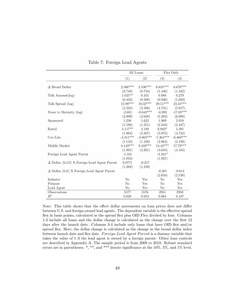
Table 7: Foreign Lead Agents

All Loans Flex Only

(1) (2) (3) (4)

∆ Broad Dollar 2.566*** 2.536*** 6.635*** 6.676***(0.740) (0.734) (1.446) (1.442)

Talk Amount(log) 1.025** 0.455 0.988 0.279(0.433) (0.508) (0.940) (1.050)

Talk Spread (log) 12.99*** 10.32*** 29.51*** 23.24***(2.310) (2.506) (4.741) (5.017)

Years to Maturity (log) -2.681 -8.643*** -6.993 -17.85***(2.009) (2.628) (5.204) (6.098)

Sponsored 1.238 1.622 1.909 2.918(1.186) (1.251) (2.244) (2.447)

Rated 4.117** 3.189 6.802* 5.391(1.963) (2.387) (3.972) (4.742)

Cov-Lite -4.311*** -3.865*** -7.364*** -6.860***(1.110) (1.198) (2.064) (2.199)

Middle Market 8.143*** 9.433*** 14.42*** 17.79***(1.991) (2.261) (3.634) (4.104)

Foreign Lead Agent Parent -1.161 -3.161*(1.053) (1.921)

∆ Dollar (Lt12) X Foreign Lead Agent Parent 0.0771 -0.217(1.269) (1.239)

∆ Dollar (Ltf) X Foreign Lead Agent Parent -0.401 -0.614(2.634) (2.538)

Industry No Yes No YesPurpose No Yes No YesLead Agent No Yes No YesObservations 5577 5576 2951 2950R2 0.028 0.054 0.064 0.107

Note: This table shows that the effect dollar movements on loan prices does not differbetween U.S. and foreign-owned lead agents. The dependent variable is the effective spreadflex in basis points, calculated as the spread flex plus OID Flex divided by four. Columns1-2 include all loans and the dollar change is calculated as the change over the first 12days after the launch date. Columns 3-4 include only loans that have OID flex and/orspread flex. Here, the dollar change is calculated as the change in the broad dollar indexbetween launch date and flex date. Foreign Lead Agent Parent is a dummy variable thattakes the value of 1 if the lead agent is owned by a foreign parent. Other loan controlsare described in Appendix A. The sample period is from 2009 to 2019. Robust standarderrors are in parentheses. *, **, and *** denote significance at the 10%, 5%, and 1% level.

49

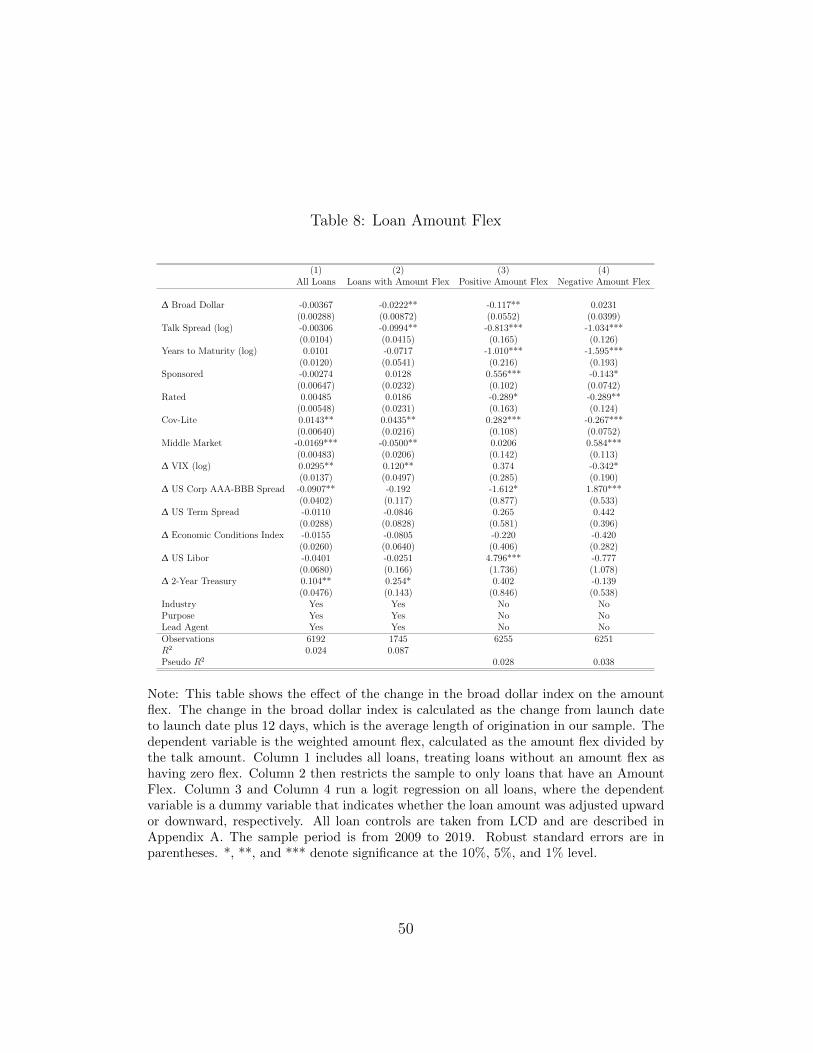
Table 8: Loan Amount Flex

(1) (2) (3) (4)All Loans Loans with Amount Flex Positive Amount Flex Negative Amount Flex

∆ Broad Dollar -0.00367 -0.0222** -0.117** 0.0231(0.00288) (0.00872) (0.0552) (0.0399)

Talk Spread (log) -0.00306 -0.0994** -0.813*** -1.034***(0.0104) (0.0415) (0.165) (0.126)

Years to Maturity (log) 0.0101 -0.0717 -1.010*** -1.595***(0.0120) (0.0541) (0.216) (0.193)

Sponsored -0.00274 0.0128 0.556*** -0.143*(0.00647) (0.0232) (0.102) (0.0742)

Rated 0.00485 0.0186 -0.289* -0.289**(0.00548) (0.0231) (0.163) (0.124)

Cov-Lite 0.0143** 0.0435** 0.282*** -0.267***(0.00640) (0.0216) (0.108) (0.0752)

Middle Market -0.0169*** -0.0500** 0.0206 0.584***(0.00483) (0.0206) (0.142) (0.113)

∆ VIX (log) 0.0295** 0.120** 0.374 -0.342*(0.0137) (0.0497) (0.285) (0.190)

∆ US Corp AAA-BBB Spread -0.0907** -0.192 -1.612* 1.870***(0.0402) (0.117) (0.877) (0.533)

∆ US Term Spread -0.0110 -0.0846 0.265 0.442(0.0288) (0.0828) (0.581) (0.396)

∆ Economic Conditions Index -0.0155 -0.0805 -0.220 -0.420(0.0260) (0.0640) (0.406) (0.282)

∆ US Libor -0.0401 -0.0251 4.796*** -0.777(0.0680) (0.166) (1.736) (1.078)

∆ 2-Year Treasury 0.104** 0.254* 0.402 -0.139(0.0476) (0.143) (0.846) (0.538)

Industry Yes Yes No NoPurpose Yes Yes No NoLead Agent Yes Yes No NoObservations 6192 1745 6255 6251R2 0.024 0.087Pseudo R2 0.028 0.038

Note: This table shows the effect of the change in the broad dollar index on the amountflex. The change in the broad dollar index is calculated as the change from launch dateto launch date plus 12 days, which is the average length of origination in our sample. Thedependent variable is the weighted amount flex, calculated as the amount flex divided bythe talk amount. Column 1 includes all loans, treating loans without an amount flex ashaving zero flex. Column 2 then restricts the sample to only loans that have an AmountFlex. Column 3 and Column 4 run a logit regression on all loans, where the dependentvariable is a dummy variable that indicates whether the loan amount was adjusted upwardor downward, respectively. All loan controls are taken from LCD and are described inAppendix A. The sample period is from 2009 to 2019. Robust standard errors are inparentheses. *, **, and *** denote significance at the 10%, 5%, and 1% level.

50

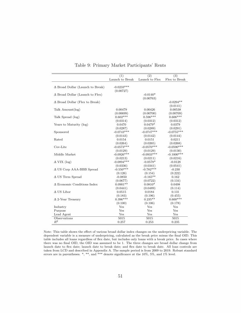
Table 9: Primary Market Participants’ Rents

(1) (2) (3)Launch to Break Launch to Flex Flex to Break

∆ Broad Dollar (Launch to Break) -0.0233***(0.00727)

∆ Broad Dollar (Launch to Flex) -0.0140*(0.00763)

∆ Broad Dollar (Flex to Break) -0.0294**(0.0141)

Talk Amount(log) 0.00479 0.00426 0.00538(0.00699) (0.00700) (0.00709)

Talk Spread (log) 0.602*** 0.596*** 0.606***(0.0314) (0.0312) (0.0312)

Years to Maturity (log) 0.0470 0.0479* 0.0379(0.0287) (0.0289) (0.0291)

Sponsored -0.0743*** -0.0747*** -0.0755***(0.0143) (0.0142) (0.0144)

Rated 0.0154 0.0151 0.0211(0.0264) (0.0265) (0.0268)

Cov-Lite -0.0573*** -0.0570*** -0.0590***(0.0129) (0.0129) (0.0130)

Middle Market -0.0926*** -0.0933*** -0.1000***(0.0213) (0.0211) (0.0216)

∆ VIX (log) -0.0894*** -0.0578* -0.0128(0.0336) (0.0341) (0.0541)

∆ US Corp AAA-BBB Spread -0.550*** -0.782*** -0.230(0.126) (0.154) (0.222)

∆ US Term Spread -0.0850 -0.165** 0.162(0.0677) (0.0722) (0.134)

∆ Economic Conditions Index 0.0901** 0.0810* 0.0498(0.0441) (0.0489) (0.114)

∆ US Libor 0.0515 0.0184 0.131(0.183) (0.196) (0.455)

∆ 2-Year Treasury 0.396*** 0.235** 0.600***(0.100) (0.106) (0.178)

Industry Yes Yes YesPurpose Yes Yes YesLead Agent Yes Yes YesObservations 5015 5015 5015R2 0.257 0.253 0.235

Note: This table shows the effect of various broad dollar index changes on the underpricing variable. Thedependent variable is a measure of underpricing, calculated as the break price minus the final OID. Thistable includes all loans regardless of flex date, but includes only loans with a break price. In cases wherethere was no final OID, the OID was assumed to be 1. The three changes are broad dollar change fromlaunch date to flex date; launch date to break date; and flex date to break date. All loan controls aretaken from LCD and described in Appendix A. The sample period is from 2009 to 2019. Robust standarderrors are in parentheses. *, **, and *** denote significance at the 10%, 5%, and 1% level.

51

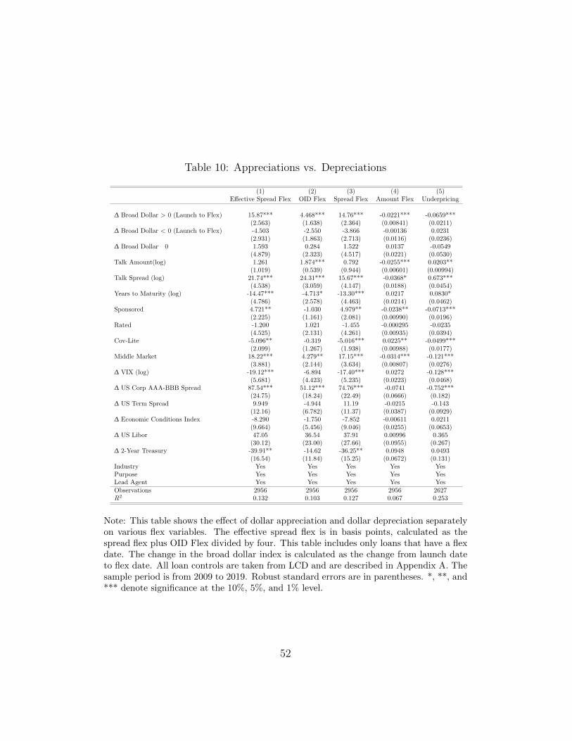
Table 10: Appreciations vs. Depreciations

(1) (2) (3) (4) (5)Effective Spread Flex OID Flex Spread Flex Amount Flex Underpricing

∆ Broad Dollar > 0 (Launch to Flex) 15.87*** 4.468*** 14.76*** -0.0221*** -0.0659***(2.563) (1.638) (2.364) (0.00841) (0.0211)

∆ Broad Dollar < 0 (Launch to Flex) -4.503 -2.550 -3.866 -0.00136 0.0231(2.931) (1.863) (2.713) (0.0116) (0.0236)

∆ Broad Dollar 0 1.593 0.284 1.522 0.0137 -0.0549(4.879) (2.323) (4.517) (0.0221) (0.0530)

Talk Amount(log) 1.261 1.874*** 0.792 -0.0255*** 0.0203**(1.019) (0.539) (0.944) (0.00601) (0.00994)

Talk Spread (log) 21.74*** 24.31*** 15.67*** -0.0368* 0.673***(4.538) (3.059) (4.147) (0.0188) (0.0454)

Years to Maturity (log) -14.47*** -4.713* -13.30*** 0.0217 0.0830*(4.786) (2.578) (4.463) (0.0214) (0.0462)

Sponsored 4.721** -1.030 4.979** -0.0238** -0.0713***(2.225) (1.161) (2.081) (0.00990) (0.0196)

Rated -1.200 1.021 -1.455 -0.000295 -0.0235(4.525) (2.131) (4.261) (0.00935) (0.0394)

Cov-Lite -5.096** -0.319 -5.016*** 0.0225** -0.0499***(2.099) (1.267) (1.938) (0.00988) (0.0177)

Middle Market 18.22*** 4.279** 17.15*** -0.0314*** -0.121***(3.881) (2.144) (3.634) (0.00807) (0.0276)

∆ VIX (log) -19.12*** -6.894 -17.40*** 0.0272 -0.128***(5.681) (4.423) (5.235) (0.0223) (0.0468)

∆ US Corp AAA-BBB Spread 87.54*** 51.12*** 74.76*** -0.0741 -0.752***(24.75) (18.24) (22.49) (0.0666) (0.182)

∆ US Term Spread 9.949 -4.944 11.19 -0.0215 -0.143(12.16) (6.782) (11.37) (0.0387) (0.0929)

∆ Economic Conditions Index -8.290 -1.750 -7.852 -0.00611 0.0211(9.664) (5.456) (9.046) (0.0255) (0.0653)

∆ US Libor 47.05 36.54 37.91 0.00996 0.365(30.12) (23.00) (27.66) (0.0955) (0.267)

∆ 2-Year Treasury -39.91** -14.62 -36.25** 0.0948 0.0493(16.54) (11.84) (15.25) (0.0672) (0.131)

Industry Yes Yes Yes Yes YesPurpose Yes Yes Yes Yes YesLead Agent Yes Yes Yes Yes YesObservations 2956 2956 2956 2956 2627R2 0.132 0.103 0.127 0.067 0.253

Note: This table shows the effect of dollar appreciation and dollar depreciation separatelyon various flex variables. The effective spread flex is in basis points, calculated as thespread flex plus OID Flex divided by four. This table includes only loans that have a flexdate. The change in the broad dollar index is calculated as the change from launch dateto flex date. All loan controls are taken from LCD and are described in Appendix A. Thesample period is from 2009 to 2019. Robust standard errors are in parentheses. *, **, and*** denote significance at the 10%, 5%, and 1% level.

52

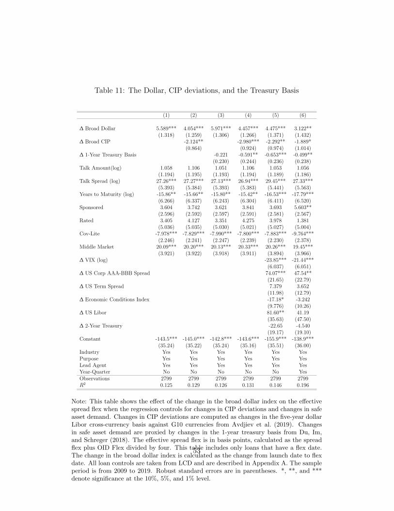
Table 11: The Dollar, CIP deviations, and the Treasury Basis

(1) (2) (3) (4) (5) (6)

∆ Broad Dollar 5.589*** 4.054*** 5.971*** 4.457*** 4.475*** 3.122**(1.318) (1.259) (1.306) (1.266) (1.371) (1.432)

∆ Broad CIP -2.124** -2.980*** -2.292** -1.889*(0.864) (0.924) (0.974) (1.014)

∆ 1-Year Treasury Basis -0.221 -0.591** -0.653*** -0.499**(0.230) (0.244) (0.236) (0.238)

Talk Amount(log) 1.058 1.106 1.051 1.106 1.053 1.056(1.194) (1.195) (1.193) (1.194) (1.189) (1.186)

Talk Spread (log) 27.26*** 27.27*** 27.13*** 26.94*** 29.45*** 27.33***(5.393) (5.384) (5.393) (5.383) (5.441) (5.563)

Years to Maturity (log) -15.86** -15.66** -15.80** -15.42** -16.53*** -17.79***(6.266) (6.337) (6.243) (6.304) (6.411) (6.520)

Sponsored 3.604 3.742 3.621 3.841 3.693 5.603**(2.596) (2.592) (2.597) (2.591) (2.581) (2.567)

Rated 3.405 4.127 3.351 4.275 3.978 1.381(5.036) (5.035) (5.030) (5.021) (5.027) (5.004)

Cov-Lite -7.978*** -7.829*** -7.990*** -7.800*** -7.883*** -9.764***(2.246) (2.241) (2.247) (2.239) (2.230) (2.378)

Middle Market 20.09*** 20.20*** 20.13*** 20.33*** 20.26*** 19.45***(3.921) (3.922) (3.918) (3.911) (3.894) (3.966)

∆ VIX (log) -23.85*** -21.44***(6.037) (6.051)

∆ US Corp AAA-BBB Spread 74.07*** 47.54**(21.65) (22.79)

∆ US Term Spread 7.379 3.652(11.98) (12.79)

∆ Economic Conditions Index -17.18* -3.242(9.776) (10.26)

∆ US Libor 81.60** 41.19(35.63) (47.50)

∆ 2-Year Treasury -22.65 -4.540(19.17) (19.10)

Constant -143.5*** -145.0*** -142.8*** -143.6*** -155.9*** -138.9***(35.24) (35.22) (35.24) (35.16) (35.51) (36.00)

Industry Yes Yes Yes Yes Yes YesPurpose Yes Yes Yes Yes Yes YesLead Agent Yes Yes Yes Yes Yes YesYear-Quarter No No No No No YesObservations 2799 2799 2799 2799 2799 2799R2 0.125 0.129 0.126 0.131 0.146 0.196

Note: This table shows the effect of the change in the broad dollar index on the effectivespread flex when the regression controls for changes in CIP deviations and changes in safeasset demand. Changes in CIP deviations are computed as changes in the five-year dollarLibor cross-currency basis against G10 currencies from Avdjiev et al. (2019). Changesin safe asset demand are proxied by changes in the 1-year treasury basis from Du, Im,and Schreger (2018). The effective spread flex is in basis points, calculated as the spreadflex plus OID Flex divided by four. This table includes only loans that have a flex date.The change in the broad dollar index is calculated as the change from launch date to flexdate. All loan controls are taken from LCD and are described in Appendix A. The sampleperiod is from 2009 to 2019. Robust standard errors are in parentheses. *, **, and ***denote significance at the 10%, 5%, and 1% level.

53

Internet Appendix

A Data

The appendix provides the definitions of all variables used in the empirical analysisand presents additional data summary statistics.

Table A1 gives detailed variables definitions and sources for each variable usedin our analysis.

Figure A1 shows the ratings distribution of the loans in our sample.Figure A2 shows the time series of the changes in the dollar and changes in US

high-yield spreads.

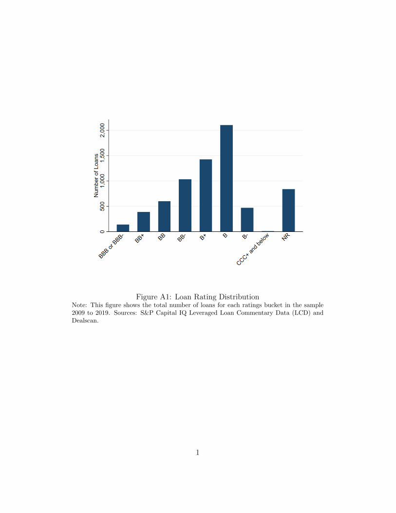
Figure A1: Loan Rating DistributionNote: This figure shows the total number of loans for each ratings bucket in the sample2009 to 2019. Sources: S&P Capital IQ Leveraged Loan Commentary Data (LCD) andDealscan.

1

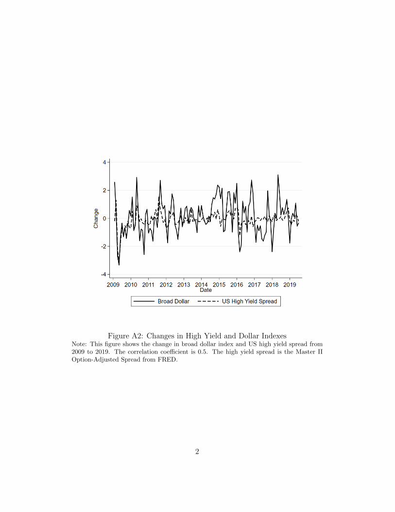
Figure A2: Changes in High Yield and Dollar IndexesNote: This figure shows the change in broad dollar index and US high yield spread from2009 to 2019. The correlation coefficient is 0.5. The high yield spread is the Master IIOption-Adjusted Spread from FRED.

2

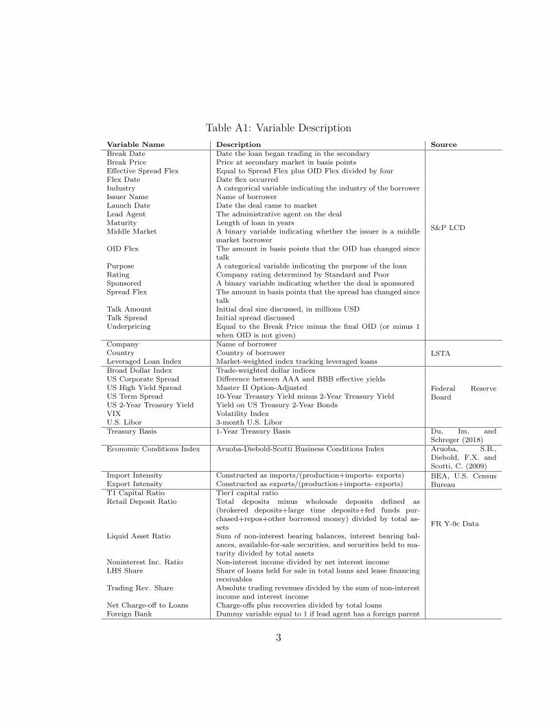
Table A1: Variable Description

Variable Name Description SourceBreak Date Date the loan began trading in the secondary

S&P LCD

Break Price Price at secondary market in basis pointsEffective Spread Flex Equal to Spread Flex plus OID Flex divided by fourFlex Date Date flex occurredIndustry A categorical variable indicating the industry of the borrowerIssuer Name Name of borrowerLaunch Date Date the deal came to marketLead Agent The administrative agent on the dealMaturity Length of loan in yearsMiddle Market A binary variable indicating whether the issuer is a middle

market borrowerOID Flex The amount in basis points that the OID has changed since

talkPurpose A categorical variable indicating the purpose of the loanRating Company rating determined by Standard and PoorSponsored A binary variable indicating whether the deal is sponsoredSpread Flex The amount in basis points that the spread has changed since

talkTalk Amount Initial deal size discussed, in millions USDTalk Spread Initial spread discussedUnderpricing Equal to the Break Price minus the final OID (or minus 1

when OID is not given)Company Name of borrower

LSTACountry Country of borrowerLeveraged Loan Index Market-weighted index tracking leveraged loansBroad Dollar Index Trade-weighted dollar indices

Federal ReserveBoard

US Corporate Spread Difference between AAA and BBB effective yieldsUS High Yield Spread Master II Option-AdjustedUS Term Spread 10-Year Treasury Yield minus 2-Year Treasury YieldUS 2-Year Treasury Yield Yield on US Treasury 2-Year BondsVIX Volatility IndexU.S. Libor 3-month U.S. LiborTreasury Basis 1-Year Treasury Basis Du, Im, and

Schreger (2018)

Economic Conditions Index Aruoba-Diebold-Scotti Business Conditions Index Aruoba, S.B.,Diebold, F.X. andScotti, C. (2009)

Import Intensity Constructed as imports/(production+imports- exports) BEA, U.S. CensusBureauExport Intensity Constructed as exports/(production+imports- exports)

T1 Capital Ratio Tier1 capital ratio

FR Y-9c Data

Retail Deposit Ratio Total deposits minus wholesale deposits defined as(brokered deposits+large time deposits+fed funds pur-chased+repos+other borrowed money) divided by total as-sets

Liquid Asset Ratio Sum of non-interest bearing balances, interest bearing bal-ances, available-for-sale securities, and securities held to ma-turity divided by total assets

Noninterest Inc. Ratio Non-interest income divided by net interest incomeLHS Share Share of loans held for sale in total loans and lease financing

receivablesTrading Rev. Share Absolute trading revenues divided by the sum of non-interest

income and interest incomeNet Charge-off to Loans Charge-offs plus recoveries divided by total loansForeign Bank Dummy variable equal to 1 if lead agent has a foreign parent

3

B Robustness Tests

U.S. vs Non-U.S. BorrowersWe now study whether the effect of movements in the dollar index differ for U.S.

and non-U.S. corporate borrowers. Non-U.S. corporate borrowers’ ability to repayU.S. dollar denominated loans may decrease if most of the revenues are in localcurrency, directly linking credit risk and dollar movements.46 That said, if theeffects of dollar movements on borrowing cost for U.S. and non-U.S. corporationsare similar, this would suggest that movements in the dollar index reflect changesin global risk appetite and the global demand for risky assets that are transmittedto borrowers through higher spreads.

Table B1 shows the results of estimating equation 2 separately for U.S. andnon-U.S. borrowers. Comparing the results for U.S. corporations without andwith macroeconomic controls (columns 1 and 2) to the corresponding results fornon-U.S. corporations (columns 3 and 4) shows that the effects are sizable andstatistically significant. The effects of dollar movements on spreads for non-U.S.corporations are somewhat larger than for U.S. corporations, potentially reflectingthe fact that the loans are denominated in U.S. dollars exposing non-U.S. borrowersto exchange rate risk. However, the differences in the dollar coefficient betweenU.S. and non-U.S. borrowers are not statistically significant (columns 5 and 6).

Explanatory power of key risk proxies when the dollar is omittedTo clarify the explanatory power of key variables that proxy for risk and un-

certainty, we exclude the dollar from the effective spread flex regression in tableB2.

Columns 1 and 2 show the result of estimating our main specification withchanges in the 1-Year Treasury basis over the syndication period as main explana-tory variable. We find no effect of changes in the 1-Year Treasury basis on changesin the loan spread. We then explore the effect of changes in uncertainty, measuredas changes in the VIX. Columns 3 and 4 show the results of estimating our mainspecification with the changes in the VIX over the syndication period as mainexplanatory variable. We find no effect of changes in the VIX on loan spreadchanges. Taken together, these result suggest that neither scarcity of dollar safeassets or uncertainty explain the effective spread flex per se.

Columns 5 and 6 show that the U.S. yield spread is significantly positively cor-related with the effective spread flex when changes in the dollar index are omittedas control variable. The coefficient increases compared to the results in earliertables with change in the dollar included, as one might have expected because

46It is common, however, that loan agreements mandate corporation hedge exchangerate risk, partially alleviating this concern.

4

changes in the high yield spread and the dollar a highly correlated. Similarly,columns 7 and 8 indicate that changes in CIP deviations have a statistically signif-icant effect on the effective spread flex when changes in the dollar are not controlledfor. Omitting changes in the dollar increases the coefficient also in this case asexpected.

5

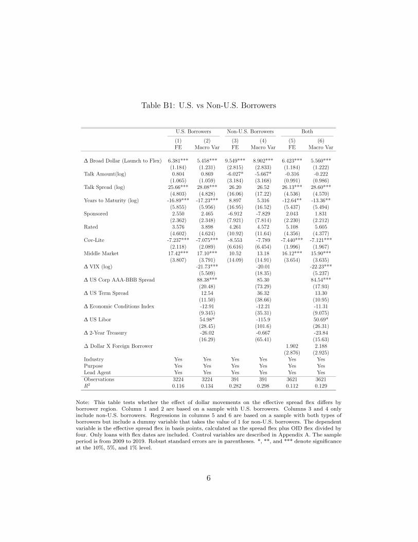
Table B1: U.S. vs Non-U.S. Borrowers

U.S. Borrowers Non-U.S. Borrowers Both

(1) (2) (3) (4) (5) (6)FE Macro Var FE Macro Var FE Macro Var

∆ Broad Dollar (Launch to Flex) 6.381*** 5.458*** 9.549*** 8.902*** 6.423*** 5.560***(1.184) (1.231) (2.815) (2.833) (1.184) (1.222)

Talk Amount(log) 0.804 0.869 -6.027* -5.667* -0.316 -0.222(1.065) (1.059) (3.184) (3.168) (0.991) (0.986)

Talk Spread (log) 25.66*** 28.08*** 26.20 26.52 26.13*** 28.60***(4.803) (4.828) (16.06) (17.22) (4.536) (4.570)

Years to Maturity (log) -16.89*** -17.23*** 8.897 5.316 -12.64** -13.36**(5.855) (5.956) (16.95) (16.52) (5.437) (5.494)

Sponsored 2.550 2.465 -6.912 -7.829 2.043 1.831(2.362) (2.348) (7.921) (7.814) (2.230) (2.212)

Rated 3.576 3.898 4.261 4.572 5.108 5.605(4.602) (4.624) (10.92) (11.64) (4.356) (4.377)

Cov-Lite -7.237*** -7.075*** -8.553 -7.789 -7.440*** -7.121***(2.118) (2.089) (6.616) (6.454) (1.996) (1.967)

Middle Market 17.42*** 17.10*** 10.52 13.18 16.12*** 15.90***(3.807) (3.791) (14.09) (14.91) (3.654) (3.635)

∆ VIX (log) -21.73*** -20.01 -22.23***(5.509) (18.35) (5.237)

∆ US Corp AAA-BBB Spread 88.38*** 85.30 84.54***(20.48) (73.29) (17.93)

∆ US Term Spread 12.54 36.32 13.30(11.50) (38.66) (10.95)

∆ Economic Conditions Index -12.91 -12.21 -11.31(9.345) (35.31) (9.075)

∆ US Libor 54.98* -115.9 50.69*(28.45) (101.6) (26.31)

∆ 2-Year Treasury -26.02 -0.667 -23.84(16.29) (65.41) (15.63)

∆ Dollar X Foreign Borrower 1.902 2.188(2.876) (2.925)

Industry Yes Yes Yes Yes Yes YesPurpose Yes Yes Yes Yes Yes YesLead Agent Yes Yes Yes Yes Yes YesObservations 3224 3224 391 391 3621 3621R2 0.116 0.134 0.282 0.298 0.112 0.129

Note: This table tests whether the effect of dollar movements on the effective spread flex differs byborrower region. Column 1 and 2 are based on a sample with U.S. borrowers. Columns 3 and 4 onlyinclude non-U.S. borrowers. Regressions in columns 5 and 6 are based on a sample with both types ofborrowers but include a dummy variable that takes the value of 1 for non-U.S. borrowers. The dependentvariable is the effective spread flex in basis points, calculated as the spread flex plus OID flex divided byfour. Only loans with flex dates are included. Control variables are described in Appendix A. The sampleperiod is from 2009 to 2019. Robust standard errors are in parentheses. *, **, and *** denote significanceat the 10%, 5%, and 1% level.

6

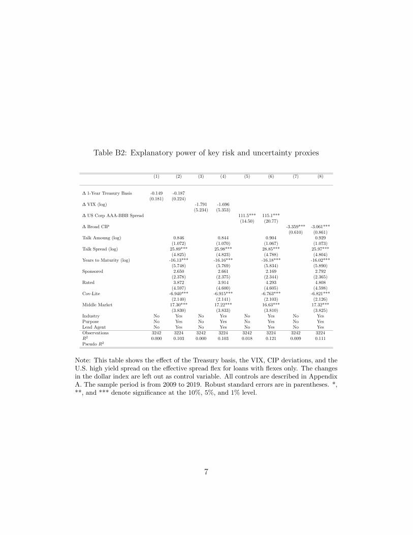
Table B2: Explanatory power of key risk and uncertainty proxies

(1) (2) (3) (4) (5) (6) (7) (8)

∆ 1-Year Treasury Basis -0.149 -0.187(0.181) (0.224)

∆ VIX (log) -1.791 -1.696(5.234) (5.353)

∆ US Corp AAA-BBB Spread 111.5*** 115.1***(14.50) (20.77)

∆ Broad CIP -3.359*** -3.061***(0.610) (0.861)

Talk Amoung (log) 0.846 0.844 0.904 0.929(1.072) (1.070) (1.067) (1.073)

Talk Spread (log) 25.89*** 25.98*** 28.85*** 25.97***(4.825) (4.823) (4.788) (4.804)

Years to Maturity (log) -16.13*** -16.16*** -16.18*** -16.02***(5.748) (5.769) (5.834) (5.890)

Sponsored 2.650 2.661 2.169 2.792(2.378) (2.375) (2.344) (2.365)

Rated 3.872 3.914 4.293 4.808(4.597) (4.600) (4.605) (4.598)

Cov-Lite -6.940*** -6.915*** -6.763*** -6.821***(2.140) (2.141) (2.103) (2.126)

Middle Market 17.30*** 17.22*** 16.63*** 17.32***(3.830) (3.833) (3.810) (3.825)

Industry No Yes No Yes No Yes No YesPurpose No Yes No Yes No Yes No YesLead Agent No Yes No Yes No Yes No YesObservations 3242 3224 3242 3224 3242 3224 3242 3224R2 0.000 0.103 0.000 0.103 0.018 0.121 0.009 0.111Pseudo R2

Note: This table shows the effect of the Treasury basis, the VIX, CIP deviations, and theU.S. high yield spread on the effective spread flex for loans with flexes only. The changesin the dollar index are left out as control variable. All controls are described in AppendixA. The sample period is from 2009 to 2019. Robust standard errors are in parentheses. *,**, and *** denote significance at the 10%, 5%, and 1% level.

7

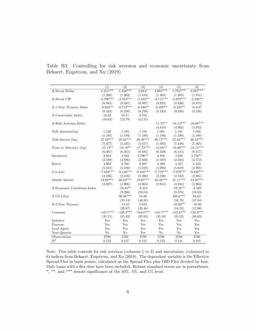
Table B3: Controlling for risk aversion and economic uncertainty fromBekaert, Engstrom, and Xu (2019)

(1) (2) (3) (4) (5) (6)∆ Broad Dollar 4.314*** 4.459*** 2.684* 4.984*** 5.752*** 3.887***

(1.266) (1.363) (1.410) (1.304) (1.403) (1.451)∆ Broad CIP -2.706*** -2.854*** -2.163** -3.115*** -2.979*** -2.328**

(0.945) (0.947) (0.987) (0.924) (0.938) (0.975)∆ 1-Year Treasury Basis -0.624** -0.713*** -0.530** -0.498** -0.594** -0.413*

(0.242) (0.238) (0.239) (0.243) (0.238) (0.238)∆ Uncertainty Index 16.22 10.11 3.705

(10.63) (12.79) (12.55)∆ Risk Aversion Index -11.75** -16.13*** -16.68***

(4.810) (4.992) (4.972)Talk Amount(log) 1.129 1.194 1.180 1.001 1.101 1.058

(1.195) (1.194) (1.190) (1.190) (1.190) (1.188)Talk Spread (log) 27.22*** 28.04*** 26.38*** 26.77*** 27.64*** 26.53***

(5.377) (5.435) (5.557) (5.383) (5.448) (5.565)Years to Maturity (log) -15.13** -16.19** -17.73*** -15.69** -16.86*** -18.11***

(6.301) (6.355) (6.485) (6.329) (6.415) (6.517)Sponsored 3.924 4.032 5.790** 3.856 4.050 5.750**

(2.588) (2.586) (2.568) (2.595) (2.594) (2.572)Rated 4.062 3.700 0.887 4.398 4.167 1.453

(5.024) (5.038) (5.018) (4.998) (5.018) (4.995)Cov-Lite -7.838*** -8.146*** -9.948*** -7.719*** -7.979*** -9.836***

(2.236) (2.249) (2.386) (2.238) (2.242) (2.381)Middle Market 19.99*** 20.82*** 19.65*** 20.49*** 21.11*** 19.76***

(3.897) (3.906) (3.963) (3.914) (3.910) (3.963)∆ Economic Conditions Index -19.85** -3.224 -19.25** -2.569

(9.398) (10.04) (9.376) (10.03)∆ US Libor 96.86*** 55.80 109.6*** 64.63

(35.14) (46.95) (34.79) (47.04)∆ 2-Year Treasury -15.81 5.023 -42.00** -16.92

(20.87) (20.46) (18.52) (17.98)Constant -145.7*** -149.3*** -134.0*** -141.7*** -145.6*** -133.9***

(35.15) (35.42) (35.95) (35.16) (35.52) (36.03)Industry Yes Yes Yes Yes Yes YesPurpose Yes Yes Yes Yes Yes YesLead Agent Yes Yes Yes Yes Yes YesYear-Quarter No No Yes No No YesObservations 2799 2799 2799 2799 2799 2799R2 0.132 0.137 0.191 0.133 0.141 0.195

Note: This table controls for risk aversion (columns 1 to 3) and uncertainty (columns4 to6) indices from Bekaert, Engstrom, and Xu (2019). The dependent variable is the EffectiveSpread Flex in basis points, calculated as the Spread Flex plus OID Flex divided by four.Only loans with a flex date have been included. Robust standard errors are in parentheses.*, **, and *** denote significance at the 10%, 5%, and 1% level.

8

Documents

The Dollar and Corporate Borrowing Costs