The Distribution of Treatment Effects in Experimental Settings:Applications of Nonlinear Difference-in-Difference Approaches

Susan Athey - Stanford

Guido W. Imbens - UC Berkeley

1

Introduction

• Based on: “Identification and Inference in Nonlinear Difference-in-Differences Models” with Guido Imbens, forthcoming in EMA

• Ideas and Themes for Practice— Heterogeneous effects (remain in presence of randomization)

— Focus on distributions of outcomes

∗ Counterfactual dist’ns of what would have happened in ab-sense of treatment, in presence of treatment

∗ Use all of the information in the data, e.g. 4 dist’ns— Economic v. functional form assumptions

∗ Identification v. estimation— Verifying assumptions

∗What are crucial assns and what are convenient?∗ Are “standard” checks, e.g. group similarity on obs., mostimpt.?

• Questions our approach will address:—What is distribution of effects of TOT and TOC?

∗ How do they differ? Optimal policy adoption?—Which individuals are affected?

—Why quantile regression does not make sense in many apps

2

Basic Setup: 2 × 2 Case

• Four subpopulations• “Rows” and “Columns”: Groups and time periods

Group A Group B

Time 2 Treated

Time 1

3

Examples: Overview

• State Policy Change— 2 states, 2 time pds, law changes in one state in 2nd pd

— Groups are different

—Worried about time trend

— Ex: Minimumwage (Card-Krueger), Disability benefits (Meyer-

Viscusi-Durbin)

• Experiment with Heterogeneous Subjects— 2 groups, 2 treatments, 2nd treatment has differential impact

— Groups are different (and heterogeneity w/i group)

— Interested in group difference relative to difference in baseline

treatment

— Examples:

∗ Lab experiment: men and women, 1st treatment measuresability, 2nd treatment tournament

∗ Auction identical items on eBay and Amazon, vary auctionconditions

• Dynamics and Learning in the Lab— Control and treatment group, dynamic game or learning

— Use initial play to learn about intrinsic differences in two

games

— See how differences evolve over time

4

• Hospital Technology Adoption Field Experiment— Two hospitals, two time periods, one adopts surgical tech in

2nd pd

— Hospitals are different

— Patients randomly assigned in each pd

— Pre-surgical technology changes over time

• Effects of Training/Experience on Ability Tests— Subjects take a test to measure ability

— Randomly assigned to different tests

— Randomly assigned to training (or to practice test)

— Does training/experience have different distn of benefits for

different tests?

5

Formal Model

• 2 × 2 case• N observations on (Y, T,G)

• Y is outcome• T ∈ {1, 2} is time period,• G ∈ {A,B} is group.• Group G = B in period T = 2 is the only group/period exposedto intervention.

— Y I is outcome if treated; observed if G = B, T = 2

— Y N is outcome if untreated; observed unless G = B, T = 2

• Let Ygt be r.v. with dist’n of Y |G = g, T = t.

6

Standard DID Model

• Model for outcome in absence of intervention:Y N = α + β · T + η ·G + ε,

with

ε ⊥ (T,G).

—Weaker assn: mean-indep

• Average outcome for subpop (B, 2) in absence of intervention:E[Y NB2] = α + β + η

= E[YB1] + [E[YA2]− E[YA1]]

• Average treatment effect on treated group:τDID = E[Y IB2]− E[Y NB2]

= E[YB2]− E[YB1]− [E[YA2]− E[YA1]]— Note: no model required for Y IB2

7

Fitting Example Into Standard DID Model: State-level

Policy Adoption

• States choose whether to adopt health program— State A has more sick people than State B

— Program more effective on sicker patients

∗ State B adopts in response to voter demand & cost-benefitanalysis

— Hospital outcomes observed

— Medical treatments change each year

∗ Benefit sickest patients most∗ Expect average time trend to differ across counties in ab-sence of program

• Standard model doesn’t apply• Questions our approach will address:—What was benefit to State B?

—What would the benefit be to State A?

—Which patients helped most?

8

Summary of Problems with Standard DID Model

We will address:

• Linearity/additivity— Rules out interesting economics

∗ Cannot have effect of unobservable change over time, mean-variance shift over time

— Assumption not invariant to transformation of dep. variable

• Get effect of the treatment on the treated, not control— Leads to constant treatment effect assn’s or assn of “exoge-

nous” policy adoption

• Problems with binary/discrete outcomes— Linear model can predict outcomes out of bounds

We will ignore:

• Treatment affects group comp. (Heckman 1996; Marrufo 2001)• Issues with standard errors (Donald and Lang, 2001; Bertrand,Duflo, and Mullainathan, 2001)

9

Our Baseline Model: “Changes-in-Changes”

A0 (Model) Y N = h(U, T ).

• h is nonlinear, unknown function— “Production function” does not vary with group

— All diff’s across groups due to dist’n of U

A1 (Time Invariance) U ⊥ T | G.

• Group composition does not change over time— Ex: state or county, short time periods

A2 (Monotonicity) h(u, t) is strictly montone in u.

• Not a restriction in a single period— Restrictive in conjunction with (A1)

— Enables inference of change in prod fn over time

• Std model has two add’l restrictions:U = η ·G + ε

h(U, T ) = α + β · T + U— Note: No assn’s (yet) on effect of treatment. Focus first on

treatment on treated.

10

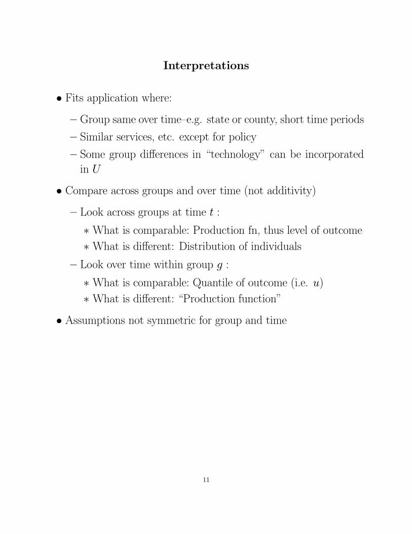
Interpretations

• Fits application where:— Group same over time—e.g. state or county, short time periods

— Similar services, etc. except for policy

— Some group differences in “technology” can be incorporated

in U

• Compare across groups and over time (not additivity)— Look across groups at time t :

∗What is comparable: Production fn, thus level of outcome∗What is different: Distribution of individuals

— Look over time within group g :

∗What is comparable: Quantile of outcome (i.e. u)∗What is different: “Production function”

• Assumptions not symmetric for group and time

11

Fitting Example into CIC Model: State Policy Change

• Economic assns— States differ in distn of unobs factors affecting health U :

policy assignment NOT “random”

— (A1) Groups stable over time: distn of U does not vary w/i

group

— Mapping from U to outcomes, hN(U, t) and hI(U, t) are (A2)

monotone and depend on (i) time (t) and (ii) treatment status,

but (A0) not directly on group

• Interpreting (A2) and (A3):— Pd. 1: health outcome hN(U, 1) ≡ U∗ Incorporates some differences in infrastructure, etc.

— Pd. 2: hN(U, 2) 6= U due to changes in health technology thatapply to both treatment and control group and do not change

ranking of outcomes

— w/o treatment, mapping from unobs to outcomes same in both

states due to similar technology changes

12

Identification of (Continuous) CIC Model

Theorem 1 Assume:

(i) CIC model: A0-A2,

(ii) supp[YB1] ⊆supp[YA1].Then the distribution of Y NB2 is identified and given by

FY N ,B2(y) = FY,B1(F−1Y,A1(FY,A2(y))).

See paper for nonparametric estimation, CAN, efficiency.

“Proof”

• Pick a first period treated unit with outcome y.• Find someone with the same outcome y in the first period controlgroup. By the model these units must have the same unobs. u.

• Find the rank of this unit in the (A, 1) distribution, FY,A1(y).• By monotonicity, a control person with the same value of u inperiod 2 would have outcome

F−1Y,A2(FY,A1(y)) = h(h−1(y; 1), 2).

• Apply this transformation to outcome in first period treatmentunit, so that

Pr(Y NB2 ≤ y) = FY,B1¡h(h−1(y; 2), 1)

¢= Pr(F−1Y,A2(FY,A1(YB1)) ≤ y)

= FY,B1(F−1Y,A1(FY,A2(y))).

13

Group 0 Distributions

0

1

-3 -1.5 0 1.5 3Values of Y

Cum

ulat

ive

Dis

trib

utio

n Fu

nctio

n

CDF of Y00

CDF of Y01

y

qq'

Group 1 Distributions

0

1

-3 -1.5 0 1.5 3Values of Y

Cum

ulat

ive

Dis

trib

utio

n Fu

nctio

n

CDF of Y10

CIC Counterfactual CDF of Y11

QDID Counterfactual CDF of Y11

Actual CDF of Y11

y

q

∆QDID

∆CIC

∆CIC

∆QDID

Figure 1: Illustration of Transformations

YA1

YA2

YB1

YB2

YB2YB2

A

B

Interpretation in Terms of Transformation

• Model defines a transformation,kCIC(y) = F−1Y,A2(FY,A1(y)),

such that

Y NB2d∼ kCIC(YB1)

• Standard DID model has simple linear transformation:

kDID(y) = y + E[YA2]− E[YA1].

14

The Effect of the Treatment on the Control Group

• Analogous model assumption:Y I = hI(U, T )

• Goal: Compute distribution of Y IA2.— Problem seems diff’t: only 1/4 subpop’s treated

— But under assn’s, exactly analogous.

• Apply transformation to the time 1, group 1 outcomes:F−1Y I ,B2

(FY,B1(y)) = hI(h−1(y; 1), 2)

so that

Y IA2d∼ F−1

Y I ,B2(FY,B1(YA1))

• End result— Same procedure

— Reverse roles of treatment and control group

15

Fitting Example into CIC Model: Experiment with

Heterogeneous Groups

• See Gneezy, Niederle and Rustichini (2003)• Men and women differ in ability to perform baseline task, definehN(U, 1) = U

• (A1) Groups stable over time: distn of U does not vary w/i group— Same individuals or different cross-sections

• Instead of “treated” and “untreated,” there is a male and femaleproduction function for “treatment” task

— Mapping from U to outcomes, hmale(U, 2) and hfemale(U, 2)

are (A2) monotone

— Treatment task doesn’t cause low-ability individuals to pass

high-ability individuals

• Question: what would distn of female performance be, given un-derlying ability, if they had male production function for treat-

ment task, and vice-vera

— Distn of hmale(U, 2)|female and hfemale(U, 2)|male

16

Fitting Example into CIC Model: Field Experiments

Auctions on eBay and Amazon

• Auction identical objects in different formats• Different sets of bidders at two sites, stable over time, so auctionprice is draw from different distn

• Baseline differences, incorporating different bidders and site dif-ferences: price=hN(U, 1) = U

— All baseline differences accounted for by distn of U varying

across sites

• Compare relative differences from varying auction design param-eters

— Reserve price, buy-it-now, experience rating of seller, etc.

17

The CIC-r Model: Reverse the Roles of Group and

Time Period

• Recall that we make different assumptions for groups and periods• Reverse:— Two groups have identical distributions of unobservables within

a time period (e.g. random assignment)

— Production function stays the same over time in absence of

the treatment

• Result: TOT is identified, apply same formula with roles reversed• TOC not identified w/o extra assumptions— Issue: given that we think groups have different production

functions, not clear what data tells us about production func-

tion of control group in presence of treatment.

18

Example (2): Hospital Technology Adoption Field

Experiment

• Setup— Groups: hospitals Time: before and after CATH

— Group B in period 2 is “treated”

— Patients randomly assigned to hospitals in each period

• Economic assns (imply distn of TOT identified, not TOC)— (A10) Within a period, distn of U same for both hospitals

— Distn of individuals changes over time (new heart drugs avail-

able to patients of both hospitals)

— Hospitals have different production functions

— Mapping fromU to outcomes in absence of treatment, hN(U, g)

is (A2) monotone and depends on hospital (g) but (A00) notdirectly on time

• Ideas— Control hospital tells us how distn of patients changed over

time, use to calculate counterfactual outcomes if hospital pro-

duction function had not changed

— Issue: given that we think hospitals have different production

functions, not clear what data tells us about production func-

tion of control hospital in presence of treatment.

19

The QDID Model: Quantile Regression at Each

Quantile

• Assumptions— Distribution of unobservables same for each subpopulation

∗ Random assignment to variations on treatments∗ Otherwise, why compare quantiles?

— Production function monotone in unobservables

∗ Ranking of outcomes same for all treatment variations— Group effect and time effect are additive

Y = hG(U, g) + hT (U, t) + hI(U)

∗ Imposes testable restrictions on the data∗ Implies average TOT and TOC are the same

• Gives different answer than CIC or CIC-r models• May be applicable in experimental contexts• Our value-added— Unified uderlying structural model motivating regression at

all quantiles

— Test validity

— Generate entire distribution of counterfactual outcomes

20

Conclusions

• Approach— Essence of DID: Control group provides information about

what would have happened to treatment group in the absence

of the treatment

— Data are four distributions

— Use three distributions to predict counterfactual for fourth

∗ Economic assumptions tell you how— Nonparametric structural model, primitives are production

function and distribution of unobservables

— Focus on distributions of effects

• Benefits of Approach— New model relaxes assumptions of standard DID, can be more

or less efficient

— Scale invariance

— No problems with out-of-bounds predictions for discrete vari-

ables

— Treatment can be endogenous to both level of outcome in each

group and anticipated incremental benefit of policy

— Identify effect of treatment on treated and control groups, can

compute structural parameters

— Fewer, but still many, settings where CIC is not applicable

• See paper for discrete outcomes, multiple groups, treatments

21