Embed Size (px)
Citation preview
Model studies of instabilities in heterogeneous materials systems
by
Mark Hyunpong Jhon
A dissertation submitted in partial satisfaction
of the requirements for the degree of
Doctor of Philosophy
in
Engineering-Materials Science and Engineering
in the
GRADUATE DIVISION
of the
UNIVERSITY OF CALIFORNIA, BERKELEY
Committee in charge:
Professor Daryl C. Chrzan, Co-chairProfessor Andreas M. Glaeser, Co-chair
Professor Joel E. MooreProfessor J. W. Morris
Fall 2009
The dissertation of Mark Hyunpong Jhon is approved.
Co-chair Date
Co-chair Date
Date
Date
University of California, BerkeleyFall 2009
Model studies of instabilities in heterogeneous materials systems
Copyright c 2009
by
Mark Hyunpong Jhon
Abstract
Model studies of instabilities in heterogeneous materials systems
by
Mark Hyunpong Jhon
Doctor of Philosophy in Materials Science and Engineering
University of California, Berkeley
Professor Daryl C. Chrzan and Professor Andreas M. Glaeser, Co-chairs
Heterogeneous materials may become structurally unstable under an applied stress. In this thesis,the eects of two dissimilar stresses are studied. First, the methods of statistical mechanics areused to analyze the eects of mechanical stress on the strength of heterogeneous materials. Aphenomenological multi-scale model is presented that analyzes inelastic deformation in a modelnatural composite, nacre. A kinetic Monte Carlo technique is developed to study the mechanicalresponse of the biopolymer. The results of this model are used to generate a cellular automatamodel of the composite material. Under certain conditions, the sizes of plastic events in this modelfollow an apparent power-law distribution. The dynamics are found to be similar to earthquakes,where the slip sizes exhibit a scale-free distribution.
Second, a continuum theory is generated to understand how a model microstructure respondsto thermal stresses. At elevated temperatures, a structure may spontaneously change shape inorder to minimize its overall surface energy. To this end, the stability of a hollow-core dislocationto pearling and coarsening is considered using a linear stability analysis. There is a competitionbetween elastic energy and the anisotropic surface energy. It is shown that suciently small hollow-core dislocations are stable with respect to both forms of structural instability, suggesting a routeto stabilize nanometer-scale wires.
1

For my parents
i
Contents
Contents ii
List of Figures iv
List of Tables vii
Acknowledgements viii
1 Introduction 1
2 Background 4
2.1 Mechanical instabilities in biological composites . . . . . . . . . . . . . . . . . . . . . 4
2.1.1 Mechanical properties of nacre . . . . . . . . . . . . . . . . . . . . . . . . . . 4
2.1.2 Continuum theories . . . . . . . . . . . . . . . . . . . . . . . . . . . . . . . . 5
2.1.3 Statistical mechanics approach . . . . . . . . . . . . . . . . . . . . . . . . . . 8
2.1.4 Summary . . . . . . . . . . . . . . . . . . . . . . . . . . . . . . . . . . . . . . 13
2.2 Capillary instabilities in strained systems . . . . . . . . . . . . . . . . . . . . . . . . 13
2.2.1 Hollow-core dislocations . . . . . . . . . . . . . . . . . . . . . . . . . . . . . . 13
2.2.2 Rayleigh instability . . . . . . . . . . . . . . . . . . . . . . . . . . . . . . . . . 14
2.2.3 Coarsening . . . . . . . . . . . . . . . . . . . . . . . . . . . . . . . . . . . . . 15
2.2.4 Summary . . . . . . . . . . . . . . . . . . . . . . . . . . . . . . . . . . . . . . 16
3 Dynamic model of plastic deformation in nacre 17
3.1 Dynamic response of a single biopolymer . . . . . . . . . . . . . . . . . . . . . . . . 17
3.1.1 Response under increasing load . . . . . . . . . . . . . . . . . . . . . . . . . . 19
3.1.2 Energy dispersion . . . . . . . . . . . . . . . . . . . . . . . . . . . . . . . . . 20
3.1.3 Discussion . . . . . . . . . . . . . . . . . . . . . . . . . . . . . . . . . . . . . . 22
3.2 The kinetic Monte Carlo method . . . . . . . . . . . . . . . . . . . . . . . . . . . . . 23
ii
3.3 Nonlinear ber-bundle model . . . . . . . . . . . . . . . . . . . . . . . . . . . . . . . 25
3.3.1 Implementation of KMC algorithm . . . . . . . . . . . . . . . . . . . . . . . . 25
3.3.2 Innitely strong polymers . . . . . . . . . . . . . . . . . . . . . . . . . . . . . 27
3.3.3 Polymer failure . . . . . . . . . . . . . . . . . . . . . . . . . . . . . . . . . . . 30
3.3.4 Distribution of plastic events . . . . . . . . . . . . . . . . . . . . . . . . . . . 30
3.3.5 Discussion . . . . . . . . . . . . . . . . . . . . . . . . . . . . . . . . . . . . . . 34
4 Quasi-static models of fracture 36
4.1 Random-fuse models of nacre . . . . . . . . . . . . . . . . . . . . . . . . . . . . . . . 36
4.1.1 Equivalence between spring lattice and shear-lag model . . . . . . . . . . . . 36
4.1.2 Diluted RFM . . . . . . . . . . . . . . . . . . . . . . . . . . . . . . . . . . . . 37
4.1.3 Modied CDRFM . . . . . . . . . . . . . . . . . . . . . . . . . . . . . . . . . 38
4.2 Models of ber pull-out . . . . . . . . . . . . . . . . . . . . . . . . . . . . . . . . . . 43
4.2.1 Smooth pull out processes . . . . . . . . . . . . . . . . . . . . . . . . . . . . . 43
4.2.2 Stick-slip friction . . . . . . . . . . . . . . . . . . . . . . . . . . . . . . . . . . 44
4.3 Properties of single crystal aragonite . . . . . . . . . . . . . . . . . . . . . . . . . . . 45
4.3.1 Anisotropic elastic constants . . . . . . . . . . . . . . . . . . . . . . . . . . . 46
5 Models of microstructural evolution 48
5.1 Rayleigh instability in hollow-core dislocations . . . . . . . . . . . . . . . . . . . . . 48
5.1.1 Thermodynamic analysis . . . . . . . . . . . . . . . . . . . . . . . . . . . . . 48
5.1.2 Kinetic analysis . . . . . . . . . . . . . . . . . . . . . . . . . . . . . . . . . . . 49
5.1.3 Relationship of theory to experimental observations . . . . . . . . . . . . . . 55
5.2 Coarsening of hollow-core dislocations . . . . . . . . . . . . . . . . . . . . . . . . . . 56
5.3 Initiation of pore coarsening . . . . . . . . . . . . . . . . . . . . . . . . . . . . . . . . 58
5.3.1 Thermodynamic analysis . . . . . . . . . . . . . . . . . . . . . . . . . . . . . 58
5.3.2 Kinetic analysis . . . . . . . . . . . . . . . . . . . . . . . . . . . . . . . . . . . 58
6 Closing remarks 60
6.1 Deformation of nacre . . . . . . . . . . . . . . . . . . . . . . . . . . . . . . . . . . . . 60
6.2 Structural stability of hollow-core dislocations . . . . . . . . . . . . . . . . . . . . . . 61
Bibliography 62
iii
List of Figures
2.1 Summary of mechanisms aecting platelet sliding in nacre, after Meyers et al. (2008) 5
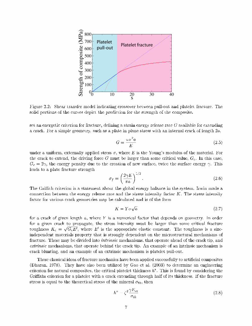
2.2 Shear transfer model indicating crossover between pull-out and platelet fracture. Thesolid portions of the curves depict the prediction for the strength of the composite. 7
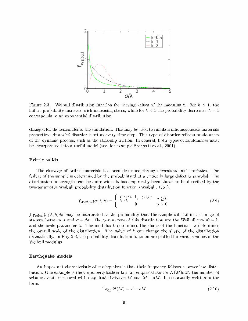
2.3 Weibull distribution function for varying values of the modulus k. For k > 1, thefailure probability increases with increasing stress, while for k < 1 the probabilitydecreases. k = 1 corresponds to an exponential distribution. . . . . . . . . . . . . . . 9
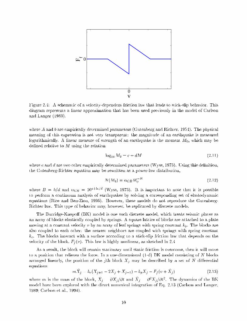
2.4 A schematic of a velocity-dependent friction law that leads to stick-slip behavior.This diagram represents a linear approximation that has been used previously in themodel of Carlson and Langer (1989). . . . . . . . . . . . . . . . . . . . . . . . . . . . 10
2.5 Schematic of a Burridge-Knopo-like spring-block model. The blocks are attachedto a plate moving at a xed velocity through leaf springs, and exhibit a stick-slipinteraction with the surface. . . . . . . . . . . . . . . . . . . . . . . . . . . . . . . . . 11
2.6 Schematic of hollow-core dislocation with initial radius R0 undergoing Rayleighbreakup. The periodicity of the perturbation is . . . . . . . . . . . . . . . . . . . . 14
2.7 Schematic of coarsening in 2-d. The initial microstructure is shown in Panel 2.7a,and the microstructure after mass transport is shown in Panel 2.7b. . . . . . . . . . 15
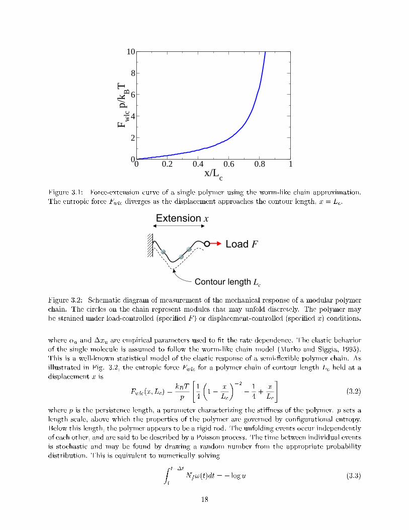
3.1 Force-extension curve of a single polymer using the worm-like chain approximation.The entropic force Fwlc diverges as the displacement approaches the contour length,x = Lc. . . . . . . . . . . . . . . . . . . . . . . . . . . . . . . . . . . . . . . . . . . . 18
3.2 Schematic diagram of measurement of the mechanical response of a modular poly-mer chain. The circles on the chain represent modules that may unfold discretely.The polymer may be strained under load-controlled (specied F ) or displacement-controlled (specied x) conditions. . . . . . . . . . . . . . . . . . . . . . . . . . . . . 18
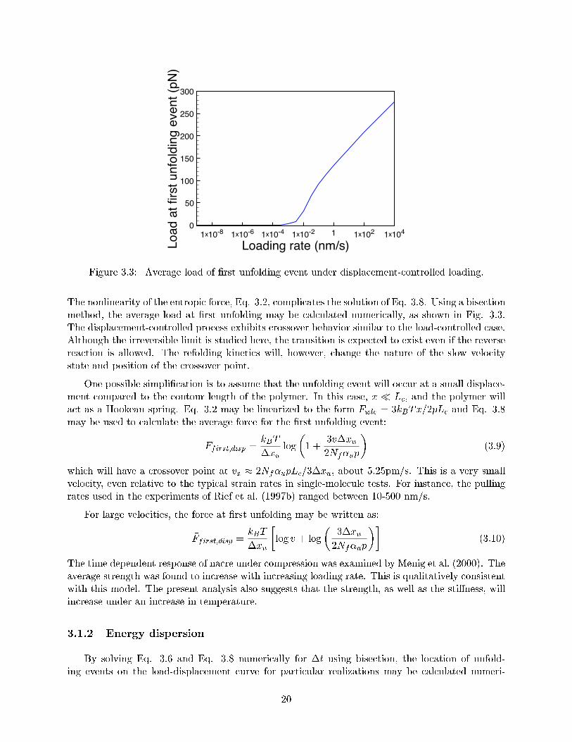
3.3 Average load of rst unfolding event under displacement-controlled loading. . . . . . 20
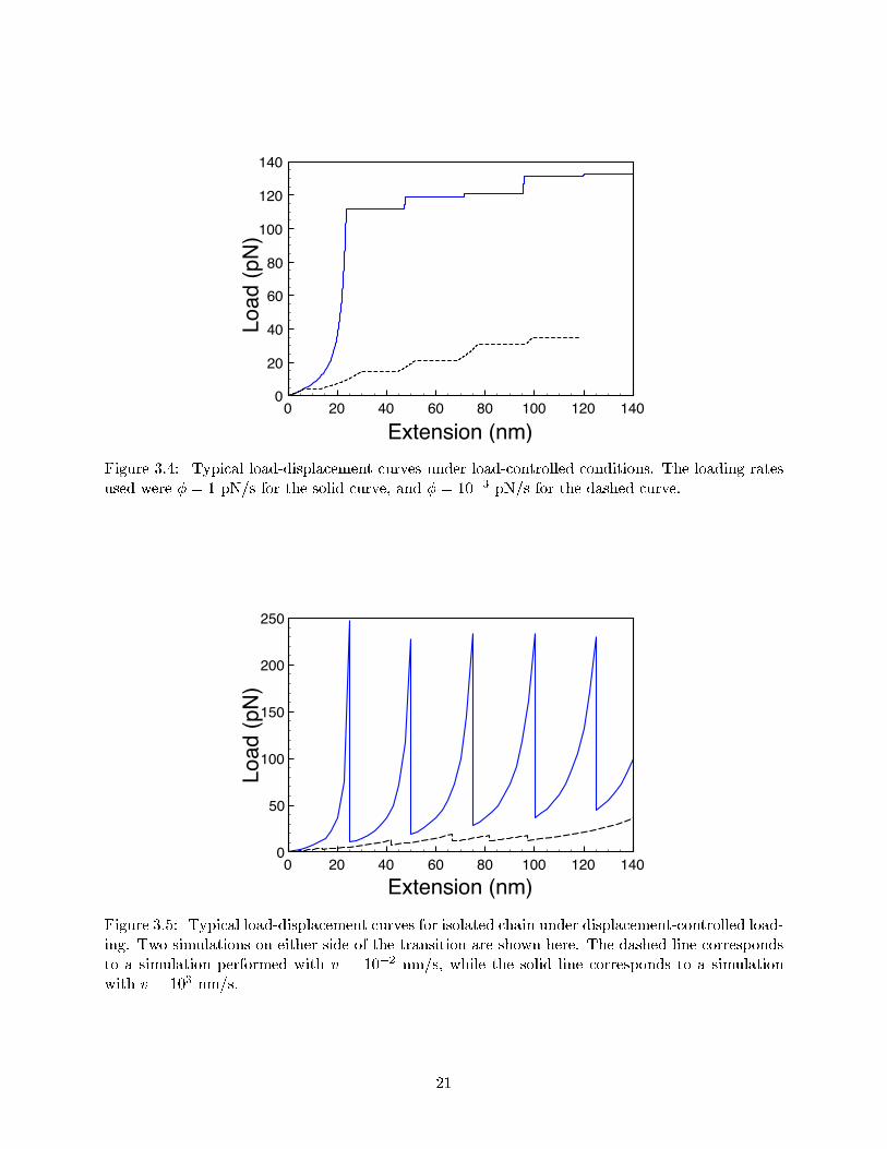
3.4 Typical load-displacement curves under load-controlled conditions. The loading ratesused were = 1 pN/s for the solid curve, and = 103 pN/s for the dashed curve. . 21
3.5 Typical load-displacement curves for isolated chain under displacement-controlledloading. Two simulations on either side of the transition are shown here. Thedashed line corresponds to a simulation performed with v = 102 nm/s, while thesolid line corresponds to a simulation with v = 103 nm/s. . . . . . . . . . . . . . . . 21
iv
3.6 Average fraction of energy dissipated during extension of polymer, W=W , underdisplacement-controlled loading. For velocities smaller than the transition velocity,vt, the energy dissipated is negligible. . . . . . . . . . . . . . . . . . . . . . . . . . . . 22
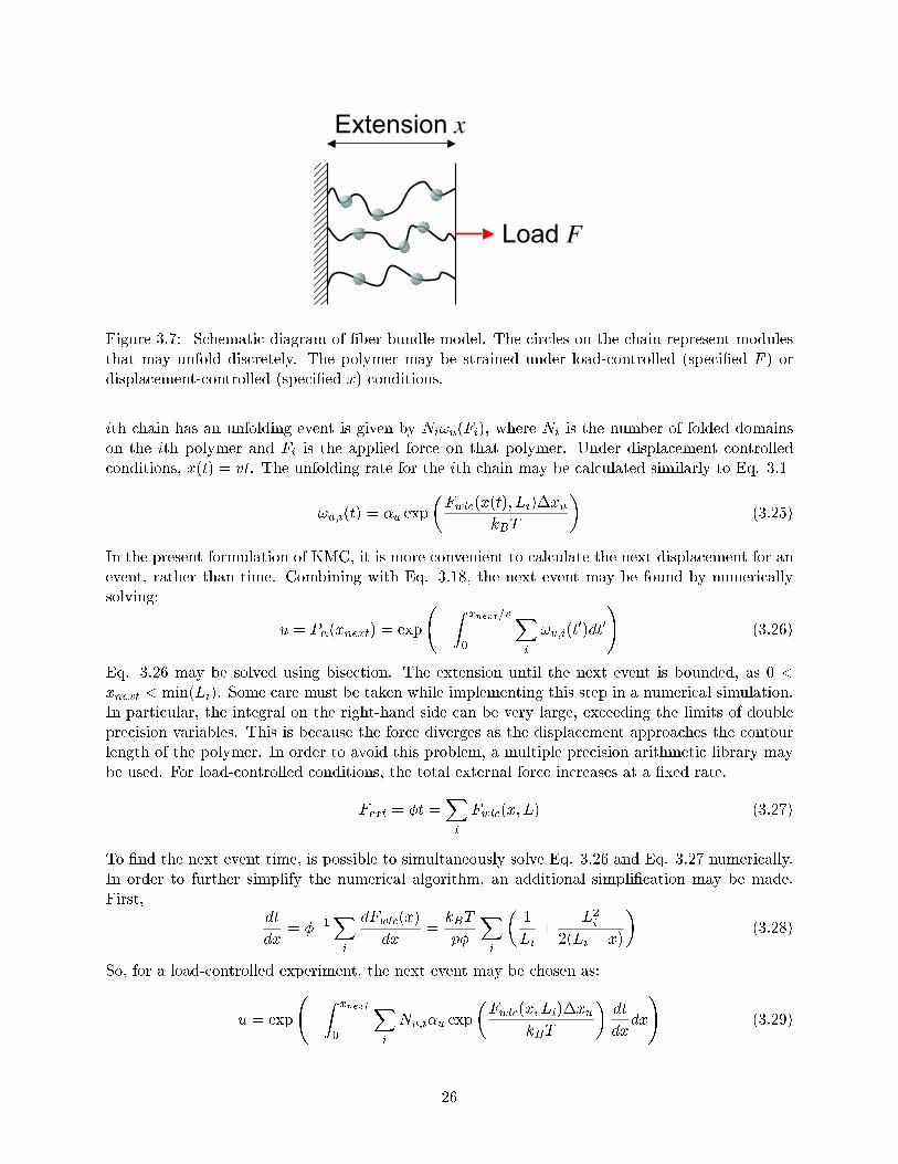
3.7 Schematic diagram of ber bundle model. The circles on the chain represent modulesthat may unfold discretely. The polymer may be strained under load-controlled(specied F ) or displacement-controlled (specied x) conditions. . . . . . . . . . . . 26
3.8 Typical results of displacement-controlled KMC simulations of FBM. Panel 3.8adepicts the load-displacement behavior for dierent values of the pulling velocity,v. The corresponding eective spring constants are shown in Panel 3.8b. In thesesimulations, N = 1000. . . . . . . . . . . . . . . . . . . . . . . . . . . . . . . . . . . . 28
3.9 Slope of the hardening region for various values of loading rate for displacement-controlled deformation (Panel 3.9a) and load-controlled deformation (Panel 3.9b).Data points are the average of 100 trials, with N = 100. The error bars are onestandard deviation. . . . . . . . . . . . . . . . . . . . . . . . . . . . . . . . . . . . . . 29
3.10 Typical results of load-controlled KMC simulations of FBM. Panel 3.10a depictsthe load-displacement behavior for dierent values of the normalized pulling rate,=N0
chains. The corresponding eective spring constants are shown in Panel 3.10b. . 31
3.11 Typical results of load-controlled bundles that are allowed to progress to failure.After the last unfolding event occurs, the polymer is removed from the simulation. . 32
3.12 Distributions of failure strengths of ber bundle models, allowing for polymer fail-ure. These failure strengths are normalized by the average failure strength for thatvelocity, hi. . . . . . . . . . . . . . . . . . . . . . . . . . . . . . . . . . . . . . . . . 32
3.13 Probability distribution of times between plastic events . . . . . . . . . . . . . . . . 33
3.14 Scaling form of plastic size events of a nonlinear ber bundle. These events are char-acterized by t, the time to the next failure event and x, the displacement associatedwith that event. The color key denotes the value of x in nm corresponding to theevent. This plot was performed using the values = 0:35 and = 0:35. . . . . . . . 34
4.1 Schematic of 2-d lattice model of nacre. The tablets are of length L and thickness t.The thickness of the organic adhesive is w. . . . . . . . . . . . . . . . . . . . . . . . . 37
4.2 Diagram of microscopic plasticity laws utilized in the lattice model. . . . . . . . . . . 39
4.3 Time evolution of damage in fuse model. A contour plot of the number of timesa particular spring has failed is plotted for a simulation applying a uniform tensilestrain in the x axis. Panel 4.3a illustrates a time sequence for damage with nomicroscopic hardening, where Panel 4.3b illustrates a time sequence with hardening.A and D represent the deformation in the elastic region, B and E represent theinitial deformation of the array and C and F depict the deformation at longer times.Qualitatively, damage is localized to a small 2-d region in the rst model, while it isspread over the entire sample in the second model. . . . . . . . . . . . . . . . . . . . 41
4.4 The damage measure Z is plotted as a function of simulation time for various levels ofthe hardening b. Larger values of the hardening spread deformation more uniformlythrough the system. . . . . . . . . . . . . . . . . . . . . . . . . . . . . . . . . . . . . 42
v
4.5 Distribution of plastic events during the deformation of a CDRFM with hardening.There is an apparent power law distribution for the CDRFM with no hardening. . . 42
4.6 Schematic of pull-out mechanism in simplied ber composite. The bers are con-nected to each other through springs with spring constant kc. They are connectedto a plate moving at a uniform velocity with springs with spring constant kp. Notethe resemblance to the BK model. . . . . . . . . . . . . . . . . . . . . . . . . . . . . 44
4.7 Dependence of depinning force on elastic constant parameters. By increasing therelative values of the spring constant, kp=kc, the force required to move the blockarray decreases. . . . . . . . . . . . . . . . . . . . . . . . . . . . . . . . . . . . . . . . 45
4.8 Atomic positions of aragonite. . . . . . . . . . . . . . . . . . . . . . . . . . . . . . . . 46
5.1 Dependence of the scaling parameter S on surface-energy anisotropy and dislocationstrength. For isotropic surface energies, the scaling factor approaches unity if R0 R. 50
5.2 Dependence of fastest-growing wavelength on critical radius for an isotropic system.This dependence depends on the active transport mechanism. The fastest-growingwavelength of systems governed by volume diusion outside of the hollow core isnotably larger than that of systems governed by volume diusion inside the hollowcore or by surface diusion. . . . . . . . . . . . . . . . . . . . . . . . . . . . . . . . . 55
5.3 Dependence of fastest-growing wavelength on surface-energy anisotropy. The domi-nant transport mechanism does not appear to strongly aect the eects of surface-energy anisotropy. . . . . . . . . . . . . . . . . . . . . . . . . . . . . . . . . . . . . . 56
5.4 Chemical potential of point defects at the surface of the dislocation core as a functionof dislocation radius. The chemical potential is normalized by =2R. There is amaximum when the particle radius is twice the Frank radius. . . . . . . . . . . . . . 57
5.5 Diagram of a simple geometry for pores coarsening on a dislocation line. Each poreis taken to be spherical with radius i and is separated from its neighbors by acenter-to-center distance d. . . . . . . . . . . . . . . . . . . . . . . . . . . . . . . . . 59
vi
List of Tables
3.1 Polymer parameters used in KMC model derived for titin (from Rief et al., 1997a). . 19
4.1 Computed structural constants of aragonite. . . . . . . . . . . . . . . . . . . . . . . . 47
4.2 Computed elastic constants of aragonite. . . . . . . . . . . . . . . . . . . . . . . . . . 47
vii
Acknowledgements
The writing of this dissertation has been supported by many friends, coworkers, and advisors.There were many times that I thought I would never nish. I am grateful to everyone who helpedme along the way- any omissions in this list are surely accidental.
I rst want to thank my advisors, Professor Daryl Chrzan and Professor Andy Glaeser, for theirsupport and guidance throughout my time here. I thank the other members of my thesis committee,Professor J. W. Morris and Professor Joel Moore for their useful suggestions and corrections to thisdocument. I thank Professor Oscar Dubon and the other members of my qualifying committee,Professor Alberto Grunbaum, Professor Didier de Fontaine and Professor R. Ramesh. I thankProfessor W. Craig Carter and Professor Samuel Allen for mentoring me at MIT. I thank ProfessorGregory Rohrer, without whom I would never have come to study ceramics. I thank his group,especially Rich Smith and Jen Giocondi.
I thank the members of the Chrzan Group: Elif Ertekin, Scott Beckman, Alex Greaney, MattSherburne, Tianshu Li, Yuranan Hanlumyuang, Shuo Chen, Karen Cheng, Priam Pillai, HillaryGreen, Kevin Long, Cosima Boswell, Diana Yi, and C. W. \Jerry" Yuan.
I thank the members of the Glaeser Group: Josh Sugar, Joe McKeown, Mary Trahanovsky,Sung Hong, Chris Bartlow, Liz Boatman, Rob Marks, and Karen Tran.
I thank my collaborators, including: Professor Robert Ritchie, Dr. Tony Tomsia, Eduardo Saiz,Daan Hein Alsem, Kurt Koester, Max Launey and Etienne Munch, Haimei Zheng, Florian Straub,Professor J. Wu, Joanne Yim, Bin Xiang, and Professor Eugene Haller.
I thank the Intel Foundation Fellowship, the National Defense Science and Engineering Grad-uate (NDSEG) Fellowship, and the Department of Energy for the funds to do the work in thisthesis.
I thank Professor Ron Gronsky and Professor Tom Devine for allowing me to teach under them.
I thank and say goodbye to Rowland Cannon, Margaret and my grandparents.
I thank my many other friends and colleagues, who have made my time in Pittsburgh, MIT,and Berkeley worthwhile: Bill, Dave, Shawn, Winterbottom, Kirsten, Yash, Katherine M, Philip,Igor, Eugene, Wenjun, Julie H., Erik, Senna, Alex Y., Trisha M., Je S., Niell, Tanya, Nicole Z.,Smitty, Lentz, Patricia M., Dan K., Anita, Leanne, Brad, Ilan, Harry, Chris L., Dr. Jay, Autumn,Navin, Laurie, Dennis, Matt P., Steph, Chris H., Ian, Jeremy M., Joanna, Padraic, Gabe, Becca J.,Becca S., Jarrett, David W., David S., Ben L., Ty, Devesh, Nicole A., Jordan, Carolyn, Cate, Rob,Scott, Joe W., Joe L., Nate, Amy, Mike S., Tommy, Q.-A., Virat, Joe W., Liz Z., Liz W., Carlton,Franklin, Doug, Craig R., Scott R., Mya, Yoshi, Patrick, Alex S., Rachel, my teammates at MIT,the MSE Ultimate Frisbee team, the Killer Wombats, the folks at the 2009 Boulder Summer School,my clubmates at BPRC, and anyone who I have forgot to mention.
I thank my family. I thank Peter, Becky, and Sara.
And of course, I thank Mom and Dad.
viii
Chapter 1
Introduction
The last thing one discovers in composing a work is what to put rst.
T. S. Eliot
A fundamental problem of materials science is understanding how and why materials fail. Themicrostructure and properties of a materials system may degrade under stress, whether the driv-ing force is mechanical, thermal, or electrical. The nature of the breakdown can determine theperformance of the material. For instance, a heterogeneous material such as concrete can developmicrocracks under an applied strain, failing gradually before a critical crack becomes unstable andpropagates. Likewise, at elevated temperature, mass diusion can become activated, causing adesirable microstructure to evolve into a less favorable one. Unfortunately, the theoretical under-standing of these processes can be dicult. Breakdown is often a non-equilibrium process thatcannot be fully described by thermodynamics. Further, the macroscopic behavior can be aectedstrongly by complex interactions between small-scale features.
One illustrative example of mechanical failure is the earthquake, where discrete bursts of energyare released due to the jerky, stick-slip motion of seismic plates. Empirical laws have been foundregarding the distributions of earthquakes. The Gutenberg-Richter law, for instance, relates thesize of an earthquake to the frequency with which it is observed. The size of an earthquake ischaracterized by its moment ad, where is the shear modulus of the rock, a is the area of thefault that slips, and d is the displacement through which this area slips. The earthquake distributionN(M0) is dened to be the number of earthquakes with moment M0 and may be written in theform:
N(M0) = GRMB0 (1.1)
where B and GR are empirically determined parameters (Wyss, 1973). Eq. 1.1 is a power-lawdistribution, which exhibits the property of scale-invariance. This is the statement that if the sizeof the earthquake is scaled by some factor , that the shape of the distribution will not change andwill instead be scaled by a factor,
N(M0) = BN(M0) (1.2)
In other words, the earthquake size distribution will show the same properties if examined ondierent size scales. N(M0) is said to have the property of generalized homogeneity: it is a scalinglaw that has no inherent size scale.
1
As stated by Barenblatt (2003), these scaling laws do not occur by accident. Their existencere ects self-similarity, a physical property of the process. To study the nature of scaling laws inearthquakes, simple models were proposed that involved dragging blocks along a surface (Burridgeand Knopo, 1967). The deformation of these models is jerky. This is because the motion ofa single block can cause avalanches. When a block slips, it changes the forces on its neighbors,and can consequently cause them to move as well. Direct numerical simulation of the equationsof motion (Carlson and Langer, 1989; Carlson et al., 1994) as well as their corresponding cellularautomaton models (Olami et al., 1992) were found to reproduce the Gutenberg-Richter law.
This example illustrates that an appropriately simplied model can exhibit the same scalingbehavior as a real system. This is understood by analogy to phase transformations. If the behaviorof these systems is in some way critical, some properties of the deformation will not depend onthe microscopic details of the interactions. For example, in earthquakes, the avalanche behaviordisappears under a suciently large force. Under certain conditions, this pinning-depinning tran-sition has been interpreted as a stress-induced phase transition (Cule and Hwa, 1996). This typeof behavior is common to a variety of dynamic systems. For instance, nonlinear conductivity insome systems has been attributed to the non-uniform sliding of charge density waves. These wavesare pinned at crystallographic defects and are prevented from moving if the applied eld is below athreshold eld (Fisher, 1985). The analogous phenomenon in magnetization has also been observed,and is known as Barkhausen noise (O'Brien and Weissman, 1994).
Dislocation plasticity on the nanoscale also progresses in discrete bursts. The force-displacementcurve from nanoindentation experiments in ductile metals exhibits a \staircase" structure (Bahret al., 1998), where each step corresponds to a plastic event. Dislocation dynamics simulationshave suggested that a pinning-depinning transition occurs in various metal systems (Chrzan andMills, 1996; Koslowski et al., 2004). Similarly, the compression of micron-sized single pillars ofNi (Dimiduk et al., 2006) and Ni superalloy (Uchic et al., 2004) have exhibited size eects thatare consistent with properties of nite size scaling. Under certain conditions, avalanche dynamicsmay cause serrations in the stress-strain curves. One example is the Portevin-Le Chatelier eect(Mazot, 1973; Balk and Lukac, 1993). In other cases, the large avalanches may be cut-o, causingthe plastic behavior to be smooth at macroscopic length scales (Zaiser and Nikitas, 2007).
Inherently stochastic phenomena, therefore, determine a physical length scale for deformation.This means that the parameters that control the engineering properties of a material may bedetermined by the statistical properties of the system. This thesis attempts to use these conceptsto understand two examples of breakdown: one mechanical and one microstructural.
The rst example of breakdown considers the eects of mechanical stresses on nacre, a naturalcomposite present in mollusk shells. Nacre consists of polycrystalline aragonite platelets connectedby an organic adhesive. It is of considerable engineering interest because its toughness is remark-ably high in comparison to the toughness of its component materials (Jackson et al., 1990). Thedominant mechanism of inelastic deformation is the sliding of these platelets. This is an inher-ently discrete process that contains a strong resemblance to the spring block model of earthquakesdescribed earlier. As a result, phenomenological models of nacre are developed to study the conse-quences of discrete deformation events.
The second example of breakdown focuses on the eect of diusion on a model microstructure,the hollow-core dislocation. Under certain conditions, this structure is unstable to shape changes.For instance, this structure may evolve to form an array of pores. The nature of the break-up
2

aects the geometry of this pore array. In particular, the mass transport mechanism determinesthe rate at which a particular perturbation grows, and so aects the nal spacing of the pore array.
3
Chapter 2
Background
Existence is a series of footnotes to a vast, obscure, unnished masterpiece.
Vladimir Nabokov
2.1 Mechanical instabilities in biological composites
2.1.1 Mechanical properties of nacre
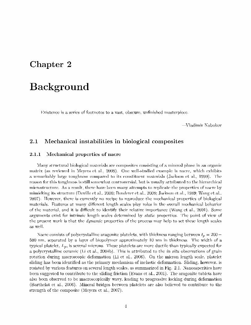
Many structural biological materials are composites consisting of a mineral phase in an organicmatrix (as reviewed in Meyers et al., 2008). One well-studied example is nacre, which exhibitsa remarkably large toughness compared to its constituent materials (Jackson et al., 1990). Thereason for this toughness is still somewhat controversial, but is usually attributed to the hierarchicalmicrostructure. As a result, there have been many attempts to replicate the properties of nacre bymimicking its structure (Deville et al., 2006; Bonderer et al., 2008; Jackson et al., 1989; Wang et al.,2007). However, there is currently no recipe to reproduce the mechanical properties of biologicalmaterials. Features at many dierent length scales play roles in the overall mechanical behaviorof the material, and it is dicult to identify their relative importance (Wang et al., 2001). Somearguments exist for intrinsic length scales determined by static properties. The point of view ofthe present work is that the dynamic properties of the process may help to set these length scalesas well.
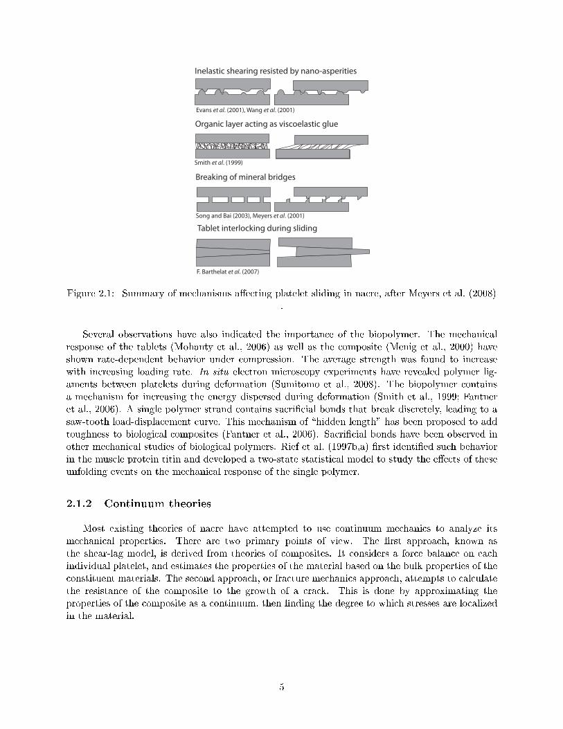
Nacre consists of polycrystalline aragonite platelets, with thickness ranging between tp = 200500 nm, separated by a layer of biopolymer approximately 10 nm in thickness. The width of atypical platelet, Lp, is several microns. These platelets are more ductile than typically expected fora polycrystalline ceramic (Li et al., 2004b). This is attributed to the in situ observations of grainrotation during macroscopic deformation (Li et al., 2006). On the micron length scale, plateletsliding has been identied as the primary mechanism of inelastic deformation. Sliding, however, isresisted by various features on several length scales, as summarized in Fig. 2.1. Nanoasperities havebeen suggested to contribute to the sliding friction (Evans et al., 2001). The aragonite tablets havealso been observed to be macroscopically wavy, leading to progressive locking during deformation(Barthelat et al., 2006). Mineral bridges between platelets are also believed to contribute to thestrength of the composite (Meyers et al., 2007).
4
Evans et al. (2001), Wang et al. (2001)
Smith et al. (1999)
Song and Bai (2003), Meyers et al. (2001)
Inelastic shearing resisted by nano-asperities
Organic layer acting as viscoelastic glue
Breaking of mineral bridges
Tablet interlocking during sliding
F. Barthelat et al. (2007)
Figure 2.1: Summary of mechanisms aecting platelet sliding in nacre, after Meyers et al. (2008).
Several observations have also indicated the importance of the biopolymer. The mechanicalresponse of the tablets (Mohanty et al., 2006) as well as the composite (Menig et al., 2000) haveshown rate-dependent behavior under compression. The average strength was found to increasewith increasing loading rate. In situ electron microscopy experiments have revealed polymer lig-aments between platelets during deformation (Sumitomo et al., 2008). The biopolymer containsa mechanism for increasing the energy dispersed during deformation (Smith et al., 1999; Fantneret al., 2006). A single polymer strand contains sacricial bonds that break discretely, leading to asaw-tooth load-displacement curve. This mechanism of \hidden length" has been proposed to addtoughness to biological composites (Fantner et al., 2006). Sacricial bonds have been observed inother mechanical studies of biological polymers. Rief et al. (1997b,a) rst identied such behaviorin the muscle protein titin and developed a two-state statistical model to study the eects of theseunfolding events on the mechanical response of the single polymer.
2.1.2 Continuum theories
Most existing theories of nacre have attempted to use continuum mechanics to analyze itsmechanical properties. There are two primary points of view. The rst approach, known asthe shear-lag model, is derived from theories of composites. It considers a force balance on eachindividual platelet, and estimates the properties of the material based on the bulk properties of theconstituent materials. The second approach, or fracture mechanics approach, attempts to calculatethe resistance of the composite to the growth of a crack. This is done by approximating theproperties of the composite as a continuum, then nding the degree to which stresses are localizedin the material.
5
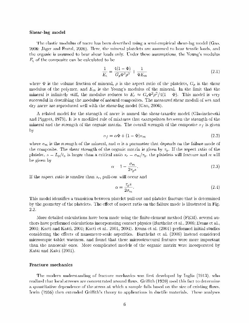
Shear-lag model
The elastic modulus of nacre has been described using a semi-empirical shear-lag model (Gao,2006; Jager and Fratzl, 2000). Here, the mineral platelets are assumed to bear tensile loads, andthe organic is assumed to bear shear loads only. Under these assumptions, the Young's modulusEc of the composite can be calculated to be
1
Ec=
4(1 )
Gp22+
1
Em(2.1)
where is the volume fraction of mineral, is the aspect ratio of the platelets, Gp is the shearmodulus of the polymer, and Em is the Young's modulus of the mineral. In the limit that themineral is innitely sti, the modulus reduces to Ec Gp
22=4(1 ). This model is verysuccessful in describing the modulus of natural composites. The measured shear moduli of wet anddry nacre are reproduced well with the shear-lag model (Gao, 2006).
A related model for the strength of nacre is named the shear-transfer model (Glavinchevskiand Piggott, 1973). It is a modied rule of mixtures that extrapolates between the strength of themineral and the strength of the organic matrix. The overall strength of the composite f is givenby
f = + (1 )m (2.2)
where m is the strength of the mineral, and is a parameter that depends on the failure mode ofthe composite. The shear strength of the organic matrix is given by y. If the aspect ratio of theplatelet, s = Lp=tp is larger than a critical ratio sc = m=y, the platelets will fracture and willbe given by
= 1 m2ys
: (2.3)
If the aspect ratio is smaller than sc, pull-out will occur and
=ys
2m: (2.4)
This model identies a transition between platelet pull-out and platelet fracture that is determinedby the geometry of the platelets. The eect of aspect ratio on the failure mode is illustrated in Fig.2.2.
More detailed calculations have been made using the nite-element method (FEM). several au-thors have performed calculations incorporating contact physics (Barthelat et al., 2006; Evans et al.,2001; Katti and Katti, 2001; Katti et al., 2001, 2004). Evans et al. (2001) performed initial studiesconsidering the eects of nanometer-scale asperities. Barthelat et al. (2006) instead consideredmicroscopic tablet waviness, and found that these microstructural features were more importantthan the nanoscale ones. More complicated models of the organic matrix were incorporated byKatti and Katti (2001).
Fracture mechanics
The modern understanding of fracture mechanics was rst developed by Inglis (1913), whorealized that local stresses are concentrated around aws. Grith (1920) used this fact to determinea quantitative dependence of the stress at which a sample fails based on the size of existing aws.Irwin (1956) then extended Grith's theory to applications in ductile materials. These analyses
6
0 10 20 30 40s0
100200300400500600700800
Stre
ngth
of c
ompo
site
(MPa
)
Platelet fracturePlateletpull-out
Figure 2.2: Shear transfer model indicating crossover between pull-out and platelet fracture. Thesolid portions of the curves depict the prediction for the strength of the composite.
set an energetic criterion for fracture, dening a strain energy release rate G available for extendinga crack. For a simple geometry, such as a plate in plane stress with an internal crack of length 2a,
G =2a
E(2.5)
under a uniform, externally applied stress , where E is the Young's modulus of the material. Forthe crack to extend, the driving force G must be larger than some critical value, Gc. In this case,Gc = 2 , the energy penalty due to the creation of new surface, twice the surface energy . Thisleads to a plate fracture strength
f =
2 E
a
1=2
: (2.6)
The Grith criterion is a statement about the global energy balance in the system. Irwin made aconnection between the energy release rate and the stress intensity factor K. The stress intensityfactor for various crack geometries may be calculated and is of the form
K = Y pa (2.7)
for a crack of given length a, where Y is a numerical factor that depends on geometry. In orderfor a given crack to propagate, the stress intensity must be larger than some critical fracturetoughness Kc =
pGcE0, where E0 is the appropriate elastic constant. The toughness is a size-
independent materials property that is strongly dependent on the microstructural mechanisms offracture. These may be divided into intrinsic mechanisms, that operate ahead of the crack tip, andextrinsic mechanisms, that operate behind the crack tip. An example of an intrinsic mechanism iscrack blunting, and an example of an extrinsic mechanism is platelet pull-out.
These classical ideas of fracture mechanics have been applied successfully to articial composites(Dharan, 1978). They have also been utilized by Gao et al. (2003) to determine an engineeringcriterion for natural composites, the critical platelet thickness h. This is found by considering theGriths criterion for a platelet with a crack extending through half of its thickness. If the fracturestress is equal to the theoretical stress of the mineral th, then
h = 2 Em
th(2.8)
7

where is a numerical factor of order one, and Em is the Young's modulus of the mineral. isthe surface energy of the mineral. Gao et al. (2003) argues that the strength of platelets largerthan this length will be determined by internal aws. So, h denes an inherent length scale of theplatelets. Assuming = 1 J/m2, = 1, Em = 100 GPa, and = Em=30, h
is estimated to beabout 30 nm. One of the attractive aspects of this theory is that all of the parameters in Eq. 2.8may be calculated through direct atomistic scale simulations.
Other researchers have attempted to consider alternate theories of elasticity. One such theoryis the Cosserat, or micropolar theory of elasticity (Eringen, 1966). This theory incorporates localrotations into its formalism. This leads to elastic deformation of materials exhibiting an inherentlength scale. Using elasticity theory, the stress concentration factor depends only on the shape ofthe hole or inclusion. However, under Cosserat theory, the stress concentration factor also is foundto depend on the size of the inhomogeneity. This theory has been used to address how microscopicfeatures in bone such as osteons introduce a size scale into the elastic response of the material(Lakes, 1995).
2.1.3 Statistical mechanics approach
Fracture in metals has been understood as a phase transformation (Hilarov, 2005). This suggestsanother way to understand the size dependence of the strength of solids. This point of view was alsosuggested by Mandelbrot et al. (1984), who found that fracture surfaces in metals have a fractalshape, and further claimed the fractal dimension of the surface is correlated to the toughness ofthe material. In other words, there is a possible connection between the engineering property oftoughness and the self-similar characteristics of the fracture process. This suggests the utility ofapplying techniques of statistical mechanics to the problem of fracture.
A few studies have specically considered the consequences of the randommicroscopic propertieson the engineering properties of nacre. Nukala and Simunovic (2005) proposed a statistical modelfor nacre using an electrical analogue of fuses and resistors. By modeling the material as a set ofelements that fail completely at a threshold extension, a design criterion for the maximum load oneach platelet can be predicted. Because the material properties are inhomogeneous, it is not trivialto calculate this quantity from the shear-lag model.
Another indication of the importance of distributions of material properties on the structuralproperties of nacre comes from the continuum elastic calculations of Barthelat et al. (2006). Thestrength of an array of perfect, hexagonal platelets was found to be lower than that of a morerealistic microstructure. This result suggests that the randomness in the structure is connected tothe mechanical response of the system.
A third important observation is that a power-law relationship exists between the size andfrequency of acoustic emission events in bone and deer antler (Zioupos et al., 1994) during fracture.This suggests that plastic events in natural composites are discrete, analogous to earthquakes.
Because of these issues, it is dicult to study statistical eects using the traditional methodsof continuum mechanics. As a result, simplied models were developed to study fracture in othersystems (as reviewed in Herrmann and Roux, 1990; Krajcinovic and Mier, 2000). In particular,fracture has been studied in the context of earthquakes, textiles, and dielectric breakdown. Someimportant results of these theories are described in this section. There are a large variety oftechniques that have been developed: this is partly because disorder may be incorporated in twodierent ways. Quenched disorder refers to properties that are initially set randomly then not
8
0 1 2 3 4 5σ/λ
0
1
2
f Wei
bull
k=0.5k=1k=2
Figure 2.3: Weibull distribution function for varying values of the modulus k. For k > 1, thefailure probability increases with increasing stress, while for k < 1 the probability decreases. k = 1corresponds to an exponential distribution.
changed for the remainder of the simulation. This may be used to simulate inhomogeneous materialsproperties. Annealed disorder is set at every time step. This type of disorder re ects randomnessof the dynamic process, such as the stick-slip friction. In general, both types of randomness mustbe incorporated into a useful model (see, for example Scorretti et al., 2001).
Brittle solids
The cleavage of brittle materials has been described through \weakest-link" statistics. Thefailure of the sample is determined by the probability that a critically large defect is sampled. Thedistribution in strengths can be quite wide: it has empirically been shown to be described by thetwo-parameter Weibull probability distribution function (Weibull, 1951).
fWeibull(;; k) =
(k
k1e(=)
k 0
0 0(2.9)
fWeibull(;; k)d may be interpreted as the probability that the sample will fail in the range ofstresses between and + d. The parameters of this distribution are the Weibull modulus k,and the scale parameter . The modulus k determines the shape of the function. determinesthe overall scale of the distribution. The value of k can change the shape of the distributiondramatically. In Fig. 2.3, the probability distribution function are plotted for various values of theWeibull modulus.
Earthquake models
An important characteristic of earthquakes is that their frequency follows a power-law distri-bution. One example is the Gutenberg-Richter law, an empirical law for N(M)dM , the number ofseismic events measured with magnitude between M and M + dM . It is normally written in theform:
log10N(M) = A bM (2.10)
9
0v
0F f
Figure 2.4: A schematic of a velocity-dependent friction law that leads to stick-slip behavior. Thisdiagram represents a linear approximation that has been used previously in the model of Carlsonand Langer (1989).
where A and b are empirically determined parameters (Gutenberg and Richter, 1954). The physicalmeaning of this expression is not very transparent: the magnitude of an earthquake is measuredlogarithmically. A linear measure of strength of an earthquake is the moment M0, which may bedened relative to M using the relation
log10M0 = c+ dM (2.11)
where c and d are two other empirically determined parameters (Wyss, 1973). Using this denition,the Gutenberg-Richter equation may be rewritten as a power-law distribution,
N(M0) = GRMB0 (2.12)
where B = b=d and GR = 10a+bc=d (Wyss, 1973). It is important to note that it is possibleto perform a continuum analysis of earthquakes by solving a corresponding set of elastodynamicequations (Rice and Ben-Zion, 1996). However, these models do not reproduce the Gutenberg-Richter law. This type of behavior may, however, be replicated by discrete models.
The Burridge-Knopo (BK) model is one such discrete model, which treats seismic plates asan array of blocks elastically coupled by springs. A square lattice of blocks are attached to a platemoving at a constant velocity v by an array of leaf springs with spring constant kp. The blocks arealso coupled to each other: the nearest neighbors are coupled with springs with spring constantkc. The blocks interact with a surface according to a stick-slip friction law that depends on thevelocity of the block, Ff (v). This law is highly nonlinear, as sketched in 2.4
As a result, the block will remain stationary until static friction is overcome, then it will moveto a position that relieves the force. In a one-dimensional (1-d) BK model consisting of N blocksarranged linearly, the position of the jth block Xj may be described by a set of N dierentialequations
m Xj = kc(Xj+1 2Xj +Xj1) kpXj Ff (v + _Xj) (2.13)
where m is the mass of the block, _Xj = @Xj=@t and Xj = @2Xj=@t2. The dynamics of the BK
model have been explored with the direct numerical integration of Eq. 2.13 (Carlson and Langer,1989; Carlson et al., 1994).
10
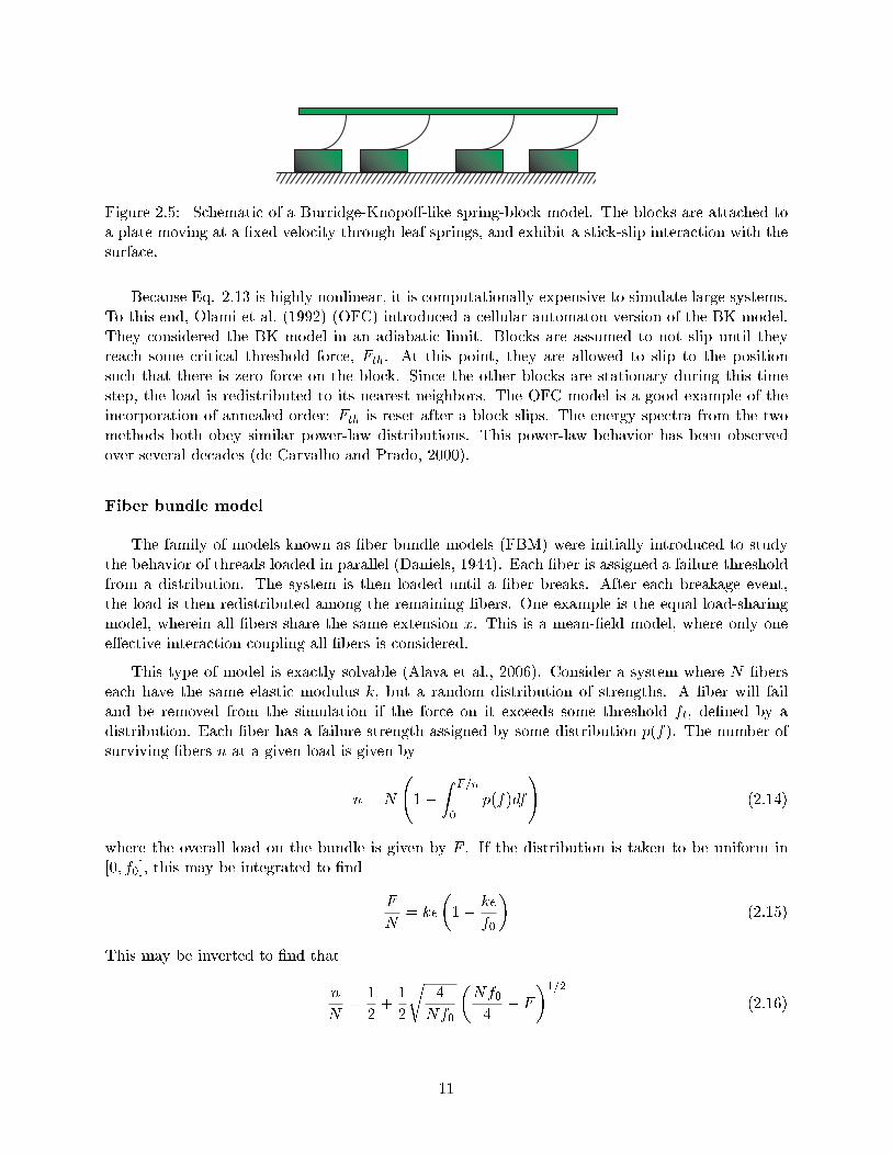
Figure 2.5: Schematic of a Burridge-Knopo-like spring-block model. The blocks are attached toa plate moving at a xed velocity through leaf springs, and exhibit a stick-slip interaction with thesurface.
Because Eq. 2.13 is highly nonlinear, it is computationally expensive to simulate large systems.To this end, Olami et al. (1992) (OFC) introduced a cellular automaton version of the BK model.They considered the BK model in an adiabatic limit. Blocks are assumed to not slip until theyreach some critical threshold force, Fth. At this point, they are allowed to slip to the positionsuch that there is zero force on the block. Since the other blocks are stationary during this timestep, the load is redistributed to its nearest neighbors. The OFC model is a good example of theincorporation of annealed order: Fth is reset after a block slips. The energy spectra from the twomethods both obey similar power-law distributions. This power-law behavior has been observedover several decades (de Carvalho and Prado, 2000).
Fiber bundle model
The family of models known as ber bundle models (FBM) were initially introduced to studythe behavior of threads loaded in parallel (Daniels, 1944). Each ber is assigned a failure thresholdfrom a distribution. The system is then loaded until a ber breaks. After each breakage event,the load is then redistributed among the remaining bers. One example is the equal load-sharingmodel, wherein all bers share the same extension x. This is a mean-eld model, where only oneeective interaction coupling all bers is considered.
This type of model is exactly solvable (Alava et al., 2006). Consider a system where N berseach have the same elastic modulus k, but a random distribution of strengths. A ber will failand be removed from the simulation if the force on it exceeds some threshold ft, dened by adistribution. Each ber has a failure strength assigned by some distribution p(f). The number ofsurviving bers n at a given load is given by
n = N
1
Z F=n
0p(f)df
!(2.14)
where the overall load on the bundle is given by F . If the distribution is taken to be uniform in[0; f0], this may be integrated to nd
F
N= k
1 k
f0
(2.15)
This may be inverted to nd that
n
N=
1
2+1
2
r4
Nf0
Nf04
F
1=2
(2.16)
11
This form suggests that there is a critical load on a ber bundle Fc = Nf0=4, above which thedeformation causes catastrophic failure. It is interesting to note that
@n
@F=
sN
4f0(Fc F )1=2 (2.17)
This analysis demonstrates that the rate of bond fractures increases very rapidly as the systemapproaches catastrophic failure.
Because of the simplicity of the FBM, a variety of modications have been proposed and studied.In order to incorporate spatial eects, local load-sharing models have also been proposed. In suchmodels, instead of the load being distributed equally among the survivors, the load is shed to thenearest neighbors. Changing to a local load-sharing condition changes the size dependence of theproperties. In particular, the average bundle strength scales as 1= log(N) (Kloster et al., 1997).
Allowing local redistributions of strain allows the organization of the bers within the bundleto aect the mechanical behavior of the bundle. To this end, hierarchical distributions of berbundles have been studied computationally (Newman and Gabrielov, 1991). FBM have also beenused to study dynamic fracture. Marder (1993) considered a 1-d dynamic version of a local-loadsharing FBM that included inertial masses at each node.
Random-fuse model
A statistical method that allows the study of spatial correlations between failure events is therandom-fuse model (RFM). An electrical network of resistors is connected through fuses (de Ar-cangelis et al., 1985). The threshold of each fuse is taken from a statistical distribution. This wasintroduced as an analogue to mechanical fracture. Unlike the equal-load sharing FBM discussedearlier, the RFM is inherently non-local.
Random properties may be incorporated into this model in multiple ways. For instance, thediluted model contains fuses with uniform failure thresholds. The term dilution refers to prebreakinga certain number of bonds. These models are brittle. Alternatively, the failure strengths of thefuses may be taken to be random. In this case, the inhomogeneous fuse strengths can cause crackde ection and a more gradual failure (Kahng et al., 1988; Sahimi and Goddard, 1986). This limit isknown as strong disorder. Other models have explicitly incorporated other toughening mechanisms.For instance, ber bridging in ber-reinforced composites may be modeled by introducing a remnantresistivity that remains after the initial fuse fails (Li and Duxbury, 1988).
Using an RFM where the strengths of the fuses are drawn from a random distribution, somescaling behavior was identied. (de Arcangelis et al., 1989). The RFM may be thought of asa discrete elastic model. It may be similarly modied extensively because of its simplicity. Forinstance, the fuses of the RFM may be replaced with elastic beams in the bond-bending model.It may be shown that in the continuum limit the beam and bond-bending models reduce to themicropolar theory of elasticity (Herrmann and Roux, 1990).
Another important generalization of the RFM is the inclusion of plasticity. One example is thecontinuous-damage random-fuse model (CDRFM), as introduced by Zapperi et al. (1997). Thismodel was formulated in order to simulate plastic deformation: it allows each spring to fail multipletimes.
12
2.1.4 Summary
Nacre is a natural composite with an inherently discrete, hierarchical structure. A numberof models have been developed in order to study the mechanical deformation of various materialswith discrete elements. They exhibit complex stick-slip dynamics. The consequences of this jerkydeformation process on the mechanical properties of nacre have not yet been fully understood. Bydoing so, it may be possible to determine engineering criteria that may be used to explain thetoughness of nacre.
2.2 Capillary instabilities in strained systems
Under elevated temperatures, mass-transport mechanisms such as diusion become active. Mosttechnically important microstructures are not thermodynamically stable with respect to surfaceenergy, and will therefore evolve to minimize the surface energy of the system. This is known asa capillary instability. In solid materials, there is often a competition between surface energy andstrain energy. For instance, Cahn (1957) proposed that strain energy can modify the kinetics ofheterogeneous nucleation. If a precipitate forms on a dislocation, strain energy is relieved at theexpense of generating new interfaces. This idea has recently been exploited as a route to fabricatenanometer-scale wires (Nakamura et al., 2003).
In order to study these phenomena theoretically, it is necessary to make simplifying assumptions.In particular, the dynamics are assumed to be self-similar. This approach was initially used inthe context of powder processing by Herring (1950). Under this assumption, the morphologicalevolution of a system undergoing sintering may be described by a scaling law. The exponent ofthis scaling law is determined by identity of the dominant mass transport process.
2.2.1 Hollow-core dislocations
A technologically important microstructural feature is the hollow-core dislocation, or\nanopipe." Interest in these defects has recently been revived due to their detrimental pres-ence in electronic materials. For instance, Neudeck and Powell (1994) claimed that the presenceof nanopipes can be the limiting factor in the performance of SiC power devices. Hollow-coredislocations have been observed in SiC at growth spirals (Verma, 1953). Further, hollow-coredislocations have been observed as defects in AlN thin lms (Tokumoto et al., 2008) and GaN thinlms (Qian et al., 1995).
Frank (1951) rst proposed that material near the dislocation core may be transported awayand the core may open, decreasing the elastic-strain energy at the expense of creating free surfaces.In particular, a thermodynamically stable radius is predicted that depends on the size of theBurgers vector of the dislocation, the elastic moduli, and the surface energy. However, the theoryof Frank (1951) does not quantitatively predict the sizes of experimentally observed hollow-coredislocations. As a result, more detailed theories have been proposed. In particular, the stabilityof these defects has been considered when the crystal is growing or evaporating (Cabrera andLevine, 1956). This model was improved to better treat the non-linear behavior near the core by(Schaarachter, 1965a,b). van der Hoek et al. (1982) introduced a strain energy function for thedislocation core that sets a dierent thermodynamic condition for nanopipe stability.
More detailed formation mechanisms for the hollow-core dislocation have been proposed, incor-
13
z
λ
2R0
2Rmat
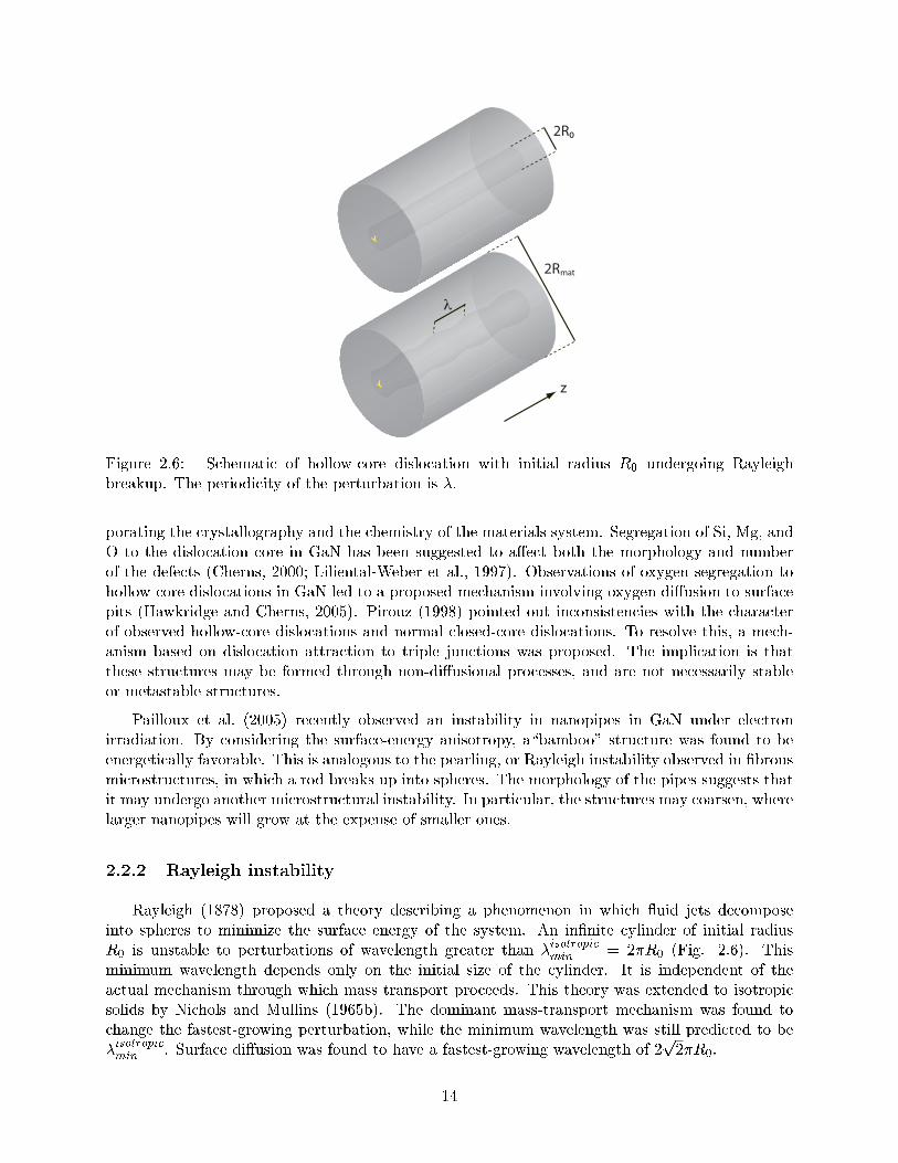
Figure 2.6: Schematic of hollow-core dislocation with initial radius R0 undergoing Rayleighbreakup. The periodicity of the perturbation is .
porating the crystallography and the chemistry of the materials system. Segregation of Si, Mg, andO to the dislocation core in GaN has been suggested to aect both the morphology and numberof the defects (Cherns, 2000; Liliental-Weber et al., 1997). Observations of oxygen segregation tohollow-core dislocations in GaN led to a proposed mechanism involving oxygen diusion to surfacepits (Hawkridge and Cherns, 2005). Pirouz (1998) pointed out inconsistencies with the characterof observed hollow-core dislocations and normal closed-core dislocations. To resolve this, a mech-anism based on dislocation attraction to triple junctions was proposed. The implication is thatthese structures may be formed through non-diusional processes, and are not necessarily stableor metastable structures.
Pailloux et al. (2005) recently observed an instability in nanopipes in GaN under electronirradiation. By considering the surface-energy anisotropy, a\bamboo" structure was found to beenergetically favorable. This is analogous to the pearling, or Rayleigh instability observed in brousmicrostructures, in which a rod breaks up into spheres. The morphology of the pipes suggests thatit may undergo another microstructural instability. In particular, the structures may coarsen, wherelarger nanopipes will grow at the expense of smaller ones.
2.2.2 Rayleigh instability
Rayleigh (1878) proposed a theory describing a phenomenon in which uid jets decomposeinto spheres to minimize the surface energy of the system. An innite cylinder of initial radiusR0 is unstable to perturbations of wavelength greater than isotropicmin = 2R0 (Fig. 2.6). Thisminimum wavelength depends only on the initial size of the cylinder. It is independent of theactual mechanism through which mass transport proceeds. This theory was extended to isotropicsolids by Nichols and Mullins (1965b). The dominant mass-transport mechanism was found tochange the fastest-growing perturbation, while the minimum wavelength was still predicted to beisotropicmin . Surface diusion was found to have a fastest-growing wavelength of 2
p2R0.
14
(a) (b)
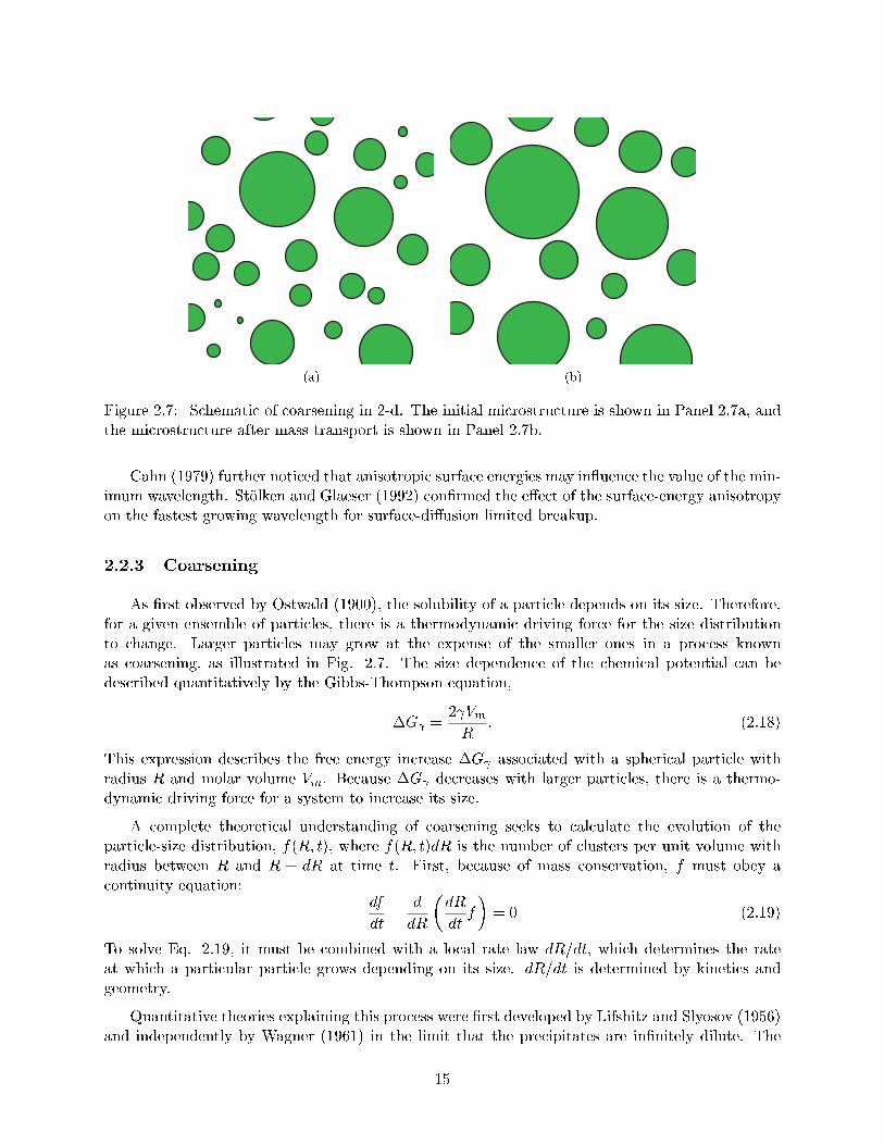
Figure 2.7: Schematic of coarsening in 2-d. The initial microstructure is shown in Panel 2.7a, andthe microstructure after mass transport is shown in Panel 2.7b.
Cahn (1979) further noticed that anisotropic surface energies may in uence the value of the min-imum wavelength. Stolken and Glaeser (1992) conrmed the eect of the surface-energy anisotropyon the fastest growing wavelength for surface-diusion limited breakup.
2.2.3 Coarsening
As rst observed by Ostwald (1900), the solubility of a particle depends on its size. Therefore,for a given ensemble of particles, there is a thermodynamic driving force for the size distributionto change. Larger particles may grow at the expense of the smaller ones in a process knownas coarsening, as illustrated in Fig. 2.7. The size dependence of the chemical potential can bedescribed quantitatively by the Gibbs-Thompson equation,
G =2 VmR
: (2.18)
This expression describes the free energy increase G associated with a spherical particle withradius R and molar volume Vm. Because G decreases with larger particles, there is a thermo-dynamic driving force for a system to increase its size.
A complete theoretical understanding of coarsening seeks to calculate the evolution of theparticle-size distribution, f(R; t), where f(R; t)dR is the number of clusters per unit volume withradius between R and R + dR at time t. First, because of mass conservation, f must obey acontinuity equation:
df
dt+
d
dR
dR
dtf
= 0 (2.19)
To solve Eq. 2.19, it must be combined with a local rate law dR=dt, which determines the rateat which a particular particle grows depending on its size. dR=dt is determined by kinetics andgeometry.
Quantitative theories explaining this process were rst developed by Lifshitz and Slyosov (1956)and independently by Wagner (1961) in the limit that the precipitates are innitely dilute. The
15
diusion equation is solved for an isolated particle. This leads to a simple form for the rate law.For instance, dR=dt for spheres undergoing diusion-limited growth may be written as:
dR
dt=K
diff
R2
R
Rc 1
(2.20)
where Kdiff is a rate constant, and Rc is the critical radius. This so-called LSW theory predicts
the average particle radius increases with time according to a power law hR(t)ni / t, where thevalue of n depends on the dominant growth mechanism. For the coarsening of spheres under adiusion-limited growth law, n = 3.
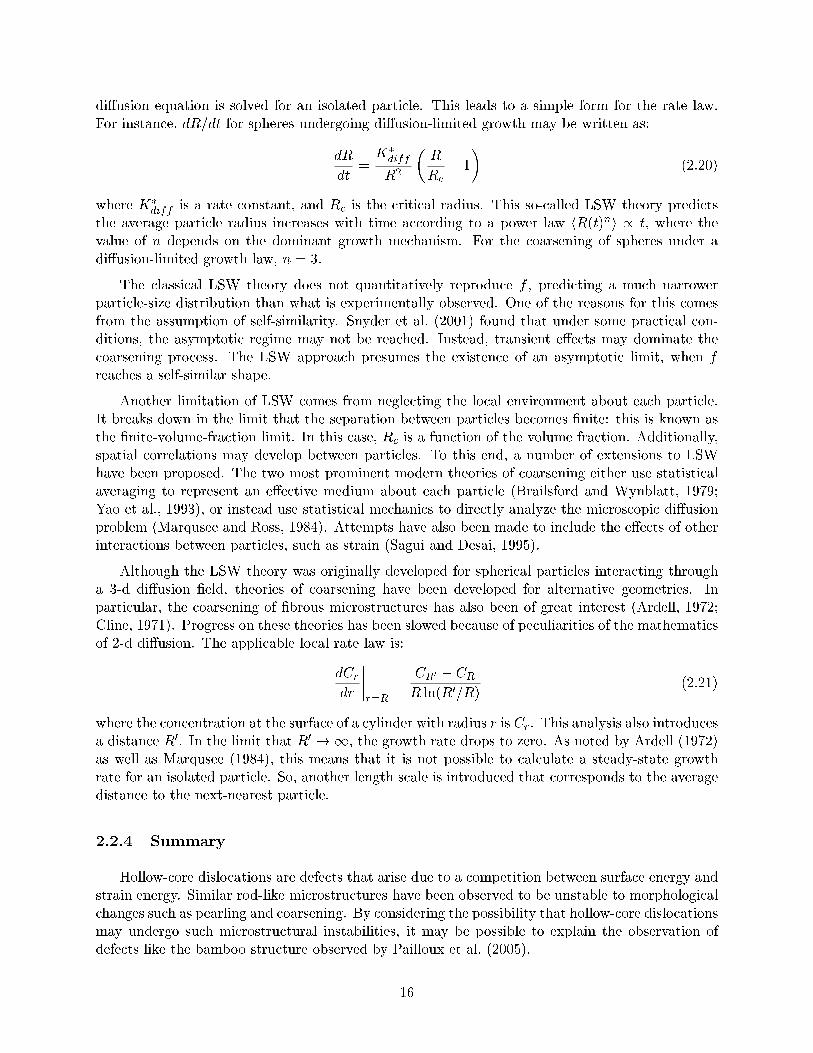
The classical LSW theory does not quantitatively reproduce f , predicting a much narrowerparticle-size distribution than what is experimentally observed. One of the reasons for this comesfrom the assumption of self-similarity. Snyder et al. (2001) found that under some practical con-ditions, the asymptotic regime may not be reached. Instead, transient eects may dominate thecoarsening process. The LSW approach presumes the existence of an asymptotic limit, when freaches a self-similar shape.
Another limitation of LSW comes from neglecting the local environment about each particle.It breaks down in the limit that the separation between particles becomes nite: this is known asthe nite-volume-fraction limit. In this case, Rc is a function of the volume fraction. Additionally,spatial correlations may develop between particles. To this end, a number of extensions to LSWhave been proposed. The two most prominent modern theories of coarsening either use statisticalaveraging to represent an eective medium about each particle (Brailsford and Wynblatt, 1979;Yao et al., 1993), or instead use statistical mechanics to directly analyze the microscopic diusionproblem (Marqusee and Ross, 1984). Attempts have also been made to include the eects of otherinteractions between particles, such as strain (Sagui and Desai, 1995).
Although the LSW theory was originally developed for spherical particles interacting througha 3-d diusion eld, theories of coarsening have been developed for alternative geometries. Inparticular, the coarsening of brous microstructures has also been of great interest (Ardell, 1972;Cline, 1971). Progress on these theories has been slowed because of peculiarities of the mathematicsof 2-d diusion. The applicable local rate law is:
dCr
dr
r=R
=CR0 CR
R ln(R0=R)(2.21)
where the concentration at the surface of a cylinder with radius r is Cr. This analysis also introducesa distance R0. In the limit that R0 !1, the growth rate drops to zero. As noted by Ardell (1972)as well as Marqusee (1984), this means that it is not possible to calculate a steady-state growthrate for an isolated particle. So, another length scale is introduced that corresponds to the averagedistance to the next-nearest particle.
2.2.4 Summary
Hollow-core dislocations are defects that arise due to a competition between surface energy andstrain energy. Similar rod-like microstructures have been observed to be unstable to morphologicalchanges such as pearling and coarsening. By considering the possibility that hollow-core dislocationsmay undergo such microstructural instabilities, it may be possible to explain the observation ofdefects like the bamboo structure observed by Pailloux et al. (2005).
16
Chapter 3
Dynamic model of plastic deformation
in nacre
The rst man gets the oyster, the second man gets the shell.
Andrew Carnegie
One mechanism that has been proposed as the reason for the high toughness for nacre is thatenergy may be dispersed during the inelastic deformation of the biopolymer. In particular, discretedomains on the matrix biopolymer Lustrin A may unfold, eectively increasing the length of thechain (Smith et al., 1999). There is inelastic deformation associated with sacricial bonds thatcauses the dissipation of energy during deformation. A closely related mechanism has been used tounderstand the deformation of biopolymers in bone. The side groups in proteins such as osteopontinand dental matrix protein 1 have similarly been proposed to interact, leading to another type ofsacricial bond that may aect the mechanical behavior of bone (Fantner et al., 2007; Adams et al.,2008).
3.1 Dynamic response of a single biopolymer
The breaking of sacricial bonds in a biopolymer is an inherently stochastic process. It may beinterpreted as a phase transition from an intact state to a broken state. One theoretical approach tounderstanding how the biopolymer deforms mechanically is to use rare event, or Poisson statistics,where transitions between states are assumed to be fast compared to the time the system resides ina particular state. In this case, the \state" refers to the conguration of sacricial bonds present.The initial state of the biopolymer is taken to have all sacricial bonds intact. For simplicity, theirreversible limit is taken, and these sites are only allowed to unfold. Each site for sacricial bondsmay undergo a reaction, changing between the folded and unfolded states. Pu(t)dt, the probabilityof an element unfolding between times t and t+ dt, is assumed to obey an exponential dependenceon the applied force (Evans and Ritchie, 1997; Zhurkov, 1984). From these analyses, the frequencyof an unfolding event ! = 1=Pu(t) on a folded domain is
!u(t) = u exp
Fext(t)xu
kBT
(3.1)
17
0 0.2 0.4 0.6 0.8 1x/L
c
0
2
4
6
8
10
F wlc
p/k
BT
Figure 3.1: Force-extension curve of a single polymer using the worm-like chain approximation.The entropic force Fwlc diverges as the displacement approaches the contour length, x = Lc.
Load F
Extension x
Contour length Lc
Figure 3.2: Schematic diagram of measurement of the mechanical response of a modular polymerchain. The circles on the chain represent modules that may unfold discretely. The polymer maybe strained under load-controlled (specied F ) or displacement-controlled (specied x) conditions.
where u and xu are empirical parameters used to t the rate dependence. The elastic behaviorof the single molecule is assumed to follow the worm-like chain model (Marko and Siggia, 1995).This is a well-known statistical model of the elastic response of a semi- exible polymer chain. Asillustrated in Fig. 3.2, the entropic force Fwlc for a polymer chain of contour length Lc held at adisplacement x is
Fwlc(x; Lc) =kBT
p
"1
4
1 x
Lc
2 1
4+
x
Lc
#(3.2)
where p is the persistence length, a parameter characterizing the stiness of the polymer. p sets alength scale, above which the properties of the polymer are governed by congurational entropy.Below this length, the polymer appears to be a rigid rod. The unfolding events occur independentlyof each other, and are said to be described by a Poisson process. The time between individual eventsis stochastic and may be found by drawing a random number from the appropriate probabilitydistribution. This is equivalent to numerically solvingZ t+t
tNf!(t)dt = log u (3.3)
18

Table 3.1: Polymer parameters used in KMC model derived for titin (from Rief et al., 1997a).
T 298 Ku 3 105 s1
p 0.4 nmxu 0.3 nm
Initial nf 7L0 28 nmL 28 nm
where u 2 (0; 1] is a uniform variate and we have assumed that Nf links may unfold. Since therate depends on time, this is known as a non-homogeneous process. Likewise, by noting thath log ui = 1, the average time between events t is given by:
Z t+t
tNf!(t)dt = 1: (3.4)
For all numerical calculations, we use the constants given in Table 3.1, which were tted by Riefet al. (1997a) for titin, a protein exhibiting a sawtooth load-displacement curve.
3.1.1 Response under increasing load
The load-displacement behavior of such polymers may be calculated for load-controlled anddisplacement-controlled situations. For the load-controlled situation, the applied load is increasedlinearly with time, F = t. Finding the time until the next unfolding event t requires the solutionto the following integral: Z t+t
tNfu exp
txukBT
dt = log u (3.5)
By integrating Eq. 3.5, the time to the next unfolding event is:
t = t+ kBT
xulog
etxu=kBT xu log u
kBTNfu
(3.6)
The rst unfolding transition increases with loading rate, since the system has less time to unfold.The average load at which the polymer undergoes its rst unfolding transition can be found bysolving Eq. 3.4, yielding
Ffirst;load =kBT
xulog
1 +
xu
kBTNfu
(3.7)
Examining Eq. 3.7, the dependence on the loading rate is approximately linear for low rates, butis logarithmic for higher rates. This crossover in behavior occurs when x kBTNfu=xu =2:88 fN/s. To study the displacement-controlled case, the end of the polymer chain is extendedaccording to x = vt. The time between events is given by:
Z t+t
tNfu exp
"xup
"1
4
1 vt
Lc
2 1
4+
vt
Lc
##dt = log u (3.8)
19
1x10⁻⁸ 1x10⁻⁶ 1x10⁻⁴ 1x10⁻² 1 1x10² 1x10⁴
Loading rate (nm/s)0
50
100
150
200
250
300
Load
at fi
rst u
nfol
ding
eve
nt (p
N)
Figure 3.3: Average load of rst unfolding event under displacement-controlled loading.
The nonlinearity of the entropic force, Eq. 3.2, complicates the solution of Eq. 3.8. Using a bisectionmethod, the average load at rst unfolding may be calculated numerically, as shown in Fig. 3.3.The displacement-controlled process exhibits crossover behavior similar to the load-controlled case.Although the irreversible limit is studied here, the transition is expected to exist even if the reversereaction is allowed. The refolding kinetics will, however, change the nature of the slow velocitystate and position of the crossover point.
One possible simplication is to assume that the unfolding event will occur at a small displace-ment compared to the contour length of the polymer. In this case, x Lc, and the polymer willact as a Hookean spring. Eq. 3.2 may be linearized to the form Fwlc = 3kBTx=2pLc and Eq. 3.8may be used to calculate the average force for the rst unfolding event:
Ffirst;disp =kBT
xulog
1 +
3vxu2Nfup
(3.9)
which will have a crossover point at vx 2NfupLc=3xu, about 5:25pm/s. This is a very smallvelocity, even relative to the typical strain rates in single-molecule tests. For instance, the pullingrates used in the experiments of Rief et al. (1997b) ranged between 10-500 nm/s.
For large velocities, the force at rst unfolding may be written as:
Ffirst;disp =kBT
xu
log v + log
3xu2Nfup
(3.10)
The time dependent response of nacre under compression was examined by Menig et al. (2000). Theaverage strength was found to increase with increasing loading rate. This is qualitatively consistentwith this model. The present analysis also suggests that the strength, as well as the stiness, willincrease under an increase in temperature.
3.1.2 Energy dispersion
By solving Eq. 3.6 and Eq. 3.8 numerically for t using bisection, the location of unfold-ing events on the load-displacement curve for particular realizations may be calculated numeri-
20
0 20 40 60 80 100 120 140Extension (nm)
0
20
40
60
80
100
120
140
Load
(pN)
Figure 3.4: Typical load-displacement curves under load-controlled conditions. The loading ratesused were = 1 pN/s for the solid curve, and = 103 pN/s for the dashed curve.
0 20 40 60 80 100 120 140Extension (nm)
0
50
100
150
200
250
Load
(pN)
Figure 3.5: Typical load-displacement curves for isolated chain under displacement-controlled load-ing. Two simulations on either side of the transition are shown here. The dashed line correspondsto a simulation performed with v = 102 nm/s, while the solid line corresponds to a simulationwith v = 103 nm/s.
21

1x10⁻⁵ 1x10⁻³ 1x10⁻¹ 1x101 1x10³
Loading rate (nm/s)0
0.2
0.4
0.6
0.8
1
Frac
tion
ener
gy d
issip
ated
Figure 3.6: Average fraction of energy dissipated during extension of polymer, W=W , underdisplacement-controlled loading. For velocities smaller than the transition velocity, vt, the energydissipated is negligible.
cally. The random variates u were generated using the Mersenne Twister algorithm (Matsumotoand Nishimura, 1998). The intermediate points are interpolated using Eq. 3.2. Typical load-displacement curves are shown in Fig. 3.4 and Fig. 3.5. For displacement-controlled loading, thework done during loading and unloading is compared for the deformation of a single polymer upto a maximum extension of xmax = 140 nm. The work done during loading W may be dened asthe area under the load-displacement curve.
W =
Z xmax
0Fdx (3.11)
The work dissipated during the unfolding events, W =W W unloading, is another importantquantity. The fractional work lost is calculated as W=W . As shown in Fig. 3.6, this quantityis quite signicant in the case of polymer, reaching 70% at high strain rates. Similarly to theunfolding transition, there is an apparent logarithmic dependence on the loading rate. The energydispersed drops signicantly for velocities smaller than vt. This may be compared to the concept ofinternal friction, as studied in dislocation plasticity. The response of a crystal to a periodic appliedstress can be calculated, considering that the crystal contained a network of dislocations. Byconsidering dislocations to act like damped, vibrating springs, the relative loss per cycle, W=W ,may be calculated as a function of the forcing frequency (Granato and Lucke, 1956). The maximumrelative loss per cycle is about one, on the order of the energy dispersed by the polymer bundle.
3.1.3 Discussion
The current study suggests the importance of experimentally determining thermodynamic andkinetic data for the relevant biomolecules in structural biomaterials. In the literature, these pa-rameters have been t to numerical simulations of Eq. 3.1 using a xed time-step Monte Carloscheme (FTSMC) (Rief et al., 1997a,b; Qi et al., 2006). In this technique, using Eq. 3.1, the prob-ability Pu(t)dt for observing an unfolding event in some nite time dt is calculated. The simulation
22
proceeds by choosing random numbers to determine if an unfolding event occurs in a particulartime step dt. The load-displacement curves from this method may be compared to experimentsto extract the relevant phenomenological parameters, xu and u. This is a somewhat clumsyprocedure.
The present analysis may be used to extract kinetic data from such experiments without requir-ing a t to such FTSMC simulations. By rearranging Eq. 3.8, it is possible to derive an expressionfor the loading rate v as a function of the average displacement at rst unfolding, x0.
v =
Z x0
0Nfu exp
"xup
"1
4
1 x
Lc
2 1
4+
x
Lc
##dx (3.12)
By performing a nonlinear t of experimental data to Eq. 3.12, the kinetic parameters xu andu may be determined. Using the published data points in Rief et al. (1997b) yields xu = 0:3 nmand u = 1 105 s1, in fair agreement with the ts to FTSMC in the literature. The treatmentof arrays of polymers is more dicult: this is the subject of the two remaining sections in thischapter.
3.2 The kinetic Monte Carlo method
In order to analyze statistical problems using computer simulations, a variety of techniques usingrandom sampling have been developed. These algorithms are generically known as Monte Carlomethods (Metropolis and Ulam, 1949). They have been adapted to study many classical problemsin materials science. An important subset of these algorithms simulates dynamic phenomena,using Poisson statistics (Fichthorn and Weinberg, 1991). This approach has come to be known askinetic Monte Carlo (KMC). If the system may be modeled as existing in one of many discretestates, the rate at which the system transforms from one state to another may be calculated usingtransition-state theory.
There are several algorithms that are consistent with Poisson statistics, including the previouslymentioned FTSMC method. However, each of these algorithms has limitations. For instance, oneof the computational diculties with FTSMC is that the algorithm requires that at most one eventwill occur during a single time step. An accurate simulation would require a very small value ofthe time step.
Another technique that allows for the size of the time step to vary is to calculate tentativereaction times for all possible reactions, then choose the identity of the reaction based on theshortest reaction time. This technique was developed by Gillespie (1976) and is known as therst-reaction method or Gillespie algorithm. The suitability of an algorithm to model a particularproblem depends on the computational expense of calculating the transition rates. In this case,the rst-reaction method is not ecient; under an increasing load, all reaction times must berecalculated at every time step. Instead, the algorithm of Jansen (1995) was chosen to model theextension of ensembles of polymers with sacricial bonds.
The reasoning behind this KMC algorithm may be illustrated by considering a generic system,originally in some state . The probability at which the system leaves the state and enters a state between t and t+dt is dened to be !(t)dt. The probability that the system will leave the state and enter any state is dened to be the cumulative transition probability, S(t)dt =
P !(t)dt,
where the sum is over all states accessible from .
23
Taking discrete time steps such that t = n, the probability with which the system leaves thestate and enters the state at time step n is:
!n = !(n) (3.13)
Similarly, the discrete cumulative transition probability is set as Sn = S(n). The probabilityRN that the reaction will occur at the Nth time step is given by the product of the probability
that the system will transition at time step N with the probability that it did not in the previousN 1 time steps.
RN = SN
N1Yi=1
(1 Si) = S(N)N1Yi=1
(1 S(i)) (3.14)
In the limit that ! 0, RN may be written as
RN = S(N)
N1Yi=1
exp(S(i)) (3.15)
= S(N) exp
N1Xi=1
S(i)
!(3.16)
For large values of N , the summation in Eq. 3.16 may be rewritten as a continuous integral. Inthis limit, the probability that the transition will occur between the time t0 = (N 1) and N isR(t0) = RN
, such that
R(t0) = S(t0) exp
Z t0
0S(t)dt
(3.17)
where the continuous version of the summation has been taken. In order to generate a timeconsistent with staying in this state, it is necessary to nd P(t), the probability that the transitionhas not occurred at a time t:
P(t) = 1 R t0 dt0R(t0) = 1 exp
R t00 S(t
0)dt0t
t0=0
= exp R t0 S(t0)dt0 (3.18)
By combining Eq. 3.17 and Eq. 3.18, the simple relationship R(t) = S(t)P(t) is seen to hold. Itis interesting to note that P(t) satises a dierential law similar to exponential decay, where therate at which the probability of remaining in that state decays proportionally to the probability ofbeing in the state .
dP(t)dt
= S(t)P(t) (3.19)
A random time consistent with staying in the state may be found by choosing a uniform variateu 2 (0; 1], then solving
P(t) = u (3.20)
Now that the time until the next reaction is known, it is possible to choose the next reactionconsistent with the time-dependent reaction rates. Consider the probability that a particularreaction ! occurs. Using similar arguments, the probability density R(t) that the ! reaction occurs between time t and t+ dt is:
R(t)dt = !(t)P(t)dt (3.21)
24
The probability P(t)dt that the ! reaction has not occurred before time t is:
P(t) = exp
Z t
0S(t
0)dt0
(3.22)
The probability that the reaction to a particular state occurs is the rst to occur between time tand t+ dt may be written as a product of two probabilities: the probability that a ! reactionoccurs between time t and t+ dt, multiplied by the probability that no other reaction has occurredbefore this time. This may be written as:
~R(t)dt = [R(t)]
24 Y 6=;
P (t)
35 dt (3.23)
Combining Eqs. 3.21 and 3.23 shows that the probability that a particular reaction will occur rstis proportional to the rate of the reaction:
~R(t)dt = !(t)
24Y 6=
P (t)
35 dt (3.24)
So, to develop a KMC algorithm consistent with Poisson statistics, it is necessary to choose thetime until the next reaction to be consistent with Eq. 3.20, and the identity of the next reactionaccording to Eq. 3.24. The steps in the present KMC algorithm are:
1. Generate a random variate u 2 (0; 1]
2. Determine the time until the next event based on solving the equation u = P(tnext)
3. Generate a list of cumulative reaction rates S(tnext) =P
=1 ! (tnext)
4. Generate a random variate u0 2 (0; 1]
5. Choose which reaction occurs by nding the that satises S1;(tnext) < u0S(tnext) S(tnext)
3.3 Nonlinear ber-bundle model
A simple way to study the many-chain model is to treat the load sharing according to a mean-eld approximation, and to ignore interactions between the polymers. Although this model doesnot incorporate spatial correlations, it is still possible to model the eects of the nonlinear elasticconstant on the macroscopic behavior. The dynamic behavior of this model is treated using theKMC method developed in 3.2.
3.3.1 Implementation of KMC algorithm
It is possible to incorporate structural randomness into the simulation in several ways. Thecurrent study takes the initial contour lengths of the polymers to be random. The initial contourlength of the ith chain is drawn from a uniform distribution Li = [0; L0]. The rate at which the
25
Load F
Extension x
Figure 3.7: Schematic diagram of ber bundle model. The circles on the chain represent modulesthat may unfold discretely. The polymer may be strained under load-controlled (specied F ) ordisplacement-controlled (specied x) conditions.
ith chain has an unfolding event is given by Ni!u(Fi), where Ni is the number of folded domainson the ith polymer and Fi is the applied force on that polymer. Under displacement controlledconditions, x(t) = vt. The unfolding rate for the ith chain may be calculated similarly to Eq. 3.1
!u;i(t) = u exp
Fwlc(x(t); Li)xu
kBT
(3.25)
In the present formulation of KMC, it is more convenient to calculate the next displacement for anevent, rather than time. Combining with Eq. 3.18, the next event may be found by numericallysolving:
u = P(xnext) = exp
Z xnext=v
0
Xi
!u;i(t0)dt0
!(3.26)
Eq. 3.26 may be solved using bisection. The extension until the next event is bounded, as 0 <xnext < min(Li). Some care must be taken while implementing this step in a numerical simulation.In particular, the integral on the right-hand side can be very large, exceeding the limits of doubleprecision variables. This is because the force diverges as the displacement approaches the contourlength of the polymer. In order to avoid this problem, a multiple precision arithmetic library maybe used. For load-controlled conditions, the total external force increases at a xed rate.
Fext = t =Xi
Fwlc(x; L) (3.27)
To nd the next event time, is possible to simultaneously solve Eq. 3.26 and Eq. 3.27 numerically.In order to further simplify the numerical algorithm, an additional simplication may be made.First,
dt
dx= 1
Xi
dFwlc(x)
dx=kBT
p
Xi
1
Li+
L2i
2(Li x)
(3.28)
So, for a load-controlled experiment, the next event may be chosen as:
u = exp
Z xnext
0
Xi
Nu;iu exp
Fwlc(x; Li)xu
kBT
dt
dxdx
!(3.29)
26
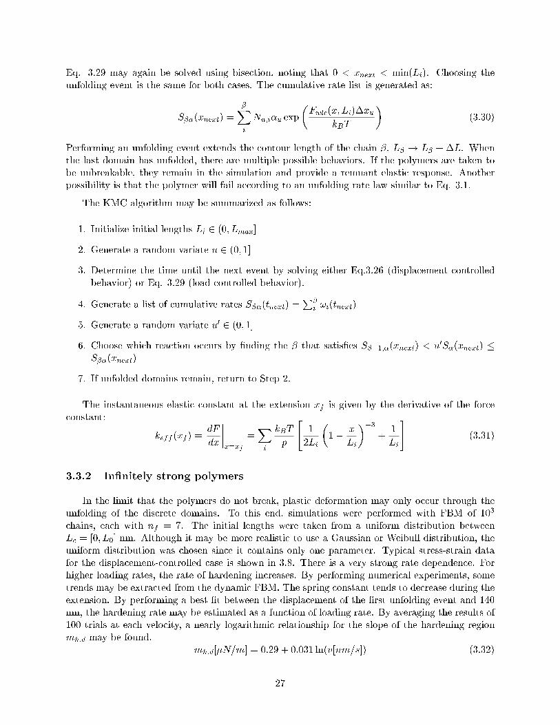
Eq. 3.29 may again be solved using bisection, noting that 0 < xnext < min(Li). Choosing theunfolding event is the same for both cases. The cumulative rate list is generated as:
S(xnext) =
Xi
Nu;iu exp
Fwlc(x; Li)xu
kBT
(3.30)
Performing an unfolding event extends the contour length of the chain , L ! L +L. Whenthe last domain has unfolded, there are multiple possible behaviors. If the polymers are taken tobe unbreakable, they remain in the simulation and provide a remnant elastic response. Anotherpossibility is that the polymer will fail according to an unfolding rate law similar to Eq. 3.1.
The KMC algorithm may be summarized as follows:
1. Initialize initial lengths Li 2 (0; Lmax]
2. Generate a random variate u 2 (0; 1]
3. Determine the time until the next event by solving either Eq.3.26 (displacement controlledbehavior) or Eq. 3.29 (load controlled behavior).
4. Generate a list of cumulative rates S(tnext) =P
i !i(tnext)
5. Generate a random variate u0 2 (0; 1]
6. Choose which reaction occurs by nding the that satises S1;(xnext) < u0S(xnext) S(xnext)
7. If unfolded domains remain, return to Step 2.
The instantaneous elastic constant at the extension xf is given by the derivative of the forceconstant:
keff (xf ) =dF
dx
x=xf
=Xi
kBT
p
"1
2Li
1 x
Li
3+
1
Li
#(3.31)
3.3.2 Innitely strong polymers
In the limit that the polymers do not break, plastic deformation may only occur through theunfolding of the discrete domains. To this end, simulations were performed with FBM of 103
chains, each with nf = 7. The initial lengths were taken from a uniform distribution betweenLc = [0; L0] nm. Although it may be more realistic to use a Gaussian or Weibull distribution, theuniform distribution was chosen since it contains only one parameter. Typical stress-strain datafor the displacement-controlled case is shown in 3.8. There is a very strong rate dependence. Forhigher loading rates, the rate of hardening increases. By performing numerical experiments, sometrends may be extracted from the dynamic FBM. The spring constant tends to decrease during theextension. By performing a best t between the displacement of the rst unfolding event and 140nm, the hardening rate may be estimated as a function of loading rate. By averaging the results of100 trials at each velocity, a nearly logarithmic relationship for the slope of the hardening regionmh;d may be found,
mh;d[N=m] = 0:29 + 0:031 ln(v[nm=s]) (3.32)
27
0 50 100Extension (nm)
0
20
40
60
80
100
Loa
d/ch
ain
(pN
)v=1000 nm/s
v=10
v=0.1
(a)
0 50 100Extension (nm)
0
4
8
12
k eff (
µN/m
)
v=1000 nm/s
v=10
v=0.1
(b)
Figure 3.8: Typical results of displacement-controlled KMC simulations of FBM. Panel 3.8a depictsthe load-displacement behavior for dierent values of the pulling velocity, v. The correspondingeective spring constants are shown in Panel 3.8b. In these simulations, N = 1000.
28

0.01 1 100 10000Loading rate (nm/s)
0
0.1
0.2
0.3
0.4
0.5
0.6m
(µN
/m)
(a)
0.01 1 100 10000Loading rate/chain (pN/s)
0.2
0.3
0.4
0.5
0.6
0.7
m (
µN/m
)
(b)
Figure 3.9: Slope of the hardening region for various values of loading rate for displacement-controlled deformation (Panel 3.9a) and load-controlled deformation (Panel 3.9b). Data points arethe average of 100 trials, with N = 100. The error bars are one standard deviation.
29
The results of the numerical simulation are shown in Fig. 3.9. The error bars on this plot arecalculated by taking the standard deviation of the slopes for the 100 trials.
The load-controlled simulations are performed at controlled values of =N0chains. Qualitatively,
the load-displacement behavior is quite similar, as seen in Fig. 3.10. For smaller values of theloading rate, the amount of softening is also smaller. Similarly to the displacement-controlledsimulations, the average slope of the hardening may also be calculated as a function of =N0
chains.The smoothness of the deformation, however, is strongly related to the deformation rates. Forfaster deformations, the load-displacement curve becomes increasingly jerky. Again, a logarithmicdependence of the hardening may be found:
mh;l[N=m] = 0:36 + 0:026 ln(=N0chains[pN=s]) (3.33)
3.3.3 Polymer failure
An alternate physical situation may be considered in which the polymers are allowed to failas well as break sacricial bonds. In the case that the polymer fails, it is necessary to denekinetic parameters for the failure event. There have not been experimental measurements of theseparameters, so in these simulations, the polymer is assumed to fail immediately after the naldomain unfolds.
Taking the initial number of chains to be N0chains, the load-controlled simulations are performed
at controlled values of =N0chains. Qualitatively, the load-displacement behavior is quite similar, as
seen in Fig. 3.9. For suciently small values of the loading rate, the bundle does not appreciablysoften. Similarly to the displacement-controlled simulations, the average slope of the hardeningmay also be calculated as a function of =N0
chains. The smoothness of the deformation, however, isstrongly related to the deformation rates.
Representative load-displacement curves are plotted in Fig. 3.11. These curves are very similarto those generated for innitely strong polymers. The more striking consequences of polymer failurecome from considering the strengths of the polymer bundles. The strengths are not uniform, butinstead follow a distribution that depends on the rate at which the bundle is deformed. To this end,bundles of 50 polymers were stressed until failure. Each polymer was taken to have 10 domains.103 trials were performed to nd the distribution of strengths. The results are plotted in Fig. 3.12.
Under load-controlled conditions, the stress on each polymer will increase as plastic eventsoccur. This will increase the stress on each polymer, causing correlations between plastic events.By analogy with dislocation plasticity, the size distributions of plastic events may be analyzed usinga scaling function analysis.
3.3.4 Distribution of plastic events
The distributions of time between plastic events were found to follow a power law, as shownin Fig. 3.13. Based on this observation, a scaling hypothesis may be made for n(a; t)da:dt, thenumber of plastic events where the extension to the next event falls between a and a+ da and thetime to the next event falls between t and t+ dt. The ansatz is
n(a; t) = n(a; t) (3.34)
30
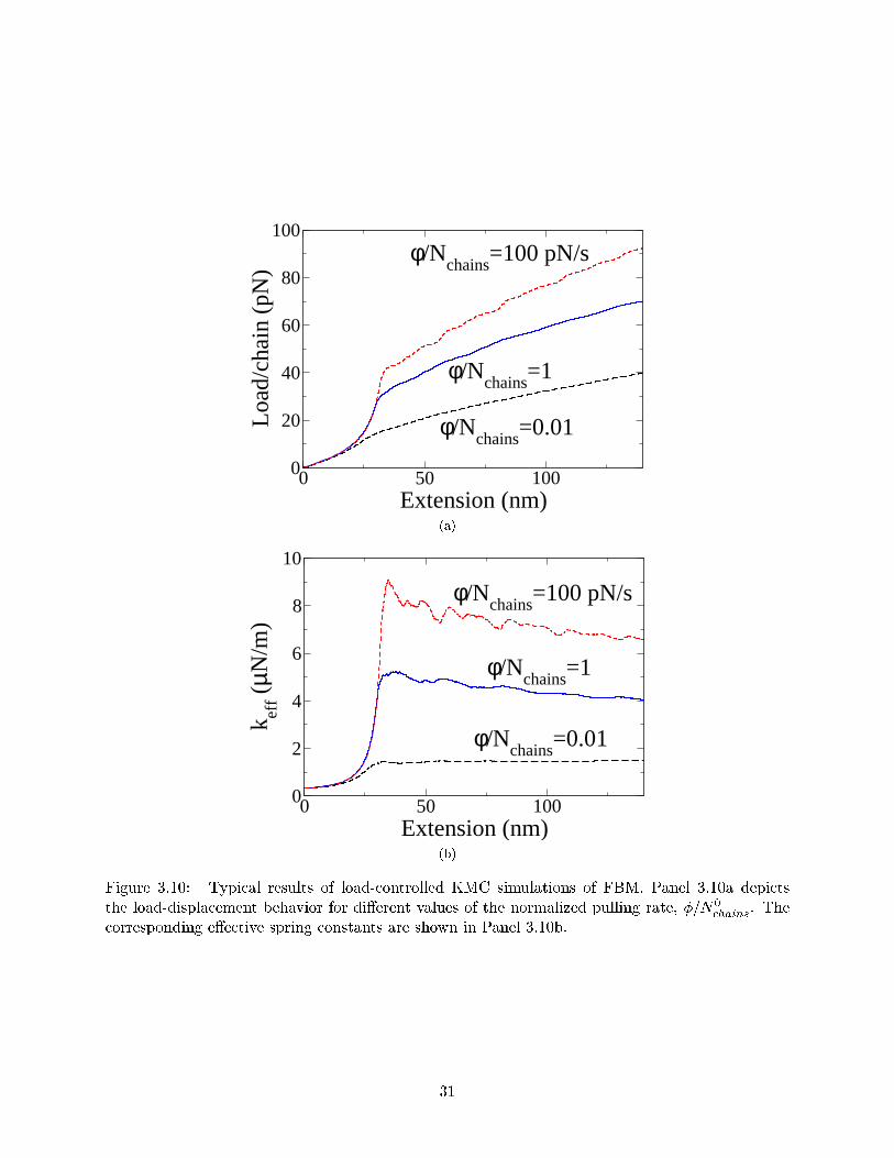
0 50 100Extension (nm)
0
20
40
60
80
100
Loa
d/ch
ain
(pN
)φ/N
chains=100 pN/s
φ/Nchains
=1
φ/Nchains
=0.01
(a)
0 50 100Extension (nm)
0
2
4
6
8
10
k eff (
µN/m
)
φ/Nchains
=100 pN/s
φ/Nchains
=1
φ/Nchains
=0.01
(b)
Figure 3.10: Typical results of load-controlled KMC simulations of FBM. Panel 3.10a depictsthe load-displacement behavior for dierent values of the normalized pulling rate, =N0
chains. Thecorresponding eective spring constants are shown in Panel 3.10b.
31
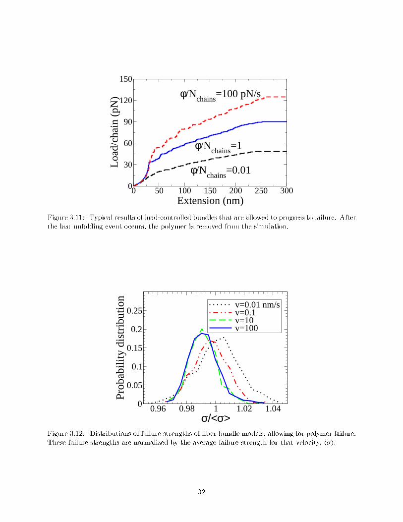
0 50 100 150 200 250 300Extension (nm)
0
30
60
90
120
150
Loa
d/ch
ain
(pN
) φ/Nchains
=100 pN/s
φ/Nchains
=1
φ/Nchains
=0.01
Figure 3.11: Typical results of load-controlled bundles that are allowed to progress to failure. Afterthe last unfolding event occurs, the polymer is removed from the simulation.
0.96 0.98 1 1.02 1.04σ/<σ>
0
0.05
0.1
0.15
0.2
0.25
Prob
abili
ty d
istr
ibut
ion
v=0.01 nm/sv=0.1v=10v=100
Figure 3.12: Distributions of failure strengths of ber bundle models, allowing for polymer failure.These failure strengths are normalized by the average failure strength for that velocity, hi.
32

100
101
102
103
Time between plastic events
10-6
10-4
10-2
100
Prob
abili
ty o
f pl
astic
eve
nt
Figure 3.13: Probability distribution of times between plastic events
where is an arbitrary constant, and and are the critical exponents of this transition. Inparticular, by taking = t1= , it may be shown that
t1=n(a; t) = n(t=a; 1) (3.35)
This expression is a function only of t=a. In other words, all data should collapse onto thesame curve, if plotted in terms of this parameter. Since Eq. 3.34 is chosen such that it re ectsscaling-law behavior in the time between plastic events and the size of the jump, it is possible tocalculate functions ~n(a) and ~n(l) from this analysis:
~n(l) =
Z 1
0n(l; a)da (3.36)
~n(a) =
Z 1
0n(l; a)dl (3.37)
The functions ~n(a) and ~n(l) are power laws. It is possible to demonstrate this by using the scalingansatz, then explicitly performing the integration.
~n(l) = 1Z 1
0n(l; a)da (3.38)
Choosing = l1=:
~n(l) = l1=Z 1
0n(1; l=a)da (3.39)
By performing the substitution x = l=a, dx = l=da, a power law is found:
~n(l) = l(1+)=Z 1
0n(1; x)dx (3.40)
with x = l=a and dx = l=da. The other exponent may be calculated similarly:
~n(a) = a(1+)=Z 1
0n(y; 1)dy (3.41)
33
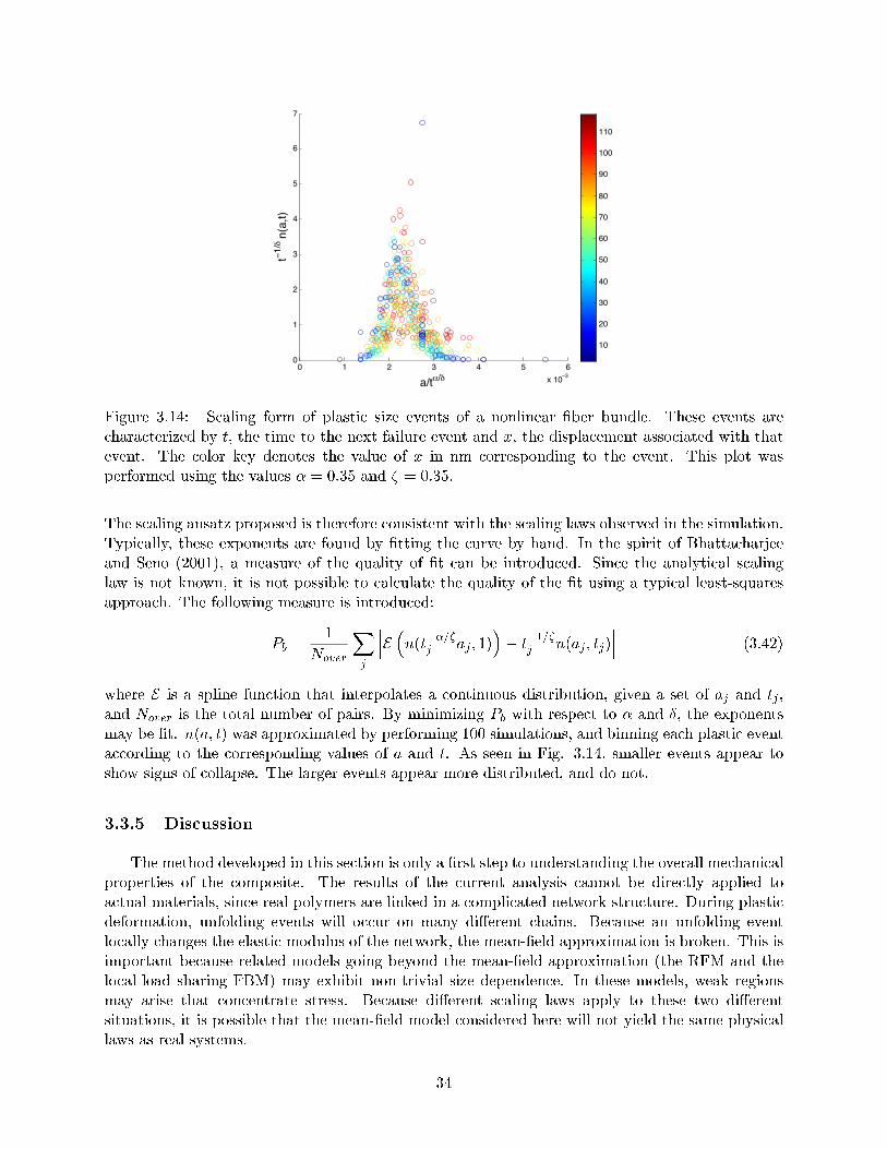
0 1 2 3 4 5 6x 10⁻³
0
1
2
3
4
5
6
7
a/tα/δ
t−1/δ n
(a,t)
10
20
30
40
50
60
70
80
90
100
110
Figure 3.14: Scaling form of plastic size events of a nonlinear ber bundle. These events arecharacterized by t, the time to the next failure event and x, the displacement associated with thatevent. The color key denotes the value of x in nm corresponding to the event. This plot wasperformed using the values = 0:35 and = 0:35.
The scaling ansatz proposed is therefore consistent with the scaling laws observed in the simulation.Typically, these exponents are found by tting the curve by hand. In the spirit of Bhattacharjeeand Seno (2001), a measure of the quality of t can be introduced. Since the analytical scalinglaw is not known, it is not possible to calculate the quality of the t using a typical least-squaresapproach. The following measure is introduced:
Pb =1
Nover
Xj
E n(t=j aj ; 1) t
1=j n(aj ; tj)
(3.42)
where E is a spline function that interpolates a continuous distribution, given a set of aj and tj ,and Nover is the total number of pairs. By minimizing Pb with respect to and , the exponentsmay be t. n(a; t) was approximated by performing 100 simulations, and binning each plastic eventaccording to the corresponding values of a and t. As seen in Fig. 3.14, smaller events appear toshow signs of collapse. The larger events appear more distributed, and do not.
3.3.5 Discussion
The method developed in this section is only a rst step to understanding the overall mechanicalproperties of the composite. The results of the current analysis cannot be directly applied toactual materials, since real polymers are linked in a complicated network structure. During plasticdeformation, unfolding events will occur on many dierent chains. Because an unfolding eventlocally changes the elastic modulus of the network, the mean-eld approximation is broken. This isimportant because related models going beyond the mean-eld approximation (the RFM and thelocal-load sharing FBM) may exhibit non-trivial size dependence. In these models, weak regionsmay arise that concentrate stress. Because dierent scaling laws apply to these two dierentsituations, it is possible that the mean-eld model considered here will not yield the same physicallaws as real systems.
34
The eect of the connectivity on the elastic response of network structures has been modeledusing techniques such as the eight-chain model (Arruda and Boyce, 1993). In this way, the responsefrom the WLC model may be related to a nonlinear elastic model (Ogden et al., 2006), such asthe Gent equation (Gent, 1996) or the Mooney-Rivlin model (Mooney, 1940; Rivlin, 1948). Inprinciple, the KMC algorithm presented here may be similarly modied to take spatial variationinto account. This is more dicult than the mean-eld problem addressed in this section. As anexample, consider a cubic array of NcNcNc nodes, connected by polymer chains. Connect thechains along the cube diagonals. The system is put under a uniform strain state, and the nodesare allowed to move around until no forces act on them. Consider each polymer chain to havesome number of folded states, unfolding with a rate determined by Eq. 3.25. In order to calculateP, it is necessary to solve 3 N3
c nonlinear equations at every integration step. This causes thecalculation of the cumulative rates to become computationally expensive. Although this calculationis feasible, it also motivates a desire to study models with simplied dynamics, as described in thenext chapter.
35
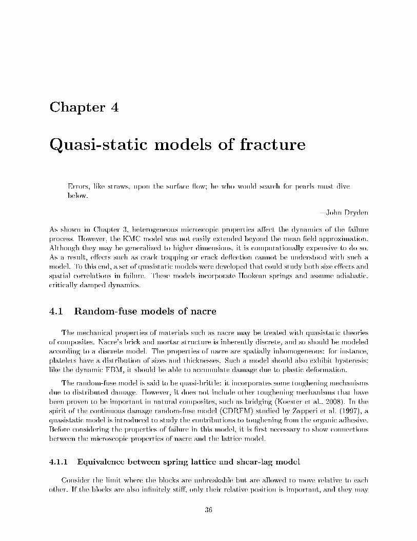
Chapter 4
Quasi-static models of fracture
Errors, like straws, upon the surface ow; he who would search for pearls must divebelow.
John Dryden
As shown in Chapter 3, heterogeneous microscopic properties aect the dynamics of the failureprocess. However, the KMC model was not easily extended beyond the mean-eld approximation.Although they may be generalized to higher dimensions, it is computationally expensive to do so.As a result, eects such as crack trapping or crack de ection cannot be understood with such amodel. To this end, a set of quasistatic models were developed that could study both size eects andspatial correlations in failure. These models incorporate Hookean springs and assume adiabatic,critically damped dynamics.
4.1 Random-fuse models of nacre
The mechanical properties of materials such as nacre may be treated with quasistatic theoriesof composites. Nacre's brick and mortar structure is inherently discrete, and so should be modeledaccording to a discrete model. The properties of nacre are spatially inhomogeneous: for instance,platelets have a distribution of sizes and thicknesses. Such a model should also exhibit hysteresis:like the dynamic FBM, it should be able to accumulate damage due to plastic deformation.
The random-fuse model is said to be quasi-brittle: it incorporates some toughening mechanismsdue to distributed damage. However, it does not include other toughening mechanisms that havebeen proven to be important in natural composites, such as bridging (Koester et al., 2008). In thespirit of the continuous damage random-fuse model (CDRFM) studied by Zapperi et al. (1997), aquasistatic model is introduced to study the contributions to toughening from the organic adhesive.Before considering the properties of failure in this model, it is rst necessary to show connectionsbetween the microscopic properties of nacre and the lattice model.
4.1.1 Equivalence between spring lattice and shear-lag model
Consider the limit where the blocks are unbreakable but are allowed to move relative to eachother. If the blocks are also innitely sti, only their relative position is important, and they may
36
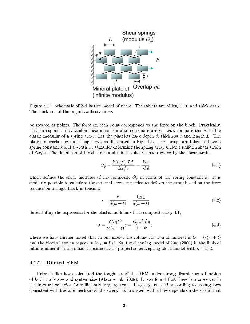
Shear springs
(modulus Gp)
Mineral platelet
(infinite modulus)
L
P
t
w
Overlap !L
Figure 4.1: Schematic of 2-d lattice model of nacre. The tablets are of length L and thickness t.The thickness of the organic adhesive is w.
be treated as points. The force on each point corresponds to the force on the block. Practically,this corresponds to a random fuse model on a tilted square array. Let's compare this with theelastic modulus of a spring array. Let the platelets have depth d, thickness t and length L. Theplatelets overlap by some length L, as illustrated in Fig. 4.1. The springs are taken to have aspring constant k and a width w. Consider deforming the spring array under a uniform shear strainof x=w. The denition of the shear modulus is the shear stress divided by the shear strain,
Gp =kx=(Ld)
x=w=
kw
Ld(4.1)
which denes the shear modulus of the composite Gp in terms of the spring constant k. It issimilarly possible to calculate the external stress needed to deform the array based on the forcebalance on a single block in tension:
=F
d(w + t)=
kx
d(w + t)(4.2)
Substituting the expression for the elastic modulus of the composite, Eq. 4.1,
=GpL
2
w(w + t) =
Gp22
1 (4.3)
where we have further noted that in our model the volume fraction of mineral is = t=(w + t)and the blocks have an aspect ratio = L=t. So, the shear-lag model of Gao (2006) in the limit ofinnite mineral stiness has the same elastic properties as a spring block model with = 1=2.
4.1.2 Diluted RFM
Prior studies have calculated the toughness of the RFM under strong disorder as a functionof both crack size and system size (Alava et al., 2008). It was found that there is a crossover inthe fracture behavior for suciently large systems. Large systems fail according to scaling lawsconsistent with fracture mechanics: the strength of a system with a aw depends on the size of that
37
aw. Small systems, however, are \notch-tolerant," and are independent of the size of the aw. Inother words, there is a transition observed in the toughness of RFMs depending on the crack size.
This may be understood similarly to the Gao criterion, discussed in Sec. 2.1.2. Under a certaincritical size, the inhomogeneities already present in the material will weaken the material. Underthis size, the material is notch-intolerant, and the strength of the sample will be determined bythe random nature of the material. One simple way to incorporate disorder into an RFM is toconstrain all springs to share the same fracture strength and modulus, but consider that only afraction p of the bonds are initially occupied. In the limit that p is close to 1, this is known as thediluted RFM, since there is only a small number of initially empty bonds.
The strength of the diluted model was calculated by Duxbury et al. (1987). They claimed that,similarly to cracks in brittle materials, the strength of the RFM is determined by the size of acritical aw. This defect must contain a critical number of broken bonds, nc. For a
pN pN
square lattice, this was found to be
nc lnN
ln(1 p)(4.4)
This criterion has consequences for materials that may be described by shear-lag theory. Consid-ering bricks with length L, and a total system size of Lsys = L
pN , it is possible to calculate the
size of a critical defect relative to the length of the block.
acL 2
lnL ln(Lsys)
ln(1 p)(4.5)
According to (Gao et al., 2003), the criterion for notch tolerance is set when the fracture strengthof a half-cracked sample is equal to the intrinsic strength of the material. This sets the maximumsystem size Lnt for which the sample is notch-tolerant. The strength of a half-cracked sample maybe calculated by setting ac=Lsys = 1=2,
1
2 L
Lnt2lnL ln(Lnt)
ln(1 p)(4.6)
This may be rearranged into the form
p 1 exp
4 L
LntlnLnt
L
(4.7)
Increasing the level of randomness increases the size of the cracks to which the material is notchinsensitive. However, it also decreases the strength of the system. This simple calculation predictsthat notch-tolerance is a property that is inherently dependent on the statistical distributions of themicroscopic properties. This suggests the importance of understanding the eect of distributionson other toughening mechanisms in nacre. This is explored in the following sections.
4.1.3 Modied CDRFM
As described in Section 2.1.3, the CDRFM was initially developed as a way to model plasticdeformation in heterogeneous materials. The elements are plastic in the sense that if one fails, it isreplaced with another fuse with a dierent spring constant. However, this microscopic plastic lawdoes not re ect the microscopic response of the organic adhesive.
38
Microscopic
hardeningNo hardening
Force
Extension
Damage
events
Figure 4.2: Diagram of microscopic plasticity laws utilized in the lattice model.
Considering the results of the KMC model described in Chapter 3, a microscopic plasticity lawshould be chosen that replicates the load-controlled response of the polymer. This is necessarybecause the blocks relax to a position in which they experience no force, even if the externalboundary condition is displacement controlled. Because the FBM exhibited hardening, the CDRFMmay be modied to have a yield strength that increases after each failure event. This behavior isillustrated schematically in Fig. 4.2
Estimates of the parameters may be extracted from the dynamic FBM. Some approximationsare made to simplify the lattice model. First, the elastic response is assumed to be linear. Sec-ond, damage is incorporated discretely: the spring constant is reduced by a constant factor atevery failure event. In the continuum limit, this is equivalent to the spring constant decreasingexponentially.
More formally, the algorithm may be described as follows. The ith spring is characterized byan initial stiness ki and an initial threshhold F
th;i. The spring network is expanded at a xedrate and the force on each spring is calculated to be Fs;i. The next spring to yield is selectedby nding the minimum Fth;i Fs;i. After the nth yield event, the stiness is reduced to beki(n) = anki , and the failure threshold is increased to be Fth;i(n) = F
th;i + b. For displacement-controlled loading conditions, the spring array will be subjected to a displacement vt, where v isthe externally imposed loading rate and t is the simulation time. The time to the breakage eventcan then be calculated from the force required to rupture that spring: Fth;i=vki. If this value issmaller than the current simulation time, the spring breakage event is taken to be part of a largerplastic event including multiple springs. If this value is larger than the current simulation time,the displacement is increased to Fth; i=ki and the process repeats.
Spatial extent of damage
In order to understand how fracture processes are aected by the local microscopic laws, it isimportant to understand how damage spreads during deformation. In particular, it is importantto understand under what conditions damage localizes into a well-dened crack. This is done byconsidering the deformation of 32 32 element lattices, using Fth = 1, k = 1 and a = 0:9. Theamount of hardening was calculated for dierent values of b.
The progressive yielding of the springs may be visualized with a contour plot of the numberof yield events experienced by the dierent springs. This is plotted for dierent, representative
39
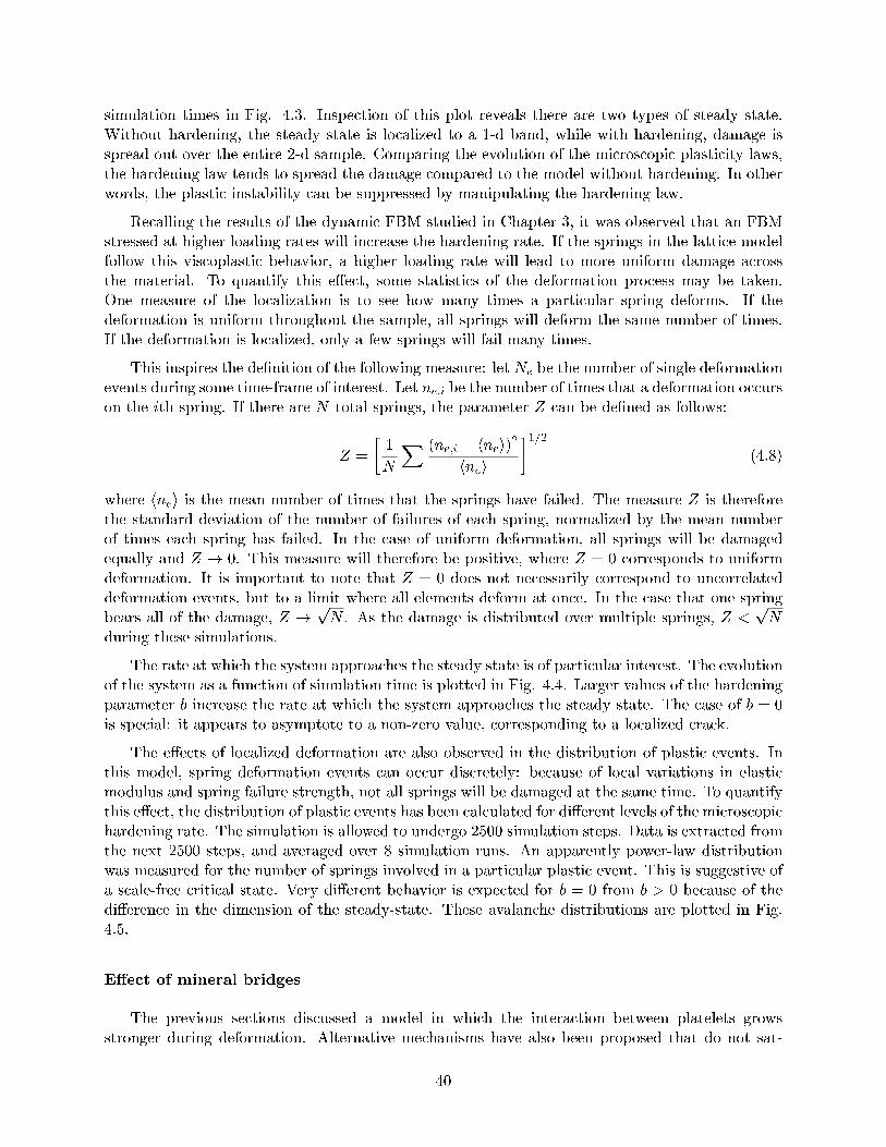
simulation times in Fig. 4.3. Inspection of this plot reveals there are two types of steady state.Without hardening, the steady state is localized to a 1-d band, while with hardening, damage isspread out over the entire 2-d sample. Comparing the evolution of the microscopic plasticity laws,the hardening law tends to spread the damage compared to the model without hardening. In otherwords, the plastic instability can be suppressed by manipulating the hardening law.
Recalling the results of the dynamic FBM studied in Chapter 3, it was observed that an FBMstressed at higher loading rates will increase the hardening rate. If the springs in the lattice modelfollow this viscoplastic behavior, a higher loading rate will lead to more uniform damage acrossthe material. To quantify this eect, some statistics of the deformation process may be taken.One measure of the localization is to see how many times a particular spring deforms. If thedeformation is uniform throughout the sample, all springs will deform the same number of times.If the deformation is localized, only a few springs will fail many times.
This inspires the denition of the following measure: let Ne be the number of single deformationevents during some time-frame of interest. Let ne;i be the number of times that a deformation occurson the ith spring. If there are N total springs, the parameter Z can be dened as follows:
Z =
1
N
X (ne;i hnei)2hnei
1=2(4.8)
where hnei is the mean number of times that the springs have failed. The measure Z is thereforethe standard deviation of the number of failures of each spring, normalized by the mean numberof times each spring has failed. In the case of uniform deformation, all springs will be damagedequally and Z ! 0. This measure will therefore be positive, where Z = 0 corresponds to uniformdeformation. It is important to note that Z = 0 does not necessarily correspond to uncorrelateddeformation events, but to a limit where all elements deform at once. In the case that one springbears all of the damage, Z ! p
N . As the damage is distributed over multiple springs, Z <pN
during these simulations.
The rate at which the system approaches the steady state is of particular interest. The evolutionof the system as a function of simulation time is plotted in Fig. 4.4. Larger values of the hardeningparameter b increase the rate at which the system approaches the steady state. The case of b = 0is special: it appears to asymptote to a non-zero value, corresponding to a localized crack.
The eects of localized deformation are also observed in the distribution of plastic events. Inthis model, spring deformation events can occur discretely: because of local variations in elasticmodulus and spring failure strength, not all springs will be damaged at the same time. To quantifythis eect, the distribution of plastic events has been calculated for dierent levels of the microscopichardening rate. The simulation is allowed to undergo 2500 simulation steps. Data is extracted fromthe next 2500 steps, and averaged over 8 simulation runs. An apparently power-law distributionwas measured for the number of springs involved in a particular plastic event. This is suggestive ofa scale-free critical state. Very dierent behavior is expected for b = 0 from b > 0 because of thedierence in the dimension of the steady-state. These avalanche distributions are plotted in Fig.4.5.
Eect of mineral bridges
The previous sections discussed a model in which the interaction between platelets growsstronger during deformation. Alternative mechanisms have also been proposed that do not sat-
40
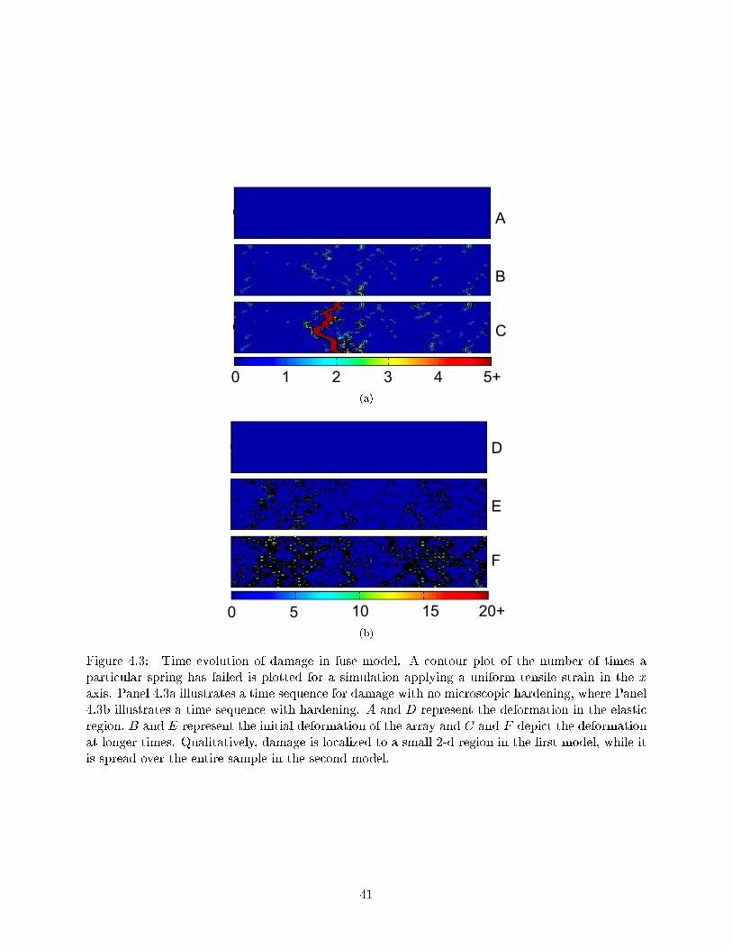
0 1 2 3 4 5+
A
B
C
(a)
0 5 10 15 20+
D
E
F
(b)
Figure 4.3: Time evolution of damage in fuse model. A contour plot of the number of times aparticular spring has failed is plotted for a simulation applying a uniform tensile strain in the xaxis. Panel 4.3a illustrates a time sequence for damage with no microscopic hardening, where Panel4.3b illustrates a time sequence with hardening. A and D represent the deformation in the elasticregion, B and E represent the initial deformation of the array and C and F depict the deformationat longer times. Qualitatively, damage is localized to a small 2-d region in the rst model, while itis spread over the entire sample in the second model.
41
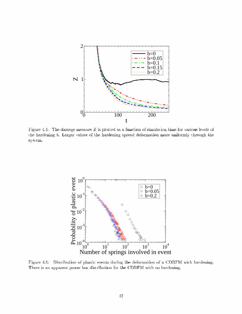
0 100 200t
0
1
2
Z
b=0b=0.05b=0.1b=0.15b=0.2
Figure 4.4: The damage measure Z is plotted as a function of simulation time for various levels ofthe hardening b. Larger values of the hardening spread deformation more uniformly through thesystem.
100
101
102
103
104
Number of springs involved in event
10-4
10-3
10-2
10-1
100
Prob
abili
ty o
f pl
astic
eve
nt
b=0b=0.05b=0.2
Figure 4.5: Distribution of plastic events during the deformation of a CDRFM with hardening.There is an apparent power law distribution for the CDRFM with no hardening.
42
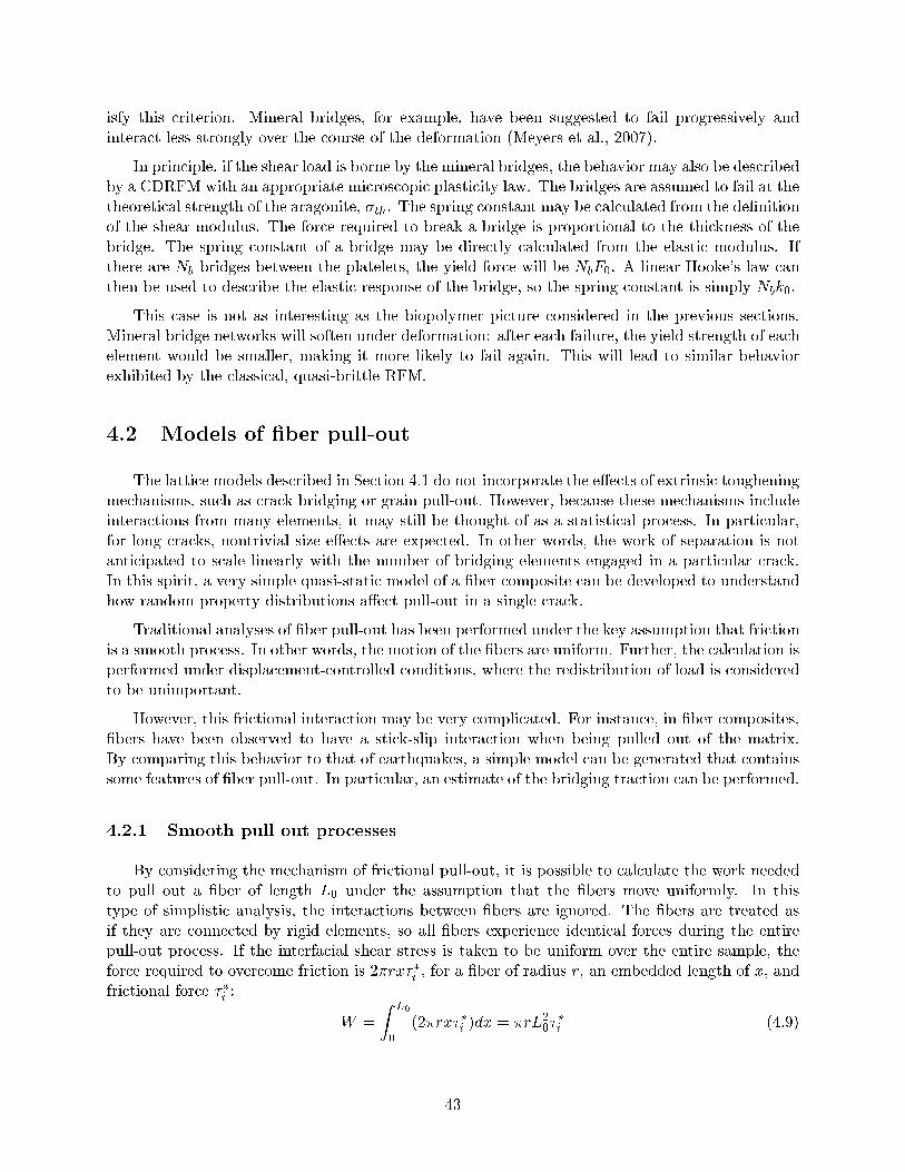
isfy this criterion. Mineral bridges, for example, have been suggested to fail progressively andinteract less strongly over the course of the deformation (Meyers et al., 2007).
In principle, if the shear load is borne by the mineral bridges, the behavior may also be describedby a CDRFM with an appropriate microscopic plasticity law. The bridges are assumed to fail at thetheoretical strength of the aragonite, th. The spring constant may be calculated from the denitionof the shear modulus. The force required to break a bridge is proportional to the thickness of thebridge. The spring constant of a bridge may be directly calculated from the elastic modulus. Ifthere are Nb bridges between the platelets, the yield force will be NbF0. A linear Hooke's law canthen be used to describe the elastic response of the bridge, so the spring constant is simply Nbk0.
This case is not as interesting as the biopolymer picture considered in the previous sections.Mineral bridge networks will soften under deformation: after each failure, the yield strength of eachelement would be smaller, making it more likely to fail again. This will lead to similar behaviorexhibited by the classical, quasi-brittle RFM.
4.2 Models of ber pull-out
The lattice models described in Section 4.1 do not incorporate the eects of extrinsic tougheningmechanisms, such as crack bridging or grain pull-out. However, because these mechanisms includeinteractions from many elements, it may still be thought of as a statistical process. In particular,for long cracks, nontrivial size eects are expected. In other words, the work of separation is notanticipated to scale linearly with the number of bridging elements engaged in a particular crack.In this spirit, a very simple quasi-static model of a ber composite can be developed to understandhow random property distributions aect pull-out in a single crack.
Traditional analyses of ber pull-out has been performed under the key assumption that frictionis a smooth process. In other words, the motion of the bers are uniform. Further, the calculation isperformed under displacement-controlled conditions, where the redistribution of load is consideredto be unimportant.
However, this frictional interaction may be very complicated. For instance, in ber composites,bers have been observed to have a stick-slip interaction when being pulled out of the matrix.By comparing this behavior to that of earthquakes, a simple model can be generated that containssome features of ber pull-out. In particular, an estimate of the bridging traction can be performed.
4.2.1 Smooth pull out processes
By considering the mechanism of frictional pull-out, it is possible to calculate the work neededto pull out a ber of length L0 under the assumption that the bers move uniformly. In thistype of simplistic analysis, the interactions between bers are ignored. The bers are treated asif they are connected by rigid elements, so all bers experience identical forces during the entirepull-out process. If the interfacial shear stress is taken to be uniform over the entire sample, theforce required to overcome friction is 2rxi , for a ber of radius r, an embedded length of x, andfrictional force i :
W =
Z L0
0(2rxi )dx = rL2
0i (4.9)
43
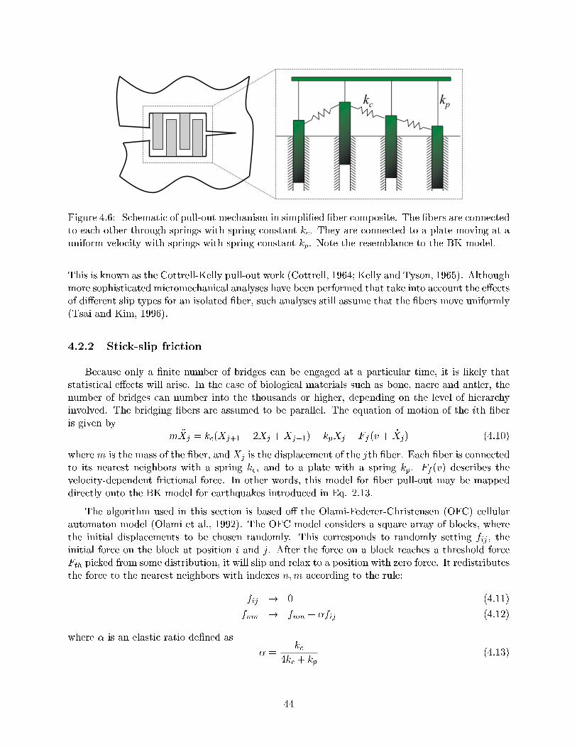
kpkc
Figure 4.6: Schematic of pull-out mechanism in simplied ber composite. The bers are connectedto each other through springs with spring constant kc. They are connected to a plate moving at auniform velocity with springs with spring constant kp. Note the resemblance to the BK model.
This is known as the Cottrell-Kelly pull-out work (Cottrell, 1964; Kelly and Tyson, 1965). Althoughmore sophisticated micromechanical analyses have been performed that take into account the eectsof dierent slip types for an isolated ber, such analyses still assume that the bers move uniformly(Tsai and Kim, 1996).
4.2.2 Stick-slip friction
Because only a nite number of bridges can be engaged at a particular time, it is likely thatstatistical eects will arise. In the case of biological materials such as bone, nacre and antler, thenumber of bridges can number into the thousands or higher, depending on the level of hierarchyinvolved. The bridging bers are assumed to be parallel. The equation of motion of the ith beris given by
m Xj = kc(Xj+1 2Xj +Xj1) kpXj Ff (v + _Xj) (4.10)
wherem is the mass of the ber, and Xj is the displacement of the jth ber. Each ber is connectedto its nearest neighbors with a spring kc, and to a plate with a spring kp. Ff (v) describes thevelocity-dependent frictional force. In other words, this model for ber pull-out may be mappeddirectly onto the BK model for earthquakes introduced in Eq. 2.13.
The algorithm used in this section is based o the Olami-Federer-Christensen (OFC) cellularautomaton model (Olami et al., 1992). The OFC model considers a square array of blocks, wherethe initial displacements to be chosen randomly. This corresponds to randomly setting fij , theinitial force on the block at position i and j. After the force on a block reaches a threshold forceFth picked from some distribution, it will slip and relax to a position with zero force. It redistributesthe force to the nearest neighbors with indexes n;m according to the rule:
fij ! 0 (4.11)
fnm ! fnm + fij (4.12)
where is an elastic ratio dened as
=kc
4kc + kp(4.13)
44
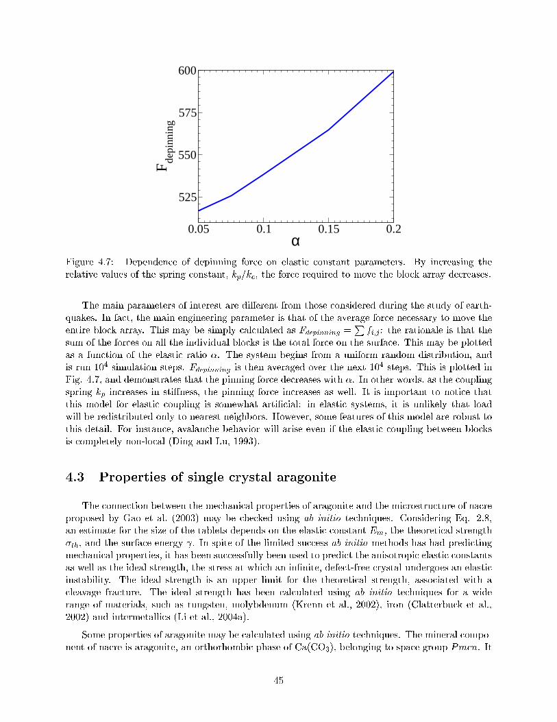
0.05 0.1 0.15 0.2α
525
550
575
600
F depi
nnin
g
Figure 4.7: Dependence of depinning force on elastic constant parameters. By increasing therelative values of the spring constant, kp=kc, the force required to move the block array decreases.
The main parameters of interest are dierent from those considered during the study of earth-quakes. In fact, the main engineering parameter is that of the average force necessary to move theentire block array. This may be simply calculated as Fdepinning =
Pfi;j : the rationale is that the
sum of the forces on all the individual blocks is the total force on the surface. This may be plottedas a function of the elastic ratio . The system begins from a uniform random distribution, andis run 104 simulation steps. Fdepinning is then averaged over the next 104 steps. This is plotted inFig. 4.7, and demonstrates that the pinning force decreases with . In other words, as the couplingspring kp increases in stiness, the pinning force increases as well. It is important to notice thatthis model for elastic coupling is somewhat articial: in elastic systems, it is unlikely that loadwill be redistributed only to nearest neighbors. However, some features of this model are robust tothis detail. For instance, avalanche behavior will arise even if the elastic coupling between blocksis completely non-local (Ding and Lu, 1993).
4.3 Properties of single crystal aragonite
The connection between the mechanical properties of aragonite and the microstructure of nacreproposed by Gao et al. (2003) may be checked using ab initio techniques. Considering Eq. 2.8,an estimate for the size of the tablets depends on the elastic constant Em, the theoretical strengthth, and the surface energy . In spite of the limited success ab initio methods has had predictingmechanical properties, it has been successfully been used to predict the anisotropic elastic constantsas well as the ideal strength, the stress at which an innite, defect-free crystal undergoes an elasticinstability. The ideal strength is an upper limit for the theoretical strength, associated with acleavage fracture. The ideal strength has been calculated using ab initio techniques for a widerange of materials, such as tungsten, molybdenum (Krenn et al., 2002), iron (Clatterbuck et al.,2002) and intermetallics (Li et al., 2004a).
Some properties of aragonite may be calculated using ab initio techniques. The mineral compo-nent of nacre is aragonite, an orthorhombic phase of Ca(CO3), belonging to space group Pmcn. It
45
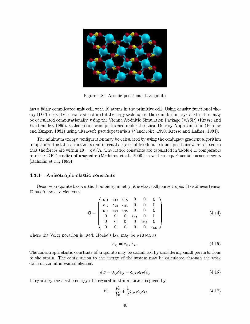
Figure 4.8: Atomic positions of aragonite.
has a fairly complicated unit cell, with 10 atoms in the primitive cell. Using density functional the-ory (DFT) based electronic structure total energy techniques, the equilibrium crystal structure maybe calculated computationally, using the Vienna Ab-initio Simulation Package (VASP) (Kresse andFurthmuller, 1996). Calculations were performed under the Local Density Approximation (Perdewand Zunger, 1981) using ultra-soft pseudopotentials (Vanderbilt, 1990; Kresse and Hafner, 1994).
The minimum energy conguration may be calculated by using the conjugate gradient algorithmto optimize the lattice constants and internal degrees of freedom. Atomic positions were relaxed sothat the forces are within 106 eV=A. The lattice constants are tabulated in Table 4.1, comparableto other DFT studies of aragonite (Medeiros et al., 2006) as well as experimental measurements(Balmain et al., 1999)
4.3.1 Anisotropic elastic constants
Because aragonite has a orthorhombic symmetry, it is elastically anisotropic. Its stiness tensorC has 9 nonzero elements.
C =
0BBBBBB@
c11 c12 c13 0 0 0c12 c22 c23 0 0 0c13 c23 c33 0 0 00 0 0 c44 0 00 0 0 0 c55 00 0 0 0 0 c66
1CCCCCCA
(4.14)
where the Voigt notation is used. Hooke's law may be written as
ij = cijklkl: (4.15)
The anisotropic elastic constants of aragonite may be calculated by considering small perturbationsto the strain. The contribution to the energy of the system may be calculated through the workdone on an innitesimal element
dw = ijdij = cijklkldij (4.16)
Integrating, the elastic energy of a crystal in strain state is given by
FV =F0V0
+1
2cijklijkl (4.17)
46
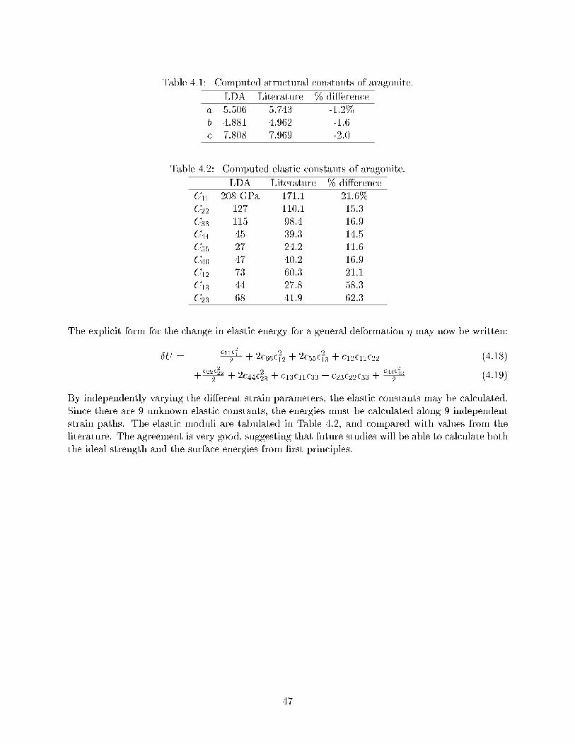
Table 4.1: Computed structural constants of aragonite.
LDA Literature % dierence
a 5.506 5.743 -1.2%b 4.881 4.962 -1.6c 7.808 7.969 -2.0
Table 4.2: Computed elastic constants of aragonite.
LDA Literature % dierence
C11 208 GPa 171.1 21.6%C22 127 110.1 15.3C33 115 98.4 16.9C44 45 39.3 14.5C55 27 24.2 11.6C66 47 40.2 16.9C12 73 60.3 21.1C13 44 27.8 58.3C23 68 41.9 62.3
The explicit form for the change in elastic energy for a general deformation may now be written:
U =c11211
2 + 2c66212 + 2c55
213 + c121122 (4.18)
+c22222
2 + 2c44223 + c131133 + c232233 +
c332332 (4.19)
By independently varying the dierent strain parameters, the elastic constants may be calculated.Since there are 9 unknown elastic constants, the energies must be calculated along 9 independentstrain paths. The elastic moduli are tabulated in Table 4.2, and compared with values from theliterature. The agreement is very good, suggesting that future studies will be able to calculate boththe ideal strength and the surface energies from rst principles.
47
Chapter 5
Models of microstructural evolution
Everything's got a moral, if only you can nd it.
Lewis Carroll
5.1 Rayleigh instability in hollow-core dislocations
The energy of a hollow-core dislocation may be separated into surface, elastic, and chemicalcomponents. Following Frank (1951) and Cahn (1957), the free energy of a cylindrically symmetrichollow-core dislocation may be represented by a functional that depends on the radius, R(z),
F [R(z)] =
Z
0dz
8<:2 R
"1 +
@R
@z
2#1=2
A logR fR2
9=; ; (5.1)
where is the surface energy and f is taken to be the volumetric free energy of formation of thevoid. The A logR term corresponds to the elastic energy relieved from the presence of the void.The value of A depends on the character of the dislocation: A = Gb2=4(1) for edge dislocationsand A = Gb2=4 for screw dislocations. G and are the shear modulus and Poisson's ratio of thematrix, and b is the length of the Burgers' vector of the dislocation. Formally, the system must benite in size: otherwise, the elastic energy of the system diverges. For computational simplicity, thematrix is considered to be a cylinder of radius Rmat, centered around the hollow-core dislocation.
Frank (1951) considered Eq. 5.1 in the limit of isotropic surface energy, and set f = 0. Underthese conditions, the energy per unit length of a cylinder radius R is given by
FL(R) = 2 RA logR (5.2)
If mass is not conserved, the free energy is minimized for dislocations of a critical radius, R =A=2 . This prediction for the equilibrium size of a hollow-core dislocation is known as Frank'sradius.
5.1.1 Thermodynamic analysis
Consider a single, initially cylindrical hollow-core dislocation with radius R0. Using Eq. 5.1, itis possible to calculate the increase in free energy from a sinusoidal perturbation with wavelength
48
, F = FperturbedFperfect. Choosing uctuations that conserve mass, the radius is chosen to bea function of z in the form
R(z; t) = R1 + (t) cos(2z=) (5.3)
where (t) is taken to be small compared to R0. The value of R1 is set by a mass conservationcondition. The volume of the perturbed cylinder is taken to be equal to that of the unperturbedcylinder for a single period of the sinusoid.
Vunperturbed = Vperturbed (5.4)
R20 =
Z
0[R1 + (t) cos(2z=)]2dz (5.5)
Eq. 5.5 sets the constraint on R1 that R20 R2
1 = 2=2. Following Cahn (1979), is takento be anisotropic in the direction of the dislocation line. The geometry of the system remainsaxisymmetric, and is a function only of the angle = @R=@z. may be expanded about as
() = 0 + 0 +1
22 00 +O(3); (5.6)
where 0 = @ =@ and 00 = @2 =@2. F may be calculated by combining Eq. 5.1, Eq. 5.3 andEq. 5.6. Keeping only terms of order 2,
F =
A2
2R20
2R0+23R0
+23R0
002: (5.7)
A hollow-core dislocation is unstable to perturbations that cause the free energy to decrease relativeto Fperfect. The condition F < 0 is true for values of which satisfy:
> 2(R0)3=2
s 0 + 00
R0 0 A: (5.8)
In the limit that R ! 0 and 00 ! 0, this expression reduces to the classical Rayleigh (1878)condition, > isotropicmin = 2R0. The form of Eq. 5.8 suggests that it is useful to dene a scalingparameter S,
S =
s1 + 00= 01 2R=R0
(5.9)
which contains contributions from both surface-energy anisotropy as well as elastic energy fromthe dislocation. Fig. 5.1 explores the relationship between these two parameters, plotting S fordierent values of 00= 0 over a range of R0=R
.
Using this denition, it is easy to show that there is a minimum unstable wavelength min =isotropicmin S. A cylindrical hollow-core dislocation will be unstable to perturbations with wavelength > min. Conversely, perturbations with wavelength shorter than the minimum wavelength willdecay.
5.1.2 Kinetic analysis
The main result of the thermodynamic analysis is an expression for min, the minimum allowedwavelength for Rayleigh break-up. It is not a prediction for the observed periodicity of the insta-bility. This is a dicult problem, which would require direct simulation of the microstructure. To
49
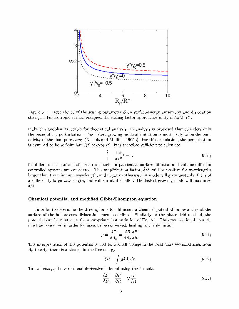
2 4 6 8 10R
0/R*
0
1
2
3
4
Sγ’’/γ0=0.5
γ’’/γ0=−0.5γ’’/γ0=0
Figure 5.1: Dependence of the scaling parameter S on surface-energy anisotropy and dislocationstrength. For isotropic surface energies, the scaling factor approaches unity if R0 R.
make this problem tractable for theoretical analysis, an analysis is proposed that considers onlythe onset of the perturbation. The fastest-growing mode at initiation is most likely to be the peri-odicity of the nal pore array (Nichols and Mullins, 1965b). For this calculation, the perturbationis assumed to be self-similar: (t) / exp(t). It is therefore sucient to calculate
_
1
@
@t = (5.10)
for dierent mechanisms of mass transport. In particular, surface-diusion and volume-diusioncontrolled systems are considered. This amplication factor, _=, will be positive for wavelengthslarger than the minimum wavelength, and negative otherwise. A mode will grow unstably if it is ofa suciently large wavelength, and will shrink if smaller. The fastest-growing mode will maximize_=.
Chemical potential and modied Gibbs-Thompson equation
In order to determine the driving force for diusion, a chemical potential for vacancies at thesurface of the hollow-core dislocation must be dened. Similarly to the phase-eld method, thepotential can be related to the appropriate rst variation of Eq. 5.1. The cross-sectional area Ax
must be conserved in order for mass to be conserved, leading to the denition
=F
Ax=
R
Ax
F
R(5.11)
The interpretation of this potential is that for a small change in the local cross sectional area, fromAx to Ax, there is a change in the free energy
F =
ZAxdz (5.12)
To evaluate , the variational derivative is found using the formula
F
R=@F
@RrF
R(5.13)
50
In the one-dimensional problem considered here, r @@z . For a circular cross-section, Ax = R2
and so (R=Ax) = (@Ax=@R)1 = (2R)1.
=1
2R
8><>:2
"1 +
@R
@z
2#1=2
A
R 2fR @
@z2R
@R@zh
1 +@R@z
2i1=29>=>; (5.14)
For innitesimal perturbations, only terms of rst order in @R=@z must be retained. The linearizedpotential is then:
= 0R 0 + 00
@2R@z2
A
2R2 f (5.15)
This form of the chemical potential has consequences for the Gibbs-Thompson eect. The localsolubility must also be aected by surface-energy anisotropy and strain energy. To quantitativelycalculate this eect, an additional assumption is made, that vacancies do not interact elasticallyeither with the dislocation strain eld or with each other. It is also necessary to choose a referencestate for the enrichment in solubility. This is taken to be a cylindrical hollow-core dislocation withradius Rref . The dierence in chemical potential between the reference state and the system withan arbitrary prole R(z) is:
= (R; dR=dz) (Rref ; 0) = 0R
0 + 00
@2R@z2
A
2R2 0Rref
+A
2R2ref
(5.16)
where is the molar volume of the vacancy. The transfer of dn moles of material from the referencestate to the system of interest causes an increase in free energy
dG = dn: (5.17)
Eq. 5.17 is true locally: it is valid at every point z. The free energy change may then be denedas:
= GB(R; dR=dz) GB(Rref ; 0) = kBT logaB(R; dR=dz)
aB(Rref ; 0)(5.18)
where GB(R; dR=dz) is the partial molar free energy and aB(R; dR=dz) is the activity of the vacancy.In the dilute-solution limit, aB = cB. According to Henry's law, the activity coecient isindependent of concentration and so:
= kBT logcB(R; dR=dz)
cB(Rref ; 0)(5.19)
After solving for cB(R; dR=dz) and linearizing:
cB(R; dR=dz) = cB(Rref ; 0) exp
kBT cB(Rref ; 0)
1 +
kBT
(5.20)
Dening the local enrichment to be c = cB(R; dR=dz) cB(Rref ; 0),
c =cB(Rref ; 0)
kBT
0R 0 + 00
@2R@z2
0R
R2 0Rref
+ 0R
R2ref
!(5.21)
If the reference state is chosen to be suciently large, the nal terms of Eq. 5.21 vanish. In thecase that R Rref Rmat, cB(Rref ; 0) approaches c0, the equilibrium concentration at a at
51

interface, in the absence of dislocations. For this choice of reference state, the modied form of theGibbs-Thompson relationship is:
c =c0
kBT
0R 0 + 00
@2R@z2
0R
R2
(5.22)
In the limit of surface-energy isotropy and in the absence of a dislocation, Eq. 5.22 reduces to theclassical Gibbs-Thompson equation.
Surface diusion
Mullins (1957) proposed a general expression for the normal velocity of the surface @n=@t dueto surface diusion
@n
@t=DsNsr2
s
kBT(5.23)
where Ds is the surface diusion coecient, and the rs is the surface Laplacian. A combinationof Eq. 5.15 and Eq. 5.23 may be used to determine the evolution of the innitesimally perturbedcylinder described by Eq. 5.3. Keeping only terms of order , the chemical potential is
= 0R0
0 cos!z
R20
+ 0 + 00
!2 cos!z A
2R20
+A cos!z
R30
f (5.24)
where ! = 2=. For small perturbations, s z, and the surface Laplacian becomesr2s = (@2=@z2).
The velocity of the surface is then given by
@n
@t= B!2
1
R20
0 !2 0 + 00
02R
R30
cos!z (5.25)
where B = (DsNs)=(kBT ). Another expression for the surface velocity may be found by dier-entiating Eq. 5.3 with respect to time.
@n
@t=@R
@t= _ cos!z (5.26)
By comparing Eq. 5.25 and 5.26, an expression for the amplication factor _= may be found tobe
_
= B!2
1
R20
0 !2 0 + 00
02R
R30
: (5.27)
Volume diusion
When volume diusion governs the Rayleigh instability, the amplication factor may be foundby solving Fick's Laws using Eq. 5.22 as a boundary condition. Considering a perturbed hollow-core dislocation with prole described by Eq. 5.3, the change in solubility at the surface of thedislocation is:
c =c0 0kBT
1
R0 cos!z
R20
+1 + 00= 0
!2 cos!z R
R20
+2R cos!z
R30
(5.28)
52

to rst order in . The steady-state concentration must satisfy Laplace's equation, r2c = 0. Forthe case of cylindrical symmetry, the general solution is:
c = fA0I0(!r) +B0K0(!r)gfC sin!z +D cos!zg+ E (5.29)
where I0(z) is the modied Bessel function of the rst kind of order 0, K0(z) is the modiedBessel function of the second kind of order 0, and A0, B0, C, and E are constants set by theboundary conditions. To determine the value of these constants, multiple distinct situations thatcan be analyzed. Two situations are \external" volume diusion, where volume diusion throughthe matrix is the dominant transport mechanism, and \internal" volume diusion, where volumediusion in the hollow-core dislocation is dominant.
Under normal conditions, the core of a hollow-core dislocation is empty, and so internal volumediusion is not physically meaningful. However, this case is applicable to the more general situation,where the core is lled with an arbitrary phase. This is the case if a second-phase cylindricalprecipitate is formed on a dislocation. A formal treatment of this microstructure is more dicultthan the current one of a hollow-core dislocation: in particular, elastic eects from the interfacecomplicate the analysis. However, if the mismatch is not large, it should have the similar genericbehavior to the present case.
In the case of external volume diusion, it is necessary to consider the vacancy concentrationoutside of the cylinder. I0(z) diverges as z !1, forcing A0 = 0. Since the perturbation chosen isproportional to cos!z, C = 0. Then, only two parameters are free, and the concentration is set bythe equation:
c = B00K0(!r) cos!z + E (5.30)
The modied Gibbs-Thompson equation sets the value of this equation at the cylinder surface,r = R. By comparison to Eq. 5.28, the constants may be set as:
B00 =1
K0(!R0)
c0 0kBT
1
R20
+1 + 00= 0
!2 +
R
R30
(5.31)
E =c0 0kBT
1
R0 R
R20
(5.32)
so the solution for the concentration eld for all space is:
c =c0 0kBT
1 + 00= 0
!2 1
R20
+2R
R30
K0(!r)
K0(!R0) cos!z +
1
R0 R
R20
(5.33)
Assuming that growth is diusion limited, the rate at which vacancies are transported to the surfaceof the hollow-core dislocation will determine the rate at which the perturbation grows. Using Fick'srst law, which relates mass ux to concentration gradients, the vacancy ux into the dislocationmay be calculated. The radial component of the vacancy ux, evaluated at the surface of thehollow-core dislocation, is
Jr =
D@c
@r
r=R0+ cos!
(5.34)
where D is the lattice diusion coecient. The normal velocity of the surface is proportional toJr.
@n
@t=dr
dt= J =
D2c0 0!
kBT
1
R20
2R
R30
1 + 00= 0!2
K1(!r)
K0(!R0) cos!z (5.35)
53
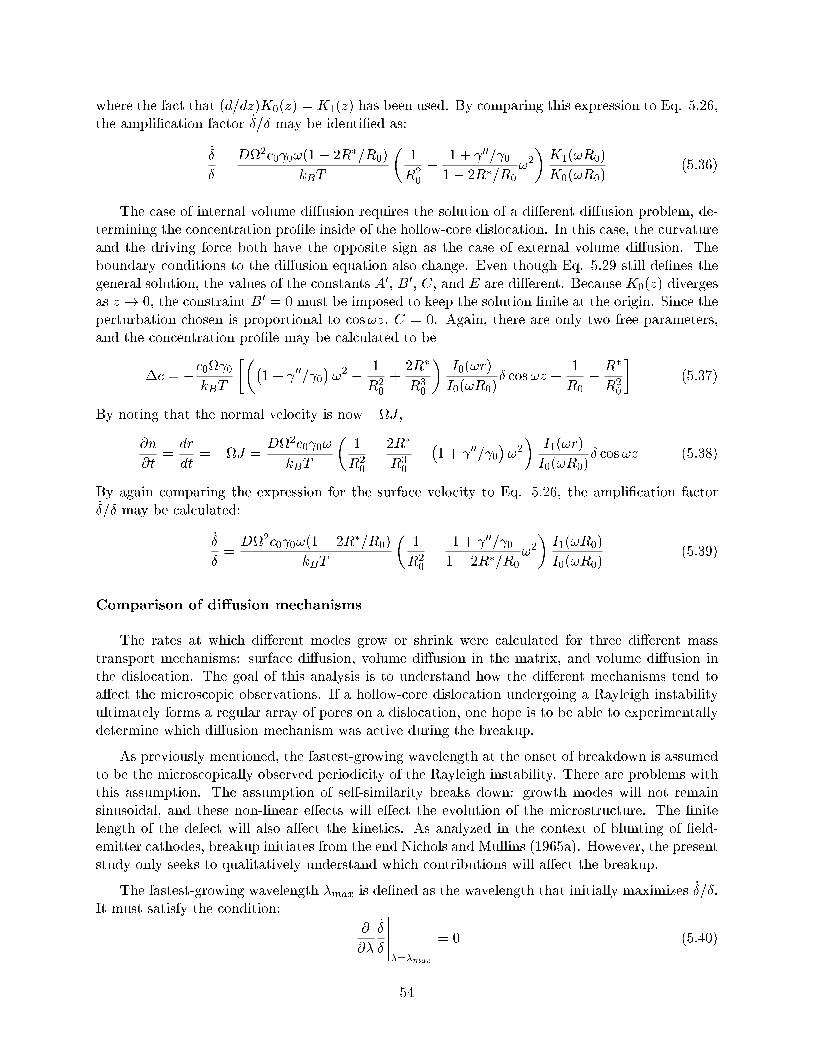
where the fact that (d=dz)K0(z) = K1(z) has been used. By comparing this expression to Eq. 5.26,the amplication factor _= may be identied as:
_
=D2c0 0!(1 2R=R0)
kBT
1
R20
1 + 00= 01 2R=R0
!2K1(!R0)
K0(!R0)(5.36)
The case of internal volume diusion requires the solution of a dierent diusion problem, de-termining the concentration prole inside of the hollow-core dislocation. In this case, the curvatureand the driving force both have the opposite sign as the case of external volume diusion. Theboundary conditions to the diusion equation also change. Even though Eq. 5.29 still denes thegeneral solution, the values of the constants A0, B0, C, and E are dierent. Because K0(z) divergesas z ! 0, the constraint B0 = 0 must be imposed to keep the solution nite at the origin. Since theperturbation chosen is proportional to cos!z, C = 0. Again, there are only two free parameters,and the concentration prole may be calculated to be
c = c0 0kBT
1 + 00= 0
!2 1
R20
+2R
R30
I0(!r)
I0(!R0) cos!z +
1
R0 R
R20
(5.37)
By noting that the normal velocity is now J ,@n
@t=dr
dt= J =
D2c0 0!
kBT
1
R20
2R
R30
1 + 00= 0!2
I1(!r)
I0(!R0) cos!z (5.38)
By again comparing the expression for the surface velocity to Eq. 5.26, the amplication factor_= may be calculated:
_
=D2c0 0!(1 2R=R0)
kBT
1
R20
1 + 00= 01 2R=R0
!2I1(!R0)
I0(!R0)(5.39)
Comparison of diusion mechanisms
The rates at which dierent modes grow or shrink were calculated for three dierent masstransport mechanisms: surface diusion, volume diusion in the matrix, and volume diusion inthe dislocation. The goal of this analysis is to understand how the dierent mechanisms tend toaect the microscopic observations. If a hollow-core dislocation undergoing a Rayleigh instabilityultimately forms a regular array of pores on a dislocation, one hope is to be able to experimentallydetermine which diusion mechanism was active during the breakup.
As previously mentioned, the fastest-growing wavelength at the onset of breakdown is assumedto be the microscopically observed periodicity of the Rayleigh instability. There are problems withthis assumption. The assumption of self-similarity breaks down: growth modes will not remainsinusoidal, and these non-linear eects will eect the evolution of the microstructure. The nitelength of the defect will also aect the kinetics. As analyzed in the context of blunting of eld-emitter cathodes, breakup initiates from the end Nichols and Mullins (1965a). However, the presentstudy only seeks to qualitatively understand which contributions will aect the breakup.
The fastest-growing wavelength max is dened as the wavelength that initially maximizes _=.It must satisfy the condition:
@
@
_
=max
= 0 (5.40)
54
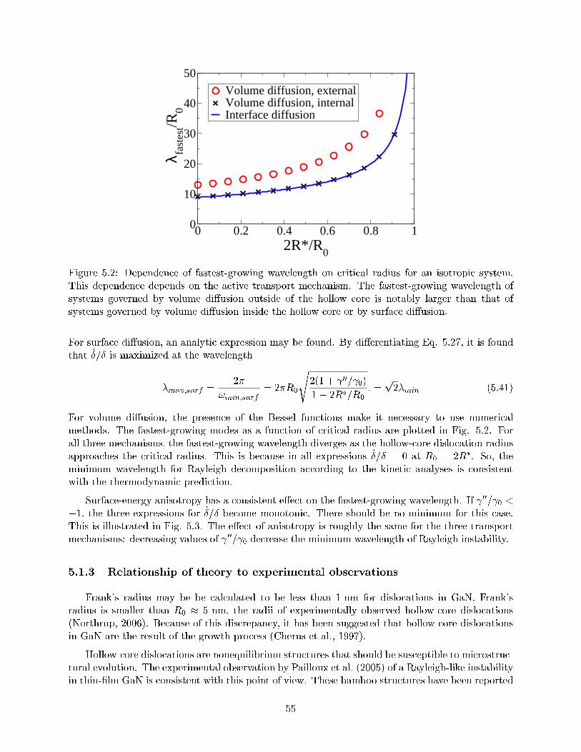
0 0.2 0.4 0.6 0.8 12R*/R
0
0
10
20
30
40
50
λ fast
est/R
0
Volume diffusion, externalVolume diffusion, internalInterface diffusion
Figure 5.2: Dependence of fastest-growing wavelength on critical radius for an isotropic system.This dependence depends on the active transport mechanism. The fastest-growing wavelength ofsystems governed by volume diusion outside of the hollow core is notably larger than that ofsystems governed by volume diusion inside the hollow core or by surface diusion.
For surface diusion, an analytic expression may be found. By dierentiating Eq. 5.27, it is foundthat _= is maximized at the wavelength
max;surf =2
!min;surf= 2R0
s2(1 + 00= 0)
1 2R=R0: =
p2min (5.41)
For volume diusion, the presence of the Bessel functions make it necessary to use numericalmethods. The fastest-growing modes as a function of critical radius are plotted in Fig. 5.2. Forall three mechanisms, the fastest-growing wavelength diverges as the hollow-core dislocation radiusapproaches the critical radius. This is because in all expressions _= = 0 at R0 = 2R. So, theminimum wavelength for Rayleigh decomposition according to the kinetic analyses is consistentwith the thermodynamic prediction.
Surface-energy anisotropy has a consistent eect on the fastest-growing wavelength. If 00= 0 <1, the three expressions for _= become monotonic. There should be no minimum for this case.This is illustrated in Fig. 5.3. The eect of anisotropy is roughly the same for the three transportmechanisms: decreasing values of 00= 0 decrease the minimum wavelength of Rayleigh instability.
5.1.3 Relationship of theory to experimental observations
Frank's radius may be be calculated to be less than 1 nm for dislocations in GaN. Frank'sradius is smaller than R0 5 nm, the radii of experimentally observed hollow-core dislocations(Northrup, 2006). Because of this discrepancy, it has been suggested that hollow-core dislocationsin GaN are the result of the growth process (Cherns et al., 1997).
Hollow-core dislocations are nonequilibrium structures that should be susceptible to microstruc-tural evolution. The experimental observation by Pailloux et al. (2005) of a Rayleigh-like instabilityin thin-lm GaN is consistent with this point of view. These bamboo structures have been reported
55
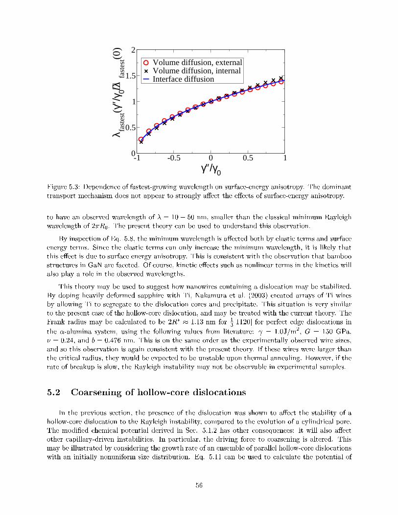
-1 -0.5 0 0.5 1γ″/γ0
0
0.5
1
1.5
2
λ fast
est(γ
″/γ0)/λ
fast
est(0
)
Volume diffusion, externalVolume diffusion, internalInterface diffusion
Figure 5.3: Dependence of fastest-growing wavelength on surface-energy anisotropy. The dominanttransport mechanism does not appear to strongly aect the eects of surface-energy anisotropy.
to have an observed wavelength of = 10 50 nm, smaller than the classical minimum Rayleighwavelength of 2R0. The present theory can be used to understand this observation.
By inspection of Eq. 5.8, the minimum wavelength is aected both by elastic terms and surfaceenergy terms. Since the elastic terms can only increase the minimum wavelength, it is likely thatthis eect is due to surface energy anisotropy. This is consistent with the observation that bamboostructures in GaN are faceted. Of course, kinetic eects such as nonlinear terms in the kinetics willalso play a role in the observed wavelengths.
This theory may be used to suggest how nanowires containing a dislocation may be stabilized.By doping heavily deformed sapphire with Ti, Nakamura et al. (2003) created arrays of Ti wiresby allowing Ti to segregate to the dislocation cores and precipitate. This situation is very similarto the present case of the hollow-core dislocation, and may be treated with the current theory. TheFrank radius may be calculated to be 2R 1:13 nm for 1
3 [1120] for perfect edge dislocations in
the -alumina system, using the following values from literature: = 1:0J/m2, G = 150 GPa, = 0:24, and b = 0:476 nm. This is on the same order as the experimentally observed wire sizes,and so this observation is again consistent with the present theory. If these wires were larger thanthe critical radius, they would be expected to be unstable upon thermal annealing. However, if therate of breakup is slow, the Rayleigh instability may not be observable in experimental samples.
5.2 Coarsening of hollow-core dislocations
In the previous section, the presence of the dislocation was shown to aect the stability of ahollow-core dislocation to the Rayleigh instability, compared to the evolution of a cylindrical pore.The modied chemical potential derived in Sec. 5.1.2 has other consequences: it will also aectother capillary-driven instabilities. In particular, the driving force to coarsening is altered. Thismay be illustrated by considering the growth rate of an ensemble of parallel hollow-core dislocationswith an initially nonuniform size distribution. Eq. 5.11 can be used to calculate the potential of
56
0 1 2 3 4 5R/2R*
0
0.5
2R*µ
/Ωγ
Figure 5.4: Chemical potential of point defects at the surface of the dislocation core as a functionof dislocation radius. The chemical potential is normalized by =2R. There is a maximum whenthe particle radius is twice the Frank radius.
point defects about the ith dislocation,
i = A
2R2i
+
Ri=
R
R
2
R2i
+R
Ri
(5.42)
where the ith dislocation has radius Ri. This potential is plotted in Fig. 5.4. Eq. 5.42 illustratesthat the local growth rate is aected by the presence of the dislocation. If all hollow-core dislocationsare able to exchange mass with each other, the growth rate of a particular dislocation will dependon the sizes of the other dislocations. Under a mean-eld assumption, the driving force for thegrowth of the ith wire is driven by the dierence of the chemical potential of the particular wirewith the average chemical potential, = i . The average chemical potential of the systemis given by =
Pj j . It is important to note that even though a local particle growth law may
be calculated, and continuity is observed, a LSW-style analysis is not valid. The eects of thedislocation becomes less important as rods grow in size. The existence of an internal length scaleensures that the asymptotic state does not exist, since spatial self-similarity cannot be observed induring coarsening.
It possible to determine some tendencies of this ensemble of hollow-core dislocations. Considera distribution where the largest dislocation has a diameter smaller than 2R. The slope of thepotential is positive for all of the dislocations in the ensemble. This means that dislocations largerthan the critical radius will have a positive chemical potential dierence, and will tend to shrink.The interpretation of Eq. 5.42 is that there will be inverse coarsening when the largest dislocationhas a diameter smaller than 2R. Therefore, if the ensemble of hollow-core dislocations is sucientlysmall, the system will tend to focus the dislocation sizes.
This limit for thermodynamic stability is dierent from Frank's radius. This is because theboundary conditions considered for coarsening are dierent from the situation studied by Frank(1951). Frank considered the case that the mass of a particular wire is allowed to uctuate, whilethe mass of the ensemble of wires is xed to be constant in the coarsening problem.
57
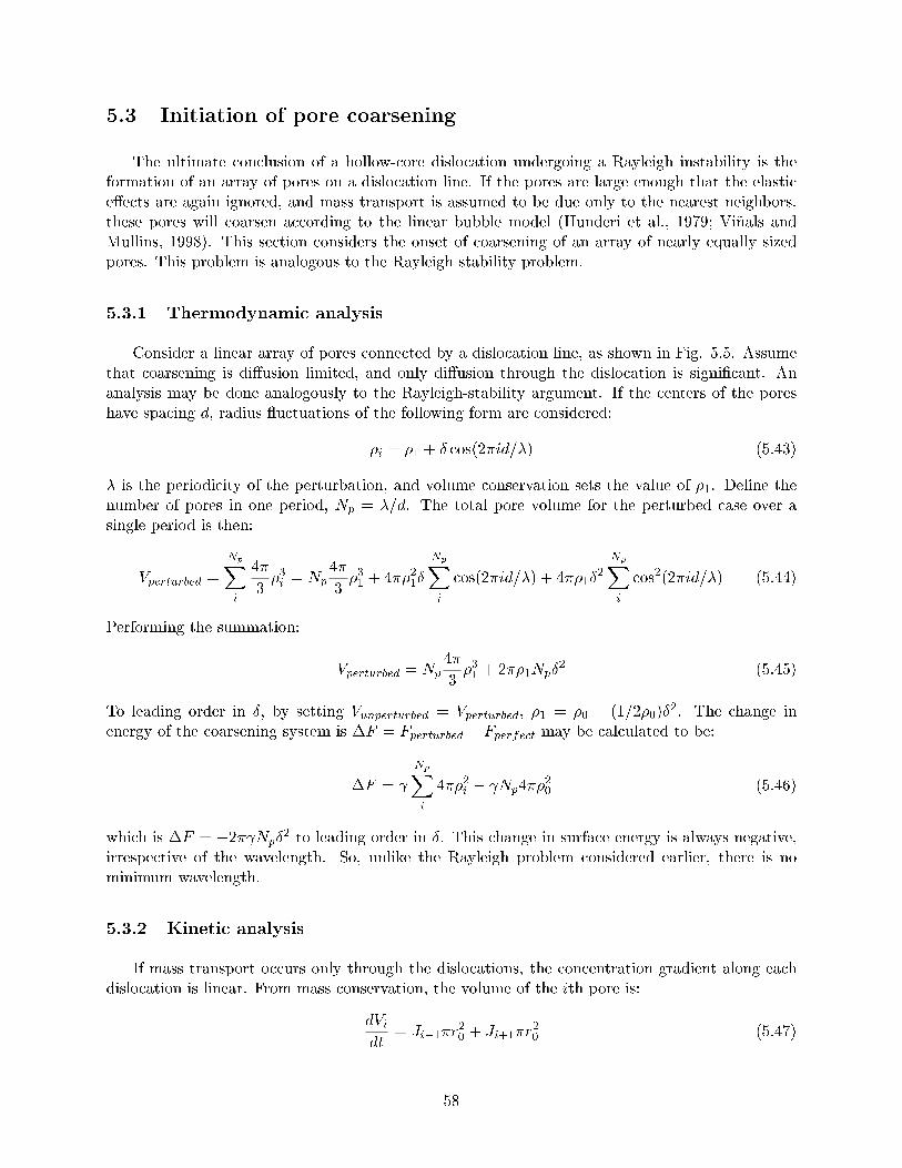
5.3 Initiation of pore coarsening
The ultimate conclusion of a hollow-core dislocation undergoing a Rayleigh instability is theformation of an array of pores on a dislocation line. If the pores are large enough that the elasticeects are again ignored, and mass transport is assumed to be due only to the nearest neighbors,these pores will coarsen according to the linear bubble model (Hunderi et al., 1979; Vi~nals andMullins, 1998). This section considers the onset of coarsening of an array of nearly equally sizedpores. This problem is analogous to the Rayleigh stability problem.
5.3.1 Thermodynamic analysis
Consider a linear array of pores connected by a dislocation line, as shown in Fig. 5.5. Assumethat coarsening is diusion limited, and only diusion through the dislocation is signicant. Ananalysis may be done analogously to the Rayleigh-stability argument. If the centers of the poreshave spacing d, radius uctuations of the following form are considered:
i = 1 + cos(2id=) (5.43)
is the periodicity of the perturbation, and volume conservation sets the value of 1. Dene thenumber of pores in one period, Np = =d. The total pore volume for the perturbed case over asingle period is then:
Vperturbed =
NpXi
4
33i = Np
4
331 + 421
NpXi
cos(2id=) + 412
NpXi
cos2(2id=) (5.44)
Performing the summation:
Vperturbed = Np4
331 + 21Np
2 (5.45)
To leading order in , by setting Vunperturbed = Vperturbed, 1 = 0 (1=20)2. The change in
energy of the coarsening system is F = Fperturbed Fperfect may be calculated to be:
F =
NpXi
42i Np420 (5.46)
which is F = 2 Np2 to leading order in . This change in surface energy is always negative,
irrespective of the wavelength. So, unlike the Rayleigh problem considered earlier, there is nominimum wavelength.
5.3.2 Kinetic analysis
If mass transport occurs only through the dislocations, the concentration gradient along eachdislocation is linear. From mass conservation, the volume of the ith pore is:
dVidt
= Ji1r20 + Ji+1r
20 (5.47)
58
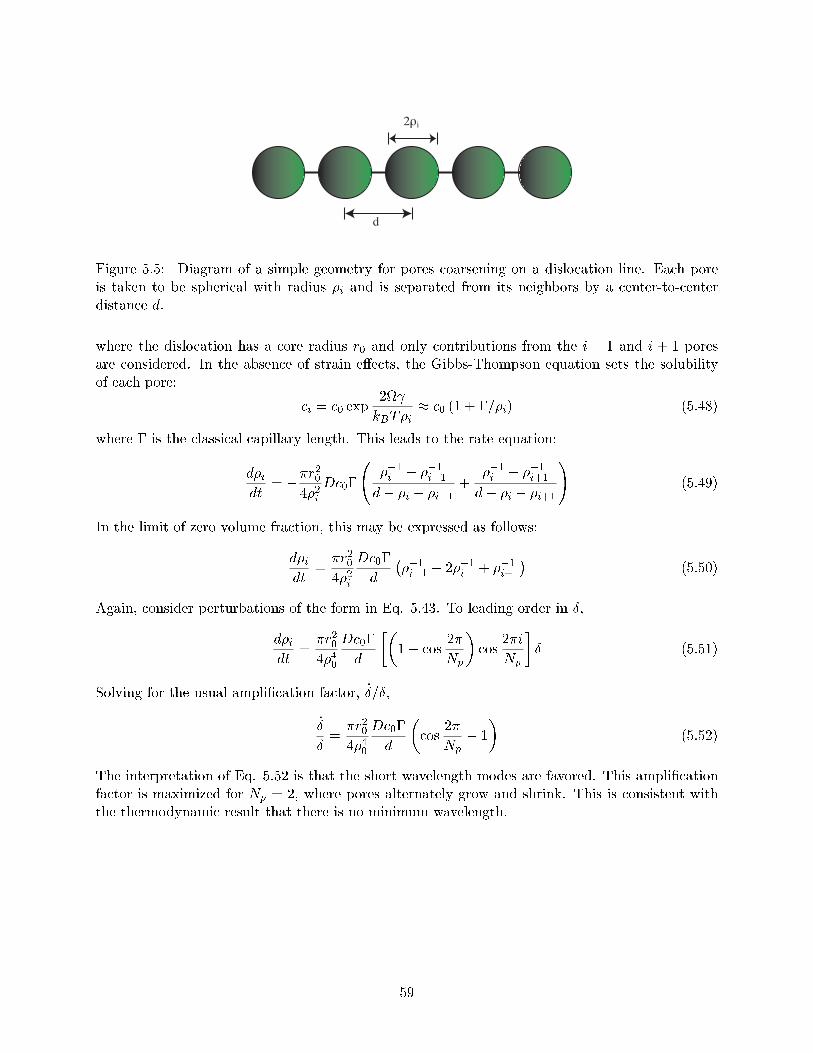
2ρi
d
Figure 5.5: Diagram of a simple geometry for pores coarsening on a dislocation line. Each poreis taken to be spherical with radius i and is separated from its neighbors by a center-to-centerdistance d.
where the dislocation has a core radius r0 and only contributions from the i 1 and i + 1 poresare considered. In the absence of strain eects, the Gibbs-Thompson equation sets the solubilityof each pore:
ci = c0 exp2
kBTi c0 (1 + =i) (5.48)
where is the classical capillary length. This leads to the rate equation:
didt
= r20
42iDc0
1i 1i1d i i1
+1i 1i+1d i i+1
!(5.49)
In the limit of zero volume fraction, this may be expressed as follows:
didt
=r2042i
Dc0
d
1i1 21i + 1i+1
(5.50)
Again, consider perturbations of the form in Eq. 5.43. To leading order in ,
didt
=r20440
Dc0
d
1 cos
2
Np
cos
2i
Np
(5.51)
Solving for the usual amplication factor, _=,
_
=r20440
Dc0
d
cos
2
Np 1
(5.52)
The interpretation of Eq. 5.52 is that the short wavelength modes are favored. This amplicationfactor is maximized for Np = 2, where pores alternately grow and shrink. This is consistent withthe thermodynamic result that there is no minimum wavelength.
59
Chapter 6
Closing remarks
The truth is rarely pure and never simple.
Oscar Wilde
Two types of strain-mediated instabilities were studied in this thesis. In Chapters 3 and 4, statisticalmechanics techniques were used to study the fracture of heterogeneous systems. In Chapter 5, theevolution of a model microstructure due to instabilities from surface energy was considered. Therole of strain energy is very dierent for the two examples studied. While strain is the driving forcefor fracture in composites, it tends to stabilize the capillary instability in hollow-core dislocations.
6.1 Deformation of nacre
The toughening mechanisms in nacre were considered using both quasi-static and time-dependent treatments. Because of the statistical nature of the models studied, size eects arenaturally expected to arise. The deformation of nacre-like materials was studied using kineticMonte Carlo techniques and direct integration in the adiabatic limit. The biopolymer was ana-lyzed using a two state model for the deformation of a class of biopolymers under the rare eventlimit assuming irreversible kinetics. An algorithm was presented that allows calculation of themechanical properties under various loading conditions. Analytical results for the force at rstunfolding were found in the limit that unfolding is irreversible. The energy dispersed during un-folding is calculated to be a large fraction of the work needed to extend the system. This modelwas further extended to ensembles of polymer chains.
In some sense, the microscopic disorder is a way to characterize the fracture toughness of thesystem. These models may be slightly modied to other natural materials. Bone, for instance, alsohas a hierarchical structure that involves toughening mechanisms on many length scales. Similarlyto lustrin A in nacre, the matrix proteins osteopontin (Fantner et al., 2007) and dentin matrixprotein 1 (Adams et al., 2008) have been suggested to exhibit the same behavior. There are twoimportant possible extensions to this model. First, the assumption of irreversible kinetics may berelaxed by incorporating refolding events. Further, the bundle geometry may be extended to morerealistic congurations.
60

6.2 Structural stability of hollow-core dislocations
The susceptibility of the hollow-core dislocation to the Rayleigh instability and coarsening wasstudied, focusing on only leading-order eects. By assuming a self-similar evolution, analytical ex-pressions were derived that determined a critical radius for the stability of hollow-core dislocations.A parameter S( 00= 0; R
=R0) was identied that summarizes the interplay between surface-energyanisotropy and strain energy. By analogy to precipitate formation, this suggests a path for thefabrication of a stable nanowire array.
However, a more detailed calculation would need to treat both the interface and the pointdefects more carefully. In a precipitate, the interface may be coherent, aecting the strain energyof the system. Point defects will also interact elastically, in principle changing the Gibbs-Thompsonequation. Further, the transport equations used are simplistic: they are only true for the simplecase of vacancy self-diusion in a metal.
In order to deal with the case of diusion in a ceramic, diusion currents of multiple speciesmust be considered. Since the various point defects have dierent charges associated with them,these currents will be strongly coupled. Likewise, the interfaces may develop a local space charge.This causes point defects to tend to arrange themselves to minimize the total energy of the system.
However, even by including these physical eects, the linear stability analysis cannot give acomplete understanding of the behavior. For instance, it is not obvious if the growth of the Rayleighinstability is bounded. In other words, it is not clear if an unstable hollow-core dislocation willeventually pinch-o. Further, the nite size of real dislocations may play an important role in theultimate break up of the rods. To study these aspects of Eq. 5.23, it is possible to consider the fullevolution equation
@n
@t=DsNs
kBTr2s
8><>:2
h1 +
@R@z
2 R@2R@z2
ih1 +
@R@z
2i3=2 A
R
9>=>; (6.1)
By solving this equation numerically, it should be possible to determine the time evolution of thehollow-core dislocation. This equation of motion is consistent with existing theories: in the limitthat A = 0, this equation is identical to that considered by Nichols and Mullins (1965a).
61
Bibliography
Adams, J., Fantner, G. E., Fisher, L. W., Hansma, P. K., 2008. Molecular energy dissipation innanoscale networks of dentin matrix protein 1 is strongly dependent on ion valence. Nanotech-nology 19, 17.
Alava, M. J., Nukala, P. K. V. V., Zapperi, S., 2006. Statistical models of fracture. Advances inPhysics 55 (3), 349476.
Alava, M. J., Nukala, P. K. V. V., Zapperi, S., 2008. Role of disorder in the size scaling of materialstrength. Physical Review Letters 100, 055502.
Ardell, A. J., 1972. Isotropic ber coarsening in unidirectional solidied eutectic alloys. Metallur-gical Transactions 3 (6), 1395.
Arruda, E. M., Boyce, M. C., 1993. A three-dimensional constitutive model for the large stretchbehavior of rubber elastic materials. Journal of the Mechanics and Physics of Solids 41 (2),389412.
Bahr, D. F., Kramer, D. E., Gerberich, W. W., 1998. Non-linear deformation mechanisms duringnanoindentation. Acta Materialia 46, 3605.
Balk, J., Lukac, P., 1993. Portevin-Le Chatelier instabilities in Al-3 Mg conditioned by strain rateand strain. Acta Metallurgica et Materialia 41 (5), 14471454.
Balmain, J., Hannoyer, B., Lopez, E., 1999. Fourier transform infrared spectroscopy (FTIR) andx-ray diraction analyses of mineral and organic matric during heating of mother of pearl (nacre)from the shell of the molusc Pinctada maxima. Journal of Biomedical Materials Research 48 (5),749.
Barenblatt, G. I., 2003. Scaling. Cambridge University Press.
Barthelat, F., Tang, H., Zavattieri, P., Li, C.-M., Espinosa, H., 2006. On the mechanics of mother-of-pearl: A key feature in the material hierarchical structure. Journal of the Mechanics andPhysics of Solids 55 (2), 306337.
Bhattacharjee, S. M., Seno, F., 2001. A measure of data collapse for scaling. Journal of Physics A:Mathematical and General 34, 63756380.
Bonderer, L. J., Studart, A. R., Gauckler, L. J., 2008. Bioinspired design and assembly of plateletreinforced polymer lms. Science 319, 10691073.
Brailsford, A. D., Wynblatt, P., 1979. The dependence of Ostwald ripening kinetics on particlevolume fraction. Acta Metallurgica 27, 489.
62
Burridge, R., Knopo, L., 1967. Model and theoretical seismicity. Bulletin of the SeismologicalSociety of America 57 (3), 341.
Cabrera, N., Levine, M. M., 1956. On the dislocation theory of evaporation of crystals. PhilosophicalMagazine 1 (5), 450458.
Cahn, J. W., 1957. Nucleation on dislocations. Acta Metallurgica 5, 169172.
Cahn, J. W., 1979. Stability of rods with anisotropic surface free energy. Scripta Metallurgica 13,10691071.
Carlson, J. M., Langer, J. S., 1989. Mechanical model of an earthquake fault. Physical Review A40 (11), 64706484.
Carlson, J. M., Langer, J. S., Shaw, B. E., 1994. Dynamics of earthquake faults. Reviews of ModernPhysics 66 (2), 657671.
Cherns, D., 2000. The structure and optoelectronic properties of dislocations in GaN. Journal ofPhysics: Condensed Matter 12 (49), 1020510212.
Cherns, D., Young, W., Steeds, J., Ponce, F., Nakamura, S., 1997. Observation of coreless disloca-tions in a-GaN. Journal of Crystal Growth 178, 201206.
Chrzan, D. C., Mills, M. J., 1996. Criticality in the plastic deformation of L12 intermetallic com-pounds. Physical Review B 50, 3042.
Clatterbuck, D. M., Chrzan, D. C., Morris, Jr., J. W., 2002. The inherent tensile strength of iron.Philosophical Magazine Letters 82 (3), 141147.
Cline, H. E., 1971. Shape instabilities in eutectic composites at elevated temperatures. Acta Met-allurgica 19 (6), 481.
Cottrell, A. H., 1964. Strong solids. Proceedings of the Royal Society of London, Series A 282, 29.
Cule, D., Hwa, T., 1996. Tribology of sliding elastic media. Physical Review E 77 (2), 278281.
Daniels, H. E., 1944. The statistical theory of the strength of bundles of thread. I. Proceedings ofthe Royal Society of London. Series A, Mathematical and Physical Sciences 183, 405435.
de Arcangelis, L., Hansen, A., Herrmann, H. J., Roux, S., 1989. Scaling laws in fracture. PhysicalReview B 40 (1), 877880.
de Arcangelis, L., Redner, S., Herrmann, H. J., 1985. A random fuse model for breaking processes.Journal de Physique Lettres 46, L585L590.
de Carvalho, J. X., Prado, C. P. C., 2000. Self-organized criticality in the Olami-Feder-Christensenmodel. Physical Review Letters 84 (17), 40064009.
Deville, S., Saiz, E., Nalla, R. K., Tomsia, A. P., 2006. Freezing as a path to build complexcomposites. Science 311, 515.
Dharan, C. K. H., 1978. Fracture mechanics of composite materials. Journal of Engineering Mate-rials and Technology 100, 233247.
63
Dimiduk, D. M., Woodward, C., LeSar, R., Uchic, M. D., 2006. Scale-free intermittent ow incrystal plasticity. Science 312, 11881190.
Ding, E. J., Lu, Y. N., 1993. Analytical treament for a spring-block model. Physical Review Letters70 (23), 36273630.
Duxbury, P. M., Leath, P. L., Beale, P. D., 1987. Breakdown properties of quenched randomsystems: The random fuse network. Physical Review B 36 (1), 367380.
Eringen, A. C., 1966. Linear theory of micropolar elasticity. Journal of Mathematics and Mechanics15 (6), 909.
Evans, A., Suo, Z., Wang, R., Aksay, I., He, M., Hutchinson, J., 2001. Model for the robustmechanical behavior of nacre. Journal of Materials Research 16 (9), 24752484.
Evans, E., Ritchie, K., 1997. Dynamic strength of molecular adhesion bonds. Biophysical Journal72, 15411555.
Fantner, G. E., Adams, J., Turner, P., Thurner, P. J., Fisher, L. W., Hansma, P. K., 2007. Nanoscaleion mediated networks in bone: Osteopontin can repeatedly dissipate large amounts of energy.Nano Letters 7 (8), 24912498.
Fantner, G. E., Oroudjev, E., Schitter, G., Golde, L. S., Thurner, P., Finch, M. M., Turner, P.,Gutsmann, T., Morse, D. E., Hansma, H., Hansma, P. K., 2006. Sacricial bonds and hiddenlength: Unraveling molecular mesostructures in tough materials. Biophysical Journal 90, 14111418.
Fichthorn, K. A., Weinberg, W. H., 1991. Theoretical foundations of dynamical Monte Carlo sim-ulations. Journal of Chemical Physics 95 (2), 10901096.
Fisher, D. S., 1985. Sliding charge-density waves as a dynamic critical phenomenon. Physical ReviewB 31 (3), 13961427.
Frank, F. C., 1951. Capillary equilibria of dislocated crystals. Acta Crystallographica 4, 497501.
Gao, H., 2006. Application of fracture mechanics concepts to hierarchical biomechanics of bone andbone-like materials. International Journal of Fracture 138, 101137.
Gao, H., Ji, B., Jager, I. L., Arzt, E., Fratzl, P., 2003. Materials become insensitive to aws atnanoscale: Lessons from nature. Proceedings of the National Academy of Sciences 100 (10),55975600.
Gent, A. N., 1996. A new constitutive relation for rubber. Rubber Chemistry and Technology 69,5961.
Gillespie, D. T., 1976. A general method for numerically simulating the stochastic time evolutionof coupled chemical reactions. Journal of Computational Physics 22, 403434.
Glavinchevski, B., Piggott, M., 1973. Steel disc reinforced polycarbonate. Journal of MaterialsScience 8, 13731382.
Granato, A., Lucke, K., 1956. Theory of mechanical damping due to dislocations. Journal of AppliedPhysics 27 (6), 583593.
64
Grith, A. A., 1920. The phenomena of rupture and ow in solids. Philosophical Transactions,Series A 221, 163198.
Gutenberg, B., Richter, C. F., 1954. Seismicity of the Earth and Associated Phenomena. PrincetonUniversity, Princeton.
Hawkridge, M. E., Cherns, D., 2005. Oxygen segregation to dislocations in GaN. Applied PhysicsLetters 87, 221903.
Herring, C., 1950. Eect of change of scale in sintering phenomena. Journal of Applied Physics 21,301303.
Herrmann, H. J., Roux, S. (Eds.), 1990. Statistical models for the fracture of disordered media.Elsevier.
Hilarov, V. L., 2005. Kinetic theory of strength and a self-organized critical state in the process offracture of materials. Physics of the Solid State 47 (5), 832835.
Hunderi, O., Ryum, N., Westgen, H., 1979. Computer-simulation of grain growth. Acta Metallurgica27 (2), 161165.
Inglis, C. E., 1913. Stresses in a plate due to the presence of cracks and sharp corners. Transactionsof the Institute of Naval Architects 55, 219241.
Irwin, G. R., 1956. Onset of fast crack propagation in high strength steel and aluminum alloys.Sagamore Research Conference Proceedings 2, 289305.
Jackson, A. P., Vincent, J. F. V., Turner, R. M., 1989. A physical model of nacre. CompositesScience and Technology 36, 255266.
Jackson, A. P., Vincent, J. F. V., Turner, R. M., 1990. Comparison of nacre with other ceramiccomposites. Journal of Materials Science 25, 31733178.
Jansen, A. P. J., 1995. Monte Carlo simulations of chemical reactions on a surface with time-dependent reaction-rate constants. Computer Physics Communications 86, 112.
Jager, I., Fratzl, P., 2000. Mineralized collagen brils: A mechanical model with a staggered ar-rangement of mineral particles. Biophysical Journal 79, 17371746.
Kahng, B., Batrouni, G. G., Redner, S., Arcangelis, L. d., Herrmann, H. J., 1988. Electricalbreakdown in a fuse network with random, continuously distributed breaking strengths. PhysicalReview B 37 (13), 76257637.
Katti, D. R., Katti, K. S., 2001. Modeling microarchitecture and mechanical behavior of nacreusing 3d nite element techniques part i: Elastic properties. Journal of Materials Science 36,14111417.
Katti, D. R., Katti, K. S., Sopp, J. M., Sarikaya, M., 2001. 3d nite element modeling of mechanicalresponse in nacre-based hybrid composites. Computational and Theoretical Polymer Science 11,397404.
Katti, D. R., Pradhan, S. M., Katti, K. S., 2004. Modeling the organic-inorganic interfacialnanoasperities in a model bio-nanocomposite, nacre. Reviews on Advanced Materials Science6, 162168.
65
Kelly, A., Tyson, W., 1965. Tensile properties of bre-reinforced metals: Copper/tungsten andcopper/molybdenum. Journal of the Mechanics and Physics of Solids 13 (6), 329350.
Kloster, M., Hansen, A., Hemmer, P. C., 1997. Burst avalanches in solvable models of brousmaterials. Physical Review E 56 (3), 26152625.
Koester, K. J., Ager, J. W., Ritchie, R. O., 2008. The true toughness of human cortical bonemeasured with realistically short cracks. Nature Materials 7 (8), 672677.
Koslowski, M., LeSar, R., Thomson, R., 2004. Avalanches and scaling in plastic deformation.Physical Review Letters 93 (12), 125502.
Krajcinovic, D., Mier, J. V. (Eds.), 2000. Damage and fracture of disordered materials. No. 410.Springer.
Krenn, C. R., Roundy, D., Cohen, M. L., Chrzan, D. C., Morris, Jr., J. W., 2002. Connectingatomistic and experimental estimates of ideal strength. Physical Review B 65, 134111.
Kresse, G., Furthmuller, J., 1996. Ecient iterative schemes for ab initio total-energy calculationsusing a plane-wave basis set. Physical Review B 54, 11169.
Kresse, G., Hafner, J., 1994. Norm-conserving and ultrasoft pseudopotentials for rst-row andtransition-elements. Journal of Physics: Condensed Matter 6, 8245.
Lakes, R., 1995. On the torsional properties of single osteons. Journal of Biomechanics 28 (11),14091410.
Li, T., Morris, Jr., J. W., Chrzan, D. C., 2004a. Ideal tensile strength of B2 transition-metalaluminides. Physical Review B 79, 054107.
Li, X., Chang, W.-C., Chao, Y. J., Wang, R., Chang, M., 2004b. Nanoscale structural and me-chanical characterization of a natural nanocomposite material: The shell of red abalone. NanoLetters 4 (4), 613617.
Li, X., Xu, Z.-H., Wang, R., 2006. In situ observation of nanograin rotation and deformation innacre. Nano Letters 6 (10), 23012304.
Li, Y. S., Duxbury, P. M., 1988. Crack arrest by residual bonding in resistor and spring networks.Physical Review B 38 (13), 92579260.
Lifshitz, I. M., Slyosov, V. V., 1956. The kinetics of precipitation from supersaturated solid solu-tions. Journal of Physics and Chemistry of Solids 19, 35.
Liliental-Weber, Z., Chen, Y., Ruvimov, S., Washburn, J., 1997. Formation mechanism of nanotubesin GaN. Physical Review Letters 79 (15), 28352838.
Mandelbrot, B. B., Passoja, D. E., Paullay, A. J., 1984. Fractal character of fracture surfaces ofmetals. Nature 308, 721722.
Marder, M., 1993. Simple models of rapid fracture. Physica D 66 (1-2), 125134.
Marko, J. F., Siggia, E. D., 1995. Stretching DNA. Macromolecules 28, 8759.
Marqusee, J. A., 1984. Dynamics of late stage phase separations in 2 dimensions. Journal of Chem-ical Physics 81 (2), 976.
66
Marqusee, J. A., Ross, J., 1984. Theory of Ostwald ripening: Competitive growth and its depen-dence on volume fraction. Journal of Chemical Physics 80 (1), 536543.
Matsumoto, M., Nishimura, T., 1998. Mersenne twister: A 623-dimensionally equidistributed uni-form pseudorandom number generator. ACM Transactions on Modeling and Computer Simula-tion 8 (1), 330.
Mazot, P., 1973. Interstitial eects on the tensile behaviour of niobium between 20 and 1000c. ActaMetallurgica 21 (7), 943950.
Medeiros, S., Albuquerque, E., Maia, Jr., F., Caetano, E., Freire, V., 2006. Structural, electronic,and optical properties of CaCO3 aragonite. Chemical Physics Letters 430 (4-6), 293296.
Menig, R., Meyers, M. H., Meyers, M. A., Vecchio, K. S., 2000. Quasi-static and dynamic mechanicalresponse of Halitosis Rufescens (abalone) shells. Acta Materialia 48, 23832398.
Metropolis, N., Ulam, S., 1949. The monte carlo method. Journal of the American StatisticalAssociation 44, 335341.
Meyers, M. A., Chen, P.-Y., Lin, A. Y.-M., Seki, Y., 2008. Biological materials: Structure andmechanical properties. Progress in Materials Science 53, 1206.
Meyers, M. A., Lin, A. Y.-M., Chen, P.-Y., Muyco, J., 2007. Mechanical strength of abalone nacre:Role of the soft organic layer. Journal of the Mechanical Behavior of Biomedical Materials 1, 76.
Mohanty, B., Katti, K. S., Katti, D. R., Verma, D., 2006. Dynamic nanomechanical response ofnacre. Journal of Materials Research 21 (8), 20452051.
Mooney, M., 1940. A theory of large elastic deformation. Journal of Applied Physics 11 (9), 582592.
Mullins, W. W., 1957. Theory of thermal grooving. Journal of Applied Physics 28, 333339.
Nakamura, A., Matsunaga, K., Tohma, J., Yamamoto, T., Ikuhara, Y., 2003. Conducting nanowiresin insulating ceramics. Nature Materials 2, 453456.
Neudeck, P. G., Powell, J. . A., 1994. Performance limiting micropipe defects in silicon carbidewafers. IEEE Electron Device Letters 15 (2), 6365.
Newman, W. I., Gabrielov, A. M., 1991. Failure of hierarchical distributions of bre bundles. I.International Journal of Fracture 50, 114.
Nichols, F. A., Mullins, W. W., 1965a. Morphological changes of a surface of revolution due tocapillarity-induced surface diusion. Journal of Applied Physics 36 (6), 18261835.
Nichols, F. A., Mullins, W. W., 1965b. Surface- (interface-) and volume-diusion contributions tomorphological changes driven by capillarity. Transactions of the Metallurgical Society of AIME233, 18401848.
Northrup, J. E., 2006. Oxygen-rich GaN 1010 surfaces: First-principles total energy calculations.Physical Review B 73, 115304.
Nukala, P. K. V. V., Simunovic, S., 2005. Statistical physics models for nacre fracture simulation.Physical Review E 72, 041919.
67
O'Brien, K. P., Weissman, M. B., 1994. Statistical characterization of barkhausen noise. PhysicalReview E 50 (5), 34463452.
Ogden, R. W., Saccomandi, G., Sgura, I., 2006. On worm-like chain models within the three-dimensional continuum mechanics framework. Proceedings of the Royal Society of London. SeriesA, Mathematical and Physical Sciences 462, 749768.
Olami, Z., Feder, H. J. S., Christensen, K., 1992. Self-organized criticality in a continuous, noncon-servative cellular automaton modeling earthquakes. Physical Review Letters 68 (8), 12441247.
Ostwald, W., 1900. Uber die vermeintliche isomerie des roten und gelben quecksilberoxyds und dieober achenspannung fester korper. Zeitschrift fur Physikalische Chemie 34, 495503.
Pailloux, F., Colin, J., Barbot, J. F., Grilhe, J., 2005. Pinch o of nanopipes under electronirradiation in GaN. Applied Physics Letters 86, 131908.
Perdew, J. P., Zunger, A., 1981. Self-interaction correction to density-functional approximationsfor many-electron systems. Physical Review B 23, 5048.
Pirouz, P., 1998. On micropipes and nanopipes in SiC and GaN. Philosophical Magazine A 78 (3),727736.
Qi, H. J., Ortiz, C., Boyce, M. C., 2006. Mechanics of biomacromolecular networks containingfolded domains. Journal of Engineering Materials and Technology 128, 509518.
Qian, W., Skowronski, M., Doverspike, K., Rowland, L., Gaskill, D., 1995. Observation of nanopipesin -GaN crystals. Journal of Crystal Growth 151, 396400.
Rayleigh, L., 1878. On the instability of jets. Proc. London Math. Soc. 10, 413.
Rice, J. R., Ben-Zion, Y., 1996. Slip complexity in earthquake fault models. Proceedings of theNational Academy of Sciences 93, 38113818.
Rief, M., Fernandez, J. M., Gaub, H. E., 1997a. Elastically coupled two-level systems as a modelfor biopolymer extensibility. Physical Review Letters 81 (21), 47644767.
Rief, M., Gautel, M., Oesterhelt, F., Fernandez, J. M., Gaubes, H. E., 1997b. Reversible unfoldingof individual titin immunoglobulin domains by AFM. Science 276, 11091112.
Rivlin, R. S., 1948. Large elastic deformations of isotropic materials. I. Fundamental concepts.Philosophical Transactions of the Royal Society of London. Series A, Mathematical and PhysicalSciences 240 (822), 459508.
Sagui, C., Desai, R. C., 1995. Eects of long-range repulsive interactions on Ostwald ripening.Physical Review E 52 (3), 2822.
Sahimi, M., Goddard, J. D., 1986. Elastic percolation models for cohesive mechanical failure inheterogeneous systems. Physical Review B 33 (11), 78487851.
Schaarachter, W., 1965a. Zum mechanismus der versetzungsatzung I. Physica Status Solidi 12,375382.
Schaarachter, W., 1965b. Zum mechanismus der versetzungsatzung II. Physica Status Solidi 12,865.
68
Scorretti, R., Ciliberto, S., Guarino, A., 2001. Disorder enhances the eects of thermal noise in theber bundle model. Europhysics Letters 55 (5), 626632.
Smith, B. L., Schaer, T. E., Viani, M., Thompson, J. B., Frederick, N. A., Kindt, J., Belcher, A.,Stucky, G. D., Morse, D. E., Hansma, P. K., 1999. Molectular mechanistic origin of the toughnessof natural adhesives, bres and composites. Nature 399, 761763.
Snyder, V. A., Alkemper, J., Voorhees, P. W., 2001. Transient Ostwald ripening and the disagree-ment between steady-state coarsening theory and experiment. Acta Materialia 49 (4), 699.
Stolken, J. S., Glaeser, A. M., 1992. The morphological evolution of cylindrical rods with anisotropicsurface free energy via surface diusion. Scripta Metallurgica et Materialia 27, 449454.
Sumitomo, T., Kakisawa, H., Owaki, Y., Kagawa, Y., 2008. In situ transmission electron microscopyobservation of reversible deformation in nacre organic matrix. Journal of Materials Research23 (5), 14661471.
Tokumoto, Y., Shibata, N., Mizoguchi, T., Sugiyama, M., Shimogaki, Y., Yang, J.-S., Yamamoto,T., Ikuhara, Y., 2008. High-resolution transmission electron microscopy (HRTEM) observationof dislocation structures in AlN thin lms. Journal of Materials Research 23 (8), 21882194.
Tsai, K.-H., Kim, K.-S., 1996. The micromechanics of ber pull-out. Journal of the Mechanics andPhysics of Solids 44 (7), 11471159.
Uchic, M. D., Dimiduk, D. M., Florando, J. N., Nix, W. D., 2004. Plasticity sample dimensionsin uence strength and crystal plasticity. Science 305, 986989.
van der Hoek, B., van der Eerden, J., Bennema, P., 1982. Thermodynamical stability conditionsfor the occurence of hollow cores caused by stress of line and planar defects. Journal of CrystalGrowth 56, 621632.
Vanderbilt, D., 1990. Soft self-consistent pseudopotentials in a generalized eigenvalue formalism.Physical Review B 41, 7892.
Verma, A. R., 1953. Crystal Growth and Dislocations. Butterworths.
Vi~nals, J., Mullins, W. W., 1998. Self-similarity and coarsening of three dimensional particles on aone or two dimensional matrix. Journal of Applied Physics 83, 621.
Wagner, C., 1961. Theorie der alterung von niederschlagen durch umlosen (Ostwald-reifung).Zeitschrift fur Elektrochem 65, 581.
Wang, R. Z., Suo, Z., Evans, A. G., Yao, N., Aksay, I. A., 2001. Deformation mechanisms in nacre.Journal of Materials Research 16 (9), 24852493.
Wang, Y., Li, J., Hamza, A. V., Barbee, Jr., T. W., 2007. Ductile crystallineamorphous nanolami-nates. Proceedings of the National Academy of Sciences 104 (27), 1115511160.
Weibull, W., 1951. A statistical distribution function of wide applicability. Journal of AppliedMechanics- Transactions ASME 18 (3), 293297.
Wyss, M., 1973. Towards a physical understanding of the earthquake frequency distribution. Geo-physical Journal of the Royal Astronomical Society 31 (4), 341359.
69
Yao, J. H., Elder, K. R., Guo, H., Grant, M., 1993. Theory and simulation of Ostwald ripening.Physical Review B 47, 1411014125.
Zaiser, M., Nikitas, N., 2007. Slip avalanches in crystal plasticity: scaling of the avalanche cut-o.Journal of Statistical Mechanics, P04013.
Zapperi, S., Vespignani, A., Stanley, H. E., 1997. Plasticity and avalanche behaviour in microfrac-turing phenomena. Nature 388, 658660.
Zhurkov, S. N., 1984. Kinetic concept of the strength of solids. International Journal of Fracture26, 295307.
Zioupos, P., Currey, J., Sedman, A., 1994. An examination of the micromechanics of failure of boneand antler by acoustic emission tests and laser scanning confocal microscopy. Medical EngineeringPhysics 16, 203212.
70