Embed Size (px)
Citation preview
Chapter 25The DISCRIM Procedure
Chapter Table of Contents
OVERVIEW . . . . . . . . . . . . . . . . . . . . . . . . . . . . . . . . . . .1013
GETTING STARTED . . . . . . . . . . . . . . . . . . . . . . . . . . . . . .1014
SYNTAX . . . . . . . . . . . . . . . . . . . . . . . . . . . . . . . . . . . . .1019PROC DISCRIM Statement . . . . . . . . . . . . . . . . . . . . . . . . . .1019BY Statement . . . . . . . . . . . . . . . . . . . . . . . . . . . . . . . . . .1027CLASS Statement . . . . . . . . . . . . . . . . . . . . . . . . . . . . . . . .1028FREQ Statement . . . . . . . . . . . . . . . . . . . . . . . . . . . . . . . .1028ID Statement . . . . . . . . . . . . . . . . . . . . . . . . . . . . . . . . . .1028PRIORS Statement . . . . . . . . . . . . . . . . . . . . . . . . . . . . . . .1028TESTCLASS Statement .. . . . . . . . . . . . . . . . . . . . . . . . . . .1029TESTFREQ Statement . .. . . . . . . . . . . . . . . . . . . . . . . . . . .1030TESTID Statement. . . . . . . . . . . . . . . . . . . . . . . . . . . . . . .1030VAR Statement . . . . . . . . . . . . . . . . . . . . . . . . . . . . . . . . .1030WEIGHT Statement . . . . . . . . . . . . . . . . . . . . . . . . . . . . . .1030
DETAILS . . . . . . . . . . . . . . . . . . . . . . . . . . . . . . . . . . . . .1031Missing Values . . . . . . . . . . . . . . . . . . . . . . . . . . . . . . . . .1031Background . .. . . . . . . . . . . . . . . . . . . . . . . . . . . . . . . . .1031Posterior Probability Error-Rate Estimates . . .. . . . . . . . . . . . . . . .1039Saving and Using Calibration Information . . . . . . . . . . . . . . . . . . .1041Input Data Sets. . . . . . . . . . . . . . . . . . . . . . . . . . . . . . . . .1042Output Data Sets . . . . . . . . . . . . . . . . . . . . . . . . . . . . . . . .1044Computational Resources . . . . . . . . . . . . . . . . . . . . . . . . . . . .1048Displayed Output . . . . . . . . . . . . . . . . . . . . . . . . . . . . . . . .1049ODS Table Names . . . . . . . . . . . . . . . . . . . . . . . . . . . . . . .1052
EXAMPLES . . . . . . . . . . . . . . . . . . . . . . . . . . . . . . . . . . .1055Example 25.1 Univariate Density Estimates and Posterior Probabilities. . . . 1055Example 25.2 Bivariate Density Estimates and Posterior Probabilities. . . . 1074Example 25.3 Normal-Theory Discriminant Analysis of Iris Data . .. . . . . 1097Example 25.4 Linear Discriminant Analysis of Remote-Sensing Data on Crops1106Example 25.5 Quadratic Discriminant Analysis of Remote-Sensing Data on
Crops . . . . . . . . . . . . . . . . . . . . . . . . . . . . . .1115
REFERENCES . . . . . . . . . . . . . . . . . . . . . . . . . . . . . . . . . .1117
1012 � Chapter 25. The DISCRIM Procedure
SAS OnlineDoc: Version 8
Chapter 25The DISCRIM Procedure
OverviewFor a set of observations containing one or more quantitative variables and a classi-fication variable defining groups of observations, the DISCRIM procedure developsa discriminant criterion to classify each observation into one of the groups. The de-rived discriminant criterion from this data set can be applied to a second data setduring the same execution of PROC DISCRIM. The data set that PROC DISCRIMuses to derive the discriminant criterion is called thetraining or calibration data set.
When the distribution within each group is assumed to be multivariate normal, aparametric method can be used to develop a discriminant function. The discrimi-nant function, also known as a classification criterion, is determined by a measure ofgeneralized squared distance (Rao 1973). The classification criterion can be based oneither the individual within-group covariance matrices (yielding a quadratic function)or the pooled covariance matrix (yielding a linear function); it also takes into accountthe prior probabilities of the groups. The calibration information can be stored in aspecial SAS data set and applied to other data sets.
When no assumptions can be made about the distribution within each group, or whenthe distribution is assumed not to be multivariate normal, nonparametric methods canbe used to estimate the group-specific densities. These methods include the kerneland k-nearest-neighbor methods (Rosenblatt 1956; Parzen 1962). The DISCRIMprocedure uses uniform, normal, Epanechnikov, biweight, or triweight kernels fordensity estimation.
Either Mahalanobis or Euclidean distance can be used to determine proximity. Ma-halanobis distance can be based on either the full covariance matrix or the diagonalmatrix of variances. With ak-nearest-neighbor method, the pooled covariance matrixis used to calculate the Mahalanobis distances. With a kernel method, either the indi-vidual within-group covariance matrices or the pooled covariance matrix can be usedto calculate the Mahalanobis distances. With the estimated group-specific densitiesand their associated prior probabilities, the posterior probability estimates of groupmembership for each class can be evaluated.
Canonical discriminant analysis is a dimension-reduction technique related to prin-cipal component analysis and canonical correlation. Given a classification variableand several quantitative variables, PROC DISCRIM derives canonical variables (lin-ear combinations of the quantitative variables) that summarize between-class varia-tion in much the same way that principal components summarize total variation. (SeeChapter 21, “The CANDISC Procedure,” for more information on canonical discrim-inant analysis.) A discriminant criterion is always derived in PROC DISCRIM. If youwant canonical discriminant analysis without the use of a discriminant criterion, youshould use the CANDISC procedure.
1014 � Chapter 25. The DISCRIM Procedure
The DISCRIM procedure can produce an output data set containing various statis-tics such as means, standard deviations, and correlations. If a parametric method isused, the discriminant function is also stored in the data set to classify future ob-servations. When canonical discriminant analysis is performed, the output data setincludes canonical coefficients that can be rotated by the FACTOR procedure. PROCDISCRIM can also create a second type of output data set containing the classificationresults for each observation. When canonical discriminant analysis is performed, thisoutput data set also includes canonical variable scores. A third type of output dataset containing the group-specific density estimates at each observation can also beproduced.
PROC DISCRIM evaluates the performance of a discriminant criterion by estimatingerror rates (probabilities of misclassification) in the classification of future observa-tions. These error-rate estimates include error-count estimates and posterior proba-bility error-rate estimates. When the input data set is an ordinary SAS data set, theerror rate can also be estimated by cross validation.
Do not confuse discriminant analysis with cluster analysis. All varieties of discrimi-nant analysis require prior knowledge of the classes, usually in the form of a samplefrom each class. In cluster analysis, the data do not include information on classmembership; the purpose is to construct a classification.
See Chapter 7, “Introduction to Discriminant Procedures,” for a discussion of dis-criminant analysis and the SAS/STAT procedures available.
Getting Started
The data in this example are measurements taken on 159 fish caught off the coast ofFinland. The species, weight, three different length measurements, height, and widthof each fish are tallied. The full data set is displayed in Chapter 60, “The STEPDISCProcedure.” The STEPDISC procedure identifies all the variables as significant in-dicators of the differences among the seven fish species. The goal now is to finda discriminant function based on these six variables that best classifies the fish intospecies.
First, assume that the data are normally distributed within each group with equalcovariances across groups. The following program uses PROC DISCRIM to analyzetheFish data and create Figure 25.1 through Figure 25.5.
SAS OnlineDoc: Version 8
Getting Started � 1015
proc format;value specfmt
1=’Bream’2=’Roach’3=’Whitefish’4=’Parkki’5=’Perch’6=’Pike’7=’Smelt’;
data fish (drop=HtPct WidthPct);title ’Fish Measurement Data’;input Species Weight Length1 Length2 Length3 HtPct
WidthPct @@;Height=HtPct*Length3/100;Width=WidthPct*Length3/100;format Species specfmt.;symbol = put(Species, specfmt.);datalines;
1 242.0 23.2 25.4 30.0 38.4 13.41 290.0 24.0 26.3 31.2 40.0 13.81 340.0 23.9 26.5 31.1 39.8 15.11 363.0 26.3 29.0 33.5 38.0 13.3
...[155 more records];proc discrim data=fish;
class Species;run;
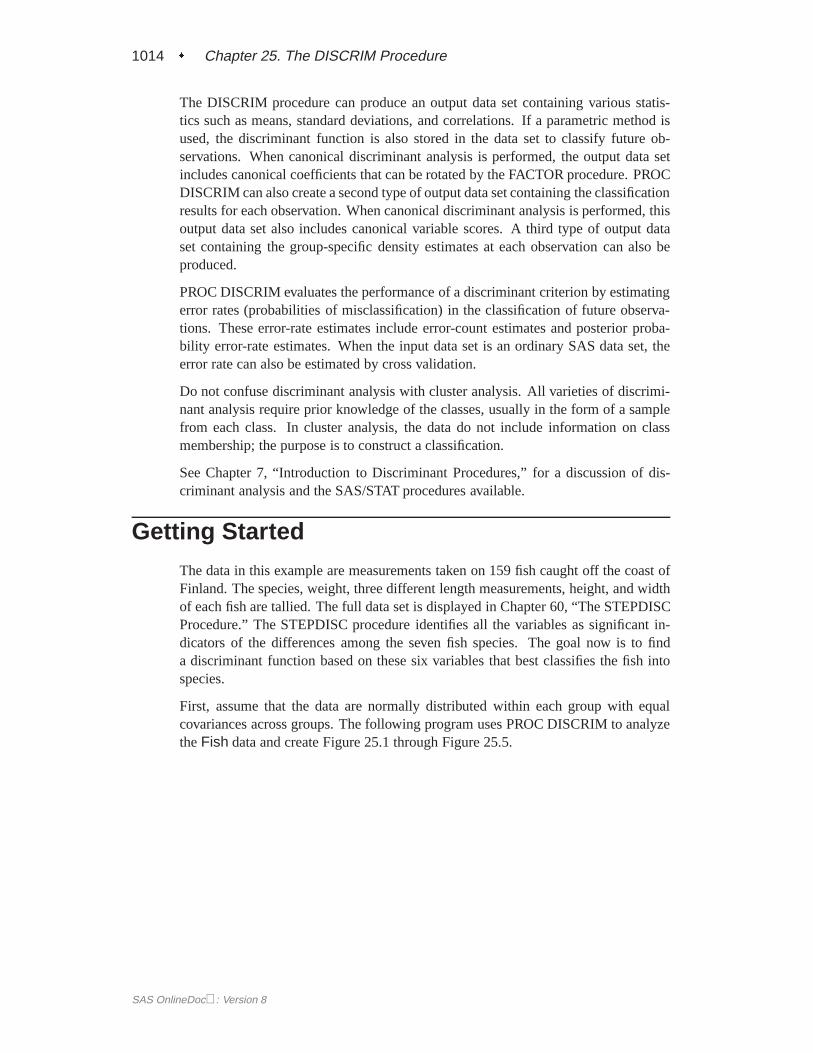
The DISCRIM procedure begins by displaying summary information about the vari-ables in the analysis. This information includes the number of observations, the num-ber of quantitative variables in the analysis (specified with the VAR statement), andthe number of classes in the classification variable (specified with the CLASS state-ment). The frequency of each class, its weight, proportion of the total sample, andprior probability are also displayed. Equal priors are assigned by default.
Fish Measurement Data
The DISCRIM Procedure
Observations 158 DF Total 157Variables 6 DF Within Classes 151Classes 7 DF Between Classes 6
Class Level Information
Variable PriorSpecies Name Frequency Weight Proportion Probability
Bream Bream 34 34.0000 0.215190 0.142857Parkki Parkki 11 11.0000 0.069620 0.142857Perch Perch 56 56.0000 0.354430 0.142857Pike Pike 17 17.0000 0.107595 0.142857Roach Roach 20 20.0000 0.126582 0.142857Smelt Smelt 14 14.0000 0.088608 0.142857Whitefish Whitefish 6 6.0000 0.037975 0.142857
Figure 25.1. Summary Information
SAS OnlineDoc: Version 8
1016 � Chapter 25. The DISCRIM Procedure
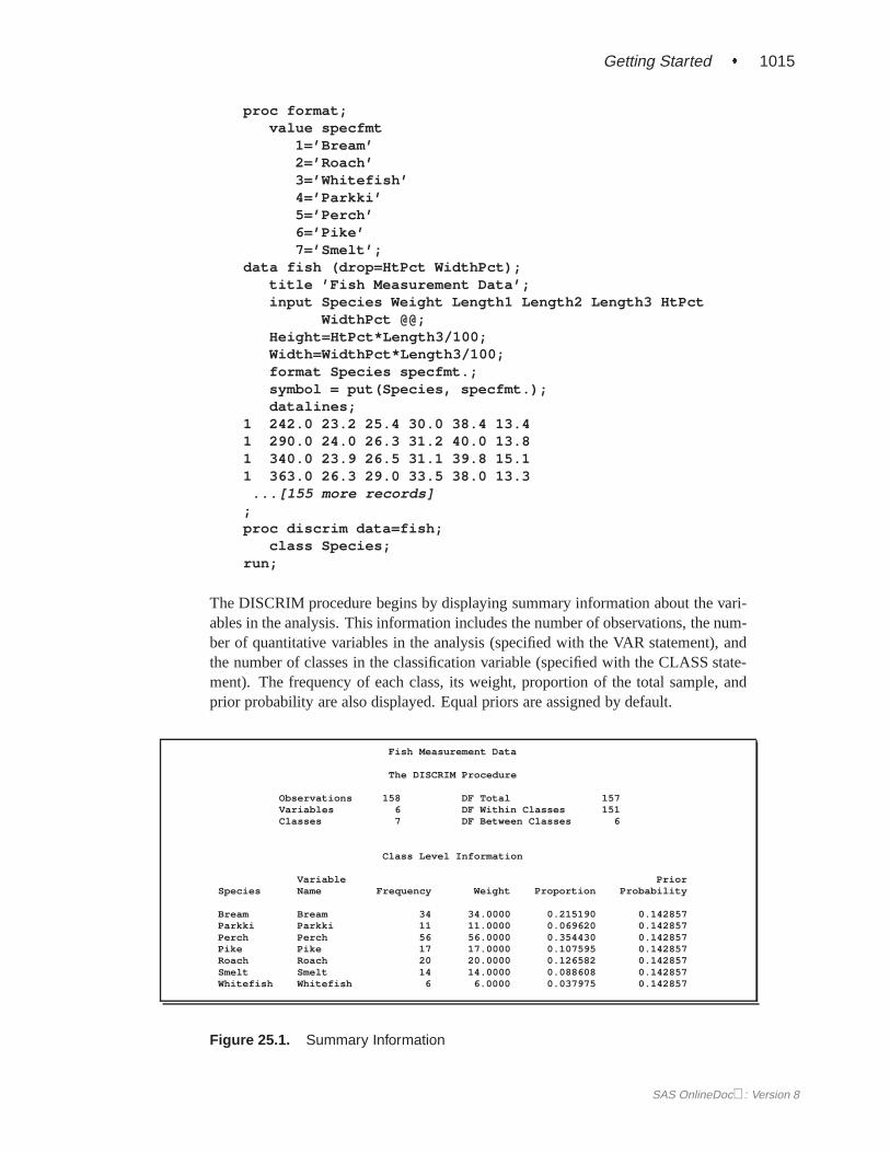
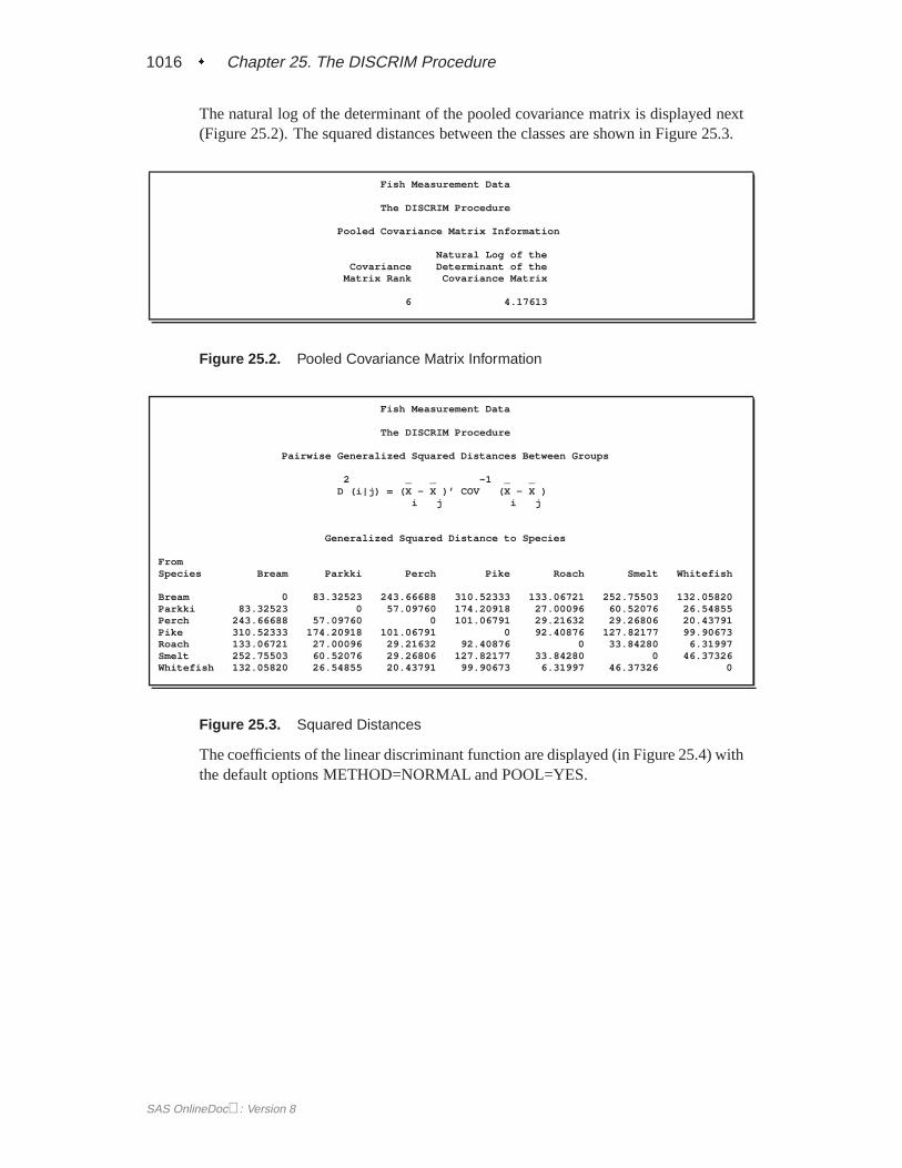
The natural log of the determinant of the pooled covariance matrix is displayed next(Figure 25.2). The squared distances between the classes are shown in Figure 25.3.
Fish Measurement Data
The DISCRIM Procedure
Pooled Covariance Matrix Information
Natural Log of theCovariance Determinant of the
Matrix Rank Covariance Matrix
6 4.17613
Figure 25.2. Pooled Covariance Matrix Information
Fish Measurement Data
The DISCRIM Procedure
Pairwise Generalized Squared Distances Between Groups
2 _ _ -1 _ _D (i|j) = (X - X )’ COV (X - X )
i j i j
Generalized Squared Distance to Species
FromSpecies Bream Parkki Perch Pike Roach Smelt Whitefish
Bream 0 83.32523 243.66688 310.52333 133.06721 252.75503 132.05820Parkki 83.32523 0 57.09760 174.20918 27.00096 60.52076 26.54855Perch 243.66688 57.09760 0 101.06791 29.21632 29.26806 20.43791Pike 310.52333 174.20918 101.06791 0 92.40876 127.82177 99.90673Roach 133.06721 27.00096 29.21632 92.40876 0 33.84280 6.31997Smelt 252.75503 60.52076 29.26806 127.82177 33.84280 0 46.37326Whitefish 132.05820 26.54855 20.43791 99.90673 6.31997 46.37326 0
Figure 25.3. Squared Distances
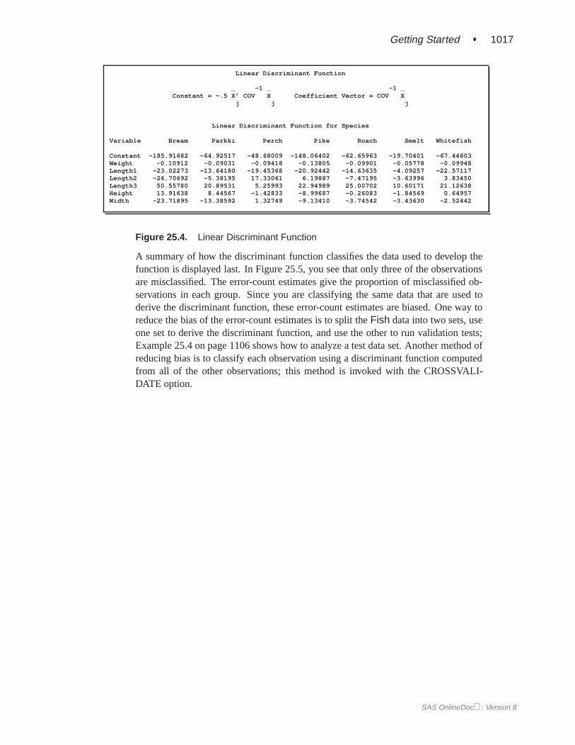
The coefficients of the linear discriminant function are displayed (in Figure 25.4) withthe default options METHOD=NORMAL and POOL=YES.
SAS OnlineDoc: Version 8
Getting Started � 1017
Linear Discriminant Function
_ -1 _ -1 _Constant = -.5 X’ COV X Coefficient Vector = COV X
j j j
Linear Discriminant Function for Species
Variable Bream Parkki Perch Pike Roach Smelt Whitefish
Constant -185.91682 -64.92517 -48.68009 -148.06402 -62.65963 -19.70401 -67.44603Weight -0.10912 -0.09031 -0.09418 -0.13805 -0.09901 -0.05778 -0.09948Length1 -23.02273 -13.64180 -19.45368 -20.92442 -14.63635 -4.09257 -22.57117Length2 -26.70692 -5.38195 17.33061 6.19887 -7.47195 -3.63996 3.83450Length3 50.55780 20.89531 5.25993 22.94989 25.00702 10.60171 21.12638Height 13.91638 8.44567 -1.42833 -8.99687 -0.26083 -1.84569 0.64957Width -23.71895 -13.38592 1.32749 -9.13410 -3.74542 -3.43630 -2.52442
Figure 25.4. Linear Discriminant Function
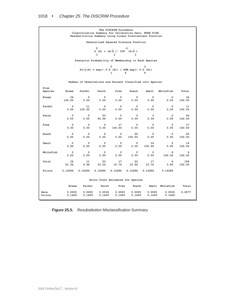
A summary of how the discriminant function classifies the data used to develop thefunction is displayed last. In Figure 25.5, you see that only three of the observationsare misclassified. The error-count estimates give the proportion of misclassified ob-servations in each group. Since you are classifying the same data that are used toderive the discriminant function, these error-count estimates are biased. One way toreduce the bias of the error-count estimates is to split theFish data into two sets, useone set to derive the discriminant function, and use the other to run validation tests;Example 25.4 on page 1106 shows how to analyze a test data set. Another method ofreducing bias is to classify each observation using a discriminant function computedfrom all of the other observations; this method is invoked with the CROSSVALI-DATE option.
SAS OnlineDoc: Version 8
1018 � Chapter 25. The DISCRIM Procedure
The DISCRIM ProcedureClassification Summary for Calibration Data: WORK.FISH
Resubstitution Summary using Linear Discriminant Function
Generalized Squared Distance Function
2 _ -1 _D (X) = (X-X )’ COV (X-X )
j j j
Posterior Probability of Membership in Each Species
2 2Pr(j|X) = exp(-.5 D (X)) / SUM exp(-.5 D (X))
j k k
Number of Observations and Percent Classified into Species
FromSpecies Bream Parkki Perch Pike Roach Smelt Whitefish Total
Bream 34 0 0 0 0 0 0 34100.00 0.00 0.00 0.00 0.00 0.00 0.00 100.00
Parkki 0 11 0 0 0 0 0 110.00 100.00 0.00 0.00 0.00 0.00 0.00 100.00
Perch 0 0 53 0 0 3 0 560.00 0.00 94.64 0.00 0.00 5.36 0.00 100.00
Pike 0 0 0 17 0 0 0 170.00 0.00 0.00 100.00 0.00 0.00 0.00 100.00
Roach 0 0 0 0 20 0 0 200.00 0.00 0.00 0.00 100.00 0.00 0.00 100.00
Smelt 0 0 0 0 0 14 0 140.00 0.00 0.00 0.00 0.00 100.00 0.00 100.00
Whitefish 0 0 0 0 0 0 6 60.00 0.00 0.00 0.00 0.00 0.00 100.00 100.00
Total 34 11 53 17 20 17 6 15821.52 6.96 33.54 10.76 12.66 10.76 3.80 100.00
Priors 0.14286 0.14286 0.14286 0.14286 0.14286 0.14286 0.14286
Error Count Estimates for Species
Bream Parkki Perch Pike Roach Smelt Whitefish Total
Rate 0.0000 0.0000 0.0536 0.0000 0.0000 0.0000 0.0000 0.0077Priors 0.1429 0.1429 0.1429 0.1429 0.1429 0.1429 0.1429
Figure 25.5. Resubstitution Misclassification Summary
SAS OnlineDoc: Version 8
PROC DISCRIM Statement � 1019
Syntax
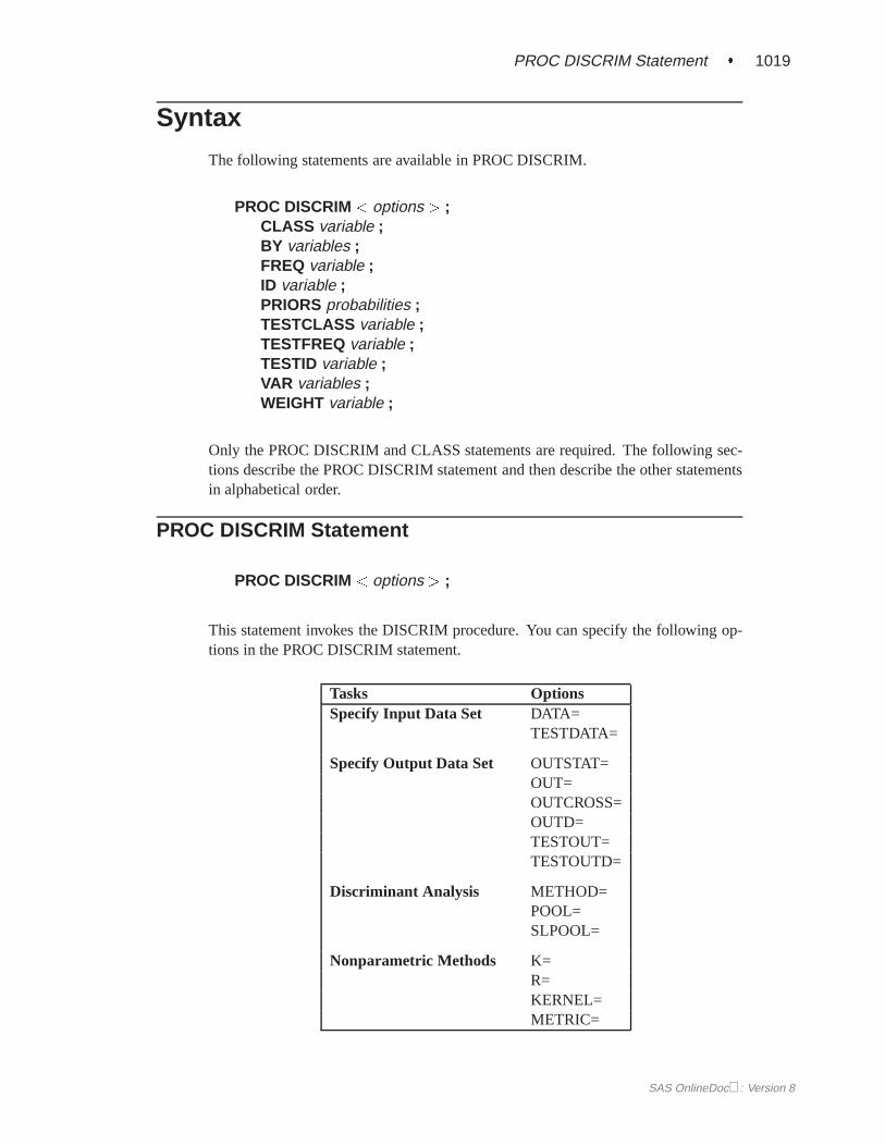
The following statements are available in PROC DISCRIM.
PROC DISCRIM < options > ;CLASS variable ;BY variables ;FREQ variable ;ID variable ;PRIORS probabilities ;TESTCLASS variable ;TESTFREQ variable ;TESTID variable ;VAR variables ;WEIGHT variable ;
Only the PROC DISCRIM and CLASS statements are required. The following sec-tions describe the PROC DISCRIM statement and then describe the other statementsin alphabetical order.
PROC DISCRIM Statement
PROC DISCRIM < options > ;
This statement invokes the DISCRIM procedure. You can specify the following op-tions in the PROC DISCRIM statement.
Tasks OptionsSpecify Input Data Set DATA=
TESTDATA=
Specify Output Data Set OUTSTAT=OUT=OUTCROSS=OUTD=TESTOUT=TESTOUTD=
Discriminant Analysis METHOD=POOL=SLPOOL=
Nonparametric Methods K=R=KERNEL=METRIC=
SAS OnlineDoc: Version 8
1020 � Chapter 25. The DISCRIM Procedure
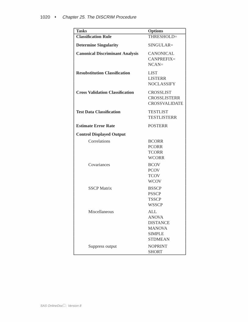
Tasks OptionsClassification Rule THRESHOLD=
Determine Singularity SINGULAR=
Canonical Discriminant Analysis CANONICALCANPREFIX=NCAN=
Resubstitution Classification LISTLISTERRNOCLASSIFY
Cross Validation Classification CROSSLISTCROSSLISTERRCROSSVALIDATE
Test Data Classification TESTLISTTESTLISTERR
Estimate Error Rate POSTERR
Control Displayed Output
Correlations BCORRPCORRTCORRWCORR
Covariances BCOVPCOVTCOVWCOV
SSCP Matrix BSSCPPSSCPTSSCPWSSCP
Miscellaneous ALLANOVADISTANCEMANOVASIMPLESTDMEAN
Suppress output NOPRINTSHORT
SAS OnlineDoc: Version 8
PROC DISCRIM Statement � 1021
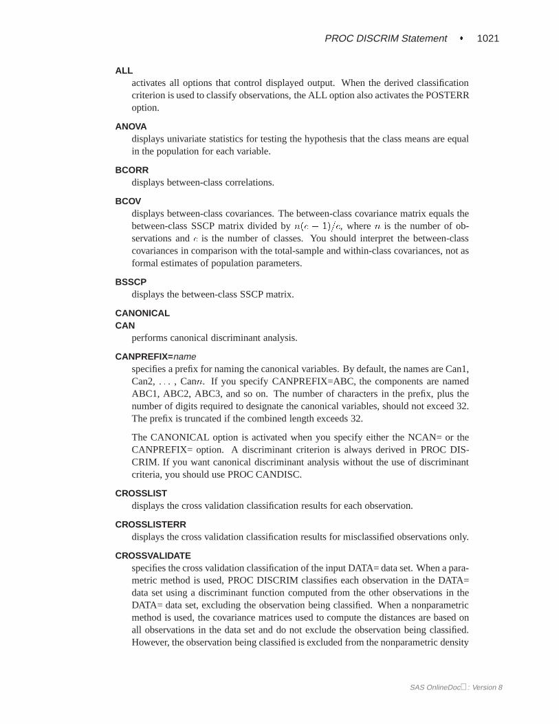
ALLactivates all options that control displayed output. When the derived classificationcriterion is used to classify observations, the ALL option also activates the POSTERRoption.
ANOVAdisplays univariate statistics for testing the hypothesis that the class means are equalin the population for each variable.
BCORRdisplays between-class correlations.
BCOVdisplays between-class covariances. The between-class covariance matrix equals thebetween-class SSCP matrix divided byn(c � 1)=c, wheren is the number of ob-servations andc is the number of classes. You should interpret the between-classcovariances in comparison with the total-sample and within-class covariances, not asformal estimates of population parameters.
BSSCPdisplays the between-class SSCP matrix.
CANONICALCAN
performs canonical discriminant analysis.
CANPREFIX=namespecifies a prefix for naming the canonical variables. By default, the names are Can1,Can2,: : : , Cann. If you specify CANPREFIX=ABC, the components are namedABC1, ABC2, ABC3, and so on. The number of characters in the prefix, plus thenumber of digits required to designate the canonical variables, should not exceed 32.The prefix is truncated if the combined length exceeds 32.
The CANONICAL option is activated when you specify either the NCAN= or theCANPREFIX= option. A discriminant criterion is always derived in PROC DIS-CRIM. If you want canonical discriminant analysis without the use of discriminantcriteria, you should use PROC CANDISC.
CROSSLISTdisplays the cross validation classification results for each observation.
CROSSLISTERRdisplays the cross validation classification results for misclassified observations only.
CROSSVALIDATEspecifies the cross validation classification of the input DATA= data set. When a para-metric method is used, PROC DISCRIM classifies each observation in the DATA=data set using a discriminant function computed from the other observations in theDATA= data set, excluding the observation being classified. When a nonparametricmethod is used, the covariance matrices used to compute the distances are based onall observations in the data set and do not exclude the observation being classified.However, the observation being classified is excluded from the nonparametric density
SAS OnlineDoc: Version 8
1022 � Chapter 25. The DISCRIM Procedure
estimation (if you specify the R= option) or thek nearest neighbors (if you specifythe K= option) of that observation. The CROSSVALIDATE option is set when youspecify the CROSSLIST, CROSSLISTERR, or OUTCROSS= option.
DATA=SAS-data-setspecifies the data set to be analyzed. The data set can be an ordinary SAS data set orone of several specially structured data sets created by SAS/STAT procedures. Thesespecially structured data sets include TYPE=CORR, TYPE=COV, TYPE=CSSCP,TYPE=SSCP, TYPE=LINEAR, TYPE=QUAD, and TYPE=MIXED. The input dataset must be an ordinary SAS data set if you specify METHOD=NPAR. If you omitthe DATA= option, the procedure uses the most recently created SAS data set.
DISTANCE
MAHALANOBIS displays the squared Mahalanobis distances between the groupmeans,F statistics, and the corresponding probabilities of greater Mahalanobissquared distances between the group means. The squared distances are based onthe specification of the POOL= and METRIC= options.
K=kspecifies ak value for thek-nearest-neighbor rule. An observationx is classified intoa group based on the information from thek nearest neighbors ofx. Do not specifyboth the K= and R= options.
KERNEL=BIWEIGHT | BIWKERNEL=EPANECHNIKOV | EPAKERNEL=NORMAL | NORKERNEL=TRIWEIGHT | TRIKERNEL=UNIFORM | UNI
specifies a kernel density to estimate the group-specific densities. You can specifythe KERNEL= option only when the R= option is specified. The default is KER-NEL=UNIFORM.
LISTdisplays the resubstitution classification results for each observation. You can specifythis option only when the input data set is an ordinary SAS data set.
LISTERRdisplays the resubstitution classification results for misclassified observations only.You can specify this option only when the input data set is an ordinary SAS data set.
MANOVAdisplays multivariate statistics for testing the hypothesis that the class means are equalin the population.
METHOD=NORMAL | NPARdetermines the method to use in deriving the classification criterion. When you spec-ify METHOD=NORMAL, a parametric method based on a multivariate normal dis-tribution within each class is used to derive a linear or quadratic discriminant func-tion. The default is METHOD=NORMAL. When you specify METHOD=NPAR, anonparametric method is used and you must also specify either the K= or R= option.
SAS OnlineDoc: Version 8
PROC DISCRIM Statement � 1023
METRIC=DIAGONAL | FULL | IDENTITYspecifies the metric in which the computations of squared distances are performed.If you specify METRIC=FULL, PROC DISCRIM uses either the pooled covariancematrix (POOL=YES) or individual within-group covariance matrices (POOL=NO) tocompute the squared distances. If you specify METRIC=DIAGONAL, PROC DIS-CRIM uses either the diagonal matrix of the pooled covariance matrix (POOL=YES)or diagonal matrices of individual within-group covariance matrices (POOL=NO) tocompute the squared distances. If you specify METRIC=IDENTITY, PROC DIS-CRIM uses Euclidean distance. The default is METRIC=FULL. When you specifyMETHOD=NORMAL, the option METRIC=FULL is used.
NCAN=numberspecifies the number of canonical variables to compute. The value ofnumbermustbe less than or equal to the number of variables. If you specify the option NCAN=0,the procedure displays the canonical correlations but not the canonical coefficients,structures, or means. Letv be the number of variables in the VAR statement andc bethe number of classes. If you omit the NCAN= option, onlymin(v; c � 1) canonicalvariables are generated. If you request an output data set (OUT=, OUTCROSS=,TESTOUT=),v canonical variables are generated. In this case, the lastv � (c � 1)
canonical variables have missing values.
The CANONICAL option is activated when you specify either the NCAN= or theCANPREFIX= option. A discriminant criterion is always derived in PROC DIS-CRIM. If you want canonical discriminant analysis without the use of discriminantcriterion, you should use PROC CANDISC.
NOCLASSIFYsuppresses the resubstitution classification of the input DATA= data set. You canspecify this option only when the input data set is an ordinary SAS data set.
NOPRINTsuppresses the normal display of results. Note that this option temporarily disablesthe Output Delivery System (ODS); see Chapter 15, “Using the Output DeliverySystem,” for more information.
OUT=SAS-data-setcreates an output SAS data set containing all the data from the DATA= data set, plusthe posterior probabilities and the class into which each observation is classified byresubstitution. When you specify the CANONICAL option, the data set also containsnew variables with canonical variable scores. See the “OUT= Data Set” section onpage 1044.
OUTCROSS=SAS-data-setcreates an output SAS data set containing all the data from the DATA= data set,plus the posterior probabilities and the class into which each observation is classifiedby cross validation. When you specify the CANONICAL option, the data set alsocontains new variables with canonical variable scores. See the “OUT= Data Set”section on page 1044.
SAS OnlineDoc: Version 8
1024 � Chapter 25. The DISCRIM Procedure
OUTD=SAS-data-setcreates an output SAS data set containing all the data from the DATA= data set, plusthe group-specific density estimates for each observation. See the “OUT= Data Set”section on page 1044.
OUTSTAT=SAS-data-setcreates an output SAS data set containing various statistics such as means, standarddeviations, and correlations. When the input data set is an ordinary SAS data setor when TYPE=CORR, TYPE=COV, TYPE=CSSCP, or TYPE=SSCP, this optioncan be used to generate discriminant statistics. When you specify the CANONI-CAL option, canonical correlations, canonical structures, canonical coefficients, andmeans of canonical variables for each class are included in the data set. If youspecify METHOD=NORMAL, the output data set also includes coefficients of thediscriminant functions, and the output data set is TYPE=LINEAR (POOL=YES),TYPE=QUAD (POOL=NO), or TYPE=MIXED (POOL=TEST). If you specifyMETHOD=NPAR, this output data set is TYPE=CORR. This data set also holdscalibration information that can be used to classify new observations. See the “Sav-ing and Using Calibration Information” section on page 1041 and the “OUT= DataSet” section on page 1044.
PCORRdisplays pooled within-class correlations.
PCOVdisplays pooled within-class covariances.
POOL=NO | TEST | YESdetermines whether the pooled or within-group covariance matrix is the basis of themeasure of the squared distance. If you specify POOL=YES, PROC DISCRIM usesthe pooled covariance matrix in calculating the (generalized) squared distances. Lin-ear discriminant functions are computed. If you specify POOL=NO, the procedureuses the individual within-group covariance matrices in calculating the distances.Quadratic discriminant functions are computed. The default is POOL=YES.
When you specify METHOD=NORMAL, the option POOL=TEST requestsBartlett’s modification of the likelihood ratio test (Morrison 1976; Anderson 1984)of the homogeneity of the within-group covariance matrices. The test is unbiased(Perlman 1980). However, it is not robust to nonnormality. If the test statistic is sig-nificant at the level specified by the SLPOOL= option, the within-group covariancematrices are used. Otherwise, the pooled covariance matrix is used. The discriminantfunction coefficients are displayed only when the pooled covariance matrix is used.
POSTERRdisplays the posterior probability error-rate estimates of the classification criterionbased on the classification results.
PSSCPdisplays the pooled within-class corrected SSCP matrix.
SAS OnlineDoc: Version 8
PROC DISCRIM Statement � 1025
R=rspecifies a radiusr value for kernel density estimation. With uniform, Epanechnikov,biweight, or triweight kernels, an observationx is classified into a group based onthe information from observationsy in the training set within the radiusr of x, thatis, the groupt observationsy with squared distanced2t (x;y) � r2. When a normalkernel is used, the classification of an observationx is based on the information ofthe estimated group-specific densities from all observations in the training set. Thematrix r2Vt is used as the groupt covariance matrix in the normal-kernel density,whereVt is the matrix used in calculating the squared distances. Do not specify boththe K= and R= options. For more information on selectingr, see the “NonparametricMethods” section on page 1033.
SHORTsuppresses the display of certain items in the default output. If you specifyMETHOD= NORMAL, PROC DISCRIM suppresses the display of determinants,generalized squared distances between-class means, and discriminant function coef-ficients. When you specify the CANONICAL option, PROC DISCRIM suppressesthe display of canonical structures, canonical coefficients, and class means on canon-ical variables; only tables of canonical correlations are displayed.
SIMPLEdisplays simple descriptive statistics for the total sample and within each class.
SINGULAR=pspecifies the criterion for determining the singularity of a matrix, where0 < p < 1.The default is SINGULAR=1E�8.
Let S be the total-sample correlation matrix. If theR2 for predicting a quantitativevariable in the VAR statement from the variables preceding it exceeds1 � p, thenSis considered singular. IfS is singular, the probability levels for the multivariate teststatistics and canonical correlations are adjusted for the number of variables withR2
exceeding1� p.
Let St be the groupt covariance matrix andSp be the pooled covariance matrix. Ingroup t, if the R2 for predicting a quantitative variable in the VAR statement fromthe variables preceding it exceeds1 � p, thenSt is considered singular. Similarly,if the partialR2 for predicting a quantitative variable in the VAR statement from thevariables preceding it, after controlling for the effect of the CLASS variable, exceeds1� p, thenSp is considered singular.
If PROC DISCRIM needs to compute either the inverse or the determinant of a matrixthat is considered singular, then it uses a quasi-inverse or a quasi-determinant. Fordetails, see the “Quasi-Inverse” section on page 1038.
SLPOOL=pspecifies the significance level for the test of homogeneity. You can specify theSLPOOL= option only when POOL=TEST is also specified. If you specify POOL=TEST but omit the SLPOOL= option, PROC DISCRIM uses 0.10 as the significancelevel for the test.
SAS OnlineDoc: Version 8
1026 � Chapter 25. The DISCRIM Procedure
STDMEANdisplays total-sample and pooled within-class standardized class means.
TCORRdisplays total-sample correlations.
TCOVdisplays total-sample covariances.
TESTDATA=SAS-data-setnames an ordinary SAS data set with observations that are to be classified. Thequantitative variable names in this data set must match those in the DATA= data set.When you specify the TESTDATA= option, you can also specify the TESTCLASS,TESTFREQ, and TESTID statements. When you specify the TESTDATA= option,you can use the TESTOUT= and TESTOUTD= options to generate classificationresults and group-specific density estimates for observations in the test data set.
TESTLISTlists classification results for all observations in the TESTDATA= data set.
TESTLISTERRlists only misclassified observations in the TESTDATA= data set but only if a TEST-CLASS statement is also used.
TESTOUT=SAS-data-setcreates an output SAS data set containing all the data from the TESTDATA= data set,plus the posterior probabilities and the class into which each observation is classified.When you specify the CANONICAL option, the data set also contains new variableswith canonical variable scores. See the “OUT= Data Set” section on page 1044.
TESTOUTD=SAS-data-setcreates an output SAS data set containing all the data from the TESTDATA= data set,plus the group-specific density estimates for each observation. See the “OUT= DataSet” section on page 1044.
THRESHOLD=pspecifies the minimum acceptable posterior probability for classification, where0 �p � 1. If the largest posterior probability of group membership is less than theTHRESHOLD value, the observation is classified into group OTHER. The default isTHRESHOLD=0.
TSSCPdisplays the total-sample corrected SSCP matrix.
WCORRdisplays within-class correlations for each class level.
WCOVdisplays within-class covariances for each class level.
WSSCPdisplays the within-class corrected SSCP matrix for each class level.
SAS OnlineDoc: Version 8
BY Statement � 1027
BY Statement
BY variables ;
You can specify a BY statement with PROC DISCRIM to obtain separate analyses onobservations in groups defined by the BY variables. When a BY statement appears,the procedure expects the input data set to be sorted in order of the BY variables.
If your input data set is not sorted in ascending order, use one of the following alter-natives:
� Sort the data using the SORT procedure with a similar BY statement.
� Specify the BY statement option NOTSORTED or DESCENDING in the BYstatement for the DISCRIM procedure. The NOTSORTED option does notmean that the data are unsorted but rather that the data are arranged in groups(according to values of the BY variables) and that these groups are not neces-sarily in alphabetical or increasing numeric order.
� Create an index on the BY variables using the DATASETS procedure (in baseSAS software).
For more information on the BY statement, refer toSAS Language Reference: Con-cepts. For more information on the DATASETS procedure, see the discussion in theSAS Procedures Guide.
If you specify the TESTDATA= option and the TESTDATA= data set does not containany of the BY variables, then the entire TESTDATA= data set is classified accordingto the discriminant functions computed in each BY group in the DATA= data set.
If the TESTDATA= data set contains some but not all of the BY variables, or if someBY variables do not have the same type or length in the TESTDATA= data set as inthe DATA= data set, then PROC DISCRIM displays an error message and stops.
If all BY variables appear in the TESTDATA= data set with the same type and lengthas in the DATA= data set, then each BY group in the TESTDATA= data set is clas-sified by the discriminant function from the corresponding BY group in the DATA=data set. The BY groups in the TESTDATA= data set must be in the same order asin the DATA= data set. If you specify the NOTSORTED option in the BY statement,there must be exactly the same BY groups in the same order in both data sets. Ifyou omit the NOTSORTED option, some BY groups may appear in one data set butnot in the other. If some BY groups appear in the TESTDATA= data set but not inthe DATA= data set, and you request an output test data set using the TESTOUT= orTESTOUTD= option, these BY groups are not included in the output data set.
SAS OnlineDoc: Version 8
1028 � Chapter 25. The DISCRIM Procedure
CLASS Statement
CLASS variable ;
The values of the classification variable define the groups for analysis. Class levelsare determined by the formatted values of the CLASS variable. The specified variablecan be numeric or character. A CLASS statement is required.
FREQ Statement
FREQ variable ;
If a variable in the data set represents the frequency of occurrence for the other valuesin the observation, include the variable’s name in a FREQ statement. The procedurethen treats the data set as if each observation appearsn times, wheren is the valueof the FREQ variable for the observation. The total number of observations is con-sidered to be equal to the sum of the FREQ variable when the procedure determinesdegrees of freedom for significance probabilities.
If the value of the FREQ variable is missing or is less than one, the observation is notused in the analysis. If the value is not an integer, it is truncated to an integer.
ID Statement
ID variable ;
The ID statement is effective only when you specify the LIST or LISTERR option inthe PROC DISCRIM statement. When the DISCRIM procedure displays the classi-fication results, the ID variable (rather than the observation number) is displayed foreach observation.
PRIORS Statement
PRIORS EQUAL;
PRIORS PROPORTIONAL | PROP;
PRIORS probabilities ;
The PRIORS statement specifies the prior probabilities of group membership. To setthe prior probabilities equal, use
priors equal;
To set the prior probabilities proportional to the sample sizes, use
priors proportional;
SAS OnlineDoc: Version 8
TESTCLASS Statement � 1029
For other than equal or proportional priors, specify the prior probability for each levelof the classification variable. Each class level can be written as either a SAS nameor a quoted string, and it must be followed by an equal sign and a numeric constantbetween zero and one. A SAS name begins with a letter or an underscore and cancontain digits as well. Lowercase character values and data values with leading blanksmust be enclosed in quotes. For example, to define prior probabilities for each levelof Grade, whereGrade’s values are A, B, C, and D, the PRIORS statement can be
priors A=0.1 B=0.3 C=0.5 D=0.1;
If Grade’s values are ’a’, ’b’, ’c’, and ’d’, each class level must be written as a quotedstring:
priors ’a’=0.1 ’b’=0.3 ’c’=0.5 ’d’=0.1;
If Grade is numeric, with formatted values of ’1’, ’2’, and ’3’, the PRIORS statementcan be
priors ’1’=0.3 ’2’=0.6 ’3’=0.1;
The specified class levels must exactly match the formatted values of the CLASSvariable. For example, if a CLASS variableC has the format 4.2 and a value 5, thePRIORS statement must specify ’5.00’, not ’5.0’ or ’5’. If the prior probabilities donot sum to one, these probabilities are scaled proportionally to have the sum equal toone. The default is PRIORS EQUAL.
TESTCLASS Statement
TESTCLASS variable ;
The TESTCLASS statement names the variable in the TESTDATA= data set that isused to determine whether an observation in the TESTDATA= data set is misclassi-fied. The TESTCLASS variable should have the same type (character or numeric)and length as the variable given in the CLASS statement. PROC DISCRIM con-siders an observation misclassified when the formatted value of the TESTCLASSvariable does not match the group into which the TESTDATA= observation is clas-sified. When the TESTCLASS statement is missing and the TESTDATA= data setcontains the variable given in the CLASS statement, the CLASS variable is used asthe TESTCLASS variable.
SAS OnlineDoc: Version 8
1030 � Chapter 25. The DISCRIM Procedure
TESTFREQ Statement
TESTFREQ variable ;
If a variable in the TESTDATA= data set represents the frequency of occurrence forthe other values in the observation, include the variable’s name in a TESTFREQstatement. The procedure then treats the data set as if each observation appearsntimes, wheren is the value of the TESTFREQ variable for the observation.
If the value of the TESTFREQ variable is missing or is less than one, the observationis not used in the analysis. If the value is not an integer, it is truncated to an integer.
TESTID Statement
TESTID variable ;
The TESTID statement is effective only when you specify the TESTLIST orTESTLISTERR option in the PROC DISCRIM statement. When the DISCRIM pro-cedure displays the classification results for the TESTDATA= data set, the TESTIDvariable (rather than the observation number) is displayed for each observation. Thevariable given in the TESTID statement must be in the TESTDATA= data set.
VAR Statement
VAR variables ;
The VAR statement specifies the quantitative variables to be included in the analysis.The default is all numeric variables not listed in other statements.
WEIGHT Statement
WEIGHT variable ;
To use relative weights for each observation in the input data set, place the weights ina variable in the data set and specify the name in a WEIGHT statement. This is oftendone when the variance associated with each observation is different and the valuesof the weight variable are proportional to the reciprocals of the variances. If the valueof the WEIGHT variable is missing or is less than zero, then a value of zero for theweight is used.
SAS OnlineDoc: Version 8
Background � 1031
The WEIGHT and FREQ statements have a similar effect except that the WEIGHTstatement does not alter the degrees of freedom.
Details
Missing Values
Observations with missing values for variables in the analysis are excluded from thedevelopment of the classification criterion. When the values of the classification vari-able are missing, the observation is excluded from the development of the classifi-cation criterion, but if no other variables in the analysis have missing values for thatobservation, the observation is classified and displayed with the classification results.
Background
The following notation is used to describe the classification methods:
x ap-dimensional vector containing the quantitative variables of an observation
Sp the pooled covariance matrix
t a subscript to distinguish the groups
nt the number of training set observations in groupt
mt thep-dimensional vector containing variable means in groupt
St the covariance matrix within groupt
jStj the determinant ofSt
qt the prior probability of membership in groupt
p(tjx) the posterior probability of an observationx belonging to groupt
ft the probability density function for groupt
ft(x) the group-specific density estimate atx from groupt
f(x)P
t qtft(x), the estimated unconditional density atx
et the classification error rate for groupt
Bayes’ TheoremAssuming that the prior probabilities of group membership are known and that thegroup-specific densities atx can be estimated, PROC DISCRIM computesp(tjx),the probability ofx belonging to groupt, by applying Bayes’ theorem:
p(tjx) =qtft(x)
f(x)
PROC DISCRIM partitions ap-dimensional vector space into regionsRt, where theregionRt is the subspace containing allp-dimensional vectorsy such thatp(tjy) is
SAS OnlineDoc: Version 8
1032 � Chapter 25. The DISCRIM Procedure
the largest among all groups. An observation is classified as coming from groupt ifit lies in regionRt.
Parametric MethodsAssuming that each group has a multivariate normal distribution, PROC DISCRIMdevelops a discriminant function or classification criterion using a measure of gener-alized squared distance. The classification criterion is based on either the individualwithin-group covariance matrices or the pooled covariance matrix; it also takes intoaccount the prior probabilities of the classes. Each observation is placed in the classfrom which it has the smallest generalized squared distance. PROC DISCRIM alsocomputes the posterior probability of an observation belonging to each class.
The squared Mahalanobis distance fromx to groupt is
d2t (x) = (x�mt)0V�1
t (x�mt)
whereVt = St if the within-group covariance matrices are used, orVt = Sp if thepooled covariance matrix is used.
The group-specific density estimate atx from group t is then given by
ft(x) = (2�)�p
2 jVtj�1
2 exp��0:5d2t (x)
�Using Bayes’ theorem, the posterior probability ofx belonging to groupt is
p(tjx) =qtft(x)Pu qufu(x)
where the summation is over all groups.
The generalized squared distance fromx to groupt is defined as
D2t (x) = d2t (x) + g1(t) + g2(t)
where
g1(t) =
�ln jStj if the within-group covariance matrices are used0 if the pooled covariance matrix is used
and
g2(t) =
��2 ln(qt) if the prior probabilities are not all equal0 if the prior probabilities are all equal
The posterior probability ofx belonging to groupt is then equal to
p(tjx) =exp
��0:5D2
t (x)�P
u exp (�0:5D2u(x))
SAS OnlineDoc: Version 8
Background � 1033
The discriminant scores are�0:5D2u(x). An observation is classified into groupu
if setting t = u produces the largest value ofp(tjx) or the smallest value ofD2t (x).
If this largest posterior probability is less than the threshold specified,x is classifiedinto group OTHER.
Nonparametric MethodsNonparametric discriminant methods are based on nonparametric estimates of group-specific probability densities. Either a kernel method or thek-nearest-neighbormethod can be used to generate a nonparametric density estimate in each group and toproduce a classification criterion. The kernel method uses uniform, normal, Epanech-nikov, biweight, or triweight kernels in the density estimation.
Either Mahalanobis distance or Euclidean distance can be used to determine prox-imity. When thek-nearest-neighbor method is used, the Mahalanobis distances arebased on the pooled covariance matrix. When a kernel method is used, the Maha-lanobis distances are based on either the individual within-group covariance matricesor the pooled covariance matrix. Either the full covariance matrix or the diagonalmatrix of variances can be used to calculate the Mahalanobis distances.
The squared distance between two observation vectors,x andy, in groupt is givenby
d2t (x;y) = (x� y)0V �1t (x� y)
whereVt has one of the following forms:
Vt =
8>>>><>>>>:
Sp the pooled covariance matrixdiag(Sp) the diagonal matrix of the pooled covariance matrixSt the covariance matrix within grouptdiag(St) the diagonal matrix of the covariance matrix within grouptI the identity matrix
The classification of an observation vectorx is based on the estimated group-specificdensities from the training set. From these estimated densities, the posterior proba-bilities of group membership atx are evaluated. An observationx is classified intogroupu if setting t = u produces the largest value ofp(tjx). If there is a tie for thelargest probability or if this largest probability is less than the threshold specified,x
is classified into group OTHER.
The kernel method uses a fixed radius,r, and a specified kernel,Kt, to estimate thegroupt density at each observation vectorx. Let z be ap-dimensional vector. Thenthe volume of ap-dimensional unit sphere bounded byz0z = 1 is
v0 =�
p
2
��p2+ 1�
where� represents the gamma function (refer toSAS Language Reference: Dictio-nary).
SAS OnlineDoc: Version 8
1034 � Chapter 25. The DISCRIM Procedure
Thus, in groupt, the volume of ap-dimensional ellipsoid bounded byfz j z0V�1
t z = r2g is
vr(t) = rpjVtj1
2 v0
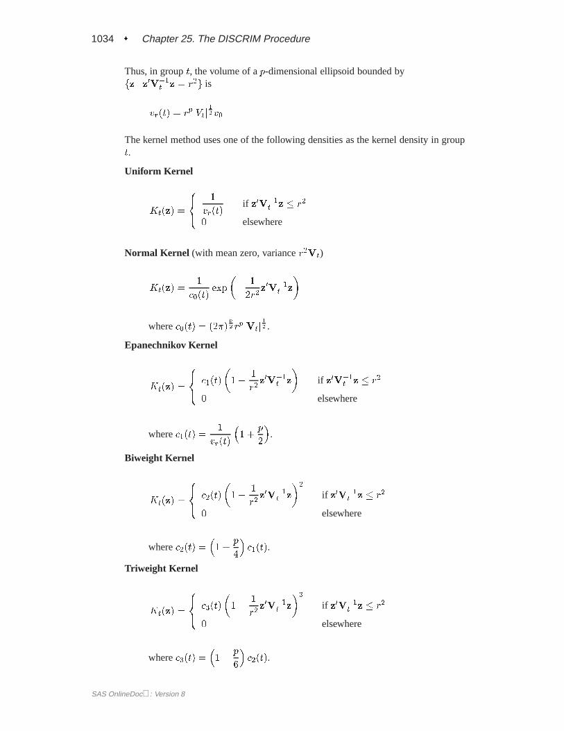
The kernel method uses one of the following densities as the kernel density in groupt.
Uniform Kernel
Kt(z) =
8<:
1
vr(t)if z0V�1
t z � r2
0 elsewhere
Normal Kernel (with mean zero, variancer2Vt)
Kt(z) =1
c0(t)exp
��
1
2r2z0V�1
t z
�
wherec0(t) = (2�)p
2 rpjVtj1
2 .
Epanechnikov Kernel
Kt(z) =
8<: c1(t)
�1�
1
r2z0V�1
t z
�if z0V�1
t z � r2
0 elsewhere
wherec1(t) =1
vr(t)
�1 +
p
2
�.
Biweight Kernel
Kt(z) =
8<: c2(t)
�1�
1
r2z0V�1
t z
�2if z0V�1
t z � r2
0 elsewhere
wherec2(t) =�1 +
p
4
�c1(t).
Triweight Kernel
Kt(z) =
8<: c3(t)
�1�
1
r2z0V�1
t z
�3if z0V�1
t z � r2
0 elsewhere
wherec3(t) =�1 +
p
6
�c2(t).
SAS OnlineDoc: Version 8
Background � 1035
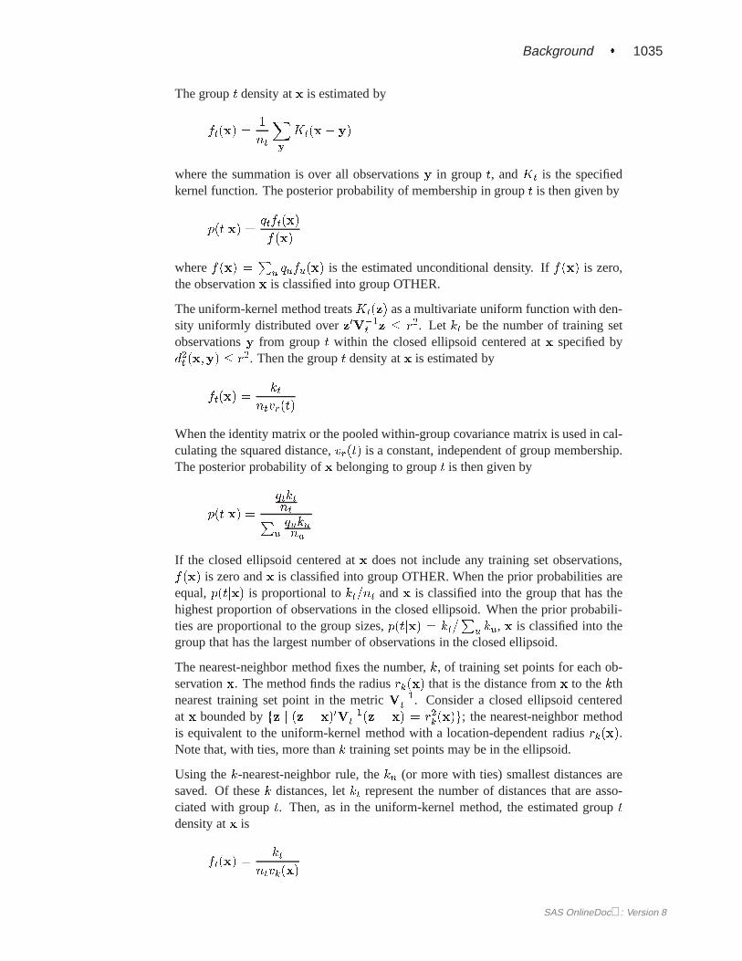
The groupt density atx is estimated by
ft(x) =1
nt
Xy
Kt(x� y)
where the summation is over all observationsy in group t, andKt is the specifiedkernel function. The posterior probability of membership in groupt is then given by
p(tjx) =qtft(x)
f(x)
wheref(x) =P
u qufu(x) is the estimated unconditional density. Iff(x) is zero,the observationx is classified into group OTHER.
The uniform-kernel method treatsKt(z) as a multivariate uniform function with den-sity uniformly distributed overz0V�1
t z � r2. Let kt be the number of training setobservationsy from groupt within the closed ellipsoid centered atx specified byd2t (x;y) � r2. Then the groupt density atx is estimated by
ft(x) =kt
ntvr(t)
When the identity matrix or the pooled within-group covariance matrix is used in cal-culating the squared distance,vr(t) is a constant, independent of group membership.The posterior probability ofx belonging to groupt is then given by
p(tjx) =
qtktntP
uqukunu
If the closed ellipsoid centered atx does not include any training set observations,f(x) is zero andx is classified into group OTHER. When the prior probabilities areequal,p(tjx) is proportional tokt=nt andx is classified into the group that has thehighest proportion of observations in the closed ellipsoid. When the prior probabili-ties are proportional to the group sizes,p(tjx) = kt=
Pu ku, x is classified into the
group that has the largest number of observations in the closed ellipsoid.
The nearest-neighbor method fixes the number,k, of training set points for each ob-servationx. The method finds the radiusrk(x) that is the distance fromx to thekthnearest training set point in the metricV�1
t . Consider a closed ellipsoid centeredat x bounded byfz j (z � x)0V�1
t (z � x) = r2k(x)g; the nearest-neighbor methodis equivalent to the uniform-kernel method with a location-dependent radiusrk(x).Note that, with ties, more thank training set points may be in the ellipsoid.
Using thek-nearest-neighbor rule, thekn (or more with ties) smallest distances aresaved. Of thesek distances, letkt represent the number of distances that are asso-ciated with groupt. Then, as in the uniform-kernel method, the estimated grouptdensity atx is
ft(x) =kt
ntvk(x)
SAS OnlineDoc: Version 8
1036 � Chapter 25. The DISCRIM Procedure
wherevk(x) is the volume of the ellipsoid bounded byfz j (z � x)0V�1t (z � x) =
r2k(x)g. Since the pooled within-group covariance matrix is used to calculate thedistances used in the nearest-neighbor method, the volumevk(x) is a constant inde-pendent of group membership. Whenk = 1 is used in the nearest-neighbor rule,x isclassified into the group associated with they point that yields the smallest squareddistanced2t (x;y). Prior probabilities affect nearest-neighbor results in the same waythat they affect uniform-kernel results.
With a specified squared distance formula (METRIC=, POOL=), the values ofr andk determine the degree of irregularity in the estimate of the density function, andthey are called smoothing parameters. Small values ofr or k produce jagged densityestimates, and large values ofr or k produce smoother density estimates. Variousmethods for choosing the smoothing parameters have been suggested, and there is asyet no simple solution to this problem.
For a fixed kernel shape, one way to choose the smoothing parameterr is to plotestimated densities with different values ofr and to choose the estimate that is mostin accordance with the prior information about the density. For many applications,this approach is satisfactory.
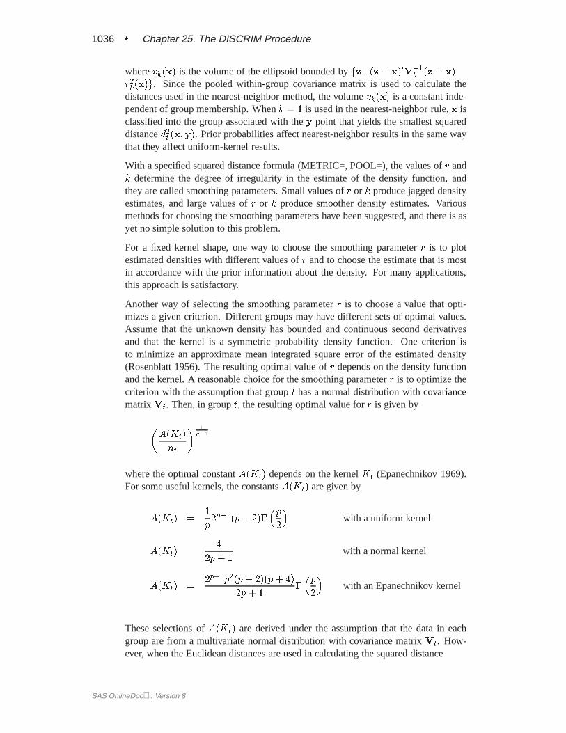
Another way of selecting the smoothing parameterr is to choose a value that opti-mizes a given criterion. Different groups may have different sets of optimal values.Assume that the unknown density has bounded and continuous second derivativesand that the kernel is a symmetric probability density function. One criterion isto minimize an approximate mean integrated square error of the estimated density(Rosenblatt 1956). The resulting optimal value ofr depends on the density functionand the kernel. A reasonable choice for the smoothing parameterr is to optimize thecriterion with the assumption that groupt has a normal distribution with covariancematrixVt. Then, in groupt, the resulting optimal value forr is given by
�A(Kt)
nt
� 1
p+4
where the optimal constantA(Kt) depends on the kernelKt (Epanechnikov 1969).For some useful kernels, the constantsA(Kt) are given by
A(Kt) =1
p2p+1(p+ 2)�
�p2
�with a uniform kernel
A(Kt) =4
2p+ 1with a normal kernel
A(Kt) =2p+2p2(p+ 2)(p + 4)
2p+ 1��p2
�with an Epanechnikov kernel
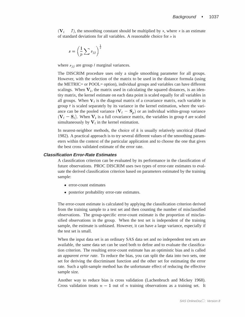
These selections ofA(Kt) are derived under the assumption that the data in eachgroup are from a multivariate normal distribution with covariance matrixVt. How-ever, when the Euclidean distances are used in calculating the squared distance
SAS OnlineDoc: Version 8
Background � 1037
(Vt = I), the smoothing constant should be multiplied bys, wheres is an estimateof standard deviations for all variables. A reasonable choice fors is
s =
�1
p
Xsjj
� 1
2
wheresjj are groupt marginal variances.
The DISCRIM procedure uses only a single smoothing parameter for all groups.However, with the selection of the matrix to be used in the distance formula (usingthe METRIC= or POOL= option), individual groups and variables can have differentscalings. WhenVt, the matrix used in calculating the squared distances, is an iden-tity matrix, the kernel estimate on each data point is scaled equally for all variables inall groups. WhenVt is the diagonal matrix of a covariance matrix, each variable ingroupt is scaled separately by its variance in the kernel estimation, where the vari-ance can be the pooled variance(Vt = Sp) or an individual within-group variance(Vt = St). WhenVt is a full covariance matrix, the variables in groupt are scaledsimultaneously byVt in the kernel estimation.
In nearest-neighbor methods, the choice ofk is usually relatively uncritical (Hand1982). A practical approach is to try several different values of the smoothing param-eters within the context of the particular application and to choose the one that givesthe best cross validated estimate of the error rate.
Classification Error-Rate EstimatesA classification criterion can be evaluated by its performance in the classification offuture observations. PROC DISCRIM uses two types of error-rate estimates to eval-uate the derived classification criterion based on parameters estimated by the trainingsample:
� error-count estimates
� posterior probability error-rate estimates.
The error-count estimate is calculated by applying the classification criterion derivedfrom the training sample to a test set and then counting the number of misclassifiedobservations. The group-specific error-count estimate is the proportion of misclas-sified observations in the group. When the test set is independent of the trainingsample, the estimate is unbiased. However, it can have a large variance, especially ifthe test set is small.
When the input data set is an ordinary SAS data set and no independent test sets areavailable, the same data set can be used both to define and to evaluate the classifica-tion criterion. The resulting error-count estimate has an optimistic bias and is calledanapparent error rate. To reduce the bias, you can split the data into two sets, oneset for deriving the discriminant function and the other set for estimating the errorrate. Such a split-sample method has the unfortunate effect of reducing the effectivesample size.
Another way to reduce bias is cross validation (Lachenbruch and Mickey 1968).Cross validation treatsn � 1 out of n training observations as a training set. It
SAS OnlineDoc: Version 8
1038 � Chapter 25. The DISCRIM Procedure
determines the discriminant functions based on thesen � 1 observations and thenapplies them to classify the one observation left out. This is done for each of then training observations. The misclassification rate for each group is the proportionof sample observations in that group that are misclassified. This method achieves anearly unbiased estimate but with a relatively large variance.
To reduce the variance in an error-count estimate, smoothed error-rate estimates aresuggested (Glick 1978). Instead of summing terms that are either zero or one asin the error-count estimator, the smoothed estimator uses a continuum of values be-tween zero and one in the terms that are summed. The resulting estimator has asmaller variance than the error-count estimate. The posterior probability error-rateestimates provided by the POSTERR option in the PROC DISCRIM statement (seethe following section, “Posterior Probability Error-Rate Estimates”) are smoothederror-rate estimates. The posterior probability estimates for each group are based onthe posterior probabilities of the observations classified into that same group. Theposterior probability estimates provide good estimates of the error rate when the pos-terior probabilities are accurate. When a parametric classification criterion (linear orquadratic discriminant function) is derived from a nonnormal population, the result-ing posterior probability error-rate estimators may not be appropriate.
The overall error rate is estimated through a weighted average of the individual group-specific error-rate estimates, where the prior probabilities are used as the weights.
To reduce both the bias and the variance of the estimator, Hora and Wilcox (1982)compute the posterior probability estimates based on cross validation. The resultingestimates are intended to have both low variance from using the posterior probabil-ity estimate and low bias from cross validation. They use Monte Carlo studies ontwo-group multivariate normal distributions to compare the cross validation posteriorprobability estimates with three other estimators: the apparent error rate, cross val-idation estimator, and posterior probability estimator. They conclude that the crossvalidation posterior probability estimator has a lower mean squared error in their sim-ulations.
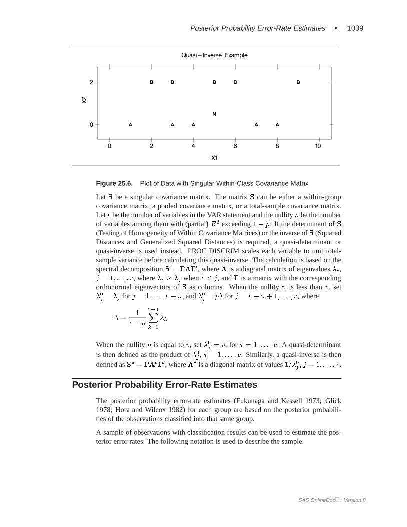
Quasi-InverseConsider the plot shown in Figure 25.6 with two variables,X1 and X2, and twoclasses, A and B. The within-class covariance matrix is diagonal, with a positive valuefor X1 but zero forX2. Using a Moore-Penrose pseudo-inverse would effectively ig-noreX2 completely in doing the classification, and the two classes would have a zerogeneralized distance and could not be discriminated at all. The quasi-inverse usedby PROC DISCRIM replaces the zero variance forX2 by a small positive number toremove the singularity. This allowsX2 to be used in the discrimination and resultscorrectly in a large generalized distance between the two classes and a zero errorrate. It also allows new observations, such as the one indicated by N, to be classifiedin a reasonable way. PROC CANDISC also uses a quasi-inverse when the total-sample covariance matrix is considered to be singular and Mahalanobis distances arerequested. This problem with singular within-class covariance matrices is discussedin Ripley (1996, p. 38). The use of the quasi-inverse is an innovation introduced bySAS Institute Inc.
SAS OnlineDoc: Version 8
Posterior Probability Error-Rate Estimates � 1039
Figure 25.6. Plot of Data with Singular Within-Class Covariance Matrix
Let S be a singular covariance matrix. The matrixS can be either a within-groupcovariance matrix, a pooled covariance matrix, or a total-sample covariance matrix.Letv be the number of variables in the VAR statement and the nullityn be the numberof variables among them with (partial)R2 exceeding1 � p. If the determinant ofS(Testing of Homogeneity of Within Covariance Matrices) or the inverse ofS (SquaredDistances and Generalized Squared Distances) is required, a quasi-determinant orquasi-inverse is used instead. PROC DISCRIM scales each variable to unit total-sample variance before calculating this quasi-inverse. The calculation is based on thespectral decompositionS = ���0, where� is a diagonal matrix of eigenvalues�j,j = 1; : : : ; v, where�i � �j wheni < j, and� is a matrix with the correspondingorthonormal eigenvectors ofS as columns. When the nullityn is less thanv, set�0j = �j for j = 1; : : : ; v � n, and�0j = p�� for j = v � n+ 1; : : : ; v, where
�� =1
v � n
v�nXk=1
�k
When the nullityn is equal tov, set�0j = p, for j = 1; : : : ; v. A quasi-determinantis then defined as the product of�0j , j = 1; : : : ; v. Similarly, a quasi-inverse is thendefined asS� = ����0, where�� is a diagonal matrix of values1=�0j ; j = 1; : : : ; v.
Posterior Probability Error-Rate Estimates
The posterior probability error-rate estimates (Fukunaga and Kessell 1973; Glick1978; Hora and Wilcox 1982) for each group are based on the posterior probabili-ties of the observations classified into that same group.
A sample of observations with classification results can be used to estimate the pos-terior error rates. The following notation is used to describe the sample.
SAS OnlineDoc: Version 8
1040 � Chapter 25. The DISCRIM Procedure
S the set of observations in the (training) sample
n the number of observations inS
nt the number of observations inS in groupt
Rt the set of observations such that the posterior probability belonging to groupt is the largest
Rut the set of observations from groupu such that the posterior probability be-longing to groupt is the largest.
The classification error rate for groupt is defined as
et = 1�
ZRt
ft(x)dx
The posterior probability ofx for groupt can be written as
p(tjx) =qtft(x)
f(x)
wheref(x) =P
u qufu(x) is the unconditional density ofx.
Thus, if you replaceft(x) with p(tjx)f(x)=qt, the error rate is
et = 1�1
qt
ZRt
p(tjx)f(x)dx
An estimator ofet, unstratified over the groups from which the observations come, isthen given by
et (unstratified)= 1�1
nqt
XRt
p(tjx)
wherep(tjx) is estimated from the classification criterion, and the summation is overall sample observations ofS classified into groupt. The true group membership ofeach observation is not required in the estimation. The termnqt is the number ofobservations that are expected to be classified into groupt, given the priors. If moreobservations than expected are classified into groupt, thenet can be negative.
Further, if you replacef(x) withP
u qufu(x), the error rate can be written as
et = 1�1
qt
Xu
qu
ZRut
p(tjx)fu(x)dx
and an estimator stratified over the group from which the observations come is givenby
et (stratified)= 1�1
qt
Xu
qu1
nu
XRut
p(tjx)
!
SAS OnlineDoc: Version 8
Saving and Using Calibration Information � 1041
The inner summation is over all sample observations ofS coming from groupu andclassified into groupt, andnu is the number of observations originally from groupu. The stratified estimate uses only the observations with known group membership.When the prior probabilities of the group membership are proportional to the groupsizes, the stratified estimate is the same as the unstratified estimator.
The estimated group-specific error rates can be less than zero, usually due to a largediscrepancy between prior probabilities of group membership and group sizes. Tohave a reliable estimate for group-specific error rate estimates, you should use groupsizes that are at least approximately proportional to the prior probabilities of groupmembership.
A total error rate is defined as a weighted average of the individual group error rates
e =Xt
qtet
and can be estimated from
e (unstratified)=Xt
qtet (unstratified)
or
e (stratified)=Xt
qtet (stratified)
The total unstratified error-rate estimate can also be written as
e (unstratified)= 1�1
n
Xt
XRt
p(tjx)
which is one minus the average value of the maximum posterior probabilities for eachobservation in the sample. The prior probabilities of group membership do not appearexplicitly in this overall estimate.
Saving and Using Calibration Information
When you specify METHOD=NORMAL to derive a linear or quadratic discrimi-nant function, you can save the calibration information developed by the DISCRIMprocedure in a SAS data set by using the OUTSTAT= option in the procedure.PROC DISCRIM then creates a specially structured SAS data set of TYPE=LINEAR,TYPE=QUAD, or TYPE=MIXED that contains the calibration information. Formore information on these data sets, see Appendix A, “Special SAS Data Sets.” Cal-ibration information cannot be saved when METHOD=NPAR, but you can classify aTESTDATA= data set in the same step. For an example of this, see Example 25.1 onpage 1055.
SAS OnlineDoc: Version 8
1042 � Chapter 25. The DISCRIM Procedure
To use this calibration information to classify observations in another data set, specifyboth of the following:
� the name of the calibration data set after the DATA= option in the PROC DIS-CRIM statement
� the name of the data set to be classified after the TESTDATA= option in thePROC DISCRIM statement.
Here is an example:
data original;input position x1 x2;datalines;
...[data lines];
proc discrim outstat=info;class position;
run;
data check;input position x1 x2;datalines;
...[second set of data lines];
proc discrim data=info testdata=check testlist;class position;
run;
The first DATA step creates the SAS data setOriginal, which the DISCRIM proce-dure uses to develop a classification criterion. Specifying OUTSTAT=INFO in thePROC DISCRIM statement causes the DISCRIM procedure to store the calibrationinformation in a new data set calledInfo. The next DATA step creates the data setCheck. The second PROC DISCRIM statement specifies DATA=INFO and TEST-DATA=CHECK so that the classification criterion developed earlier is applied to theCheck data set.
Input Data Sets
DATA= Data SetWhen you specify METHOD=NPAR, an ordinary SAS data set is required as theinput DATA= data set. When you specify METHOD=NORMAL, the DATA= dataset can be an ordinary SAS data set or one of several specially structured data setscreated by SAS/STAT procedures. These specially structured data sets include
� TYPE=CORR data sets created by PROC CORR using a BY statement
� TYPE=COV data sets created by PROC PRINCOMP using both the COV op-tion and a BY statement
SAS OnlineDoc: Version 8
Input Data Sets � 1043
� TYPE=CSSCP data sets created by PROC CORR using the CSSCP option anda BY statement, where the OUT= data set is assigned TYPE=CSSCP with theTYPE= data set option
� TYPE=SSCP data sets created by PROC REG using both the OUTSSCP= op-tion and a BY statement
� TYPE=LINEAR, TYPE=QUAD, and TYPE=MIXED data sets produced byprevious runs of PROC DISCRIM that used both METHOD=NORMAL andOUTSTAT= options
When the input data set is TYPE=CORR, TYPE=COV, TYPE=CSSCP, orTYPE=SSCP, the BY variable in these data sets becomes the CLASS variable in theDISCRIM procedure.
When the input data set is TYPE=CORR, TYPE=COV, or TYPE=CSSCP, PROCDISCRIM reads the number of observations for each class from the observations with
–TYPE–=’N’ and reads the variable means in each class from the observations with
–TYPE–=’MEAN’. PROC DISCRIM then reads the within-class correlations fromthe observations with–TYPE–=’CORR’ and reads the standard deviations from theobservations with–TYPE–=’STD’ (data set TYPE=CORR), the within-class co-variances from the observations with–TYPE–=’COV’ (data set TYPE=COV), orthe within-class corrected sums of squares and cross products from the observationswith –TYPE–=’CSSCP’ (data set TYPE=CSSCP).
When you specify POOL=YES and the data set does not include any observa-tions with–TYPE–=’CSSCP’ (data set TYPE=CSSCP),–TYPE–=’COV’ (data setTYPE=COV), or–TYPE–=’CORR’ (data set TYPE=CORR) for each class, PROCDISCRIM reads the pooled within-class information from the data set. In this case,PROC DISCRIM reads the pooled within-class covariances from the observationswith –TYPE–=’PCOV’ (data set TYPE=COV) or reads the pooled within-class cor-relations from the observations with–TYPE–=’PCORR’ and the pooled within-class standard deviations from the observations with–TYPE–=’PSTD’ (data setTYPE=CORR) or the pooled within-class corrected SSCP matrix from the obser-vations with–TYPE–=’PSSCP’ (data set TYPE=CSSCP).
When the input data set is TYPE=SSCP, the DISCRIM procedure reads the num-ber of observations for each class from the observations with–TYPE–=’N’, thesum of weights of observations for each class from the variableINTERCEP inobservations with–TYPE–=’SSCP’ and–NAME–=’INTERCEPT’, the variablesums from the variable=variablenamesin observations with–TYPE–=’SSCP’ and
–NAME–=’INTERCEPT’, and the uncorrected sums of squares and cross prod-ucts from the variable=variablenamesin observations with–TYPE–=’SSCP’ and
–NAME–=’variablenames’.
When the input data set is TYPE=LINEAR, TYPE=QUAD, or TYPE=MIXED,PROC DISCRIM reads the prior probabilities for each class from the observationswith variable–TYPE–=’PRIOR’.
When the input data set is TYPE=LINEAR, PROC DISCRIM reads the coef-ficients of the linear discriminant functions from the observations with variable
–TYPE–=’LINEAR’ (see page 1048).
SAS OnlineDoc: Version 8
1044 � Chapter 25. The DISCRIM Procedure
When the input data set is TYPE=QUAD, PROC DISCRIM reads the coeffi-cients of the quadratic discriminant functions from the observations with variable
–TYPE–=’QUAD’ (see page 1048).
When the input data set is TYPE=MIXED, PROC DISCRIM reads the coeffi-cients of the linear discriminant functions from the observations with variable
–TYPE–=’LINEAR’. If there are no observations with–TYPE–=’LINEAR’,PROC DISCRIM then reads the coefficients of the quadratic discriminant functionsfrom the observations with variable–TYPE–=’QUAD’ (see page 1048).
TESTDATA= Data SetThe TESTDATA= data set is an ordinary SAS data set with observations that are tobe classified. The quantitative variable names in this data set must match those inthe DATA= data set. The TESTCLASS statement can be used to specify the variablecontaining group membership information of the TESTDATA= data set observations.When the TESTCLASS statement is missing and the TESTDATA= data set containsthe variable given in the CLASS statement, this variable is used as the TESTCLASSvariable. The TESTCLASS variable should have the same type (character or nu-meric) and length as the variable given in the CLASS statement. PROC DISCRIMconsiders an observation misclassified when the value of the TESTCLASS variabledoes not match the group into which the TESTDATA= observation is classified.
Output Data Sets
When an output data set includes variables containing the posterior probabilitiesof group membership (OUT=, OUTCROSS=, or TESTOUT= data sets) or group-specific density estimates (OUTD= or TESTOUTD= data sets), the names of thesevariables are constructed from the formatted values of the class levels converted tovalid SAS variable names.
OUT= Data SetThe OUT= data set contains all the variables in the DATA= data set, plus new vari-ables containing the posterior probabilities and the resubstitution classification re-sults. The names of the new variables containing the posterior probabilities are con-structed from the formatted values of the class levels converted to SAS names. Anew variable,–INTO– , with the same attributes as the CLASS variable, specifies theclass to which each observation is assigned. If an observation is classified into groupOTHER, the variable–INTO– has a missing value. When you specify the CANON-ICAL option, the data set also contains new variables with canonical variable scores.The NCAN= option determines the number of canonical variables. The names of thecanonical variables are constructed as described in the CANPREFIX= option. Thecanonical variables have means equal to zero and pooled within-class variances equalto one.
An OUT= data set cannot be created if the DATA= data set is not an ordinary SASdata set.
OUTD= Data SetThe OUTD= data set contains all the variables in the DATA= data set, plus new vari-ables containing the group-specific density estimates. The names of the new variables
SAS OnlineDoc: Version 8
Output Data Sets � 1045
containing the density estimates are constructed from the formatted values of the classlevels.
An OUTD= data set cannot be created if the DATA= data set is not an ordinary SASdata set.
OUTCROSS= Data SetThe OUTCROSS= data set contains all the variables in the DATA= data set, plus newvariables containing the posterior probabilities and the classification results of crossvalidation. The names of the new variables containing the posterior probabilities areconstructed from the formatted values of the class levels. A new variable,–INTO– ,with the same attributes as the CLASS variable, specifies the class to which eachobservation is assigned. When an observation is classified into group OTHER, thevariable–INTO– has a missing value. When you specify the CANONICAL option,the data set also contains new variables with canonical variable scores. The NCAN=option determines the number of new variables. The names of the new variables areconstructed as described in the CANPREFIX= option. The new variables have meanzero and pooled within-class variance equal to one.
An OUTCROSS= data set cannot be created if the DATA= data set is not an ordinarySAS data set.
TESTOUT= Data SetThe TESTOUT= data set contains all the variables in the TESTDATA= data set, plusnew variables containing the posterior probabilities and the classification results. Thenames of the new variables containing the posterior probabilities are formed fromthe formatted values of the class levels. A new variable,–INTO– , with the same at-tributes as the CLASS variable, gives the class to which each observation is assigned.If an observation is classified into group OTHER, the variable–INTO– has a miss-ing value. When you specify the CANONICAL option, the data set also contains newvariables with canonical variable scores. The NCAN= option determines the numberof new variables. The names of the new variables are formed as described in theCANPREFIX= option.
TESTOUTD= Data SetThe TESTOUTD= data set contains all the variables in the TESTDATA= data set,plus new variables containing the group-specific density estimates. The names of thenew variables containing the density estimates are formed from the formatted valuesof the class levels.
OUTSTAT= Data SetThe OUTSTAT= data set is similar to the TYPE=CORR data set produced by theCORR procedure. The data set contains various statistics such as means, standarddeviations, and correlations. For an example of an OUTSTAT= data set, see Exam-ple 25.3 on page 1097. When you specify the CANONICAL option, canonical corre-lations, canonical structures, canonical coefficients, and means of canonical variablesfor each class are included in the data set.
SAS OnlineDoc: Version 8
1046 � Chapter 25. The DISCRIM Procedure
If you specify METHOD=NORMAL, the output data set also includes coefficientsof the discriminant functions, and the data set is TYPE=LINEAR (POOL=YES),TYPE=QUAD (POOL=NO), or TYPE=MIXED (POOL=TEST). If you specifyMETHOD=NPAR, this output data set is TYPE=CORR.
The OUTSTAT= data set contains the following variables:
� the BY variables, if any
� the CLASS variable
� –TYPE– , a character variable of length 8 that identifies the type of statistic
� –NAME– , a character variable of length 32 that identifies the row of the ma-trix, the name of the canonical variable, or the type of the discriminant functioncoefficients
� the quantitative variables, that is, those in the VAR statement, or, if there is noVAR statement, all numeric variables not listed in any other statement
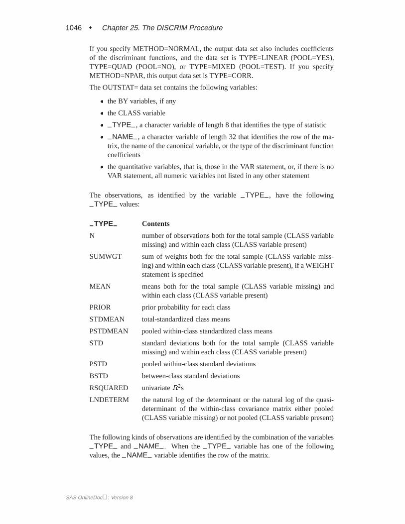
The observations, as identified by the variable–TYPE– , have the following
–TYPE– values:
–TYPE– Contents
N number of observations both for the total sample (CLASS variablemissing) and within each class (CLASS variable present)
SUMWGT sum of weights both for the total sample (CLASS variable miss-ing) and within each class (CLASS variable present), if a WEIGHTstatement is specified
MEAN means both for the total sample (CLASS variable missing) andwithin each class (CLASS variable present)
PRIOR prior probability for each class
STDMEAN total-standardized class means
PSTDMEAN pooled within-class standardized class means
STD standard deviations both for the total sample (CLASS variablemissing) and within each class (CLASS variable present)
PSTD pooled within-class standard deviations
BSTD between-class standard deviations
RSQUARED univariateR2s
LNDETERM the natural log of the determinant or the natural log of the quasi-determinant of the within-class covariance matrix either pooled(CLASS variable missing) or not pooled (CLASS variable present)
The following kinds of observations are identified by the combination of the variables
–TYPE– and –NAME– . When the–TYPE– variable has one of the followingvalues, the–NAME– variable identifies the row of the matrix.
SAS OnlineDoc: Version 8
Output Data Sets � 1047
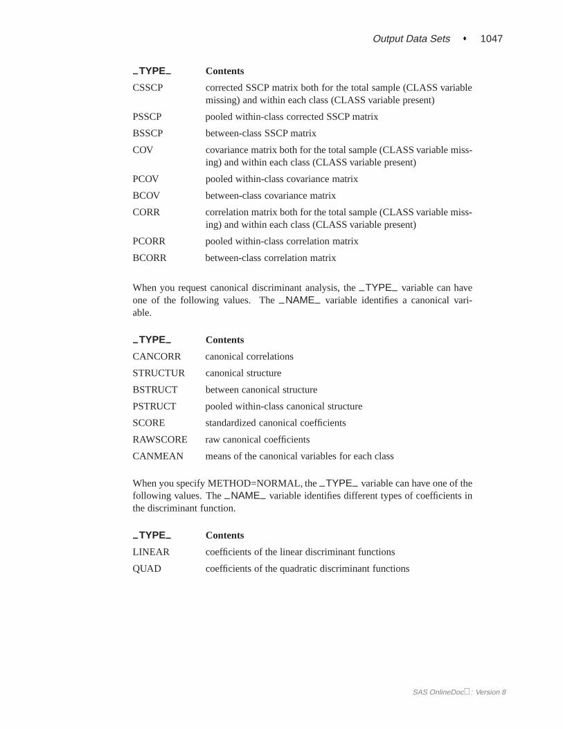
–TYPE– Contents
CSSCP corrected SSCP matrix both for the total sample (CLASS variablemissing) and within each class (CLASS variable present)
PSSCP pooled within-class corrected SSCP matrix
BSSCP between-class SSCP matrix
COV covariance matrix both for the total sample (CLASS variable miss-ing) and within each class (CLASS variable present)
PCOV pooled within-class covariance matrix
BCOV between-class covariance matrix
CORR correlation matrix both for the total sample (CLASS variable miss-ing) and within each class (CLASS variable present)
PCORR pooled within-class correlation matrix
BCORR between-class correlation matrix
When you request canonical discriminant analysis, the–TYPE– variable can haveone of the following values. The–NAME– variable identifies a canonical vari-able.
–TYPE– Contents
CANCORR canonical correlations
STRUCTUR canonical structure
BSTRUCT between canonical structure
PSTRUCT pooled within-class canonical structure
SCORE standardized canonical coefficients
RAWSCORE raw canonical coefficients
CANMEAN means of the canonical variables for each class
When you specify METHOD=NORMAL, the–TYPE– variable can have one of thefollowing values. The–NAME– variable identifies different types of coefficients inthe discriminant function.
–TYPE– Contents
LINEAR coefficients of the linear discriminant functions
QUAD coefficients of the quadratic discriminant functions
SAS OnlineDoc: Version 8
1048 � Chapter 25. The DISCRIM Procedure
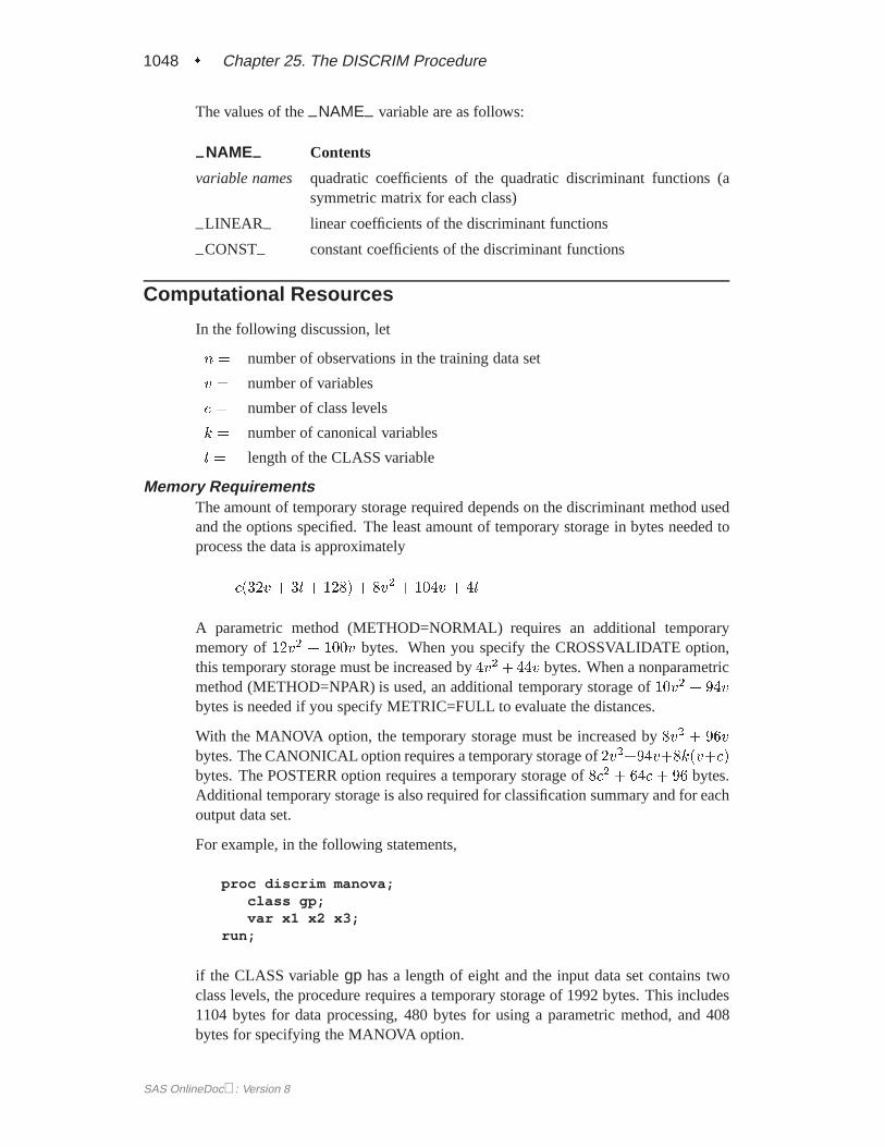
The values of the–NAME– variable are as follows:
–NAME– Contents
variable names quadratic coefficients of the quadratic discriminant functions (asymmetric matrix for each class)
–LINEAR– linear coefficients of the discriminant functions
–CONST– constant coefficients of the discriminant functions
Computational Resources
In the following discussion, let
n = number of observations in the training data set
v = number of variables
c = number of class levels
k = number of canonical variables
l = length of the CLASS variable
Memory RequirementsThe amount of temporary storage required depends on the discriminant method usedand the options specified. The least amount of temporary storage in bytes needed toprocess the data is approximately
c(32v + 3l + 128) + 8v2 + 104v + 4l
A parametric method (METHOD=NORMAL) requires an additional temporarymemory of12v2 + 100v bytes. When you specify the CROSSVALIDATE option,this temporary storage must be increased by4v2+44v bytes. When a nonparametricmethod (METHOD=NPAR) is used, an additional temporary storage of10v2 + 94vbytes is needed if you specify METRIC=FULL to evaluate the distances.
With the MANOVA option, the temporary storage must be increased by8v2 + 96vbytes. The CANONICAL option requires a temporary storage of2v2+94v+8k(v+c)bytes. The POSTERR option requires a temporary storage of8c2 + 64c + 96 bytes.Additional temporary storage is also required for classification summary and for eachoutput data set.
For example, in the following statements,
proc discrim manova;class gp;var x1 x2 x3;
run;
if the CLASS variablegp has a length of eight and the input data set contains twoclass levels, the procedure requires a temporary storage of 1992 bytes. This includes1104 bytes for data processing, 480 bytes for using a parametric method, and 408bytes for specifying the MANOVA option.
SAS OnlineDoc: Version 8
Displayed Output � 1049
Time RequirementsThe following factors determine the time requirements of discriminant analysis.
� The time needed for reading the data and computing covariance matrices isproportional tonv2. PROC DISCRIM must also look up each class level in thelist. This is faster if the data are sorted by the CLASS variable. The time forlooking up class levels is proportional to a value ranging fromn to n ln(c).
� The time for inverting a covariance matrix is proportional tov3.
� With a parametric method, the time required to classify each observation isproportional tocv for a linear discriminant function and is proportional tocv2
for a quadratic discriminant function. When you specify the CROSSVALI-DATE option, the discriminant function is updated for each observation in theclassification. A substantial amount of time is required.
� With a nonparametric method, the data are stored in a tree structure (Friedman,Bentley, and Finkel 1977). The time required to organize the observations intothe tree structure is proportional tonv ln(n). The time for performing each treesearch is proportional toln(n). When you specify the normal KERNEL= op-tion, all observations in the training sample contribute to the density estimationand more computer time is needed.
� The time required for the canonical discriminant analysis is proportional tov3.
Each of the preceding factors has a different machine-dependent constant of propor-tionality.
Displayed Output
The displayed output from PROC DISCRIM includes the following:
� Class Level Information, including the values of the classification variable,Variable Name constructed from each class value, the Frequency and Weightof each value, its Proportion in the total sample, and the Prior Probability foreach class level.
Optional output includes the following:
� Within-Class SSCP Matrices for each group
� Pooled Within-Class SSCP Matrix
� Between-Class SSCP Matrix
� Total-Sample SSCP Matrix
� Within-Class Covariance Matrices,St, for each group
� Pooled Within-Class Covariance Matrix,Sp
� Between-Class Covariance Matrix, equal to the between-class SSCP matrixdivided byn(c � 1)=c, wheren is the number of observations andc is thenumber of classes
SAS OnlineDoc: Version 8

1050 � Chapter 25. The DISCRIM Procedure
� Total-Sample Covariance Matrix
� Within-Class Correlation Coefficients andPr > jrj to test the hypothesis thatthe within-class population correlation coefficients are zero
� Pooled Within-Class Correlation Coefficients andPr > jrj to test the hypoth-esis that the partial population correlation coefficients are zero
� Between-Class Correlation Coefficients andPr > jrj to test the hypothesis thatthe between-class population correlation coefficients are zero
� Total-Sample Correlation Coefficients andPr > jrj to test the hypothesis thatthe total population correlation coefficients are zero
� Simple descriptive Statistics includingN (the number of observations), Sum,Mean, Variance, and Standard Deviation both for the total sample and withineach class
� Total-Sample Standardized Class Means, obtained by subtracting the grandmean from each class mean and dividing by the total sample standard devi-ation
� Pooled Within-Class Standardized Class Means, obtained by subtracting thegrand mean from each class mean and dividing by the pooled within-class stan-dard deviation
� Pairwise Squared Distances Between Groups
� Univariate Test Statistics, including Total-Sample Standard Deviations, PooledWithin-Class Standard Deviations, Between-Class Standard Deviations,R2,R2=(1 � R2), F , andPr > F (univariateF values and probability levels forone-way analyses of variance)
� Multivariate Statistics andF Approximations, including Wilks’ Lambda, Pil-lai’s Trace, Hotelling-Lawley Trace, and Roy’s Greatest Root withF approx-imations, degrees of freedom (Num DF and Den DF), and probability values(Pr > F ). Each of these four multivariate statistics tests the hypothesis thatthe class means are equal in the population. See Chapter 3, “Introduction toRegression Procedures,” for more information.
If you specify METHOD=NORMAL, the following three statistics are displayed:
� Covariance Matrix Information, including Covariance Matrix Rank and Natu-ral Log of Determinant of the Covariance Matrix for each group (POOL=TEST,POOL=NO) and for the pooled within-group (POOL=TEST, POOL=YES)
� Optionally, Test of Homogeneity of Within Covariance Matrices (the resultsof a chi-square test of homogeneity of the within-group covariance matrices)(Morrison 1976; Kendall, Stuart, and Ord 1983; Anderson 1984)
� Pairwise Generalized Squared Distances Between Groups
SAS OnlineDoc: Version 8
Displayed Output � 1051
If the CANONICAL option is specified, the displayed output contains these statistics:
� Canonical Correlations
� Adjusted Canonical Correlations (Lawley 1959). These are asymptotically lessbiased than the raw correlations and can be negative. The adjusted canonicalcorrelations may not be computable and are displayed as missing values if twocanonical correlations are nearly equal or if some are close to zero. A miss-ing value is also displayed if an adjusted canonical correlation is larger than aprevious adjusted canonical correlation.
� Approximate Standard Error of the canonical correlations
� Squared Canonical Correlations
� Eigenvalues ofE�1H. Each eigenvalue is equal to�2=(1 � �2), where�2 isthe corresponding squared canonical correlation and can be interpreted as theratio of between-class variation to within-class variation for the correspond-ing canonical variable. The table includes Eigenvalues, Differences betweensuccessive eigenvalues, the Proportion of the sum of the eigenvalues, and theCumulative proportion.
� Likelihood Ratio for the hypothesis that the current canonical correlation andall smaller ones are zero in the population. The likelihood ratio for all canonicalcorrelations equals Wilks’ lambda.
� ApproximateF statistic based on Rao’s approximation to the distribution ofthe likelihood ratio (Rao 1973, p. 556; Kshirsagar 1972, p. 326)
� Num DF (numerator degrees of freedom), Den DF (denominator degrees offreedom), andPr > F , the probability level associated with theF statistic
The following statistic concerns the classification criterion:
� the Linear Discriminant Function, but only if you specify METHOD=NORMALand the pooled covariance matrix is used to calculate the (generalized) squareddistances
When the input DATA= data set is an ordinary SAS data set, the displayed outputincludes the following:
� Optionally, the Resubstitution Results including Obs, the observation number(if an ID statement is included, the values of the ID variable are displayedinstead of the observation number), the actual group for the observation, thegroup into which the developed criterion would classify it, and the PosteriorProbability of its Membership in each group
� Resubstitution Summary, a summary of the performance of the classificationcriterion based on resubstitution classification results
� Error Count Estimate of the resubstitution classification results
SAS OnlineDoc: Version 8
1052 � Chapter 25. The DISCRIM Procedure
� Optionally, Posterior Probability Error Rate Estimates of the resubstitutionclassification results
If you specify the CROSSVALIDATE option, the displayed output contains thesestatistics:
� Optionally, the Cross-validation Results including Obs, the observation number(if an ID statement is included, the values of the ID variable are displayedinstead of the observation number), the actual group for the observation, thegroup into which the developed criterion would classify it, and the PosteriorProbability of its Membership in each group
� Cross-validation Summary, a summary of the performance of the classificationcriterion based on cross validation classification results
� Error Count Estimate of the cross validation classification results
� Optionally, Posterior Probability Error Rate Estimates of the cross validationclassification results
If you specify the TESTDATA= option, the displayed output contains these statistics:
� Optionally, the Classification Results including Obs, the observation number(if a TESTID statement is included, the values of the ID variable are displayedinstead of the observation number), the actual group for the observation (ifa TESTCLASS statement is included), the group into which the developedcriterion would classify it, and the Posterior Probability of its Membership ineach group
� Classification Summary, a summary of the performance of the classificationcriterion
� Error Count Estimate of the test data classification results
� Optionally, Posterior Probability Error Rate Estimates of the test data classifi-cation results
ODS Table Names
PROC DISCRIM assigns a name to each table it creates. You can use these namesto reference the table when using the Output Delivery System (ODS) to select tablesand create output data sets. These names are listed in the following table. For moreinformation on ODS, see Chapter 15, “Using the Output Delivery System.”
SAS OnlineDoc: Version 8
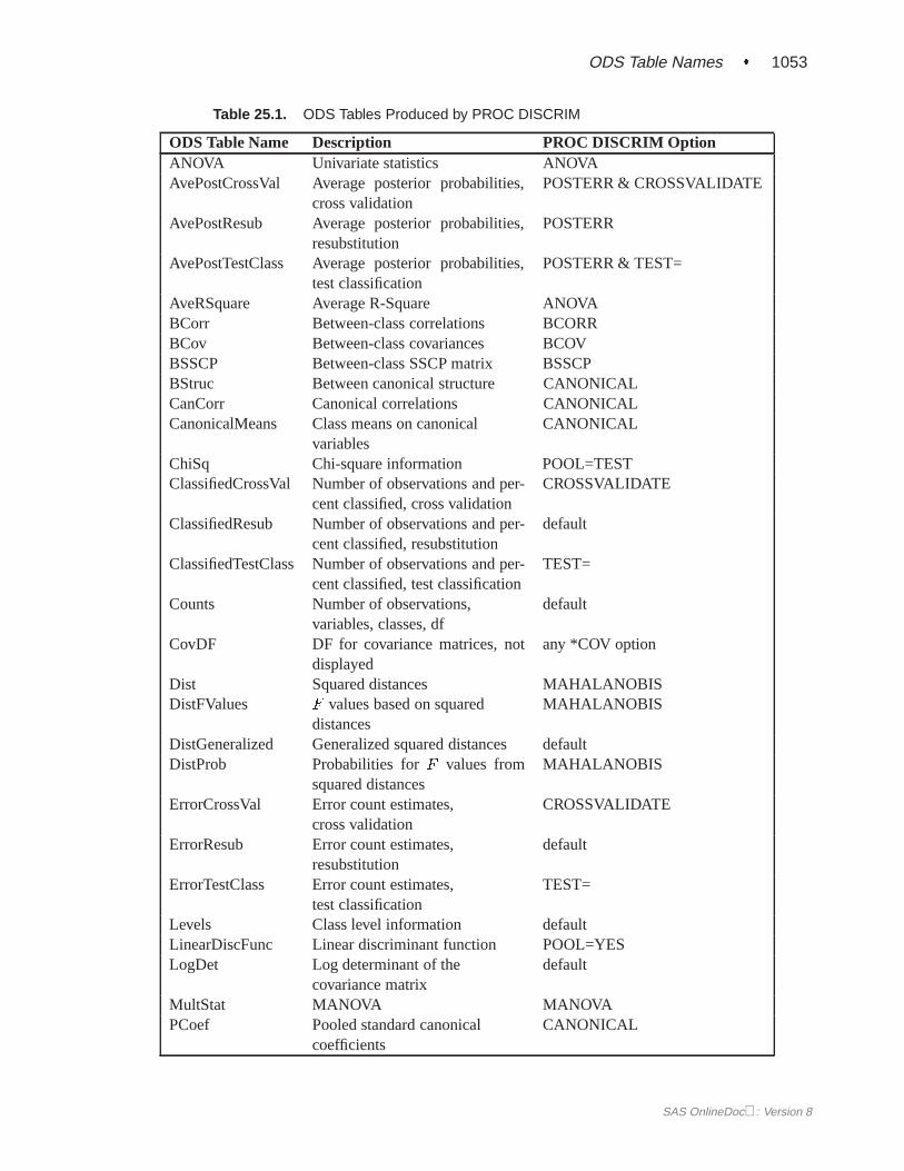
ODS Table Names � 1053
Table 25.1. ODS Tables Produced by PROC DISCRIM
ODS Table Name Description PROC DISCRIM OptionANOVA Univariate statistics ANOVAAvePostCrossVal Average posterior probabilities,
cross validationPOSTERR & CROSSVALIDATE
AvePostResub Average posterior probabilities,resubstitution
POSTERR
AvePostTestClass Average posterior probabilities,test classification
POSTERR & TEST=
AveRSquare Average R-Square ANOVABCorr Between-class correlations BCORRBCov Between-class covariances BCOVBSSCP Between-class SSCP matrix BSSCPBStruc Between canonical structure CANONICALCanCorr Canonical correlations CANONICALCanonicalMeans Class means on canonical
variablesCANONICAL
ChiSq Chi-square information POOL=TESTClassifiedCrossVal Number of observations and per-
cent classified, cross validationCROSSVALIDATE
ClassifiedResub Number of observations and per-cent classified, resubstitution
default
ClassifiedTestClass Number of observations and per-cent classified, test classification
TEST=
Counts Number of observations,variables, classes, df
default
CovDF DF for covariance matrices, notdisplayed
any *COV option
Dist Squared distances MAHALANOBISDistFValues F values based on squared
distancesMAHALANOBIS
DistGeneralized Generalized squared distances defaultDistProb Probabilities forF values from
squared distancesMAHALANOBIS
ErrorCrossVal Error count estimates,cross validation
CROSSVALIDATE
ErrorResub Error count estimates,resubstitution
default
ErrorTestClass Error count estimates,test classification
TEST=
Levels Class level information defaultLinearDiscFunc Linear discriminant function POOL=YESLogDet Log determinant of the
covariance matrixdefault
MultStat MANOVA MANOVAPCoef Pooled standard canonical
coefficientsCANONICAL
SAS OnlineDoc: Version 8
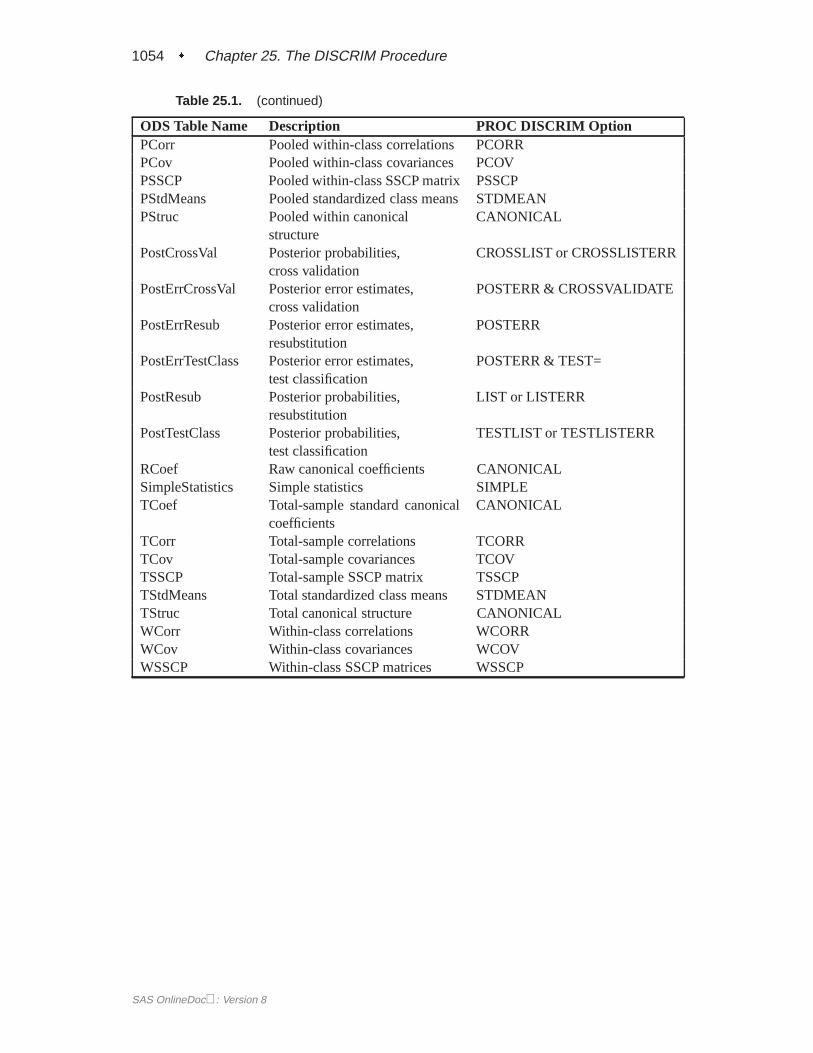
1054 � Chapter 25. The DISCRIM Procedure
Table 25.1. (continued)
ODS Table Name Description PROC DISCRIM OptionPCorr Pooled within-class correlations PCORRPCov Pooled within-class covariances PCOVPSSCP Pooled within-class SSCP matrix PSSCPPStdMeans Pooled standardized class means STDMEANPStruc Pooled within canonical
structureCANONICAL
PostCrossVal Posterior probabilities,cross validation
CROSSLIST or CROSSLISTERR
PostErrCrossVal Posterior error estimates,cross validation
POSTERR & CROSSVALIDATE
PostErrResub Posterior error estimates,resubstitution
POSTERR
PostErrTestClass Posterior error estimates,test classification
POSTERR & TEST=
PostResub Posterior probabilities,resubstitution
LIST or LISTERR
PostTestClass Posterior probabilities,test classification
TESTLIST or TESTLISTERR
RCoef Raw canonical coefficients CANONICALSimpleStatistics Simple statistics SIMPLETCoef Total-sample standard canonical
coefficientsCANONICAL
TCorr Total-sample correlations TCORRTCov Total-sample covariances TCOVTSSCP Total-sample SSCP matrix TSSCPTStdMeans Total standardized class means STDMEANTStruc Total canonical structure CANONICALWCorr Within-class correlations WCORRWCov Within-class covariances WCOVWSSCP Within-class SSCP matrices WSSCP
SAS OnlineDoc: Version 8
Example 25.1. Univariate Density Estimates and Posteriors � 1055
Examples
The iris data published by Fisher (1936) are widely used for examples in discriminantanalysis and cluster analysis. The sepal length, sepal width, petal length, and petalwidth are measured in millimeters on fifty iris specimens from each of three species,Iris setosa, I. versicolor, and I. virginica. The iris data are used in Example 25.1through Example 25.3.
Example 25.4 and Example 25.5 use remote-sensing data on crops. In this data set,the observations are grouped into five crops: clover, corn, cotton, soybeans, and sugarbeets. Four measures called X1 through X4 make up the descriptive variables.
Example 25.1. Univariate Density Estimates and PosteriorProbabilities
In this example, several discriminant analyses are run with a single quantitative vari-able, petal width, so that density estimates and posterior probabilities can be plottedeasily. The example produces Output 25.1.1 through Output 25.1.5. The GCHARTprocedure is used to display the sample distribution of petal width in the three species.Note the overlap between speciesI. versicolor and I. virginica that the bar chartshows. These statements produce Output 25.1.1:
proc format;value specname
1=’Setosa ’2=’Versicolor’3=’Virginica ’;
run;
data iris;title ’Discriminant Analysis of Fisher (1936) Iris Data’;input SepalLength SepalWidth PetalLength PetalWidth
Species @@;format Species specname.;label SepalLength=’Sepal Length in mm.’
SepalWidth =’Sepal Width in mm.’PetalLength=’Petal Length in mm.’PetalWidth =’Petal Width in mm.’;
symbol = put(Species, specname10.);datalines;
50 33 14 02 1 64 28 56 22 3 65 28 46 15 2 67 31 56 24 363 28 51 15 3 46 34 14 03 1 69 31 51 23 3 62 22 45 15 259 32 48 18 2 46 36 10 02 1 61 30 46 14 2 60 27 51 16 265 30 52 20 3 56 25 39 11 2 65 30 55 18 3 58 27 51 19 368 32 59 23 3 51 33 17 05 1 57 28 45 13 2 62 34 54 23 377 38 67 22 3 63 33 47 16 2 67 33 57 25 3 76 30 66 21 349 25 45 17 3 55 35 13 02 1 67 30 52 23 3 70 32 47 14 264 32 45 15 2 61 28 40 13 2 48 31 16 02 1 59 30 51 18 355 24 38 11 2 63 25 50 19 3 64 32 53 23 3 52 34 14 02 149 36 14 01 1 54 30 45 15 2 79 38 64 20 3 44 32 13 02 167 33 57 21 3 50 35 16 06 1 58 26 40 12 2 44 30 13 02 177 28 67 20 3 63 27 49 18 3 47 32 16 02 1 55 26 44 12 2
SAS OnlineDoc: Version 8
1056 � Chapter 25. The DISCRIM Procedure
50 23 33 10 2 72 32 60 18 3 48 30 14 03 1 51 38 16 02 161 30 49 18 3 48 34 19 02 1 50 30 16 02 1 50 32 12 02 161 26 56 14 3 64 28 56 21 3 43 30 11 01 1 58 40 12 02 151 38 19 04 1 67 31 44 14 2 62 28 48 18 3 49 30 14 02 151 35 14 02 1 56 30 45 15 2 58 27 41 10 2 50 34 16 04 146 32 14 02 1 60 29 45 15 2 57 26 35 10 2 57 44 15 04 150 36 14 02 1 77 30 61 23 3 63 34 56 24 3 58 27 51 19 357 29 42 13 2 72 30 58 16 3 54 34 15 04 1 52 41 15 01 171 30 59 21 3 64 31 55 18 3 60 30 48 18 3 63 29 56 18 349 24 33 10 2 56 27 42 13 2 57 30 42 12 2 55 42 14 02 149 31 15 02 1 77 26 69 23 3 60 22 50 15 3 54 39 17 04 166 29 46 13 2 52 27 39 14 2 60 34 45 16 2 50 34 15 02 144 29 14 02 1 50 20 35 10 2 55 24 37 10 2 58 27 39 12 247 32 13 02 1 46 31 15 02 1 69 32 57 23 3 62 29 43 13 274 28 61 19 3 59 30 42 15 2 51 34 15 02 1 50 35 13 03 156 28 49 20 3 60 22 40 10 2 73 29 63 18 3 67 25 58 18 349 31 15 01 1 67 31 47 15 2 63 23 44 13 2 54 37 15 02 156 30 41 13 2 63 25 49 15 2 61 28 47 12 2 64 29 43 13 251 25 30 11 2 57 28 41 13 2 65 30 58 22 3 69 31 54 21 354 39 13 04 1 51 35 14 03 1 72 36 61 25 3 65 32 51 20 361 29 47 14 2 56 29 36 13 2 69 31 49 15 2 64 27 53 19 368 30 55 21 3 55 25 40 13 2 48 34 16 02 1 48 30 14 01 145 23 13 03 1 57 25 50 20 3 57 38 17 03 1 51 38 15 03 155 23 40 13 2 66 30 44 14 2 68 28 48 14 2 54 34 17 02 151 37 15 04 1 52 35 15 02 1 58 28 51 24 3 67 30 50 17 263 33 60 25 3 53 37 15 02 1;
pattern1 c=red /*v=l1 */;pattern2 c=yellow /*v=empty*/;pattern3 c=blue /*v=r1 */;axis1 label=(angle=90);axis2 value=(height=.6);legend1 frame label=none;
proc gchart data=iris;vbar PetalWidth / subgroup=Species midpoints=0 to 25
raxis=axis1 maxis=axis2 legend=legend1 cframe=ligr;run;
SAS OnlineDoc: Version 8
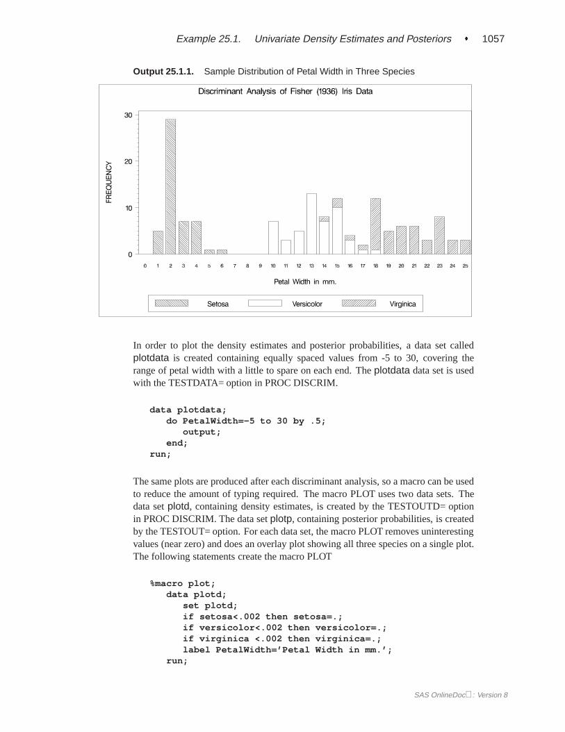
Example 25.1. Univariate Density Estimates and Posteriors � 1057
Output 25.1.1. Sample Distribution of Petal Width in Three Species
In order to plot the density estimates and posterior probabilities, a data set calledplotdata is created containing equally spaced values from -5 to 30, covering therange of petal width with a little to spare on each end. Theplotdata data set is usedwith the TESTDATA= option in PROC DISCRIM.
data plotdata;do PetalWidth=-5 to 30 by .5;
output;end;
run;
The same plots are produced after each discriminant analysis, so a macro can be usedto reduce the amount of typing required. The macro PLOT uses two data sets. Thedata setplotd, containing density estimates, is created by the TESTOUTD= optionin PROC DISCRIM. The data setplotp, containing posterior probabilities, is createdby the TESTOUT= option. For each data set, the macro PLOT removes uninterestingvalues (near zero) and does an overlay plot showing all three species on a single plot.The following statements create the macro PLOT
%macro plot;data plotd;
set plotd;if setosa<.002 then setosa=.;if versicolor<.002 then versicolor=.;if virginica <.002 then virginica=.;label PetalWidth=’Petal Width in mm.’;
run;
SAS OnlineDoc: Version 8
1058 � Chapter 25. The DISCRIM Procedure
symbol1 i=join v=none c=red l=1 /*l=21*/;symbol2 i=join v=none c=yellow l=1 /*l= 1*/;symbol3 i=join v=none c=blue l=1 /*l= 2*/;legend1 label=none frame;axis1 label=(angle=90 ’Density’) order=(0 to .6 by .1);
proc gplot data=plotd;plot setosa*PetalWidth
versicolor*PetalWidthvirginica*PetalWidth/ overlay vaxis=axis1 legend=legend1 frame
cframe=ligr;title3 ’Plot of Estimated Densities’;
run;
data plotp;set plotp;if setosa<.01 then setosa=.;if versicolor<.01 then versicolor=.;if virginica<.01 then virginica=.;label PetalWidth=’Petal Width in mm.’;
run;
axis1 label=(angle=90 ’Posterior Probability’)order=(0 to 1 by .2);
proc gplot data=plotp;plot setosa*PetalWidth
versicolor*PetalWidthvirginica*PetalWidth/ overlay vaxis=axis1 legend=legend1 frame
cframe=ligr;title3 ’Plot of Posterior Probabilities’;
run;%mend;
The first analysis uses normal-theory methods (METHOD=NORMAL) assumingequal variances (POOL=YES) in the three classes. The NOCLASSIFY option sup-presses the resubstitution classification results of the input data set observations. TheCROSSLISTERR option lists the observations that are misclassified under cross val-idation and displays cross validation error-rate estimates. The following statementsproduce Output 25.1.2:
proc discrim data=iris method=normal pool=yestestdata=plotdata testout=plotp testoutd=plotdshort noclassify crosslisterr;
class Species;var PetalWidth;title2 ’Using Normal Density Estimates with Equal Variance’;
run;%plot
SAS OnlineDoc: Version 8
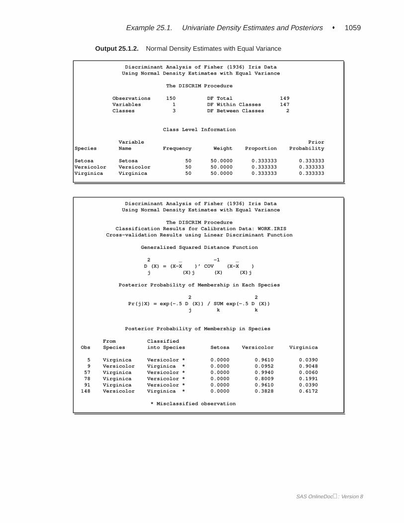
Example 25.1. Univariate Density Estimates and Posteriors � 1059
Output 25.1.2. Normal Density Estimates with Equal Variance
Discriminant Analysis of Fisher (1936) Iris DataUsing Normal Density Estimates with Equal Variance
The DISCRIM Procedure
Observations 150 DF Total 149Variables 1 DF Within Classes 147Classes 3 DF Between Classes 2
Class Level Information
Variable PriorSpecies Name Frequency Weight Proportion Probability
Setosa Setosa 50 50.0000 0.333333 0.333333Versicolor Versicolor 50 50.0000 0.333333 0.333333Virginica Virginica 50 50.0000 0.333333 0.333333
Discriminant Analysis of Fisher (1936) Iris DataUsing Normal Density Estimates with Equal Variance
The DISCRIM ProcedureClassification Results for Calibration Data: WORK.IRIS
Cross-validation Results using Linear Discriminant Function
Generalized Squared Distance Function
2 _ -1 _D (X) = (X-X )’ COV (X-X )
j (X)j (X) (X)j
Posterior Probability of Membership in Each Species
2 2Pr(j|X) = exp(-.5 D (X)) / SUM exp(-.5 D (X))
j k k
Posterior Probability of Membership in Species
From ClassifiedObs Species into Species Setosa Versicolor Virginica
5 Virginica Versicolor * 0.0000 0.9610 0.03909 Versicolor Virginica * 0.0000 0.0952 0.9048
57 Virginica Versicolor * 0.0000 0.9940 0.006078 Virginica Versicolor * 0.0000 0.8009 0.199191 Virginica Versicolor * 0.0000 0.9610 0.0390
148 Versicolor Virginica * 0.0000 0.3828 0.6172
* Misclassified observation
SAS OnlineDoc: Version 8
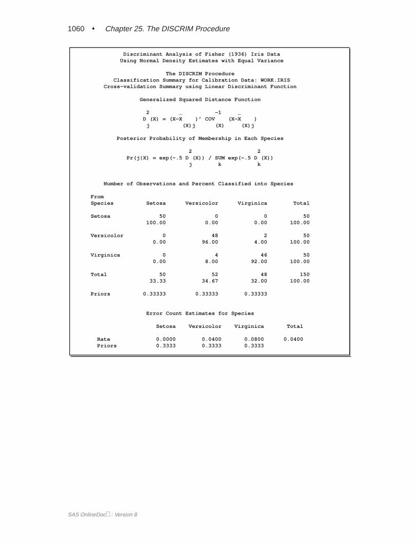
1060 � Chapter 25. The DISCRIM Procedure
Discriminant Analysis of Fisher (1936) Iris DataUsing Normal Density Estimates with Equal Variance
The DISCRIM ProcedureClassification Summary for Calibration Data: WORK.IRIS
Cross-validation Summary using Linear Discriminant Function
Generalized Squared Distance Function
2 _ -1 _D (X) = (X-X )’ COV (X-X )
j (X)j (X) (X)j
Posterior Probability of Membership in Each Species
2 2Pr(j|X) = exp(-.5 D (X)) / SUM exp(-.5 D (X))
j k k
Number of Observations and Percent Classified into Species
FromSpecies Setosa Versicolor Virginica Total
Setosa 50 0 0 50100.00 0.00 0.00 100.00
Versicolor 0 48 2 500.00 96.00 4.00 100.00
Virginica 0 4 46 500.00 8.00 92.00 100.00
Total 50 52 48 15033.33 34.67 32.00 100.00
Priors 0.33333 0.33333 0.33333
Error Count Estimates for Species
Setosa Versicolor Virginica Total
Rate 0.0000 0.0400 0.0800 0.0400Priors 0.3333 0.3333 0.3333
SAS OnlineDoc: Version 8
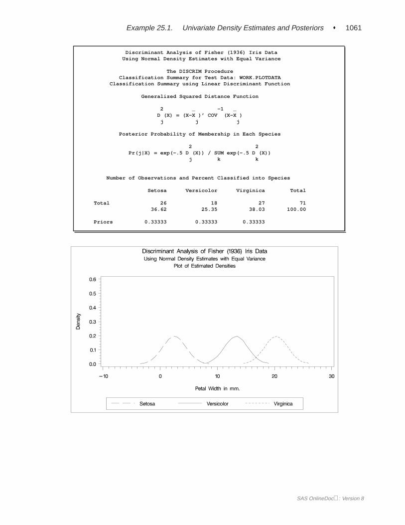
Example 25.1. Univariate Density Estimates and Posteriors � 1061
Discriminant Analysis of Fisher (1936) Iris DataUsing Normal Density Estimates with Equal Variance
The DISCRIM ProcedureClassification Summary for Test Data: WORK.PLOTDATA
Classification Summary using Linear Discriminant Function
Generalized Squared Distance Function
2 _ -1 _D (X) = (X-X )’ COV (X-X )
j j j
Posterior Probability of Membership in Each Species
2 2Pr(j|X) = exp(-.5 D (X)) / SUM exp(-.5 D (X))
j k k
Number of Observations and Percent Classified into Species
Setosa Versicolor Virginica Total
Total 26 18 27 7136.62 25.35 38.03 100.00
Priors 0.33333 0.33333 0.33333
SAS OnlineDoc: Version 8
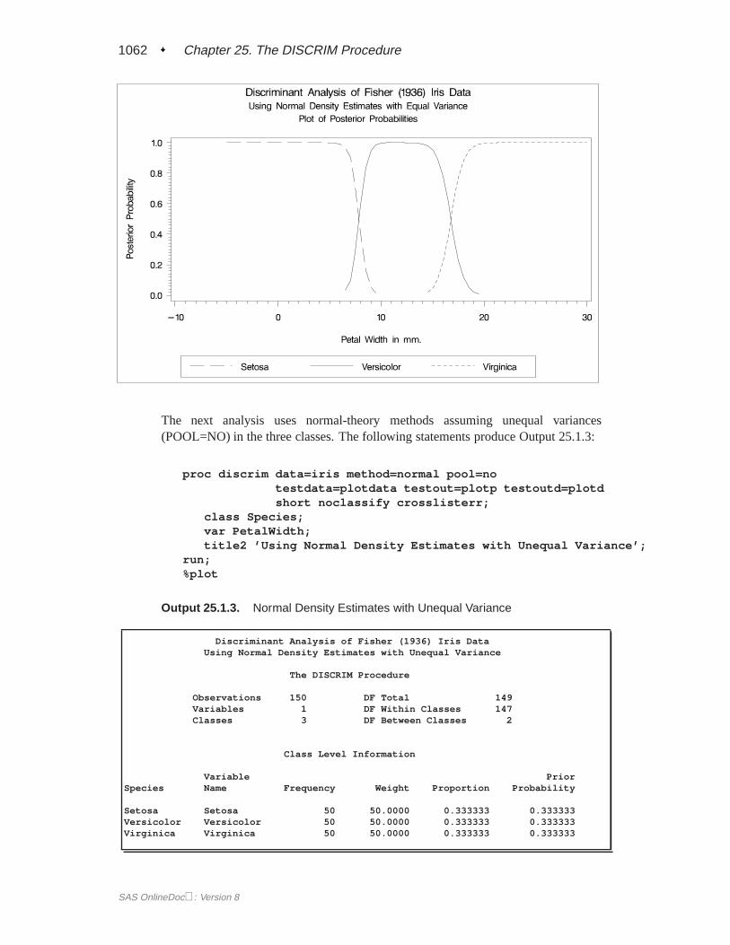
1062 � Chapter 25. The DISCRIM Procedure
The next analysis uses normal-theory methods assuming unequal variances(POOL=NO) in the three classes. The following statements produce Output 25.1.3:
proc discrim data=iris method=normal pool=notestdata=plotdata testout=plotp testoutd=plotdshort noclassify crosslisterr;
class Species;var PetalWidth;title2 ’Using Normal Density Estimates with Unequal Variance’;
run;%plot
Output 25.1.3. Normal Density Estimates with Unequal Variance
Discriminant Analysis of Fisher (1936) Iris DataUsing Normal Density Estimates with Unequal Variance
The DISCRIM Procedure
Observations 150 DF Total 149Variables 1 DF Within Classes 147Classes 3 DF Between Classes 2
Class Level Information
Variable PriorSpecies Name Frequency Weight Proportion Probability
Setosa Setosa 50 50.0000 0.333333 0.333333Versicolor Versicolor 50 50.0000 0.333333 0.333333Virginica Virginica 50 50.0000 0.333333 0.333333
SAS OnlineDoc: Version 8
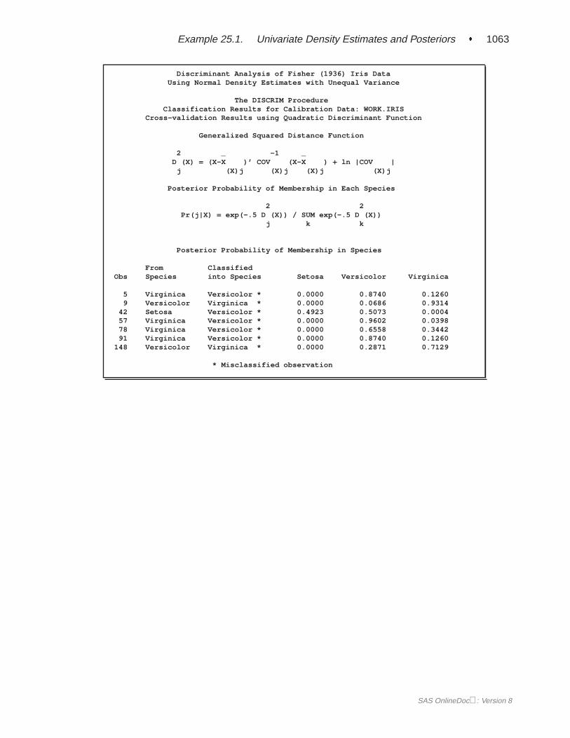
Example 25.1. Univariate Density Estimates and Posteriors � 1063
Discriminant Analysis of Fisher (1936) Iris DataUsing Normal Density Estimates with Unequal Variance
The DISCRIM ProcedureClassification Results for Calibration Data: WORK.IRIS
Cross-validation Results using Quadratic Discriminant Function
Generalized Squared Distance Function
2 _ -1 _D (X) = (X-X )’ COV (X-X ) + ln |COV |
j (X)j (X)j (X)j (X)j
Posterior Probability of Membership in Each Species
2 2Pr(j|X) = exp(-.5 D (X)) / SUM exp(-.5 D (X))
j k k
Posterior Probability of Membership in Species
From ClassifiedObs Species into Species Setosa Versicolor Virginica
5 Virginica Versicolor * 0.0000 0.8740 0.12609 Versicolor Virginica * 0.0000 0.0686 0.9314
42 Setosa Versicolor * 0.4923 0.5073 0.000457 Virginica Versicolor * 0.0000 0.9602 0.039878 Virginica Versicolor * 0.0000 0.6558 0.344291 Virginica Versicolor * 0.0000 0.8740 0.1260
148 Versicolor Virginica * 0.0000 0.2871 0.7129
* Misclassified observation
SAS OnlineDoc: Version 8
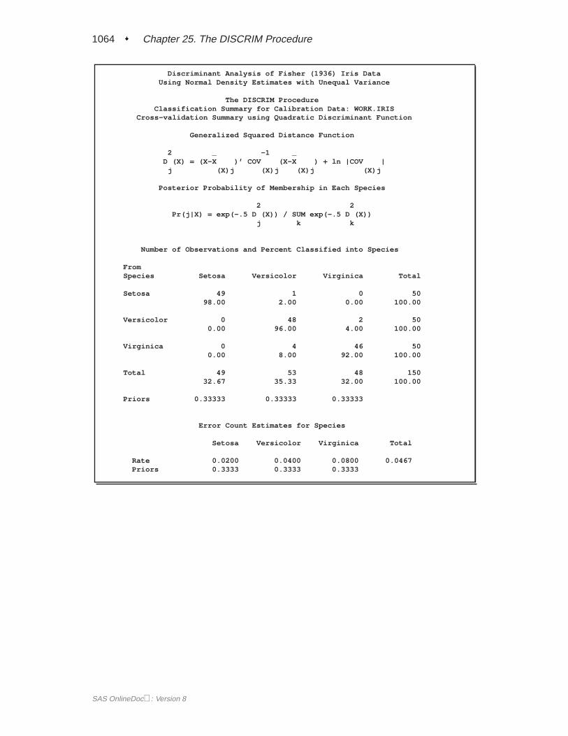
1064 � Chapter 25. The DISCRIM Procedure
Discriminant Analysis of Fisher (1936) Iris DataUsing Normal Density Estimates with Unequal Variance
The DISCRIM ProcedureClassification Summary for Calibration Data: WORK.IRIS
Cross-validation Summary using Quadratic Discriminant Function
Generalized Squared Distance Function
2 _ -1 _D (X) = (X-X )’ COV (X-X ) + ln |COV |
j (X)j (X)j (X)j (X)j
Posterior Probability of Membership in Each Species
2 2Pr(j|X) = exp(-.5 D (X)) / SUM exp(-.5 D (X))
j k k
Number of Observations and Percent Classified into Species
FromSpecies Setosa Versicolor Virginica Total
Setosa 49 1 0 5098.00 2.00 0.00 100.00
Versicolor 0 48 2 500.00 96.00 4.00 100.00
Virginica 0 4 46 500.00 8.00 92.00 100.00
Total 49 53 48 15032.67 35.33 32.00 100.00
Priors 0.33333 0.33333 0.33333
Error Count Estimates for Species
Setosa Versicolor Virginica Total
Rate 0.0200 0.0400 0.0800 0.0467Priors 0.3333 0.3333 0.3333
SAS OnlineDoc: Version 8
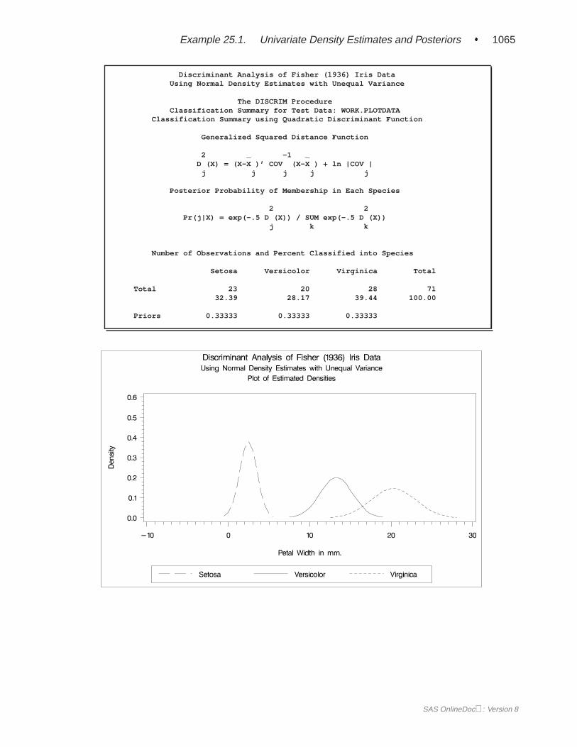
Example 25.1. Univariate Density Estimates and Posteriors � 1065
Discriminant Analysis of Fisher (1936) Iris DataUsing Normal Density Estimates with Unequal Variance
The DISCRIM ProcedureClassification Summary for Test Data: WORK.PLOTDATA
Classification Summary using Quadratic Discriminant Function
Generalized Squared Distance Function
2 _ -1 _D (X) = (X-X )’ COV (X-X ) + ln |COV |
j j j j j
Posterior Probability of Membership in Each Species
2 2Pr(j|X) = exp(-.5 D (X)) / SUM exp(-.5 D (X))
j k k
Number of Observations and Percent Classified into Species
Setosa Versicolor Virginica Total
Total 23 20 28 7132.39 28.17 39.44 100.00
Priors 0.33333 0.33333 0.33333
SAS OnlineDoc: Version 8
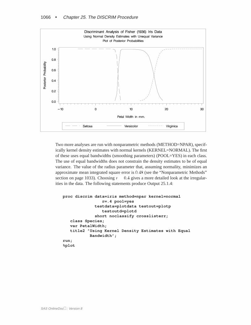
1066 � Chapter 25. The DISCRIM Procedure
Two more analyses are run with nonparametric methods (METHOD=NPAR), specif-ically kernel density estimates with normal kernels (KERNEL=NORMAL). The firstof these uses equal bandwidths (smoothing parameters) (POOL=YES) in each class.The use of equal bandwidths does not constrain the density estimates to be of equalvariance. The value of the radius parameter that, assuming normality, minimizes anapproximate mean integrated square error is0:48 (see the “Nonparametric Methods”section on page 1033). Choosingr = 0:4 gives a more detailed look at the irregular-ities in the data. The following statements produce Output 25.1.4:
proc discrim data=iris method=npar kernel=normalr=.4 pool=yes
testdata=plotdata testout=plotptestoutd=plotd
short noclassify crosslisterr;class Species;var PetalWidth;title2 ’Using Kernel Density Estimates with Equal
Bandwidth’;run;%plot
SAS OnlineDoc: Version 8
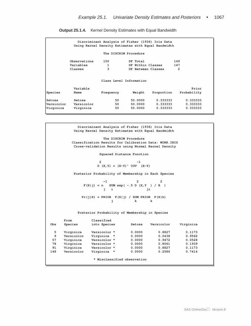
Example 25.1. Univariate Density Estimates and Posteriors � 1067
Output 25.1.4. Kernel Density Estimates with Equal Bandwidth
Discriminant Analysis of Fisher (1936) Iris DataUsing Kernel Density Estimates with Equal Bandwidth
The DISCRIM Procedure
Observations 150 DF Total 149Variables 1 DF Within Classes 147Classes 3 DF Between Classes 2
Class Level Information
Variable PriorSpecies Name Frequency Weight Proportion Probability
Setosa Setosa 50 50.0000 0.333333 0.333333Versicolor Versicolor 50 50.0000 0.333333 0.333333Virginica Virginica 50 50.0000 0.333333 0.333333
Discriminant Analysis of Fisher (1936) Iris DataUsing Kernel Density Estimates with Equal Bandwidth
The DISCRIM ProcedureClassification Results for Calibration Data: WORK.IRIS
Cross-validation Results using Normal Kernel Density
Squared Distance Function
2 -1D (X,Y) = (X-Y)’ COV (X-Y)
Posterior Probability of Membership in Each Species
-1 2 2F(X|j) = n SUM exp( -.5 D (X,Y ) / R )
j i ji
Pr(j|X) = PRIOR F(X|j) / SUM PRIOR F(X|k)j k k
Posterior Probability of Membership in Species
From ClassifiedObs Species into Species Setosa Versicolor Virginica
5 Virginica Versicolor * 0.0000 0.8827 0.11739 Versicolor Virginica * 0.0000 0.0438 0.9562
57 Virginica Versicolor * 0.0000 0.9472 0.052878 Virginica Versicolor * 0.0000 0.8061 0.193991 Virginica Versicolor * 0.0000 0.8827 0.1173
148 Versicolor Virginica * 0.0000 0.2586 0.7414
* Misclassified observation
SAS OnlineDoc: Version 8
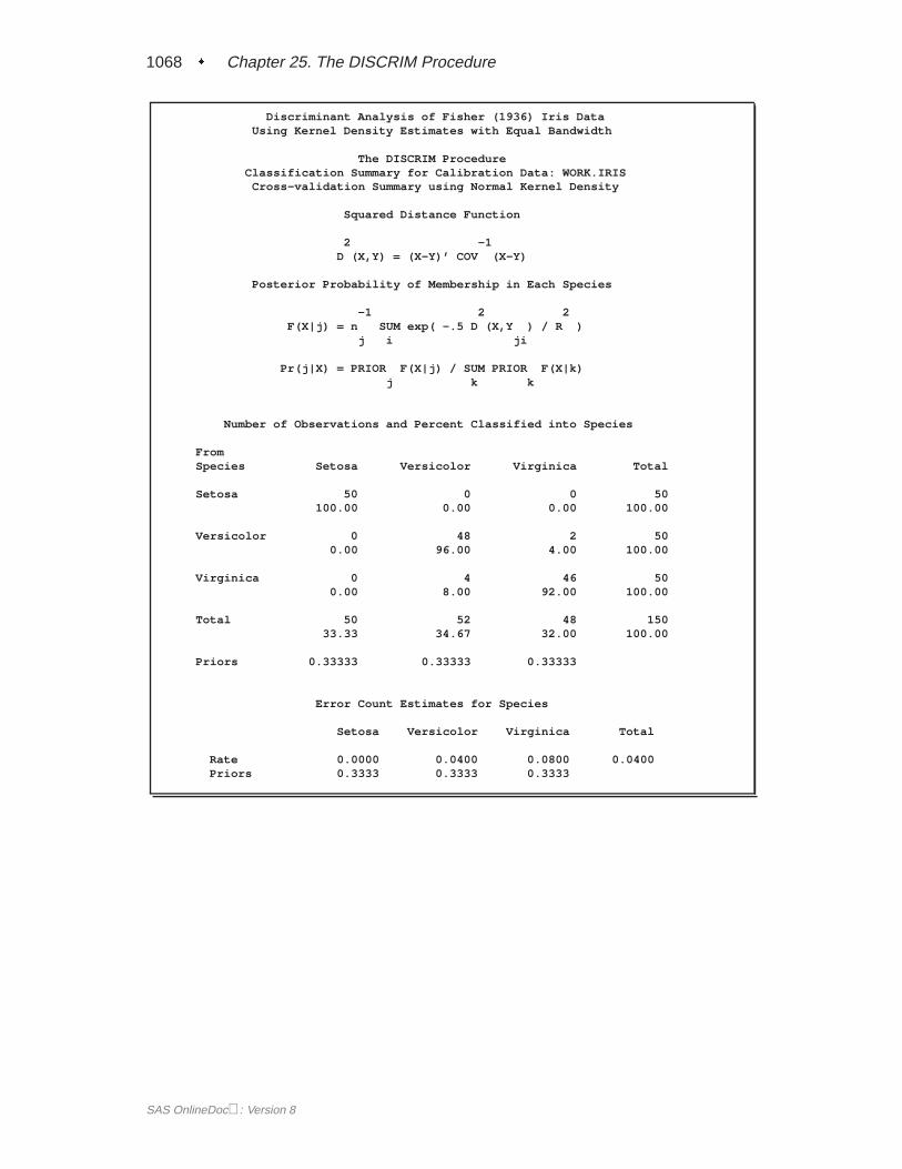
1068 � Chapter 25. The DISCRIM Procedure
Discriminant Analysis of Fisher (1936) Iris DataUsing Kernel Density Estimates with Equal Bandwidth
The DISCRIM ProcedureClassification Summary for Calibration Data: WORK.IRIS
Cross-validation Summary using Normal Kernel Density
Squared Distance Function
2 -1D (X,Y) = (X-Y)’ COV (X-Y)
Posterior Probability of Membership in Each Species
-1 2 2F(X|j) = n SUM exp( -.5 D (X,Y ) / R )
j i ji
Pr(j|X) = PRIOR F(X|j) / SUM PRIOR F(X|k)j k k
Number of Observations and Percent Classified into Species
FromSpecies Setosa Versicolor Virginica Total
Setosa 50 0 0 50100.00 0.00 0.00 100.00
Versicolor 0 48 2 500.00 96.00 4.00 100.00
Virginica 0 4 46 500.00 8.00 92.00 100.00
Total 50 52 48 15033.33 34.67 32.00 100.00
Priors 0.33333 0.33333 0.33333
Error Count Estimates for Species
Setosa Versicolor Virginica Total
Rate 0.0000 0.0400 0.0800 0.0400Priors 0.3333 0.3333 0.3333
SAS OnlineDoc: Version 8
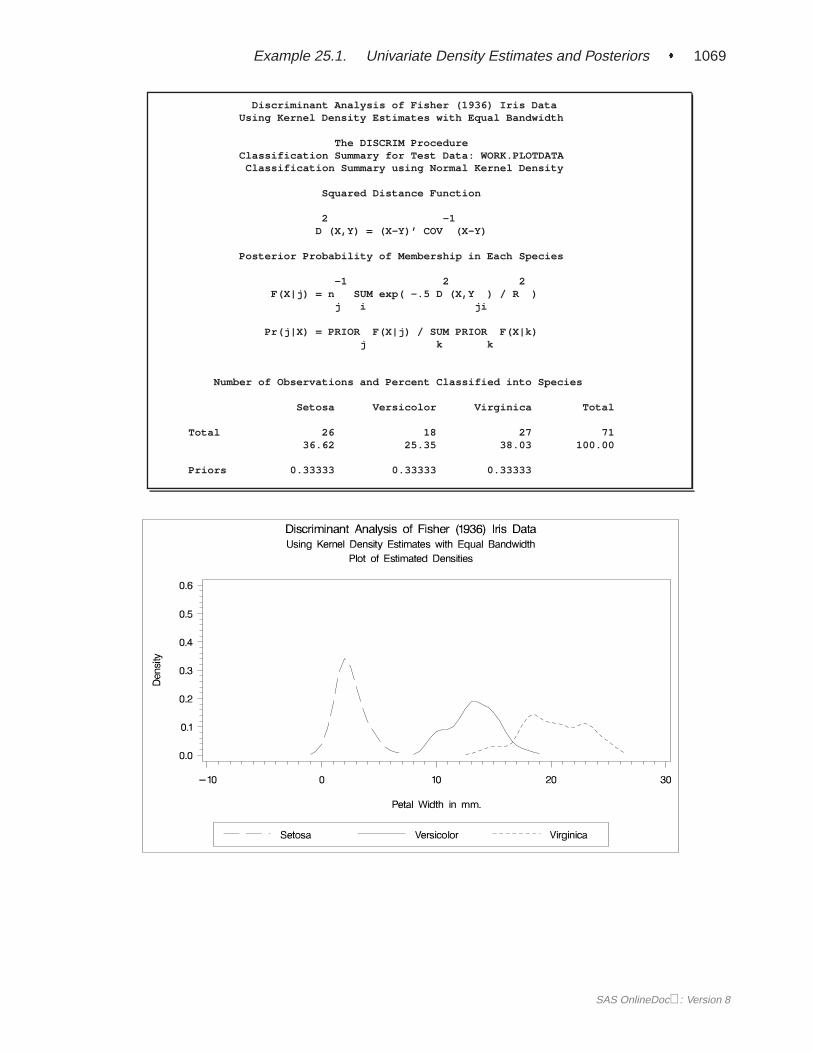
Example 25.1. Univariate Density Estimates and Posteriors � 1069
Discriminant Analysis of Fisher (1936) Iris DataUsing Kernel Density Estimates with Equal Bandwidth
The DISCRIM ProcedureClassification Summary for Test Data: WORK.PLOTDATA
Classification Summary using Normal Kernel Density
Squared Distance Function
2 -1D (X,Y) = (X-Y)’ COV (X-Y)
Posterior Probability of Membership in Each Species
-1 2 2F(X|j) = n SUM exp( -.5 D (X,Y ) / R )
j i ji
Pr(j|X) = PRIOR F(X|j) / SUM PRIOR F(X|k)j k k
Number of Observations and Percent Classified into Species
Setosa Versicolor Virginica Total
Total 26 18 27 7136.62 25.35 38.03 100.00
Priors 0.33333 0.33333 0.33333
SAS OnlineDoc: Version 8
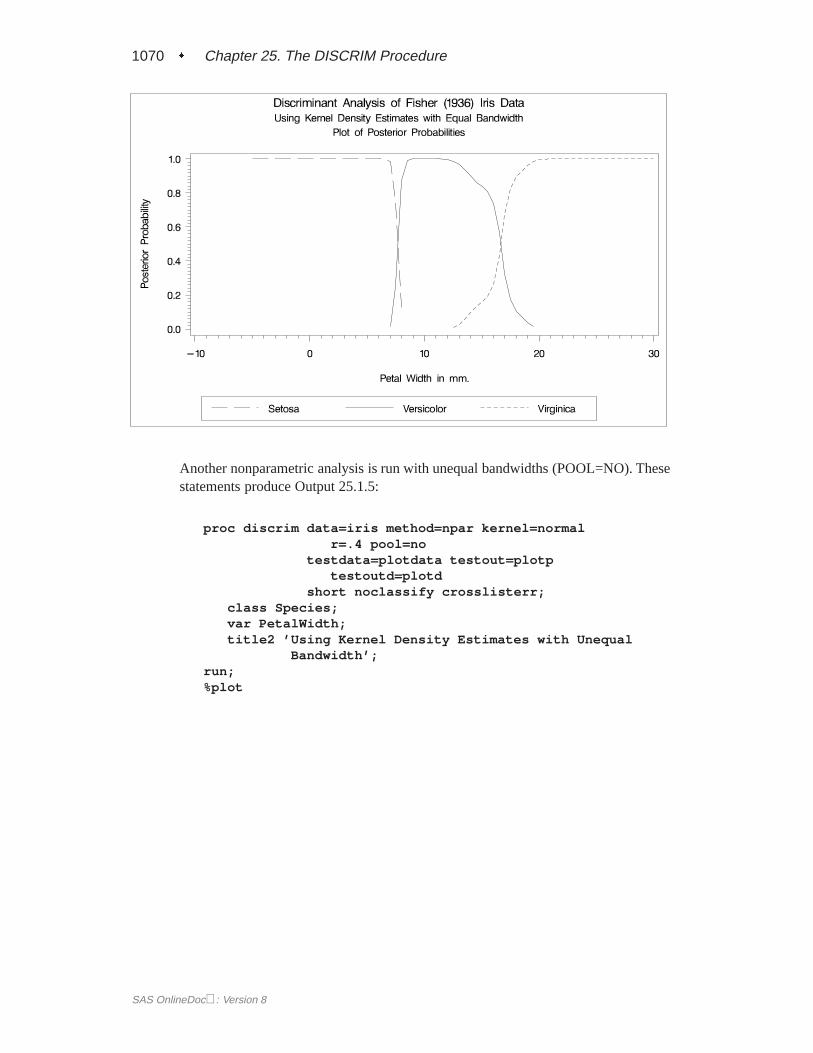
1070 � Chapter 25. The DISCRIM Procedure
Another nonparametric analysis is run with unequal bandwidths (POOL=NO). Thesestatements produce Output 25.1.5:
proc discrim data=iris method=npar kernel=normalr=.4 pool=no
testdata=plotdata testout=plotptestoutd=plotd
short noclassify crosslisterr;class Species;var PetalWidth;title2 ’Using Kernel Density Estimates with Unequal
Bandwidth’;run;%plot
SAS OnlineDoc: Version 8
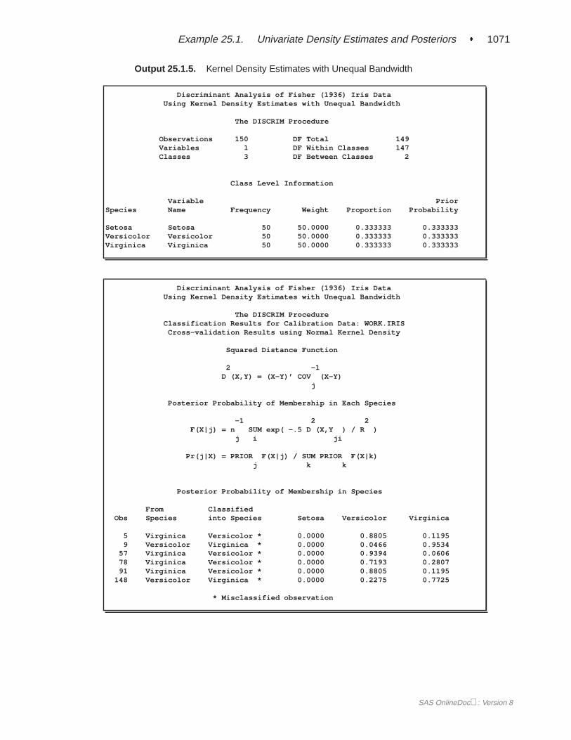
Example 25.1. Univariate Density Estimates and Posteriors � 1071
Output 25.1.5. Kernel Density Estimates with Unequal Bandwidth
Discriminant Analysis of Fisher (1936) Iris DataUsing Kernel Density Estimates with Unequal Bandwidth
The DISCRIM Procedure
Observations 150 DF Total 149Variables 1 DF Within Classes 147Classes 3 DF Between Classes 2
Class Level Information
Variable PriorSpecies Name Frequency Weight Proportion Probability
Setosa Setosa 50 50.0000 0.333333 0.333333Versicolor Versicolor 50 50.0000 0.333333 0.333333Virginica Virginica 50 50.0000 0.333333 0.333333
Discriminant Analysis of Fisher (1936) Iris DataUsing Kernel Density Estimates with Unequal Bandwidth
The DISCRIM ProcedureClassification Results for Calibration Data: WORK.IRIS
Cross-validation Results using Normal Kernel Density
Squared Distance Function
2 -1D (X,Y) = (X-Y)’ COV (X-Y)
j
Posterior Probability of Membership in Each Species
-1 2 2F(X|j) = n SUM exp( -.5 D (X,Y ) / R )
j i ji
Pr(j|X) = PRIOR F(X|j) / SUM PRIOR F(X|k)j k k
Posterior Probability of Membership in Species
From ClassifiedObs Species into Species Setosa Versicolor Virginica
5 Virginica Versicolor * 0.0000 0.8805 0.11959 Versicolor Virginica * 0.0000 0.0466 0.9534
57 Virginica Versicolor * 0.0000 0.9394 0.060678 Virginica Versicolor * 0.0000 0.7193 0.280791 Virginica Versicolor * 0.0000 0.8805 0.1195
148 Versicolor Virginica * 0.0000 0.2275 0.7725
* Misclassified observation
SAS OnlineDoc: Version 8

1072 � Chapter 25. The DISCRIM Procedure
Discriminant Analysis of Fisher (1936) Iris DataUsing Kernel Density Estimates with Unequal Bandwidth
The DISCRIM ProcedureClassification Summary for Calibration Data: WORK.IRIS
Cross-validation Summary using Normal Kernel Density
Squared Distance Function
2 -1D (X,Y) = (X-Y)’ COV (X-Y)
j
Posterior Probability of Membership in Each Species
-1 2 2F(X|j) = n SUM exp( -.5 D (X,Y ) / R )
j i ji
Pr(j|X) = PRIOR F(X|j) / SUM PRIOR F(X|k)j k k
Number of Observations and Percent Classified into Species
FromSpecies Setosa Versicolor Virginica Total
Setosa 50 0 0 50100.00 0.00 0.00 100.00
Versicolor 0 48 2 500.00 96.00 4.00 100.00
Virginica 0 4 46 500.00 8.00 92.00 100.00
Total 50 52 48 15033.33 34.67 32.00 100.00
Priors 0.33333 0.33333 0.33333
Error Count Estimates for Species
Setosa Versicolor Virginica Total
Rate 0.0000 0.0400 0.0800 0.0400Priors 0.3333 0.3333 0.3333
SAS OnlineDoc: Version 8
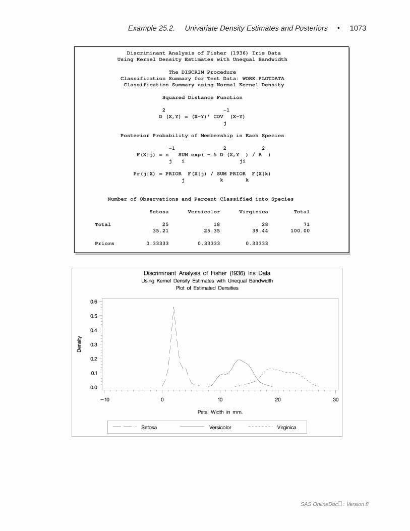
Example 25.2. Univariate Density Estimates and Posteriors � 1073
Discriminant Analysis of Fisher (1936) Iris DataUsing Kernel Density Estimates with Unequal Bandwidth
The DISCRIM ProcedureClassification Summary for Test Data: WORK.PLOTDATA
Classification Summary using Normal Kernel Density
Squared Distance Function
2 -1D (X,Y) = (X-Y)’ COV (X-Y)
j
Posterior Probability of Membership in Each Species
-1 2 2F(X|j) = n SUM exp( -.5 D (X,Y ) / R )
j i ji
Pr(j|X) = PRIOR F(X|j) / SUM PRIOR F(X|k)j k k
Number of Observations and Percent Classified into Species
Setosa Versicolor Virginica Total
Total 25 18 28 7135.21 25.35 39.44 100.00
Priors 0.33333 0.33333 0.33333
SAS OnlineDoc: Version 8
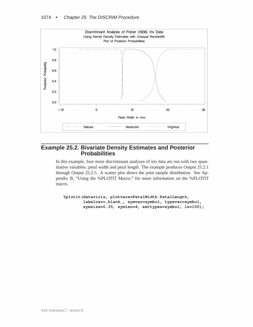
1074 � Chapter 25. The DISCRIM Procedure
Example 25.2. Bivariate Density Estimates and PosteriorProbabilities
In this example, four more discriminant analyses of iris data are run with two quan-titative variables: petal width and petal length. The example produces Output 25.2.1through Output 25.2.5. A scatter plot shows the joint sample distribution. See Ap-pendix B, “Using the %PLOTIT Macro,” for more information on the %PLOTITmacro.
%plotit(data=iris, plotvars=PetalWidth PetalLength,labelvar=_blank_, symvar=symbol, typevar=symbol,symsize=0.35, symlen=4, exttypes=symbol, ls=100);
SAS OnlineDoc: Version 8
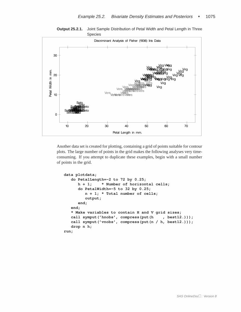
Example 25.2. Bivariate Density Estimates and Posteriors � 1075
Output 25.2.1. Joint Sample Distribution of Petal Width and Petal Length in ThreeSpecies
Another data set is created for plotting, containing a grid of points suitable for contourplots. The large number of points in the grid makes the following analyses very time-consuming. If you attempt to duplicate these examples, begin with a small numberof points in the grid.
data plotdata;do PetalLength=-2 to 72 by 0.25;
h + 1; * Number of horizontal cells;do PetalWidth=-5 to 32 by 0.25;
n + 1; * Total number of cells;output;
end;end;* Make variables to contain H and V grid sizes;call symput(’hnobs’, compress(put(h , best12.)));call symput(’vnobs’, compress(put(n / h, best12.)));drop n h;
run;
SAS OnlineDoc: Version 8
1076 � Chapter 25. The DISCRIM Procedure
A macro CONTOUR is defined to make contour plots of density estimates and pos-terior probabilities. Classification results are also plotted on the same grid.
%macro contour;data contour(keep=PetalWidth PetalLength symbol density);
set plotd(in=d) iris;if d then density = max(setosa,versicolor,virginica);
run;
title3 ’Plot of Estimated Densities’;%plotit(data=contour, plotvars=PetalWidth PetalLength,
labelvar=_blank_, symvar=symbol, typevar=symbol,symlen=4, exttypes=symbol contour, ls=100,paint=density white black, rgbtypes=contour,hnobs=&hnobs, vnobs=&vnobs, excolors=white,rgbround=-16 1 1 1, extend=close, options=noclip,types =Setosa Versicolor Virginica ’’,symtype=symbol symbol symbol contour,symsize=0.6 0.6 0.6 1,symfont=swiss swiss swiss solid)
data posterior(keep=PetalWidth PetalLength symbolprob _into_);
set plotp(in=d) iris;if d then prob = max(setosa,versicolor,virginica);
run;
title3 ’Plot of Posterior Probabilities ’’(Black to White is Low to High Probability)’;
%plotit(data=posterior, plotvars=PetalWidth PetalLength,labelvar=_blank_, symvar=symbol, typevar=symbol,symlen=4, exttypes=symbol contour, ls=100,paint=prob black white 0.3 0.999, rgbtypes=contour,hnobs=&hnobs, vnobs=&vnobs, excolors=white,rgbround=-16 1 1 1, extend=close, options=noclip,types =Setosa Versicolor Virginica ’’,symtype=symbol symbol symbol contour,symsize=0.6 0.6 0.6 1,symfont=swiss swiss swiss solid)
title3 ’Plot of Classification Results’;%plotit(data=posterior, plotvars=PetalWidth PetalLength,
labelvar=_blank_, symvar=symbol, typevar=symbol,symlen=4, exttypes=symbol contour, ls=100,paint=_into_ CXCCCCCC CXDDDDDD white,
rgbtypes=contour, hnobs=&hnobs, vnobs=&vnobs,excolors=white,
extend=close, options=noclip,types =Setosa Versicolor Virginica ’’,symtype=symbol symbol symbol contour,symsize=0.6 0.6 0.6 1,symfont=swiss swiss swiss solid)
%mend;
SAS OnlineDoc: Version 8
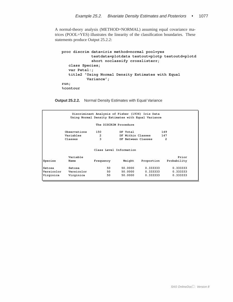
Example 25.2. Bivariate Density Estimates and Posteriors � 1077
A normal-theory analysis (METHOD=NORMAL) assuming equal covariance ma-trices (POOL=YES) illustrates the linearity of the classification boundaries. Thesestatements produce Output 25.2.2:
proc discrim data=iris method=normal pool=yestestdata=plotdata testout=plotp testoutd=plotdshort noclassify crosslisterr;
class Species;var Petal:;title2 ’Using Normal Density Estimates with Equal
Variance’;run;%contour
Output 25.2.2. Normal Density Estimates with Equal Variance
Discriminant Analysis of Fisher (1936) Iris DataUsing Normal Density Estimates with Equal Variance
The DISCRIM Procedure
Observations 150 DF Total 149Variables 2 DF Within Classes 147Classes 3 DF Between Classes 2
Class Level Information
Variable PriorSpecies Name Frequency Weight Proportion Probability
Setosa Setosa 50 50.0000 0.333333 0.333333Versicolor Versicolor 50 50.0000 0.333333 0.333333Virginica Virginica 50 50.0000 0.333333 0.333333
SAS OnlineDoc: Version 8
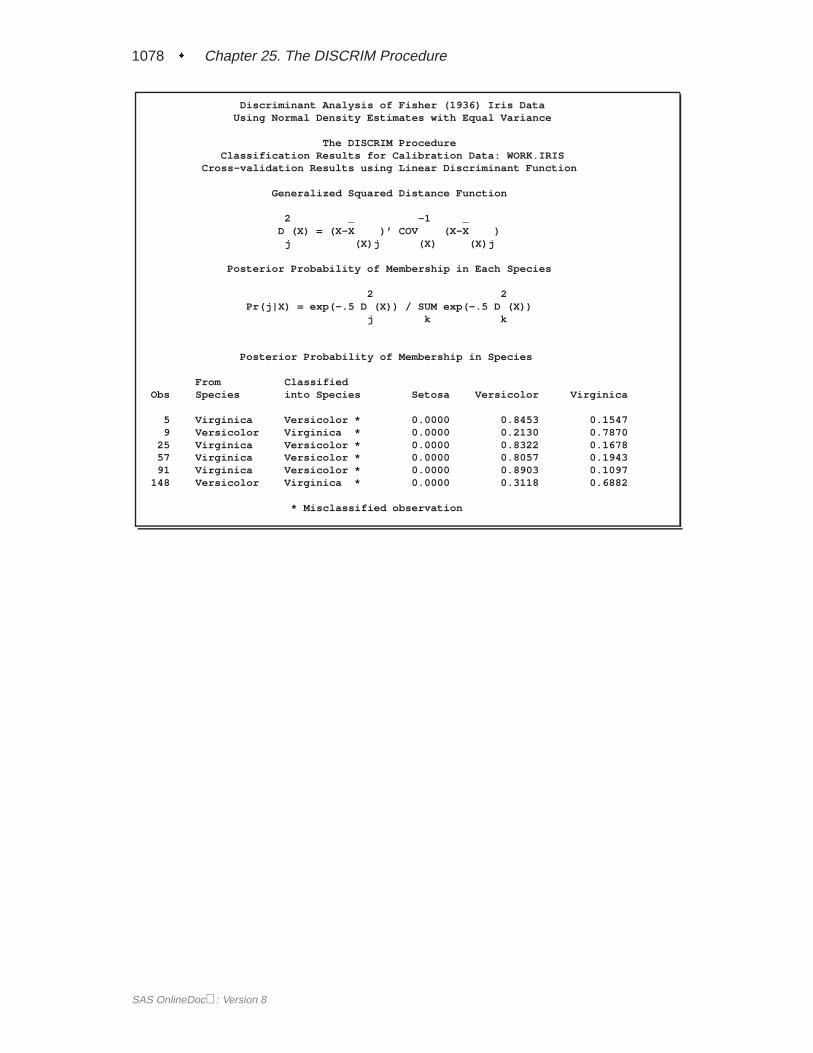
1078 � Chapter 25. The DISCRIM Procedure
Discriminant Analysis of Fisher (1936) Iris DataUsing Normal Density Estimates with Equal Variance
The DISCRIM ProcedureClassification Results for Calibration Data: WORK.IRIS
Cross-validation Results using Linear Discriminant Function
Generalized Squared Distance Function
2 _ -1 _D (X) = (X-X )’ COV (X-X )
j (X)j (X) (X)j
Posterior Probability of Membership in Each Species
2 2Pr(j|X) = exp(-.5 D (X)) / SUM exp(-.5 D (X))
j k k
Posterior Probability of Membership in Species
From ClassifiedObs Species into Species Setosa Versicolor Virginica
5 Virginica Versicolor * 0.0000 0.8453 0.15479 Versicolor Virginica * 0.0000 0.2130 0.7870
25 Virginica Versicolor * 0.0000 0.8322 0.167857 Virginica Versicolor * 0.0000 0.8057 0.194391 Virginica Versicolor * 0.0000 0.8903 0.1097
148 Versicolor Virginica * 0.0000 0.3118 0.6882
* Misclassified observation
SAS OnlineDoc: Version 8
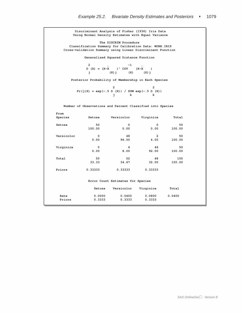
Example 25.2. Bivariate Density Estimates and Posteriors � 1079
Discriminant Analysis of Fisher (1936) Iris DataUsing Normal Density Estimates with Equal Variance
The DISCRIM ProcedureClassification Summary for Calibration Data: WORK.IRIS
Cross-validation Summary using Linear Discriminant Function
Generalized Squared Distance Function
2 _ -1 _D (X) = (X-X )’ COV (X-X )
j (X)j (X) (X)j
Posterior Probability of Membership in Each Species
2 2Pr(j|X) = exp(-.5 D (X)) / SUM exp(-.5 D (X))
j k k
Number of Observations and Percent Classified into Species
FromSpecies Setosa Versicolor Virginica Total
Setosa 50 0 0 50100.00 0.00 0.00 100.00
Versicolor 0 48 2 500.00 96.00 4.00 100.00
Virginica 0 4 46 500.00 8.00 92.00 100.00
Total 50 52 48 15033.33 34.67 32.00 100.00
Priors 0.33333 0.33333 0.33333
Error Count Estimates for Species
Setosa Versicolor Virginica Total
Rate 0.0000 0.0400 0.0800 0.0400Priors 0.3333 0.3333 0.3333
SAS OnlineDoc: Version 8
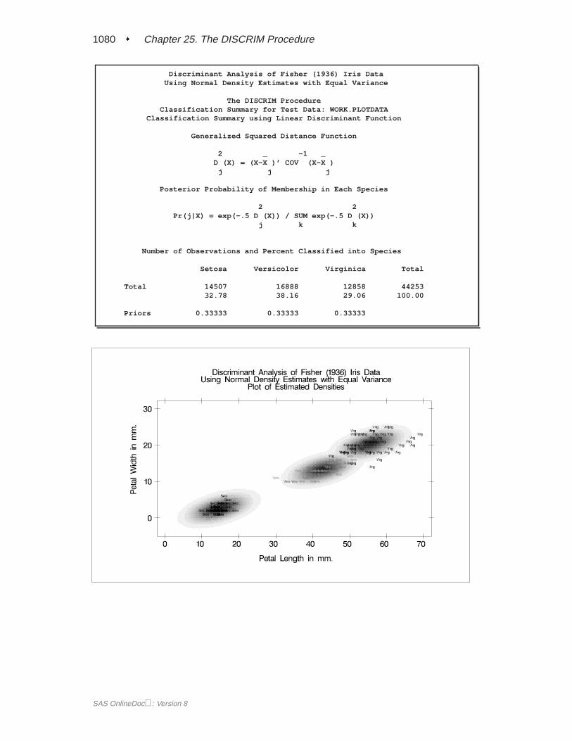
1080 � Chapter 25. The DISCRIM Procedure
Discriminant Analysis of Fisher (1936) Iris DataUsing Normal Density Estimates with Equal Variance
The DISCRIM ProcedureClassification Summary for Test Data: WORK.PLOTDATA
Classification Summary using Linear Discriminant Function
Generalized Squared Distance Function
2 _ -1 _D (X) = (X-X )’ COV (X-X )
j j j
Posterior Probability of Membership in Each Species
2 2Pr(j|X) = exp(-.5 D (X)) / SUM exp(-.5 D (X))
j k k
Number of Observations and Percent Classified into Species
Setosa Versicolor Virginica Total
Total 14507 16888 12858 4425332.78 38.16 29.06 100.00
Priors 0.33333 0.33333 0.33333
SAS OnlineDoc: Version 8
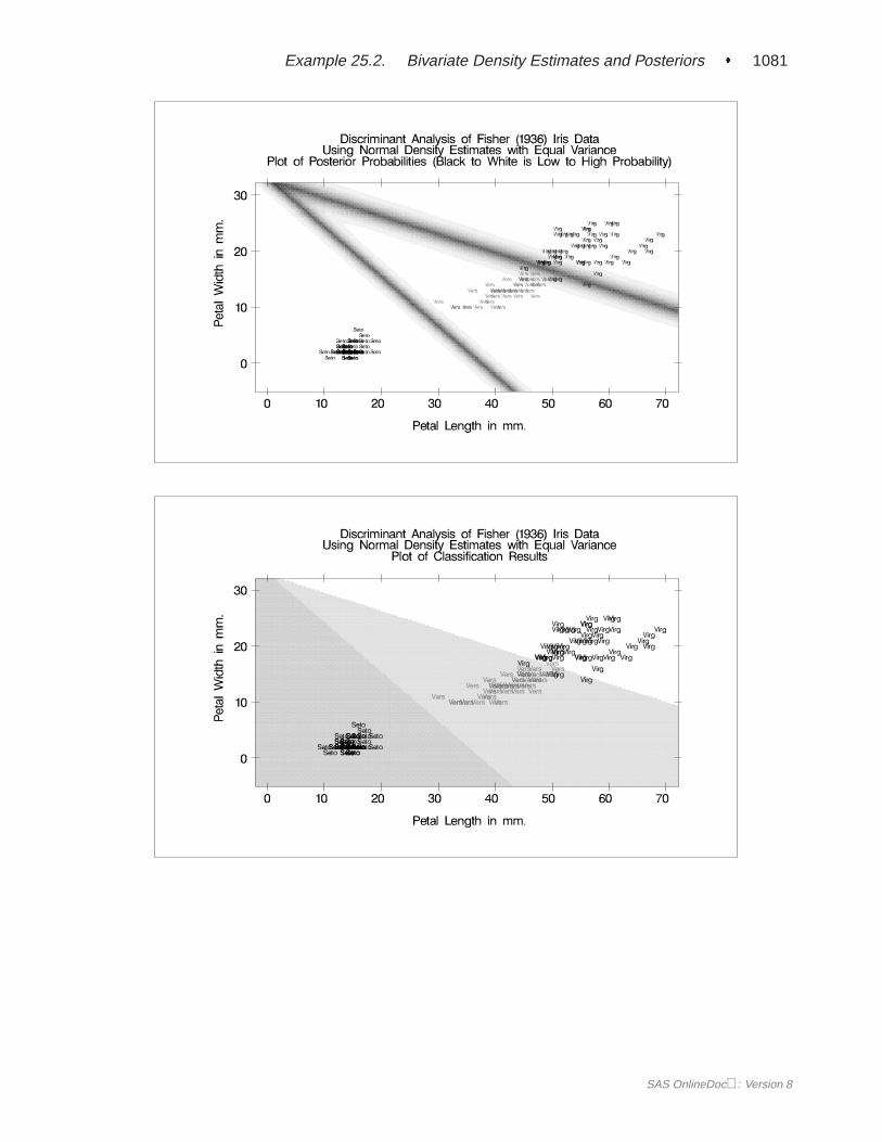
Example 25.2. Bivariate Density Estimates and Posteriors � 1081
SAS OnlineDoc: Version 8
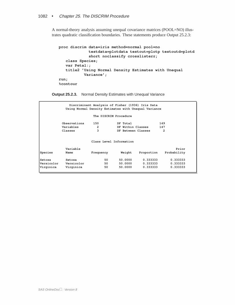
1082 � Chapter 25. The DISCRIM Procedure
A normal-theory analysis assuming unequal covariance matrices (POOL=NO) illus-trates quadratic classification boundaries. These statements produce Output 25.2.3:
proc discrim data=iris method=normal pool=notestdata=plotdata testout=plotp testoutd=plotdshort noclassify crosslisterr;
class Species;var Petal:;title2 ’Using Normal Density Estimates with Unequal
Variance’;run;%contour
Output 25.2.3. Normal Density Estimates with Unequal Variance
Discriminant Analysis of Fisher (1936) Iris DataUsing Normal Density Estimates with Unequal Variance
The DISCRIM Procedure
Observations 150 DF Total 149Variables 2 DF Within Classes 147Classes 3 DF Between Classes 2
Class Level Information
Variable PriorSpecies Name Frequency Weight Proportion Probability
Setosa Setosa 50 50.0000 0.333333 0.333333Versicolor Versicolor 50 50.0000 0.333333 0.333333Virginica Virginica 50 50.0000 0.333333 0.333333
SAS OnlineDoc: Version 8
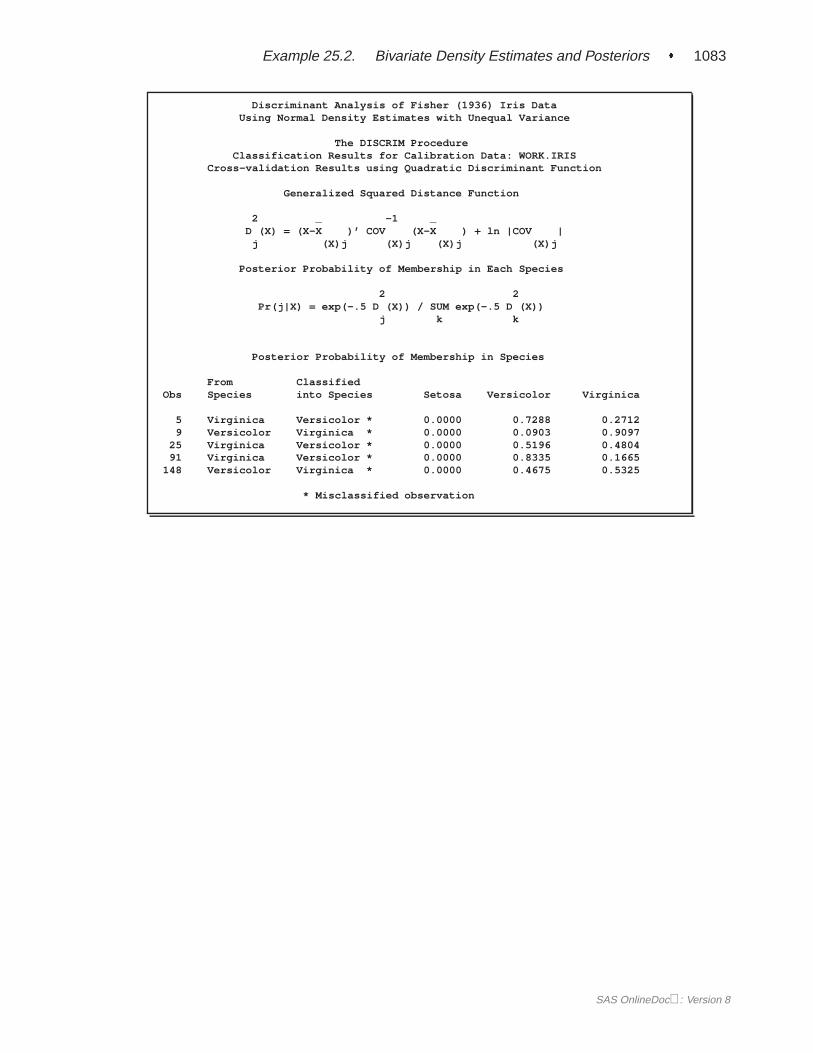
Example 25.2. Bivariate Density Estimates and Posteriors � 1083
Discriminant Analysis of Fisher (1936) Iris DataUsing Normal Density Estimates with Unequal Variance
The DISCRIM ProcedureClassification Results for Calibration Data: WORK.IRIS
Cross-validation Results using Quadratic Discriminant Function
Generalized Squared Distance Function
2 _ -1 _D (X) = (X-X )’ COV (X-X ) + ln |COV |
j (X)j (X)j (X)j (X)j
Posterior Probability of Membership in Each Species
2 2Pr(j|X) = exp(-.5 D (X)) / SUM exp(-.5 D (X))
j k k
Posterior Probability of Membership in Species
From ClassifiedObs Species into Species Setosa Versicolor Virginica
5 Virginica Versicolor * 0.0000 0.7288 0.27129 Versicolor Virginica * 0.0000 0.0903 0.9097
25 Virginica Versicolor * 0.0000 0.5196 0.480491 Virginica Versicolor * 0.0000 0.8335 0.1665
148 Versicolor Virginica * 0.0000 0.4675 0.5325
* Misclassified observation
SAS OnlineDoc: Version 8

1084 � Chapter 25. The DISCRIM Procedure
Discriminant Analysis of Fisher (1936) Iris DataUsing Normal Density Estimates with Unequal Variance
The DISCRIM ProcedureClassification Summary for Calibration Data: WORK.IRIS
Cross-validation Summary using Quadratic Discriminant Function
Generalized Squared Distance Function
2 _ -1 _D (X) = (X-X )’ COV (X-X ) + ln |COV |
j (X)j (X)j (X)j (X)j
Posterior Probability of Membership in Each Species
2 2Pr(j|X) = exp(-.5 D (X)) / SUM exp(-.5 D (X))
j k k
Number of Observations and Percent Classified into Species
FromSpecies Setosa Versicolor Virginica Total
Setosa 50 0 0 50100.00 0.00 0.00 100.00
Versicolor 0 48 2 500.00 96.00 4.00 100.00
Virginica 0 3 47 500.00 6.00 94.00 100.00
Total 50 51 49 15033.33 34.00 32.67 100.00
Priors 0.33333 0.33333 0.33333
Error Count Estimates for Species
Setosa Versicolor Virginica Total
Rate 0.0000 0.0400 0.0600 0.0333Priors 0.3333 0.3333 0.3333
SAS OnlineDoc: Version 8
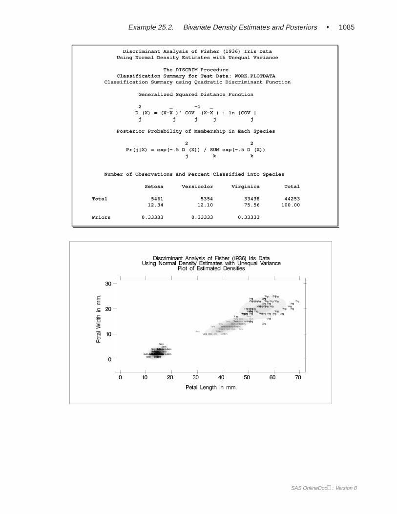
Example 25.2. Bivariate Density Estimates and Posteriors � 1085
Discriminant Analysis of Fisher (1936) Iris DataUsing Normal Density Estimates with Unequal Variance
The DISCRIM ProcedureClassification Summary for Test Data: WORK.PLOTDATA
Classification Summary using Quadratic Discriminant Function
Generalized Squared Distance Function
2 _ -1 _D (X) = (X-X )’ COV (X-X ) + ln |COV |
j j j j j
Posterior Probability of Membership in Each Species
2 2Pr(j|X) = exp(-.5 D (X)) / SUM exp(-.5 D (X))
j k k
Number of Observations and Percent Classified into Species
Setosa Versicolor Virginica Total
Total 5461 5354 33438 4425312.34 12.10 75.56 100.00
Priors 0.33333 0.33333 0.33333
SAS OnlineDoc: Version 8
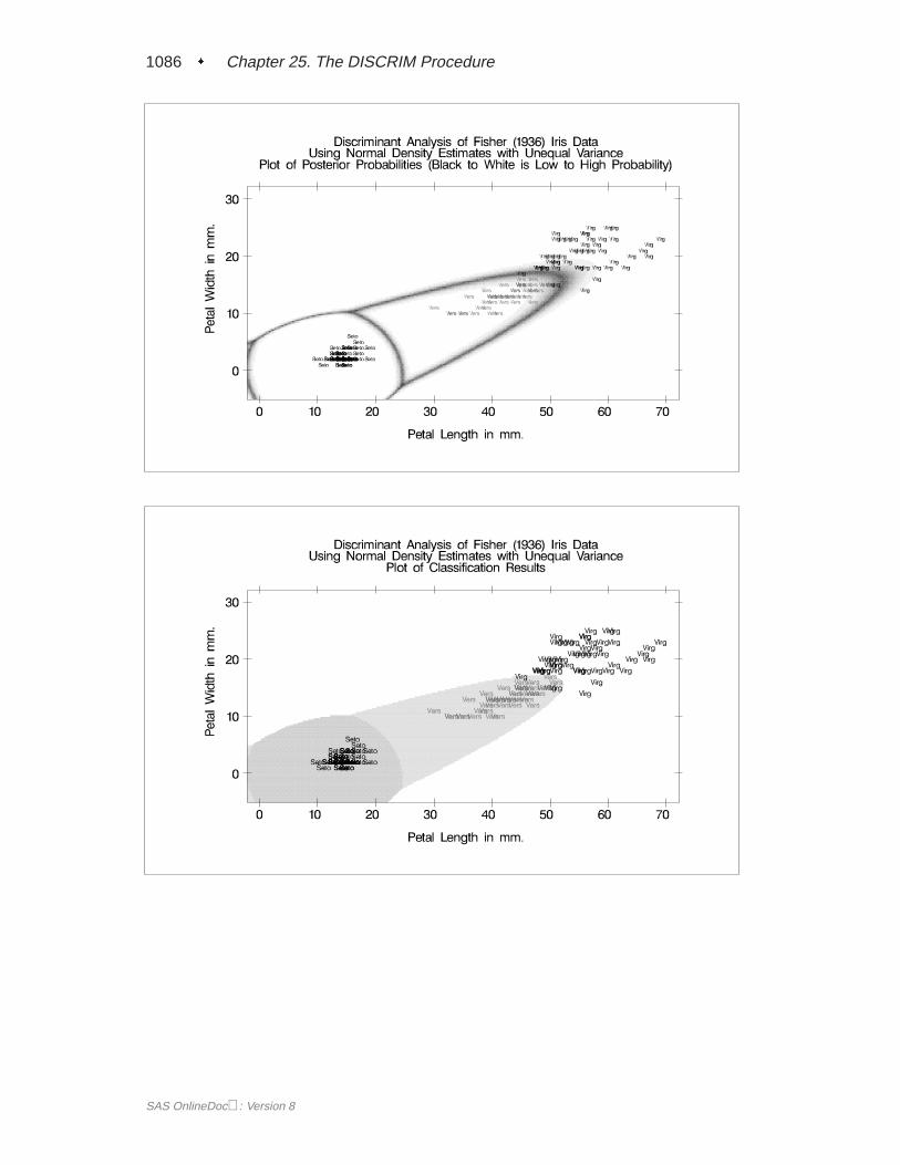
1086 � Chapter 25. The DISCRIM Procedure
SAS OnlineDoc: Version 8
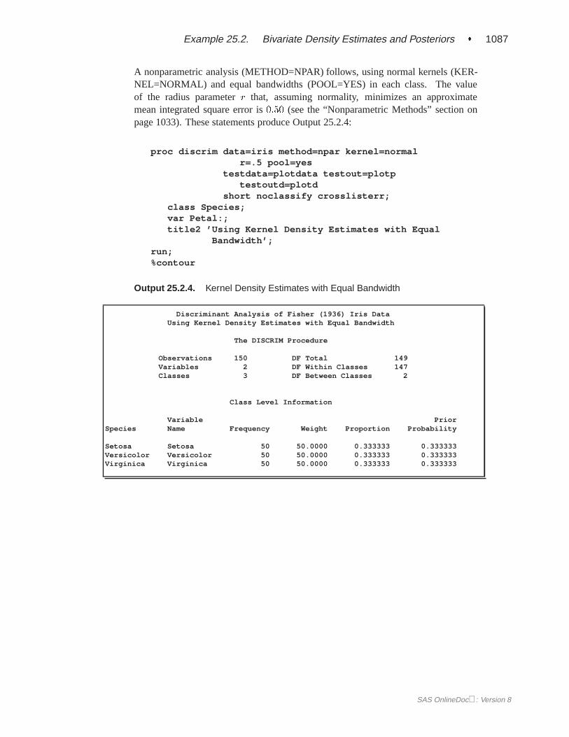
Example 25.2. Bivariate Density Estimates and Posteriors � 1087
A nonparametric analysis (METHOD=NPAR) follows, using normal kernels (KER-NEL=NORMAL) and equal bandwidths (POOL=YES) in each class. The valueof the radius parameterr that, assuming normality, minimizes an approximatemean integrated square error is0:50 (see the “Nonparametric Methods” section onpage 1033). These statements produce Output 25.2.4:
proc discrim data=iris method=npar kernel=normalr=.5 pool=yes
testdata=plotdata testout=plotptestoutd=plotd
short noclassify crosslisterr;class Species;var Petal:;title2 ’Using Kernel Density Estimates with Equal
Bandwidth’;run;%contour
Output 25.2.4. Kernel Density Estimates with Equal Bandwidth
Discriminant Analysis of Fisher (1936) Iris DataUsing Kernel Density Estimates with Equal Bandwidth
The DISCRIM Procedure
Observations 150 DF Total 149Variables 2 DF Within Classes 147Classes 3 DF Between Classes 2
Class Level Information
Variable PriorSpecies Name Frequency Weight Proportion Probability
Setosa Setosa 50 50.0000 0.333333 0.333333Versicolor Versicolor 50 50.0000 0.333333 0.333333Virginica Virginica 50 50.0000 0.333333 0.333333
SAS OnlineDoc: Version 8
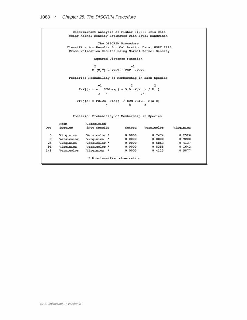
1088 � Chapter 25. The DISCRIM Procedure
Discriminant Analysis of Fisher (1936) Iris DataUsing Kernel Density Estimates with Equal Bandwidth
The DISCRIM ProcedureClassification Results for Calibration Data: WORK.IRIS
Cross-validation Results using Normal Kernel Density
Squared Distance Function
2 -1D (X,Y) = (X-Y)’ COV (X-Y)
Posterior Probability of Membership in Each Species
-1 2 2F(X|j) = n SUM exp( -.5 D (X,Y ) / R )
j i ji
Pr(j|X) = PRIOR F(X|j) / SUM PRIOR F(X|k)j k k
Posterior Probability of Membership in Species
From ClassifiedObs Species into Species Setosa Versicolor Virginica
5 Virginica Versicolor * 0.0000 0.7474 0.25269 Versicolor Virginica * 0.0000 0.0800 0.9200
25 Virginica Versicolor * 0.0000 0.5863 0.413791 Virginica Versicolor * 0.0000 0.8358 0.1642
148 Versicolor Virginica * 0.0000 0.4123 0.5877
* Misclassified observation
SAS OnlineDoc: Version 8
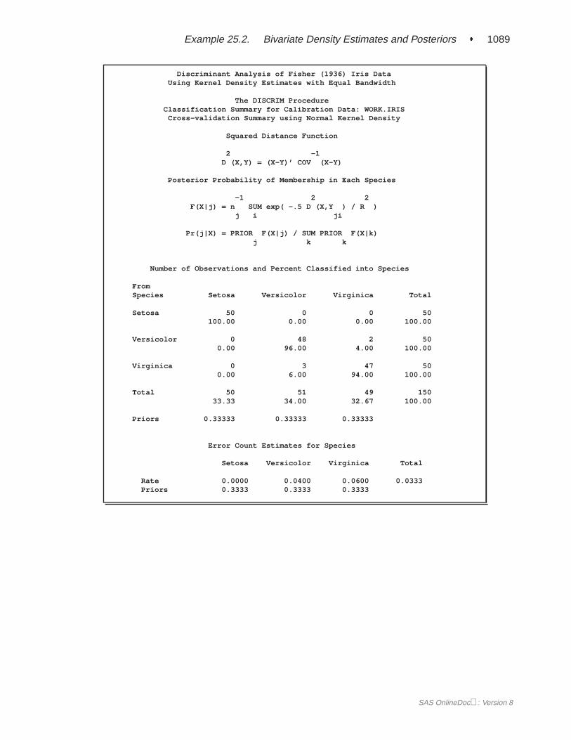
Example 25.2. Bivariate Density Estimates and Posteriors � 1089
Discriminant Analysis of Fisher (1936) Iris DataUsing Kernel Density Estimates with Equal Bandwidth
The DISCRIM ProcedureClassification Summary for Calibration Data: WORK.IRIS
Cross-validation Summary using Normal Kernel Density
Squared Distance Function
2 -1D (X,Y) = (X-Y)’ COV (X-Y)
Posterior Probability of Membership in Each Species
-1 2 2F(X|j) = n SUM exp( -.5 D (X,Y ) / R )
j i ji
Pr(j|X) = PRIOR F(X|j) / SUM PRIOR F(X|k)j k k
Number of Observations and Percent Classified into Species
FromSpecies Setosa Versicolor Virginica Total
Setosa 50 0 0 50100.00 0.00 0.00 100.00
Versicolor 0 48 2 500.00 96.00 4.00 100.00
Virginica 0 3 47 500.00 6.00 94.00 100.00
Total 50 51 49 15033.33 34.00 32.67 100.00
Priors 0.33333 0.33333 0.33333
Error Count Estimates for Species
Setosa Versicolor Virginica Total
Rate 0.0000 0.0400 0.0600 0.0333Priors 0.3333 0.3333 0.3333
SAS OnlineDoc: Version 8
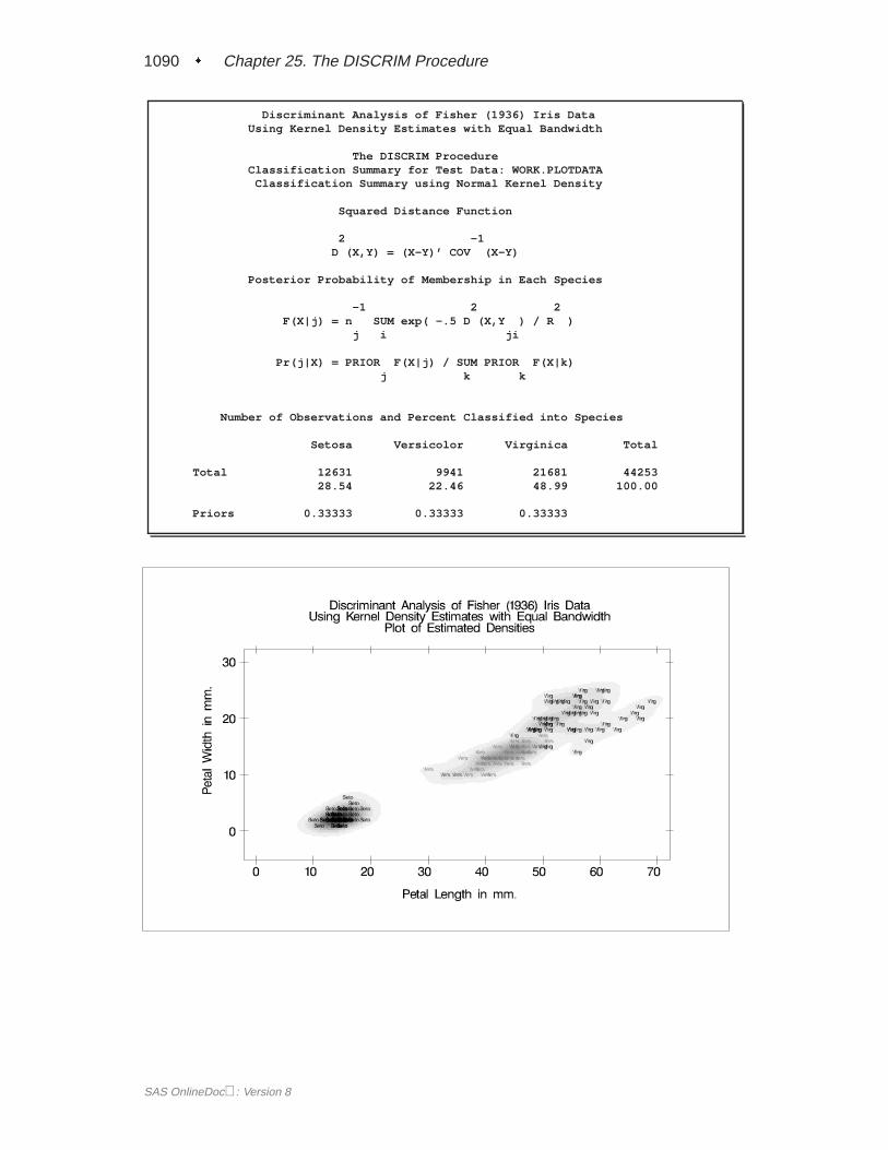
1090 � Chapter 25. The DISCRIM Procedure
Discriminant Analysis of Fisher (1936) Iris DataUsing Kernel Density Estimates with Equal Bandwidth
The DISCRIM ProcedureClassification Summary for Test Data: WORK.PLOTDATA
Classification Summary using Normal Kernel Density
Squared Distance Function
2 -1D (X,Y) = (X-Y)’ COV (X-Y)
Posterior Probability of Membership in Each Species
-1 2 2F(X|j) = n SUM exp( -.5 D (X,Y ) / R )
j i ji
Pr(j|X) = PRIOR F(X|j) / SUM PRIOR F(X|k)j k k
Number of Observations and Percent Classified into Species
Setosa Versicolor Virginica Total
Total 12631 9941 21681 4425328.54 22.46 48.99 100.00
Priors 0.33333 0.33333 0.33333
SAS OnlineDoc: Version 8
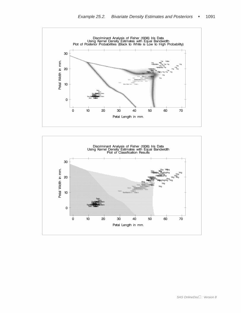
Example 25.2. Bivariate Density Estimates and Posteriors � 1091
SAS OnlineDoc: Version 8
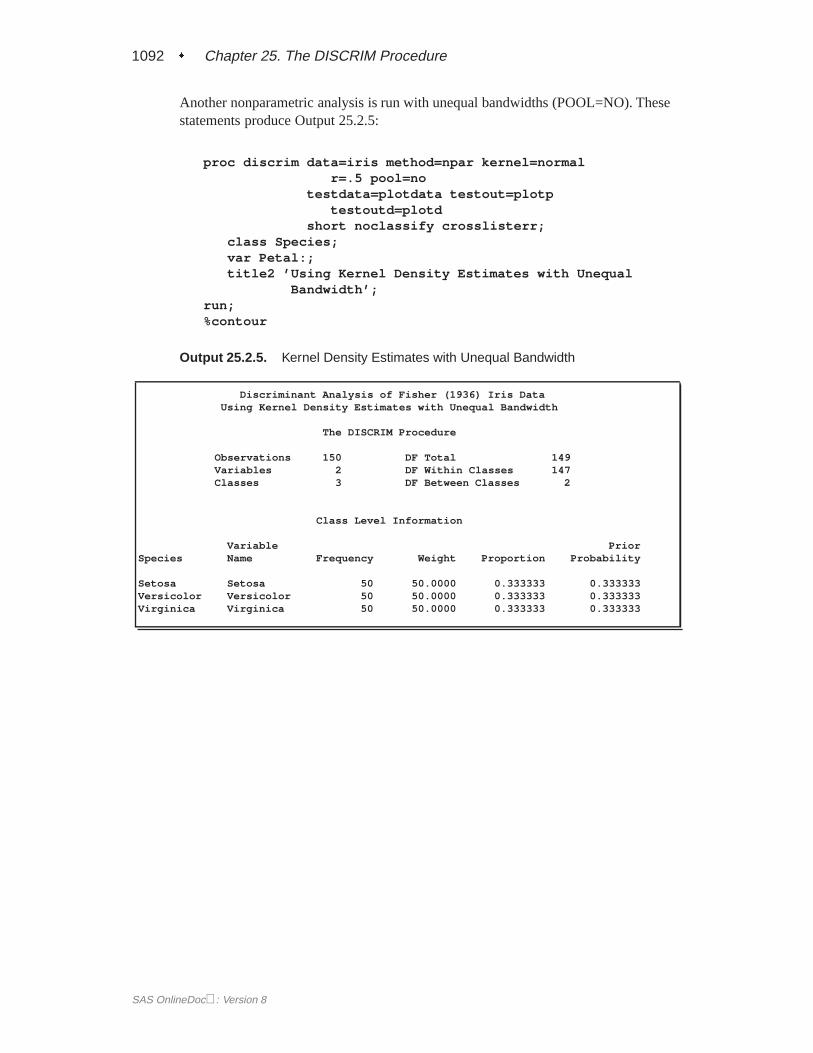
1092 � Chapter 25. The DISCRIM Procedure
Another nonparametric analysis is run with unequal bandwidths (POOL=NO). Thesestatements produce Output 25.2.5:
proc discrim data=iris method=npar kernel=normalr=.5 pool=no
testdata=plotdata testout=plotptestoutd=plotd
short noclassify crosslisterr;class Species;var Petal:;title2 ’Using Kernel Density Estimates with Unequal
Bandwidth’;run;%contour
Output 25.2.5. Kernel Density Estimates with Unequal Bandwidth
Discriminant Analysis of Fisher (1936) Iris DataUsing Kernel Density Estimates with Unequal Bandwidth
The DISCRIM Procedure
Observations 150 DF Total 149Variables 2 DF Within Classes 147Classes 3 DF Between Classes 2
Class Level Information
Variable PriorSpecies Name Frequency Weight Proportion Probability
Setosa Setosa 50 50.0000 0.333333 0.333333Versicolor Versicolor 50 50.0000 0.333333 0.333333Virginica Virginica 50 50.0000 0.333333 0.333333
SAS OnlineDoc: Version 8
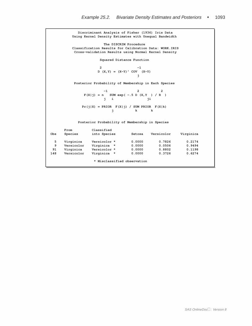
Example 25.2. Bivariate Density Estimates and Posteriors � 1093
Discriminant Analysis of Fisher (1936) Iris DataUsing Kernel Density Estimates with Unequal Bandwidth
The DISCRIM ProcedureClassification Results for Calibration Data: WORK.IRIS
Cross-validation Results using Normal Kernel Density
Squared Distance Function
2 -1D (X,Y) = (X-Y)’ COV (X-Y)
j
Posterior Probability of Membership in Each Species
-1 2 2F(X|j) = n SUM exp( -.5 D (X,Y ) / R )
j i ji
Pr(j|X) = PRIOR F(X|j) / SUM PRIOR F(X|k)j k k
Posterior Probability of Membership in Species
From ClassifiedObs Species into Species Setosa Versicolor Virginica
5 Virginica Versicolor * 0.0000 0.7826 0.21749 Versicolor Virginica * 0.0000 0.0506 0.9494
91 Virginica Versicolor * 0.0000 0.8802 0.1198148 Versicolor Virginica * 0.0000 0.3726 0.6274
* Misclassified observation
SAS OnlineDoc: Version 8
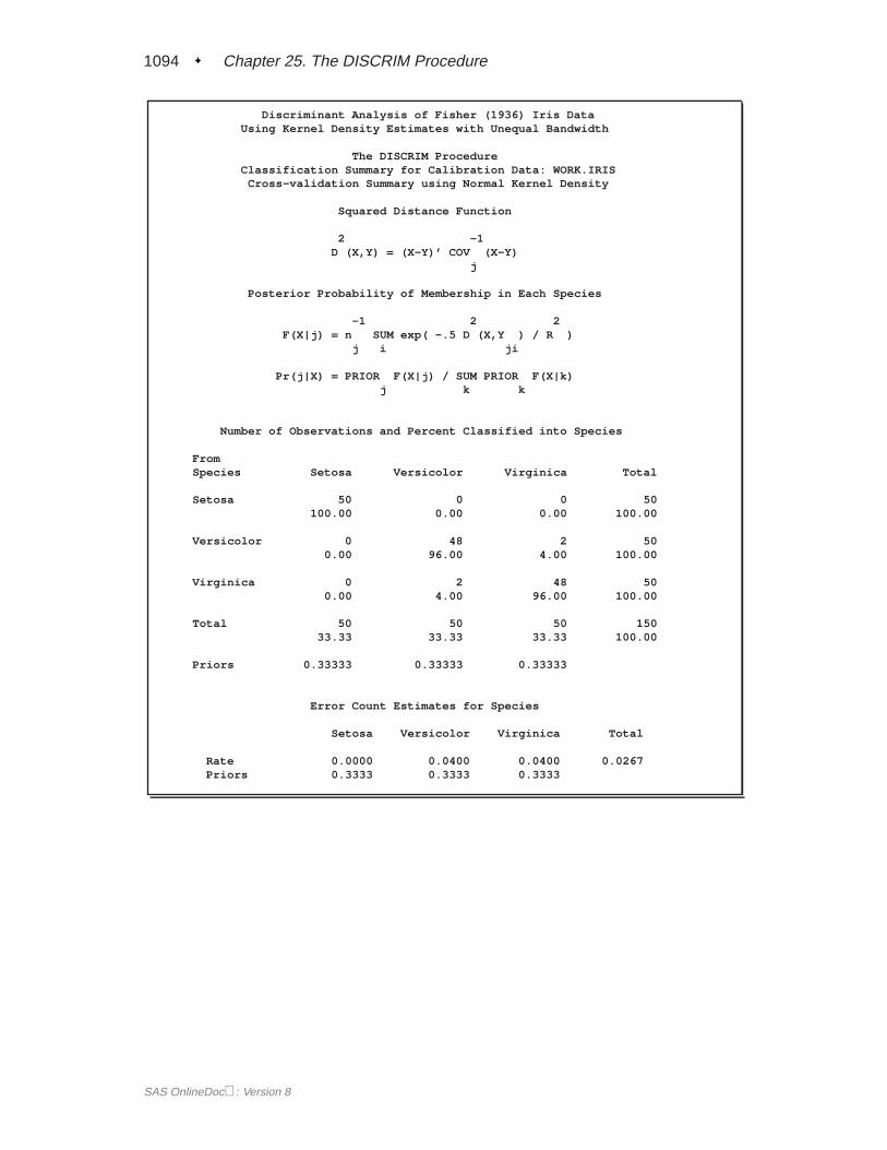
1094 � Chapter 25. The DISCRIM Procedure
Discriminant Analysis of Fisher (1936) Iris DataUsing Kernel Density Estimates with Unequal Bandwidth
The DISCRIM ProcedureClassification Summary for Calibration Data: WORK.IRIS
Cross-validation Summary using Normal Kernel Density
Squared Distance Function
2 -1D (X,Y) = (X-Y)’ COV (X-Y)
j
Posterior Probability of Membership in Each Species
-1 2 2F(X|j) = n SUM exp( -.5 D (X,Y ) / R )
j i ji
Pr(j|X) = PRIOR F(X|j) / SUM PRIOR F(X|k)j k k
Number of Observations and Percent Classified into Species
FromSpecies Setosa Versicolor Virginica Total
Setosa 50 0 0 50100.00 0.00 0.00 100.00
Versicolor 0 48 2 500.00 96.00 4.00 100.00
Virginica 0 2 48 500.00 4.00 96.00 100.00
Total 50 50 50 15033.33 33.33 33.33 100.00
Priors 0.33333 0.33333 0.33333
Error Count Estimates for Species
Setosa Versicolor Virginica Total
Rate 0.0000 0.0400 0.0400 0.0267Priors 0.3333 0.3333 0.3333
SAS OnlineDoc: Version 8
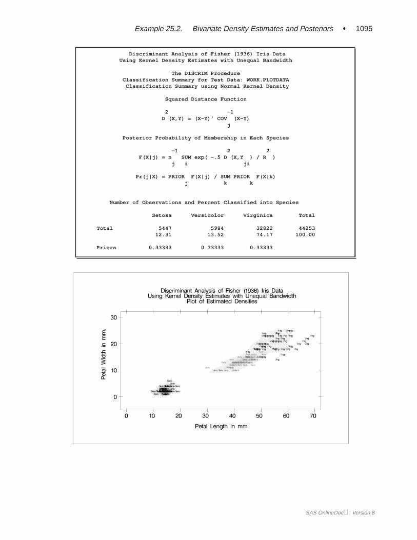
Example 25.2. Bivariate Density Estimates and Posteriors � 1095
Discriminant Analysis of Fisher (1936) Iris DataUsing Kernel Density Estimates with Unequal Bandwidth
The DISCRIM ProcedureClassification Summary for Test Data: WORK.PLOTDATA
Classification Summary using Normal Kernel Density
Squared Distance Function
2 -1D (X,Y) = (X-Y)’ COV (X-Y)
j
Posterior Probability of Membership in Each Species
-1 2 2F(X|j) = n SUM exp( -.5 D (X,Y ) / R )
j i ji
Pr(j|X) = PRIOR F(X|j) / SUM PRIOR F(X|k)j k k
Number of Observations and Percent Classified into Species
Setosa Versicolor Virginica Total
Total 5447 5984 32822 4425312.31 13.52 74.17 100.00
Priors 0.33333 0.33333 0.33333
SAS OnlineDoc: Version 8
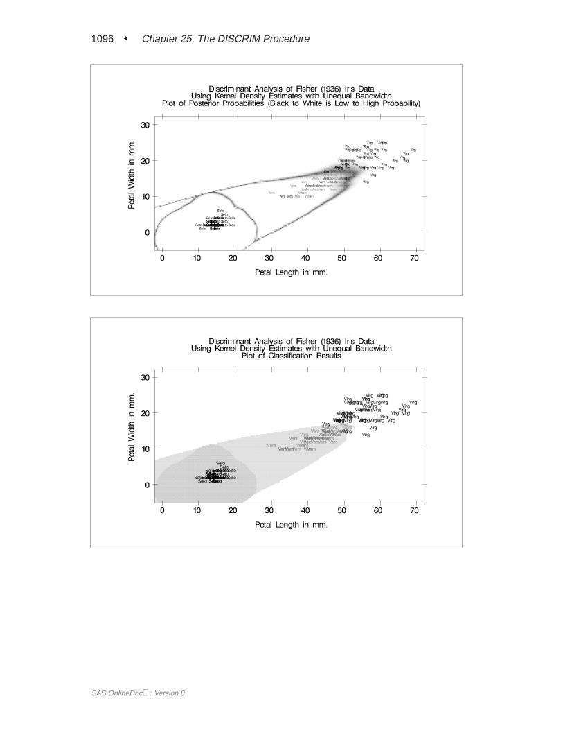
1096 � Chapter 25. The DISCRIM Procedure
SAS OnlineDoc: Version 8
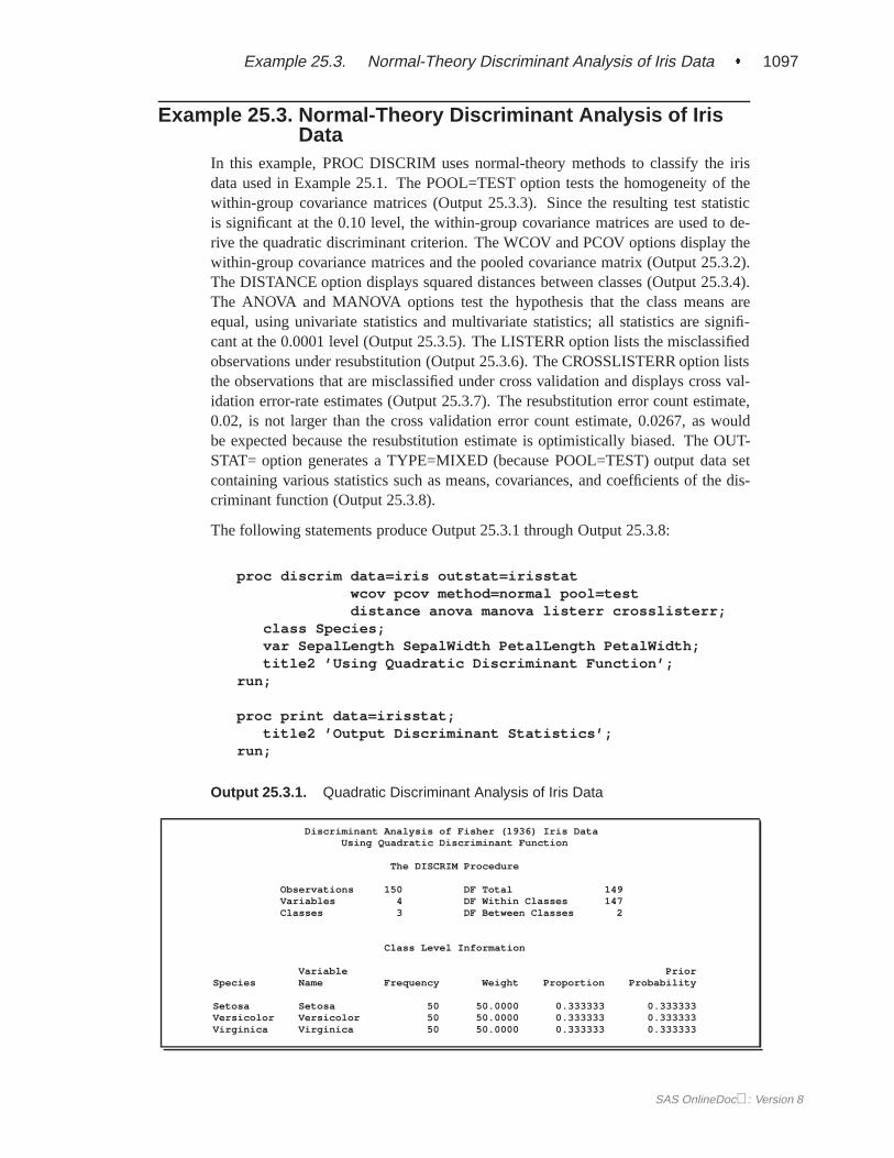
Example 25.3. Normal-Theory Discriminant Analysis of Iris Data � 1097
Example 25.3. Normal-Theory Discriminant Analysis of IrisData
In this example, PROC DISCRIM uses normal-theory methods to classify the irisdata used in Example 25.1. The POOL=TEST option tests the homogeneity of thewithin-group covariance matrices (Output 25.3.3). Since the resulting test statisticis significant at the 0.10 level, the within-group covariance matrices are used to de-rive the quadratic discriminant criterion. The WCOV and PCOV options display thewithin-group covariance matrices and the pooled covariance matrix (Output 25.3.2).The DISTANCE option displays squared distances between classes (Output 25.3.4).The ANOVA and MANOVA options test the hypothesis that the class means areequal, using univariate statistics and multivariate statistics; all statistics are signifi-cant at the 0.0001 level (Output 25.3.5). The LISTERR option lists the misclassifiedobservations under resubstitution (Output 25.3.6). The CROSSLISTERR option liststhe observations that are misclassified under cross validation and displays cross val-idation error-rate estimates (Output 25.3.7). The resubstitution error count estimate,0.02, is not larger than the cross validation error count estimate, 0.0267, as wouldbe expected because the resubstitution estimate is optimistically biased. The OUT-STAT= option generates a TYPE=MIXED (because POOL=TEST) output data setcontaining various statistics such as means, covariances, and coefficients of the dis-criminant function (Output 25.3.8).
The following statements produce Output 25.3.1 through Output 25.3.8:
proc discrim data=iris outstat=irisstatwcov pcov method=normal pool=testdistance anova manova listerr crosslisterr;
class Species;var SepalLength SepalWidth PetalLength PetalWidth;title2 ’Using Quadratic Discriminant Function’;
run;
proc print data=irisstat;title2 ’Output Discriminant Statistics’;
run;
Output 25.3.1. Quadratic Discriminant Analysis of Iris Data
Discriminant Analysis of Fisher (1936) Iris DataUsing Quadratic Discriminant Function
The DISCRIM Procedure
Observations 150 DF Total 149Variables 4 DF Within Classes 147Classes 3 DF Between Classes 2
Class Level Information
Variable PriorSpecies Name Frequency Weight Proportion Probability
Setosa Setosa 50 50.0000 0.333333 0.333333Versicolor Versicolor 50 50.0000 0.333333 0.333333Virginica Virginica 50 50.0000 0.333333 0.333333
SAS OnlineDoc: Version 8
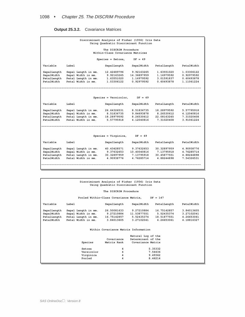
1098 � Chapter 25. The DISCRIM Procedure
Output 25.3.2. Covariance Matrices
Discriminant Analysis of Fisher (1936) Iris DataUsing Quadratic Discriminant Function
The DISCRIM ProcedureWithin-Class Covariance Matrices
Species = Setosa, DF = 49
Variable Label SepalLength SepalWidth PetalLength PetalWidth
SepalLength Sepal Length in mm. 12.42489796 9.92163265 1.63551020 1.03306122SepalWidth Sepal Width in mm. 9.92163265 14.36897959 1.16979592 0.92979592PetalLength Petal Length in mm. 1.63551020 1.16979592 3.01591837 0.60693878PetalWidth Petal Width in mm. 1.03306122 0.92979592 0.60693878 1.11061224
-----------------------------------------------------------------------------------------------
Species = Versicolor, DF = 49
Variable Label SepalLength SepalWidth PetalLength PetalWidth
SepalLength Sepal Length in mm. 26.64326531 8.51836735 18.28979592 5.57795918SepalWidth Sepal Width in mm. 8.51836735 9.84693878 8.26530612 4.12040816PetalLength Petal Length in mm. 18.28979592 8.26530612 22.08163265 7.31020408PetalWidth Petal Width in mm. 5.57795918 4.12040816 7.31020408 3.91061224
-----------------------------------------------------------------------------------------------
Species = Virginica, DF = 49
Variable Label SepalLength SepalWidth PetalLength PetalWidth
SepalLength Sepal Length in mm. 40.43428571 9.37632653 30.32897959 4.90938776SepalWidth Sepal Width in mm. 9.37632653 10.40040816 7.13795918 4.76285714PetalLength Petal Length in mm. 30.32897959 7.13795918 30.45877551 4.88244898PetalWidth Petal Width in mm. 4.90938776 4.76285714 4.88244898 7.54326531
-----------------------------------------------------------------------------------------------
Discriminant Analysis of Fisher (1936) Iris DataUsing Quadratic Discriminant Function
The DISCRIM Procedure
Pooled Within-Class Covariance Matrix, DF = 147
Variable Label SepalLength SepalWidth PetalLength PetalWidth
SepalLength Sepal Length in mm. 26.50081633 9.27210884 16.75142857 3.84013605SepalWidth Sepal Width in mm. 9.27210884 11.53877551 5.52435374 3.27102041PetalLength Petal Length in mm. 16.75142857 5.52435374 18.51877551 4.26653061PetalWidth Petal Width in mm. 3.84013605 3.27102041 4.26653061 4.18816327
Within Covariance Matrix Information
Natural Log of theCovariance Determinant of the
Species Matrix Rank Covariance Matrix
Setosa 4 5.35332Versicolor 4 7.54636Virginica 4 9.49362Pooled 4 8.46214
SAS OnlineDoc: Version 8
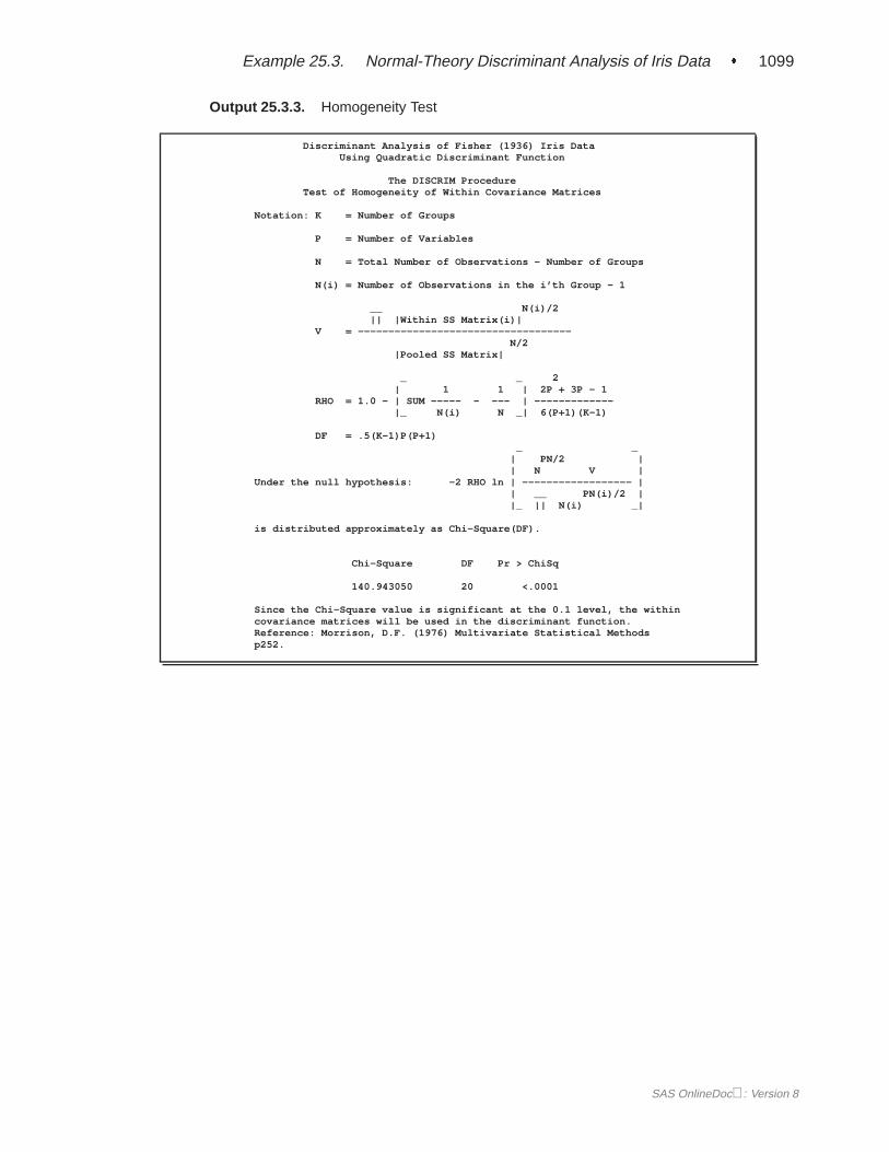
Example 25.3. Normal-Theory Discriminant Analysis of Iris Data � 1099
Output 25.3.3. Homogeneity Test
Discriminant Analysis of Fisher (1936) Iris DataUsing Quadratic Discriminant Function
The DISCRIM ProcedureTest of Homogeneity of Within Covariance Matrices
Notation: K = Number of Groups
P = Number of Variables
N = Total Number of Observations - Number of Groups
N(i) = Number of Observations in the i’th Group - 1
__ N(i)/2|| |Within SS Matrix(i)|
V = -----------------------------------N/2
|Pooled SS Matrix|
_ _ 2| 1 1 | 2P + 3P - 1
RHO = 1.0 - | SUM ----- - --- | -------------|_ N(i) N _| 6(P+1)(K-1)
DF = .5(K-1)P(P+1)_ _
| PN/2 || N V |
Under the null hypothesis: -2 RHO ln | ------------------ || __ PN(i)/2 ||_ || N(i) _|
is distributed approximately as Chi-Square(DF).
Chi-Square DF Pr > ChiSq
140.943050 20 <.0001
Since the Chi-Square value is significant at the 0.1 level, the withincovariance matrices will be used in the discriminant function.Reference: Morrison, D.F. (1976) Multivariate Statistical Methodsp252.
SAS OnlineDoc: Version 8
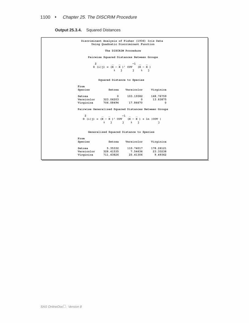
1100 � Chapter 25. The DISCRIM Procedure
Output 25.3.4. Squared Distances
Discriminant Analysis of Fisher (1936) Iris DataUsing Quadratic Discriminant Function
The DISCRIM Procedure
Pairwise Squared Distances Between Groups
2 _ _ -1 _ _D (i|j) = (X - X )’ COV (X - X )
i j j i j
Squared Distance to Species
FromSpecies Setosa Versicolor Virginica
Setosa 0 103.19382 168.76759Versicolor 323.06203 0 13.83875Virginica 706.08494 17.86670 0
Pairwise Generalized Squared Distances Between Groups
2 _ _ -1 _ _D (i|j) = (X - X )’ COV (X - X ) + ln |COV |
i j j i j j
Generalized Squared Distance to Species
FromSpecies Setosa Versicolor Virginica
Setosa 5.35332 110.74017 178.26121Versicolor 328.41535 7.54636 23.33238Virginica 711.43826 25.41306 9.49362
SAS OnlineDoc: Version 8
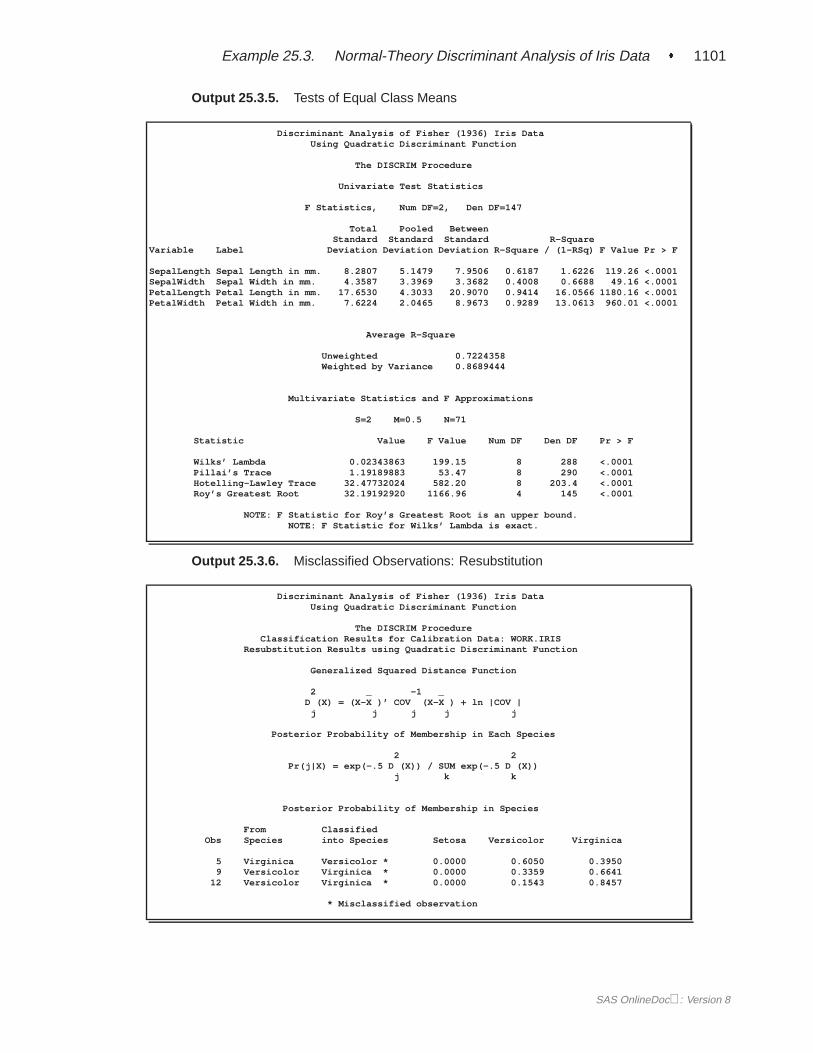
Example 25.3. Normal-Theory Discriminant Analysis of Iris Data � 1101
Output 25.3.5. Tests of Equal Class Means
Discriminant Analysis of Fisher (1936) Iris DataUsing Quadratic Discriminant Function
The DISCRIM Procedure
Univariate Test Statistics
F Statistics, Num DF=2, Den DF=147
Total Pooled BetweenStandard Standard Standard R-Square
Variable Label Deviation Deviation Deviation R-Square / (1-RSq) F Value Pr > F
SepalLength Sepal Length in mm. 8.2807 5.1479 7.9506 0.6187 1.6226 119.26 <.0001SepalWidth Sepal Width in mm. 4.3587 3.3969 3.3682 0.4008 0.6688 49.16 <.0001PetalLength Petal Length in mm. 17.6530 4.3033 20.9070 0.9414 16.0566 1180.16 <.0001PetalWidth Petal Width in mm. 7.6224 2.0465 8.9673 0.9289 13.0613 960.01 <.0001
Average R-Square
Unweighted 0.7224358Weighted by Variance 0.8689444
Multivariate Statistics and F Approximations
S=2 M=0.5 N=71
Statistic Value F Value Num DF Den DF Pr > F
Wilks’ Lambda 0.02343863 199.15 8 288 <.0001Pillai’s Trace 1.19189883 53.47 8 290 <.0001Hotelling-Lawley Trace 32.47732024 582.20 8 203.4 <.0001Roy’s Greatest Root 32.19192920 1166.96 4 145 <.0001
NOTE: F Statistic for Roy’s Greatest Root is an upper bound.NOTE: F Statistic for Wilks’ Lambda is exact.
Output 25.3.6. Misclassified Observations: Resubstitution
Discriminant Analysis of Fisher (1936) Iris DataUsing Quadratic Discriminant Function
The DISCRIM ProcedureClassification Results for Calibration Data: WORK.IRIS
Resubstitution Results using Quadratic Discriminant Function
Generalized Squared Distance Function
2 _ -1 _D (X) = (X-X )’ COV (X-X ) + ln |COV |
j j j j j
Posterior Probability of Membership in Each Species
2 2Pr(j|X) = exp(-.5 D (X)) / SUM exp(-.5 D (X))
j k k
Posterior Probability of Membership in Species
From ClassifiedObs Species into Species Setosa Versicolor Virginica
5 Virginica Versicolor * 0.0000 0.6050 0.39509 Versicolor Virginica * 0.0000 0.3359 0.6641
12 Versicolor Virginica * 0.0000 0.1543 0.8457
* Misclassified observation
SAS OnlineDoc: Version 8
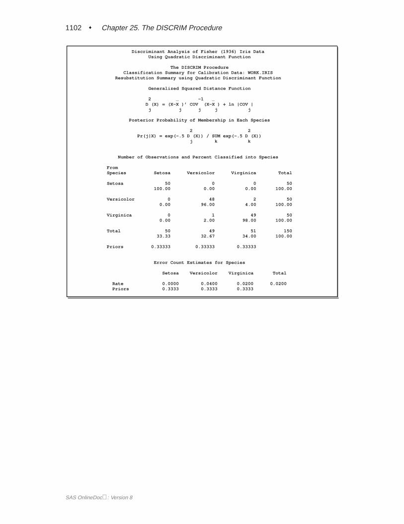
1102 � Chapter 25. The DISCRIM Procedure
Discriminant Analysis of Fisher (1936) Iris DataUsing Quadratic Discriminant Function
The DISCRIM ProcedureClassification Summary for Calibration Data: WORK.IRIS
Resubstitution Summary using Quadratic Discriminant Function
Generalized Squared Distance Function
2 _ -1 _D (X) = (X-X )’ COV (X-X ) + ln |COV |
j j j j j
Posterior Probability of Membership in Each Species
2 2Pr(j|X) = exp(-.5 D (X)) / SUM exp(-.5 D (X))
j k k
Number of Observations and Percent Classified into Species
FromSpecies Setosa Versicolor Virginica Total
Setosa 50 0 0 50100.00 0.00 0.00 100.00
Versicolor 0 48 2 500.00 96.00 4.00 100.00
Virginica 0 1 49 500.00 2.00 98.00 100.00
Total 50 49 51 15033.33 32.67 34.00 100.00
Priors 0.33333 0.33333 0.33333
Error Count Estimates for Species
Setosa Versicolor Virginica Total
Rate 0.0000 0.0400 0.0200 0.0200Priors 0.3333 0.3333 0.3333
SAS OnlineDoc: Version 8
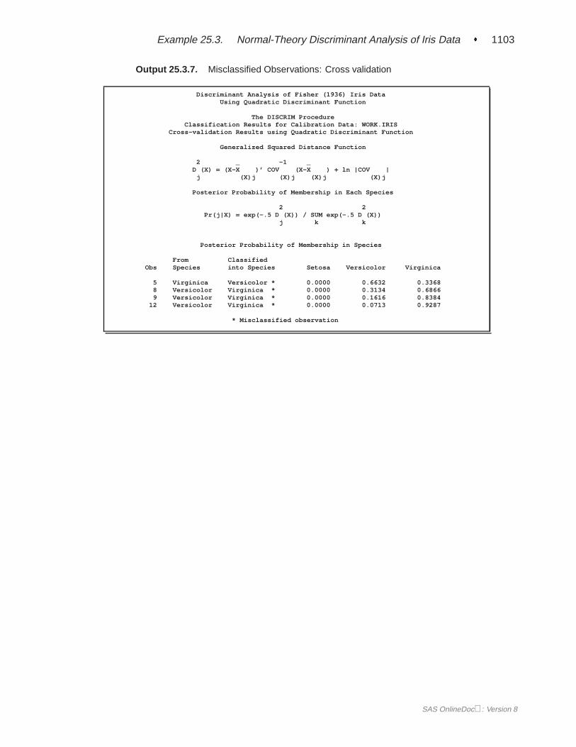
Example 25.3. Normal-Theory Discriminant Analysis of Iris Data � 1103
Output 25.3.7. Misclassified Observations: Cross validation
Discriminant Analysis of Fisher (1936) Iris DataUsing Quadratic Discriminant Function
The DISCRIM ProcedureClassification Results for Calibration Data: WORK.IRIS
Cross-validation Results using Quadratic Discriminant Function
Generalized Squared Distance Function
2 _ -1 _D (X) = (X-X )’ COV (X-X ) + ln |COV |
j (X)j (X)j (X)j (X)j
Posterior Probability of Membership in Each Species
2 2Pr(j|X) = exp(-.5 D (X)) / SUM exp(-.5 D (X))
j k k
Posterior Probability of Membership in Species
From ClassifiedObs Species into Species Setosa Versicolor Virginica
5 Virginica Versicolor * 0.0000 0.6632 0.33688 Versicolor Virginica * 0.0000 0.3134 0.68669 Versicolor Virginica * 0.0000 0.1616 0.8384
12 Versicolor Virginica * 0.0000 0.0713 0.9287
* Misclassified observation
SAS OnlineDoc: Version 8
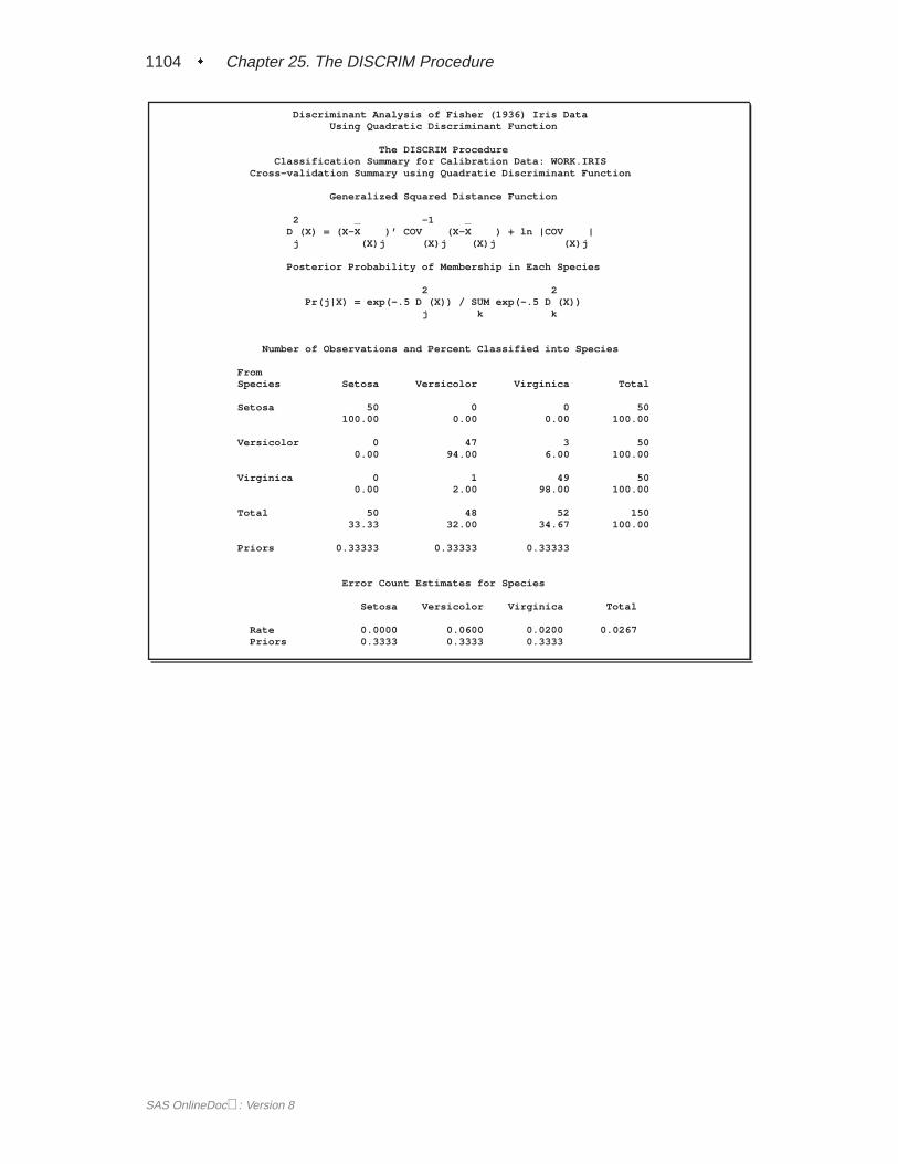
1104 � Chapter 25. The DISCRIM Procedure
Discriminant Analysis of Fisher (1936) Iris DataUsing Quadratic Discriminant Function
The DISCRIM ProcedureClassification Summary for Calibration Data: WORK.IRIS
Cross-validation Summary using Quadratic Discriminant Function
Generalized Squared Distance Function
2 _ -1 _D (X) = (X-X )’ COV (X-X ) + ln |COV |
j (X)j (X)j (X)j (X)j
Posterior Probability of Membership in Each Species
2 2Pr(j|X) = exp(-.5 D (X)) / SUM exp(-.5 D (X))
j k k
Number of Observations and Percent Classified into Species
FromSpecies Setosa Versicolor Virginica Total
Setosa 50 0 0 50100.00 0.00 0.00 100.00
Versicolor 0 47 3 500.00 94.00 6.00 100.00
Virginica 0 1 49 500.00 2.00 98.00 100.00
Total 50 48 52 15033.33 32.00 34.67 100.00
Priors 0.33333 0.33333 0.33333
Error Count Estimates for Species
Setosa Versicolor Virginica Total
Rate 0.0000 0.0600 0.0200 0.0267Priors 0.3333 0.3333 0.3333
SAS OnlineDoc: Version 8
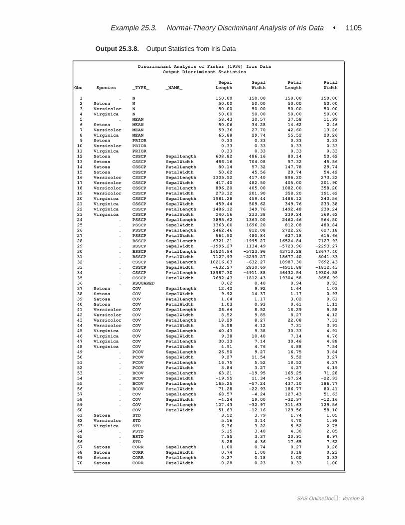
Example 25.3. Normal-Theory Discriminant Analysis of Iris Data � 1105
Output 25.3.8. Output Statistics from Iris Data
Discriminant Analysis of Fisher (1936) Iris DataOutput Discriminant Statistics
Sepal Sepal Petal PetalObs Species _TYPE_ _NAME_ Length Width Length Width
1 . N 150.00 150.00 150.00 150.002 Setosa N 50.00 50.00 50.00 50.003 Versicolor N 50.00 50.00 50.00 50.004 Virginica N 50.00 50.00 50.00 50.005 . MEAN 58.43 30.57 37.58 11.996 Setosa MEAN 50.06 34.28 14.62 2.467 Versicolor MEAN 59.36 27.70 42.60 13.268 Virginica MEAN 65.88 29.74 55.52 20.269 Setosa PRIOR 0.33 0.33 0.33 0.33
10 Versicolor PRIOR 0.33 0.33 0.33 0.3311 Virginica PRIOR 0.33 0.33 0.33 0.3312 Setosa CSSCP SepalLength 608.82 486.16 80.14 50.6213 Setosa CSSCP SepalWidth 486.16 704.08 57.32 45.5614 Setosa CSSCP PetalLength 80.14 57.32 147.78 29.7415 Setosa CSSCP PetalWidth 50.62 45.56 29.74 54.4216 Versicolor CSSCP SepalLength 1305.52 417.40 896.20 273.3217 Versicolor CSSCP SepalWidth 417.40 482.50 405.00 201.9018 Versicolor CSSCP PetalLength 896.20 405.00 1082.00 358.2019 Versicolor CSSCP PetalWidth 273.32 201.90 358.20 191.6220 Virginica CSSCP SepalLength 1981.28 459.44 1486.12 240.5621 Virginica CSSCP SepalWidth 459.44 509.62 349.76 233.3822 Virginica CSSCP PetalLength 1486.12 349.76 1492.48 239.2423 Virginica CSSCP PetalWidth 240.56 233.38 239.24 369.6224 . PSSCP SepalLength 3895.62 1363.00 2462.46 564.5025 . PSSCP SepalWidth 1363.00 1696.20 812.08 480.8426 . PSSCP PetalLength 2462.46 812.08 2722.26 627.1827 . PSSCP PetalWidth 564.50 480.84 627.18 615.6628 . BSSCP SepalLength 6321.21 -1995.27 16524.84 7127.9329 . BSSCP SepalWidth -1995.27 1134.49 -5723.96 -2293.2730 . BSSCP PetalLength 16524.84 -5723.96 43710.28 18677.4031 . BSSCP PetalWidth 7127.93 -2293.27 18677.40 8041.3332 . CSSCP SepalLength 10216.83 -632.27 18987.30 7692.4333 . CSSCP SepalWidth -632.27 2830.69 -4911.88 -1812.4334 . CSSCP PetalLength 18987.30 -4911.88 46432.54 19304.5835 . CSSCP PetalWidth 7692.43 -1812.43 19304.58 8656.9936 . RSQUARED 0.62 0.40 0.94 0.9337 Setosa COV SepalLength 12.42 9.92 1.64 1.0338 Setosa COV SepalWidth 9.92 14.37 1.17 0.9339 Setosa COV PetalLength 1.64 1.17 3.02 0.6140 Setosa COV PetalWidth 1.03 0.93 0.61 1.1141 Versicolor COV SepalLength 26.64 8.52 18.29 5.5842 Versicolor COV SepalWidth 8.52 9.85 8.27 4.1243 Versicolor COV PetalLength 18.29 8.27 22.08 7.3144 Versicolor COV PetalWidth 5.58 4.12 7.31 3.9145 Virginica COV SepalLength 40.43 9.38 30.33 4.9146 Virginica COV SepalWidth 9.38 10.40 7.14 4.7647 Virginica COV PetalLength 30.33 7.14 30.46 4.8848 Virginica COV PetalWidth 4.91 4.76 4.88 7.5449 . PCOV SepalLength 26.50 9.27 16.75 3.8450 . PCOV SepalWidth 9.27 11.54 5.52 3.2751 . PCOV PetalLength 16.75 5.52 18.52 4.2752 . PCOV PetalWidth 3.84 3.27 4.27 4.1953 . BCOV SepalLength 63.21 -19.95 165.25 71.2854 . BCOV SepalWidth -19.95 11.34 -57.24 -22.9355 . BCOV PetalLength 165.25 -57.24 437.10 186.7756 . BCOV PetalWidth 71.28 -22.93 186.77 80.4157 . COV SepalLength 68.57 -4.24 127.43 51.6358 . COV SepalWidth -4.24 19.00 -32.97 -12.1659 . COV PetalLength 127.43 -32.97 311.63 129.5660 . COV PetalWidth 51.63 -12.16 129.56 58.1061 Setosa STD 3.52 3.79 1.74 1.0562 Versicolor STD 5.16 3.14 4.70 1.9863 Virginica STD 6.36 3.22 5.52 2.7564 . PSTD 5.15 3.40 4.30 2.0565 . BSTD 7.95 3.37 20.91 8.9766 . STD 8.28 4.36 17.65 7.6267 Setosa CORR SepalLength 1.00 0.74 0.27 0.2868 Setosa CORR SepalWidth 0.74 1.00 0.18 0.2369 Setosa CORR PetalLength 0.27 0.18 1.00 0.3370 Setosa CORR PetalWidth 0.28 0.23 0.33 1.00
SAS OnlineDoc: Version 8
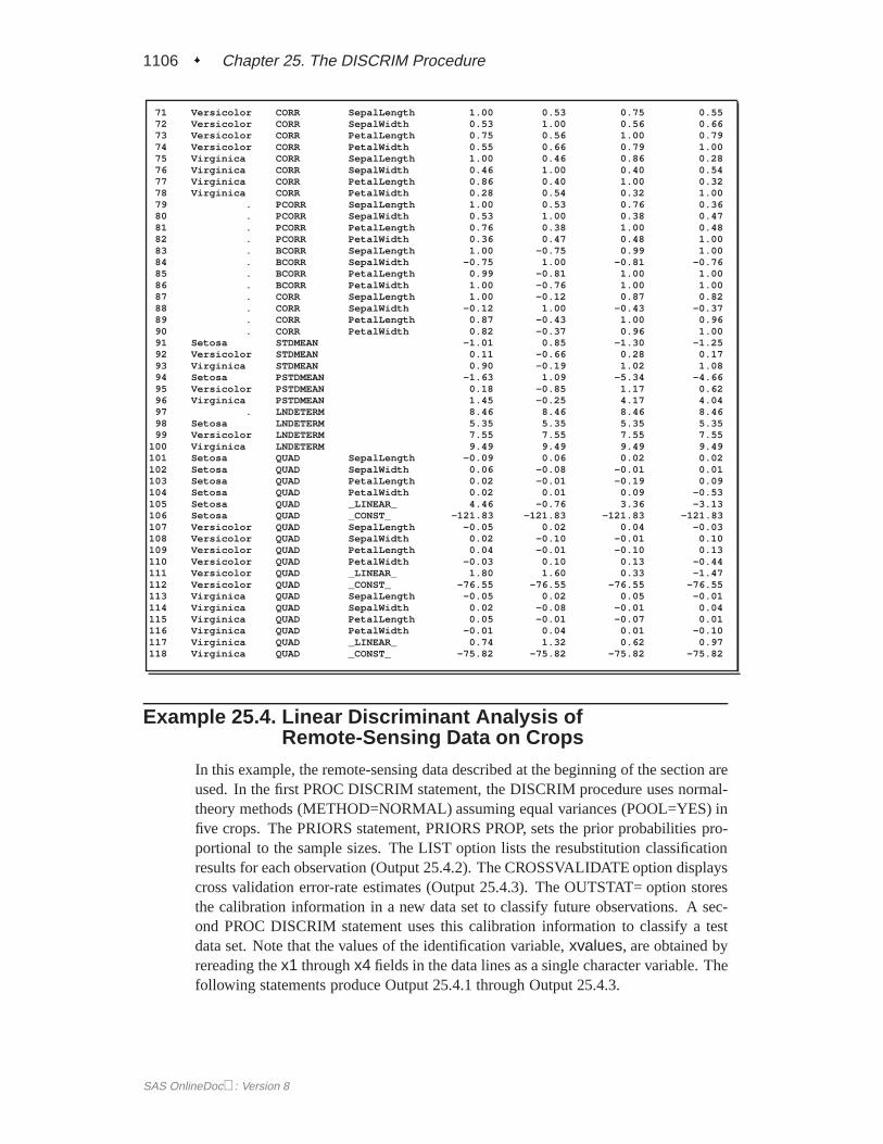
1106 � Chapter 25. The DISCRIM Procedure
71 Versicolor CORR SepalLength 1.00 0.53 0.75 0.5572 Versicolor CORR SepalWidth 0.53 1.00 0.56 0.6673 Versicolor CORR PetalLength 0.75 0.56 1.00 0.7974 Versicolor CORR PetalWidth 0.55 0.66 0.79 1.0075 Virginica CORR SepalLength 1.00 0.46 0.86 0.2876 Virginica CORR SepalWidth 0.46 1.00 0.40 0.5477 Virginica CORR PetalLength 0.86 0.40 1.00 0.3278 Virginica CORR PetalWidth 0.28 0.54 0.32 1.0079 . PCORR SepalLength 1.00 0.53 0.76 0.3680 . PCORR SepalWidth 0.53 1.00 0.38 0.4781 . PCORR PetalLength 0.76 0.38 1.00 0.4882 . PCORR PetalWidth 0.36 0.47 0.48 1.0083 . BCORR SepalLength 1.00 -0.75 0.99 1.0084 . BCORR SepalWidth -0.75 1.00 -0.81 -0.7685 . BCORR PetalLength 0.99 -0.81 1.00 1.0086 . BCORR PetalWidth 1.00 -0.76 1.00 1.0087 . CORR SepalLength 1.00 -0.12 0.87 0.8288 . CORR SepalWidth -0.12 1.00 -0.43 -0.3789 . CORR PetalLength 0.87 -0.43 1.00 0.9690 . CORR PetalWidth 0.82 -0.37 0.96 1.0091 Setosa STDMEAN -1.01 0.85 -1.30 -1.2592 Versicolor STDMEAN 0.11 -0.66 0.28 0.1793 Virginica STDMEAN 0.90 -0.19 1.02 1.0894 Setosa PSTDMEAN -1.63 1.09 -5.34 -4.6695 Versicolor PSTDMEAN 0.18 -0.85 1.17 0.6296 Virginica PSTDMEAN 1.45 -0.25 4.17 4.0497 . LNDETERM 8.46 8.46 8.46 8.4698 Setosa LNDETERM 5.35 5.35 5.35 5.3599 Versicolor LNDETERM 7.55 7.55 7.55 7.55
100 Virginica LNDETERM 9.49 9.49 9.49 9.49101 Setosa QUAD SepalLength -0.09 0.06 0.02 0.02102 Setosa QUAD SepalWidth 0.06 -0.08 -0.01 0.01103 Setosa QUAD PetalLength 0.02 -0.01 -0.19 0.09104 Setosa QUAD PetalWidth 0.02 0.01 0.09 -0.53105 Setosa QUAD _LINEAR_ 4.46 -0.76 3.36 -3.13106 Setosa QUAD _CONST_ -121.83 -121.83 -121.83 -121.83107 Versicolor QUAD SepalLength -0.05 0.02 0.04 -0.03108 Versicolor QUAD SepalWidth 0.02 -0.10 -0.01 0.10109 Versicolor QUAD PetalLength 0.04 -0.01 -0.10 0.13110 Versicolor QUAD PetalWidth -0.03 0.10 0.13 -0.44111 Versicolor QUAD _LINEAR_ 1.80 1.60 0.33 -1.47112 Versicolor QUAD _CONST_ -76.55 -76.55 -76.55 -76.55113 Virginica QUAD SepalLength -0.05 0.02 0.05 -0.01114 Virginica QUAD SepalWidth 0.02 -0.08 -0.01 0.04115 Virginica QUAD PetalLength 0.05 -0.01 -0.07 0.01116 Virginica QUAD PetalWidth -0.01 0.04 0.01 -0.10117 Virginica QUAD _LINEAR_ 0.74 1.32 0.62 0.97118 Virginica QUAD _CONST_ -75.82 -75.82 -75.82 -75.82
Example 25.4. Linear Discriminant Analysis ofRemote-Sensing Data on Crops
In this example, the remote-sensing data described at the beginning of the section areused. In the first PROC DISCRIM statement, the DISCRIM procedure uses normal-theory methods (METHOD=NORMAL) assuming equal variances (POOL=YES) infive crops. The PRIORS statement, PRIORS PROP, sets the prior probabilities pro-portional to the sample sizes. The LIST option lists the resubstitution classificationresults for each observation (Output 25.4.2). The CROSSVALIDATE option displayscross validation error-rate estimates (Output 25.4.3). The OUTSTAT= option storesthe calibration information in a new data set to classify future observations. A sec-ond PROC DISCRIM statement uses this calibration information to classify a testdata set. Note that the values of the identification variable,xvalues, are obtained byrereading thex1 throughx4 fields in the data lines as a single character variable. Thefollowing statements produce Output 25.4.1 through Output 25.4.3.
SAS OnlineDoc: Version 8
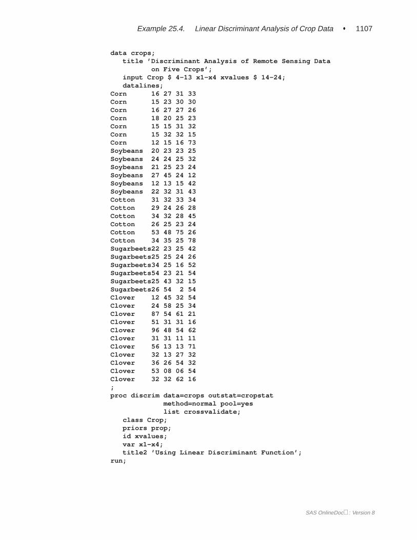
Example 25.4. Linear Discriminant Analysis of Crop Data � 1107
data crops;title ’Discriminant Analysis of Remote Sensing Data
on Five Crops’;input Crop $ 4-13 x1-x4 xvalues $ 14-24;datalines;
Corn 16 27 31 33Corn 15 23 30 30Corn 16 27 27 26Corn 18 20 25 23Corn 15 15 31 32Corn 15 32 32 15Corn 12 15 16 73Soybeans 20 23 23 25Soybeans 24 24 25 32Soybeans 21 25 23 24Soybeans 27 45 24 12Soybeans 12 13 15 42Soybeans 22 32 31 43Cotton 31 32 33 34Cotton 29 24 26 28Cotton 34 32 28 45Cotton 26 25 23 24Cotton 53 48 75 26Cotton 34 35 25 78Sugarbeets22 23 25 42Sugarbeets25 25 24 26Sugarbeets34 25 16 52Sugarbeets54 23 21 54Sugarbeets25 43 32 15Sugarbeets26 54 2 54Clover 12 45 32 54Clover 24 58 25 34Clover 87 54 61 21Clover 51 31 31 16Clover 96 48 54 62Clover 31 31 11 11Clover 56 13 13 71Clover 32 13 27 32Clover 36 26 54 32Clover 53 08 06 54Clover 32 32 62 16;proc discrim data=crops outstat=cropstat
method=normal pool=yeslist crossvalidate;
class Crop;priors prop;id xvalues;var x1-x4;title2 ’Using Linear Discriminant Function’;
run;
SAS OnlineDoc: Version 8
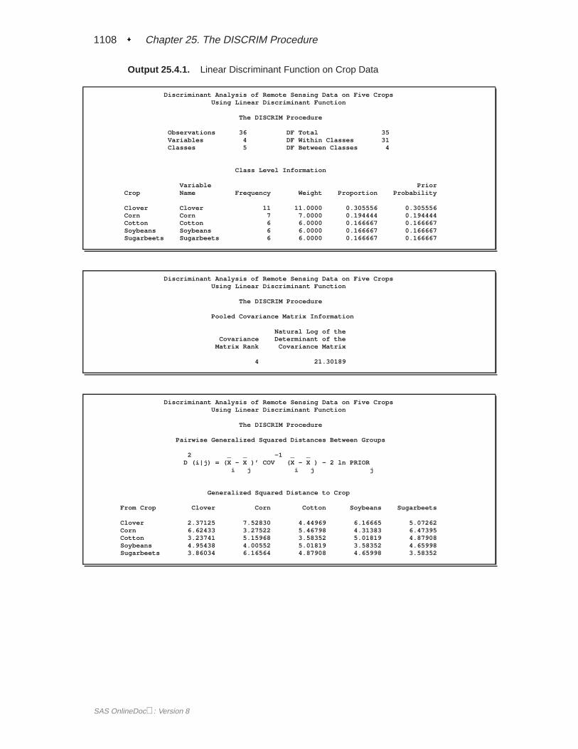
1108 � Chapter 25. The DISCRIM Procedure
Output 25.4.1. Linear Discriminant Function on Crop Data
Discriminant Analysis of Remote Sensing Data on Five CropsUsing Linear Discriminant Function
The DISCRIM Procedure
Observations 36 DF Total 35Variables 4 DF Within Classes 31Classes 5 DF Between Classes 4
Class Level Information
Variable PriorCrop Name Frequency Weight Proportion Probability
Clover Clover 11 11.0000 0.305556 0.305556Corn Corn 7 7.0000 0.194444 0.194444Cotton Cotton 6 6.0000 0.166667 0.166667Soybeans Soybeans 6 6.0000 0.166667 0.166667Sugarbeets Sugarbeets 6 6.0000 0.166667 0.166667
Discriminant Analysis of Remote Sensing Data on Five CropsUsing Linear Discriminant Function
The DISCRIM Procedure
Pooled Covariance Matrix Information
Natural Log of theCovariance Determinant of the
Matrix Rank Covariance Matrix
4 21.30189
Discriminant Analysis of Remote Sensing Data on Five CropsUsing Linear Discriminant Function
The DISCRIM Procedure
Pairwise Generalized Squared Distances Between Groups
2 _ _ -1 _ _D (i|j) = (X - X )’ COV (X - X ) - 2 ln PRIOR
i j i j j
Generalized Squared Distance to Crop
From Crop Clover Corn Cotton Soybeans Sugarbeets
Clover 2.37125 7.52830 4.44969 6.16665 5.07262Corn 6.62433 3.27522 5.46798 4.31383 6.47395Cotton 3.23741 5.15968 3.58352 5.01819 4.87908Soybeans 4.95438 4.00552 5.01819 3.58352 4.65998Sugarbeets 3.86034 6.16564 4.87908 4.65998 3.58352
SAS OnlineDoc: Version 8
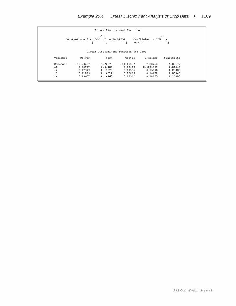
Example 25.4. Linear Discriminant Analysis of Crop Data � 1109
Linear Discriminant Function
_ -1 _ -1 _Constant = -.5 X’ COV X + ln PRIOR Coefficient = COV X
j j j Vector j
Linear Discriminant Function for Crop
Variable Clover Corn Cotton Soybeans Sugarbeets
Constant -10.98457 -7.72070 -11.46537 -7.28260 -9.80179x1 0.08907 -0.04180 0.02462 0.0000369 0.04245x2 0.17379 0.11970 0.17596 0.15896 0.20988x3 0.11899 0.16511 0.15880 0.10622 0.06540x4 0.15637 0.16768 0.18362 0.14133 0.16408
SAS OnlineDoc: Version 8
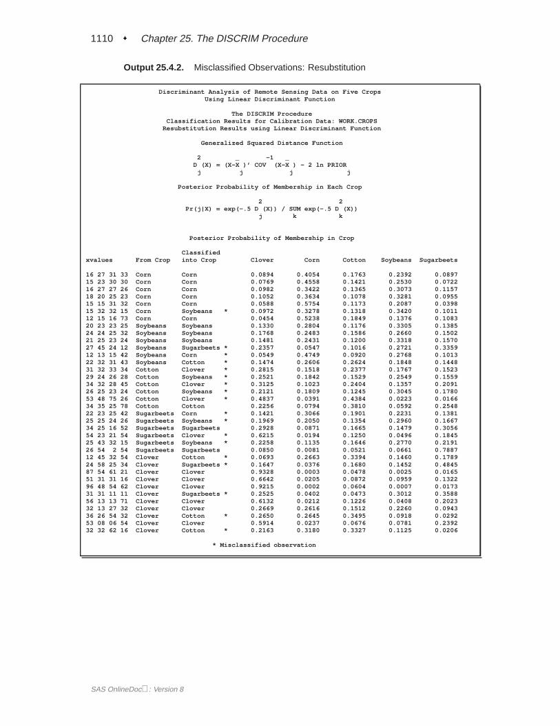
1110 � Chapter 25. The DISCRIM Procedure
Output 25.4.2. Misclassified Observations: Resubstitution
Discriminant Analysis of Remote Sensing Data on Five CropsUsing Linear Discriminant Function
The DISCRIM ProcedureClassification Results for Calibration Data: WORK.CROPS
Resubstitution Results using Linear Discriminant Function
Generalized Squared Distance Function
2 _ -1 _D (X) = (X-X )’ COV (X-X ) - 2 ln PRIOR
j j j j
Posterior Probability of Membership in Each Crop
2 2Pr(j|X) = exp(-.5 D (X)) / SUM exp(-.5 D (X))
j k k
Posterior Probability of Membership in Crop
Classifiedxvalues From Crop into Crop Clover Corn Cotton Soybeans Sugarbeets
16 27 31 33 Corn Corn 0.0894 0.4054 0.1763 0.2392 0.089715 23 30 30 Corn Corn 0.0769 0.4558 0.1421 0.2530 0.072216 27 27 26 Corn Corn 0.0982 0.3422 0.1365 0.3073 0.115718 20 25 23 Corn Corn 0.1052 0.3634 0.1078 0.3281 0.095515 15 31 32 Corn Corn 0.0588 0.5754 0.1173 0.2087 0.039815 32 32 15 Corn Soybeans * 0.0972 0.3278 0.1318 0.3420 0.101112 15 16 73 Corn Corn 0.0454 0.5238 0.1849 0.1376 0.108320 23 23 25 Soybeans Soybeans 0.1330 0.2804 0.1176 0.3305 0.138524 24 25 32 Soybeans Soybeans 0.1768 0.2483 0.1586 0.2660 0.150221 25 23 24 Soybeans Soybeans 0.1481 0.2431 0.1200 0.3318 0.157027 45 24 12 Soybeans Sugarbeets * 0.2357 0.0547 0.1016 0.2721 0.335912 13 15 42 Soybeans Corn * 0.0549 0.4749 0.0920 0.2768 0.101322 32 31 43 Soybeans Cotton * 0.1474 0.2606 0.2624 0.1848 0.144831 32 33 34 Cotton Clover * 0.2815 0.1518 0.2377 0.1767 0.152329 24 26 28 Cotton Soybeans * 0.2521 0.1842 0.1529 0.2549 0.155934 32 28 45 Cotton Clover * 0.3125 0.1023 0.2404 0.1357 0.209126 25 23 24 Cotton Soybeans * 0.2121 0.1809 0.1245 0.3045 0.178053 48 75 26 Cotton Clover * 0.4837 0.0391 0.4384 0.0223 0.016634 35 25 78 Cotton Cotton 0.2256 0.0794 0.3810 0.0592 0.254822 23 25 42 Sugarbeets Corn * 0.1421 0.3066 0.1901 0.2231 0.138125 25 24 26 Sugarbeets Soybeans * 0.1969 0.2050 0.1354 0.2960 0.166734 25 16 52 Sugarbeets Sugarbeets 0.2928 0.0871 0.1665 0.1479 0.305654 23 21 54 Sugarbeets Clover * 0.6215 0.0194 0.1250 0.0496 0.184525 43 32 15 Sugarbeets Soybeans * 0.2258 0.1135 0.1646 0.2770 0.219126 54 2 54 Sugarbeets Sugarbeets 0.0850 0.0081 0.0521 0.0661 0.788712 45 32 54 Clover Cotton * 0.0693 0.2663 0.3394 0.1460 0.178924 58 25 34 Clover Sugarbeets * 0.1647 0.0376 0.1680 0.1452 0.484587 54 61 21 Clover Clover 0.9328 0.0003 0.0478 0.0025 0.016551 31 31 16 Clover Clover 0.6642 0.0205 0.0872 0.0959 0.132296 48 54 62 Clover Clover 0.9215 0.0002 0.0604 0.0007 0.017331 31 11 11 Clover Sugarbeets * 0.2525 0.0402 0.0473 0.3012 0.358856 13 13 71 Clover Clover 0.6132 0.0212 0.1226 0.0408 0.202332 13 27 32 Clover Clover 0.2669 0.2616 0.1512 0.2260 0.094336 26 54 32 Clover Cotton * 0.2650 0.2645 0.3495 0.0918 0.029253 08 06 54 Clover Clover 0.5914 0.0237 0.0676 0.0781 0.239232 32 62 16 Clover Cotton * 0.2163 0.3180 0.3327 0.1125 0.0206
* Misclassified observation
SAS OnlineDoc: Version 8
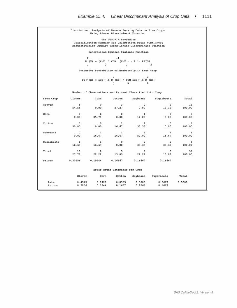
Example 25.4. Linear Discriminant Analysis of Crop Data � 1111
Discriminant Analysis of Remote Sensing Data on Five CropsUsing Linear Discriminant Function
The DISCRIM ProcedureClassification Summary for Calibration Data: WORK.CROPS
Resubstitution Summary using Linear Discriminant Function
Generalized Squared Distance Function
2 _ -1 _D (X) = (X-X )’ COV (X-X ) - 2 ln PRIOR
j j j j
Posterior Probability of Membership in Each Crop
2 2Pr(j|X) = exp(-.5 D (X)) / SUM exp(-.5 D (X))
j k k
Number of Observations and Percent Classified into Crop
From Crop Clover Corn Cotton Soybeans Sugarbeets Total
Clover 6 0 3 0 2 1154.55 0.00 27.27 0.00 18.18 100.00
Corn 0 6 0 1 0 70.00 85.71 0.00 14.29 0.00 100.00
Cotton 3 0 1 2 0 650.00 0.00 16.67 33.33 0.00 100.00
Soybeans 0 1 1 3 1 60.00 16.67 16.67 50.00 16.67 100.00
Sugarbeets 1 1 0 2 2 616.67 16.67 0.00 33.33 33.33 100.00
Total 10 8 5 8 5 3627.78 22.22 13.89 22.22 13.89 100.00
Priors 0.30556 0.19444 0.16667 0.16667 0.16667
Error Count Estimates for Crop
Clover Corn Cotton Soybeans Sugarbeets Total
Rate 0.4545 0.1429 0.8333 0.5000 0.6667 0.5000Priors 0.3056 0.1944 0.1667 0.1667 0.1667
SAS OnlineDoc: Version 8
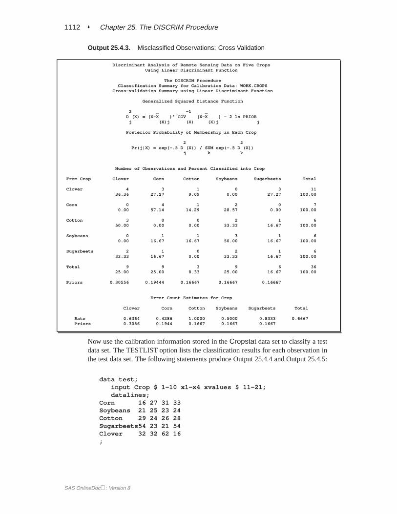
1112 � Chapter 25. The DISCRIM Procedure
Output 25.4.3. Misclassified Observations: Cross Validation
Discriminant Analysis of Remote Sensing Data on Five CropsUsing Linear Discriminant Function
The DISCRIM ProcedureClassification Summary for Calibration Data: WORK.CROPS
Cross-validation Summary using Linear Discriminant Function
Generalized Squared Distance Function
2 _ -1 _D (X) = (X-X )’ COV (X-X ) - 2 ln PRIOR
j (X)j (X) (X)j j
Posterior Probability of Membership in Each Crop
2 2Pr(j|X) = exp(-.5 D (X)) / SUM exp(-.5 D (X))
j k k
Number of Observations and Percent Classified into Crop
From Crop Clover Corn Cotton Soybeans Sugarbeets Total
Clover 4 3 1 0 3 1136.36 27.27 9.09 0.00 27.27 100.00
Corn 0 4 1 2 0 70.00 57.14 14.29 28.57 0.00 100.00
Cotton 3 0 0 2 1 650.00 0.00 0.00 33.33 16.67 100.00
Soybeans 0 1 1 3 1 60.00 16.67 16.67 50.00 16.67 100.00
Sugarbeets 2 1 0 2 1 633.33 16.67 0.00 33.33 16.67 100.00
Total 9 9 3 9 6 3625.00 25.00 8.33 25.00 16.67 100.00
Priors 0.30556 0.19444 0.16667 0.16667 0.16667
Error Count Estimates for Crop
Clover Corn Cotton Soybeans Sugarbeets Total
Rate 0.6364 0.4286 1.0000 0.5000 0.8333 0.6667Priors 0.3056 0.1944 0.1667 0.1667 0.1667
Now use the calibration information stored in theCropstat data set to classify a testdata set. The TESTLIST option lists the classification results for each observation inthe test data set. The following statements produce Output 25.4.4 and Output 25.4.5:
data test;input Crop $ 1-10 x1-x4 xvalues $ 11-21;datalines;
Corn 16 27 31 33Soybeans 21 25 23 24Cotton 29 24 26 28Sugarbeets54 23 21 54Clover 32 32 62 16;
SAS OnlineDoc: Version 8
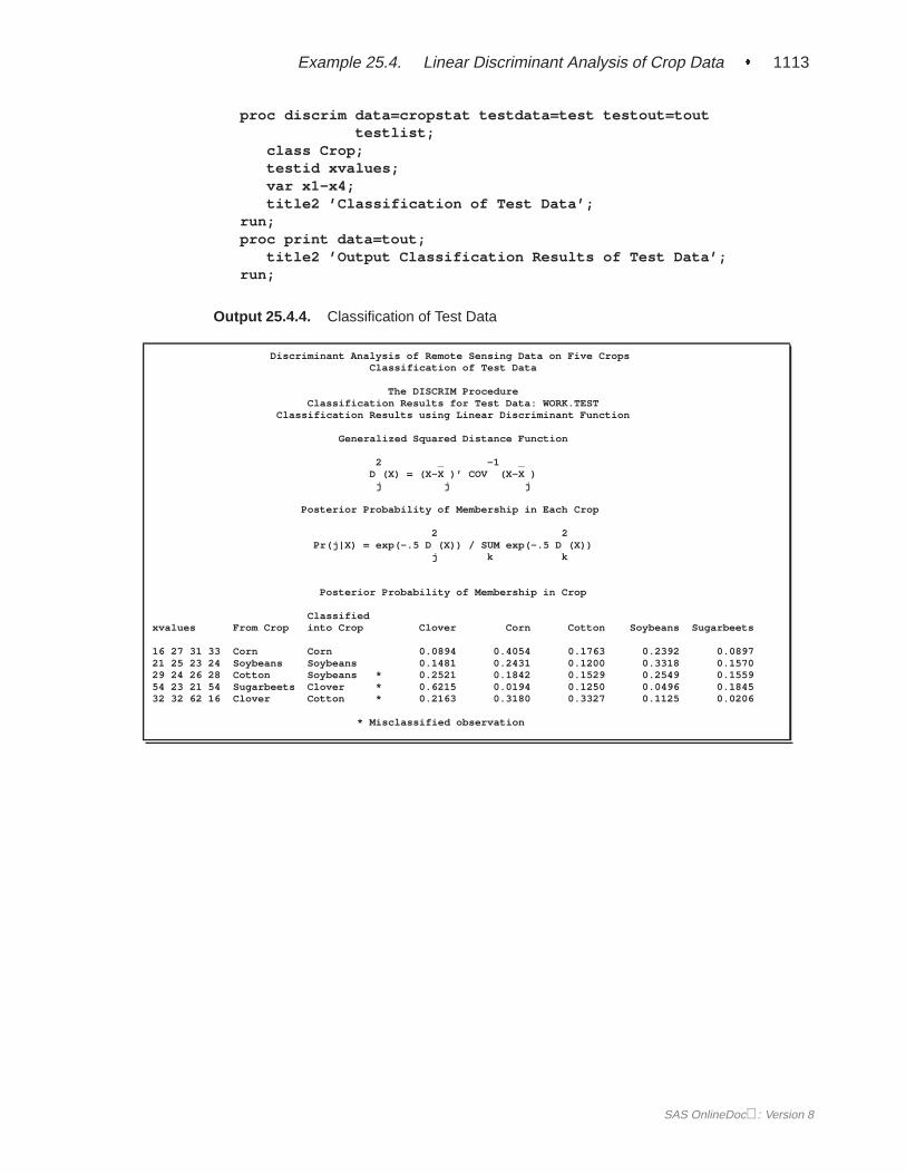
Example 25.4. Linear Discriminant Analysis of Crop Data � 1113
proc discrim data=cropstat testdata=test testout=touttestlist;
class Crop;testid xvalues;var x1-x4;title2 ’Classification of Test Data’;
run;proc print data=tout;
title2 ’Output Classification Results of Test Data’;run;
Output 25.4.4. Classification of Test Data
Discriminant Analysis of Remote Sensing Data on Five CropsClassification of Test Data
The DISCRIM ProcedureClassification Results for Test Data: WORK.TEST
Classification Results using Linear Discriminant Function
Generalized Squared Distance Function
2 _ -1 _D (X) = (X-X )’ COV (X-X )
j j j
Posterior Probability of Membership in Each Crop
2 2Pr(j|X) = exp(-.5 D (X)) / SUM exp(-.5 D (X))
j k k
Posterior Probability of Membership in Crop
Classifiedxvalues From Crop into Crop Clover Corn Cotton Soybeans Sugarbeets
16 27 31 33 Corn Corn 0.0894 0.4054 0.1763 0.2392 0.089721 25 23 24 Soybeans Soybeans 0.1481 0.2431 0.1200 0.3318 0.157029 24 26 28 Cotton Soybeans * 0.2521 0.1842 0.1529 0.2549 0.155954 23 21 54 Sugarbeets Clover * 0.6215 0.0194 0.1250 0.0496 0.184532 32 62 16 Clover Cotton * 0.2163 0.3180 0.3327 0.1125 0.0206
* Misclassified observation
SAS OnlineDoc: Version 8
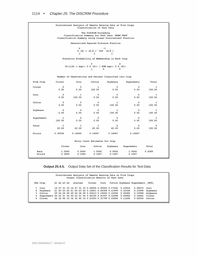
1114 � Chapter 25. The DISCRIM Procedure
Discriminant Analysis of Remote Sensing Data on Five CropsClassification of Test Data
The DISCRIM ProcedureClassification Summary for Test Data: WORK.TEST
Classification Summary using Linear Discriminant Function
Generalized Squared Distance Function
2 _ -1 _D (X) = (X-X )’ COV (X-X )
j j j
Posterior Probability of Membership in Each Crop
2 2Pr(j|X) = exp(-.5 D (X)) / SUM exp(-.5 D (X))
j k k
Number of Observations and Percent Classified into Crop
From Crop Clover Corn Cotton Soybeans Sugarbeets Total
Clover 0 0 1 0 0 10.00 0.00 100.00 0.00 0.00 100.00
Corn 0 1 0 0 0 10.00 100.00 0.00 0.00 0.00 100.00
Cotton 0 0 0 1 0 10.00 0.00 0.00 100.00 0.00 100.00
Soybeans 0 0 0 1 0 10.00 0.00 0.00 100.00 0.00 100.00
Sugarbeets 1 0 0 0 0 1100.00 0.00 0.00 0.00 0.00 100.00
Total 1 1 1 2 0 520.00 20.00 20.00 40.00 0.00 100.00
Priors 0.30556 0.19444 0.16667 0.16667 0.16667
Error Count Estimates for Crop
Clover Corn Cotton Soybeans Sugarbeets Total
Rate 1.0000 0.0000 1.0000 0.0000 1.0000 0.6389Priors 0.3056 0.1944 0.1667 0.1667 0.1667
Output 25.4.5. Output Data Set of the Classification Results for Test Data
Discriminant Analysis of Remote Sensing Data on Five CropsOutput Classification Results of Test Data
Obs Crop x1 x2 x3 x4 xvalues Clover Corn Cotton Soybeans Sugarbeets _INTO_
1 Corn 16 27 31 33 16 27 31 33 0.08935 0.40543 0.17632 0.23918 0.08972 Corn2 Soybeans 21 25 23 24 21 25 23 24 0.14811 0.24308 0.11999 0.33184 0.15698 Soybeans3 Cotton 29 24 26 28 29 24 26 28 0.25213 0.18420 0.15294 0.25486 0.15588 Soybeans4 Sugarbeets 54 23 21 54 54 23 21 54 0.62150 0.01937 0.12498 0.04962 0.18452 Clover5 Clover 32 32 62 16 32 32 62 16 0.21633 0.31799 0.33266 0.11246 0.02056 Cotton
SAS OnlineDoc: Version 8
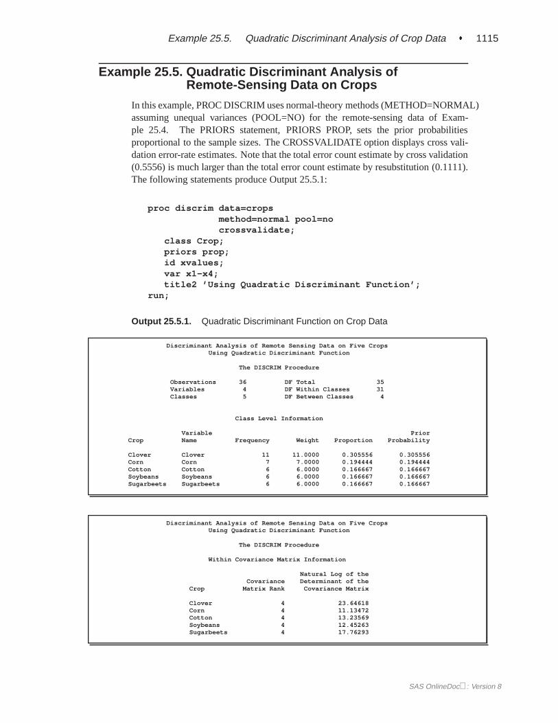
Example 25.5. Quadratic Discriminant Analysis of Crop Data � 1115
Example 25.5. Quadratic Discriminant Analysis ofRemote-Sensing Data on Crops
In this example, PROC DISCRIM uses normal-theory methods (METHOD=NORMAL)assuming unequal variances (POOL=NO) for the remote-sensing data of Exam-ple 25.4. The PRIORS statement, PRIORS PROP, sets the prior probabilitiesproportional to the sample sizes. The CROSSVALIDATE option displays cross vali-dation error-rate estimates. Note that the total error count estimate by cross validation(0.5556) is much larger than the total error count estimate by resubstitution (0.1111).The following statements produce Output 25.5.1:
proc discrim data=cropsmethod=normal pool=nocrossvalidate;
class Crop;priors prop;id xvalues;var x1-x4;title2 ’Using Quadratic Discriminant Function’;
run;
Output 25.5.1. Quadratic Discriminant Function on Crop Data
Discriminant Analysis of Remote Sensing Data on Five CropsUsing Quadratic Discriminant Function
The DISCRIM Procedure
Observations 36 DF Total 35Variables 4 DF Within Classes 31Classes 5 DF Between Classes 4
Class Level Information
Variable PriorCrop Name Frequency Weight Proportion Probability
Clover Clover 11 11.0000 0.305556 0.305556Corn Corn 7 7.0000 0.194444 0.194444Cotton Cotton 6 6.0000 0.166667 0.166667Soybeans Soybeans 6 6.0000 0.166667 0.166667Sugarbeets Sugarbeets 6 6.0000 0.166667 0.166667
Discriminant Analysis of Remote Sensing Data on Five CropsUsing Quadratic Discriminant Function
The DISCRIM Procedure
Within Covariance Matrix Information
Natural Log of theCovariance Determinant of the
Crop Matrix Rank Covariance Matrix
Clover 4 23.64618Corn 4 11.13472Cotton 4 13.23569Soybeans 4 12.45263Sugarbeets 4 17.76293
SAS OnlineDoc: Version 8
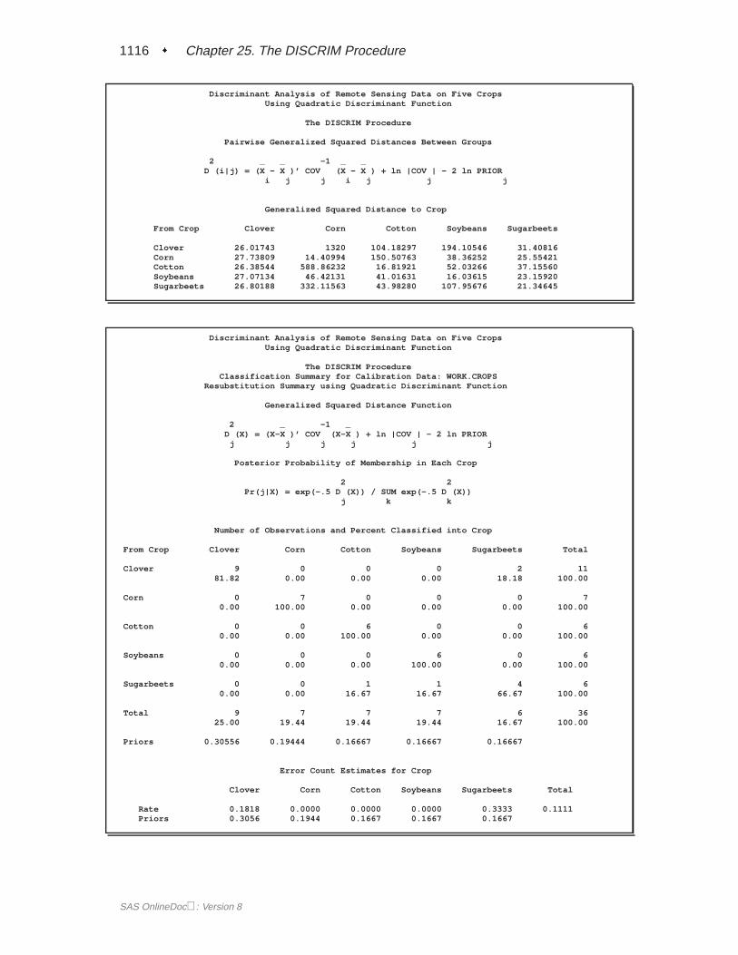
1116 � Chapter 25. The DISCRIM Procedure
Discriminant Analysis of Remote Sensing Data on Five CropsUsing Quadratic Discriminant Function
The DISCRIM Procedure
Pairwise Generalized Squared Distances Between Groups
2 _ _ -1 _ _D (i|j) = (X - X )’ COV (X - X ) + ln |COV | - 2 ln PRIOR
i j j i j j j
Generalized Squared Distance to Crop
From Crop Clover Corn Cotton Soybeans Sugarbeets
Clover 26.01743 1320 104.18297 194.10546 31.40816Corn 27.73809 14.40994 150.50763 38.36252 25.55421Cotton 26.38544 588.86232 16.81921 52.03266 37.15560Soybeans 27.07134 46.42131 41.01631 16.03615 23.15920Sugarbeets 26.80188 332.11563 43.98280 107.95676 21.34645
Discriminant Analysis of Remote Sensing Data on Five CropsUsing Quadratic Discriminant Function
The DISCRIM ProcedureClassification Summary for Calibration Data: WORK.CROPS
Resubstitution Summary using Quadratic Discriminant Function
Generalized Squared Distance Function
2 _ -1 _D (X) = (X-X )’ COV (X-X ) + ln |COV | - 2 ln PRIOR
j j j j j j
Posterior Probability of Membership in Each Crop
2 2Pr(j|X) = exp(-.5 D (X)) / SUM exp(-.5 D (X))
j k k
Number of Observations and Percent Classified into Crop
From Crop Clover Corn Cotton Soybeans Sugarbeets Total
Clover 9 0 0 0 2 1181.82 0.00 0.00 0.00 18.18 100.00
Corn 0 7 0 0 0 70.00 100.00 0.00 0.00 0.00 100.00
Cotton 0 0 6 0 0 60.00 0.00 100.00 0.00 0.00 100.00
Soybeans 0 0 0 6 0 60.00 0.00 0.00 100.00 0.00 100.00
Sugarbeets 0 0 1 1 4 60.00 0.00 16.67 16.67 66.67 100.00
Total 9 7 7 7 6 3625.00 19.44 19.44 19.44 16.67 100.00
Priors 0.30556 0.19444 0.16667 0.16667 0.16667
Error Count Estimates for Crop
Clover Corn Cotton Soybeans Sugarbeets Total
Rate 0.1818 0.0000 0.0000 0.0000 0.3333 0.1111Priors 0.3056 0.1944 0.1667 0.1667 0.1667
SAS OnlineDoc: Version 8
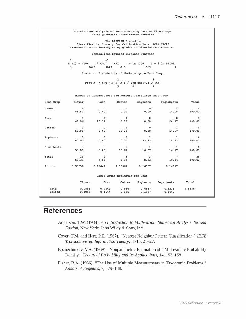
References � 1117
Discriminant Analysis of Remote Sensing Data on Five CropsUsing Quadratic Discriminant Function
The DISCRIM ProcedureClassification Summary for Calibration Data: WORK.CROPS
Cross-validation Summary using Quadratic Discriminant Function
Generalized Squared Distance Function
2 _ -1 _D (X) = (X-X )’ COV (X-X ) + ln |COV | - 2 ln PRIOR
j (X)j (X)j (X)j (X)j j
Posterior Probability of Membership in Each Crop
2 2Pr(j|X) = exp(-.5 D (X)) / SUM exp(-.5 D (X))
j k k
Number of Observations and Percent Classified into Crop
From Crop Clover Corn Cotton Soybeans Sugarbeets Total
Clover 9 0 0 0 2 1181.82 0.00 0.00 0.00 18.18 100.00
Corn 3 2 0 0 2 742.86 28.57 0.00 0.00 28.57 100.00
Cotton 3 0 2 0 1 650.00 0.00 33.33 0.00 16.67 100.00
Soybeans 3 0 0 2 1 650.00 0.00 0.00 33.33 16.67 100.00
Sugarbeets 3 0 1 1 1 650.00 0.00 16.67 16.67 16.67 100.00
Total 21 2 3 3 7 3658.33 5.56 8.33 8.33 19.44 100.00
Priors 0.30556 0.19444 0.16667 0.16667 0.16667
Error Count Estimates for Crop
Clover Corn Cotton Soybeans Sugarbeets Total
Rate 0.1818 0.7143 0.6667 0.6667 0.8333 0.5556Priors 0.3056 0.1944 0.1667 0.1667 0.1667
References
Anderson, T.W. (1984),An Introduction to Multivariate Statistical Analysis, SecondEdition, New York: John Wiley & Sons, Inc.
Cover, T.M. and Hart, P.E. (1967), “Nearest Neighbor Pattern Classification,”IEEETransactions on Information Theory, IT-13, 21–27.
Epanechnikov, V.A. (1969), “Nonparametric Estimation of a Multivariate ProbabilityDensity,”Theory of Probability and Its Applications, 14, 153–158.
Fisher, R.A. (1936), “The Use of Multiple Measurements in Taxonomic Problems,”Annals of Eugenics, 7, 179–188.
SAS OnlineDoc: Version 8
1118 � Chapter 25. The DISCRIM Procedure
Fix, E. and Hodges, J.L., Jr. (1959), “Discriminatory Analysis: Nonparametric Dis-crimination: Consistency Properties,”Report No. 4, Project No. 21-49-004,School of Aviation Medicine, Randolph Air Force Base, TX.
Friedman, J.H., Bentley, J.L., and Finkel, R.A. (1977), “An Algorithm for FindingBest Matches in Logarithmic Expected Time,”ACM Transactions on Mathemat-ical Software, 3, 209–226.
Fukunaga, K. and Kessel, D.L. (1973), “Nonparametric Bayes Error EstimationUsing Unclassified Samples,”IEEE Transactions on Information Theory, 19,434–440.
Glick, N. (1978), “Additive Estimators for Probabilities of Correct Classification,”Pattern Recognition, 10, 211–222.
Hand, D.J. (1981),Discrimination and Classification, New York: John Wiley & Sons,Inc.
Hand, D.J. (1982),Kernel Discriminant Analysis, New York: Research Studies Press.
Hand, D.J. (1986), “Recent Advances in Error Rate Estimation,”Pattern RecognitionLetters, 4, 335–346.
Hora, S.C. and Wilcox, J.B. (1982), “Estimation of Error Rates in Several-PopulationDiscriminant Analysis,”Journal of Marketing Research, XIX, 57–61.
Kendall, M.G., Stuart, A., and Ord, J.K. (1983),The Advanced Theory of Statistics,Vol. 3, Fourth Edition, New York: Macmillan Publishing Co., Inc.
Kshirsagar, A.M. (1972),Multivariate Analysis, New York: Marcel Dekker.
Lachenbruch, P.A. and Mickey, M.A. (1968), “Estimation of Error Rates in Discrim-inant Analysis,”Technometrics, 10, 1–10.
Lawley, D.N. (1959), “Tests of Significance in Canonical Analysis,”Biometrika, 46,59–66.
Morrison, D.F. (1976),Multivariate Statistical Methods, New York: McGraw-Hill.
Parzen, E. (1962), “On Estimation of a Probability Density Function and Mode,”Annals of Mathematical Statistics, 33, 1065–1076.
Perlman, M.D. (1980), “Unbiasedness of the Likelihood Ratio Tests for Equality ofSeveral Covariance Matrices and Equality of Several Multivariate Normal Popu-lations,”Annals of Statistics, 8, 247–263.
Rao, C. R. (1973),Linear Statistical Inference and Its Applications, Second Edition,New York: John Wiley & Sons, Inc.
Ripley, B.D. (1996),Pattern Recognition and Neural Networks, Cambridge: Cam-bridge University Press.
Rosenblatt, M. (1956), “Remarks on Some Nonparametric Estimates of a DensityFunction,”Annals of Mathematical Statistics, 27, 832–837.
Silverman, B. W. (1986),Density Estimation for Statistics and Data Analysis, NewYork: Chapman and Hall.
SAS OnlineDoc: Version 8
References � 1119
Snapinn, S.M. and Knoke, J.D. (1985), “An Evaluation of Smoothed ClassificationError-Rate Estimators,”Technometrics, 27, 199–206.
SAS OnlineDoc: Version 8
The correct bibliographic citation for this manual is as follows: SAS Institute Inc.,SAS/STAT ® User’s Guide, Version 8, Cary, NC: SAS Institute Inc., 1999.
SAS/STAT® User’s Guide, Version 8Copyright © 1999 by SAS Institute Inc., Cary, NC, USA.ISBN 1–58025–494–2All rights reserved. Produced in the United States of America. No part of this publicationmay be reproduced, stored in a retrieval system, or transmitted, in any form or by anymeans, electronic, mechanical, photocopying, or otherwise, without the prior writtenpermission of the publisher, SAS Institute Inc.U.S. Government Restricted Rights Notice. Use, duplication, or disclosure of thesoftware and related documentation by the U.S. government is subject to the Agreementwith SAS Institute and the restrictions set forth in FAR 52.227–19 Commercial ComputerSoftware-Restricted Rights (June 1987).SAS Institute Inc., SAS Campus Drive, Cary, North Carolina 27513.1st printing, October 1999SAS® and all other SAS Institute Inc. product or service names are registered trademarksor trademarks of SAS Institute Inc. in the USA and other countries.® indicates USAregistration.Other brand and product names are registered trademarks or trademarks of theirrespective companies.The Institute is a private company devoted to the support and further development of itssoftware and related services.