Embed Size (px)
Citation preview
The discrete entropic uncertainty relation
Hans Maassen
Goodbye, Jos! July 15, 2011.

History
Spring 1986. ‘Quantum Club’:
Jan Hilgevoord,
Dennis Diecks,
Michiel van Lambalgen
Dick Hoekzema,
Lou-Fe Feiner,
Jos & myself.
. . .?
Subject: ‘Entropic Uncertainty’
following Byalinicki-Birula, Heidelberg, October 1984
Remark Jos: Conjecture Karl Kraus:
For complementary observables A and B:
H(A) + H(B) ≥ log d .
During that meeting: Proof of conjecture by the same means:
Riesz-Thorin interpolation.

History
Spring 1986.
‘Quantum Club’:
Jan Hilgevoord,
Dennis Diecks,
Michiel van Lambalgen
Dick Hoekzema,
Lou-Fe Feiner,
Jos & myself.
. . .?
Subject: ‘Entropic Uncertainty’
following Byalinicki-Birula, Heidelberg, October 1984
Remark Jos: Conjecture Karl Kraus:
For complementary observables A and B:
H(A) + H(B) ≥ log d .
During that meeting: Proof of conjecture by the same means:
Riesz-Thorin interpolation.

History
Spring 1986. ‘Quantum Club’:
Jan Hilgevoord,
Dennis Diecks,
Michiel van Lambalgen
Dick Hoekzema,
Lou-Fe Feiner,
Jos & myself.
. . .?
Subject: ‘Entropic Uncertainty’
following Byalinicki-Birula, Heidelberg, October 1984
Remark Jos: Conjecture Karl Kraus:
For complementary observables A and B:
H(A) + H(B) ≥ log d .
During that meeting: Proof of conjecture by the same means:
Riesz-Thorin interpolation.

History
Spring 1986. ‘Quantum Club’:
Jan Hilgevoord,
Dennis Diecks,
Michiel van Lambalgen
Dick Hoekzema,
Lou-Fe Feiner,
Jos & myself.
. . .?
Subject:
‘Entropic Uncertainty’
following Byalinicki-Birula, Heidelberg, October 1984
Remark Jos: Conjecture Karl Kraus:
For complementary observables A and B:
H(A) + H(B) ≥ log d .
During that meeting: Proof of conjecture by the same means:
Riesz-Thorin interpolation.

History
Spring 1986. ‘Quantum Club’:
Jan Hilgevoord,
Dennis Diecks,
Michiel van Lambalgen
Dick Hoekzema,
Lou-Fe Feiner,
Jos & myself.
. . .?
Subject: ‘Entropic Uncertainty’
following Byalinicki-Birula, Heidelberg, October 1984
Remark Jos: Conjecture Karl Kraus:
For complementary observables A and B:
H(A) + H(B) ≥ log d .
During that meeting: Proof of conjecture by the same means:
Riesz-Thorin interpolation.

History
Spring 1986. ‘Quantum Club’:
Jan Hilgevoord,
Dennis Diecks,
Michiel van Lambalgen
Dick Hoekzema,
Lou-Fe Feiner,
Jos & myself.
. . .?
Subject: ‘Entropic Uncertainty’
following Byalinicki-Birula, Heidelberg, October 1984
Remark Jos:
Conjecture Karl Kraus:
For complementary observables A and B:
H(A) + H(B) ≥ log d .
During that meeting: Proof of conjecture by the same means:
Riesz-Thorin interpolation.

History
Spring 1986. ‘Quantum Club’:
Jan Hilgevoord,
Dennis Diecks,
Michiel van Lambalgen
Dick Hoekzema,
Lou-Fe Feiner,
Jos & myself.
. . .?
Subject: ‘Entropic Uncertainty’
following Byalinicki-Birula, Heidelberg, October 1984
Remark Jos: Conjecture Karl Kraus:
For complementary observables A and B:
H(A) + H(B) ≥ log d .
During that meeting: Proof of conjecture by the same means:
Riesz-Thorin interpolation.

History
Spring 1986. ‘Quantum Club’:
Jan Hilgevoord,
Dennis Diecks,
Michiel van Lambalgen
Dick Hoekzema,
Lou-Fe Feiner,
Jos & myself.
. . .?
Subject: ‘Entropic Uncertainty’
following Byalinicki-Birula, Heidelberg, October 1984
Remark Jos: Conjecture Karl Kraus:
For complementary observables A and B:
H(A) + H(B) ≥ log d .
During that meeting:
Proof of conjecture by the same means:
Riesz-Thorin interpolation.
History
Spring 1986. ‘Quantum Club’:
Jan Hilgevoord,
Dennis Diecks,
Michiel van Lambalgen
Dick Hoekzema,
Lou-Fe Feiner,
Jos & myself.
. . .?
Subject: ‘Entropic Uncertainty’
following Byalinicki-Birula, Heidelberg, October 1984
Remark Jos: Conjecture Karl Kraus:
For complementary observables A and B:
H(A) + H(B) ≥ log d .
During that meeting: Proof of conjecture by the same means:
Riesz-Thorin interpolation.

Success story
Jos wrote down the result in a Phys. Rev. Letter, and elaborated on it in his
Ph. D. thesis.
The Letter still is, for both of us, by far the most cited item on our publication
lists.
The inequality has been applied in quantum key distribution, entanglement
distillation, has been improved upon in special cases, and is generally
well-known in quantum information.
Aim of the talkBut it still eludes intuition. The question is rarely asked why it holds.
I would like to address this question today.

Success story
Jos wrote down the result in a Phys. Rev. Letter, and elaborated on it in his
Ph. D. thesis.
The Letter still is, for both of us, by far the most cited item on our publication
lists.
The inequality has been applied in quantum key distribution, entanglement
distillation, has been improved upon in special cases, and is generally
well-known in quantum information.
Aim of the talk
But it still eludes intuition. The question is rarely asked why it holds.
I would like to address this question today.

Success story
Jos wrote down the result in a Phys. Rev. Letter, and elaborated on it in his
Ph. D. thesis.
The Letter still is, for both of us, by far the most cited item on our publication
lists.
The inequality has been applied in quantum key distribution, entanglement
distillation, has been improved upon in special cases, and is generally
well-known in quantum information.
Aim of the talkBut it still eludes intuition. The question is rarely asked why it holds.
I would like to address this question today.

Success story
Jos wrote down the result in a Phys. Rev. Letter, and elaborated on it in his
Ph. D. thesis.
The Letter still is, for both of us, by far the most cited item on our publication
lists.
The inequality has been applied in quantum key distribution, entanglement
distillation, has been improved upon in special cases, and is generally
well-known in quantum information.
Aim of the talkBut it still eludes intuition. The question is rarely asked why it holds.
I would like to address this question today.

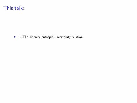
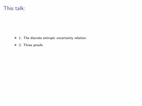
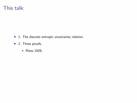
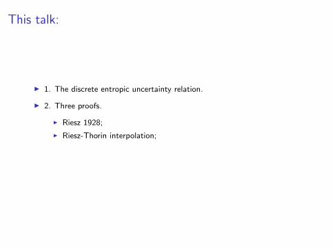
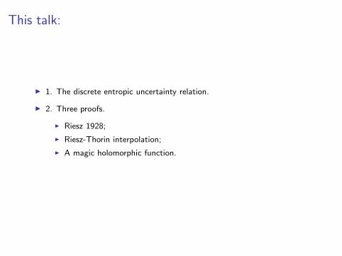
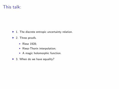
This talk:
I 1. The discrete entropic uncertainty relation.
I 2. Three proofs.
I Riesz 1928;
I Riesz-Thorin interpolation;
I A magic holomorphic function.
I 3. When do we have equality?
This talk:
I 1. The discrete entropic uncertainty relation.
I 2. Three proofs.
I Riesz 1928;
I Riesz-Thorin interpolation;
I A magic holomorphic function.
I 3. When do we have equality?
This talk:
I 1. The discrete entropic uncertainty relation.
I 2. Three proofs.
I Riesz 1928;
I Riesz-Thorin interpolation;
I A magic holomorphic function.
I 3. When do we have equality?
This talk:
I 1. The discrete entropic uncertainty relation.
I 2. Three proofs.
I Riesz 1928;
I Riesz-Thorin interpolation;
I A magic holomorphic function.
I 3. When do we have equality?
This talk:
I 1. The discrete entropic uncertainty relation.
I 2. Three proofs.
I Riesz 1928;
I Riesz-Thorin interpolation;
I A magic holomorphic function.
I 3. When do we have equality?
This talk:
I 1. The discrete entropic uncertainty relation.
I 2. Three proofs.
I Riesz 1928;
I Riesz-Thorin interpolation;
I A magic holomorphic function.
I 3. When do we have equality?
This talk:
I 1. The discrete entropic uncertainty relation.
I 2. Three proofs.
I Riesz 1928;
I Riesz-Thorin interpolation;
I A magic holomorphic function.
I 3. When do we have equality?

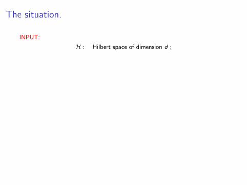
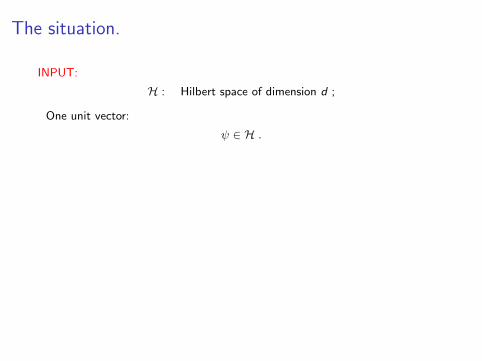
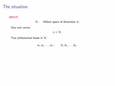
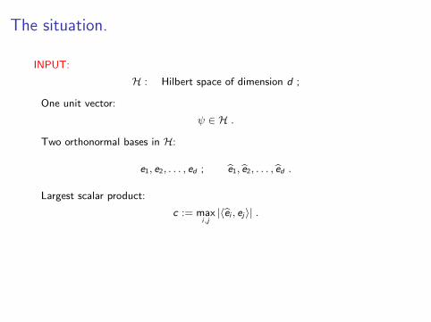
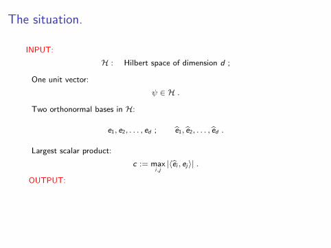
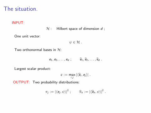
The situation.
INPUT:
H : Hilbert space of dimension d ;
One unit vector:
ψ ∈ H .
Two orthonormal bases in H:
e1, e2, . . . , ed ; be1,be2, . . . ,bed .
Largest scalar product:
c := maxi,j|〈bei , ej〉| .
OUTPUT: Two probability distributions:
πj := |〈ej , ψ〉|2 ; bπk := |〈bek , ψ〉|2 .

The situation.
INPUT:
H : Hilbert space of dimension d ;
One unit vector:
ψ ∈ H .
Two orthonormal bases in H:
e1, e2, . . . , ed ; be1,be2, . . . ,bed .
Largest scalar product:
c := maxi,j|〈bei , ej〉| .
OUTPUT: Two probability distributions:
πj := |〈ej , ψ〉|2 ; bπk := |〈bek , ψ〉|2 .
The situation.
INPUT:
H : Hilbert space of dimension d ;
One unit vector:
ψ ∈ H .
Two orthonormal bases in H:
e1, e2, . . . , ed ; be1,be2, . . . ,bed .
Largest scalar product:
c := maxi,j|〈bei , ej〉| .
OUTPUT: Two probability distributions:
πj := |〈ej , ψ〉|2 ; bπk := |〈bek , ψ〉|2 .
The situation.
INPUT:
H : Hilbert space of dimension d ;
One unit vector:
ψ ∈ H .
Two orthonormal bases in H:
e1, e2, . . . , ed ; be1,be2, . . . ,bed .
Largest scalar product:
c := maxi,j|〈bei , ej〉| .
OUTPUT: Two probability distributions:
πj := |〈ej , ψ〉|2 ; bπk := |〈bek , ψ〉|2 .
The situation.
INPUT:
H : Hilbert space of dimension d ;
One unit vector:
ψ ∈ H .
Two orthonormal bases in H:
e1, e2, . . . , ed ; be1,be2, . . . ,bed .
Largest scalar product:
c := maxi,j|〈bei , ej〉| .
OUTPUT: Two probability distributions:
πj := |〈ej , ψ〉|2 ; bπk := |〈bek , ψ〉|2 .
The situation.
INPUT:
H : Hilbert space of dimension d ;
One unit vector:
ψ ∈ H .
Two orthonormal bases in H:
e1, e2, . . . , ed ; be1,be2, . . . ,bed .
Largest scalar product:
c := maxi,j|〈bei , ej〉| .
OUTPUT: Two probability distributions:
πj := |〈ej , ψ〉|2 ; bπk := |〈bek , ψ〉|2 .
The situation.
INPUT:
H : Hilbert space of dimension d ;
One unit vector:
ψ ∈ H .
Two orthonormal bases in H:
e1, e2, . . . , ed ; be1,be2, . . . ,bed .
Largest scalar product:
c := maxi,j|〈bei , ej〉| .
OUTPUT:
Two probability distributions:
πj := |〈ej , ψ〉|2 ; bπk := |〈bek , ψ〉|2 .
The situation.
INPUT:
H : Hilbert space of dimension d ;
One unit vector:
ψ ∈ H .
Two orthonormal bases in H:
e1, e2, . . . , ed ; be1,be2, . . . ,bed .
Largest scalar product:
c := maxi,j|〈bei , ej〉| .
OUTPUT: Two probability distributions:
πj := |〈ej , ψ〉|2 ; bπk := |〈bek , ψ〉|2 .
The discrete entropic uncertainty relation
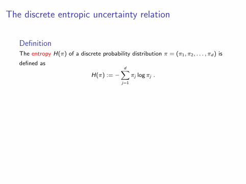
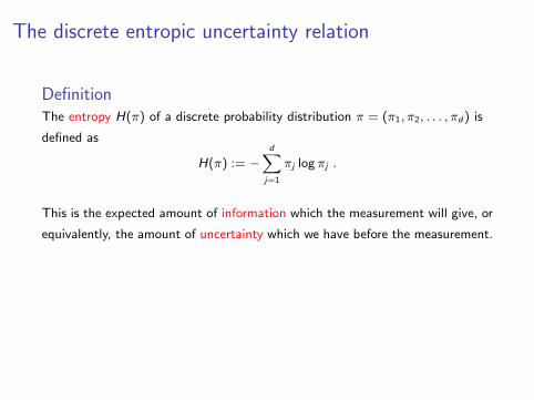
DefinitionThe entropy H(π) of a discrete probability distribution π = (π1, π2, . . . , πd) is
defined as
H(π) := −dX
j=1
πj log πj .
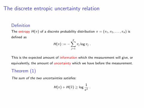
This is the expected amount of information which the measurement will give, or
equivalently, the amount of uncertainty which we have before the measurement.
Theorem (1)
The sum of the two uncertainties satisfies:
H(π) + H(bπ) ≥ log1
c2.
The discrete entropic uncertainty relation
DefinitionThe entropy H(π) of a discrete probability distribution π = (π1, π2, . . . , πd) is
defined as
H(π) := −dX
j=1
πj log πj .
This is the expected amount of information which the measurement will give, or
equivalently, the amount of uncertainty which we have before the measurement.
Theorem (1)
The sum of the two uncertainties satisfies:
H(π) + H(bπ) ≥ log1
c2.

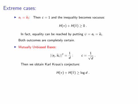
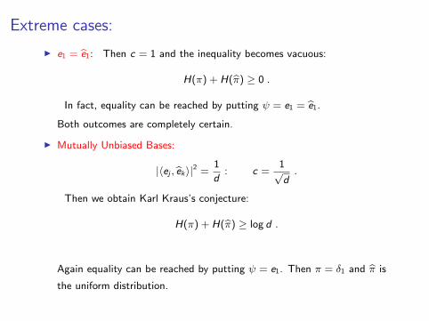
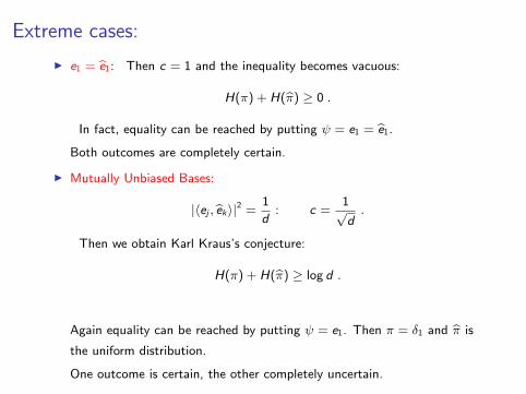
Extreme cases:
I e1 = be1: Then c = 1 and the inequality becomes vacuous:
H(π) + H(bπ) ≥ 0 .
In fact, equality can be reached by putting ψ = e1 = be1.
Both outcomes are completely certain.
I Mutually Unbiased Bases:
|〈ej ,bek〉|2 =1
d: c =
1√d.
Then we obtain Karl Kraus’s conjecture:
H(π) + H(bπ) ≥ log d .
Again equality can be reached by putting ψ = e1. Then π = δ1 and bπ is
the uniform distribution.
One outcome is certain, the other completely uncertain.

Extreme cases:
I e1 = be1:
Then c = 1 and the inequality becomes vacuous:
H(π) + H(bπ) ≥ 0 .
In fact, equality can be reached by putting ψ = e1 = be1.
Both outcomes are completely certain.
I Mutually Unbiased Bases:
|〈ej ,bek〉|2 =1
d: c =
1√d.
Then we obtain Karl Kraus’s conjecture:
H(π) + H(bπ) ≥ log d .
Again equality can be reached by putting ψ = e1. Then π = δ1 and bπ is
the uniform distribution.
One outcome is certain, the other completely uncertain.

Extreme cases:
I e1 = be1: Then c = 1 and the inequality becomes vacuous:
H(π) + H(bπ) ≥ 0 .
In fact, equality can be reached by putting ψ = e1 = be1.
Both outcomes are completely certain.
I Mutually Unbiased Bases:
|〈ej ,bek〉|2 =1
d: c =
1√d.
Then we obtain Karl Kraus’s conjecture:
H(π) + H(bπ) ≥ log d .
Again equality can be reached by putting ψ = e1. Then π = δ1 and bπ is
the uniform distribution.
One outcome is certain, the other completely uncertain.

Extreme cases:
I e1 = be1: Then c = 1 and the inequality becomes vacuous:
H(π) + H(bπ) ≥ 0 .
In fact, equality can be reached by putting ψ = e1 = be1.
Both outcomes are completely certain.
I Mutually Unbiased Bases:
|〈ej ,bek〉|2 =1
d: c =
1√d.
Then we obtain Karl Kraus’s conjecture:
H(π) + H(bπ) ≥ log d .
Again equality can be reached by putting ψ = e1. Then π = δ1 and bπ is
the uniform distribution.
One outcome is certain, the other completely uncertain.

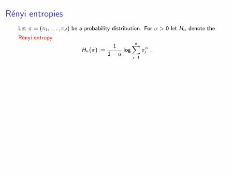
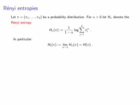
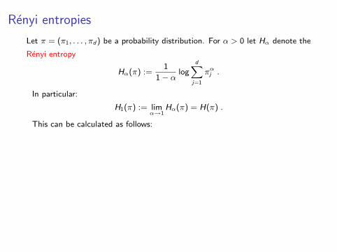
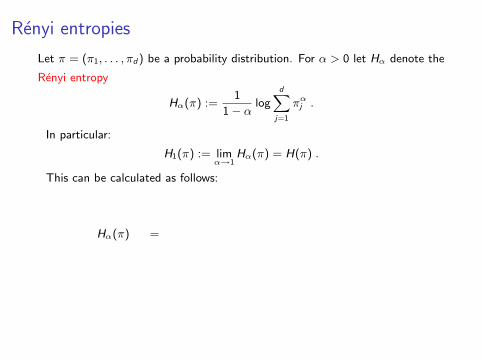
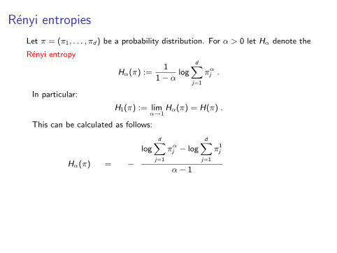
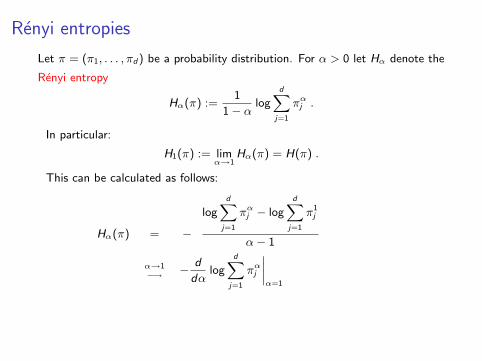
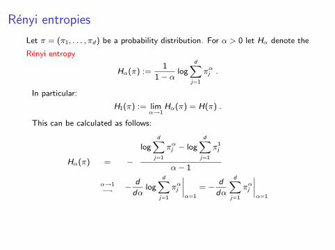
Renyi entropies
Let π = (π1, . . . , πd) be a probability distribution. For α > 0 let Hα denote the
Renyi entropy
Hα(π) :=1
1− α logdX
j=1
παj .
In particular:
H1(π) := limα→1
Hα(π) = H(π) .
This can be calculated as follows:
Hα(π) = −
logdX
j=1
παj − logdX
j=1
π1j
α− 1
α→1−→ − d
dαlog
dXj=1
παj
˛α=1
= − d
dα
dXj=1
παj
˛α=1
= −dX
j=1
πj log πj = H(π) .
Renyi entropies
Let π = (π1, . . . , πd) be a probability distribution. For α > 0 let Hα denote the
Renyi entropy
Hα(π) :=1
1− α logdX
j=1
παj .
In particular:
H1(π) := limα→1
Hα(π) = H(π) .
This can be calculated as follows:
Hα(π) =
−
logdX
j=1
παj − logdX
j=1
π1j
α− 1
α→1−→ − d
dαlog
dXj=1
παj
˛α=1
= − d
dα
dXj=1
παj
˛α=1
= −dX
j=1
πj log πj = H(π) .
Renyi entropies
Let π = (π1, . . . , πd) be a probability distribution. For α > 0 let Hα denote the
Renyi entropy
Hα(π) :=1
1− α logdX
j=1
παj .
In particular:
H1(π) := limα→1
Hα(π) = H(π) .
This can be calculated as follows:
Hα(π) = −
logdX
j=1
παj − logdX
j=1
π1j
α− 1
α→1−→ − d
dαlog
dXj=1
παj
˛α=1
= − d
dα
dXj=1
παj
˛α=1
= −dX
j=1
πj log πj = H(π) .
Renyi entropies
Let π = (π1, . . . , πd) be a probability distribution. For α > 0 let Hα denote the
Renyi entropy
Hα(π) :=1
1− α logdX
j=1
παj .
In particular:
H1(π) := limα→1
Hα(π) = H(π) .
This can be calculated as follows:
Hα(π) = −
logdX
j=1
παj − logdX
j=1
π1j
α− 1
α→1−→ − d
dαlog
dXj=1
παj
˛α=1
= − d
dα
dXj=1
παj
˛α=1
= −dX
j=1
πj log πj = H(π) .

Renyi entropies
Let π = (π1, . . . , πd) be a probability distribution. For α > 0 let Hα denote the
Renyi entropy
Hα(π) :=1
1− α logdX
j=1
παj .
In particular:
H1(π) := limα→1
Hα(π) = H(π) .
This can be calculated as follows:
Hα(π) = −
logdX
j=1
παj − logdX
j=1
π1j
α− 1
α→1−→ − d
dαlog
dXj=1
παj
˛α=1
= − d
dα
dXj=1
παj
˛α=1
= −dX
j=1
πj log πj
= H(π) .

Renyi entropies
Let π = (π1, . . . , πd) be a probability distribution. For α > 0 let Hα denote the
Renyi entropy
Hα(π) :=1
1− α logdX
j=1
παj .
In particular:
H1(π) := limα→1
Hα(π) = H(π) .
This can be calculated as follows:
Hα(π) = −
logdX
j=1
παj − logdX
j=1
π1j
α− 1
α→1−→ − d
dαlog
dXj=1
παj
˛α=1
= − d
dα
dXj=1
παj
˛α=1
= −dX
j=1
πj log πj = H(π) .
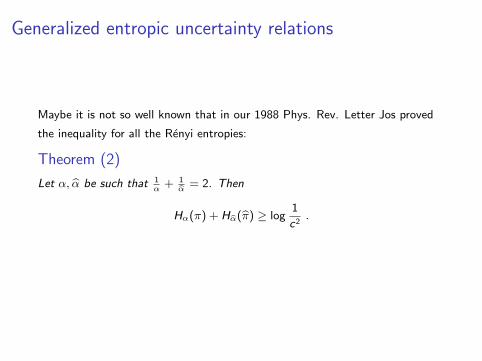
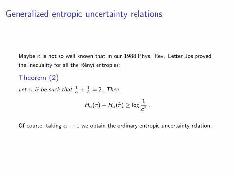
Generalized entropic uncertainty relations
Maybe it is not so well known that in our 1988 Phys. Rev. Letter Jos proved
the inequality for all the Renyi entropies:
Theorem (2)
Let α, bα be such that 1α
+ 1bα = 2. Then
Hα(π) + Hbα(bπ) ≥ log1
c2.
Of course, taking α→ 1 we obtain the ordinary entropic uncertainty relation.

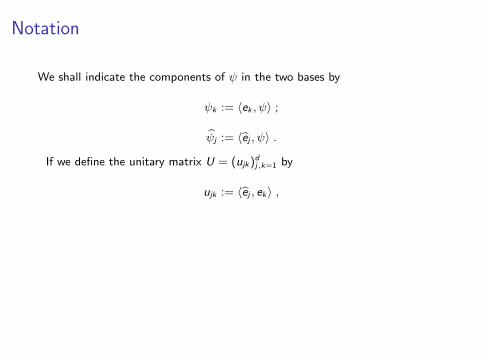
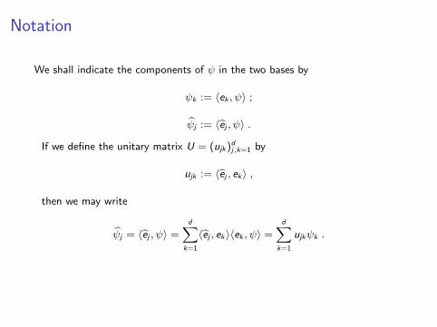
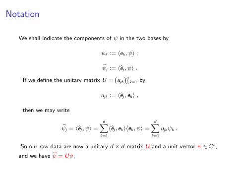
Notation
We shall indicate the components of ψ in the two bases by
ψk := 〈ek , ψ〉 ;
bψj := 〈bej , ψ〉 .
If we define the unitary matrix U = (ujk)dj,k=1 by
ujk := 〈bej , ek〉 ,
then we may write
bψj = 〈bej , ψ〉 =dX
k=1
〈bej , ek〉〈ek , ψ〉 =dX
k=1
ujkψk .
So our raw data are now a unitary d × d matrix U and a unit vector ψ ∈ Cn,
and we have bψ = Uψ.

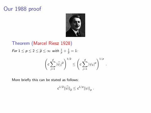
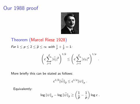
Our 1988 proof
Theorem (Marcel Riesz 1928)
For 1 ≤ p ≤ 2 ≤ bp ≤ ∞ with 1p
+ 1bp = 1: c
dXj=1
| bψj |bp!1/bp
≤
c
dXj=1
|ψk |p!1/p
.
More briefly this can be stated as follows:
c1/bp‖ bψ‖bp ≤ c1/p‖ψ‖p .
Equivalently:
log ‖ψ‖p − log ‖ bψ‖bp ≥„
1bp − 1
p
«log c .

Our 1988 proof
Theorem (Marcel Riesz 1928)
For 1 ≤ p ≤ 2 ≤ bp ≤ ∞ with 1p
+ 1bp = 1: c
dXj=1
| bψj |bp!1/bp
≤
c
dXj=1
|ψk |p!1/p
.
More briefly this can be stated as follows:
c1/bp‖ bψ‖bp ≤ c1/p‖ψ‖p .
Equivalently:
log ‖ψ‖p − log ‖ bψ‖bp ≥„
1bp − 1
p
«log c .

Our 1988 proof
Theorem (Marcel Riesz 1928)
For 1 ≤ p ≤ 2 ≤ bp ≤ ∞ with 1p
+ 1bp = 1: c
dXj=1
| bψj |bp!1/bp
≤
c
dXj=1
|ψk |p!1/p
.
More briefly this can be stated as follows:
c1/bp‖ bψ‖bp ≤ c1/p‖ψ‖p .
Equivalently:
log ‖ψ‖p − log ‖ bψ‖bp ≥„
1bp − 1
p
«log c .
Our 1988 proof
Theorem (Marcel Riesz 1928)
For 1 ≤ p ≤ 2 ≤ bp ≤ ∞ with 1p
+ 1bp = 1: c
dXj=1
| bψj |bp!1/bp
≤
c
dXj=1
|ψk |p!1/p
.
More briefly this can be stated as follows:
c1/bp‖ bψ‖bp ≤ c1/p‖ψ‖p .
Equivalently:
log ‖ψ‖p − log ‖ bψ‖bp ≥„
1bp − 1
p
«log c .
Our 1988 proof
Theorem (Marcel Riesz 1928)
For 1 ≤ p ≤ 2 ≤ bp ≤ ∞ with 1p
+ 1bp = 1: c
dXj=1
| bψj |bp!1/bp
≤
c
dXj=1
|ψk |p!1/p
.
More briefly this can be stated as follows:
c1/bp‖ bψ‖bp ≤ c1/p‖ψ‖p .
Equivalently:
log ‖ψ‖p − log ‖ bψ‖bp ≥„
1bp − 1
p
«log c .
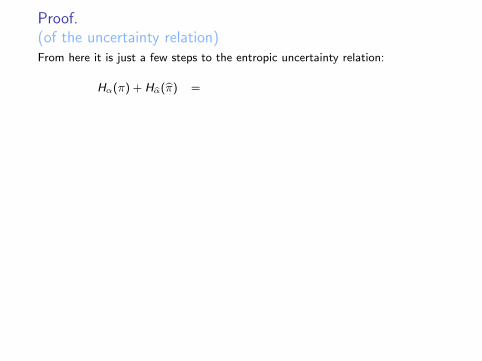
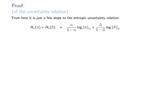
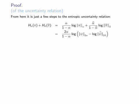
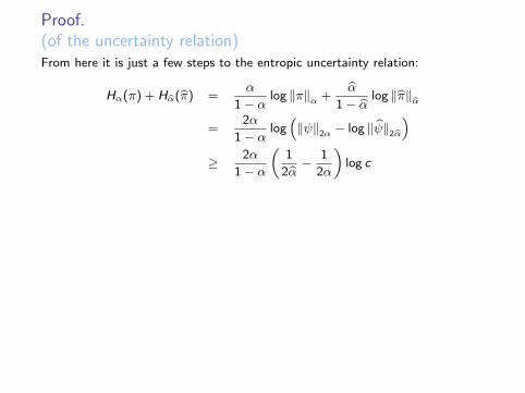
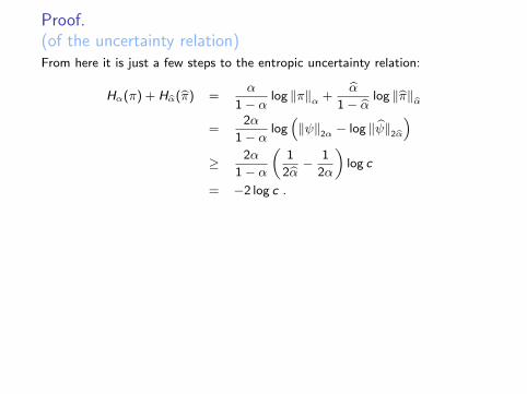
Proof.(of the uncertainty relation)
From here it is just a few steps to the entropic uncertainty relation:
Hα(π) + Hbα(bπ) =α
1− α log ‖π‖α +bα
1− bα log ‖bπ‖bα=
2α
1− α log“‖ψ‖2α − log ‖ bψ‖2bα
”≥ 2α
1− α
„1
2bα − 1
2α
«log c
= −2 log c .
Taking α→ 1 we also obtain the ordinary entropic uncertainty relation.
� � ��I proved the entropic uncertainty relation!
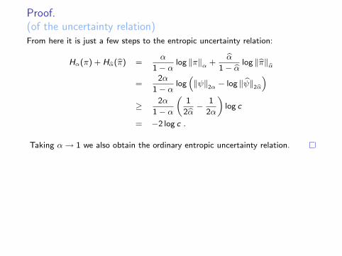
Proof.(of the uncertainty relation)From here it is just a few steps to the entropic uncertainty relation:
Hα(π) + Hbα(bπ) =α
1− α log ‖π‖α +bα
1− bα log ‖bπ‖bα=
2α
1− α log“‖ψ‖2α − log ‖ bψ‖2bα
”≥ 2α
1− α
„1
2bα − 1
2α
«log c
= −2 log c .
Taking α→ 1 we also obtain the ordinary entropic uncertainty relation.
� � ��I proved the entropic uncertainty relation!
Proof.(of the uncertainty relation)From here it is just a few steps to the entropic uncertainty relation:
Hα(π) + Hbα(bπ) =
α
1− α log ‖π‖α +bα
1− bα log ‖bπ‖bα=
2α
1− α log“‖ψ‖2α − log ‖ bψ‖2bα
”≥ 2α
1− α
„1
2bα − 1
2α
«log c
= −2 log c .
Taking α→ 1 we also obtain the ordinary entropic uncertainty relation.
� � ��I proved the entropic uncertainty relation!
Proof.(of the uncertainty relation)From here it is just a few steps to the entropic uncertainty relation:
Hα(π) + Hbα(bπ) =α
1− α log ‖π‖α +bα
1− bα log ‖bπ‖bα
=2α
1− α log“‖ψ‖2α − log ‖ bψ‖2bα
”≥ 2α
1− α
„1
2bα − 1
2α
«log c
= −2 log c .
Taking α→ 1 we also obtain the ordinary entropic uncertainty relation.
� � ��I proved the entropic uncertainty relation!
Proof.(of the uncertainty relation)From here it is just a few steps to the entropic uncertainty relation:
Hα(π) + Hbα(bπ) =α
1− α log ‖π‖α +bα
1− bα log ‖bπ‖bα=
2α
1− α log“‖ψ‖2α − log ‖ bψ‖2bα
”
≥ 2α
1− α
„1
2bα − 1
2α
«log c
= −2 log c .
Taking α→ 1 we also obtain the ordinary entropic uncertainty relation.
� � ��I proved the entropic uncertainty relation!
Proof.(of the uncertainty relation)From here it is just a few steps to the entropic uncertainty relation:
Hα(π) + Hbα(bπ) =α
1− α log ‖π‖α +bα
1− bα log ‖bπ‖bα=
2α
1− α log“‖ψ‖2α − log ‖ bψ‖2bα
”≥ 2α
1− α
„1
2bα − 1
2α
«log c
= −2 log c .
Taking α→ 1 we also obtain the ordinary entropic uncertainty relation.
� � ��I proved the entropic uncertainty relation!
Proof.(of the uncertainty relation)From here it is just a few steps to the entropic uncertainty relation:
Hα(π) + Hbα(bπ) =α
1− α log ‖π‖α +bα
1− bα log ‖bπ‖bα=
2α
1− α log“‖ψ‖2α − log ‖ bψ‖2bα
”≥ 2α
1− α
„1
2bα − 1
2α
«log c
= −2 log c .
Taking α→ 1 we also obtain the ordinary entropic uncertainty relation.
� � ��I proved the entropic uncertainty relation!

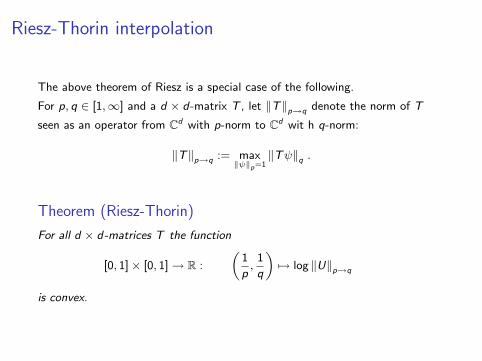
Riesz-Thorin interpolation
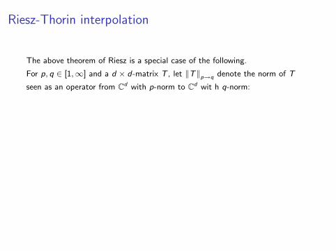
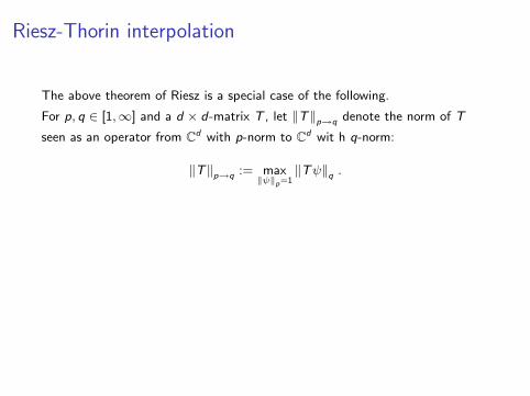
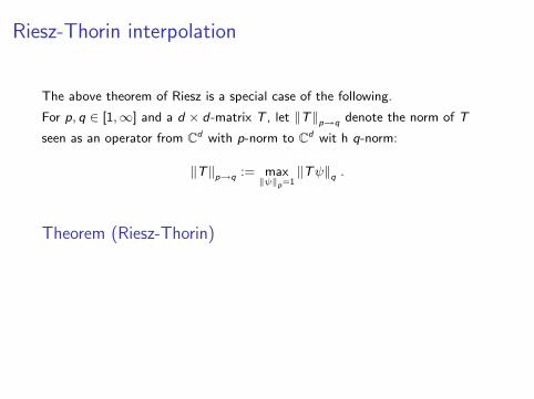
The above theorem of Riesz is a special case of the following.
For p, q ∈ [1,∞] and a d × d-matrix T , let ‖T‖p→q denote the norm of T
seen as an operator from Cd with p-norm to Cd wit h q-norm:
‖T‖p→q := max‖ψ‖p=1
‖Tψ‖q .
Theorem (Riesz-Thorin)
For all d × d-matrices T the function
[0, 1]× [0, 1]→ R :
„1
p,
1
q
«7→ log ‖U‖p→q
is convex.
Riesz-Thorin interpolation
The above theorem of Riesz is a special case of the following.
For p, q ∈ [1,∞] and a d × d-matrix T , let ‖T‖p→q denote the norm of T
seen as an operator from Cd with p-norm to Cd wit h q-norm:
‖T‖p→q := max‖ψ‖p=1
‖Tψ‖q .
Theorem (Riesz-Thorin)
For all d × d-matrices T the function
[0, 1]× [0, 1]→ R :
„1
p,
1
q
«7→ log ‖U‖p→q
is convex.
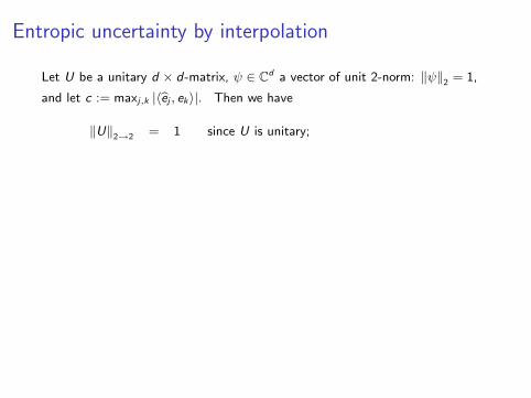
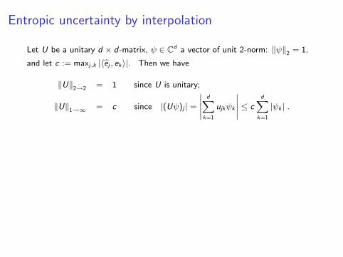
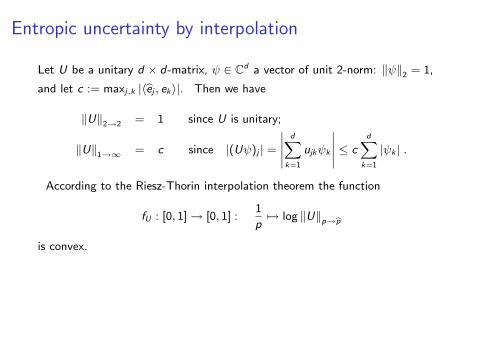
Entropic uncertainty by interpolation
Let U be a unitary d × d-matrix, ψ ∈ Cd a vector of unit 2-norm: ‖ψ‖2 = 1,
and let c := maxj,k |〈bej , ek〉|. Then we have
‖U‖2→2 = 1 since U is unitary;
‖U‖1→∞ = c since |(Uψ)j | =
˛˛
dXk=1
ujkψk
˛˛ ≤ c
dXk=1
|ψk | .
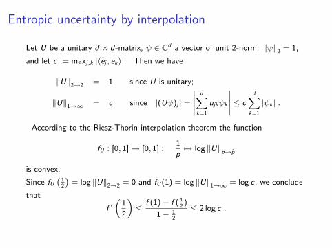
According to the Riesz-Thorin interpolation theorem the function
fU : [0, 1]→ [0, 1] :1
p7→ log ‖U‖p→bp
is convex.
Since fU`
12
´= log ‖U‖2→2 = 0 and fU(1) = log ‖U‖1→∞ = log c, we conclude
that
f ′„
1
2
«≤
f (1)− f ( 12)
1− 12
≤ 2 log c .
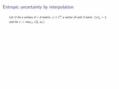
Entropic uncertainty by interpolation
Let U be a unitary d × d-matrix, ψ ∈ Cd a vector of unit 2-norm: ‖ψ‖2 = 1,
and let c := maxj,k |〈bej , ek〉|.
Then we have
‖U‖2→2 = 1 since U is unitary;
‖U‖1→∞ = c since |(Uψ)j | =
˛˛
dXk=1
ujkψk
˛˛ ≤ c
dXk=1
|ψk | .
According to the Riesz-Thorin interpolation theorem the function
fU : [0, 1]→ [0, 1] :1
p7→ log ‖U‖p→bp
is convex.
Since fU`
12
´= log ‖U‖2→2 = 0 and fU(1) = log ‖U‖1→∞ = log c, we conclude
that
f ′„
1
2
«≤
f (1)− f ( 12)
1− 12
≤ 2 log c .
Entropic uncertainty by interpolation
Let U be a unitary d × d-matrix, ψ ∈ Cd a vector of unit 2-norm: ‖ψ‖2 = 1,
and let c := maxj,k |〈bej , ek〉|. Then we have
‖U‖2→2 = 1 since U is unitary;
‖U‖1→∞ = c since |(Uψ)j | =
˛˛
dXk=1
ujkψk
˛˛ ≤ c
dXk=1
|ψk | .
According to the Riesz-Thorin interpolation theorem the function
fU : [0, 1]→ [0, 1] :1
p7→ log ‖U‖p→bp
is convex.
Since fU`
12
´= log ‖U‖2→2 = 0 and fU(1) = log ‖U‖1→∞ = log c, we conclude
that
f ′„
1
2
«≤
f (1)− f ( 12)
1− 12
≤ 2 log c .

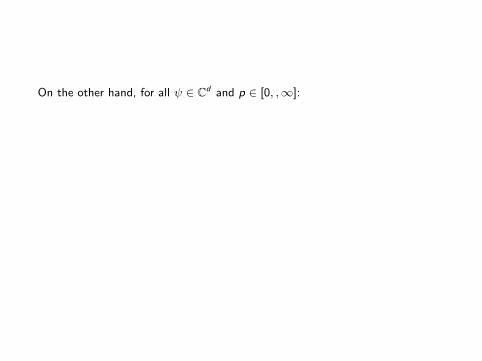
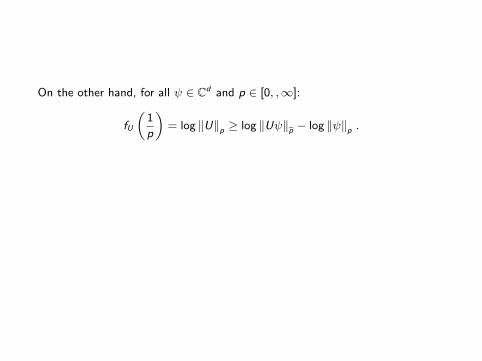
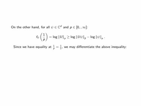
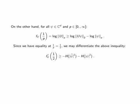
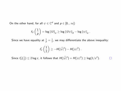
On the other hand, for all ψ ∈ Cd and p ∈ [0, ,∞]:
fU
„1
p
«= log ‖U‖p ≥ log ‖Uψ‖bp − log ‖ψ‖p .
Since we have equality at 1p
= 12, we may differentiate the above inequality:
f ′U
„1
2
«≥ −H(| bψ|2)− H(|ψ|2) .
Since f ′U( 12) ≤ 2 log c, it follows that H(| bψ|2) + H(|ψ|2) ≥ log(1/c2).
On the other hand, for all ψ ∈ Cd and p ∈ [0, ,∞]:
fU
„1
p
«= log ‖U‖p ≥ log ‖Uψ‖bp − log ‖ψ‖p .
Since we have equality at 1p
= 12, we may differentiate the above inequality:
f ′U
„1
2
«≥ −H(| bψ|2)− H(|ψ|2) .
Since f ′U( 12) ≤ 2 log c, it follows that H(| bψ|2) + H(|ψ|2) ≥ log(1/c2).
On the other hand, for all ψ ∈ Cd and p ∈ [0, ,∞]:
fU
„1
p
«= log ‖U‖p ≥ log ‖Uψ‖bp − log ‖ψ‖p .
Since we have equality at 1p
= 12, we may differentiate the above inequality:
f ′U
„1
2
«≥ −H(| bψ|2)− H(|ψ|2) .
Since f ′U( 12) ≤ 2 log c, it follows that H(| bψ|2) + H(|ψ|2) ≥ log(1/c2).
On the other hand, for all ψ ∈ Cd and p ∈ [0, ,∞]:
fU
„1
p
«= log ‖U‖p ≥ log ‖Uψ‖bp − log ‖ψ‖p .
Since we have equality at 1p
= 12, we may differentiate the above inequality:
f ′U
„1
2
«≥ −H(| bψ|2)− H(|ψ|2) .
Since f ′U( 12) ≤ 2 log c, it follows that H(| bψ|2) + H(|ψ|2) ≥ log(1/c2).
On the other hand, for all ψ ∈ Cd and p ∈ [0, ,∞]:
fU
„1
p
«= log ‖U‖p ≥ log ‖Uψ‖bp − log ‖ψ‖p .
Since we have equality at 1p
= 12, we may differentiate the above inequality:
f ′U
„1
2
«≥ −H(| bψ|2)− H(|ψ|2) .
Since f ′U( 12) ≤ 2 log c, it follows that H(| bψ|2) + H(|ψ|2) ≥ log(1/c2).
On the other hand, for all ψ ∈ Cd and p ∈ [0, ,∞]:
fU
„1
p
«= log ‖U‖p ≥ log ‖Uψ‖bp − log ‖ψ‖p .
Since we have equality at 1p
= 12, we may differentiate the above inequality:
f ′U
„1
2
«≥ −H(| bψ|2)− H(|ψ|2) .
Since f ′U( 12) ≤ 2 log c, it follows that H(| bψ|2) + H(|ψ|2) ≥ log(1/c2).

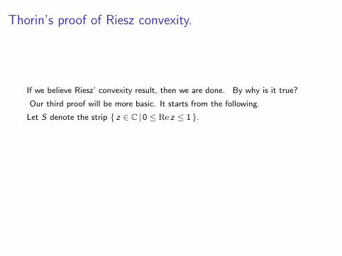
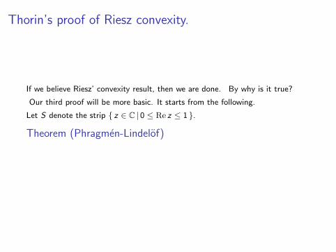
Thorin’s proof of Riesz convexity.
If we believe Riesz’ convexity result, then we are done. By why is it true?
Our third proof will be more basic. It starts from the following.
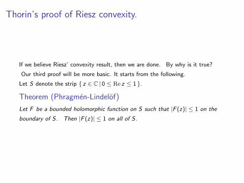
Let S denote the strip { z ∈ C | 0 ≤ Re z ≤ 1 }.
Theorem (Phragmen-Lindelof)
Let F be a bounded holomorphic function on S such that |F (z)| ≤ 1 on the
boundary of S. Then |F (z)| ≤ 1 on all of S.

Thorin’s proof of Riesz convexity.
If we believe Riesz’ convexity result, then we are done.
By why is it true?
Our third proof will be more basic. It starts from the following.
Let S denote the strip { z ∈ C | 0 ≤ Re z ≤ 1 }.
Theorem (Phragmen-Lindelof)
Let F be a bounded holomorphic function on S such that |F (z)| ≤ 1 on the
boundary of S. Then |F (z)| ≤ 1 on all of S.

Thorin’s proof of Riesz convexity.
If we believe Riesz’ convexity result, then we are done. By why is it true?
Our third proof will be more basic. It starts from the following.
Let S denote the strip { z ∈ C | 0 ≤ Re z ≤ 1 }.
Theorem (Phragmen-Lindelof)
Let F be a bounded holomorphic function on S such that |F (z)| ≤ 1 on the
boundary of S. Then |F (z)| ≤ 1 on all of S.

Thorin’s proof of Riesz convexity.
If we believe Riesz’ convexity result, then we are done. By why is it true?
Our third proof will be more basic. It starts from the following.
Let S denote the strip { z ∈ C | 0 ≤ Re z ≤ 1 }.
Theorem (Phragmen-Lindelof)
Let F be a bounded holomorphic function on S such that |F (z)| ≤ 1 on the
boundary of S.
Then |F (z)| ≤ 1 on all of S.
Thorin’s proof of Riesz convexity.
If we believe Riesz’ convexity result, then we are done. By why is it true?
Our third proof will be more basic. It starts from the following.
Let S denote the strip { z ∈ C | 0 ≤ Re z ≤ 1 }.
Theorem (Phragmen-Lindelof)
Let F be a bounded holomorphic function on S such that |F (z)| ≤ 1 on the
boundary of S. Then |F (z)| ≤ 1 on all of S.

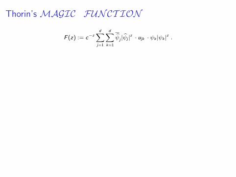
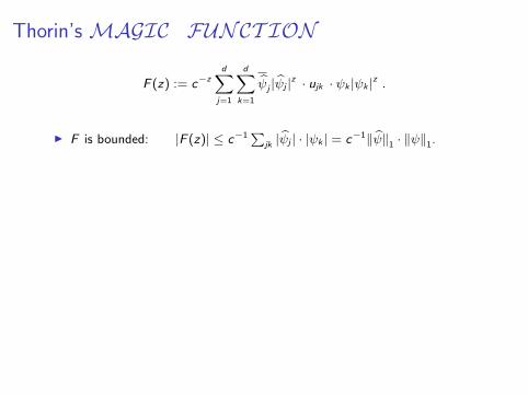
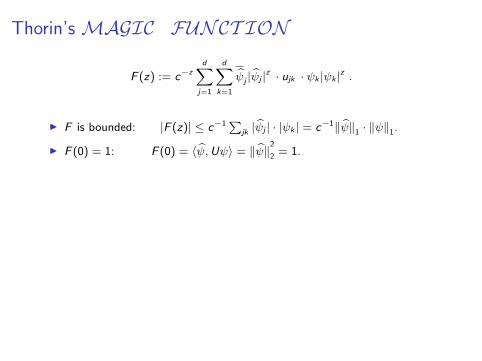
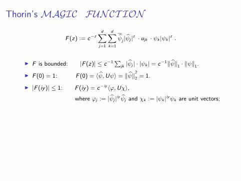
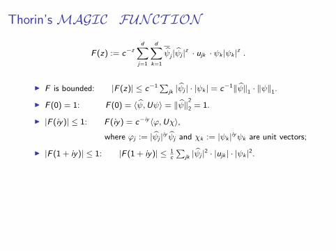
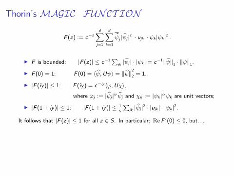
Thorin’s MAGIC FUNCT ION
F (z) := c−zdX
j=1
dXk=1
bψj | bψj |z · ujk · ψk |ψk |z .
I F is bounded: |F (z)| ≤ c−1Pjk | bψj | · |ψk | = c−1‖ bψ‖1 · ‖ψ‖1.
I F (0) = 1: F (0) = 〈 bψ,Uψ〉 = ‖ bψ‖22 = 1.
I |F (iy)| ≤ 1: F (iy) = c−iy 〈ϕ,Uχ〉,
where ϕj := | bψj |iy bψj and χk := |ψk |iyψk are unit vectors;
I |F (1 + iy)| ≤ 1: |F (1 + iy)| ≤ 1c
Pjk | bψj |2 · |ujk | · |ψk |2.
It follows that |F (z)| ≤ 1 for all z ∈ S . In particular: Re F ′(0) ≤ 0, but. . .
F ′(0) = − log c −dX
j=1
log | bψj | bψj(Uψ)j −dX
k=1
log |ψk |(U∗ bψ)kψk
= − log c − 1
2
`H(| bψ|2 + H(|ψ|2)
´.
The statement follows.
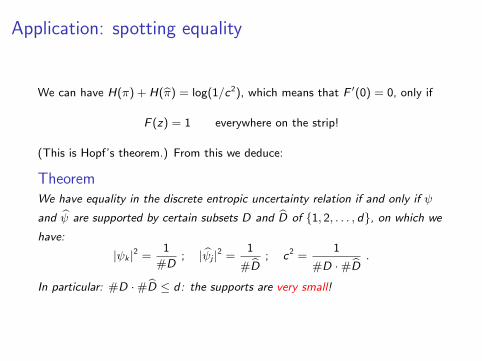
Application: spotting equality
We can have H(π) + H(bπ) = log(1/c2), which means that F ′(0) = 0, only if
F (z) = 1 everywhere on the strip!
(This is Hopf’s theorem.) From this we deduce:
TheoremWe have equality in the discrete entropic uncertainty relation if and only if ψ
and bψ are supported by certain subsets D and bD of {1, 2, . . . , d}, on which we
have:
|ψk |2 =1
#D; | bψj |2 =
1
#bD ; c2 =1
#D ·#bD .
In particular: #D ·#bD ≤ d: the supports are very small!
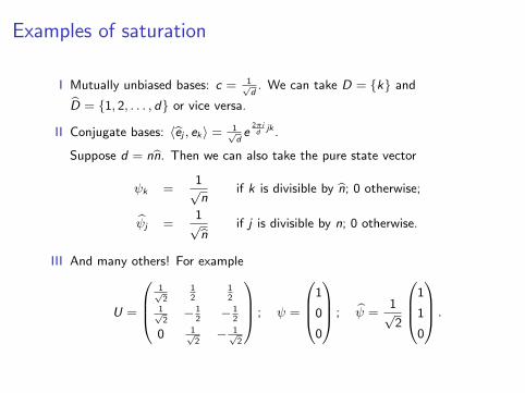
Examples of saturation
I Mutually unbiased bases: c = 1√d
. We can take D = {k} andbD = {1, 2, . . . , d} or vice versa.
II Conjugate bases: 〈bej , ek〉 = 1√d
e2πid
jk .
Suppose d = nbn. Then we can also take the pure state vector
ψk =1√n
if k is divisible by bn; 0 otherwise;
bψj =1√bn if j is divisible by n; 0 otherwise.
III And many others! For example
U =
0BB@1√2
12
12
1√2− 1
2− 1
2
0 1√2− 1√
2
1CCA ; ψ =
0BB@1
0
0
1CCA ; bψ =1√2
0BB@1
1
0
1CCA .
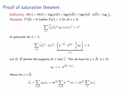
Proof of saturation theorem
Sufficiency: H(π) + H(bπ) = log(#D) + log(#bD) = log(#D ·#bD) = log 1c2 .
Necessity: F ′(0) = 0 implies F (z) = 1 for all z ∈ S :Xj,k
bψj | bψj |z ujk ψk |ψk |z = cz .
In particular for z = 1:Xj,k
| bψj |2 · |ψk |2 ·„
e−i bθj · e iθk · 1
cujk
«| {z }
=1!
= 1 .
Let D, bD denote the supports of ψ and bψ. The we have for j ∈ bD, k ∈ D:
ujk = c · e i(bθj−θk ) .
Hence for j ∈ bD:
bψj =Xk∈D
ujkψk = ce i bθjXk∈D
e−iθkψk = ce i bθjX
k
|ψk | .
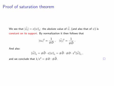
Proof of saturation theorem
We see that | bψj | = c‖ψ‖1: the abolute value of bψ, (and also that of ψ) is
constant on its support. By normalization it then follows that
|ψk |2 =1
#D, | bψj |2 =
1
#bD .
And also:
‖ bψ‖1 = #bD · c‖ψ‖1 = #bD ·#D · c2‖ bψ‖1 ,and we conclude that 1/c2 = #D ·#bD.