HAL Id: hal-00175643https://hal.archives-ouvertes.fr/hal-00175643v3

Submitted on 2 Nov 2009

HAL is a multi-disciplinary open accessarchive for the deposit and dissemination of sci-entific research documents, whether they are pub-lished or not. The documents may come fromteaching and research institutions in France orabroad, or from public or private research centers.

L’archive ouverte pluridisciplinaire HAL, estdestinée au dépôt et à la diffusion de documentsscientifiques de niveau recherche, publiés ou non,émanant des établissements d’enseignement et derecherche français ou étrangers, des laboratoirespublics ou privés.

The Dirichlet Markov EnsembleDjalil Chafai

To cite this version:Djalil Chafai. The Dirichlet Markov Ensemble. Journal of Multivariate Analysis, Elsevier, 2010, 101,pp.555-567. �10.1016/j.jmva.2009.10.013�. �hal-00175643v3�

The Dirichlet Markov Ensemble

Djalil Chafaı

Preprint – September 2007. Revised – August 2009, October 2009.

Abstract

We equip the polytope of n × n Markov matrices with the normalizedtrace of the Lebesgue measure of R

n2

. This probability space provides randomMarkov matrices, with i.i.d. rows following the Dirichlet distribution of mean(1/n, . . . , 1/n). We show that if M is such a random matrix, then the empiricaldistribution built from the singular values of

√nM tends as n → ∞ to a

Wigner quarter–circle distribution. Some computer simulations reveal strikingasymptotic spectral properties of such random matrices, still waiting for arigorous mathematical analysis. In particular, we believe that with probabilityone, the empirical distribution of the complex spectrum of

√nM tends as

n → ∞ to the uniform distribution on the unit disc of the complex plane, andthat moreover, the spectral gap of M is of order 1 − 1/

√n when n is large.

AMS 2000 Mathematical Subject Classification: 15A52; 15A51; 15A42; 60F15; 62H99.

Keywords: Random matrices; Markov matrices; Dirichlet laws; Spectral gap.

1 Introduction

Markov chains constitute an essential tool for the modelling of stochastic phenomenain Biology, Computer Science, Engineering, and Physics. It is nowadays well knownthat the trend to the equilibrium of ergodic Markov chains is related to the spectraldecomposition of their Markov transition matrix, see for instance [Sen06, SC97,CSC08]. The corresponding literature is very rich, and many statisticians includingfor instance the famous Persi Diaconis contributed to this subject, by providingquantitative bounds for various concrete specific Markov chains. But how a Markovchain behaves when its Markov transition matrix is taken arbitrarily in the setof Markov matrices? The present paper aims to provide some partial answers tothis natural concrete question. From the statistical point of view, one can thinkabout considering random Markov matrices following the “uniform law” over theset of Markov matrices, which corresponds to a maximum entropy distribution orBayesian prior, see for example [DR06]. Recall that a n × n square real matrix Mis Markov if and only if its entries are non–negative and each row sums up to 1, i.e.if and only if each row of M belongs to the simplex

Λn = {(x1, . . . , xn) ∈ [0, 1]n such that x1 + · · · + xn = 1} (1)

1

which is the portion of the unit ‖·‖1-sphere of Rn with non–negative coordinates.The spectrum of a Markov matrix lies in the unit disc {z ∈ C; |z| 6 1}, contains 1,and is symmetric with respect to the real axis in the complex plane.

Uniform distribution on Markov matrices

Let Mn be the set of n× n Markov matrices. We need to give a precise meaning tothe notion of uniform distribution on Mn. This set is a convex compact polytopewith n(n − 1) degrees of freedom if n > 1. It has zero Lebesgue measure in Rn2

.Since Mn is a polytope of Rn2

(i.e. intersection of half spaces), the trace of theLebesgue measure on it makes sense and coincides with a cone measure1, despite itszero Lebesgue measure in Rn2

. Since Mn is additionally compact, the trace of theLebesgue measure can be normalized into a probability distribution. We thus definethe uniform distribution U(Mn) on Mn as the normalized trace of the Lebesguemeasure of R

n2

. The following theorem relates U(Mn) to the Dirichlet distribution.

Theorem 1.1 (Dirichlet Markov Ensemble). We have M ∼ U(Mn) if and only

if the rows of M are i.i.d. and follow the Dirichlet law of mean ( 1n, . . . , 1

n). The

probability distribution U(Mn) is invariant by permutations of rows and columns.

Corollary 1.2. If M ∼ U(Mn) then for every 1 6 i, j 6 n, Mi,j ∼ Beta(1, n − 1)and for every 1 6 i, i′, j, j′ 6 n,

Cov(Mi,j,Mi′,j′) =

0 if i 6= i′

n−1n2(n+1)

if i = i′ and j = j′

− 1n2(n+1)

if i = i′ and j 6= j′.

Moreover Mi,j and Mi′,j′ are independent if and only if i 6= i′.

The set Mn is also a compact semi–group for the matrix product. The followingtwo theorems concern the translation invariance of U(Mn) and the question of theexistence of an idempotent probability distribution on Mn.

Theorem 1.3 (Translation invariance). For every T ∈ Mn, the law U(Mn) is

invariant by the left translation M 7→ TM if and only if T is a permutation matrix.

The same holds true for the right translation M 7→ MT.

Theorem 1.4 (Idempotent distributions). There is no probability distribution on

Mn, absolutely continuous with respect to U(Mn), with full support, and which is

invariant by every left translations M 7→ TM where T runs over Mn. The same

holds true for right translations.

The proofs of theorems 1.1, 1.3, 1.4 and corollary 1.2 are given in section 2.

1Actually, one can define the trace of the Lebesgue measure and then the uniform distributionon many compact subsets of the Euclidean space, by using the notion of Hausdorff measure [Fal03].See also [CPSV09] for an approximate simulation method based on billiards and random reflections.

2

Asymptotic behavior of singular values and eigenvalues

The spectral properties of large dimensional random matrices are connected to manyareas of mathematics, see for instance the books [Meh04, HP00, BS06, AGZ09,For09, ER05] and the survey [Bai99]. If M ∼ U(Mn), then almost surely, the realmatrix M is invertible, non–normal, with neither independent nor centered entries.The singular values of certain large dimensional centered random matrices withindependent rows is considered for instance in [Aub06] and [MP06, PP07].

For any square n × n matrix A with real or complex entries, let the complexeigenvalues λ1(A), . . . , λn(A) of A be labeled so that |λ1(A)| > · · · > |λn(A)|. Thespectral radius of A is thus given by |λ1(A)| = max16k6n |λk(A)|. The empirical

spectral distribution (ESD) of A is the discrete probability distribution on C withat most n atoms defined by

1

n

n∑

k=1

δλk(A).

The singular values s1(A) > · · · > sn(A) > 0 of A are the eigenvalues of the positivesemi–definite Hermitian matrix (AA∗)1/2 where

A∗ = A⊤

denotes the conjugate transpose of A. Namely, for every 1 6 k 6 n,

sk(A) = λk(√

AA∗) =√

λk(AA∗).

Note that AA∗ and A∗A share the same spectrum. The atoms of the ESD of√AA∗ are s1(A), . . . , sn(A). The singular values of A have a clear geometrical

interpretation: the linear operator A maps the unit ball to an ellipsoid, and thesingular values of A are exactly the half–lengths of its principal axes. In particular,s1(A) = max‖x‖

2=1 ‖Ax‖2 = ‖A‖2→2 while sn(A) = min‖x‖

2=1 ‖Ax‖2 = ‖A−1‖−1

2→2.Moreover, A has exactly rank(A) non zero singular values. The relationship betweenthe eigenvalues and the singular values are captured by the Weyl–Horn inequalities

∀k ∈ {1, . . . , n},k∏

i=1

|λi(A)| 6

k∏

i=1

si(A) with equality when k = n,

see [Hor54, Wey49]. If A is normal, i.e. AA∗ = A∗A, then sk(A) = |λk(A)| forevery 1 6 k 6 n. Back to our Dirichlet Markov Ensemble, if M ∼ U(Mn) then M isalmost surely a non–normal matrix, and thus one cannot express the singular valuesof M in terms of the eigenvalues of M. The following theorem gives the asymptoticbehavior of the empirical distribution built from the singular values of M.

Theorem 1.5 (Singular values for Dirichlet Markov Ensemble). Let (Xi,j)16i,j<∞be an infinite array of i.i.d. exponential random variables of unit mean. For every

n, let M be the n × n random matrix defined for every 1 6 i, j 6 n by

Mi,j =Xi,j

∑nk=1 Xi,k

.

3

Probability distribution name Support Lebesgue density

Circle or circular law Cσ {z ∈ C; |z| 6 σ} ⊂ C z 7→ (πσ2)−1

Wigner semi–circle distribution Wσ [−2σ, +2σ] ⊂ R x 7→ (2πσ2)−1√

4σ2 − x2

Wigner quarter–circle distribution Qσ [0, 2σ] ⊂ R x 7→ (πσ2)−1√

4σ2 − x2

Marchenko–Pastur distribution Pσ [0, 4σ2] ⊂ R x 7→ (2πσ2x)−1√

x(4σ2 − x)

Table 1: Some of the remarkable probability distributions in random matrices.

Then M ∼ U(Mn) and

P

(

1

n

n∑

k=1

δλk(nMM⊤)w−→

n→∞P1

)

= 1

wherew→ denotes the weak convergence of probability distributions and P1 the Marchenko–

Pastur distribution defined in table 1. In other words,

P

(

1

n

n∑

k=1

δsk(√

nM)w−→

n→∞Q1

)

= 1

where Q1 denotes the Wigner quarter–circle distribution defined in table 1.

Following the notations of table 1, for every real fixed parameter σ > 0, everyreal random variable W , and every complex random variable Z = U +

√−1V with

U = RealPart(Z) and V = ImaginaryPart(Z), we have, by a change of variables,(

W 2 ∼ Pσ ⇔ |W | ∼ Qσ

)

and(

W ∼ Wσ ⇒ W 2 ∼ Pσ and |W | ∼ Qσ

)

.

Moreover, we have, simply by using the Cramer-Wold theorem,

Z ∼ C2σ ⇔(

RealPart(e√−1θZ) ∼ Wσ for every θ ∈ [0, 2π)

)

.

In particular, we have

Z ∼ C2σ ⇒ U ∼ Wσ and V ∼ Wσ.

Beware however that U and V are not independent random variables! Furthermore,if P(|Z| = σ; V > 0) = 1 then Z follows the uniform distribution over the upperhalf circle of radius σ if and only if U follows the so–called arc–sine distribution on[−σ, +σ] ⊂ R with Lebesgue density x 7→ (π

√σ2 − x2)−1.

The proof of theorem 1.5 is given in section 3. Since |λ1(A)| 6 s1(A) for anysquare matrix A, and since λ1(M) = 1, we have for every n > 1

s1(M) > |λ1(M)| = 1.

However, theorem 1.5 implies in particular that almost surely

1

nCard

{

1 6 k 6 n such that sk(M) >2√n

}

−→n→∞

0.

4

Random Q-matrices

Bryc, Dembo, and Jiang studied in [BDJ06] the limiting spectral distribution of ran-

dom Hankel, Markov, and Toeplitz matrices. Let us explain briefly what they meanby “random Markov matrices”. They proved the following theorem (see [BDJ06, th.1.3] and also [BS08]) : let (Xi,j)1<i<j<∞ be an infinite triangular array of i.i.d. realrandom variables of mean 0 and variance 1. Let Q be the symmetric n× n randommatrix defined for every 1 6 i 6 j 6 n by Qi,j = Qj,i = Xi,j if i < j, and

Qi,i = −∑

16k6nk 6=i

Qi,k for every 1 6 i 6 n.

Then, almost surely, the ESD of n−1/2 Q converges as n → ∞ to the free convolution2

of a semi–circle law and a standard Gaussian law.This result gives an answer to a precise question raised by Bai in his 1999 review

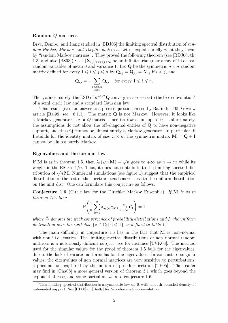
article [Bai99, sec. 6.1.1]. The matrix Q is not Markov. However, it looks likea Markov generator, i.e. a Q-matrix, since its rows sum up to 0. Unfortunately,the assumptions do not allow the off–diagonal entries of Q to have non–negativesupport, and thus Q cannot be almost surely a Markov generator. In particular, ifI stands for the identity matrix of size n × n, the symmetric matrix M = Q + Icannot be almost surely Markov.

Eigenvalues and the circular law

If M is as in theorem 1.5, then λ1(√

nM) =√

n goes to +∞ as n → ∞ while itsweight in the ESD is 1/n. Thus, it does not contribute to the limiting spectral dis-tribution of

√nM. Numerical simulations (see figure 1) suggest that the empirical

distribution of the rest of the spectrum tends as n → ∞ to the uniform distributionon the unit disc. One can formulate this conjecture as follows.

Conjecture 1.6 (Circle law for the Dirichlet Markov Ensemble). If M is as in

theorem 1.5, then

P

(

1

n

n∑

k=1

δλk(√

nM)w−→

n→∞C1

)

= 1

wherew→ denotes the weak convergence of probability distributions and C1 the uniform

distribution over the unit disc {z ∈ C; |z| 6 1} as defined in table 1.

The main difficulty in conjecture 1.6 lies in the fact that M is non–normalwith non i.i.d. entries. The limiting spectral distributions of non–normal randommatrices is a notoriously difficult subject, see for instance [TVK08]. The methodused for the singular values for the proof of theorem 1.5 fails for the eigenvalues,due to the lack of variational formulas for the eigenvalues. In contrast to singularvalues, the eigenvalues of non–normal matrices are very sensitive to perturbations,a phenomenon captured by the notion of pseudo–spectrum [TE05]. The readermay find in [Cha08] a more general version of theorem 3.1 which goes beyond theexponential case, and some partial answers to conjecture 1.6.

2This limiting spectral distribution is a symmetric law on R with smooth bounded density ofunbounded support. See [HP00] or [Bia97] for Voiculescu’s free convolution.

5

Sub–dominant eigenvalue

The fact that non–centered entries produce an explosive extremal eigenvalue wasalready noticed in various situations, see for instance [And90], [Sil94], [BDJ06, th.1.4], [BS07], and [Cha07]. It is natural to ask about the asymptotic behavior (conver-gence and fluctuations) of the sub–dominant eigenvalue λ2(M) when M ∼ U(Mn).The reader may find some answers in [GN03, GONS00], and may forge new conjec-tures from our simulations (see figures 2 and 3). For instance, by analogy with theComplex Ginibre Ensemble [Kos92, Rid03], one can state the following:

Conjecture 1.7 (Behavior of sub–dominant eigenvalue and spectral gap). If M is

as in theorem 1.5, then λ1(M) = 1 while

P

(

limn→∞

√n |λ2(M)| = 1

)

= 1.

In particular, the spectral gap 1 − |λ2(M)| of M is of order 1 − 1/√

n for large

n. Moreover, there exist deterministic sequences (an) and (bn) and a probability

distribution G on R such that

bn(|λ2(M)| − an)d−→

n→∞G

whered→ denotes the convergence in law.

There is not clear indication that G is a Gumbel distribution as for the Com-plex Ginibre Ensemble. Moreover, our simulations suggest that the sub–dominanteigenvalue is real with positive probability (depends on n), which is not surprisingknowing [Ede97, EKS94]. Note that Goldberg and Neumann have shown [GN03]that if X is an n×n random matrix with i.i.d. rows such that for every 1 6 i, j, j′ 6 n,

E[Xi,j] =1

n, and Var(Xi,j) = O

(

1

n2

)

, and |Cov(Xi,j,Xi,j′)| = O

(

1

n3

)

then P(|λ2(X)| 6 r) > p for any p ∈ (0, 1), any 0 < r < 1, and large enough n. Thisis the case if we set X = M.

Other distributions

The Dirichlet distribution of dimension n and mean ( 1n, . . . , 1

n) is the uniform distri-

bution on the simplex Λn defined by (1). One can replace the uniform distributionby a Dirichlet distribution of dimension n and arbitrary mean. The argument usedin the proof of theorem 1.5 remains the same due to the very similar construction ofDirichlet distributions by projection from i.i.d. Gamma random variables. One canalso replace the ‖·‖1-norm by any other ‖·‖p-norm, and investigate the limiting spec-tral distribution of the corresponding random matrices. This case can be handledwith the construction of the uniform distribution by projection proposed in [SZ90].Replacing the non–negative portion of spheres by the non–negative portion of ballsis also possible by using [BGMN05]. More generally, one can consider random ma-trices with independent rows. The case of the uniform distribution on the whole

6

unit ‖·‖p–ball of Rn is considered for instance by in [Aub06] by using [BGMN05]together with random matrices results for i.i.d. centered entries. It is crucial hereto have an explicit construction of the distribution from an i.i.d. array. For the linkwith the sampling of convex bodies, see [Aub07]. The case of matrices with i.i.d.rows following a log-concave isotropic distribution is considered in the recent work[PP07], by using recently developed results on log-concave measures. The readermay find a universal version of theorem 3.1 in [Cha08], where the exponential lawis replaced by an arbitrary law.

Doubly Stochastic matrices

The Birkhoff or transportation polytope is the set of n×n doubly stochastic matrices,i.e. matrices which are Markov and have a Markov transpose. Each n × n doublystochastic matrix corresponds to a transportation map of n unit masses into n boxesof unit mass (matching), and conversely, each transportation map of this kind is an × n doubly stochastic matrix. Geometrically, the Birkhoff polytope is a convexcompact subset of Mn of zero Lebesgue measure in R

n2

and (n − 1)2 degrees offreedom if n > 1. As for Mn, one can define the uniform distribution as thenormalized trace of the Lebesgue measure. However, we ignore if this distributionhas a probabilistic representation that allows exact simulation as for U(Mn). Thespectral behavior of random doubly stochastic matrices was considered in the Physicsliterature, see for instance [Ber01]. On the purely discrete side, the Birkhoff polytopeis also related to magic squares, transportation polytopes and contingency tables,see [DE87, DE85] and [DG95]. Note also that if M is Markov, then MM⊤ and12(M+M⊤) are not Markov in general. However, this is the case when M is doubly

stochastic. The Birkhoff-von Neumann theorem states that the extremal points ofthe Birkhoff polytope are exactly the permutation matrices. The reader may findnice spectral results on random uniform permutation matrices in [HKOS00, Wie00]and references therein.

Another interesting polytope of matrices is the set of symmetric n × n Markovmatrices, which is a convex compact polytope of zero Lebesgue measure in Rn2

with12n(n − 1) degrees of freedom if n > 1. As for Mn, one can define the uniform

distribution as the normalized trace of the Lebesgue measure. However, we ignoreif this distribution has a probabilistic representation that allows simulation as forU(Mn). One can ask about the spectral properties of the corresponding randomsymmetric Markov matrices. Note that these matrices are doubly stochastic, but theconverse is false except when n = 1 or n = 2. Our construction of U(Mn) in theorem1.5 corresponds in the Markovian probabilistic jargon to a random conductancemodel on the complete oriented graph. The study of the spectral properties ofrandom reversible Markov conductance models on the complete non–oriented graphcan be found in [Cha09, BCC08, BCC09]. For other graphs, the reader may findsome clues in [BDPX05].

Let M be as in theorem 1.5. Numerical simulations suggest that almost surely,the ESD of the symmetric matrix 1

2(M + M⊤) tends, as n → ∞, to a semi–circle

Wigner distribution.If U is an n × n unitary matrix, then (|Ui,j|2)16i,j6n is a doubly stochastic

matrix. These doubly stochastic matrices are called uni–stochastic or unitary-

7

stochastic. There exists doubly stochastic matrices which are not uni–stochastic,see [BEK+05] and [Tan01]. However, every permutation matrix is orthogonal andthus uni–stochastic. The Haar measure on the unitary group induces a probabil-ity distribution on the set of uni–stochastic matrices. How about the asymptoticspectral properties of the corresponding random matrices?

Perron–Frobenius eigenvector (invariant vector)

If M ∼ U(Mn), then almost surely, all the entries of M are non-zero, and inparticular, M is almost surely recurrent irreducible and aperiodic. By a theoremof Perron and Frobenius [Sen06], it follows that almost surely, the eigenspace ofM⊤ associated to the eigenvalue 1 is of dimension 1 and contains a unique vectorwith non–negative entries and unit ‖·‖1-norm. One can ask about the asymptoticbehavior of this vector as n → ∞. For a fixed n, the distribution of this vector isthe distribution of the rows of the infinite product of random matrices limk→∞ Mk.

2 Structure of the Dirichlet Markov Ensemble

Let Λn be as in (1). For any a ∈ (0,∞)n, the Dirichlet distribution Dn(a1, . . . , an),supported by Λn, is defined as the distribution of

1

‖G‖1

G =

(

G1

G1 + · · ·+ Gn, . . . ,

Gn

G1 + · · ·+ Gn

)

where G is a random vector of Rn with independent entries with Gi ∼ Gamma(1, ai)

for every 1 6 i 6 n. Here Gamma(λ, a) has density

t 7→ λa

Γ(a)ta−1e−λt I(0,∞)(t),

where Γ(a) =∫∞0

ta−1e−t dt is the Euler Gamma function. Let P ∼ Dn(a1, . . . , an).For every partition I1, . . . , Ik of {1, . . . , n} into k non empty subsets, we have

(

∑

i∈I1

Pi, . . . ,∑

i∈Ik

Pi

)

∼ Dk

(

∑

i∈I1

ai, . . . ,∑

i∈Ik

ai

)

.

The mean and covariance matrix of Dn(a1, . . . , an) are given by

1

‖a‖1

a and1

‖a‖21(1 + ‖a‖1)

(‖a‖1diag(a) − aa⊤)

where a = (a1, . . . , an)⊤ and diag(a) is the diagonal matrix with diagonal given bya. For any non-empty subset I of {1, . . . , n}, we have

∑

i∈I

Pi ∼ Beta

(

∑

i∈I

ai,∑

i6∈I

ai

)

,

8

where Beta(α, β) denotes the Euler Beta distribution on [0, 1] of Lebesgue density

t 7→ Γ(α + β)

Γ(α)Γ(β)tα−1(1 − t)β−1 I[0,1](t).

If PI = (Pi)i∈I , PIc = (Pi)i6∈I , aI = (ai)i∈I , and |I| = card(I), then

1∑

i∈I PiPI and PIc are independent and

1∑

i∈I PiPI ∼ D|I|(aI),

For any α > 0, the Dirichlet distribution Dn(α, . . . , α) is exchangeable, with nega-tively correlated components. More generally, if P ∼ µ where µ is an exchangeableprobability distribution on the simplex Λn with n > 1, then

0 = Var(1) = Var(P1 + · · ·+ Pn) = nVar(P1) + n(n − 1)Cov(P1, P2).

Consequently, Cov(P1, P2) = −(n − 1)−1Var(P1) and in particular Cov(P1, P2) 6 0.We refer for instance to [Wil62] for other properties of Dirichlet distributions.

Corollary 1.2 follows immediately from theorem 1.1 together with the basic proper-ties of the Dirichlet distributions mentioned above.

Proof of theorem 1.1. As a subset of Rn, the simplex Λn defined by (1) is of zeroLebesgue measure. However, by considering Λn as a convex subset of the hyper-planeof equation x1+· · ·+xn = 1 or by using the general notion of Hausdorff measure, onecan see that in fact, the Dirichlet distribution Dn(1, . . . , 1) is the normalized traceof the Lebesgue measure of Rn on the simplex Λn. In other words, Dn(1, . . . , 1) canbe seen as the uniform distribution on Λn, see [SZ90].

We identify Mn with (Λn)n = Λn × · · · ×Λn where Λn is repeated n times. The

trace of the Lebesgue measure of Rn2

= (Rn)n on (Λn)n is the n-tensor product of

the trace of the Lebesgue measure of Rn on Λn, i.e. the n-tensor product measureDn(1, . . . , 1)⊗n. Consequently, for every positive integer n,

(Mn,U(Mn)) = ((Λn)n,Dn(1, . . . , 1)⊗n).

This gives the invariance of U(Mn) by permutation of rows. If M ∼ U(Mn), thenthe rows of M are i.i.d. and follow the Dirichlet distribution Dn(1, . . . , 1). Finally,the invariance of U(Mn) by permutation of columns comes from the exchangeabilityof the Dirichlet distribution Dn(1, . . . , 1).

Recursive simulation

The simulation of U(Mn) follows from the simulation of n i.i.d. realizations ofDn(1, . . . , 1) by using n2 i.i.d. exponential random variables. The elements of Dyson’sclassical Gaussian ensembles GUE and GOE can be simulated recursively by addinga new independent line/column. It is natural to ask about a recursive method forthe Dirichlet Markov Ensemble. If

X ∼ Dn−1(a2, . . . , an) and Y ∼ Beta(a1, a2 + · · · + an)

9

are independent, then

(Y, (1 − Y )X) ∼ Dn(a1, . . . , an).

This recursive simulation of Dirichlet distributions is known as the stick–breaking

algorithm [Set94]. It allows to simulate U(Mn) recursively on n. Namely, if M issuch that M ∼ U(Mn), then

(

Y (1 − Y ) · MZ1 Z2 · · · Zn

)

∼ U(Mn+1)

where Z is a random row vector of Rn+1 with Z ∼ Dn+1(1, . . . , 1) and Y is a random

column vector of Rn with i.i.d. entries of law Beta(1, n), with M, Y, Z independent.Here ((1 − Y ) · M)i,j := (1 − Y )iMi,j for every 1 6 i, j 6 n.

Asymptotic behavior of the rows

Let M and (Xi,j)16i,j<∞ be as in theorem 1.5. Let us fix k > 1 and n > i > 1. Thekth moment mn,i,k of the discrete probability distribution 1

n

∑nj=1 δnMi,j

is given by

mn,i,k =1

n

n∑

j=1

(nMi,j)k

=

n∑

j=1

nk

n

Xki,j

(Xi,1 + · · · + Xi,n)k

=nk

(Xi,1 + · · · + Xi,n)k

Xki,1 + · · ·+ Xk

i,n

n.

Therefore, by using twice the strong law of large numbers, we get that almost surely,

limn→∞

mn,i,k =E[Xk

1,1]

E[X1,1]k= E[Xk

1,1].

As a consequence, almost surely, for any fixed i > 1 and every k > 1,

limn→∞

Wk

(

1

n

n∑

j=1

δnMi,j; E1

)

= 0,

where E1 = L(X1,1) is the exponential law on unit mean and where Wk(· ; ·) is theso called Wasserstein–Mallows coupling distance of order k (see for instance [Vil03]or [Rac91]). This result is a special case of a more general well known phenomenon(sometimes referred as the Poincare observation) concerning the coordinates of auniformly distributed random point on the unit ‖·‖p–sphere of R

n with 1 6 p < ∞when n → ∞, see for instance [NR03], [Jia09], and references therein.

10

Semi–group structure and translation invariance

The set Mn is a semi–group for the usual matrix product. In particular, for everyT ∈ Mn, the set Mn is stable by the left translation M 7→ TM and the righttranslation M 7→ MT. When T is a permutation matrix, then these translations arebijective maps, and the left translation (respectively right) translation correspondsto rows (respectively columns) permutations.

For some fixed T ∈ Mn, let us consider the left translation M 7→ TM, whereM ∼ U(Mn). By linearity, we have

E[TM] = TE[M] = T1

n1 =

1

n1

where 1 is the n × n matrix full of ones. Thus, the left translation by T leaves themean invariant.

Proof of theorem 1.3. First of all, the case n = 1 is trivial and one can assume thatn > 1 in the rest of the proof. A probability distribution µ on Mn is invariantby the left translation M 7→ PM for every permutation matrix P of size n × n ifand only if µ is row exchangeable. Similarly, µ is invariant by the right translationM 7→ MP for every permutation matrix P of size n × n if and only if µ is columnexchangeable. Theorem 1.1 gives then the invariance of U(Mn) by left and righttranslations with respect to permutation matrices3.

Conversely, let us assume that the law U(Mn) is invariant by the left translationM 7→ TM for some T ∈ Mn. If M ∼ U(Mn), and since the components of thefirst column M·,1 of M are i.i.d. we have

Var((TM)1,1) = Var

(

n∑

k=1

T1,kMk,1

)

=n∑

k=1

(T1,k)2Var(Mk,1)

= Var(M1,1)

n∑

k=1

(T1,k)2.

The invariance hypothesis implies in particular that Var(M1,1) = Var((TM)1,1).Since Var(M1,1) = (n − 1)/(n2(n + 1)) > 0, we get 1 =

∑nk=1(T1,k)

2. Now, T isMarkov and thus

∑nk=1 T1,k = 1, which gives

n∑

k=1

(T1,k − (T1,k)2) = 0.

Since T is Markov, its entries are in [0, 1] and hence T1,k ∈ {0, 1} for every 1 6 k 6 n.The condition

∑nk=1 T1,k = 1 gives then that the first line of T is an element of the

canonical basis of Rn. The same argument used for (TM)k,1 for every 1 6 k 6 n

3However that as a law over Rn2

, U(Mn) is not exchangeable. The permutation of rows andcolumns correspond to a proper subset of the group of permutations of the n2 entries.

11

shows that every line of T is an element of the canonical basis, and thus T is abinary matrix with exactly a unique 1 on each row. Since TM ∼ U(Mn), it hasindependent rows, and thus the position of the 1’s on the rows of T are pairwisedifferent, which means that T is a permutation matrix as expected.

Let us consider now the case where the law U(Mn) is invariant by the righttranslation M 7→ MT for some T ∈ Mn. If M ∼ U(Mn), we can first take a lookat the mean. Namely, E[MT] = E[M]T = 1

nS where S is defined by

Si,j =n∑

k=1

Tk,j

for every 1 6 i, j 6 n. Now, the invariance hypothesis gives on the other hand

E[MT] = E[M] =1

n1

and thus S = 1, which means that T is doubly stochastic, i.e. both T and T⊤ areMarkov. The invariance hypothesis implies also that

Var((MT)1,1) = Var(M1,1) =n − 1

n2(n + 1).

But since the first line M1,· of M is Dn(1, . . . , 1) distributed,

Var((MT)1,1) =∑

16i,j6n

Ti,1Tj,1Cov(M1,i;M1,j)

=n − 1

n2(1 + n)

n∑

i=1

(Ti,1)2 − 2

n2(n + 1)

∑

16i<j6n

Ti,1Tj,1.

Since T is doubly stochastic, we have 1 =∑n

i=1 Ti,1 and thus

(n − 1)n∑

i=1

(Ti,1 − (Ti,1)2) = −2

∑

16i<j6n

Ti,1Tj,1.

The terms of the left and right hand side have opposite signs, which gives thatTi,1 ∈ {0, 1} for every 1 6 i 6 n. The same method used for (MT)1,k for every1 6 k 6 n shows that T is a binary matrix. Since T is doubly stochastic, it followsthat T is actually a permutation matrix, as expected.

The set of n × n permutation matrices is a discrete subgroup of the orthogonalgroup of Rn, isomorphic to the symmetric group Σn. The group of permutationmatrices plays for the Dirichlet Markov Ensemble the role played by the orthogonalgroup for Dyson’s GOE or COE, and the role played by the unitary group forDyson’s GUE or CUE. In some sense, we replaced an L2 Gaussian structure by anL1 Dirichlet structure while maintaining the permutation invariance.

A very natural question is to ask about the existence of a convolution idempotentprobability distribution on the compact semi–group Mn. Recall that a probabilitydistribution µ on a semi–group S is idempotent if and only if µ ∗ µ = µ. Here the

12

convolution µ ∗ ν of two probability distributions µ and ν on S is defined, for everybounded continuous f : S → R, by

∫

S

f(s)d(µ ∗ ν)(s) =

∫

S

(∫

S

f(slsr) dµ(sl)

)

dν(sr).

Actually, the structure of compact semi–groups and their idempotent measures wasdeeply investigated in the 1960’s, see [Ros71, p. 158-160] for a historical account.In particular, one can find in [Ros71, lem. 3] the following result.

Lemma 2.1. Let µ be a regular probability distribution over a compact Hausdorff

semi–group S such that the support of µ generates S. Then the mass of the con-

volution sequence µ∗n concentrates on the kernel K(S) of S. More precisely, for

every open set O containing K and every ε > 0, there exists a positive integer nε

such that µ∗n(O) > 1 − ε for every n > nε.

Here µ∗n denotes the convolution product µ∗ · · ·∗µ of n copies of µ. If µ∗n tendsto µ as n → ∞ then µ is convolution idempotent, that is µ ∗ µ = µ. The kernelK(S) of S is the sub–semi–group of S obtained by taking the intersection of thefamily of two sided ideals of S, see [Ros71, th. 1]. A direct consequence of lemma2.1 is the absence of a translation invariant probability measure µ on S with fullsupport such that the kernel of S is a µ–proper sub–semi–group of S. By µ–propersub–semi–group here we mean that its µ-measure is < 1. This result can be easilyunderstood intuitively since the translation associated to a non invertible elementof S gives a strict contraction of the support.

Proof of theorem 1.4. The kernel of the semi–group Mn is constituted by the n×nMarkov matrices with equal rows, which are the n×n idempotent Markov matrices(i.e. M2 = M). The reader may find more details in [Ros71, p. 146]. Since thekernel of Mn is a U(Mn)–proper sub–semi–group of Mn, lemma 2.1 implies theabsence of any convolution idempotent probability distribution on Mn, absolutelycontinuous with respect to U(Mn) and with full support. The proof is finished bynoticing that if a probability distribution on Mn is invariant by every left (or right)translation, then it is convolution idempotent. Note by the way that the Wedder-burn matrix 1

n1 belongs to the kernel of Mn, and also that this kernel is equal to

{limk→∞ Mk;M ∈ An} where An is the collection of irreducible aperiodic elementsof Mn. The reader may find in [Ros71, ch. 5] the structure of non fully supportedidempotent probability distributions on compact semi–groups and in particular onMn.

3 Proofs of theorem 1.5

The following theorem can be found for instance in [BS06, th. 3.6].

Theorem 3.1 (Singular values of large dimensional non–centered random arrays).Let (Xi,j)16i,j<∞ be an infinite array of i.i.d. real random variables with mean mand variance σ2 ∈ (0,∞). If X = (Xi,j)16i,j6n, then

P

(

1

n

n∑

k=1

δsk(n−1/2X)w−→

n→∞Qσ

)

= 1

13

wherew→ denotes the weak converge of probability distributions and Qσ is the Wigner

quarter–circle distribution defined in table 1. Moreover,

P

(

limn→∞

s1(n−1/2 X) = 2σ2

)

= 1 if and only if E[X1,1] = 0 and E[|X1,1|4] < ∞.

The following lemma is a consequence of [BY93, le. 2] (see also [BS06, le. 5.13]).

Lemma 3.2 (Uniform law of large numbers). If (Xi,j)16i,j<∞ is an infinite array of

i.i.d. random variables of mean m, then by denoting Si,n =∑n

j=1 Xi,j,

max16i6n

∣

∣

∣

∣

Si,n

n− m

∣

∣

∣

∣

a.s.−→n→∞

0

and in the case where m 6= 0, we have also

max16i6n

∣

∣

∣

∣

n

Si,n

− 1

m

∣

∣

∣

∣

a.s.−→n→∞

0.

The following lemma is a consequence of the Courant–Fischer variational formu-las for singular values, see [HJ90]. Also, we leave the proof to the reader.

Lemma 3.3 (Singular values of diagonal multiplicative perturbations). For every

n × n matrix A, every n × n diagonal matrix D, and every 1 6 k 6 n,

sn(D)sk(A) 6 sk(DA) 6 s1(D)sk(A).

We are now able to prove theorem 1.5.

Proof of theorem 1.5. We have M = DE where E = (Xi,j)16i,j6n and D is the n×ndiagonal matrix given for every 1 6 i 6 n by

Di,i =1

∑nj=1 Xi,j

.

The fact that M ∼ U(Mn) follows immediately from theorem 1.1 combined with theconstruction of the Dirichlet distribution Dn(1, . . . , 1) from i.i.d. exponential random

variables. It remains to prove the convergence of the ESD of√

nMM⊤ as n → ∞ tothe Wigner quarter–circle distribution Q1. For such, we use the method of Aubrun[Aub06], by replacing the unit ‖·‖1–ball by the portion of the unit ‖·‖1–sphere withnon–negative coordinates. If suffices to show that almost surely, the discrete measure1n

∑nk=2 δsk(

√nM) tends weakly to the Wigner quarter–circle distribution Q1.

We first observe that E is a rank one additive perturbation of the centeredrandom matrix E − EE. Also, a standard interlacing inequality gives

s2(E) 6 s1(E − EM).

Now by the second part of theorem 3.1 we have s1(E−EE) = O(√

n) almost surely.Consequently, s2(n

−1/2 E) = O(1) almost surely. In particular, almost surely, thesequence ( 1

n

∑nk=2 δsk(n−1/2 E))n>1 remains in a compact set. The desired result follows

then from the combination of the first part of theorem 3.1 with lemmas 3.3 and 3.2.This proof does not rely on the exponential nature of the Xi,j’s and remains actuallyvalid for more general laws, see [Cha08].

14

There is no equivalent of lemma 3.3 for the eigenvalues instead of the singularvalues, and thus the method used to prove theorem 1.5 fails for conjecture 1.6. Notethat by lemma 3.2 used with the exponential distribution of mean m = 1,

‖nD − I‖2→2 = max16i6n

∣

∣

∣

∣

∣

n∑n

j=1 Xi,j− 1

∣

∣

∣

∣

∣

−→n→∞

0 a.s.

If A is diagonal, then we simply have ‖A‖2→2 = s1(A) = max16k6n |Ak,k|, and when

A is diagonal and invertible, ‖A−1‖−12→2 = sn(A) = min16k6n |Ak,k|. Now, by the

circular law theorem for non–central random matrices [Cha07], we get that almostsurely, the ESD of n−1/2 E converges, as n → ∞, to the uniform distribution C1 (seetable 1). It is then natural to decompose

√nM as

√nM = nDn−1/2 E = (nD − I)n−1/2 E + n−1/2 E.

Unfortunately, since m = 1 6= 0, we have almost surely (see [Cha07])

∥

∥n−1/2 E∥

∥

2→2= s1(n

−1/2 E) −→n→∞

+∞.

This suggests that√

nM cannot be seen as a perturbation of n−1/2 E with a matrixof small norm. Actually, even if it was the case, the relation between the two spectrais unknown since E is not normal. One can think about using logarithmic potentialsto circumvent the problem. The strength of the logarithmic potential approach isthat it allows to study the asymptotic behavior of the ESD (i.e. eigenvalues) of non–normal matrices via the singular values of a family of matrices indexed by z ∈ C.The details are given in [Cha07] for instance. The logarithmic potential of the ESDof

√nM at point z is

Un(z) = −1

nlog∣

∣det(√

nM − zI)∣

∣

= −1

nlog |det(nD)| − 1

nlog∣

∣det(n−1/2 E − z(nD)−1)∣

∣.

Now, by lemma 3.2,1

nlog |det(nD)| −→

n→∞0 a.s.

By the circular law theorem for non–central random matrices [Cha07] and the lowerenvelope theorem [ST97], almost surely, for quasi-every4 z ∈ C, the quantity

lim infn→∞

−1

nlog∣

∣det(n−1/2 E − zI)∣

∣

is equal to the logarithmic potential at point z of the uniform distribution C1 on theunit disc {z ∈ C; |z| 6 1}. It is thus enough to show that almost surely, for everyz ∈ C,

1

nlog∣

∣det(n−1/2 E− z(nD)−1)∣

∣− 1

nlog∣

∣det(n−1/2 E− zI)∣

∣ −→n→∞

0.

4This means “except on a subset of zero capacity”, in the sense of potential theory, see [ST97].

15

Unfortunately, we ignore how to prove that. A possible alternative beyond potentialtheoretic tools is to adapt the method developed in [TVK08] by Tao and Vu involvinga “replacement principle”. The reader may find some progresses in [Cha08].

Acknowledgements. Part of this work was done during two visits to Laboratoire Jean

Dieudonne in Nice, France. The author would like to thank Pierre Del Moral and Persi

Diaconis for their kind hospitality there. Many thanks to Zhidong Bai, Franck Barthe, W lod-

zimierz Bryc, Mireille Capitaine, Delphine Feral, Michel Ledoux, and Gerard Letac for

exchanging some ideas on the subject. This work benefited from many stimulating discussions

with Neil O’Connell when he visited the Institut de Mathematiques de Toulouse.

References

[AGZ09] G. W. Anderson, A. Guionnet, and O. Zeitouni, An Introduction to Random Matrices,Cambridge Studies in Advanced Mathematics, Cambridge University Press, 2009.

[And90] A. L. Andrew, Eigenvalues and singular values of certain random matrices, J. Comput.Appl. Math. 30 (1990), no. 2, 165–171.

[Aub06] G. Aubrun, Random points in the unit ball of ℓn

p, Positivity 10 (2006), no. 4, 755–759.

[Aub07] , Sampling convex bodies: a random matrix approach, Proc. Amer. Math. Soc.135 (2007), no. 5, 1293–1303 (electronic).

[Bai99] Z. D. Bai, Methodologies in spectral analysis of large-dimensional random matrices, a

review, Statist. Sinica 9 (1999), no. 3, 611–677, With comments by G. J. Rodgers andJ. W. Silverstein; and a rejoinder by the author.

[BCC08] Ch. Bordenave, P. Caputo, and D. Chafaı, Spectrum of large random reversible Markov

chains: two examples, preprint arXiv:0811.1097 [math.PR], 2008.

[BCC09] , Spectrum of large random reversible Markov chains - heavy-tailed weights on

the complete graph, preprint arXiv:0903.3528 [math.PR], 2009.

[BDJ06] W. Bryc, A. Dembo, and T. Jiang, Spectral measure of large random Hankel, Markov

and Toeplitz matrices, Ann. Probab. 34 (2006), no. 1, 1–38.

[BDPX05] S. Boyd, P. Diaconis, P. Parrilo, and L. Xiao, Symmetry analysis of reversible Markov

chains, Internet Math. 2 (2005), no. 1, 31–71.

[BEK+05] I. Bengtsson, A. Ericsson, M. Kus, W. Tadej, and K. Zyczkowski, Birkhoff’s polytope

and unistochastic matrices, N = 3 and N = 4, Comm. Math. Phys. 259 (2005), no. 2,307–324.

[Ber01] G. Berkolaiko, Spectral gap of doubly stochastic matrices generated from equidistributed

unitary matrices, J. Phys. A 34 (2001), no. 22, L319–L326.

[BGMN05] F. Barthe, O. Guedon, Sh. Mendelson, and A. Naor, A probabilistic approach to the

geometry of the ℓn

pball, The Annals of Probability 33 (2005), no. 2, 480–513.

[Bia97] Ph. Biane, On the free convolution with a semi-circular distribution, Indiana Univ.Math. J. 46 (1997), no. 3, 705–718.

[BS06] Z. D. Bai and J. W. Silverstein, Spectral Analysis of Large Dimensional Random

Matrices, Mathematics Monograph Series 2, Science Press, Beijing, 2006.

[BS07] A. Bose and A. Sen, Spectral norm of random large dimensional noncentral Toeplitz

and Hankel matrices, Electron. Comm. Probab. 12 (2007), 29–35 (electronic).

[BS08] , Another look at the moment method for large dimensional random matrices,Electron. J. Probab. 13 (2008), no. 21, 588–628.

16

[BY93] Z. D. Bai and Y. Q. Yin, Limit of the smallest eigenvalue of a large-dimensional sample

covariance matrix, Ann. Probab. 21 (1993), no. 3, 1275–1294.

[Cha07] D. Chafaı, Circular law for non-central random matrices, preprint arXiv:0709.0036

[math.PR], 2007.

[Cha08] , Circular Law Theorem for Random Markov Matrices, unpublished notesarXiv:0808.1502 [math.PR], 2008.

[Cha09] , Aspects of large random Markov kernels, Stochastics (2009), no. 81, 415–429.

[CPSV09] Fr. Comets, S. Popov, G. M. Schutz, and M. Vachkovskaia, Billiards in a general

domain with random reflections, Arch. Ration. Mech. Anal. 191 (2009), no. 3, 497–537.

[CSC08] G.-Y. Chen and L. Saloff-Coste, The cutoff phenomenon for ergodic Markov processes,Electron. J. Probab. 13 (2008), no. 3, 26–78.

[DE85] P. Diaconis and B. Efron, Testing for independence in a two-way table: new inter-

pretations of the chi-square statistic, Ann. Statist. 13 (1985), no. 3, 845–913, Withdiscussions and with a reply by the authors.

[DE87] , Probabilistic-geometric theorems arising from the analysis of contingency ta-

bles, Contributions to the theory and application of statistics, Academic Press, Boston,MA, 1987, pp. 103–125.

[DG95] P. Diaconis and A. Gangolli, Rectangular arrays with fixed margins, Discrete probabil-ity and algorithms (Minneapolis, MN, 1993), IMA Vol. Math. Appl., vol. 72, Springer,New York, 1995, pp. 15–41.

[DR06] P. Diaconis and S. W. W. Rolles, Bayesian analysis for reversible Markov chains, Ann.Statist. 34 (2006), no. 3, 1270–1292.

[Ede97] A. Edelman, The probability that a random real Gaussian matrix has k real eigenvalues,

related distributions, and the circular law, J. Multivariate Anal. 60 (1997), no. 2, 203–232.

[EKS94] A. Edelman, E. Kostlan, and M. Shub, How many eigenvalues of a random matrix are

real?, J. Amer. Math. Soc. 7 (1994), no. 1, 247–267.

[ER05] A. Edelman and N. R. Rao, Random matrix theory, Acta Numer. 14 (2005), 233–297.

[Fal03] K. Falconer, Fractal geometry, second ed., John Wiley & Sons Inc., Hoboken, NJ, 2003,Mathematical foundations and applications.

[For09] P. Forrester, Log-gases and Random matrices, Book draft available on the author webpage, 2009.

[GN03] G. Goldberg and M. Neumann, Distribution of subdominant eigenvalues of matrices

with random rows, SIAM J. Matrix Anal. Appl. 24 (2003), no. 3, 747–761 (electronic).

[GONS00] G. Goldberg, P. Okunev, M. Neumann, and H. Schneider, Distribution of subdominant

eigenvalues of random matrices, Methodol. Comput. Appl. Probab. 2 (2000), no. 2,137–151.

[HJ90] R. A. Horn and Ch. R. Johnson, Matrix analysis, Cambridge University Press, Cam-bridge, 1990, Corrected reprint of the 1985 original.

[HKOS00] B. M. Hambly, P. Keevash, N. O’Connell, and D. Stark, The characteristic polynomial

of a random permutation matrix, Stochastic Process. Appl. 90 (2000), no. 2, 335–346.

[Hor54] A. Horn, On the eigenvalues of a matrix with prescribed singular values, Proc. Amer.Math. Soc. 5 (1954), 4–7.

[HP00] F. Hiai and D. Petz, The semicircle law, free random variables and entropy, Mathemat-ical Surveys and Monographs, vol. 77, American Mathematical Society, Providence,RI, 2000.

17

[Jia09] T. Jiang, Approximation of Haar distributed matrices and limiting distributions of

eigenvalues of Jacobi ensembles, Probab. Theory Related Fields 144 (2009), no. 1-2,221–246.

[Kos92] E. Kostlan, On the spectra of Gaussian matrices, Linear Algebra Appl. 162/164(1992), 385–388, Directions in matrix theory (Auburn, AL, 1990).

[Meh04] M. L. Mehta, Random matrices, third ed., Pure and Applied Mathematics (Amster-dam), vol. 142, Elsevier/Academic Press, Amsterdam, 2004.

[MP06] Sh. Mendelson and A. Pajor, On singular values of matrices with independent rows,Bernoulli 12 (2006), no. 5, 761–773.

[NR03] A. Naor and D. Romik, Projecting the surface measure of the sphere of ℓn

p, Ann. Inst.

H. Poincare Probab. Statist. 39 (2003), no. 2, 241–261.

[PP07] A. Pajor and L. Pastur, On the Limiting Empirical Measure of the sum of rank of

one matrices with log-concave distribution, preprint arXiv:0710.1346 [math.PR],september 2007.

[Rac91] S. T. Rachev, Probability metrics and the stability of stochastic models, Wiley Seriesin Probability and Mathematical Statistics: Applied Probability and Statistics, JohnWiley & Sons Ltd., Chichester, 1991.

[Rid03] B. Rider, A limit theorem at the edge of a non-Hermitian random matrix ensemble, J.Phys. A 36 (2003), no. 12, 3401–3409, Random matrix theory.

[Ros71] M. Rosenblatt, Markov processes. Structure and asymptotic behavior, Springer-Verlag,New York, 1971, Die Grundlehren der mathematischen Wissenschaften, Band 184.

[SC97] L. Saloff-Coste, Lectures on finite Markov chains, Lectures on probability theory andstatistics (Saint-Flour, 1996), Lecture Notes in Math., vol. 1665, Springer, Berlin, 1997,pp. 301–413.

[Sen06] E. Seneta, Non-negative matrices and Markov chains, Springer Series in Statistics,Springer, New York, 2006, Revised reprint of the second (1981) edition.

[Set94] J. Sethuraman, A constructive definition of Dirichlet priors, Statist. Sinica 4 (1994),no. 2, 639–650.

[Sil94] J. W. Silverstein, The spectral radii and norms of large-dimensional non-central ran-

dom matrices, Comm. Statist. Stochastic Models 10 (1994), no. 3, 525–532.

[ST97] E. B. Saff and V. Totik, Logarithmic potentials with external fields, Grundlehren derMathematischen Wissenschaften [Fundamental Principles of Mathematical Sciences],vol. 316, Springer-Verlag, Berlin, 1997, Appendix B by Thomas Bloom.

[SZ90] G. Schechtman and J. Zinn, On the volume of the intersection of two ℓp

nballs, Proc.

Amer. Math. Soc. 110 (1990), 217–224.

[Tan01] G. Tanner, Unitary-stochastic matrix ensembles and spectral statistics, J. Phys. A 34(2001), no. 41, 8485–8500.

[TE05] L. N. Trefethen and M. Embree, Spectra and pseudospectra, Princeton University Press,Princeton, NJ, 2005, The behavior of nonnormal matrices and operators.

[TVK08] T. Tao, V. Vu, and M Krishnapur, Random matrices: Universality of ESDs and the

circular law, preprint arXiv:0807.4898v5 [math.PR], 2008.

[Vil03] C. Villani, Topics in optimal transportation, Graduate Studies in Mathematics, vol. 58,American Mathematical Society, Providence, RI, 2003.

[Wey49] H. Weyl, Inequalities between the two kinds of eigenvalues of a linear transformation,Proc. Nat. Acad. Sci. U. S. A. 35 (1949), 408–411.

[Wie00] K. Wieand, Eigenvalue distributions of random permutation matrices, Ann. Probab.28 (2000), no. 4, 1563–1587.

18

[Wil62] S. S. Wilks, Mathematical statistics, A Wiley Publication in Mathematical Statistics,John Wiley & Sons Inc., New York, 1962.

Djalil ChafaıLaboratoire d’Analyse et de Mathematiques Appliquees (UMR CNRS 8050)Universite Paris-Est Marne-la-Vallee5 boulevard Descartes, Champs-sur-Marne, F-77454, Cedex 2, France.E-mail: djalil(at)chafai.net Web: http://djalil.chafai.net/

19

−1 0 1 2 3 4 5 6 7 8 9−1

−0.5

0

0.5

1

Figure 1: Plot of the spectrum of a single realization of√

nM where M ∼ U(Mn)with n = 81. We see one isolated eigenvalue λ1(

√nM) =

√n = 9 while the rest

of the spectrum remains near the unit disc and seems uniformly distributed, inaccordance with conjecture 1.6.

0.95 1 1.05 1.1 1.15 1.20

5

10

15

20

25

−1 0 1 2 3 40

0.1

0.2

0.3

0.4

0.5

0.6

0.7

0.8

Figure 2: Here 1000 i.i.d. realizations of√

nM where simulated where M ∼ U(Mn)with n = 300. The first plot is the histogram of |λ2(

√nM)|, i.e. the module

of the sub–dominant eigenvalue λ2(√

nM). The second plot is the histogram of|Phase(λ2(

√nM))|. Recall that the spectrum is symmetric with respect to the real

axis since the matrices are real.

20

−1.5 −1 −0.5 0 0.5 1 1.50

0.5

1

1.5

Figure 3: Here we reused the sample used for figure 2. The graphic is a plot ofthe 1000 i.i.d. realizations of the sub–dominant eigenvalue λ2(

√nM). Since we deal

with real matrices, the spectrum is symmetric with respect to the real axis, and weplotted (RealPart(λ2), |ImaginaryPart(λ2)|) in the complex plane.

21