The direct Method of Fundamental Solutions and the inverse

Kirsch-Kress Method for the reconstruction of elastic inclusions

or cavities

Carlos J. S. Alves1, Nuno F. M. Martins2

1 CEMAT-IST and Departamento de Matematica, Instituto Superior Tecnico, TULisbon,Avenida Rovisco Pais, 1096 Lisboa Codex, Portugal (calves@math.ist.utl.pt)

2 CEMAT-IST and Departamento de Matematica, Faculdade de Ciencias e Tecnologia,Univ. Nova de Lisboa, Quinta da Torre, 2829-516 Caparica, Portugal (nfm@fct.unl.pt)

This paper is dedicated to Professor Rainer Kress on the occasion of his 65th birthday.

Abstract: In this work we consider the inverse problem of detecting inclusions or cavities in an elastic body,

using a single boundary measurement on an external boundary. We discuss the identifiability questions on shape

reconstruction, presenting counterexamples for Robin boundary conditions or with additional unknown Lame

parameters. Using the method of fundamental solutions (MFS) we adapt a method introduced twenty years ago

by Andreas Kirsch and Rainer Kress [17] (in the context of an exterior problem in acoustic scattering) to this

inverse problem in a bounded domain. We prove density results that justify the reconstruction of the solution

from the Cauchy data using the MFS. We also establish some connections between this linear part of the Kirsch-

Kress method and the direct MFS, through matrices of boundary layer integrals. Several numerical examples are

presented, showing that with noisy data we were able to retrieve a fairly good reconstruction of the shape (or of

its convex hull) with this MFS version of the Kirsch-Kress method.

1 Introduction

The identification of inclusions or cavities in an elastic body from external boundary measurements is aproblem in nondestructive testing. This is an inverse problem that aims to reconstruct the shape andlocation of the burried object from the knowledge of the Cauchy data. This problem has been addressedin the literature for both scalar and vectorial potential problems with different boundary conditions. Forthe Laplace equation, with applications in thermal imaging see for instance [9], [15], [16] and more recently[10] where an unknown Robin boundary condition was considered. For the elasticity (or elastodynamic)system, see the review paper by M. Bonnet [8]. Some recent works considered the detection of smalldiameter inclusions (eg. [2], [4]) or spherical inclusions (eg. [6]). The detection of elastic cavities andinclusions can also be analysed in a different framework in terms of a change in the elastic materialproperties (e.g. [1], [21], [23]).

In this work, we address the aforementioned inverse problem considering a single boundary mea-surement on an accessible part of the external boundary. The buried object is either a rigid inclusion(defined by a Dirichlet boundary condition), a cavity (defined by a Neumann like boundary condition)or a more general inclusion (defined by a Robin like boundary condition). The identifiability questionsare discussed in Section 2 and in Section 3 we focus on the numerical resolution of the inverse problem.

1

We propose a numerical scheme that connects the Method of Fundamental Solutions (MFS), proposedforty years ago by Kupradze and Aleksidze [18], and the Kirsch-Kress Method (KKM), proposed twentyyears ago [17]. The MFS was usually presented as a numerical method for direct problems, but it hasgained recently some popularity as a method to solve some Cauchy problems (eg. [20]). This feature wasalready present in the original formulation of the Kirsch-Kress Method (for acoustic scattering) usingsingle layer potentials, that consists in two parts: (i) linear part - resolution of the Cauchy problem, (ii)nonlinear part - recovering the level set by an optimization technique. This connection is here made clearby analysing the operator matrices with boundary potentials for both the MFS and the KKM. Althoughdensity results are deduced for both methods, these share an ill-conditioned feature that can be dealtwith a Tikhonov regularization technique.

In Section 4 several numerical examples show the possibilities (and some difficulties) of the MFSused in the KKM sense, for these elastic inverse problems, considering unknown rigid inclusions. Thistechnique was previously tested for scalar (Laplace) problems with better reconstruction results1, whichcan be explained by the difficulties in obtaining a level curve in the vectorial case. Nevertheless thisproved to be a quite fast numerical scheme that enables a good approximation of the location and shapeof the unknown inclusion even with considerable noisy data.

2 Direct and Inverse Problem

We consider an isotropic and homogeneous elastic body Ω ⊂ Rd with inclusions or cavities represented byω. We assume that Ω is an open bounded simply connected set and ω is open, bounded and the disjointunion of simply connected sets, with regular (C1) boundaries Γ = ∂Ω and γ = ∂ω such that ω ⊂ Ω. Wedefine the domain of elastic propagation by

Ωc := Ω \ ω

and note that ∂Ωc = Γ ∪ γ.In linearized elasticity, using Hooke’s law, the stress tensor σ is defined in terms of the displacement

vector u byσλ,µ(u) = λ(∇ · u)I + µ

(∇u +∇u>)

where λ and µ are the Lame coefficients. When there is no body force and the body is in static equilibrium,the equations of motion resume to a null divergence of the stress, giving the Lame system of equations

∇ · σλ,µ(u) = 0.

We will write ∆∗λ,µu := ∇ · (σλ,µ(u)), noticing that

∇ · σλ,µ(u) = µ∆u + (λ + µ)∇∇ · u,

and we will use the notation ∂∗λ,µu := σλ,µ(u)n for the surface traction vector, where n is the outwardnormal vector.

• Direct problem: Given g ∈ H1/2(Γ)d, determine ∂∗λ,µu on Γ, such that u that satisfies

(PΩc)

∆∗λ,µu = 0 in Ωc

u = g on ∂Ω = ΓBu = 0 on ∂ω = γ

1Communication by the authors in the International Workshop on Integral Equations and Shape Reconstruction(Gottingen, Germany, 2007).

2

with known Lame coefficients λ, µ > 0. Here B stands for one of the classic boundary traceoperators: Bu = u (Dirichlet, ω is a rigid inclusion) or Bu = ∂∗λ,µu (Neumann, ω is a cavity)or Bu = ∂∗λ,µu + Zu (Robin, ω is an inclusion). This direct problem is well posed with solutionu ∈ H1(Ωc)d (for the Robin condition, consider also Z to be a L∞(γ) positive definite matrixfunction).

• Inverse problem: From the known input displacement g and the measured surface traction ∂∗λ,µuon a part Σ of the external boundary, ie. Σ ⊆ Γ = ∂Ω, we aim to identify the shape of the internalboundary γ = ∂ω (and therefore the inclusion or the cavity ω).

It is well known that the recovery of a solution from Cauchy data is an ill posed problem in theHadamard sense. In terms of the inverse problem, this means (assuming uniqueness of the inverseproblem) noise sensitive reconstructions. The uniqueness of the inverse problem is addressed in the nextsection.

Remark 1. The direct problems will also be addressed in a more general formulation

(PΩc)

∆∗

λ,µu = 0 in Ωc

Bu = g on ∂Ωc(1)

where B is the boundary operator defined by

Bu = a ∂∗λ,µu + Zau (2)

with g|γ = 0, a ∈ 0, 1 constant on γ and Z0 = I. In this case, a compatibility condition would berequired for the pure Neumann problem. Although we focus in the framework (PΩc), it is clear that someof the following results could be easily obtained in the more general formulation (PΩc).

2.1 Identifiability

2.1.1 Non-identifiability cases (single measurement):

(i) Robin boundary condition.As shown by Cakoni and Kress in [10], for the Laplace equation, a single boundary measurement maynot suffice to identify an inclusion ω with Robin boundary conditions. This non identification also occursin the elastic case. For instance, consider the function defined in R2 \ 0 by

u(x) = x−∇ log |x| (3)

and the annular domain Ωc = Ω \ ω where Ω = B(0,P) =x ∈ R2 : |x| < P

, ω = B(0, ρ) and 0 < ρ <

P. A forward computation gives, on γ = ∂ω

∂∗λ,µu|γ =2 + 4ρ2

ρ2n ∧ u|γ = −1− ρ2

ρn.

Since u solves the Lame system in R2 \ 0, we have

∆∗λ,µu = 0 in Ωc

u = g on Γ∂∗λ,µu + Zρu = 0 on γ

3

where g is the restriction of u to Γ = ∂Ω and

Zρ =2 + 4ρ2

ρ(1− ρ2)I.

Since the function ρ → 2+4ρ2

ρ(1−ρ2) is not injective for 0 < ρ < 1 (... it has a derivative zero in ρ =12

√−5 +

√33 ≈ 0.43) then at least two circular inclusions generate the same Cauchy data on Γ.

(ii) Unknown Lame coefficients.In [23], Nakamura and Uhlmann obtained, in a more general framework, a sufficient condition for theidentification of Lame coefficients, assuming the knowledge of the Dirichlet to Neumann map. A furtheranalysis of the previous example shows that one measurement may not suffice for the identification ofthese constants. For instance, if ρ = 1 < P, then u defined in (3) is the solution of the Dirichlet problem

∆∗λ0,µ0

u = 0 in Ωc

u = g on Γu = 0 on γ

with unknown Lame constants λ0 and µ0. The Neumann data on Γ is

∂∗λ0,µ0u|Γ =

2(µ0 + P2(λ0 + µ0))P2 n

therefore, the (non empty) set of Lame constants

(λ, µ) ∈ R2+ : µ− µ0 =

P2

1 + P2 (λ0 − λ)

generates the same data on the boundary, and identification is not possible.

2.1.2 Identifiability results

We now address the identification of inclusions or cavities defined by homogeneous Dirichlet or Neumannconditions. We start with a proof that extends to the elastic case the Holmgren lemma and analyticcontinuation arguments.

Lemma 2. Let Ω ⊂ Rd with C1 boundary Γ = ∂Ω and consider Σ ⊂ Γ open in the topology of Γ. Iff ∈ E ′(Ω), a compactly supported distribution, with support Ωf ⊂ Ω and ∆∗

λ,µu = f in Ω with null Cauchydata on Σ then u = 0 in ΩΣ, where ΩΣ is the connected component of Ω \ Ωf such that Σ ⊂ ∂ΩΣ.

Proof. Consider the extension u of u to the whole space by taking u = 0 in Rd \Ω. This extension canbe given in convolution form by the boundary layers (e.g. [25] for the notation)

u = Φ ∗ f −Φ ∗ [∂∗λ,µu]δΓ + ∂∗λ,µ(Φ ∗ [u]δΓ) (4)

where δΓ denotes the surface delta-characteristic distribution and [·] denotes the boundary jump. Byhypothesis, both interior and exterior traces on Σ are null and [∂∗λ,µu]|Σ = [u]|Σ = 0, therefore

u = Φ ∗ f −Φ ∗ [∂∗λ,µu]δΓ\Σ + ∂∗λ,µ(Φ ∗ [u]δΓ\Σ).

Since the fundamental solution Φ is analytic in Rd\0 then this representation implies that u is analyticin Rd \ (Ωf ∪ (Γ \ Σ)). On the other hand, u = 0 in Rd \ Ω hence, by analytic continuation through Σ,the solution u is null in those connected components. ¤

4

Remark 3. The previous Lemma includes the case of distribuitions f that arise from the representationof boundary problems on the cavities ω, in terms of f = αδγ + ∂∗λ,µ(βδγ).This proof can be extended to other linear elliptic differential operators with constant coefficients, wherethe fundamental solution exists (Malgrange-Ehrenpreis theorem) and is analytic in Rd \ 0 , using theintegral representation formulation.

Theorem 4. Assume that the boundary condition on the inclusion or cavity γ is defined by an homoge-neous Dirichlet or Neumann condition. If Σ ⊂ Γ is an open set in the topology of Γ and g is not constant,the Cauchy data on Σ determines uniquely γ.

Proof. Suppose that Ω1c and Ω2

c are different non-disjoint propagation domains with boundaries

∂Ω1c = Γ ∪ γ1, ∂Ω2

c = Γ ∪ γ2,

where γj refer to the boundary of the inclusion/cavity ωj . Each ωj (j = 1, 2) can be the disjoint unionof several simply connected components ωj = ∪ωj,k and therefore γj = ∪γj,k.

Denote by u1 and u2 the solutions of problems (PΩ1c) and (PΩ2

c) respectively. We show that, if

u1|Σ = u2|Σ, ∂∗λ,µu1|Σ = ∂∗λ,µu2|Σthen u1 is constant in Ω#

c , where Ω#c denotes the connected component of Ω1

c ∩ Ω2c that contains Γ.

By the previous Lemma, the same Cauchy data on Σ implies

u1 = u2 in Ω#c .

Now, ∂Ω#c = Γ ∪ γ#

1 ∪ γ#2 with γ#

j ⊂ γj and γ#1 ∩ γ#

2 = ∅. Without loss of generality assume that γ#2 is

not empty and let ω2,k be a simply connected component such that γ#2 ∩ γ2,k is not empty.

If Ω1c ∩ Ω2

c is connected, ie Ω1c ∩ Ω2

c = Ω#c , then take σ = ω2,k \ ω1 ⊂ Ω1

c which is an open set withboundary ∂σ ⊂ γ#

2 ∪ γ1. It is clear that ∆∗λ,µu1 = 0 in σ and on γ1 we have null Dirichlet/Neumann

data. By the previous Lemma, u1 has also null Dirichlet/Neumann data on γ#2 .

If Ω1c ∩Ω2

c is not connected, take σ as the connected component of Ω1c \Ω#

c that intersects ω2,k. Again,∂σ ⊂ γ#

2 ∪ γ1 and in both cases we have

∆∗λ,µu1 = 0 in σ

Bu1 = 0 in ∂σ(5)

where B is the trace or the normal trace operator. Thus, u1 is constant on σ (null, for the Dirich-let boundary condition) and we conclude, by analytic continuation, that u1 is constant in Ω#

c . Thiscontradicts the hypothesis because we have g = u1|Γ is constant. ¤

Remark 5. As shown in the non-identifiability counter-examples, the previous result can not be extendedto the Robin problem. In the interior boundary problem (5) B could be defined by piecewise Robin co-efficients Zj (positive definite matrices) but the normal direction in ∂∗λ,µ would have opposite sign onγ1.

3 MFS and KKM

3.1 The MFS in a multiconnected domain

Suppose that Ωc ⊂ Rd ( d = 2, 3 ) is bounded, open and multiconnected. The complementary set Rd \Ωc

has several connected components, one exterior ΩC = Rd \ Ω and N interior connected components

5

(inclusions or cavities), ω1, . . . , ωN ⊂ Ω with boundaries γi = ∂ωi. Again, we will denote ω the union ofthe components ωi and γ is ∂ω, the union of their boundaries.

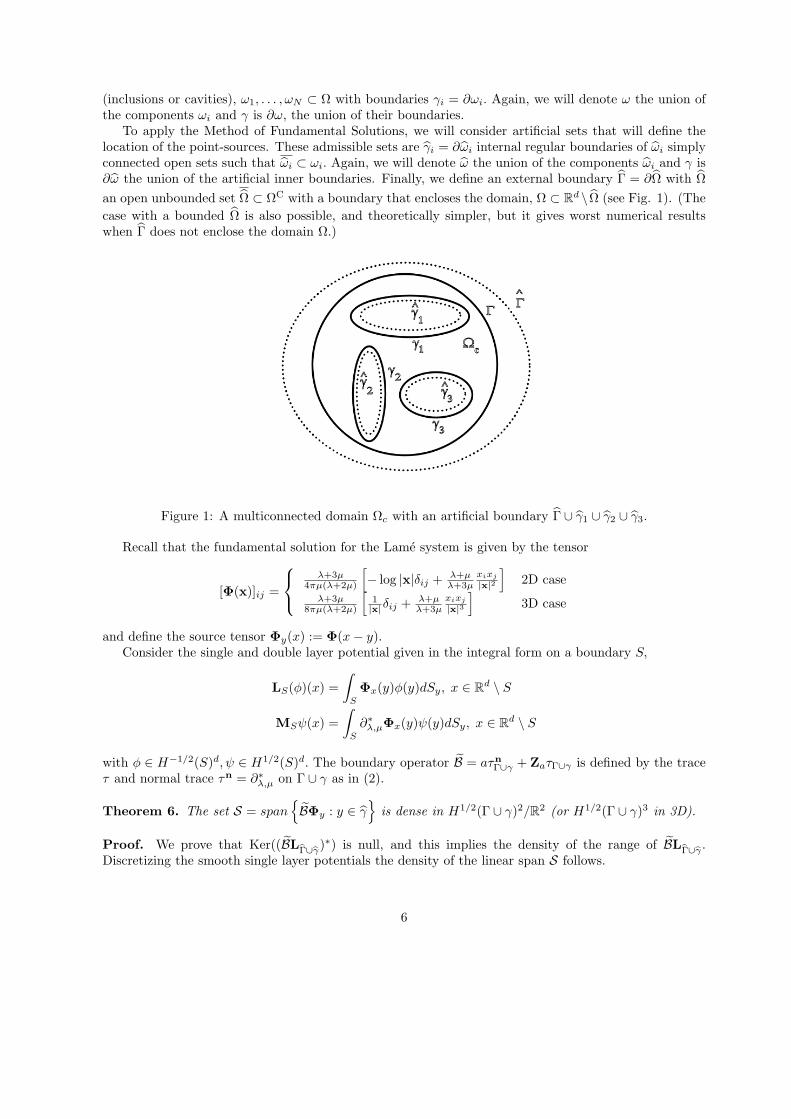
To apply the Method of Fundamental Solutions, we will consider artificial sets that will define thelocation of the point-sources. These admissible sets are γi = ∂ωi internal regular boundaries of ωi simplyconnected open sets such that ωi ⊂ ωi. Again, we will denote ω the union of the components ωi and γ is∂ω the union of the artificial inner boundaries. Finally, we define an external boundary Γ = ∂Ω with Ωan open unbounded set Ω ⊂ ΩC with a boundary that encloses the domain, Ω ⊂ Rd \ Ω (see Fig. 1). (Thecase with a bounded Ω is also possible, and theoretically simpler, but it gives worst numerical resultswhen Γ does not enclose the domain Ω.)

Figure 1: A multiconnected domain Ωc with an artificial boundary Γ ∪ γ1 ∪ γ2 ∪ γ3.

Recall that the fundamental solution for the Lame system is given by the tensor

[Φ(x)]ij =

λ+3µ4πµ(λ+2µ)

[− log |x|δij + λ+µ

λ+3µxixj

|x|2]

2D caseλ+3µ

8πµ(λ+2µ)

[1|x|δij + λ+µ

λ+3µxixj

|x|3]

3D case

and define the source tensor Φy(x) := Φ(x− y).Consider the single and double layer potential given in the integral form on a boundary S,

LS(φ)(x) =∫

S

Φx(y)φ(y)dSy, x ∈ Rd \ S

MSψ(x) =∫

S

∂∗λ,µΦx(y)ψ(y)dSy, x ∈ Rd \ S

with φ ∈ H−1/2(S)d, ψ ∈ H1/2(S)d. The boundary operator B = aτnΓ∪γ + ZaτΓ∪γ is defined by the trace

τ and normal trace τn = ∂∗λ,µ on Γ ∪ γ as in (2).

Theorem 6. The set S = spanBΦy : y ∈ γ

is dense in H1/2(Γ ∪ γ)2/R2 (or H1/2(Γ ∪ γ)3 in 3D).

Proof. We prove that Ker((BLΓ∪γ)∗) is null, and this implies the density of the range of BLΓ∪γ .Discretizing the smooth single layer potentials the density of the linear span S follows.

6

In 2D we consider

HZ(Γ ∪ γ) =

φ ∈ H1/2(Γ ∪ γ)2 :∫

Γ∪γ

Za(x)φ(x)dSx = 0

,

which can be identified to H1/2(Γ ∪ γ)2/Rp by taking a representative φ + C, defined by(∫

Γ∪γ

Za

)C =

∫

Γ∪γ

Zaφ,

being p the codimension of the matrix∫Γ∪γ

Za.

First, we note that (BLΓ∪γ)∗ = τΓ∪γ(aMΓ∪γ+τΓ∪γLΓ∪γZa), because⟨BLΓ∪γφ, ψ

⟩Γ∪γ

=⟨(aτn

Γ∪γLΓ∪γ+ZaτΓ∪γLΓ∪γ)φ, ψ⟩

Γ∪γ

=∫

Γ∪γ

(a∂∗λ,µ + Za(x)

) ∫

Γ∪γ

Φy(x)φ(y)dSyψ(x)dSx

=∫

Γ∪γ

∫

Γ∪γ

(a∂∗λ,µ + Za(x)

)Φy(x)ψ(x)dSxφ(y)dSy

=⟨aMΓ∪γψ + LΓ∪γZaψ, φ

⟩Γ∪γ

.

Now, let ψ ∈ HZ(Γ ∪ γ) (2D case) or ψ ∈ H1/2(Γ ∪ γ)3 (3D case) and define the analytic function

u(y) = (aMΓ∪γψ + LΓ∪γZaψ)(y), (y ∈ Rd \ (Γ ∪ γ)).

then (BLΓ∪γ)∗ψ = 0 is equivalent to u ≡ 0 on Γ ∪ γ. On the other hand, u verifies the Lame systemoutside Γ ∪ γ.

– Thus, u is the solution of the well posed exterior problem (cf. [11])

∆∗λ,µu = 0 in Ω

u = 0 on Γ

u(y) =

log |y| aZ +O(1) if d = 2O(|y|−1) if d = 3 |y| → ∞

and uniqueness implies u = 0 in Ω. In the 2D case, the uniqueness follows by taking the asymptoticbehavior with constant

aZ =λ + 3µ

4πµ(λ + 2µ)

∫

Γ∪γ

Za(x)φ(x)dSx,

hence aZ = 0 because φ ∈ HZ(Γ ∪ γ). In 3D the asymptotic behavior is immediately verified by thefundamental solution.By analytic continuation u = 0 in Ω implies u null in ΩC and the exterior traces u|+Γ , ∂∗λ,µu|+Γ are null.On the other hand, since

u(y) =∫

Γ∪γ

a ∂∗λ,µΦy(x)φ(x)dSx +∫

Γ∪γ

Za(x)Φy(x)φ(x)dSx

the boundary jumps on Γ are given by [u]Γ = −a φ|Γ ∧ [∂∗λ,µu]Γ = Zaφ|Γ and we conclude that

u|−Γ = −a φ|Γ ∧ ∂∗λ,µu|−Γ = Zaφ|Γ .

7

– Also, u is the solution of the well posed interior problems for each j = 1, . . . , N ,

∆∗λ,µu = 0 in ωj

u = 0 on γj

hence, u = 0 in ωj . Again, by analytic continuation this implies u = 0 in each ωj and the exterior tracesu|+γj

, ∂∗λ,µu|+γjare null, thus

u|−γj= −a φ|γj

∧ ∂∗λ,µu|−γj= Za φ|−γj

on γj .

Therefore, u is also a solution of the interior problem

∆∗λ,µu

− = 0 in Ωc

a ∂∗λ,µu− + Zau− = 0 on ∂Ωc = Γ ∪ γ

and by the well posedness of this problem we have u− = 0 in Ωc. This implies that all traces u|−Γ∪γ and∂∗λ,µu|−Γ∪γ are null and, on the whole Γ ∪ γ,

a φ = [u] = 0 ∧ Zaφ = [∂∗λ,µu] = 0

this implies φ = 0, from the restrictions on a, Za. ¤

We now address the question of solving the direct problem (PΩc) with the MFS.

Consider the solution of (PΩc) represented by the single layer potential that we separate into a sum

u = LΓ∪γψ = LΓψ|Γ + Lγψ|γ . (6)

On the boundary Γ ∪ γ we also separate the integral equations

BΓLΓ∪γψ = g, BγLΓ∪γψ = 0 (7)

with g ∈ H1/2(Γ)d. This leads to a matrix operator system[BΓLΓ BΓLγ

BγLΓ BγLγ

]

︸ ︷︷ ︸M(Γ,γ)

[ψ|Γψ|γ

]=

[g0

]. (8)

The MFS consists in using the approximation justified by the density result

u(x) = LΓ∪γψ(x) ≈n∑

i=1

αiΦyi(x) =: u(x)

for some source points y1, . . . , yn ∈ Γ ∪ γ. We then compute the vectorial coefficients αi = (αi,1, αi,2) bysolving the linear system

Φy1(x1) . . . Φyn(x1). . . . . . . . .

Φy1(xl) . . . Φyn(xl)Φy1(xl+1) . . . Φyn(xl+1)

. . . . . . . . .Φy1(xm) . . . Φyn(xm)

α1

...αn

=

g(x1)...

g(xl)0...0

(9)

on some collocation points x1, . . . , xl ∈ Γ and xl+1, . . . , xm ∈ γ (l < m).

8

3.2 MFS version of the KKM

We now consider the inverse problem, ie., to obtain the shape of the boundary γ from the Cauchy dataon Γ and will assume that BΓ is the Dirichlet boundary operator on Γ. The Kirsch-Kress Method (cf.[17]) was initially presented for acoustic scattering (twenty years ago), and the external boundary Γ wasthen replaced by the knowledge of the far field pattern.

The method consists in assuming that some knowledge on γ exists, such that we can prescribe anartificial boundary γ inside γ and write the solution in terms of the inner boundary layer representation.

In the acoustic scattering problem the unknown density for the artificial inner boundary layer wasrecovered fitting its far field pattern. In the bounded domain we need to fit the Cauchy data and it isclear that the inner boundary will not be enough to adjust both Dirichlet and Neumann data. An extraexternal boundary layer must be considered.

At least two adaptations could be possible for the bounded domain:(a) Use the boundary element method (BEM) formulation, and the extra boundary layer would be

defined on the external accessible boundary Γ.(b) Use the method of fundamental solutions (MFS) and define an external artificial boundary layer

Γ.

We will consider the second approach, and therefore it should be considered that we will use the MFSadaptation of the Kirsch-Kress Method (KKM).

Therefore the MFS version of the KKM method for the inverse bounded problem consists in two steps:

(i) linear part: solving the system of integral equations[

τΓLΓ τΓLγ

τnΓ LΓ τn

Γ Lγ

]

︸ ︷︷ ︸K(Γ,Γ)

[φ|Γφ|γ

]=

[g

∂∗λ,µu

], (10)

where τΓ, τnΓ are, respectively the trace and the normal trace on Γ.

Note that K(Γ, Γ) is M(Γ, Γ) with BΓ = τΓ and Bγ = τnΓ , when γ = Γ.

(ii) nonlinear part: the boundary γ will be given by the level set u−1(0) = x ∈ Ω : u(x) = 0, for theDirichlet problem (or computed iteratively, in an optimization scheme for a class of approximatingshapes, for the Neumann or other boundary condition).

The linear part of the Kirsch-Kress Method to solve the Cauchy problem is therefore connected tothe MFS since it may use the same boundary layers on γ and on Γ to give the solution of the directproblem from the Dirichlet boundary conditions on γ and Γ, and the reconstruction of the solution fromthe Dirichlet and Neumann data on Γ. In fact, the first line of the system (10) would be the same –known Dirichlet data. The same densities φ|Γ and φ|γ will verify both systems (8) and (10).

We now prove that a pair of Cauchy data can be retrieved using this MFS version of the KKM method.

Theorem 7. The setSn = span

(τΓΦy, τn

Γ Φy) : y ∈ Γ ∪ γ

is dense in H1/2(Γ)2/R2 ×H−1/2(Γ)2 (or H1/2(Γ)3 ×H−1/2(Γ)3 in 3D).

Proof. We follow the proof of Theorem 6. The adjoint of the matrix operator K(Γ, Γ) defined in (10) isgiven by

K(Γ, Γ)∗ =[

τΓLΓ τΓLγ

τnΓ LΓ τn

Γ Lγ

]∗=

[τΓLΓ τΓMΓ

τΓLγ τγMΓ

].

9

In the 2D case, again the space HI(Γ) is identified to H1/2(Γ)2/R2 (taking the representativeφ− 1

|Γ|∫Γ

φ ).Let φ ∈ HI(Γ), ψ ∈ H−1/2(Γ)2 (2D case) or φ ∈ H1/2(Γ)3, ψ ∈ H−1/2(Γ)3 (3D case) and define the

functionu(y) = (LΓφ)(y) + (MΓψ)(y)

a combination of single and double layer potentials defined on Γ. Following the same arguments, as inTheorem 6, we prove that if u = 0 on Γ ∪ γ then by analytic continuation of the unique null solution ofthe interior and exterior problems (now aZ = λ+3µ

4πµ(λ+2µ)

∫Γ

φ(x)dSx = 0, because φ ∈ HI(Γ)), we obtainu = 0 in Rd \ Γ. Then φ = [∂∗λ,µu]

Γ= 0 and ψ = −[u]Γ= 0. and the result follows. ¤

4 Numerical Simulations

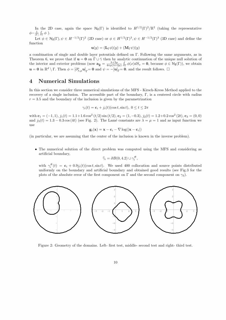
In this section we consider three numerical simulations of the MFS - Kirsch-Kress Method applied to therecovery of a single inclusion. The accessible part of the boundary, Γ, is a centered circle with radiusr = 3.5 and the boundary of the inclusion is given by the parametrization

γi(t) = ci + ji(t)(cos t, sin t), 0 ≤ t ≤ 2π

with c1 = (−1, 1), j1(t) = 1.1+1.6 cos2 (t/2) sin (t/2), c2 = (1,−0.3), j2(t) = 1.2+0.2 cos2 (2t), c3 = (0, 0)and j3(t) = 1.3 − 0.3 cos (4t) (see Fig. 2). The Lame constants are λ = µ = 1 and as input function weuse

gi(x) = x− ci −∇ log(|x− ci|)(in particular, we are assuming that the center of the inclusion is known in the inverse problem).

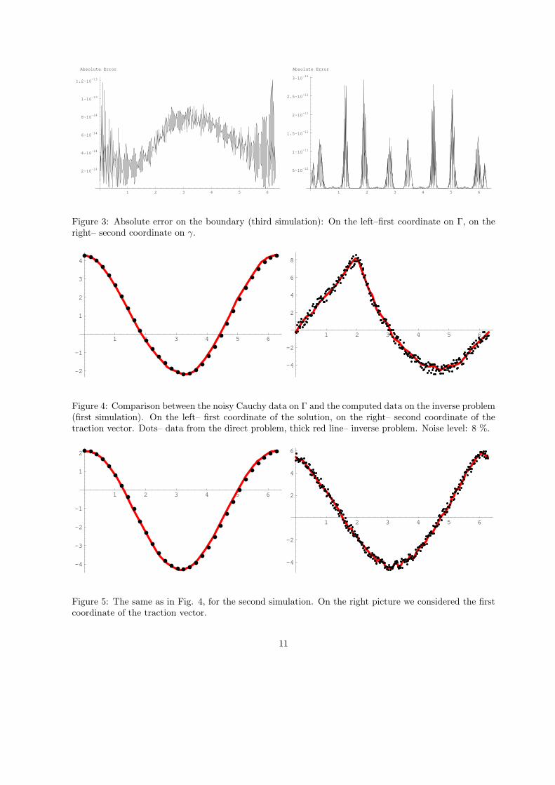
• The numerical solution of the direct problem was computed using the MFS and considering asartificial boundary,

γi = ∂B(0, 4.2) ∪ γ#i ,

with γ#i (t) = ci + 0.9ji(t)(cos t, sin t). We used 400 collocation and source points distributed

uniformly on the boundary and artificial boundary and obtained good results (see Fig.3 for theplots of the absolute error of the first component on Γ and the second component on γ3).

-3 -2 -1 1 2 3

-3

-2

-1

1

2

3

-3 -2 -1 1 2 3

-3

-2

-1

1

2

3

-3 -2 -1 1 2 3

-3

-2

-1

1

2

3

Figure 2: Geometry of the domains. Left- first test, middle- second test and right- third test.

10

1 2 3 4 5 6

2·10-14

4·10-14

6·10-14

8·10-14

1·10-13

1.2·10-13

Absolute Error

1 2 3 4 5 6

5·10-12

1·10-11

1.5·10-11

2·10-11

2.5·10-11

3·10-11

Absolute Error

Figure 3: Absolute error on the boundary (third simulation): On the left–first coordinate on Γ, on theright– second coordinate on γ.

1 2 3 4 5 6

-2

-1

1

2

3

4

1 2 3 4 5 6

-4

-2

2

4

6

8

Figure 4: Comparison between the noisy Cauchy data on Γ and the computed data on the inverse problem(first simulation). On the left– first coordinate of the solution, on the right– second coordinate of thetraction vector. Dots– data from the direct problem, thick red line– inverse problem. Noise level: 8 %.

1 2 3 4 5 6

-4

-3

-2

-1

1

2

1 2 3 4 5 6

-4

-2

2

4

6

Figure 5: The same as in Fig. 4, for the second simulation. On the right picture we considered the firstcoordinate of the traction vector.

11

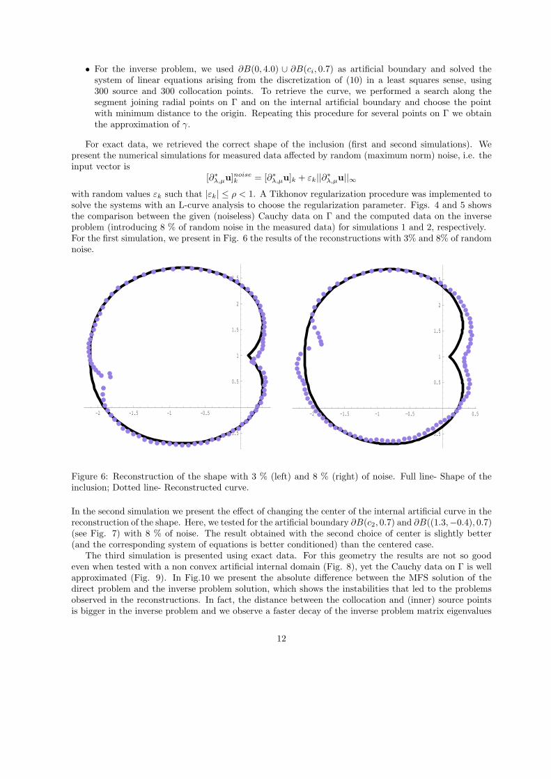
• For the inverse problem, we used ∂B(0, 4.0) ∪ ∂B(ci, 0.7) as artificial boundary and solved thesystem of linear equations arising from the discretization of (10) in a least squares sense, using300 source and 300 collocation points. To retrieve the curve, we performed a search along thesegment joining radial points on Γ and on the internal artificial boundary and choose the pointwith minimum distance to the origin. Repeating this procedure for several points on Γ we obtainthe approximation of γ.

For exact data, we retrieved the correct shape of the inclusion (first and second simulations). Wepresent the numerical simulations for measured data affected by random (maximum norm) noise, i.e. theinput vector is

[∂∗λ,µu]noisek = [∂∗λ,µu]k + εk||∂∗λ,µu||∞

with random values εk such that |εk| ≤ ρ < 1. A Tikhonov regularization procedure was implemented tosolve the systems with an L-curve analysis to choose the regularization parameter. Figs. 4 and 5 showsthe comparison between the given (noiseless) Cauchy data on Γ and the computed data on the inverseproblem (introducing 8 % of random noise in the measured data) for simulations 1 and 2, respectively.For the first simulation, we present in Fig. 6 the results of the reconstructions with 3% and 8% of randomnoise.

-2 -1.5 -1 -0.5

-0.5

0.5

1

1.5

2

2.5

-2 -1.5 -1 -0.5 0.5

-0.5

0.5

1

1.5

2

2.5

Figure 6: Reconstruction of the shape with 3 % (left) and 8 % (right) of noise. Full line- Shape of theinclusion; Dotted line- Reconstructed curve.

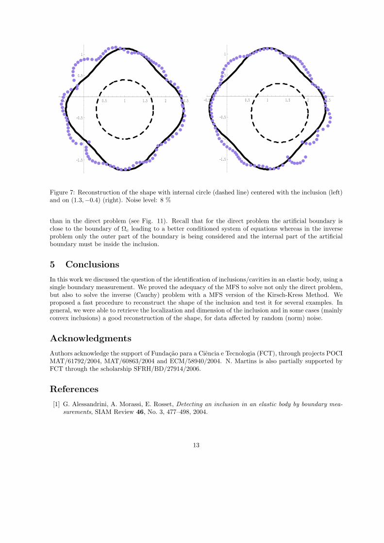
In the second simulation we present the effect of changing the center of the internal artificial curve in thereconstruction of the shape. Here, we tested for the artificial boundary ∂B(c2, 0.7) and ∂B((1.3,−0.4), 0.7)(see Fig. 7) with 8 % of noise. The result obtained with the second choice of center is slightly better(and the corresponding system of equations is better conditioned) than the centered case.

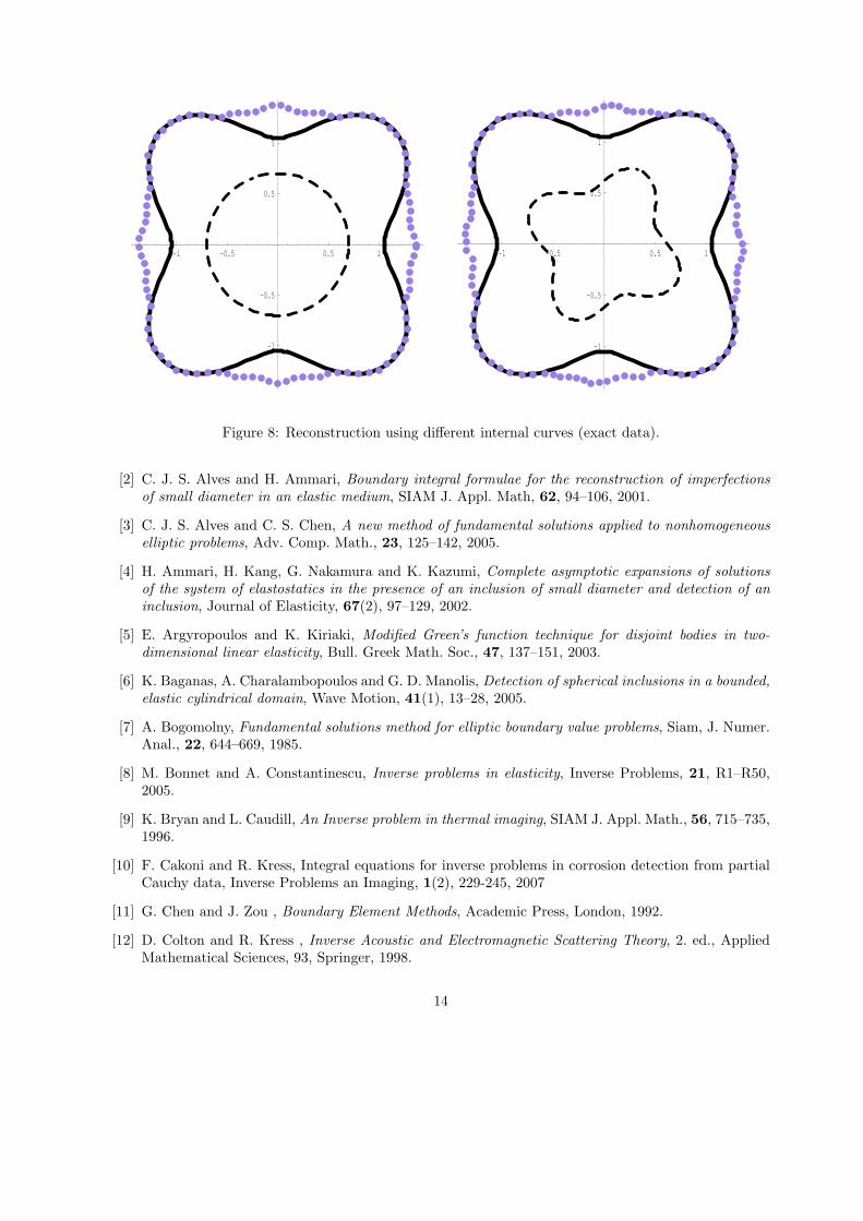
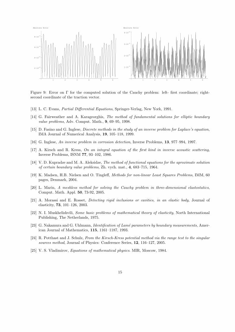
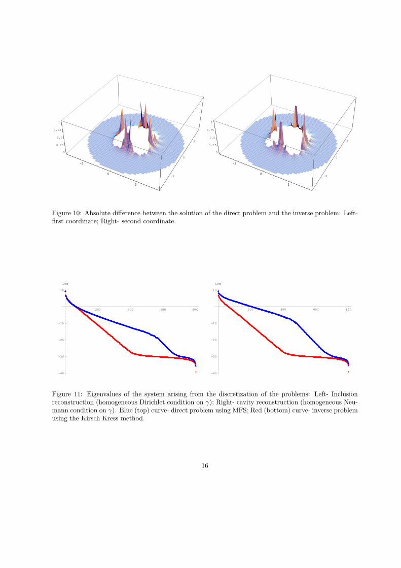
The third simulation is presented using exact data. For this geometry the results are not so goodeven when tested with a non convex artificial internal domain (Fig. 8), yet the Cauchy data on Γ is wellapproximated (Fig. 9). In Fig.10 we present the absolute difference between the MFS solution of thedirect problem and the inverse problem solution, which shows the instabilities that led to the problemsobserved in the reconstructions. In fact, the distance between the collocation and (inner) source pointsis bigger in the inverse problem and we observe a faster decay of the inverse problem matrix eigenvalues

12

-0.5 0.5 1 1.5 2 2.5

-1.5

-1

-0.5

0.5

1

-0.5 0.5 1 1.5 2 2.5

-1.5

-1

-0.5

0.5

1

Figure 7: Reconstruction of the shape with internal circle (dashed line) centered with the inclusion (left)and on (1.3,−0.4) (right). Noise level: 8 %

than in the direct problem (see Fig. 11). Recall that for the direct problem the artificial boundary isclose to the boundary of Ωc leading to a better conditioned system of equations whereas in the inverseproblem only the outer part of the boundary is being considered and the internal part of the artificialboundary must be inside the inclusion.

5 Conclusions

In this work we discussed the question of the identification of inclusions/cavities in an elastic body, using asingle boundary measurement. We proved the adequacy of the MFS to solve not only the direct problem,but also to solve the inverse (Cauchy) problem with a MFS version of the Kirsch-Kress Method. Weproposed a fast procedure to reconstruct the shape of the inclusion and test it for several examples. Ingeneral, we were able to retrieve the localization and dimension of the inclusion and in some cases (mainlyconvex inclusions) a good reconstruction of the shape, for data affected by random (norm) noise.

Acknowledgments

Authors acknowledge the support of Fundacao para a Ciencia e Tecnologia (FCT), through projects POCIMAT/61792/2004, MAT/60863/2004 and ECM/58940/2004. N. Martins is also partially supported byFCT through the scholarship SFRH/BD/27914/2006.

References

[1] G. Alessandrini, A. Morassi, E. Rosset, Detecting an inclusion in an elastic body by boundary mea-surements, SIAM Review 46, No. 3, 477–498, 2004.

13

-1 -0.5 0.5 1

-1

-0.5

0.5

1

-1 -0.5 0.5 1

-1

-0.5

0.5

1

Figure 8: Reconstruction using different internal curves (exact data).

[2] C. J. S. Alves and H. Ammari, Boundary integral formulae for the reconstruction of imperfectionsof small diameter in an elastic medium, SIAM J. Appl. Math, 62, 94–106, 2001.

[3] C. J. S. Alves and C. S. Chen, A new method of fundamental solutions applied to nonhomogeneouselliptic problems, Adv. Comp. Math., 23, 125–142, 2005.

[4] H. Ammari, H. Kang, G. Nakamura and K. Kazumi, Complete asymptotic expansions of solutionsof the system of elastostatics in the presence of an inclusion of small diameter and detection of aninclusion, Journal of Elasticity, 67(2), 97–129, 2002.

[5] E. Argyropoulos and K. Kiriaki, Modified Green’s function technique for disjoint bodies in two-dimensional linear elasticity, Bull. Greek Math. Soc., 47, 137–151, 2003.

[6] K. Baganas, A. Charalambopoulos and G. D. Manolis, Detection of spherical inclusions in a bounded,elastic cylindrical domain, Wave Motion, 41(1), 13–28, 2005.

[7] A. Bogomolny, Fundamental solutions method for elliptic boundary value problems, Siam, J. Numer.Anal., 22, 644–669, 1985.

[8] M. Bonnet and A. Constantinescu, Inverse problems in elasticity, Inverse Problems, 21, R1–R50,2005.

[9] K. Bryan and L. Caudill, An Inverse problem in thermal imaging, SIAM J. Appl. Math., 56, 715–735,1996.

[10] F. Cakoni and R. Kress, Integral equations for inverse problems in corrosion detection from partialCauchy data, Inverse Problems an Imaging, 1(2), 229-245, 2007

[11] G. Chen and J. Zou , Boundary Element Methods, Academic Press, London, 1992.

[12] D. Colton and R. Kress , Inverse Acoustic and Electromagnetic Scattering Theory, 2. ed., AppliedMathematical Sciences, 93, Springer, 1998.

14

1 2 3 4 5 6

2·10-9

4·10-9

6·10-9

8·10-9

Absolute Error

1 2 3 4 5 6

1·10-9

2·10-9

3·10-9

4·10-9

Absolute Error

Figure 9: Error on Γ for the computed solution of the Cauchy problem: left- first coordinate; right-second coordinate of the traction vector.

[13] L. C. Evans, Partial Differential Equations, Springer-Verlag, New York, 1991.

[14] G. Fairweather and A. Karageorghis, The method of fundamental solutions for elliptic boundaryvalue problems, Adv. Comput. Math., 9, 69–95, 1998.

[15] D. Fasino and G. Inglese, Discrete methods in the study of an inverse problem for Laplace’s equation,IMA Journal of Numerical Analysis, 19, 105–118, 1999.

[16] G. Inglese, An inverse problem in corrosion detection, Inverse Problems, 13, 977–994, 1997.

[17] A. Kirsch and R. Kress, On an integral equation of the first kind in inverse acoustic scattering,Inverse Problems, ISNM 77, 93–102, 1986.

[18] V. D. Kupradze and M. A. Aleksidze, The method of functional equations for the aproximate solutionof certain boundary value problems, Zh. vych. mat., 4, 683–715, 1964.

[19] K. Madsen, H.B. Nielsen and O. Tingleff, Methods for non-linear Least Squares Problems, IMM, 60pages, Denmark, 2004.

[20] L. Marin, A meshless method for solving the Cauchy problem in three-dimensional elastostatics,Comput. Math. Appl. 50, 73-92, 2005.

[21] A. Morassi and E. Rosset, Detecting rigid inclusions or cavities, in an elastic body, Journal ofelasticity, 73, 101–126, 2003.

[22] N. I. Muskhelishvili, Some basic problems of mathematical theory of elasticity, North InternationalPublishing, The Netherlands, 1975.

[23] G. Nakamura and G. Uhlmann, Identification of Lame parameters by boundary measurements, Amer-ican Journal of Mathematics, 115, 1161–1187, 1993.

[24] R. Potthast and J. Schulz, From the Kirsch-Kress potential method via the range test to the singularsources method, Journal of Physics: Conference Series, 12, 116–127, 2005.

[25] V. S. Vladimirov, Equations of mathematical physics. MIR, Moscow, 1984.

15

-2

0

2

-2

0

2

0

0.25

0.5

0.75

1

-2

0

2

-2

0

2

-2

0

2

0

0.25

0.5

0.75

1

-2

0

2

Figure 10: Absolute difference between the solution of the direct problem and the inverse problem: Left-first coordinate; Right- second coordinate.

200 400 600 800

-40

-30

-20

-10

10

Log

200 400 600 800

-40

-30

-20

-10

10

Log

Figure 11: Eigenvalues of the system arising from the discretization of the problems: Left- Inclusionreconstruction (homogeneous Dirichlet condition on γ); Right- cavity reconstruction (homogeneous Neu-mann condition on γ). Blue (top) curve- direct problem using MFS; Red (bottom) curve- inverse problemusing the Kirsch Kress method.

16