Embed Size (px)
Citation preview
General rights Copyright and moral rights for the publications made accessible in the public portal are retained by the authors and/or other copyright owners and it is a condition of accessing publications that users recognise and abide by the legal requirements associated with these rights.
Users may download and print one copy of any publication from the public portal for the purpose of private study or research.
You may not further distribute the material or use it for any profit-making activity or commercial gain
You may freely distribute the URL identifying the publication in the public portal If you believe that this document breaches copyright please contact us providing details, and we will remove access to the work immediately and investigate your claim.
Downloaded from orbit.dtu.dk on: Dec 27, 2019
The direct Flow parametric Proof of Gauss' Divergence Theorem revisited
Markvorsen, Steen
Publication date:2006
Document VersionEarly version, also known as pre-print
Link back to DTU Orbit
Citation (APA):Markvorsen, S. (2006). The direct Flow parametric Proof of Gauss' Divergence Theorem revisited. Departmentof Mathematics, Technical University of Denmark. Mat-Report, No. 2006-15
THE DIRECT FLOW PARAMETRIC PROOF OFGAUSS’ DIVERGENCE THEOREM REVISITED
STEEN MARKVORSEN
Abstract. The standard proof of the divergence theorem in un-dergraduate calculus courses covers the theorem for static domainsbetween two graph surfaces. We show that within first year un-dergraduate curriculum, the flow proof of the dynamic version ofthe divergence theorem - which is usually considered only muchlater in more advanced math courses - is comprehensible with onlya little extension of the first year curriculum. Moreover, it is moreintuitive than the static proof. We support this intuition furtherby unfolding and visualizing a few examples with increasing com-plexity. In these examples we apply the key instrumental conceptsand verify the various steps towards this alternative proof of thedivergence theorem.
1. Introduction
With the advent and aid of modern tools for visualizations and calcu-lations, the study of integral curves of vector fields in space has becomemuch more accessible and comprehensible. It is now an easy matterto simulate flows along given vector fields in 3D and thence visualizethe corresponding deformation of curves, surfaces and bodies floatingalong with the flow.
Here we think of the flow deformation of a given geometric object asbeing organized so that each point of the object follows its own deter-mined flow line so that the full object is pushed forward and at the sametime deformed by the flow map in the direction of the given vector field.
Intuition concerning the flow map is thereby firmly developed andsupported. Several first rate questions emerge naturally among stu-dents when seeing this deformation take place in, say, a 3D animation:How much is this curve elongated during the flow? What is the totaldeformation of that surface? Why does’nt it self-intersect during theflow? What is the volume of a compact floating body after time t?
2000 Mathematics Subject Classification. Primary 26.Key words and phrases. Gauss’ divergence theorem in 3D, vector fields, integral
curves, flow map, push forward map, curriculum, visualization, process orientedlearning.
1
2 S. MARKVORSEN
The answers to these questions are all contained in (the flow proofof) Gauss’ divergence theorem which we now state in its full dynamicgenerality for compact domains and vector fields in 3D:
Theorem 1.1 (Gauss’ divergence theorem, flow version). Let Ω0 de-note a compact domain in R3 with piecewise smooth boundary ∂Ω0 andoutward pointing unit normal vector field n∂Ω0 on ∂Ω0. Let V be avector field in R3 with corresponding flow map Ft. Let Ωt = Ft(Ω0).Then
(1.1)
(d
dt
)
|t=0
Vol(Ωt) =
∫
Ω0
div(V) dµ =
∫
∂Ω0
V · n∂Ω0 dν .
The flow map Ft will be defined in detail via the examples belowand in Theorem 2.5.
The right hand side of (1.1) is the outwards directed flux of the vec-tor field through the boundary of the domain.
Of course, along the way of proving Theorem 1.1 we must expect andanswer yet another pertinent and natural question from the students:What is the precise role of the divergence in this statement? How doesthis emerge from the action of the flow map?
Before entering into the details of answering these questions and pro-ving the theorem, we make a few remarks concerning the developmentof the theorem, i.e. concerning its origin and history and concerningits momentum within standard first year curriculum.
Gauss’ divergence theorem is of the same calibre as Stokes’ theorem.They are both members of a family of results which are concerned with’pushing the integration to the boundary’. The eldest member of thisfamily is the following:
Theorem 1.2 (Fundamental theorem of calculus). Let f be a conti-nuous function on R. Then the function
A(x) =
∫ x
0
f(u) du
is differentiable with
(1.2) A′(x) = f(x) ,
and moreover, if F (x) is any (other) function satisfying F ′(x) = f(x),then
(1.3)
∫ b
a
f(u) du = F (b)− F (a) .
GAUSS’ DIVERGENCE THEOREM REVISITED 3
The message of this theorem is that two fundamental problems - thatof finding a function whose derivative is a given function and that offinding the average of a given function - have a common solution. It isalso the first result which displays - in equation (1.3) - the astoundingsuccess of ’pushing the integration to the boundary’.
The divergence theorem is not - conceptually speaking - ’far’ fromthe fundamental theorem of calculus. Most textbook proofs of the di-vergence theorem covers only the special setting of a static domainwhose boundary consists of the graphs of two functions, each of twovariables. This enables in fact a direct proof in this special case viaTheorem 1.2, see [EP] pp. 1058–1059. Stokes’ theorem is a little harderto grasp, even locally, but follows also in the corresponding setting (forgraph surfaces) from Gauss’ theorem for planar domains, see [EP] pp.1065–1066. Stokes’ theorem can alternatively be presented in the samevein as the divergence theorem is presented in this paper. One versionof such a proof can be found in [Mar].
The idea of unfolding the details of Gauss’ divergence theorem inthis generality via a flow parametric proof on the platform of firstyear undergraduate curriculum has - to the best of the present authorsknowledge - not yet been implemented in any calculus book. We mustmention, however, that the dynamic version of the divergence theoremin two dimensions has been covered in a similar vein via an applicationof the co-area formula in the recent beautiful paper [ES] by Eisenbergand Sullivan.
Among the many interesting efforts to improve the teaching of vectorcalculus in general - and of its applications, in particular to electro-magnetism - we also refer to [FLS], [She], [A], [DuB] and [DoB]. Theseefforts are typically initiated from the community of physics teachers.However, as expressed clearly in [DuB] there is room for - as well as aneed for - a fruitful dialogue with the mathematics teachers concerningthese issues.
The main purpose of the present work is in this spirit to try and fa-cilitate the first presentation, i.e. the undergraduate teaching, as wellas the general intuition of the divergence theorem and thus to prepareit for later use in the applied fields.
The presentation is ’compatible’ with the Worldwide calculus cur-riculum in the sense that throughout this paper we make explicit use ofvector parametrizations of surfaces and curves and their correspondingJacobian functions. This gives maximal flexibility for choosing con-crete examples and illustrations, not only for the divergence theorem
4 S. MARKVORSEN
itself, but also for each step in the proof as will be indicated by threeexamples in the present paper.
What may be new in comparison with the typical first year cur-riculum is the necessary tools and results from systems of differentialequations and their solutions. At the Technical University of Denmarkwe have successfully chosen to introduce 2 × 2 linear ODE systemsand their complete solutions (via eigen-solutions of the system matrix)into the first semester curriculum. This gives in particular a wonderfulapplication of linear algebra to establish existence and uniqueness ofsolutions in these simplest (linear, planar) cases. The step to 3 × 3linear ODE systems is then not a difficult one. The step to non-linear3× 3 systems is, of course, the real hurdle but conceptually still withinreach - in particular with the advent and aid of modern computer fa-cilities.
Finally, concerning the history of the divergence theorem, one inte-resting account is given by Crowe in [C], from where we quote:
The history of these theorems [Green’s, Stokes’, andGauss’ theorems] has never (to my knowledge) beenwritten. It essentially lies outside the history of vec-tor analysis, for the theorems were all developed orig-inally for Cartesian analysis, and by people who didnot work with vectors. Some comments may howeverbe made. Gauss’ Theorem (often called the DivergenceTheorem) is attributed (by Hermann Rothe [1931?]) toGauss [1840].
James Clerk Maxwell [ in his Treatise on Electricityand Magnetism ] stated that Gauss’ Theorem ”... seemsto have been first given by Ostrogradsky in a paper readin 1828, but published in 1831 [...]”. This note is notcontained in the first edition of his Treatise [1891]. Thisfact is doubly interesting as possibly indicating whereMaxwell first found the theorem.
Oliver Dimon Kellogg, Foundations of Potential The-ory [1953] wrote the following in regard to Gauss’ The-orem: ”A similar reduction of triple integrals to doubleintegrals was employed by Lagrange [1760]. The doubleintegrals are given in more definite form by Gauss [1813].A systematic use of integral identities equivalent to thedivergence theorem was made by George Green in hisEssay on the Application of Mathematical Analysis tothe Theory of Electricity and Magnetism, Nottingham,1828.”
M. J. Crowe, [C] p. 146.
GAUSS’ DIVERGENCE THEOREM REVISITED 5
Acknowledgement . This work was carried out while the author waspart time affiliated with the Learning Lab DTU. The author wouldlike to thank the staff and colleagues at the Learning Lab DTU forkind hospitality, for rewarding and inspiring discussions on curriculum,teaching, and learning, and for technical and financial support.
Outline of paper . In section 2 we consider and illustrate, mainly byexamples, the flow maps associated to given vector fields. The proofof the divergence theorem is orchestrated in sections 3, 4, and 5. Thecovariant (directional) derivative of a vector field is applied in section3 to give precise information about the deformation of curves. Thet−derivative of the volume of a floating domain can then be expressedin two ways: An ’intrinsic’ calculation gives rise to the divergence in-tegral (section 4), and an ’extrinsic’ calculation gives rise to the fluxintegral (section 5).
2. The flow of a vector field
A smooth parametrized curve γ(t) in R3 has a tangent vector fieldγ ′(t) along the curve. The curve is an integral curve for a given vectorfield V if the tangent vector at every point of the curve is preciselythe given vector field evaluated at that point. The integral curves aretherefore solutions to the following differential equation:
γ ′(t) = V(γ(t)) .
In cartesian coordinates in R3 we have
γ(t) = (x(t), y(t), z(t)) ,
γ ′(t) = (x′(t), y′(t), z′(t)) and
V(x, y, z) = (V1(x, y, z), V2(x, y, z), V3(x, y, z)) .
The system of ordinary differential equations corresponding to the vec-tor equation γ ′(t) = V(γ(t)) is thus
(2.1)
x′(t) = V1(x(t), y(t), z(t))
y′(t) = V2(x(t), y(t), z(t))
z′(t) = V3(x(t), y(t), z(t)) .
The integral curve through a given point (x0, y0, z0) is obtained byusing this point as the initial condition for the system of differentialequations.
We present 3 examples with slightly increasing complexity, but al-ways with emphasis on different elementary aspects of the theory.
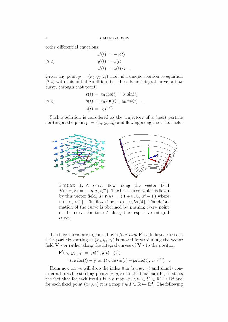
Example 2.1. The vector field in Figure 1, V(x, y, z) = (−y, x, z/7)has integral curves defined by the following system of ordinary first
6 S. MARKVORSEN
order differential equations:
(2.2)
x′(t) = −y(t)
y′(t) = x(t)
z′(t) = z(t)/7 .
Given any point p = (x0, y0, z0) there is a unique solution to equation(2.2) with this initial condition, i.e. there is an integral curve, a flowcurve, through that point:
(2.3)
x(t) = x0 cos(t)− y0 sin(t)
y(t) = x0 sin(t) + y0 cos(t)
z(t) = z0 et/7.
.
Such a solution is considered as the trajectory of a (test) particlestarting at the point p = (x0, y0, z0) and flowing along the vector field.
y
z
x
y
z
Figure 1. A curve flow along the vector fieldV(x, y, z) = (−y, x, z/7). The base curve, which is flownby this vector field, is: r(u) = ( 1 + u, 0, u2 − 1 ) whereu ∈ [ 0,
√2 ]. The flow time is t ∈ [ 0, 5π/4 ]. The defor-
mation of the curve is obtained by pushing every pointof the curve for time t along the respective integralcurves.
The flow curves are organized by a flow map Ft as follows. For eacht the particle starting at (x0, y0, z0) is moved forward along the vectorfield V - or rather along the integral curves of V - to the position
Ft(x0, y0, z0) = (x(t), y(t), z(t))
= (x0 cos(t)− y0 sin(t), x0 sin(t) + y0 cos(t), z0 et/7) .
From now on we will drop the index 0 in (x0, y0, z0) and simply con-sider all possible starting points (x, y, z) for the flow map Ft, to stressthe fact that for each fixed t it is a map (x, y, z) ∈ U ⊂ R3 7→ R3 andfor each fixed point (x, y, z) it is a map t ∈ I ⊂ R 7→ R3. The following
GAUSS’ DIVERGENCE THEOREM REVISITED 7
pertinent question emerges naturally: Given a time t, what is then themaximal set U = Mt for which the flow map is defined? And given apoint (x, y, z) what is then the maximal interval I = D(x,y,z) for whichthe flow map is defined? These maximal sets will be considered in theexamples and defined precisely below in Definition 2.2.
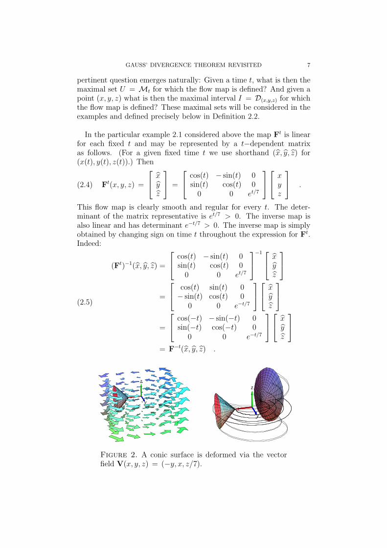
In the particular example 2.1 considered above the map Ft is linearfor each fixed t and may be represented by a t−dependent matrixas follows. (For a given fixed time t we use shorthand (x, y, z) for(x(t), y(t), z(t)).) Then
(2.4) Ft(x, y, z) =
xyz
=
cos(t) − sin(t) 0sin(t) cos(t) 0
0 0 et/7
xyz
.
This flow map is clearly smooth and regular for every t. The deter-minant of the matrix representative is et/7 > 0. The inverse map isalso linear and has determinant e−t/7 > 0. The inverse map is simplyobtained by changing sign on time t throughout the expression for Ft.Indeed:
(2.5)
(Ft)−1(x, y, z) =
cos(t) − sin(t) 0sin(t) cos(t) 0
0 0 et/7
−1
xyz
=
cos(t) sin(t) 0− sin(t) cos(t) 0
0 0 e−t/7
xyz
=
cos(−t) − sin(−t) 0sin(−t) cos(−t) 0
0 0 e−t/7
xyz
= F−t(x, y, z) .
y
z
y
z
Figure 2. A conic surface is deformed via the vectorfield V(x, y, z) = (−y, x, z/7).
8 S. MARKVORSEN
z
y
z
y
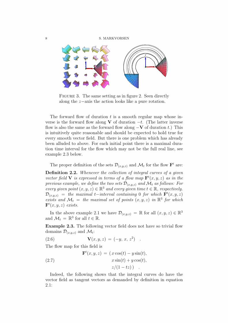
Figure 3. The same setting as in figure 2. Seen directlyalong the z−axis the action looks like a pure rotation.
The forward flow of duration t is a smooth regular map whose in-verse is the forward flow along V of duration −t. (The latter inverseflow is also the same as the forward flow along −V of duration t.) Thisis intuitively quite reasonable and should be expected to hold true forevery smooth vector field. But there is one problem which has alreadybeen alluded to above. For each initial point there is a maximal dura-tion time interval for the flow which may not be the full real line, seeexample 2.3 below.
The proper definition of the sets D(x,y,z) and Mt for the flow Ft are:
Definition 2.2. Whenever the collection of integral curves of a givenvector field V is expressed in terms of a flow map Ft(x, y, z) as in theprevious example, we define the two sets D(x,y,z) and Mt as follows: Forevery given point (x, y, z) ∈ R3 and every given time t ∈ R, respectively.D(x,y,z) = the maximal t−interval containing 0 for which Ft(x, y, z)exists and Mt = the maximal set of points (x, y, z) in R3 for whichFt(x, y, z) exists.
In the above example 2.1 we have D(x,y,z) = R for all (x, y, z) ∈ R3
and Mt = R3 for all t ∈ R.
Example 2.3. The following vector field does not have so trivial flowdomains D(x,y,z) and Mt:
(2.6) V(x, y, z) = (−y, x, z2) .
The flow map for this field is
(2.7)
Ft(x, y, z) = ( x cos(t)− y sin(t),
x sin(t) + y cos(t),
z/(1− tz) ) .
Indeed, the following shows that the integral curves do have thevector field as tangent vectors as demanded by definition in equation2.1:
GAUSS’ DIVERGENCE THEOREM REVISITED 9
(2.8)
∂
∂tFt(x, y, z) = (x′(t), y′(t), z′(t))
= (−y(t), x(t), z(t)2)
= V(x(t), y(t), z(t))
= V(Ft(x, y, z)) .
If z = 0 the flow map is defined for all values of t - the maximalflow-time interval is R for all the initial points lying in the z−plane -but for z > 0 the maximal flow-time interval for the flow is ]−∞, 1/z[,and for z < 0 the maximal flow-time interval is ]1/z, ∞[. In the lat-ter two cases, when t approaches 1/z the corresponding particle whichflows along the flow line, is simply howling towards infinity and is even-tually ripped out of space in finite time. Note that this dramatic fatestems directly from the well known fact that the general solution to theequation z′(t) = z(t)2 is singular (except for c = 0: z(t) = c/(1− ct),where c ∈ R is the arbitrary constant of integration.
We note that for the vector field in this example we therefore have:
(2.9) D(x,y,z) =
]−∞, 1/z[ for z > 0
R for z = 0
]1/z , +∞[ for z < 0 .
and
(2.10) Mt = (x, y, z) ∈ R3 | z 6= 1/t .
The inverse flow map is again determined by a sign change on thetime parameter wherever time is well defined: As in the previous ex-ample (see equation (2.5)) we have:
(2.11) (Ft)−1(x, y, z) = F−t(x, y, z) .
Indeed,
(2.12)
F−t(x, y, z) = ( x cos(−t)− y sin(−t),
x sin(−t) + y cos(−t),
z/(1− (−t)z) )
= ( x cos(t) + y sin(t),
− x sin(t) + y cos(t),
z/(1 + tz) ) ,
10 S. MARKVORSEN
so that for all (x, y, z) ∈Mt we have
F−t(Ft(x, y, z)) =
(x, y,
(z/(1− tz))
(1 + t (z/(1− tz)))
)= (x, y, z)
and for all (x, y, z) ∈M−t
Ft(F−t(x, y, z)) =
(x, y,
(z/(1 + tz))
(1− t (z/(1 + tz)))
)= (x, y, z) .
The inverse map is thus well defined and smooth on Ft(Mt) = M−t .
Example 2.4 (The pendulum flow map). The pendulum consists ofa particle which is free to move on a vertical circle of radius l withoutfriction and only acted upon by gravity g. The position on the circle isgiven by the oriented angle θ(t) between g and the radial vector fromthe origin of the circle to the particle. The well known equation forθ(t) is then as follows, see e.g. [MacM] pp. 310 ff.:
(2.13) l θ′′(t) = −g sin((θ(t)) .
If we set θ(t) = x(t) , θ′(t) = y(t) then the dynamics of a simplependulum with l = g is given by the following planar vector field:
(2.14) V(x, y) = (y,− sin(x)) .
We apply the analysis provided in [Law] pp. 114 ff. and in [MacM]pp. 310 ff. There are essentially two modes of behavior for the pen-dulum depending on the energy E of the initial state (x, y) of thependulum.
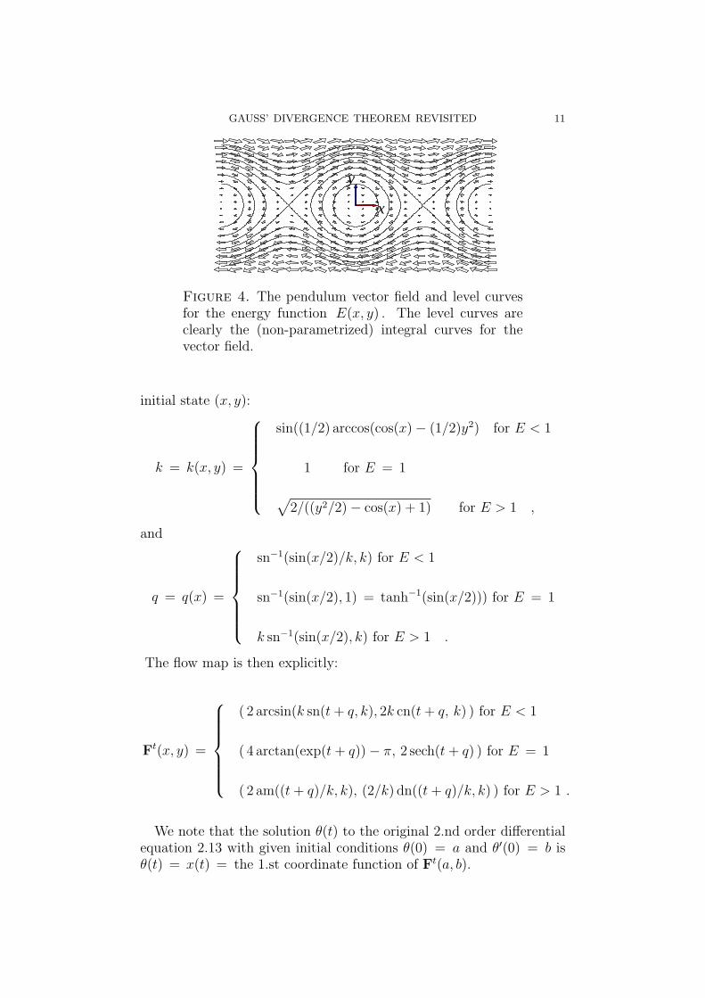
Here E = E(x, y) = (1/2)y2− cos(x) (once set into swing with thisinitial energy, the pendulum preserves this energy for all times): The’back and forth’ mode with small energy: E = (y2/2) − cos(x) < 1and the ’revolving’ mode with large energy: E = (y2/2)−cos(x) > 1 .In ’between’ these two modes, the ’separating’ mode is determined byE = (y2/2)− cos(x) = 1.
The constant energy is composed of potential and kinetic energy.The integral curves are (non-parametrized) level curves for this energyfunction, see Figure 4. The hard part of this example (as in general)is to actually parametrize these integral curves by time.
We let am, cn, sn, and dn denote Jacobi’s elliptic ’trigonometric’functions and denote by k and q the following values depending on the
GAUSS’ DIVERGENCE THEOREM REVISITED 11
y
x
Figure 4. The pendulum vector field and level curvesfor the energy function E(x, y) . The level curves areclearly the (non-parametrized) integral curves for thevector field.
initial state (x, y):
k = k(x, y) =
sin((1/2) arccos(cos(x)− (1/2)y2) for E < 1
1 for E = 1
√2/((y2/2)− cos(x) + 1) for E > 1 ,
and
q = q(x) =
sn−1(sin(x/2)/k, k) for E < 1
sn−1(sin(x/2), 1) = tanh−1(sin(x/2))) for E = 1
k sn−1(sin(x/2), k) for E > 1 .
The flow map is then explicitly:
Ft(x, y) =
( 2 arcsin(k sn(t + q, k), 2k cn(t + q, k) ) for E < 1
( 4 arctan(exp(t + q))− π, 2 sech(t + q) ) for E = 1
( 2 am((t + q)/k, k), (2/k) dn((t + q)/k, k) ) for E > 1 .
We note that the solution θ(t) to the original 2.nd order differentialequation 2.13 with given initial conditions θ(0) = a and θ′(0) = b isθ(t) = x(t) = the 1.st coordinate function of Ft(a, b).
12 S. MARKVORSEN
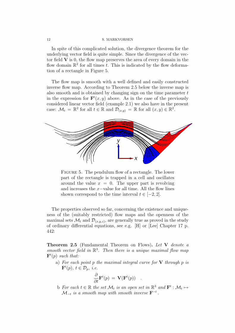
In spite of this complicated solution, the divergence theorem for theunderlying vector field is quite simple. Since the divergence of the vec-tor field V is 0, the flow map preserves the area of every domain in theflow domain R2 for all times t. This is indicated by the flow deforma-tion of a rectangle in Figure 5.
The flow map is smooth with a well defined and easily constructedinverse flow map. According to Theorem 2.5 below the inverse map isalso smooth and is obtained by changing sign on the time parameter tin the expression for Ft(x, y) above. As in the case of the previouslyconsidered linear vector field (example 2.1) we also have in the presentcase: Mt = R2 for all t ∈ R and D(x,y) = R for all (x, y) ∈ R2.
x
y
Figure 5. The pendulum flow of a rectangle. The lowerpart of the rectangle is trapped in a cell and oscillatesaround the value x = 0. The upper part is revolvingand increases the x−value for all time. All the flow linesshown correspond to the time interval t ∈ [−2, 2].
The properties observed so far, concerning the existence and unique-ness of the (suitably restricted) flow maps and the openness of themaximal sets Mt and D(x,y,z), are generally true as proved in the studyof ordinary differential equations, see e.g. [H] or [Lee] Chapter 17 p.442:
Theorem 2.5 (Fundamental Theorem on Flows). Let V denote asmooth vector field in R3. Then there is a unique maximal flow mapFt(p) such that:
a) For each point p the maximal integral curve for V through p isFt(p), t ∈ Dp, i.e.
∂
∂tFt(p) = V(Ft(p)) .
b For each t ∈ R the set Mt is an open set in R3 and Ft : Mt 7→M−t is a smooth map with smooth inverse F−t .
GAUSS’ DIVERGENCE THEOREM REVISITED 13
3. The curve flow and covariant derivatives
Note that at points where V(x, y, z) = (0, 0, 0) the flow map of thevector field V is the identity for all t. There is no flow, no deformationof such points or point sets. When V 6= (0, 0, 0), the flow map Ft
moves - and in general deforms - any given smooth curve, surface ordomain into a new smooth curve, surface and domain - see Figures 1and 2. The main idea in the present paper is to understand Gauss’divergence theorem in terms of this deformation. In fact we only needto understand the t−derivative of the deformation at t = 0 in orderto extract the divergence theorem from such an analysis.
We begin by studying in detail what happens to a given parametrizedcurve r(u), u ∈ [a, b], when it is floating along a given vector field V.The first obvious question concerns the length of the deformed curveFt(r(u)). To find the length we need to find the tangent vector fieldalong the curve, i.e. the vector field ∂
∂uFt(r(u)) for every u ∈ [a, b]. For
this purpose we need to introduce the so-called covariant derivative ofthe vector field.
Definition 3.1. Let V denote a smooth vector field with coordinatefunctions V(x, y, z) = (V1(x, y, z), V2(x, y, z), V3(x, y, z)) and let X =(X1, X2, X3) be any (other) smooth vector field in R3. The covariantderivative of V with respect to X is then the following vector field:
(3.1) ∇XV = [ DV] X ,
where [ DV] denotes the matrix (operator):
(3.2) [ DV] =
∂V1
∂x∂V1
∂y∂V1
∂z∂V2
∂x∂V2
∂y∂V2
∂z∂V3
∂x∂V3
∂y∂V3
∂z
.
When evaluating the right hand side of (3.1) we get
(3.3)∇XV =
(X1
∂V1
∂x+ X2
∂V1
∂y+ X3
∂V1
∂z, ∗ , ∗
)
= (grad(V1) ·X , grad(V2) ·X , grad(V3) ·X) ,
so that the covariant derivative is - in this precise sense - the directionalderivative of V with respect to X.
We note that the divergence of V is precisely the trace of the matrix[ DV]. This trace will appear below when we express the local volumedeformation (via the Jacobian) induced by the flow map on a givendomain.
The covariant derivative appears naturally from an application ofthe chain rule as follows: We evaluate the vector field V along a given
14 S. MARKVORSEN
parametrized curve r(u) and consider the u−derivative of the coordi-nate functions Vi(r(u)) , i = 1, 2, 3 , i.e.
(3.4)∂
∂uVi(r(u)) = grad(Vi) · r′(u) .
In view of equation (3.3) we therefore have:
Lemma 3.2.
(3.5)∂
∂uV(r(u) = [ DV]|r(u)
r′(u) .
We are now ready to set free the curve and let it flow along theintegral curves of the vector field.
Proposition 3.3. Given a smooth parametrized curve r(u), u ∈ [a, b].When the points of this curve flow along their respective integral curvesof V, the deformed curve Ft(r(u)) has the following tangent vector fieldat time t:
(3.6)∂
∂uFt(r(u)) =
(I + t
([ DV]|r(u)
+[D εt
]|r(u)
))r′(u) ,
where I denotes the identity matrix and [ D εt]|(t,x,y,z)is a matrix func-
tion all of whose elements go to 0 when t → 0.
Proof. By definition we know the t−derivative of Ft in terms of thevector field V, see Theorem 2.5:
(3.7)∂
∂tFt(x, y, z) = V(Ft(x, y, z)) .
The Taylor series expansion of Ft(x, y, z) with respect to t at t = 0 forfixed (x, y, z) is therefore:
(3.8)
Ft(x, y, z) = F0(x, y, z) + t
(∂
∂t
)
|t=0
Ft(x, y, z) + t εt(x, y, z)
= (x, y, z) + tV(F0(x, y, z)) + t εt(x, y, z)
= (x, y, z) + tV(x, y, z) + t εt(x, y, z) ,
where εt has the property that εt(x, y, z) → 0 for t → 0 and for all(x, y, z). Moreover it follows from equation (3.8) that for every fixedvalue of t in D(x,y,z) the function εt(x, y, z) is a smooth function of thethree space variables x, y, and z. In coordinates, let
εt(x, y, z) = (εt1(x, y, z), εt
2(x, y, z), εt3(x, y, z)) .
The covariant derivative matrix for εt (with respect to the space vari-ables) is then:
(3.9)[D εt
]|(x,y,z)
=
∂εt1
∂x
∂εt1
∂y
∂εt1
∂z∂εt
2
∂x
∂εt2
∂y
∂εt2
∂z∂εt
3
∂x
∂εt3
∂y
∂εt3
∂z
.
GAUSS’ DIVERGENCE THEOREM REVISITED 15
Since the derivatives entering this matrix are derivatives with respectto the space variables only, the matrix [ D εt] retains the property thatall the elements of [ D εt]|(t,x,y,z)
go to 0 for t → 0 .
Along the curve r(u) we then have directly from (3.8)
(3.10) Ft(r(u)) = r(u) + t(V(r(u)) + εt(r(u))
),
where εt(r(u)) is now a smooth function of u with:
(3.11)∂
∂uεt(r(u)) =
[D εt
]|r(u)
r′(u) .
In consequence, upon differentiation of equation (3.10) with respect tou, we arrive at the desired relation:
(3.12)
∂
∂uFt(r(u)) = r′(u) + t
([ DV]|r(u)
+[D εt
]|r(u)
)r′(u)
=(I + t
([ DV]|r(u)
+[D εt
]|r(u)
))r′(u) .
¤
Definition 3.4. The map of the tangent vector r′(u) to the correspond-ing tangent vector of the deformed curve found at the right hand sideof (3.12) is called the vectorial push forward map associated with thevector field V. This map only depends on time t and position p = r(u)and is given explicitly by (3.6). We denote it by:
(3.13) Ft∗|p = I + t
([ DV]|p +
[D εt
]|p
),
so that (3.12) now reads
(3.14)∂
∂uFt(r(u)) = Ft
∗|r(u)r′(u) = Ft
∗ r′(u) .
For fixed values of t and p the map Ft∗|p is a linear (matrix valued)
map or operator which maps (tangent) vectors at p to (tangent) vec-tors at Ft(p). The dependence of Ft
∗ on position - here r(u) - will often(as on the rightmost side of (3.14)) be suppressed from the notation,whenever there is no danger of confusion.
For later use (in section 5) we note here the following properties ofpush forward maps:
Lemma 3.5. If we apply the push forward map associated with a givenvector field V to the vector field itself we get
(3.15) Ft∗|p V(p) = V(Ft(p)) .
In other words, the vectorial push forward map associated with a givenvector field V preserves this vector field.
16 S. MARKVORSEN
Proof. Let γ(u) denote the maximal integral curve for V through thepoint p so that γ ′(u) = V(γ(u)) and γ(0) = p . By uniquenessof integral curves, Ft maps the integral curve γ(u) into itself. Thecorresponding vectorial push forward map Ft
∗ maps tangent vectors ofa curve to tangent vectors of the image curve. In particular, the tangentvector γ ′(0) at γ(0) is therefore mapped into the tangent vector γ ′(ut)at γ(ut), where ut is that parameter value which corresponds to thepoint Ft(γ(u0)), i.e. γ(ut) = Ft(γ(u0)). (Actually ut = u0 + t , butwe shall not need this fact.) Thus we have
(3.16) Ft∗ γ ′(u0) = γ ′(ut) ,
so that
(3.17)
Ft∗V(p) = V(γ(ut))
= V(Ft(γ(u0)))
= V(Ft(p)) .
¤
Proposition 3.6. The push forward map enjoys - and is in fact de-termined by - the following matrix differential equation along any givenintegral curve Ft(p), t ∈ Dp, for the vector field V:
(3.18)∂
∂tFt∗|p = [ DV]|Ft(p)
Ft∗|p , F0
∗|p = I .
Proof. Let t0 ∈ Dp be a fixed parameter value and assume s sufficientlysmall, so that t0 + s ∈ Dp. Then by construction
(3.19) Ft0+s∗|p = Fs
∗|Ft0 (p)
Ft0∗|p ,
where the right hand side is the matrix product of the two matricescorresponding to the two-step vectorial push forward - first from p toFt0(p) and then from Ft0(p) to Ft0+s(p) along the same integral curve.It follows that
(3.20)
(∂
∂t
)
|t=t0
Ft∗|p =
(∂
∂s
)
|s=0
Ft0+s∗|p
=
((∂
∂s
)
|s=0
Fs∗|
Ft0 (p)
)Ft0∗|p
= [ DV]|Ft0 (p)
Ft0∗|p .
The latter identity - as well as the initial condition in (3.18) - followsdirectly from (3.13). ¤
The following important identity relates the determinant and thetrace of time dependent linear maps (matrices) like Ft
∗(p) :
GAUSS’ DIVERGENCE THEOREM REVISITED 17
Theorem 3.7 (Liouville, see e.g. [H] p. 46). Let A(t) denote a givensquare matrix-valued smooth function of t. Let Y = Y(t) be a matrixsolution to the first order linear matrix differential equation:
(3.21)d
dtY(t) = A(t)Y(t) .
Then
(3.22) det(Y(t)) = det(Y(0)) exp
(∫ t
0
trace(A(s)) ds
),
so that
(3.23)d
dtdet(Y(t)) = trace(A(t)) det(Y(t)) .
In our case we thus have along every integral curve Ft(p) for V:
Corollary 3.8 (See [Ar] p. 112 for no less than two elementary proofs).
(3.24)
d
dtdet(Ft
∗|p) = trace([ DV]|Ft(p)) det(Ft
∗|p)
= div(V)|Ft(p)det(Ft
∗|p) ,
so that in particular, at t = 0, where det(F0∗|p) = det(I) = 1 we get:
(3.25)
(d
dt
)
|t=0
det(Ft∗|p) = trace([ DV]|p)
= div(V)(p) .
Example 3.9 (Example 2.3 continued). In order to illustrate the in-ner workings of these findings we show a few explicit calculationsconcerning the vector field in Example 2.3. So let r(u) denote asmooth curve and let Ft denote the flow map for the vector fieldV(x, y, z) = (−y, x, z2). Then we have from (2.7) that
Ft(r(u)) = Ft(x(u), y(u), z(u))
= ( x(u) cos(t)− y(u) sin(t),
x(u) sin(t) + y(u) cos(t),
z(u)/(1− tz(u)) ) .
In consequence
∂
∂uFt(r(u)) = ( x′(u) cos(t)− y′(u) sin(t),
x′(u) sin(t) + y′(u) cos(t),
z′(u)/(1− tz(u))2 )
=
cos(t) − sin(t) 0sin(t) cos(t) 0
0 0 1/(1− tz(u))2
x′(u)y′(u)z′(u)
18 S. MARKVORSEN
At the point (x, y, z) = p we thus get the vectorial push forward mapassociated with V:(3.26)
Ft∗|p =
cos(t) − sin(t) 0sin(t) cos(t) 0
0 0 1/(1− tz)2
=
1− t ε(t) −t + t ε(t) 0t− t ε(t) 1− t ε(t) 0
0 0 1 + 2t z + t ε(t, z)
=
1 0 00 1 00 0 1
+ t
0 −1 01 0 00 0 2 z
+ t
−ε(t) ε(t) 0−ε(t) −ε(t) 0
0 0 ε(t, z)
for suitable ε−functions. Since the covariant derivative of V in thisexample is given by
(3.27) [ DV]|(x,y,z)=
0 −1 01 0 00 0 2 z
,
we have thereby verified Proposition 3.3 in this particular case. More-over, using the exact expressions for Ft(p) from equation (2.7) and Ft
∗|pfrom equation (3.26) it is a direct matter to verify Proposition 3.6 andCorollary 3.8 as well. In particular we note that along the integralcurve starting at p = (x, y, z) the determinant of the push forwardmap is
(3.28) det(Ft∗|p) =
1
(1− t z)2.
This is in accordance with the fact, that t must belong to Dp : If, say,z > 0 or z < 0, then neither the flow nor the push forward map isdefined past the time value t = 1/z. On the other hand, if z = 0,then the flow and the push forward is defined for all values of t anddet(Ft
∗|p) = 1 for all t ∈ R. This is due to the fact, that all points in the
(x, y)−plane are just rotated in that plane by the flow map. A smoothcurve r(u), u ∈ [a, b], which crosses once through the (x, y)−planeis certainly deformed by the flow: as time goes by all the points ofthe curve - except the point of crossing - will race towards infinity.Nevertheless, the tangent vector to the curve at the cross point willkeep its length and will just rotate around the z−axis (with a fixed3.rd coordinate) along with the point of crossing.
4. The volume flow and the first half of the theorem
We now consider a 3D domain Ω0 in space and assume without lackof generality that Ω0 is represented by a piecewise smooth and regular
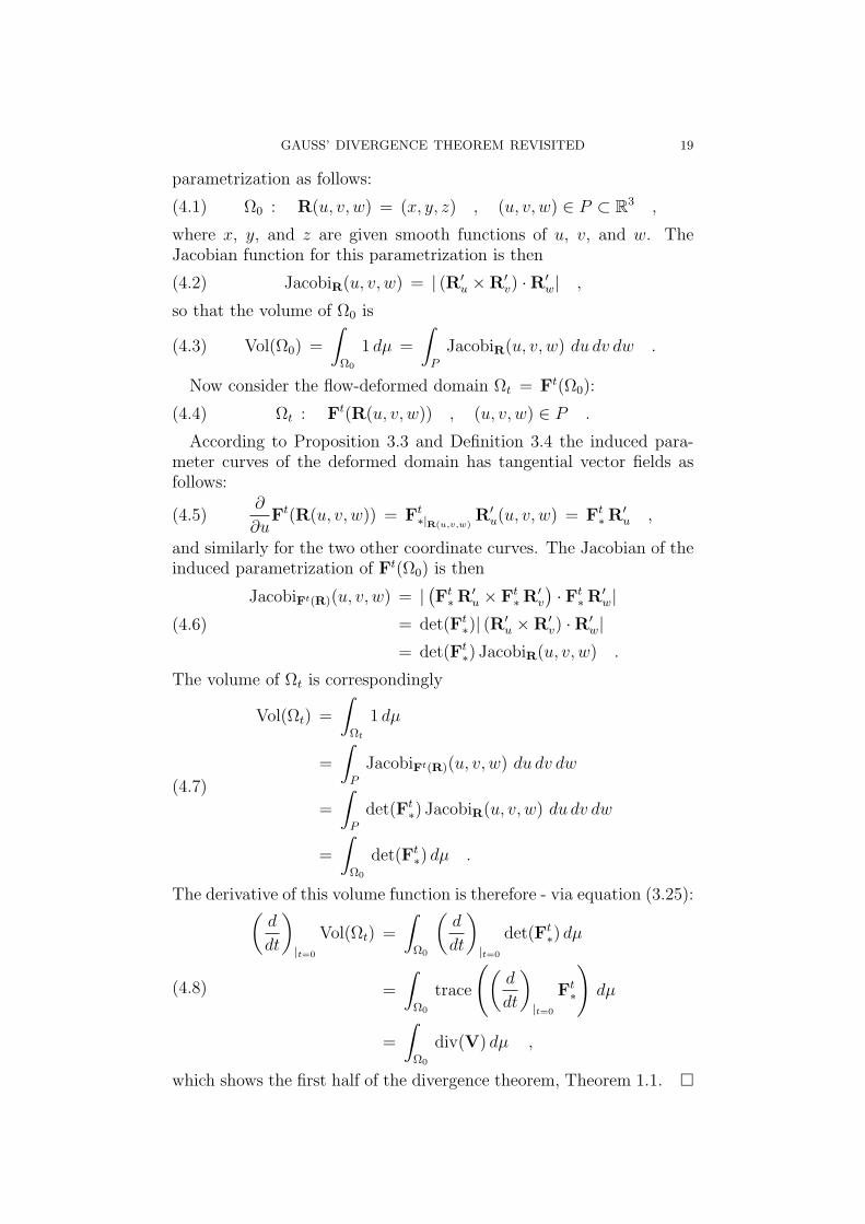
GAUSS’ DIVERGENCE THEOREM REVISITED 19
parametrization as follows:
(4.1) Ω0 : R(u, v, w) = (x, y, z) , (u, v, w) ∈ P ⊂ R3 ,
where x, y, and z are given smooth functions of u, v, and w. TheJacobian function for this parametrization is then
(4.2) JacobiR(u, v, w) = | (R′u ×R′
v) ·R′w| ,
so that the volume of Ω0 is
(4.3) Vol(Ω0) =
∫
Ω0
1 dµ =
∫
P
JacobiR(u, v, w) du dv dw .
Now consider the flow-deformed domain Ωt = Ft(Ω0):
(4.4) Ωt : Ft(R(u, v, w)) , (u, v, w) ∈ P .
According to Proposition 3.3 and Definition 3.4 the induced para-meter curves of the deformed domain has tangential vector fields asfollows:
(4.5)∂
∂uFt(R(u, v, w)) = Ft
∗|R(u,v,w)R′
u(u, v, w) = Ft∗R
′u ,
and similarly for the two other coordinate curves. The Jacobian of theinduced parametrization of Ft(Ω0) is then
(4.6)
JacobiFt(R)(u, v, w) = | (Ft∗R
′u × Ft
∗R′v
) · Ft∗R
′w|
= det(Ft∗)| (R′
u ×R′v) ·R′
w|= det(Ft
∗) JacobiR(u, v, w) .
The volume of Ωt is correspondingly
(4.7)
Vol(Ωt) =
∫
Ωt
1 dµ
=
∫
P
JacobiFt(R)(u, v, w) du dv dw
=
∫
P
det(Ft∗) JacobiR(u, v, w) du dv dw
=
∫
Ω0
det(Ft∗) dµ .
The derivative of this volume function is therefore - via equation (3.25):
(4.8)
(d
dt
)
|t=0
Vol(Ωt) =
∫
Ω0
(d
dt
)
|t=0
det(Ft∗) dµ
=
∫
Ω0
trace
((d
dt
)
|t=0
Ft∗
)dµ
=
∫
Ω0
div(V) dµ ,
which shows the first half of the divergence theorem, Theorem 1.1. ¤
20 S. MARKVORSEN
5. Surface flow and the second half of the theorem
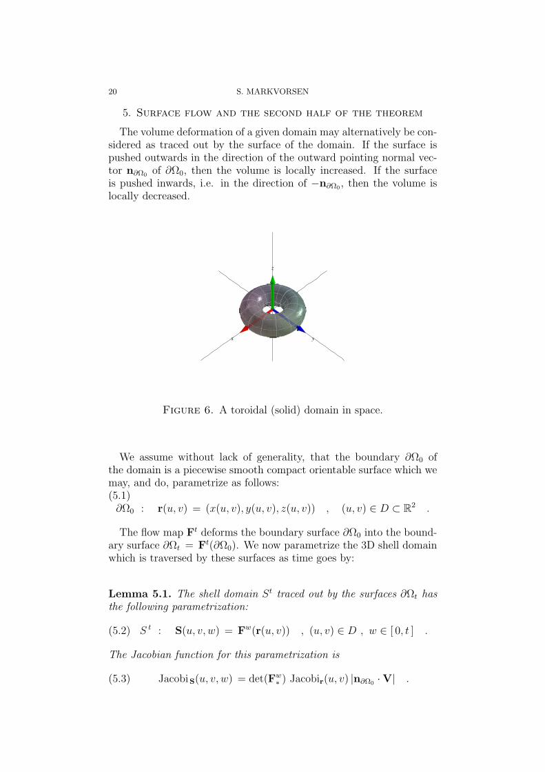
The volume deformation of a given domain may alternatively be con-sidered as traced out by the surface of the domain. If the surface ispushed outwards in the direction of the outward pointing normal vec-tor n∂Ω0 of ∂Ω0, then the volume is locally increased. If the surfaceis pushed inwards, i.e. in the direction of −n∂Ω0 , then the volume islocally decreased.
yx
z
Figure 6. A toroidal (solid) domain in space.
We assume without lack of generality, that the boundary ∂Ω0 ofthe domain is a piecewise smooth compact orientable surface which wemay, and do, parametrize as follows:(5.1)
∂Ω0 : r(u, v) = (x(u, v), y(u, v), z(u, v)) , (u, v) ∈ D ⊂ R2 .
The flow map Ft deforms the boundary surface ∂Ω0 into the bound-ary surface ∂Ωt = Ft(∂Ω0). We now parametrize the 3D shell domainwhich is traversed by these surfaces as time goes by:
Lemma 5.1. The shell domain St traced out by the surfaces ∂Ωt hasthe following parametrization:
(5.2) S t : S(u, v, w) = Fw(r(u, v)) , (u, v) ∈ D , w ∈ [ 0, t ] .
The Jacobian function for this parametrization is
(5.3) JacobiS(u, v, w) = det(Fw∗ ) Jacobir(u, v) |n∂Ω0 ·V| .
GAUSS’ DIVERGENCE THEOREM REVISITED 21
Proof. Using Proposition 3.3 and Lemma 3.5 we obtain the respectivederivatives:
(5.4)
S′u(u, v, w) =∂
∂uFw(r(u, v))
= Fw∗ r′u(u, v) ,
S′v(u, v, w) =∂
∂vFw(r(u, v))
= Fw∗ r′v(u, v) , and
S′w(u, v, w) =∂
∂wFw(r(u, v))
= V(Fw(r(u, v)))
= V(S(u, v, w))
= Fw∗ V(S(u, v, 0))
= Fw∗ V(r(u, v)) .
The Jacobian function of the shell parametrization is thence:
(5.5)
JacobiS(u, v, w) = |(S′u × S′v) · S′w|= | (Fw
∗ r′u × Fw∗ r′v) · Fw
∗ V|= det(Fw
∗ ) | (r′u × r′v) ·V| .
Since we also have by definition that
r′u × r′v = Jacobir(u, v)n∂Ω0 ,
we therefore get as claimed:
(5.6) JacobiS(u, v, w) = det(Fw∗ ) Jacobir(u, v) |n∂Ω0 ·V| .
¤
The final key point is now to observe, that the previously consideredvolume Vol(Ωt) is precisely the volume of Ω0 plus the signed volume ofthe shell S t, the sign being determined by n∂Ω0 ·V as alluded to above:
Vol(Ωt) = Vol(Ω0) +
∫
St
sign(n∂Ω0 ·V) dµ
= Vol(Ω0) +
∫ t
0
(∫
D
sign(n∂Ω0 ·V) JacobiS(u, v, w) du dv
)dw
= Vol(Ω0) +
∫ t
0
(∫
D
(n∂Ω0 ·V) det(Fw∗ ) Jacobir(u, v) du dv
)dw
= Vol(Ω0) +
∫ t
0
(∫
∂Ω0
det(Fw∗ ) (n∂Ω0 ·V) dν
)dw ,
22 S. MARKVORSEN
so that, using det(F0∗) = det(I) = 1 we finally get from an application
of the Fundamental Theorem of Calculus, Theorem 1.2:(
d
dt
)
|t=0
Vol(Ωt) =
(d
dt
)
|t=0
∫ t
0
(∫
∂Ω0
det(Fw∗ ) (n∂Ω0 ·V) dν
)dw
=
∫
∂Ω0
det(F0∗) (n∂Ω0 ·V) dν
=
∫
∂Ω0
n∂Ω0 ·V dν ,
which then proves ’the second half’ of Theorem 1.1.
¤
In closing we note that the proof presented here is easily lifted almostverbatim to vector fields and domains in Rn for n > 3.
For planar vector fields and planar domains, i.e. for n = 2, the di-vergence theorem follows directly from the 3D version presented above.Indeed, the vector field should just be extended to have 0 as a constantthird coordinate and the domain be extended to a finite height 3D cylin-drical domain with the given 2D domain as cross section. Then The-orem 1.1 gives the 2D statement except for a constant factor, namelythe height of the chosen cylinder.
For n = 1, the divergence theorem is, of course, nothing but theFundamental theorem of Calculus, Theorem 1.2.
References
[A] A. Altintas, Archimedes’ Principle as an Application of the DivergenceTheorem, IEEE Transactions on Education, Vol. 33, No. 2, May 1990,p. 222.
[Ar] V. I. Arnold, Ordinary Differential Equations (Translated and edited byR. A. Silverman), MIT Press (1973).
[C] M. J. Crowe, A History of Vector Analysis, University of Notre DamePress (1967).
[DoB] Y. J. Dori and J. Belcher, How does technology-enabled active learningaffect undergraduate student’s understanding of electromagnetism con-cepts?, Journal of the Learning Sciences 14 (2) 2005, 243-280.
[DuB] J. W. Dunn and J. Barbanel, One model for an integrated math/physcourse focusing on electricity and magnetism and related calculus topics,Am. J. Phys. 68 (8), August 2000, pp. 749–757.
[EP] C. H. Edwards and D. E. Penney, Calculus, Sixth Edition, Prentice Hall(2002).
[ES] B. Eisenberg and R. Sullivan, The Fundamental Theorem of Calculus inTwo Dimensions, Am. Math. Monthly 109, November 2002.
GAUSS’ DIVERGENCE THEOREM REVISITED 23
[FLS] R. P. Feynman, R. B. Leighton, and M. Sands, The Feynman Lectureson Physics, Vol. II, Addison Wesley (1965).
[Gre] G. Green, An Essay on the Application of Mathematical Analysis to theTheories of Electricity and Magnetism, Nottingham (1828).
[H] P. Hartman, Ordinary Differential Equations, Second Edition,Birkhauser (1982).
[Law] D. F. Lawden, Elliptic Functions and Applications, Springer-Verlag, NewYork (1989).
[Lee] J. M. Lee, Introduction to Smooth Manifolds, Springer (2003).[MacM] W. D. MacMillan, Statics and the Dynamics of a Particle, Dover (1958).[Mar] S. Markvorsen, The classical version of Stokes’ theorem revisited, Mat-
Report No. 2005-09, April 2005, 12 pages.[P] H. Pleym, Maple worksheets for Calculus, CD-ROM attachment to [EP],
Prentice Hall (2002).[She] J. A. Shercliff, Vector fields; Vector analysis developed through its ap-
plication to engineering and physics, Cambridge University Press, Cam-bridge (1977).
Department of Mathematics and Learning Lab DTU, Technical Uni-versity of Denmark, Building 303 and 101, DK-2800 Lyngby Denmark.
E-mail address: [email protected]


![Second Year (Information Technology) · PDF fileSecond Year (Information Technology) (With effect from A.Y 2009-10) ... 4.5 Gauss Divergence Theorem [without proof] and its applications](https://img.pdfslide.us/doc/110x75/5abd653f7f8b9ad8278bc15f/second-year-information-technology-year-information-technology-with-effect.jpg)