Embed Size (px)
Citation preview
The Dimensions of Consensus
Alex Gershkov, Benny Moldovanu and Xianwen Shi∗
October 26, 2017
Abstract
We study a multi-dimensional collective decision under incomplete informa-
tion. Agents have Euclidean preferences and vote by simple majority on each
issue (dimension), yielding the coordinate-wise median. Judicious rotations of
the orthogonal axes —the issues that are voted upon —lead to welfare improve-
ments. If the agents’ types are drawn from a distribution with independent
marginals then, under weak conditions, voting on the original issues is not op-
timal. If the marginals are identical (but not necessarily independent), then
voting first on the total sum and next on the differences is often welfare supe-
rior to voting on the original issues. We also provide various lower bounds on
incentive effi ciency: in particular, if agents’types are drawn from a log-concave
density with symmetric marginals, a second-best voting mechanism attains at
least 88% of the first-best effi ciency.
1 Introduction
In 1974 the U.S. Congress changed its budgeting process: instead of considering
appropriations requests that were voted upon one at a time (bottom-up) which resulted
in a gradually determined total level of spending, the Congressional Budget and
∗We wish to thank Yeon-Koo Che, Rahul Deb, Hans-Peter Grüner, Philippe Jehiel, Andreas
Kleiner, Robert J. McCann, Konrad Mierendorff, Marcin Peski, Rob Ready, Colin Stewart, Thomas
Tröger, Jürgen von Hagen and Cedric Wasser for helpful comments, and to various seminar and
conference participants for helpful discussions. Shuangjian Zhang provided excellent research assis-
tance. Shi is grateful to Social Sciences and Humanities Research Council of Canada for financial
support. Gershkov: Department of Economics, Hebrew University of Jerusalem, Israel and School
of Economics, University of Surrey, UK, [email protected]; Moldovanu: Department of Economics,
University of Bonn, Germany, [email protected]; Shi: Department of Economics, University of
Toronto, Canada, [email protected].
1

Impoundment Control Act required voting first on an overall level of spending, before
the determination of budgets for individual programs in subsequent votes (top-down).
A large literature in the area of public finance (see for example the review articles in
Poterba and von Hagen [1999]) has debated the costs and benefits of such proceduralchanges, with particular attention to the size of the expected budget deficit.1
In this paper we analyze the general problem of redefining (or bundling) the issues
brought to vote in a multi-dimensional collective decision problem. Our interest in
this topic stems from the potential of such methods to increase the welfare of the
involved decision makers by allowing them to reach, in an incentive compatible way,
a consensus that was not possible on the original issues. We are thus looking for
the dimensions on which the best consensus can be found, or, put differently, the
dimensions where the least cleavage among voters is present.
We study a multi-dimensional collective decision that is resolved via simple major-
ity voting: an example is a legislature that needs to decide on individual budgets for
public goods such as, say, education and defence. Another example is the decision on
the geographical location of a desirable facility. But even “mundane”decisions such
as hiring or project adoption based on multi-dimensional attributes can be viewed
through our lens.
We adopt the standard spatial model of voting widely used in the political science
literature (see for example, Chapter 5 in Austen-Smith and Banks [2005]), where
voters have preferences characterized by ideal points in each dimension and by a
quadratic loss caused by deviations from the ideal point. The main text deals with
the two-dimensional case, while the generalization to more than two dimensions is in
an Appendix.
The voters’ideal points are private information, and we look at the outcomes of
voting by simple majority on each dimension separately – as we shall see below, the
focus on simple majority voting yields, in combination with a decision over the dimen-
sions that are the subject of voting, an analysis of more generality than immediately
apparent.
With votes taken by simple majority in each separate dimension, the outcome
is the coordinate-wise median of the voters’ ideal points. This easily follows from
Black’s [1948] famous theorem because the induced preferences are single peaked
on each one-dimensional issue. In general, this outcome does not coincide with the
first-best, given here by the alternative that minimizes the overall distance from the
individual ideal points. It is of course well-known that the first-best outcome is simply
1There was a widespread belief that the new rules would lead to smaller deficits, and the act was
passed almost unanimously in both House and Senate.
2
the coordinate-wise average (or mean) of the ideal points, and thus first-best welfare
is given here by the corresponding variance (with a minus sign).
The first-best outcome is not implementable: each agent has an incentive to try
to move the average closer to his/her ideal point by exaggerating his/her position
on one or more issues. This observation was first made by Galton [1907], who was
also the first to recommend the use of the median as a robust and non-manipulable
aggregator of opinions.2
Given the tension between first-best on the one hand and implementable outcomes
on the other, how well does voting by simple majority perform in terms of welfare?
Using a classical inequality due to Hotelling and Solomons [1932], it can be shown
that, for any distribution of preferences, voting by simple majority on any given issues
achieves at least 50% of the welfare achievable in the first best.
The main insight of the present paper is that a judicious choice of the issues
that are actually put to vote (while maintaining voting by simple majority, with
its desirable incentive properties) can significantly improve welfare.3 For example,
instead of voting on two separate issues such as education and health, the legislature
could vote on a total budget, and then on a division of that budget between the
two issues —just as Congress started to do in 1974. More generally, we model the
repackaging and bundling of issues by rotations of the orthogonal axes that define
what is put to vote. For example, suppose voters care about two separate main issues,
but they actually vote on the budget of two agencies that overlap in their responsibility
over these two issues. Rotations correspond then to the often observed shifting of
jurisdictions among the two agencies: they change the mix of issues under the control
of each agency. In an influential work, Shepsle [1979] argues that the division of a
complex, collective decision into several different jurisdictions (germaneness), creates
stable equilibria that would not be possible in a general, unconstrained collective
decision model. His main examples are the various legislative committees in the U.S.
congress. Viewed in light of Shepsle’s theory, our goal is to endogenize the choice of
jurisdictions in order to improve welfare, an issue that has not received much attention
in formal studies.
Our main results are:
1) If the agents’ideal points in one dimension are independently distributed from
the ideal points in the other dimension then, under weak conditions on the distribution
of preferences, voting on the original issues is sub-optimal; that is, a re-packaging of
the issues brought to vote via rotation (this necessarily creates some correlation among
2His insights have been sharpened and much generalized in the literature on robust estimation.3The idea of comparing voting rules in terms of their expected welfare goes back to Rae[1969].
3
the ideal points) increases welfare.
2) If the marginals of the distribution of agents’ideal points are identically distrib-
uted (but not necessarily independent), we provide suffi cient conditions under which
the 45-degree rotation is welfare superior to no rotation. The suffi cient conditions
are satisfied by commonly used distributions if marginals are identically and inde-
pendently distributed (I.I.D.). We show analytically that, with I.I.D. marginals, the
45-degree rotation is always a critical point, and numerically that it is a global wel-
fare maximum for many standard distributions. A key observation for these results
is that, under the symmetry of the marginals, the 45-degree rotation entirely elimi-
nates the conflict arising between effi ciency and majority voting in one dimension —
all remaining conflict is concentrated in the other, orthogonal dimension.
3)We provide various lower bounds on incentive effi ciency for large, non-parametric
families of distribution of ideal points (such as unimodal distributions, distributions
with an increasing hazard rate, etc.). For example, if agents’ideal points are drawn
from a log-concave density with I.I.D. marginals, a voting mechanism that involves
a 45 degrees rotation of the original dimensions attains at least 88% of the first-best
effi ciency. This should be compared to the universal lower bound of 50% that obtains
without any assumption on the distribution, and without using rotations.
We would like to point out here that some of our results are similar to the classical
insights, obtained in models with monetary transfers, about the benefits of bundling.
For example, the non-optimality of voting on independent issues parallels the non-
optimality of separate sales if the valuations on different objects are independent:
some form of mixed bundling is always superior (see McAfee, McMillan and Whinston
[1989]).4
The basic feature behind the welfare-improving properties of rotations is the non-
linearity of the median function, i.e. the median of a sum of random variables is
not equal to the sum of the medians. Note that the distributions of ideal points
after rotation can be represented as convolutions of the original distributions, which
explains here the appearance of sums of random variables. On the one hand, this
non-linearity is the driving force behind our results; on the other hand, it also implies
that the analysis becomes relatively complex.5 In order to use calculus and proba-
4In a similar vein, the need to control for sub/super-additivity of medians (see Section 3) parallels
the case of second-highest order statistics in auctions (see Palfrey [1983]), and the asymptotic effi -
ciency of the top-down budgeting procedure when the number of issues goes to infinity (see Section
4 below) corresponds to the asymptotic effi ciency of pure bundling when the number of objects goes
to infinity and marginal costs of production are zero (see Bakos and Brynjolfsson [1999]).
5This is true even for common distributions, such as the Gamma, Poisson, lognormal, etc. Some
4
bilistic/statistical techniques, we focus on the limit case where the number of voters
is infinite. In particular, we need to deal with order statistics of convolutions, and we
use various concentration inequalities that relate statistics such as the mean, median,
mode and variance of distributions.
1.1 Related Literature
It is well-known that the existence of a Condorcet winner is rare in multi-dimensional
models of voting (Kramer [1973]). Kramer [1972] observed that, however, voting in
a variety of institutions is often sequential, issue by issue, and he established that
there exists an issue-by-issue sophisticated voting equilibrium if voters’preferences
are continuous, convex and separable. The coordinate-wise median analyzed in our
paper —obtained by simple-majority voting in each dimension —constitutes a basic
instance of a structure induced equilibrium in the spirit of Shepsle [1979].
It is of course possible to perform an analysis similar to ours for goals other
than effi ciency, e.g., define jurisdictions that serve other purposes, such as the self-
interest of an agenda setter or of a coalition of voters. For example, Ferejohn and
Krehbiel [1987] observed that the 1974 budget reform can be represented by a 45-
degree rotation of the coordinates on which voting takes place. Their focus was on
controlling budgetary growth rather than effi ciency. Besides giving precise conditions
comparing the top-down and bottom-up procedures in terms of the total budget they
produce, we also show that the budgeting reform can unambiguously improve welfare
while having a mixed impact on the budget size!
Technically, our contribution builds upon and relates to several important and ele-
gant contributions due to Moulin [1980], Border and Jordan [1983], Kim and Rousch
[1984], and Peters, van der Stel and Storcken [1992]. In a one-dimensional setting
with single-peaked preferences, Moulin considered mechanisms that depend on re-
ported peaks, and characterized the set of dominant strategy incentive compatible
(DIC), anonymous and Pareto effi cient mechanisms: each mechanism in the class is
obtained by choosing the median among the n reported peaks of the real voters and
the peaks of a set of n − 1 “phantom” voters (these are fixed by the mechanism,
and do not vary with the reports).6 Border and Jordan [1983] removed Moulin’s
assumption whereby mechanisms were allowed to only depend on peaks, and gener-
alized Moulin’s finding to a multi-dimensional setting with separable and quadratic
preferences: each DIC mechanism was shown to be decomposable into a collection
of one-dimensional DIC mechanisms, each described by the location of the phantom
of our results are based on insights that go back to conjectures by Ramanujan (see Szegö [1928]).6Relaxing Pareto effi ciency yields the same characterization, but with n+ 1 phantoms.
5
voters in the respective dimension (see also Barbera, Gul and Stacchetti [1993]).7
Gershkov, Moldovanu and Shi [2016] analyzed welfare maximization in a one-
dimensional setting with cardinal utilities, and derived the ex-ante welfare maximiz-
ing placement of phantoms as a function of utilities and of the distribution of types.
They also showed how to avoid the phantom interpretation by implementing Moulin’s
mechanisms (including the welfare optimal one) via a sequential, binary voting pro-
cedure together with a flexible qualified majority schedule needed for the adoption of
various alternatives.8 Combining their result with the Border-Jordan decomposition
yields the welfare maximizing mechanism for multidimensional settings with separa-
ble and quadratic preferences. But, the ensuing solution, described by an optimal
placement of phantoms in each dimension, is not satisfactory from a practical point
of view: it implies that each issue (dimension) in each multi-dimensional problem
must be voted upon according to a particular institution. This theoretically needed
flexibility may be diffi cult, if not impossible, to achieve in practice.
Instead, we take here a different approach to welfare improvement: we fix an ubiq-
uitous institution —voting by simple majority on each issue —but we allow flexibility
in the design of the issues that are actually put to vote. Such a limited form of
agenda design is very common in practice, and, as we shall see, has important welfare
consequences.
The simplest multi-dimensional setting for studying issue design and repackaging is
the one with Euclidean preferences: intuitively, the presence of spherically symmetric
preferences does not a-priori determine the dimensions of the Border and Jordan
decomposition into one-dimensional mechanisms. Indeed, Kim and Rousch [1984]
showed that the set of continuous, anonymous and DIC mechanisms can be described
by performing the Border-Jordan analysis subsequent to any translation of the origin
and any rotation of the orthogonal axes. Peters, van der Stel and Storcken [1992]
showed that, for two dimensions, voting by simple majority in each dimension (after
any translation/rotation of the plane) is also Pareto optimal. This is the unique
anonymous and DIC mechanism with this property, and Pareto effi ciency is generally
not consistent with DIC in more than two dimensions.
Since both median and mean are translation equivariant, translations of the ori-
gin cannot improve welfare, and it is therefore without loss of generality to restrict
7Most papers in the literature indeed assume separable preferences. Ahn and Oliveros [2012] is a
notable exception: they prove equilibrium existence in combinatorial voting with non-separable pref-
erences, and provide conditions under which the Condorcet winner is implemented in the equilibrium
of large elections.8See also Kleiner and Moldovanu [2016] for a derivation of suffi cient conditions under which
sequential, binary voting procedures possess desirable properties.
6
attention to rotations of the axes followed by simple majority voting on each newly
defined dimension.
A key observation, well known in the theory of spatial statistics, is that the mean is
rotation equivariant (i.e., the mean after rotation is obtained by rotating the original
mean) but the coordinate-wise median is not (see Haldane [1948], or the literature on
spatial voting, e.g., Feld and Grofman [1988]). As a consequence, a rotation of the
axes may decrease the distance between the coordinate-wise mean (first-best) and the
coordinate-wise median (outcome of majority voting), thus increasing welfare in our
framework.
It is also instructive to compare our results to those in the classical papers by
Caplin and Nalebuff ([1988], [1991]) who did not consider incomplete information and
incentive constraints.9 Motivated by the instability of multi-dimensional voting, they
considered instead the effect of super-majority requirements on the stability of the
spatial mean. For a large number of voters and for log-concave density governing the
distribution of types (and also for other, more general forms of concavity). Caplin and
Nalebuff showed that, once established as status-quo, the mean cannot be displaced
by another alternative if the selection of that alternative requires a super-majority
of at least 64% (or 1− 1e). In other words, given the distributional assumptions and
a large population of voters, any coalition that prefers an alternative over the mean
contains less than 64% of the voters, and is thus not effective given the super-majority
requirement.
As mentioned above, for the log-concave case with independent marginals, our
results display a mechanism that is incentive compatible for any number of voters
and that achieves at least 88% of the first-best utility when this number goes to
infinity. Thus, issue by issue voting by simple majority on appropriately defined di-
mensions constitutes an intuitive and incentive compatible institutional arrangement
that is almost effi cient in this case. Moreover, the relative effi ciency of this mecha-
nism increases, and tends to 100% when we increase the number of dimensions of the
underlying problem.
Finally, although our model bears some similarity to models of multidimensional
cheap talk (see for example, Battaglini [2002], Chakraborty and Harbaugh [2007]),
the logic of welfare gains is very different here. In those models, the multiplicity of
issues helps because it improves information transmission between the sender and
the receiver(s). For example, in a model with two senders, Battaglini [2002] shows
that, as long as the two senders’ideal points are linearly independent (i.e., one is not
9These authors were also the first to use modern concentration inequalities in the Economics
literature.
7
a scalar multiple of the other), then full revelation is possible by carefully choosing
dimensions to exploit the conflict between senders. In a similar model with one
sender, Chakraborty and Harbaugh [2007] show that the sender can credibly convey
his ranking of different issues to the receiver. In contrast, in our model, private
information is fully revealed, because the information aggregation procedure, i.e.,
simple majority rule, is strategy-proof. Yet this rule does not lead to the effi cient
decision. Rotations deal here with a very different conflict, between the outcome
under simple majority and effi ciency. For example, in symmetric settings, the 45-
degree rotation improves welfare because it allows the designer to completely eliminate
this conflict in one dimension.
The remaining part of the paper is organized as follows: In Section 2 we present the
two dimensional voting model by simple majority, and connect incentive compatible
mechanisms to the special orthogonal group of rotations in the plane. We also discuss
the equi-invariance properties of means and medians. In Section 3 we focus on the
setting with a large number of agents, for which we can use various available statistical
techniques. We first show that voting on independent issues is always sub-optimal:
a rotation that bundles independent issues is always beneficial. We next show that
if the issues are identically distributed, a rotation by 45 degrees (corresponding, for
example, to a vote on a total budget for the two issues and its division among issues)
can improve welfare over the zero rotation. In particular, we give suffi cient conditions
that hold for large, non-parametric families of distributions under which the welfare
under such a rotation is higher than in the original, no-rotation case. Numerical
simulations suggest that the 45 degrees rotation is indeed an optimum in this case.
In Section 4 we offer bounds on the relative effi ciency of voting by simple majority
complemented by rotations. The effect of rotations is shown to be substantial. Section
5 concludes. Several proofs are gathered in Appendix A, and generalizations to higher
dimensions are sketched in Appendix B.
2 The Model
We consider an odd number of agents, n, who collectively decide about two issues,
X and Y , on a convex region D ⊆ R2. Each agent’s ideal position on these twoissues is given by a peak ti = (xi, yi), i = 1, 2, ..., n. The peak ti is agent i’s private
information. Each agent i has a utility function of the form
− ||ti − v||2
8
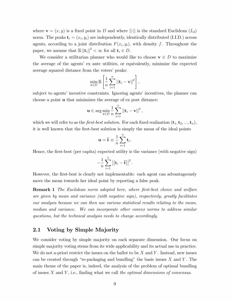
where v = (x, y) is a fixed point in D and where ||·|| is the standard Euclidean (L2)norm. The peaks ti = (xi, yi) are independently, identically distributed (I.I.D.) across
agents, according to a joint distribution F (xi, yi), with density f . Throughout the
paper, we assume that E ||ti||2 <∞ for all ti ∈ D.We consider a utilitarian planner who would like to choose v ∈ D to maximize
the average of the agents’ex ante utilities, or equivalently, minimize the expected
average squared distance from the voters’peaks:
minv∈D
E
[1
n
n∑i=1
||ti − v||2],
subject to agents’incentive constraints. Ignoring agents’incentives, the planner can
choose a point u that minimizes the average of ex post distance:
u ∈ arg minv∈D
1
n
n∑i=1
||ti − v||2 ,
which we will refer to as the first-best solution. For each fixed realization (t1, t2, ..., tn),
it is well known that the first-best solution is simply the mean of the ideal points
u = t ≡ 1
n
n∑i=1
ti.
Hence, the first-best (per capita) expected utility is the variance (with negative sign)
− 1
n
n∑i=1
∣∣∣∣ti − t∣∣∣∣2 .However, the first-best is clearly not implementable: each agent can advantageously
move the mean towards her ideal point by reporting a false peak.
Remark 1 The Euclidean norm adopted here, where first-best choice and welfare
are given by mean and variance (with negative sign), respectively, greatly facilitates
our analysis because we can then use various statistical results relating to the mean,
median and variance. We can incorporate other convex norms to address similar
questions, but the technical analysis needs to change accordingly.
2.1 Voting by Simple Majority
We consider voting by simple majority on each separate dimension. Our focus on
simple majority voting stems from its wide applicability and its actual use in practice.
We do not a-priori restrict the issues on the ballot to be X and Y . Instead, new issues
can be created through “re-packaging and bundling”the basic issues X and Y . The
main theme of the paper is, indeed, the analysis of the problem of optimal bundling
of issues X and Y , i.e., finding what we call the optimal dimensions of consensus.
9
2.2 Rotations in the Plane
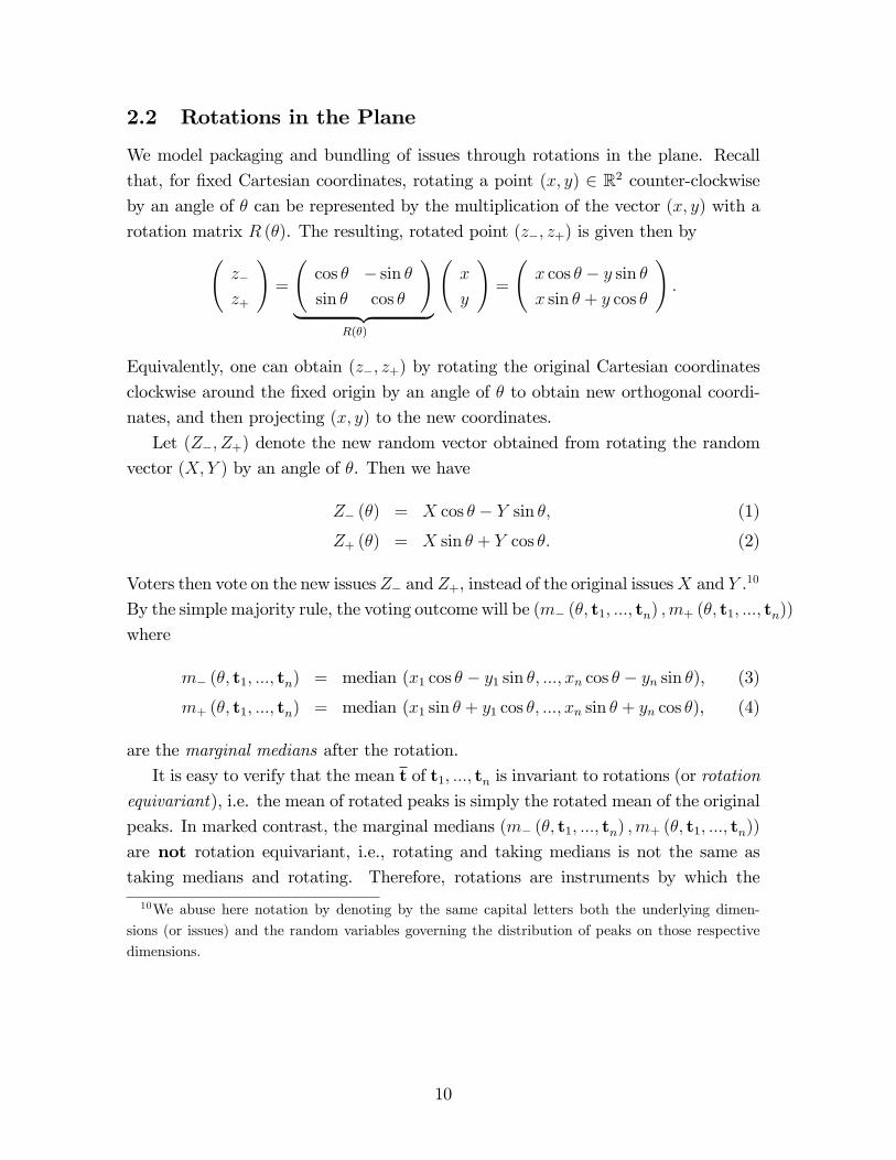
We model packaging and bundling of issues through rotations in the plane. Recall
that, for fixed Cartesian coordinates, rotating a point (x, y) ∈ R2 counter-clockwiseby an angle of θ can be represented by the multiplication of the vector (x, y) with a
rotation matrix R (θ). The resulting, rotated point (z−, z+) is given then by(z−
z+
)=
(cos θ − sin θ
sin θ cos θ
)︸ ︷︷ ︸
R(θ)
(x
y
)=
(x cos θ − y sin θ
x sin θ + y cos θ
).
Equivalently, one can obtain (z−, z+) by rotating the original Cartesian coordinates
clockwise around the fixed origin by an angle of θ to obtain new orthogonal coordi-
nates, and then projecting (x, y) to the new coordinates.
Let (Z−, Z+) denote the new random vector obtained from rotating the random
vector (X, Y ) by an angle of θ. Then we have
Z− (θ) = X cos θ − Y sin θ, (1)
Z+ (θ) = X sin θ + Y cos θ. (2)
Voters then vote on the new issues Z− and Z+, instead of the original issuesX and Y .10
By the simple majority rule, the voting outcome will be (m− (θ, t1, ..., tn) ,m+ (θ, t1, ..., tn))
where
m− (θ, t1, ..., tn) = median (x1 cos θ − y1 sin θ, ..., xn cos θ − yn sin θ), (3)
m+ (θ, t1, ..., tn) = median (x1 sin θ + y1 cos θ, ..., xn sin θ + yn cos θ), (4)
are the marginal medians after the rotation.
It is easy to verify that the mean t of t1, ..., tn is invariant to rotations (or rotation
equivariant), i.e. the mean of rotated peaks is simply the rotated mean of the original
peaks. In marked contrast, the marginal medians (m− (θ, t1, ..., tn) ,m+ (θ, t1, ..., tn))
are not rotation equivariant, i.e., rotating and taking medians is not the same astaking medians and rotating. Therefore, rotations are instruments by which the
10We abuse here notation by denoting by the same capital letters both the underlying dimen-
sions (or issues) and the random variables governing the distribution of peaks on those respective
dimensions.
10
planner may try to influence welfare.
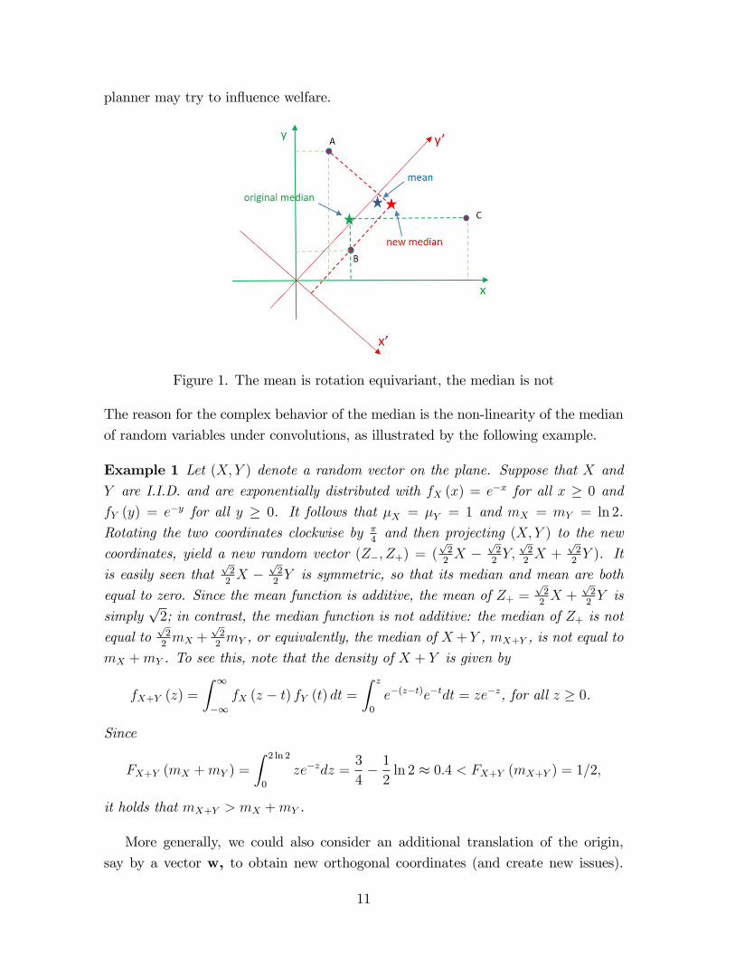
Figure 1. The mean is rotation equivariant, the median is not
The reason for the complex behavior of the median is the non-linearity of the median
of random variables under convolutions, as illustrated by the following example.
Example 1 Let (X, Y ) denote a random vector on the plane. Suppose that X and
Y are I.I.D. and are exponentially distributed with fX (x) = e−x for all x ≥ 0 and
fY (y) = e−y for all y ≥ 0. It follows that µX = µY = 1 and mX = mY = ln 2.
Rotating the two coordinates clockwise by π4and then projecting (X, Y ) to the new
coordinates, yield a new random vector (Z−, Z+) = (√22X −
√22Y,√22X +
√22Y ). It
is easily seen that√22X −
√22Y is symmetric, so that its median and mean are both
equal to zero. Since the mean function is additive, the mean of Z+ =√22X +
√22Y is
simply√
2; in contrast, the median function is not additive: the median of Z+ is not
equal to√22mX +
√22mY , or equivalently, the median of X +Y , mX+Y , is not equal to
mX +mY . To see this, note that the density of X + Y is given by
fX+Y (z) =
∫ ∞−∞
fX (z − t) fY (t) dt =
∫ z
0
e−(z−t)e−tdt = ze−z, for all z ≥ 0.
Since
FX+Y (mX +mY ) =
∫ 2 ln 2
0
ze−zdz =3
4− 1
2ln 2 ≈ 0.4 < FX+Y (mX+Y ) = 1/2,
it holds that mX+Y > mX +mY .
More generally, we could also consider an additional translation of the origin,
say by a vector w, to obtain new orthogonal coordinates (and create new issues).
11
The joint operation of rotation and translation can also be represented by a linear
matrix.11 But, medians (and means) are translation equivariant, and thus there is
no extra welfare advantage from such translations. Therefore, we focus below on the
family of rotations of coordinates around a fixed origin, described by the angle of
rotation θ relative to standard Cartesian coordinates.
2.3 The Set of Voting Mechanisms
For any rotation angle θ ∈ [0, 2π], we can define the direct marginal median mecha-
nism ϕθ as
ϕθ (t1, t2, ..., tn) = (m− (θ, t1, .., tn) ,m+ (θ, t1, .., tn)) ,
where (m− (θ, t1, .., tn) ,m+ (θ, t1, .., tn)) is the marginal median with respect to ro-
tation θ and reported peaks ti as defined in (3) and (4). Note that the function
ϕθ (t1, t2, ..., tn) is continuous in θ and in all its other arguments since both rotations
and medians are continuous functions. It is easy to see that ψθ is dominant-strategy
incentive compatible (DIC). Surprisingly, as shown by Kim and Roush [1984] and Pe-
ters et al. [1992], the set of marginal median mechanisms (for all possible rotations)
coincides with the entire class of anonymous, Pareto optimal and DIC mechanisms.12
This provides a complementary justification for our focus on simple-majority voting
mechanisms.
The mechanism ϕθ can be decentralized by defining the issues (via rotations) and
then voting sequentially by simply majority, one issue at a time, using a binary, se-
quential voting procedure with a convex agenda.13 To illustrate, suppose the two basic
issues X and Y are the levels of two public goods. For each (possibly rotated) dimen-
sion we separately apply the following sequential voting procedure, first devised by
11This set of general transformation matrices (rotation and translation) is called the special or-
thogonal group for the plane, and is denoted by SO(2). Each matrix in SO (2) is an orthogonal
matrix. It is special because the determinant of each matrix is +1, whereas the determinant could
be −1 for other orthogonal transformations such as reflections.12A mechanism ψ is anonymous if, for any profile of reports (ti, t−i), ψ (t1, ..., ti, ..., tn) =
ψ(tp(1), ..., tp(i), ..., tp(n)
), where p is any permutation of the set {1, ..., n}. A mechanism ψ is
Pareto optimal (or Pareto effi cient) if, for any profile of reports (ti, t−i), there is no alternative v
such that ||ti − v||2 ≤ ||ti − ψ (ti, t−i)||2 for all i, with strict inequality for at least one agent. Notethat their characterization fails in higher dimensions because anonymous, Pareto optimal and DIC
mechanisms need not exist. Hence, our analysis can be extended to higher dimensional problems,
but the solution need not be ex-post Pareto optimal.13At each stage of convex, sequential procedure on a fixed dimension, a binary decision is collec-
tively taken among two ideologically coherent sets of alternatives that create a clear left-right divide.
For details see Gershkov, Moldovanu and Shi (2016) and Kleiner and Moldovanu (2016).
12
Bowen [1943]: Starting with the status-quo quantity, voters vote by simple majority
on successive increments (or decrements); if a simple majority of voters is against the
first increment, voting stops and the status quo is adopted; otherwise voting contin-
ues to the next increment; if the second increment fails to garner a majority support,
voting stops and the first increment is implemented; otherwise, voting continues to
yet another increment, and so on. As argued in Bowen [1943], the sequential voting
procedure (where voters vote sincerely) yields an equilibrium level of public good pro-
vision that is preferred by the median voter of that dimension. Gershkov, Moldovanu
and Shi [2016] analyzed the dynamic, strategic incentives under Bowen’s procedure
and showed that sincere voting is also an ex-post equilibrium, and hence that the
public good level preferred by the median is indeed the equilibrium outcome. The
overall resulting equilibrium of sequential voting, dimension by dimension, is then an
incidence of the structure induced equilibrium à là Shepsle [1979].
Theorem 1 Assume that agents decide one issue at a time on the orthogonal dimen-sions Z+(θ) and Z−(θ) that are obtained by rotating original issues X and Y . Assume
also that the vote on each issue is by simple majority according to a convex, binary
sequential procedure. Then sincere voting is an ex-post equilibrium and the outcome
is (m− (θ, t1, ..., tn) ,m+ (θ, t1, ..., tn)), independently of the order in which the issues
are put up to vote.14
Proof. Assume that voters decide first on dimension Z+(θ), and then on dimension
Z−(θ), and recall that these are orthogonal. Denote the first decision by k+ (θ, t1, ..., tn).
This fixes the first coordinate of the final decision. In other words, at the second
stage the agents choose only among alternatives of the form (k+ (θ, t1, ..., tn) , z−).
This is a one-dimensional problem, on which agents have single peaked preferences.
For any k+ (θ, t1, ..., tn), the ex-post equilibrium outcome of any binary, sequential
voting with a convex agenda is sincere voting, and the outcome is the Condorcet
winner z− = m− (θ, t1, ..., tn). Given this outcome, the first decision is a choice
among alternatives of the form (z+,m− (θ, t1, ..., tn)). Since this is again a one-
dimensional problem, the outcome is the Condorcet winner, and the final outcome is
((m+ (θ, t1, ..., tn) ,m− (θ, t1, ..., tn)). An analogous reasoning yields the result for the
other order of votes on the two issues.14Sincere voting means that, at each binary decision node, an agent votes for the subset of alter-
natives containing his/her preferred alternative among those that are still relevant.
13
3 The Limit Case when the Number of Agents Is
Large
The full probabilistic optimization problem can be rewritten as
(P0) minθ∈[0,2π]
∫D
...
∫D
(1
n
n∑i=1
||R (θ) ti − ϕθ (t1, t2, ..., tn)||2)f(t1)...f(tn)dt1...dtn.
We focus here on the solution to problem (P0) when the number of agents is large.But, note that the resulting optimal mechanism will be incentive compatible, Pareto
optimal and anonymous for any number of voters.15 For a random variable X with
finite mean µX and variance σ2X , we know from the central limit theorem that
√n
(1
n
n∑i=1
Xi − µX
)→ N(0, σ2X).
Bahadur (1966) showed that the quantiles of large samples display a similar behavior.
In particular,√n(X(n+1)/2:n −mX)→ N
(0,
1
4f 2(mX)
)where
X(n+1)/2:n = median (X1, ..., Xn)
and where mX is the median of the distribution. Thus, as n goes to infinity, the
sample median converges to the median of the underlying distribution and, of course,
the sample mean converges to the mean.
By applying the above limit results to our setting, we obtain that, as n→∞,(m− (θ, t1, .., tn)
m+ (θ, t1, .., tn)
)−→
(m− (θ)
m+ (θ)
)≡(median (X cos θ − Y sin θ)
median (X sin θ + Y cos θ)
)Furthermore, since the norm operation ||·|| is continuous, we obtain that, as n→∞,
1
n
n∑i=1
||R (θ) ti − ϕθ (t1, t2, ..., tn)||2
=1
n
n∑i=1
[(xi cos θ − yi sin θ −m− (θ, t1, .., tn))2 + (xi sin θ + yi cos θ −m+ (θ, t1, .., tn))2
]→ E ||X cos θ − Y sin θ −m−(θ), X sin θ + Y cos θ −m+(θ)||2
= σ2X + σ2Y +(µ− (θ)−m− (θ)
)2+(µ+ (θ)−m+ (θ)
)215This contrasts trivial incentive compatible mechanisms such as always choosing a fixed alterna-
tive, which may yield “catastrophic”results for a finite number of agents and particular realizations
of types.
14
where
µ− (θ) = µX cos θ − µY sin θ, and µ+ (θ) = µX sin θ + µY cos θ
Therefore, in the limit where n is very large, our problem becomes
(P1) minθ∈[0,2π]
(µ− (θ)−m− (θ)
)2+(µ+ (θ)−m+ (θ)
)2+ σ2X + σ2Y .
In other words, we look for the rotation that creates the marginal median vector with
the minimum distance from the mean.
For most parts of the analysis below, it will be convenient to normalize the means
ofX and Y to be zero - such a normalization is without loss of generality because of the
translational equ-invariance of both mean and median. Let us define the normalized
random variables X and Y as
X = X − µX and Y = Y − µY .
The corresponding normalized marginal medians (m− (θ) , m+ (θ)) are
m− (θ) = m− (θ)− µ− (θ) and m+ (θ) = m+ (θ)− µ+ (θ) .
We further note that it is without loss of generality to restrict attention to rotations
in the interval [0, π/2]. That is, for any θ ∈ [π/2, 2π] that minimizes the planner’s
objective, there exists θ′ ∈ [0, π/2] that attains the same minimum.16 Hence, the
planner’s problem can be rewritten as
(P2) minθ∈[0,π/2]
m2− (θ) + m2
+ (θ) + σ2X + σ2Y .
Since variances are fixed, the planner’s goal under this normalization is simply to find
the rotation resulting in a marginal median vector with minimum norm. To simplify
notation, we shall drop the tilde symbol for normalized random variables where no
confusion can arise.
Before proceeding, we would like to comment on the feasibility of the first-best
solution: it is clearly not implementable if the number of voters is finite. Moreover,
the individual influence on the mean is unbounded unless the distribution of peaks
is on a compact interval. Thus, even if the numbers of voters is large, the possibility
to tilt the mean in one’s favor may be substantial. With a continuum of voters, the
planner can, in principle, dictate the mean as the collective choice without seeking
any input from the voters. There are several serious objections to such a theoretical
construct that is not a limit of incentive compatible mechanisms for a finite number
16This claim is a direct consequence of simple trigonometric identities, and we omit its proof.
15
of voters. Moreover, it requires the planner to have detailed knowledge about the
joint distribution of individuals’preferences. In contrast, voting by simple majority in
each dimension is practical and often observed in reality because it is always incentive
compatible, and because running it does not require any prior knowledge about the
distribution. Also all our theorems (Theorems 1-4) do not require the planner to know
the exact distribution: it is suffi cient to know that the joint distribution belongs to a
broad class.
3.1 Sub-Optimality of Voting on Independent Issues
In this subsection, we assume that the marginals X and Y are independent. We work
on the normalized version of the planner’s problem (P2). The zero-angle rotationcorresponds then to voting on independent issues. Our goal is to show that the
zero-angle rotation yields a local maximum of the norm of the normalized marginal
median. In other words, it leads to a local utility minimum, and is thus sub-optimal.
Theorem 2 Assume that X and Y are independent. The rotation with angle θ = 0 is
a local utility minimum if
mXf′X (mX) ≥ 0,mY f
′Y (mY ) ≥ 0,m2
X +m2Y 6= 0. (5)
Proof. See Appendix A.Note that the rotation θ = 0 yields a local maximum of the norm of the normalized
marginal median if it is a critical point
m−(0)m′−(0) +m+(0)m′+(0) = 0 (6)
and if it satisfies the following local second-order condition
m′′−(0)m−(0) + (m′−(0))2 +m′′+(0)m+(0) + (m′+(0))2 < 0. (7)
The proof verifies that m′−(0) = m′+(0) = 0 (so condition (6) is trivially satisfied),
and that condition (7) is equivalent to condition (5) in Theorem 2.
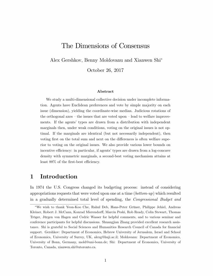
The geometric intuition of the sub-optimality of voting on independent issues is
illustrated in Figure 2 below.
Assume that 0 = µX ≤ mX and 0 = µY ≤ mY . We want to show that a
small rotation improves welfare if f ′X (mX) ≥ 0 and f ′Y (mY ) ≥ 0. Assume that the
unrotated median is B. Therefore, by independence, there is a mass of 50% above the
AC line and a mass of 50% to the right of GH line. Consider a small rotation with
angle θ > 0, so that new axes are x′ and y′. We want to show that this shifts the new
16
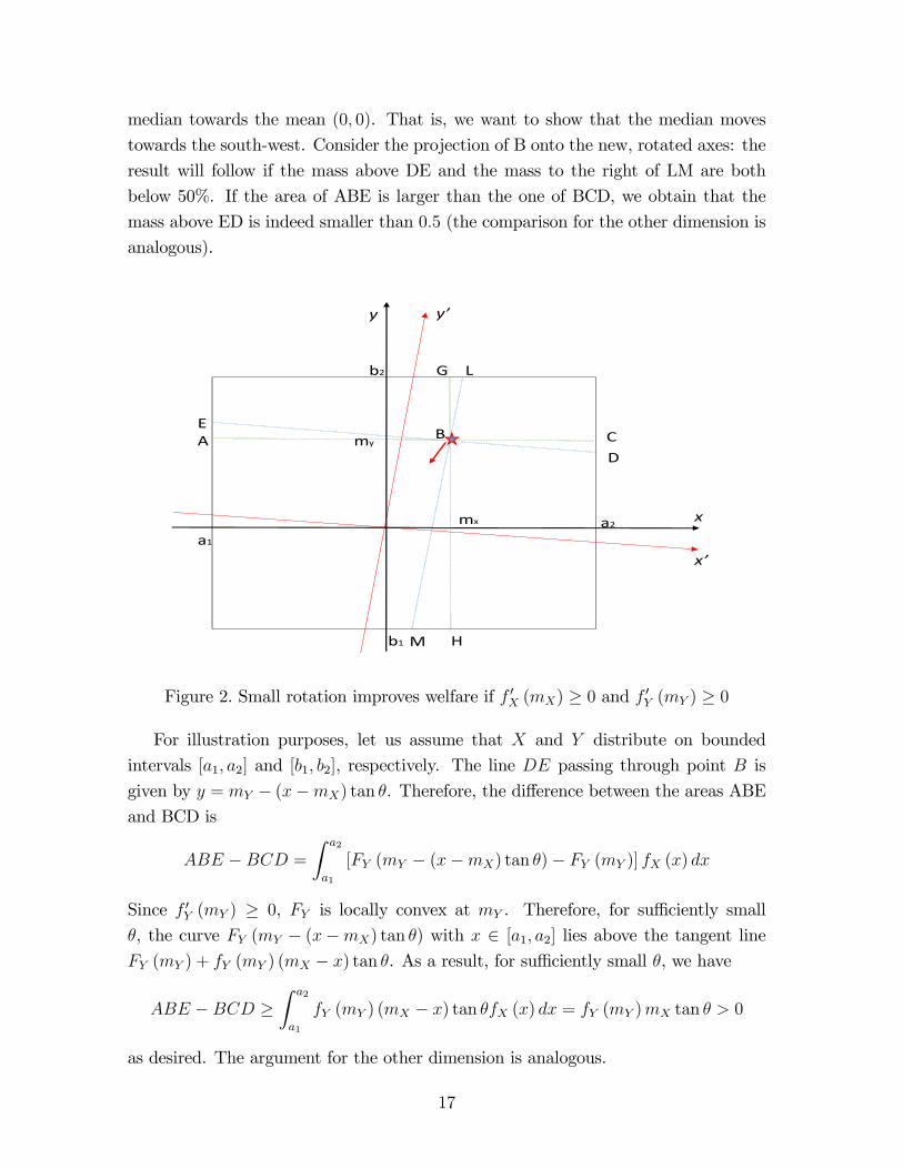
median towards the mean (0, 0). That is, we want to show that the median moves
towards the south-west. Consider the projection of B onto the new, rotated axes: the
result will follow if the mass above DE and the mass to the right of LM are both
below 50%. If the area of ABE is larger than the one of BCD, we obtain that the
mass above ED is indeed smaller than 0.5 (the comparison for the other dimension is
analogous).
my
mx
B CD
b2
a2
y y’
x
x’
AE
H
G L
M
a1
b1
Figure 2. Small rotation improves welfare if f ′X (mX) ≥ 0 and f ′Y (mY ) ≥ 0
For illustration purposes, let us assume that X and Y distribute on bounded
intervals [a1, a2] and [b1, b2], respectively. The line DE passing through point B is
given by y = mY − (x−mX) tan θ. Therefore, the difference between the areas ABE
and BCD is
ABE −BCD =
∫ a2
a1
[FY (mY − (x−mX) tan θ)− FY (mY )] fX (x) dx
Since f ′Y (mY ) ≥ 0, FY is locally convex at mY . Therefore, for suffi ciently small
θ, the curve FY (mY − (x−mX) tan θ) with x ∈ [a1, a2] lies above the tangent line
FY (mY ) + fY (mY ) (mX − x) tan θ. As a result, for suffi ciently small θ, we have
ABE −BCD ≥∫ a2
a1
fY (mY ) (mX − x) tan θfX (x) dx = fY (mY )mX tan θ > 0
as desired. The argument for the other dimension is analogous.
17
An alternative suffi cient condition in Theorem 2 can be formulated in terms of
the familiar order of the mode, median, mean of the distribution. If random variables
X and Y are unimodal,17 then the rotation of θ = 0 is a local utility minimum
as long as the median always lies between the mode and the mean. This alternative
suffi cient condition is simple and intuitive: there are elegant, general characterizations
of distributions where such orders of the mode, median, mean hold (see for example,
Dharmadhikari and Joag-Dev [1988], Basu and DasGupta [1997]).
Corollary 1 Assume that X and Y are unimodal and independent. Suppose also
that X and Y satisfy
MX ≤ mX ≤ µX or µX ≤ mX ≤MX
MY ≤ mY ≤ µY or µY ≤ mY ≤MY
whereM,m, µ are mode, median and mean, respectively. Then the rotation with angle
θ = 0 is a local utility minimum.
Proof. If MX ≤ mX ≤ µX = 0 (where the last equality holds by normalization),
then mX ≤ 0 and f ′(mX) ≤ 0 because mX is to the right of the mode. Hence
mXf′X (mX) ≥ 0. If 0 = µX ≤ mX ≤MX , then mX ≥ 0 and f ′(mX) ≥ 0 because mX
is to the left of the mode. Hence mXf′X (mX) ≥ 0, and analogously for Y .
3.2 When does “Top-Down”Dominate “Bottom-Up”?
In this subsection, we assume that the marginals X and Y are identically (but not
necessarily independently) distributed. By symmetry, the π/4 rotation is a natural
candidate for improving welfare. For θ = π/4 we have(m− (θ)
m+ (θ)
)=
(median (
√22
(X − Y ))
median (√22
(X + Y ))
)=
√2
2
(0
median (X + Y )
)
The last equality follows because median(λZ) = λmedian(Z) for any random variable
Z, and because X − Y is a symmetric random variable, where the median equals themean, normalized here to be zero.
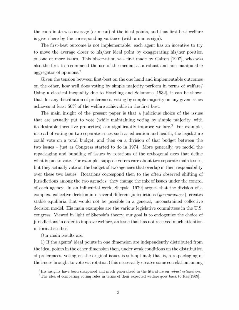
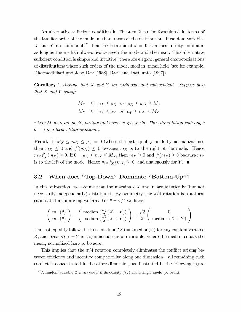
This implies that the π/4 rotation completely eliminates the conflict arising be-
tween effi ciency and incentive compatibility along one dimension —all remaining such
conflict is concentrated in the other dimension, as illustrated in the following figure
17A random variable Z is unimodal if its density f(z) has a single mode (or peak).
18
(assuming mX > µX = 0):
Figure 3. The π/4 rotation with symmetric marginals
The π/4 rotation has the following interpretation: Instead of voting X and Y
separately, the vote is on issues X+Y and X−Y , and the outcome is determined bythe simple majority on each issue. Once voters have decided on X + Y and X − Y ,the planner can then obviously recover X and Y . The two-step voting procedure
associated with π/4 rotation resembles the “top-down”budgeting procedure widely
used in practice: first a total budget is determined, and then it is allocated among
several items.
We now compare the expected utility under the π4rotation with that under the 0
rotation when X and Y are identically distributed. As is also apparent from Figure 3,
this amounts to check whether the original coordinate-wise median vector (mX ,mY ) is
closer to the origin than the new coordinate-wise median vector (mX+Y /2,mX+Y /2),
or vice-versa.
Theorem 3 Suppose X and Y are identically distributed and mX 6= µX . In addition,
suppose that convolution X + Y maintains the relative magnitude of the mean and
median, that is,
mX < (>)µX ⇒ mX+Y < (>)µX+Y .
If mX < (>)µX , and if the median function is super-additive (sub-additive)
mX +mY < (>)mX+Y , (8)
then the expected utility at θ = π4exceeds the expected utility at θ = 0.
19
Proof. Suppose that mX < µX and that µX = 0. The proof for the other case is
completely analogous. By assumption, mX = mY ≤ 0 and m+(π4) ≤ 0. The expected
utility at θ = 0 is
U(0) = −2σ2X − 2m2X
and the expected utility at θ = π4is
U(π
4) = −2σ2X −m2
+(π
4)
Given our assumptions, we have
U(π
4) > U(0)⇔ m+(
π
4) >√
2mX ⇔ m√22(X+Y )
>√
2mX ⇔ mX+Y > 2mX ,
where we use the fact that for any random variable Z, it holds that λmZ = mλZ .
Remark 2 The above suffi cient conditions can also be directly applied to comparethe level of total budget that results from the “bottom-up”and “top-down”budgeting
procedures mentioned in the Introduction.18 Whenever the median function is super
(sub)-additive, the top-down procedure where a total budget is determined first leads
to a higher (lower) overall budget than the bottom-up procedure where votes are item-
by-item and where the total budget is gradually determined.
The super-additivity (or sub-additivity) condition on the median function, though
elegant, may not be easily verified directly since it involves the computation of the
convolution and its median. Assuming that X and Y are I.I.D., we can present a
simple, directly verifiable, suffi cient condition that simultaneously guarantees mX <
(>)µX and mX +mY < (>)mX+Y .
Proposition 1 Suppose that X and Y are I.I.D. and that mX 6= µX . If
FX (mX + ε) + FX (mX − ε) ≤ (≥) 1 for all ε > 0, (9)
then
mX < (>)µX and mX +mY < (>)mX+Y .
Proof. See Appendix A.It is worth noting that van Zwet [1979] shows that the same condition (9) implies
that µX < mX < MX (µX > mX > MX). It follows from Corollary 1 that con-
dition (9) also implies the suffi cient condition in Theorem 2 for zero rotation to be
suboptimal.
18Note that this question is not identical to the question of utility comparisons.
20
We can apply Proposition 1 to show that, if F is either strictly convex or concave,
then the π/4 rotation is strictly better than zero rotation.19
Corollary 2 Suppose that X and Y are I.I.D. and that µX 6= mX . If F (x) is strictly
convex or strictly concave, then the expected utility at θ = π/4 is strictly higher than
the expected utility at θ = 0.
Proof. Note that F (X) is uniformly distributed random variable , so thatE [F (X)] =
1/2. Suppose that F is strictly convex. The concave case can be proved analogously.
By Jensen’s inequality
F (mX) =1
2= E [F (X)] > F (E [X]) = F (µX) .
Hence, mX > µX . In order to show that mX + mY > mX+Y , it is suffi cient to show
that
FX (mX + ε) + FX (mX − ε) ≥ 1 for all ε > 0.
Note that fX (mX + ε)−fX (mX − ε) > 0 by strict convexity of F , so FX (mX + ε)+
FX (mX − ε) is increasing in ε and reaches a minimum at ε = 0. Since FX (mX) +
FX (mX) = 1, we must have FX (mX + ε) + FX (mX − ε) ≥ 1 for all ε > 0.
In Appendix A, we show how the super-additivity condition in Theorem 3 is
satisfied for two well-known families of distributions where condition (9) is not easily
checked, or does not hold. We also show there, by making use of copulas, an example
where independence is not necessary.
Note that the dominance of π/4 does not require the knowledge of the exact
probability distribution of the bliss points. It is enough to know that the distribution
has symmetric marginals and satisfies the required properties. Given the symmetry of
X and Y and the sub-optimality of the zero rotation, the π/4 rotation is the natural
candidate for the optimal rotation. Even though all our numerical simulations clearly
suggest it, we were unable to analytically prove that the π/4 rotation is fully optimal.
But, if X and Y are I.I.D., we can analytically show that the π/4 rotation is a critical
point, i.e., the first-order condition (6) is satisfied when θ = π/4, and numerically show
that the π/4 rotation is indeed optimal for several standard families of distributions.
19Note that, if X has a bounded support (a, b), a suffi cient condition for the case of µX < mX is
FX (mX + ε) + FX (mX − ε) ≥ 1 for all ε ∈ (0, b−mX) .
and a suffi cient condition for the other case is
FX (mX + ε) + FX (mX − ε) ≤ 1 for all ε ∈ (0,mX − a) .
21
Proposition 2 For any I.I.D. marginals X and Y , θ = π/4 is a critical point, i.e.,
it satisfies the first order condition.
Proof. See Appendix A.If we can verify second-order conditions either locally or globally, then Proposition
2 can tell us whether θ = π/4 is local or global utility maximum. Unfortunately, the
second order conditions, evaluated at θ = π/4, turn out to be very elusive.
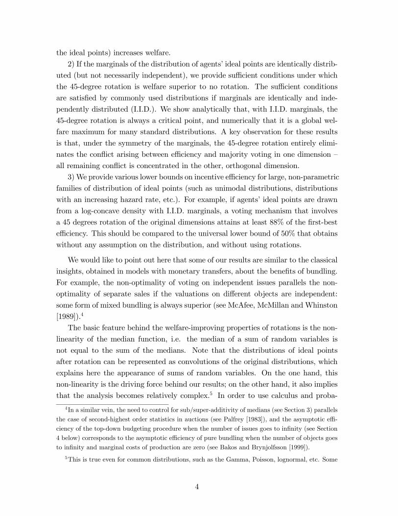
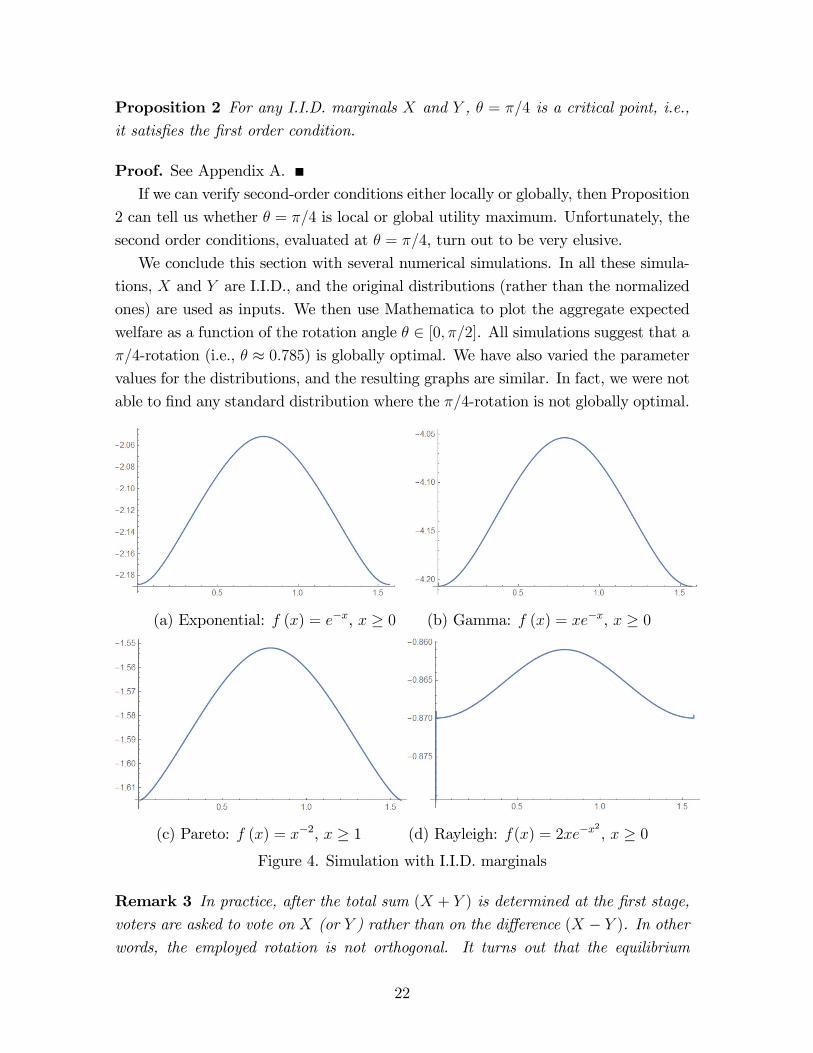
We conclude this section with several numerical simulations. In all these simula-
tions, X and Y are I.I.D., and the original distributions (rather than the normalized
ones) are used as inputs. We then use Mathematica to plot the aggregate expected
welfare as a function of the rotation angle θ ∈ [0, π/2]. All simulations suggest that a
π/4-rotation (i.e., θ ≈ 0.785) is globally optimal. We have also varied the parameter
values for the distributions, and the resulting graphs are similar. In fact, we were not
able to find any standard distribution where the π/4-rotation is not globally optimal.
(a) Exponential: f (x) = e−x, x ≥ 0 (b) Gamma: f (x) = xe−x, x ≥ 0
(c) Pareto: f (x) = x−2, x ≥ 1 (d) Rayleigh: f(x) = 2xe−x2
, x ≥ 0
Figure 4. Simulation with I.I.D. marginals
Remark 3 In practice, after the total sum (X + Y ) is determined at the first stage,
voters are asked to vote on X (or Y ) rather than on the difference (X − Y ). In other
words, the employed rotation is not orthogonal. It turns out that the equilibrium
22
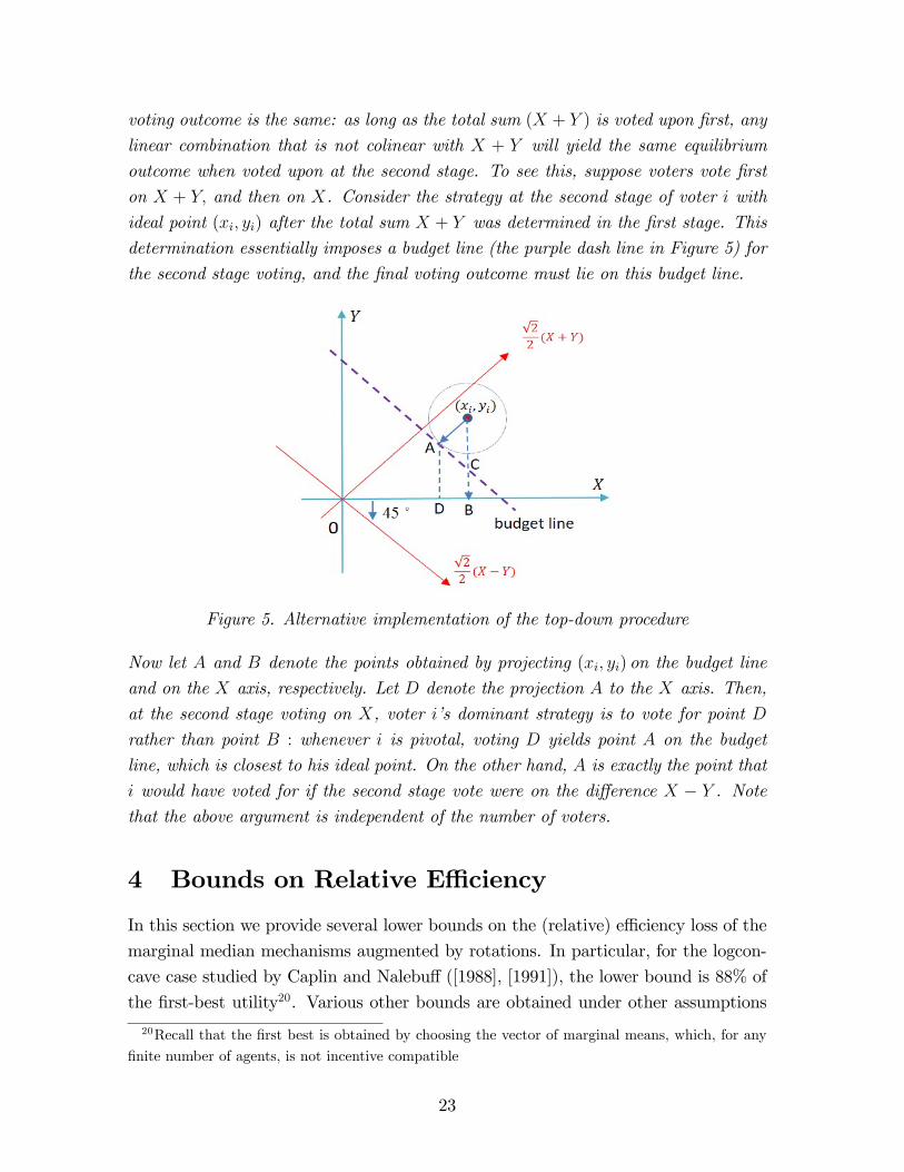
voting outcome is the same: as long as the total sum (X + Y ) is voted upon first, any
linear combination that is not colinear with X + Y will yield the same equilibrium
outcome when voted upon at the second stage. To see this, suppose voters vote first
on X + Y, and then on X. Consider the strategy at the second stage of voter i with
ideal point (xi, yi) after the total sum X + Y was determined in the first stage. This
determination essentially imposes a budget line (the purple dash line in Figure 5) for
the second stage voting, and the final voting outcome must lie on this budget line.
Figure 5. Alternative implementation of the top-down procedure
Now let A and B denote the points obtained by projecting (xi, yi) on the budget line
and on the X axis, respectively. Let D denote the projection A to the X axis. Then,
at the second stage voting on X, voter i’s dominant strategy is to vote for point D
rather than point B : whenever i is pivotal, voting D yields point A on the budget
line, which is closest to his ideal point. On the other hand, A is exactly the point that
i would have voted for if the second stage vote were on the difference X − Y . Notethat the above argument is independent of the number of voters.
4 Bounds on Relative Effi ciency
In this section we provide several lower bounds on the (relative) effi ciency loss of the
marginal median mechanisms augmented by rotations. In particular, for the logcon-
cave case studied by Caplin and Nalebuff ([1988], [1991]), the lower bound is 88% of
the first-best utility20. Various other bounds are obtained under other assumptions
20Recall that the first best is obtained by choosing the vector of marginal means, which, for any
finite number of agents, is not incentive compatible
23
on the distributions governing the distribution of voter’s ideal points. The proofs use
several classical statistical inequalities, and some more recent concentration inequal-
ities.Assume that ideal points are distributed such that the marginals are given by
random variables (X, Y ) where X and Y are not necessarily identical, and are poten-
tially correlated. Since the results heavily use statistical results that establish relations
between the mean, median and variance, we work here with the non-normalizedvariables (so that the role of the mean and its relations to the other statistics does not
get obscured by the normalization we used above). The first-best expected utility,
attained by choosing the mean in each coordinate is given by
−E(X − µX)2 − E(Y − µY )2 = −σ2X − σ2Y .
Note that the first best utility decreases as the variances increase. The expected
utility of rotated medians with angle θ is given by
U (θ) = −σ2X − σ2Y −(µ− (θ)−m− (θ)
)2 − (µ+ (θ)−m+ (θ))2.
Thus, the relative effi ciency of the rotation with angle θ (relative to first best) is given
by:
EF (θ) =σ2X + σ2Y
σ2X + σ2Y +(µ− (θ)−m− (θ)
)2+(µ+ (θ)−m+ (θ)
)2 ≤ 1
Observe that two forces play here a role: on the one hand, a distribution that is
concentrated around a central location (such as the mean or the median) will have
a small difference between mean and median, which tends to increase the relative
effi ciency. On the other hand, such a distribution also has a low variance so that the
difference between mean and median plays a bigger overall role.21
We define the maximal relative effi ciency as
EF ≡ maxθEF (θ) .
The first-best outcome can be attained by majority voting (in the limit with a large
number of agents) if the distributions of both X and Y are symmetric around their
respective means. In this case we have µ− (θ) = m− (θ) and µ+ (θ) = m+ (θ).
Example 2 (Normal Distribution) LetX and Y be independently distributed nor-
mal random variables with zero mean. Then X cos θ − Y sin θ and X sin θ + Y cos θ
are also normally distributed with mean and also median equal to zero. Thus, the
first-best is implementable, and all rotations are welfare equivalent. This proves a
conjecture about the normal distribution due to Kim and Roush [1984].21It is interesting to note that the covariance ofX and Y does not play a direct role in the effi ciency
calculations: it only enters in the way that the medians of the convolutions are calculated.
24

We now obtain various lower bounds on the attained effi ciency for various classes
of distributions. We say that a random variable X has increasing failure rate (IFR)
if its hazard rate f (x) / (1− F (x)) is increasing in x.
Theorem 4 The following relative effi ciency bounds hold:
1. For any random variables X and Y , EF ≥ 12.
2. If both X and Y are unimodal, then EF > 58.
3. If both X and Y have an increasing failure rate (IFR) such that µX ≤ mX and
µY ≤ mY , then EF > 35; if in addition X and Y are I.I.D., then EF ≥ 0.754.
4. If X and Y are identically distributed, then EF ≥ 2σ2X3σ2X+Cov(X,Y )
. Thus, if X
and Y are independent, EF ≥ 23, and in the co-monotonic scenario expected
utility cannot be improved by rotation.
5. If X and Y are I.I.D. and each has a log-concave density, then EF ≥ 0.876.
Proof. 1. A classical inequality due to Hotelling and Solomons [1932] says that thesquare distance between the mean and median of any random variable is always less
than variance:
(µ−m)2 ≤ σ2.
Therefore,(µ− (θ)−m− (θ)
)2 ≤ σ2−(θ) = σ2X cos2 θ + σ2Y sin2 θ − 2 sin θ cos θCov(X, Y )(µ+ (θ)−m+ (θ)
)2 ≤ σ2+(θ) = σ2X sin2 θ + σ2Y cos2 θ + 2 sin θ cos θCov(X, Y )
Hence we obtain the universal bound:
EF (θ) ≥ σ2X + σ2Y2σ2X + 2σ2Y
=1
2
2. For the class of unimodal distributions it can be shown that the squared
distance between mean and median is at most 35variance (see Basu and DasGupta
[1997]). Thus, for such distributions we get:
EF > EF (0) ≥ σ2X + σ2Y(σ2X + σ2Y ) + 3
5(σ2X + σ2Y )
=5
8
3. For the class of distributions with an increasing failure rate (IFR), if µX ≤ mX ,
then we can obtain from Rychlik [2000] that
(µX −mX)2
σ2≤
(− log(12)− 1
2)2
34
+ log(12)
= 0.656,
25
and hence an effi ciency rate of
EF ≥ EF (0) ≥ σ2X + σ2Y(σ2X + σ2Y ) + 0.656(σ2X + σ2Y )
=1
1 + 0.656' 3
5.
If in addition, X and Y are I.I.D., then the convolution of two such variables is again
IFR (see Barlow and Proschan [1965]) and we obtain
EF ≥ EF (π
4) ≥ 2σ2X
2σ2X + 0.65σ2X= 0.754.
4. If X distributes as Y (not necessarily independent), we know that X − Y is
symmetric and hence that m−(π4
)= µ−
(π4
)= 0. This yields:
EF ≥ EF (π
4) =
2σ2X
2σ2X +(µ+(π4
)−m+
(π4
))2 ≥ 2σ2X3σ2X + Cov(X, Y )
Assume that (X1, Y1) and (X2, Y2) belong to the same Frechet class M(F1, F2) of bi-
variate distributions with fixed marginals F1 and F2. Moreover, assume that (X1, Y1)
≤PQD (X2, Y2) where PQD stands for the positive quadrant order (see Lehmann
[1966]). This stochastic order measures the amount of positive dependence of the un-
derlying random vectors.22 We obtain that all one-dimensional variances are identical,
but that Cov(X1, Y1) ≤ Cov(X2, Y2). Thus, the worst case effi ciency bound is higher
when the variates are less positive dependent. In particular, for given marginals, the
highest worst-case effi ciency of the π4rotation is achieved for the I.I.D. case where
Cov(X, Y ) = 0, and where:
EF ≥ EF (π
4) ≥ 2σ2X
3σ2X≥ 2
3
The polar case to independence is the case where X and Y are co-monotonic: then,
their covariance is maximized for given marginals, and, moreover, their convolution
is quantile-additive (see Kaas et al. [2002]). In other words, quantiles and thus
medians (the 50% quantile) are linear functions. Hence we obtain for the median
that m+(π4) =√
2mX , that m2+(π
4) ≤ 2σ2X and hence that
∀θ, EF = EF (π
4) ≥ 2σ2X
4σ2X=
1
2
In the co-monotonic scenario expected utility cannot be improved by rotation.
5. Consider now the I.I.D. case with log-concave densities.23 Then X and Y
are unimodal. Their convolution is log-concave (Prekopa [1973]), and hence also
22It is implied, for example, by the supermodular order.23Note that any log-concave distribution on the plane yields log-concave marginals (Prekopa
[1973]).
26
unimodal.24 Let fX = fY denote the respective logconcave densities. Bobkov and
Ledoux [2014] prove that25
1
12σ2X≤ f 2X(mX) ≤ 1
2σ2X
On the other hand, Ball and Böröczky [2010] prove that:
fX(mX)· | mX − µX |≤ ln
(√e
2
)Combining the two inequalities above yields:
(mX − µX)2 ≤ 1
f 2X(mX)ln2(√
e
2
)≤ 12σ2X ln2
(√e
2
)The effi ciency bound in the log-concave case becomes then:
EF ≥ EF (π
4) ≥ 2σ2X
2σ2X + 12σ2X ln2(√
e2
) =1
1 + 6 ln2(√
e2
) = 0.876.
It is important to note that the above calculations also show that the improve-
ment obtained by rotation may be significant. Just to give one example, consider
the distribution for which the Hotelling-Solomons bound is achieved with equality.26
Then, the second-best welfare in the I.I.D. case without rotation is exactly half of
the first-best welfare, while the welfare following the 45 degree rotation is at least
two-thirds of the original first best, yielding an improvement of at least 30%.
In Appendix B, we show how the above bounds can be obtained for the case of
more dimensions. For example, in the I.I.D, case, the relative effi ciency tends to 1
when the number of dimensions becomes infinite.
5 Concluding Remarks
A re-definition of issues facilitates the search for an optimal consensus among ex-
ante conflicting interests. We have shown that voting by simple majority on each
24The convolution of unimodal densities need not be unimodal ! But, the convolution of X and
Y is unimodal for any Y iffX is log-concave (see Ibragimov [1956])25Interestingly enough, the left hand side of the inequality applies to all probabiliy densities on
the real line.26This is a discrete distribution concentrated on two points. But, it can be easily approximated
by continuous distribution that satisfy the bound with almost equality, for any needed degree of
precision.
27
dimension becomes a highly effi cient aggregation mechanism when combined with
a judicious choice of the issues that are put up for vote. Our study endogenizes
the process by which a “structure induced equilibrium” can be reached in a com-
plex multi-dimensional collective decision problem with incomplete information about
preferences. While we have focused on welfare maximization, other goals (such as
maximizing the utility of an agenda setter) can be analyzed by the same methods. A
companion paper will explore in more detail the case of a finite number of voters.
6 Appendix A: Omitted Proofs
6.1 Proof of Theorem 2
As we noted in the text, in order to show that θ = 0 is suboptimal, it is suffi cient to
show
m−(0)m′−(0) +m+(0)m′+(0) = 0, (10)
and
m′′−(0)m−(0) + (m′−(0))2 +m′′+(0)m+(0) + (m′+(0))2 < 0. (11)
: 2m′2+2m′′<0.0By definition of m+ (θ), we note that
1
2= FX sin θ+Y cos θ (m+ (θ))
=
∫ ∞−∞
Pr
(Y <
m+ (θ)− x sin θ
cos θ
)fX (x) dx
=
∫ ∞−∞
FY
(m+ (θ)− x sin θ
cos θ
)fX (x) dx
Since it holds for all θ, we take a derivative with respect to θ to obtain
0 =
∫ ∞−∞
fY
(m+ (θ)− x sin θ
cos θ
)(m′+ (θ) cos θ − x+m+ (θ) sin θ
cos2 θ
)fX (x) dx (12)
By taking the second derivative with respect to θ, we obtain
0 =
∫ ∞−∞
f ′Y
(m+ (θ)− x sin θ
cos θ
)(m′+ (θ) cos θ − x+m+ (θ) sin θ
cos2 θ
)2fX (x) dx
+
∫ ∞−∞
fY
(m+(θ)−x sin θ
cos θ
)cos4 θ
( [m′′+ (θ) cos θ +m+ (θ) cos θ
]cos2 θ
+2 cos θ sin θ(m′+ (θ) cos θ − x+m+ (θ) sin θ
) ) fX (x) dx
(13)
28
If θ = 0, then conditions (12) and (13) reduce to
0 =
∫ ∞−∞
fY (m+ (0))(m′+ (0)− x
)fX (x) dx
and
0 =
∫ ∞−∞
f ′Y (m+ (0))(m′+ (0)− x
)2fX (x) dx+
∫ ∞−∞
fY (m+ (0))(m′′+ (0) +m+ (0)
)fX (x) dx
Note that m+ (0) = mY , so that we have
m′+ (0) =fY (mY )
∫∞−∞ xfX (x) dx
fY (mY )∫∞−∞ fX (x) dx
= µX = 0,
and
m′′+ (0) = −mY −f ′Y (mY )
fY (mY )
∫ ∞−∞
x2fX (x) dx.
Similarly, we can write
1
2= FX cos θ−Y sin θ (m− (θ)) =
∫ ∞−∞
FX
(m− (θ) + y sin θ
cos θ
)fY (y) dy
Taking the derivative with respect to θ, we obtain
0 =
∫ ∞−∞
fX
(m− (θ) + y sin θ
cos θ
)(m′− (θ) cos θ + y +m− (θ) sin θ
cos2 θ
)fY (y) dy (14)
Taking the second derivative with respect to θ, we obtain
0 =
∫ ∞−∞
f ′X
(m− (θ) + y sin θ
cos θ
)(m′− (θ) cos θ + y +m− (θ) sin θ
cos2 θ
)2fY (y) dy
+
∫ ∞−∞
fX
(m−(θ)+y sin θ
cos θ
)cos4 θ
( [m′′− (θ) cos θ +m− (θ) cos θ
]cos2 θ
+2 cos θ sin θ[m′− (θ) cos θ + y +m− (θ) sin θ
] ) fY (y) dy
If θ = 0, then the above two conditions reduce to
0 =
∫ ∞−∞
fX (m− (0))(m′− (0) + y
)fY (y) dy
and
0 =
∫ ∞−∞
f ′X (m− (0))(m′− (0) + y
)2fY (y) dy+
∫ ∞−∞
fX (m− (0))(m′′− (0) +m− (0)
)fY (y) dy
Since m− (0) = mX , we have
m′− (0) = −∫∞−∞ yfY (y) dy∫∞−∞ fY (y) dy
= −µY = 0
29
and
m′′− (0) = −mX −f ′X (mX)
fX (mX)
∫ ∞−∞
y2fY (y) dy
Therefore, the first-order condition (10) holds because m′− (0) = m′+ (0) = 0. For
the second order condition (11), note that
m′′−(0)m−(0) + (m′−(0))2 +m′′+(0)m+(0) + (m′+(0))2
= mX
(−mX −
f ′X (mX)
fX (mX)
∫ ∞−∞
y2fY (y) dy
)+mY
(−mY −
f ′Y (mY )
fY (mY )
∫ ∞−∞
x2fX (x) dx
)= −m2
X −m2Y −mX
f ′X (mX)
fX (mX)
∫ ∞−∞
y2fY (y) dy −mYf ′Y (mY )
fY (mY )
∫ ∞−∞
x2fX (x) dx
As a result, condition (11) is equivalent to
m2X +m2
Y +mXf ′X (mX)
fX (mX)
∫ ∞−∞
y2fY (y) dy +mYf ′Y (mY )
fY (mY )
∫ ∞−∞
x2fX (x) dx > 0.
Therefore, a suffi cient condition for the sub-optimality of zero rotation is
mXf′X (mX) ≥ 0,mY f
′Y (mY ) ≥ 0 and m2
X +m2Y 6= 0.
6.2 Proof of Proposition 1
Suppose FX (mX + ε) + FX (mX − ε) ≤ 1 for all ε > 0. The other case is completely
analogous. We first use an argument by van Zwet [1979] to claim that mX < µX .
Note that
mX − µX =
∫ mX
−∞(mX − x) fX (x) dx+
∫ ∞mX
(mX − x) fX (x) dx
=
∫ mX
−∞FX (x) dx−
∫ ∞mX
(1− FX (x)) dx
=
∫ ∞0
[FX (mX − x) + FX (mX + x)− 1] dx
It follows frommX 6= µX thatmX < µX , and that FX (mX − x)+FX (mX + x)−1 <
0 for some interval of x. Next, we use an argument adapted from Watson and Gordon
[1986] to prove that the median function is super-additive. The super-additivity of
the median function is equivalent to
Pr (X + Y < mX +mY ) <1
2(15)
30
Note that
Pr (X + Y < mX +mY )
=
∫ ∞mY
∫ mX+mY −y
−∞fX (x) fY (y) dxdy +
∫ mY
−∞
∫ mX
−∞fX (x) fY (y) dxdy
+
∫ ∞mX
∫ mX+mY −x
−∞fX (x) fY (y) dxdy
=
∫ ∞mY
FX (mX +mY − y) fY (y) dy +1
4+
∫ ∞mX
fX (x)FY (mX +mY − x) dx
=
∫ ∞0
FX (mX − ε) fY (mY + ε) dε+
∫ ∞0
fX (mX + ε)FY (mY − ε) dε+1
4
Therefore, condition (15) is equivalent to
4
∫ ∞0
FX (mX − ε) fY (mY + ε) dε+ 4
∫ ∞0
fX (mX + ε)FY (mY − ε) dε < 1 (16)
Let us define non-negative random variables X+, X−, Y +, Y − as
X+ = X −mX |X ≥ mX and X− = mX −X|X ≤ mX
Y + = Y −mY |Y ≥ mY and Y − = mY − Y |Y ≤ mY
Then
Pr(X− > Y +
)=
∫ ∞0
2FX (mX − ε) 2fY (mX + ε) dε
Pr(Y − > X+
)=
∫ ∞0
2FY (mX − ε) 2fX (mX + ε) dx
Therefore, condition (16) is equivalent to
Pr(X− > Y +
)+ Pr
(Y − > X+
)< 1 (17)
A suffi cient condition for (17) is
Pr(X+ < ε
)≤ Pr
(X− < ε
)and Pr
(Y + < ε
)≤ Pr
(Y − < ε
)(18)
for all ε > 0 , and with strict inequality for some open interval of ε, because by setting
ε = Y + and ε = X+, respectively, we obtain
Pr(X+ < Y +
)< Pr
(X− < Y +
)and Pr
(Y + < X+
)< Pr
(Y − < X+
)and thus (17). Since X and Y are I.I.D., the suffi cient condition (18) reduces to
Pr(X+ < ε
)≤ Pr
(X− < ε
)for all ε > 0.
31

Equivalently,
Pr (X −mX < ε) ≤ Pr (mX −X < ε) .
which simplifies into the first inequality in (9). As we argued above, since mX 6= µX ,
we must have FX (mX − ε) + FX (mX + ε) − 1 < 0 for some open interval of ε, as
desired.
6.3 Proof of Proposition 2
If X and Y are iid, then we have
m− (π/4) = 0 and m+ (π/4) =
√2
2mX+Y .
Therefore, θ = π/4 is a critical point if
0 = m− (π/4)m′− (π/4) +m+ (π/4)m′+ (π/4) =
√2
2mX+Ym
′+ (π/4)
Recall (12) from the proof of Theorem 2 that
0 =
∫ ∞−∞
fY
(m+ (θ)− x sin θ
cos θ
)(m′+ (θ) cos θ − x+m+ (θ) sin θ
cos2 θ
)fX (x) dx
Hence, if X and Y are IID and θ = π/4, we have
0 =
∫ ∞−∞
f(√
2m+ (π/4)− x)(√
2m′+ (π/4)− 2x+√
2m+ (π/4))f (x) dx
It follows that√
2m′+ (π/4) fX+Y
(√2m+ (π/4)
)=
∫ ∞−∞
f(√
2m+ (π/4)− x)(
2x−√
2m+ (π/4))f (x) dx.
Note that by change of variable y =√
2m+ (π/4)− x, we have∫ ∞−∞
f ′(√
2m+ (π/4)− x)(
2x−√
2m+ (π/4))2f (x) dx
=
∫ ∞−∞
f ′ (y)(
2y −√
2m+ (π/4))2f (y) dy.
Therefore,
0 =
∫ ∞−∞
[f ′(√
2m+ (π/4)− x)f (x)− f ′ (x) f
(√2m+ (π/4)− x
)](2x−
√2m+ (π/4)
)2dx
=
[f(√
2m+ (π/4)− x)f (x)
(2x−
√2m+ (π/4)
)2]∞−∞
−∫ ∞−∞
f(√
2m+ (π/4)− x)f (x) 4
(2x−
√2m+ (π/4)
)dx
= 4√
2m′+ (π/4) fX+Y
(√2m+ (π/4)
)32
where we assume that
limx→∞
f(√
2m+ (π/4)− x)f (x)
(2x−
√2m+ (π/4)
)2= lim
x→−∞f(√
2m+ (π/4)− x)f (x)
(2x−
√2m+ (π/4)
)2= 0.
Therefore, m′+ (π/4) = 0. It follows that√
2mX+Ym′+ (π/4) = 0, so θ = π/4 is indeed
a critical point.
6.4 Examples for Section 3.2
We show here how the super-additivity condition in Theorem 3 is satisfied for two
well-known families of distributions where condition (9) is not easily checked, or does
not hold.27 This requires a few definitions and some results that use majorization
and Schur-convexity arguments.
Definition 1 A vector (a, b) is said to majorize (a′, b′), written as (a, b) � (a′, b′), if
a+ b = a′+ b′ and if max(a, b) > max {a′, b′}. A function h (a, b) is said to be Schur-
convex in (a, b) if h (a′′, b′′) ≥ h (a′, b′) whenever (a′′, b′′) � (a′, b′), and Schur-concave
in (a, b) if h (a′′, b′′) ≤ h (a′, b′) whenever (a′′, b′′) � (a′, b′).
Consider first the large and important family of Gamma distributions with density
fα,β (x) =βα
Γ (α)xα−1e−βx for x > 0.
This family contains the Exponential (that can be obtained by setting α = 1) and
many other well known distributions. For any constant c > 0, the random variable
cX is also Gamma with parameters α and β/c. If X and Y are independent Gamma
with parameters (αX , β) and (αY , β), respectively, then X + Y is also Gamma with
parameters (αX +αY , β). Thus, the Gamma family is closed under scaling and under
convolution. In a classic study, Bock et al. [1987] showed that Pr (aX + bY ≤ t),
0 ≤ a, b ≤ 1, is Schur-convex in (a, b) for all t ≤ µX . Since (1, 0) �(12, 12
), we have
F 12X+ 1
2Y (t) ≤ FX(t) for all t ≤ mX . This implies m 1
2X+ 1
2Y ≥ mX as desired.28
27Although the super-additivity (or sub-additivity) condition is derived for normalized distribu-
tions, it is straightward to verify that it is also suffi cient for original distributions.28Alternatively, let m(α, β) denote the median of Gamma random variable X with parameters α
and β. Then m(α, β) = m(α, 1)/β. Note that
U(π
4) = −2σ2 (α, β)−
(µ+ −m+
)2= −2σ2 (α, β)−
(√2α
β−√2
2βm(2α, 1)
)2= −2σ2 (α, β)− 1
2β2(2α−m(2α, 1))2
33
A second family is the Rayleigh distribution with cumulative distribution
F (x) = 1− e−x2 for x ≥ 0.
Suppose X, Y are I.I.D. distributed according to Rayleigh.29 Then, according to
Lemma 4 in Hu and Lin [2000], we have
Pr (X cos θ + Y sin θ ≤ z) = 1−∫ π/2
0
sin(2τ)(1 + φ2(θ, τ , z)
)e−φ
2(θ,τ ,z)dτ
where φ(θ, τ , z) = z/ cos(θ − τ). The medians of X and of Y are mX = mY =√
ln 2.
It can be (numerically) verified that
Pr(
(X + Y ) /√
2 ≤√
2mX
)= 1−
∫ π/2
0
sin(2τ)(
1 + φ2(π
4, τ ,√
2 ln 2))e−φ
2(π4,τ ,√2 ln 2)dτ
≈ 0.4658
< 0.5
= Pr(
(X + Y ) /√
2 ≤ m+(π
4))
where the last equality follows from the definition of m+(π4). Hence, m+(π
4) >√
2mX
as desired.
By assuming independence between X and Y , we were able to derive operational,
suffi cient conditions for the π/4 rotation to dominate the zero rotation, but indepen-
dence is not necessary. We now present an example where, even though X and Y are
correlated, the median function is super-additive (sub-additive) so the π/4 rotation
is welfare superior to the zero rotation. The standard tool we use to model corre-
lation between X and Y for given marginals is the copula (see Nelson [2006] for an
introduction).
and
U(0) = −2σ2(α, β)− 2 (µX −mX)2= −2σ2(α, β)− 2
β2(α−m(α, 1))2
Therefore,
U(π
4) > U (0) ⇔ 1
2β2(2α−m(2α, 1))2 < 2
β2(α−m(α, 1))2
⇔ (2α−m(2α, 1))2 < 4(α−m(α, 1))2
⇔ m2(2α, 1)− 4αm(2α, 1) < 4m2(α, 1)− 8αm(α, 1)⇔ m(2α, 1) > 2m(α, 1)
The last inequality holds because, as shown in Berg and Pedersen [2008], m(α, 1) is convex in α.29If Z1, Z2 is a random sample of size 2 from a normal distribution N(0, 1) then the distribution
of X =√Z21 + Z
22 is Rayleigh. In other words, the Rayleigh is the distribution of the norm of a
two-dimensional random vector whose coordinates are normally distributed.
34
Example 3 Suppose that X and Y are identically distributed on [0, 1] with marginals
FX (x) = x2 and FY (y) = y2. To model correlation between X and Y , we consider
here the Farlie-Gumbel-Morgenstern (FGM) copula
Cδ (p, q) = pq + δpq (1− p) (1− q)
with p, q ∈ [0, 1] and δ ∈ [−1, 1]. The correlation coeffi cient for FGM copula is
ρ = δ/3 ∈ [−1/3, 1/3]. It follows from the Sklar theorem that we can write the joint
distribution F (x, y) in terms of its marginals and a copula C (p, q):
F (x, y) = C (FX (x) , FY (y)) .
With some algebra, we can derive the joint density as
f (x, y) = 4xy + 4δxy(2x2 − 1
) (2y2 − 1
).
Therefore, as in the proof of Proposition 1, we can write Pr (X + Y < mX +mY ) as
2
∫ 1
mY
∫ mX+mY −y
0
f (x, y) dxdy +
∫ mY
0
∫ mX
0
f (x, y) dxdy
= 2
∫ 1
√2/2
∫ √2−y0
(4xy + 4δxy
(2x2 − 1
) (2y2 − 1
))dxdy
+
∫ √2/20
∫ √2/20
(4xy + 4δxy
(2x2 − 1
) (2y2 − 1
))dxdy
=
(146
35− 104
35
√2
)δ − 8
3
√2 +
13
3> 0.5
for all δ ∈ [−1, 1]. Consequently, we have mX+Y < mX + mY . Since FX (x) = x2
is convex, µX < mX . Hence, the suffi cient condition (8) in Theorem 3 is fulfilled.
Alternatively, suppose FX (x) =√x and FY (y) =
√y. If we again restrict attention
to the FGM copula, we can follow the same procedure to show that mX+Y > mX +mY
and µX > mX .
7 Appendix B: More than Two Dimensions
In this appendix, we illustrate how to generalize our main results (Theorems 2-4) to
higher dimensions. Consider K independent issues, denoted by Xk, k = 1, ..., K. We
writeX = (X1, ..., XK)T and assume that all random variablesXk are normalized. Let
SOK denote the special orthogonal group in dimension K which consists of K × K
35
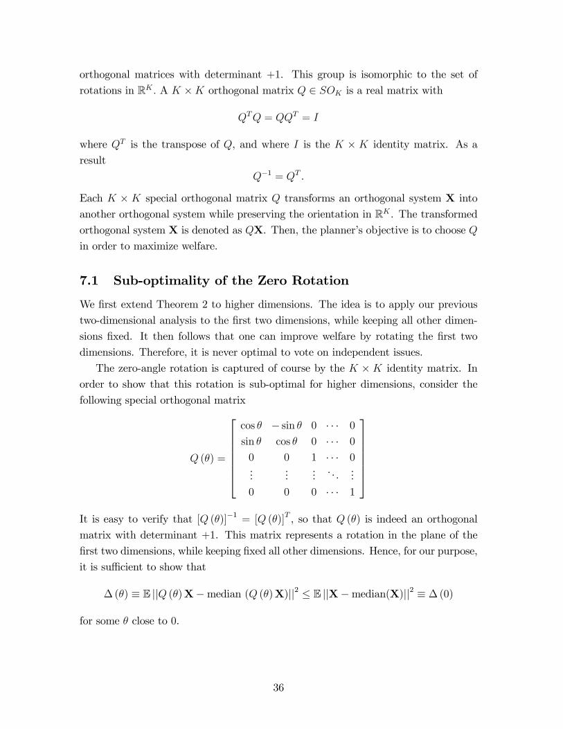
orthogonal matrices with determinant +1. This group is isomorphic to the set of
rotations in RK . A K ×K orthogonal matrix Q ∈ SOK is a real matrix with
QTQ = QQT = I
where QT is the transpose of Q, and where I is the K × K identity matrix. As a
result
Q−1 = QT .
Each K × K special orthogonal matrix Q transforms an orthogonal system X into
another orthogonal system while preserving the orientation in RK . The transformedorthogonal system X is denoted as QX. Then, the planner’s objective is to choose Q
in order to maximize welfare.
7.1 Sub-optimality of the Zero Rotation
We first extend Theorem 2 to higher dimensions. The idea is to apply our previous
two-dimensional analysis to the first two dimensions, while keeping all other dimen-
sions fixed. It then follows that one can improve welfare by rotating the first two
dimensions. Therefore, it is never optimal to vote on independent issues.
The zero-angle rotation is captured of course by the K ×K identity matrix. In
order to show that this rotation is sub-optimal for higher dimensions, consider the
following special orthogonal matrix
Q (θ) =
cos θ − sin θ 0 · · · 0
sin θ cos θ 0 · · · 0
0 0 1 · · · 0...
....... . .
...
0 0 0 · · · 1
It is easy to verify that [Q (θ)]−1 = [Q (θ)]T , so that Q (θ) is indeed an orthogonal
matrix with determinant +1. This matrix represents a rotation in the plane of the
first two dimensions, while keeping fixed all other dimensions. Hence, for our purpose,
it is suffi cient to show that
∆ (θ) ≡ E ||Q (θ)X−median (Q (θ)X)||2 ≤ E ||X−median(X)||2 ≡ ∆ (0)
for some θ close to 0.
36
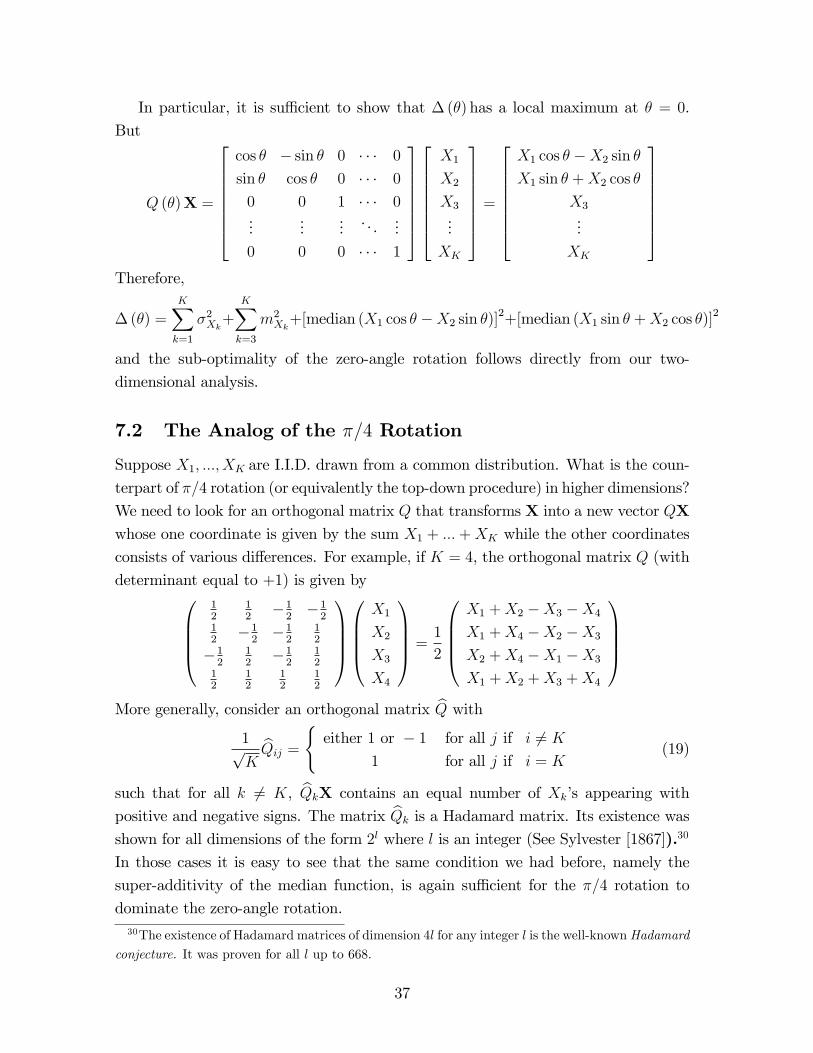
In particular, it is suffi cient to show that ∆ (θ) has a local maximum at θ = 0.
But
Q (θ)X =
cos θ − sin θ 0 · · · 0
sin θ cos θ 0 · · · 0
0 0 1 · · · 0...
....... . .
...
0 0 0 · · · 1
X1
X2
X3
...
XK
=
X1 cos θ −X2 sin θ
X1 sin θ +X2 cos θ
X3
...
XK
Therefore,
∆ (θ) =K∑k=1
σ2Xk+
K∑k=3
m2Xk
+[median (X1 cos θ −X2 sin θ)]2+[median (X1 sin θ +X2 cos θ)]2
and the sub-optimality of the zero-angle rotation follows directly from our two-
dimensional analysis.
7.2 The Analog of the π/4 Rotation
Suppose X1, ..., XK are I.I.D. drawn from a common distribution. What is the coun-
terpart of π/4 rotation (or equivalently the top-down procedure) in higher dimensions?
We need to look for an orthogonal matrix Q that transforms X into a new vector QX
whose one coordinate is given by the sum X1 + ...+XK while the other coordinates
consists of various differences. For example, if K = 4, the orthogonal matrix Q (with
determinant equal to +1) is given by12
12−12−12
12−12−12
12
−12
12−12
12
12
12
12
12
X1
X2
X3
X4
=1
2
X1 +X2 −X3 −X4
X1 +X4 −X2 −X3
X2 +X4 −X1 −X3
X1 +X2 +X3 +X4
More generally, consider an orthogonal matrix Q with
1√KQij =
{either 1 or − 1 for all j if i 6= K
1 for all j if i = K(19)
such that for all k 6= K, QkX contains an equal number of Xk’s appearing with
positive and negative signs. The matrix Qk is a Hadamard matrix. Its existence was
shown for all dimensions of the form 2l where l is an integer (See Sylvester [1867]).30
In those cases it is easy to see that the same condition we had before, namely the
super-additivity of the median function, is again suffi cient for the π/4 rotation to
dominate the zero-angle rotation.30The existence of Hadamard matrices of dimension 4l for any integer l is the well-known Hadamard
conjecture. It was proven for all l up to 668.
37
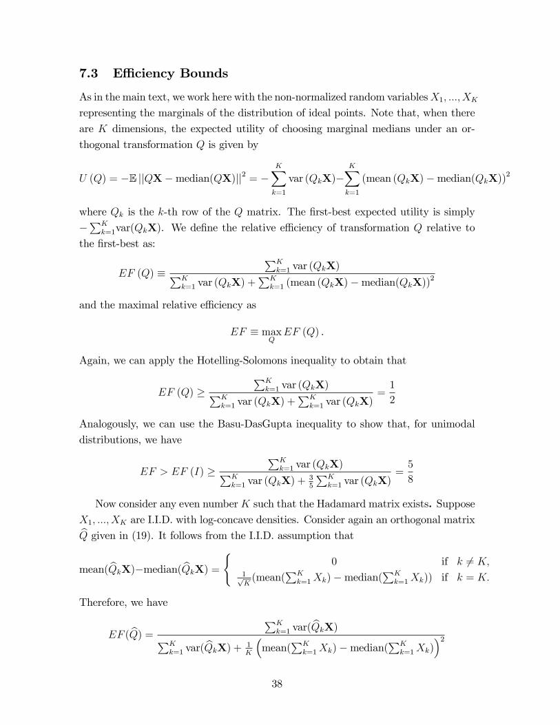
7.3 Effi ciency Bounds
As in the main text, we work here with the non-normalized random variablesX1, ..., XK
representing the marginals of the distribution of ideal points. Note that, when there
are K dimensions, the expected utility of choosing marginal medians under an or-
thogonal transformation Q is given by
U (Q) = −E ||QX−median(QX)||2 = −K∑k=1
var (QkX)−K∑k=1
(mean (QkX)−median(QkX))2
where Qk is the k-th row of the Q matrix. The first-best expected utility is simply
−∑K
k=1var(QkX). We define the relative effi ciency of transformation Q relative to
the first-best as:
EF (Q) ≡∑K
k=1 var (QkX)∑Kk=1 var (QkX) +
∑Kk=1 (mean (QkX)−median(QkX))2
and the maximal relative effi ciency as
EF ≡ maxQ
EF (Q) .
Again, we can apply the Hotelling-Solomons inequality to obtain that
EF (Q) ≥∑K
k=1 var (QkX)∑Kk=1 var (QkX) +
∑Kk=1 var (QkX)
=1
2
Analogously, we can use the Basu-DasGupta inequality to show that, for unimodal
distributions, we have
EF > EF (I) ≥∑K
k=1 var (QkX)∑Kk=1 var (QkX) + 3
5
∑Kk=1 var (QkX)
=5
8
Now consider any even numberK such that the Hadamard matrix exists. SupposeX1, ..., XK are I.I.D. with log-concave densities. Consider again an orthogonal matrix
Q given in (19). It follows from the I.I.D. assumption that
mean(QkX)−median(QkX) =
{0 if k 6= K,
1√K
(mean(∑K
k=1Xk)−median(∑K
k=1Xk)) if k = K.
Therefore, we have
EF (Q) =
∑Kk=1 var(QkX)∑K
k=1 var(QkX) + 1K
(mean(
∑Kk=1Xk)−median(
∑Kk=1Xk)
)238
Given that X1, ..., XK have log-concave densities, the convolution Z ≡∑K
k=1Xk
also has a log-concave densities. Then the inequalities of Bobkov and Ledoux [2014]
and of Ball and Böröczky [2010] together imply
(mZ − µZ)2 ≤ 1
f 2Z(mZ)ln2(√
e
2
)≤ 12σ2Z ln2
(√e
2
)Hence,
EF (Q) ≥∑K
k=1 var(QkX)∑Kk=1 var(QkX) + 1
K12σ2Z ln2
(√e2
)Let σ2Xk denote the variance of Xk. Then we have σ2Z = Kσ2Xk and
var(QkX) = QkQTk σ
2Xk
= σ2Xk
since QkQTk = 1 by the definition of an orthogonal matrix. Therefore, we obtain the
following effi ciency bound for log-concave densities
EF ≥ EF (Q) ≥Kσ2Xk
Kσ2Xk + 12σ2Xk ln2(√
e2
) =1
1 + 1K
12 ln2(√
e2
)For example, if K = 4, the bound is 93.4%. Note that this bound is increasing the
number of dimensions K, and tends to 100% when K goes to infinity.
Remark 4 More generally, consider any I.I.D. random variables X1, ..., XK with
finite means and variances and consider K such that the Hadamard matrix exists.
Then, for the analog of the π/4 rotation we obtain that
EF ≥ EF (Q) =Kσ2Xk
Kσ2Xk + 1K
(mean(∑K
k=1Xk)−median(∑K
k=1Xk))2
=σ2Xk
σ2Xk + 1K2 (mean(
∑Kk=1Xk)−median(
∑Kk=1Xk))2
→ 1 as K →∞
where the last assertion follows from the central limit theorem.
References
[2012] Ahn, D. and S. Oliveros (2012), "Combinatorial Voting," Econometrica 80(1),89—141.
[2005] Austen-Smith D. and J.S. Banks (2005), Positive Political Theory II: Strategy
and Structure, The University of Michigan Press, Ann Arbor, MI.
39
[1966] Bahadur, R. R. (1966), “A Note on Quantiles in Large Samples,”Annals of
Mathematical Statistics 37(3), 577-580.
[1999] Bakos, Y. and E. Brynjolfsson (1999), “Bundling Information Goods: Pricing,
Profits, and Effi ciency,”Management Science 45(12), 1613-1630.
[2010] Ball, Keith M., and Karoly J. Boroczky (2010), “Stability of the Prekopa-
Leindler Inequality,”Mathematika 56, 339-356.
[1993] Barbera, S., Gul, F. and Stacchetti, E. (1993), “Generalized Median Voter
Schemes and Committees,”Journal of Economic Theory 61(2): 262-289.
[1965] Barlow, R. E., and F. Proschan (1965), Mathematical Theory of Reliability, J.
Wiley & Sons. SIAM, Philadelphia, PA.
[1997] Basu, S. and A. DasGupta (1997), “The Mean, Median, andMode of Unimodal
Distributions: A Characterization,”Theory Probab. Appl., 41(2), 210—223.
[2002] Battaglini, M. (2002), “Multiple Referrals and Multidimensional Cheap Talk,”
Econometrica 70(4), 1379-1401.
[2008] Berg, Christian, and Henrik L. Pedersen (2008), “Convexity of the Median in
the Gamma Distribution,”Ark. Mat. 46, 1—6.
[1948] Black, D. (1948), “On the Rationale of Group Decision-Making,”Journal of
Political Economy 56(1), 23-34.
[1987] Bock M. E., P. Diaconis, F. W. Huffer and M. D. Perlman (1987), “Inequalities
for Linear Combinations of Gamma Random Variables,”Canadian Journal of
Statistics 15 (4), 387-395.
[2014] Bobkov, S. G., and Ledoux, M. (2014), “One-dimensional Empirical Measures,
Order Statistics and Kantorovich Transport Distances,”working paper, Uni-
versity of Minesota.
[1983] Border, Kim C., and J. S. Jordan (1983), “Straightforward Elections, Una-
nimity and Phantom Voters,”Review of Economic Studies 50(1), 153-170.
[1943] Bowen, H. (1943), “The Interpretation of Voting in the Allocation of Economic
Resources,”The Quarterly Journal of Economics 58(1), 27-48.
[1988] Caplin, Andrew, and Barry Nalebuff (1988), “On 64%-Majority Rule,”Econo-
metrica 56(4), 787-814.
40
[1991] Caplin, Andrew, and Barry Nalebuff (1991), “Aggregation and Social Choice,”
Econometrica 59(1), 1-23.
[2007] Charkraborty, A. and R. Harbaugh (2007), “Comparative Cheap Talk,”Jour-
nal of Economic Theory 132, 70-94.
[1988] Dharmadhikari,S., and Kumar, J. (1988), Unimodality, Convexity, and Appli-
cations, Academic Press, First Edition.
[1988] Feld, S. and Grofman, B. (1988), “Majority Rule Outcomes and the Structure
of Debate in One-Issue at a Time Decision-Making,”Public Choice 59, 239-252.
[1987] Ferejohn, J. and Krehbiel, K. (1987), “The Budget Process and the Size of the
Budget,”American Journal of Political Science 31(2), 296-320.
[1907] Galton, F. (1907), “Vox Populi,”first published in Nature 75, 450-451, 1949
[2016] Gershkov, A., Moldovanu, B. and Shi, X. (2016), “Optimal Voting Rules,”
Review of Economic Studies, forthcoming.
[1951] Gil-Pelaez, J. (1951), “Note on the Inversion Theorem,”Biometrika 38 (3-4):481-482.
[1948] Haldane, J.B.S. (1948), “Note on the Median of a Multivariate Distribution,”
Biometrika 35, 414-415.
[1932] Hotelling, Harold, and Leonard M. Solomons (1932), “The Limits of a Measure
of Skewness,”Annals of Mathematical Statistics 3(2), 141-142.
[2000] Hu, Chin-Yuan, and Gwo Dong Lin (2000), “On an Inequality for the Rayleigh
Distribution,”Sankhya: The Indian Journal of Statistics 62(1), 36-39.
[2001] Hu, Chin-Yuan, and Gwo Dong Lin (2001), “An Inequality for the Weighted
Sums of Pairwise I.I.D. Generalized Rayleigh Random Variables,”Journal of
Statistical Planning and Inference 92, 1-5.
[1956] Ibragimov, J. A. (1956). "On the Composition of Unimodal Distributions".
Teoriya Veroyatnostey I, 283-288.
[2002] Kaas, R., Dhaene, J., Vyncke, D., Goovaerts, M.J., and Denuit, M. (2002),
“A Simple Geometric Proof that Comonotonc Risks Have the Convex-Largest
Sum,”Astin Bulletin 32(1), 71-80.
41
[1984] Kim, K. H. and F. W. Roush (1984), “Nonmanipulation in Two Dimensions,”
Mathematical Social Sciences 8, 29-43.
[2016] Kleiner, A. and Moldovanu, B. (2016), “Content Based Agendas and Qualified-
Majorities in Sequential Voting,”American Economic Review, forthcoming.
[1972] Kramer, G. (1972), “Sophisticated Voting over Multidimensional Choice
Spaces,”Journal of Mathematical Sociology 2, 165-180.
[1973] Kramer, G. (1973), “On a Class of Equilibrium Conditions for Majority Rule,”
Econometrica 41(2), 285-297.
[1966] Lehmann, E. (1966), “Some Concepts of Dependence,”Annals of Mathematical
Statistics 37(5), 1137-1153.
[1980] Moulin, H. (1980), “On Strategy-Proofness and Single Peakedness,” Public
Choice 35, 437-455.
[1989] McAfee, P. ,J. McMillan and M. Whinston (1989): “Multiproduct Monopoly,
Commodity Bundling, and Correlation of Values,”Quarterly Journal of Eco-
nomics 104(2), 371-383.
[2006] Nelsen, R.B. (2006), An Introduction to Copulas, second edition, Springer,
New York.
[1983] Palfrey, T. (1983) “Bundling Decisions by a Multiproduct Monopolist with
Incomplete Information,”Econometrica 51(2), 463-483.
[1992] Peters, H., H. van der Stel, and T. Storcken (1992), “Pareto Optimal-
ity, Anonymity, and Strategy-Proofness in Location Problems,”International
Journal of Game Theory 21, 221-235.
[1999] Poterba, J. M. and von Hagen, J. (eds), Fiscal Institutions and Fiscal Peror-
mance, University of Chicago Press, Chiacgo.
[1973] Prekopa, A. (1973), “On Logarithmic Concave Measures and Functions,”Acta
Sci. Math. (Szeged) 34, 335-343.
[1969] Rae, D. (1969), “Decision Rules and Individual Values in Constitutional
Choice,”American Political Science Review 63, 40-56.
42
[1867] Sylvester, J. (1867), “Thoughts on inverse orthogonal matrices, simultaneous
sign successions, and tessellated pavements in two or more colours, with appli-
cations to Newton’s rule, ornamental tile-work, and the theory of numbers,”
Philosophical Magazine 34, 461-475.
[1928] Szegö, G. (1928), “Über einige von S. Ramanujan gestellte Aufgaben,”Journal
of the London Mathematical Society 3, 225-232.
[2000] Rychlik, T. (2000), “Sharp Mean-Variance Inequalities for Quantiles of Dis-
tribuition Determined by Convex and Star Orders,” Theory Probab. Appl.
47(2), 269-285.
[1991] Shephard, N.G. (1991), “From Characteristic Function to Distribution Func-
tion: A Simple Framework for the Theory,”Econometric Theory 7, 519-529.
[1979] Shepsle, K.A. (1979), “Institutional Arrangements and Equilibrium in Multi-
dimensional Voting Models,”American Journal of Political Science 23, 27-60.
[1979] van Zwet, W.R. (1979), “Mean, Median, Mode II,”Statistica Neerlandica 33(1), 1-5.
[1986] Watson, R. and Gordon, I. (1986), “On Quantiles of Sums,”Australian Journal
of Statistics 28(2), 192-199.
43