arX

iv:m

ath/

0211

322v

3 [

mat

h.PR

] 2

7 A

ug 2

008

The Annals of Probability

2008, Vol. 36, No. 4, 1421–1452DOI: 10.1214/07-AOP364c© Institute of Mathematical Statistics, 2008

THE DIMENSION OF THE SLE CURVES

By Vincent Beffara

CNRS—UMPA—ENS Lyon

Let γ be the curve generating a Schramm–Loewner Evolution(SLE) process, with parameter κ≥ 0. We prove that, with probabilityone, the Hausdorff dimension of γ is equal to Min(2,1 + κ/8).

Introduction. It has been conjectured by theoretical physicists that var-ious lattice models in statistical physics (such as percolation, Potts model,Ising model, uniform spanning trees), taken at their critical point, have acontinuous conformally invariant scaling limit when the mesh of the latticetends to 0. Recently, Oded Schramm [15] introduced a family of randomprocesses which he called Stochastic Loewner Evolutions (or SLE), that arethe only possible conformally invariant scaling limits of random cluster in-terfaces (which are very closely related to all above-mentioned models).

An SLE process is defined using the usual Loewner equation, where thedriving function is a time-changed Brownian motion. More specifically, inthe present paper we will be mainly concerned with SLE in the upper-halfplane (sometimes called chordal SLE), defined by the following PDE:

∂tgt(z) =2

gt(z)−√κBt

, g0(z) = z,(0.1)

where (Bt) is a standard Brownian motion on the real line and κ is a pos-itive parameter. It can be shown that this equation defines a family (gt) ofconformal mappings from simply connected domains (Ht) contained in theupper-half plane, onto H. We shall denote by Kt the closure of the comple-ment of Ht in H: then for all t > 0, Kt is a compact subset of H and thefamily (Kt) is increasing. For each value κ > 0, this defines a random processdenoted by SLEκ (see, e.g., [14] for more details on SLE).

There are very few cases where convergence of a discrete model to SLEκ

is proved: Smirnov [17] (see also the related work of Camia and Newman [3])

Received June 2007; revised August 2007.AMS 2000 subject classifications. 60D05, 60G17, 28A80.Key words and phrases. SLE, Hausdorff dimension.

This is an electronic reprint of the original article published by theInstitute of Mathematical Statistics in The Annals of Probability,2008, Vol. 36, No. 4, 1421–1452. This reprint differs from the original inpagination and typographic detail.

1

2 V. BEFFARA

showed that SLE6 is the scaling limit of critical site percolation interfaceson the triangular grid, and Lawler, Schramm and Werner [12] have provedthat SLE2 and SLE8 are the respective scaling limits of planar loop-erasedrandom walks and uniform Peano curves. Convergence of the “harmonicexplorer” was obtained by Schramm and Sheffield [16], and there is alsostrong evidence [13] that the infinite self-avoiding walk in the half-plane isrelated to SLE8/3.

It is natural to study the geometry of SLEκ, and in particular, its depen-dence on κ. It is known (cf. [12, 14]) that, for each κ > 0, the process (Kt)is generated by a random curve γ : [0,∞) →H (called the trace of the SLEor the SLE curve), in the following sense: For each t > 0, Ht is the uniqueunbounded connected component of H \ γ([0, t]). Furthermore (see [14]), γis a simple curve when κ≤ 4, and it is a space-filling curve when κ≥ 8. Thegeometry of this curve will be our main object of interest in the presentpaper.

It is possible, for each z ∈H, to evaluate the asymptotics when ε→ 0 ofthe probability that γ intersects the disk of radius ε around z. When κ < 8,this probability decays like εs for some s= s(κ)> 0. This (loosely speaking)shows that the expected number of balls of radius ε needed to cover γ([0,1])(say) is of the order of εs−2, and implies that the Hausdorff dimension of γis not larger than 2− s. Rohde and Schramm [14] used this strategy to showthat almost surely the Hausdorff dimension of the SLEκ trace is not largerthan 1 + κ/8 when κ≤ 8, and they conjectured that this bound was sharp.

Our main result in the present paper is the proof of this conjecture,namely:

Theorem. Let (Kt) be an SLEκ in the upper-half plane with κ > 0, letγ be its trace and let H := γ([0,∞)). Then, almost surely,

dimH(H) = 2∧(

1 +κ

8

)

.

This result was known for κ≥ 8 (because the curve is then space-filling),κ= 6 (see [2], recall that this corresponds to the scaling limit of critical per-colation clusters) and κ= 8/3 (this follows from the description of the outerfrontier of SLE6—or planar Brownian motion—in terms of SLE8/3 in [11],and the determination of the dimension of this boundary, see [8, 9]). Notethat in both these special cases, the models have a lot of independence builtin (the Markov property of planar Brownian motion, the locality propertyof SLE6), and that the proofs use it in a fundamental way.

SLE2 is the scaling limit (see [12]) of the two-dimensional loop-erasedwalk: Hence, we prove that the Hausdorff dimension of this scaling limitis 5/4, that is, it is equal to the growth exponent of the loop-erased walk

THE DIMENSION OF THE SLE CURVES 3

(obtained by Kenyon, cf. [6]) and, at least heuristically, this is not surprising.It is not known whether Kenyon’s result can be derived using SLE methods.

This exponent s and various other exponents describing exceptional sub-sets of γ are closely related to critical exponents that describe the behaviornear the critical point of some functionals of the corresponding statisticalphysics model. The value of the exponents 1+κ/8 appear in the theoreticalphysics literature (see, e.g., [4] for a derivation based on quantum gravity,and the references therein) in terms of the central charge of the model. Letus stress that in the physics literature, the derivation of the exponent is oftenannounced in terms of (almost sure) fractal dimension, thereby omitting toprove the lower bound on the dimension. It might a priori be the case thatthe value εs−2 is due to exceptional realizations of SLEκ with exceptionallymany visited balls of radius ε, while “typical” realizations of SLEκ meet farfewer disks, in which case the dimension of the curve could be smaller than2− s.

One standard way to exclude such a possibility and to prove that 2 − scorresponds to the almost sure dimension of a random fractal is to estimatethe variance of the number of ε-disks needed to cover it. This amounts tocomputing second moments, that is, given two balls of radius ε, to estimatingthe probability that the SLE trace intersects both of them—and this is thehairy part of the proof, especially if there is a long-range dependence in themodel. One also needs another nontrivial ingredient: One has to evaluateprecisely (i.e., up to multiplicative constants) the probability of intersectingone ball. Even in the Brownian case (see, e.g., [10]), this is not an easy task.

Note that the discrete counterpart of our theorem in the cases κ= 6 andκ= 2 is still an open problem. It is known that for critical percolation inter-faces (see [18]) and for loop-erased random walks [6], the expected numberof steps grows in the appropriate way when the mesh of the lattice goes tozero, but its almost sure behavior is not yet well-understood: For criticalpercolation, the up-to-constant estimate of the first moment is missing, andfor loop-erased random walks, we lack the second moment estimate.

Another natural object is the boundary of an SLE, namely, ∂Kt ∩ H.For κ≤ 4, since γ is a simple curve, the boundary of the SLE is the SLEitself; for κ > 4, it is a strict subset of the trace, and it is conjectured tobe closely related to the curve of an SLE16/κ (this is called SLE duality)—in particular, it should have dimension 1 + 2/κ. Again, the first momentestimate is known for all κ (though not up to constants), and yields theupper bound on the dimension. The lower bound is known to hold for κ=6 (see [8]). A consequence of our main theorem is that it also holds forκ= 8, because of the continuous counterpart of the duality between uniformspanning trees and loop-erased random walks (which is the basis of Wilson’salgorithm, cf. [19]).

4 V. BEFFARA

The derivation of the lower bound on the dimension relies on the construc-tion of a random Frostman measure µ supported on the curve. It appearsthat the properties of this measure are closely related to some of those ex-hibited by conformal fields—more specifically, the correlations between themeasures of disjoint subsets of H behave similarly to the (conjectured) cor-relation functions in conformal field theory. See, for instance, Friedrich andWerner [5].

The plan of this paper is as follows. In the first section we review somefacts that can be found in our previous paper ([2]) and that we will needlater. Section 2 is devoted to the derivation of the up-to-constants estimateof the first moment of the number of disks needed to cover the curve. InSection 3 we will derive the upper bound on the second moment, whichwill conclude the proof of the main theorem. In the final sections we willcomment on the properties of the Frostman measure supported on the SLEcurve and on the dimension of the outer boundary of SLE8.

1. Preliminaries. As customary, the Hausdorff dimension of the randomfractal curve γ will be determined using first and second moments estimates.This framework was also used in [2]. We now briefly recall without proofssome tools from that paper that we will use. The following proposition isthe continuous version of a similar discrete construction due to Lawler (cf.[7]).

Let λ be the Lebesgue measure in [0,1]2, and (Cε)ε>0 be a family ofrandom Borel subsets of the square [0,1]2. Assume that for ε < ε′ we havealmost surely Cε ⊆Cε′ , and let C = ∩Cε. Finally, let s be a nonnegative realnumber. Introduce the following conditions:

1. For all x ∈ [0,1]2,

P (x ∈Cε) ≍ εs

(where the symbol ≍ means that the ratio between both sides of theexpression is bounded above and below by finite positive constants);

2. There exists c > 0 such that, for all x ∈ [0,1]2 and ε > 0,

P (λ(Cε ∩ B(x, ε))> cε2|x ∈Cε)≥ c > 0;

3. There exists c > 0 such that, for all x, y ∈ [0,1]2 and ε > 0,

P (x, y ⊂Cε)≤ cε2s|x− y|−s.

Proposition 1. With the previous notation:

1. If conditions 1 and 2 hold, then a.s. dimH(C)≤ d− s;2. If conditions 1 and 3 hold, then with positive probability dimH(C)≥ d−s.

THE DIMENSION OF THE SLE CURVES 5

Remark. The similar proposition which can be found in [7] is stated ina discrete setup in which condition 2 does not appear. Indeed, in most cases,this condition is a direct consequence of condition 1 and the definition of Cε

(e.g., if Cε is a union of balls of radius ε as will be the case here).The value of the exponent in condition 1 is usually given in terms of the

principal eigenvalue of a diffusion generator (cf. [1] for further reference).The rule of thumb is as follows:

Lemma 2. Let (Xt) be the diffusion on the interval [0,1] generated bythe following stochastic differential equation:

dXt = σ dBt + f(Xt)dt,

where (Bt) is a standard real-valued Brownian motion, σ is a positive con-

stant, and where f is a smooth function on the open unit interval satisfyingsuitable conditions near the boundary. Let L be the generator of the diffusion,defined by

Lφ=σ2

2φ′′ + fφ′,

and let λ be its leading eigenvalue. Then, as t goes to infinity, the probabilitypt that the diffusion is defined up to time t tends to 0 as

pt ≍ e−λt.

We voluntarily do not state the conditions satisfied by f in detail here(roughly, f needs to make both 0 and 1 absorbing boundaries, while being

steep enough to allow a spectral gap construction—cf. [2] for a more completestatement), because we shall not use the lemma in this form in the presentpaper; we include it mainly for background reference.

The next two sections contain derivations of conditions 1 and 3; togetherwith Proposition 1, this implies that

P

[

dimH H = 1 +κ

8

]

> 0.

The main theorem then follows from the zero-one law derived in [2], namely:

Lemma 3 (0–1 law for the trace). For all d ∈ [0,2], we have

P (dimH H = d) ∈ 0,1.

6 V. BEFFARA

2. The first moment estimate. Fix κ > 0 and z0 ∈H; let γ be the traceof a chordal SLEκ in H, and let H = γ([0,∞)) be the image of γ. We wantto compute the probability that H touches the disk B(z0, ε) for ε > 0.

Proposition 4. Let α(z0) ∈ (0, π) be the argument of z0. Then, if κ ∈(0,8), we have the following estimate:

P (B(z0, ε)∩H 6=∅)≍(

ε

ℑ(z0)

)1−κ/8

(sinα(z0))8/κ−1.

If κ≥ 8, then this probability is equal to 1 for all ε > 0.

Remark. We know that H is a closed subset of H (indeed, this is aconsequence of the transience of γ—cf. [14]). For κ ≥ 8, this proves that,for all z ∈ H, P (z ∈H) = 1, hence, H almost surely has full measure. Andsince it is closed, this implies that, with probability 1, γ is space-filling, aswas already proved by Rohde and Schramm [14] for κ > 8 and by Lawler,Schramm and Werner [12] for κ = 8 (for which a separate proof is neededfor the existence of γ).

Proof of Proposition 4. The idea of the following proof is originallydue to Oded Schramm. Let δt be the Euclidean distance between z0 and Kt.(δt) is then a nonincreasing process, and its limit when t goes to +∞ is thedistance between z0 and H. Besides, we can apply the Kobe 1/4 theorem tothe map gt: this leads to the estimate

δt ≍ℑ(gt(z0))

|g′t(z0)|(2.1)

(where the implicit constants are universal—namely, 1/4 and 4).It will be more convenient to fix the image of z0 under the random con-

formal map. Hence, introduce the following map:

gt : z 7→gt(z)− gt(z0)

gt(z)− gt(z0).

It is easy to see that gt maps H \Kt conformally onto the unit disk U, andmaps infinity to 1 and z0 to 0. In other words, the map

w 7→ gt

(

wgt(z0)− gt(z0)

w− 1

)

maps the complement of some compact Kt in U onto U, fixing 0 and 1 (inall this proof, z will stand for an element of H and w for an element of U).

THE DIMENSION OF THE SLE CURVES 7

Moreover, in this setup equation (2.1) becomes simpler (because the distancebetween 0 and the unit circle is fixed): Namely,

δt ≍1

|g′t(z0)|.(2.2)

Differentiating gt(z) with respect to t (which is a little messy and error-prone, but straightforward) leads to the following differential equation:

∂tgt(z) =2(βt − 1)3

(gt(z0)− gt(z0))2β2t

· βtgt(z)(gt(z)− 1)

gt(z)− βt

,(2.3)

where (βt) is the process on the unit circle defined by

βt =βt − gt(z0)

βt − gt(z0).

Now the structure of the expression for ∂tgt(z) [equation (2.3)] is quite nice:The first factor does not depend on z and the second one only depends onz0 through β. Hence, let us define a (random) time change by taking thereal part of the first factor; namely, let

ds=(βt − 1)4

|gt(z0)− gt(z0)|2β2t

dt,

and introduce hs = gt(s).Then equation (2.3) becomes similar to a radial Loewner equation, that

is, it can be written as

∂shs(z) = X(βt(s), hs(z)),(2.4)

where X is the vector field in U defined as

X(ζ,w) =2ζw(w− 1)

(1− ζ)(w− ζ).(2.5)

The only missing part is now the description of the driving process β.Applying Ito’s formula (now this is an ugly computation) and then theprevious time-change, we see that βt(s) can be written as exp(iαs), where(αs) is a diffusion process on the interval (0,2π) satisfying the equation

dαs =√κdBs +

κ− 4

2cotg

αs

2ds(2.6)

with the initial condition α0 = 2α(z0).The above construction is licit as long as z0 remains inside the domain of

gt. While this holds, differentiating (2.4) with respect to z at z = z0 yields

∂sh′s(z0) =

2h′s(z0)

1− βs

,

8 V. BEFFARA

so that dividing by h′s(z0) 6= 0 and taking the real parts of both sides we get

∂s log |h′s(z0)| = 1,

that is, almost surely, for all s > 0, |h′s(z0)| = |h′0(z0)|es. Combining thiswith (2.2) shows that

δt(s) ≍ δ0e−s ≍ℑ(z0)e

−s.

Finally, let us look at what happens at the stopping time

τz0 = Inft : z0 ∈Kt.

We are in one out of two situations: Either z0 is on the trace: in this case δtgoes to 0, meaning that s goes to ∞, and the diffusion (αs) does not touch0,2π. Or, z0 is not on the trace: then δt tends to d(z0,H) > 0, and thediffusion (αs) reaches the boundary of the interval (0,2π) at time

s0 := log δ0 − log d(z0,H) +O(1).

Let S be the surviving time of (αs): the previous construction then showsthat

d(z0,H)≍ δ0e−S ,

and estimating the probability that z0 is ε-close to the trace becomes equiv-alent to estimating the probability that (αs) survives up to time log(δ0/ε).

Assume for a moment that κ > 4. The behavior of cotgα/2 when α isclose to 0 shows that (αs) can be compared to the diffusion (αs) generatedby

dαs =√κdBs + (κ− 4)

ds

αs,

which (up to a linear time-change) is a Bessel process of dimension

d=3κ− 8

8.

More precisely, (αs) survives almost surely, if and only if (αs) survives almostsurely. But it is known that a Bessel process of dimension d survives almostsurely if d≥ 2, and dies almost surely if d < 2. Hence, we already obtain thephase transition at κ= 8:

• If κ≥ 8, then d≥ 2, and (αs) survives almost surely. Hence, almost surely,d(z0,H) = 0, and for all ε > 0, the trace will almost surely touch B(z0, ε).

• If κ < 8, then d < 2 and (αs) dies almost surely in finite time. Hence,almost surely, d(z0,H)> 0.

THE DIMENSION OF THE SLE CURVES 9

So, there is nothing left to prove for κ ≥ 8. From now on, we shall thensuppose that κ ∈ (0,8). If κ≤ 4, then the drift of (αs) is toward the boundary,hence, comparing it to standard Brownian motion shows that it dies almostsurely in finite time as for κ ∈ (4,8). We want to apply Lemma 2 to (αs)and for that we need to know the principal eigenvalue of the generator Lκ

of the diffusion. It can be seen that the function

(sin(x/2))8/κ−1

is a positive eigenfunction of Lκ, with eigenvalue 1−κ/8: hence, we alreadyobtain that, if α0 is far from the boundary, P (S > s) ≍ exp(−(1 − κ/8)s),that is,

P (d(z0,H)≤ ε) ≍ e(1−κ/8) log(ε/δ0) ≍(

ε

δ0

)1−κ/8

,(2.7)

which is the correct estimate. It remains to take the value of α0 into account.Introduce the following process:

Xs := sin

(

αs

2

)8/κ−1

e(1−κ/8)s

(and Xs = 0 if s≥ S). Applying the Ito formula shows that (Xs) is a localmartingale [in fact, this is the same statement as saying that sin(x/2)8/κ−1

is an eigenfunction of the generator], and it is bounded on any bounded timeinterval. Hence, taking the expected value of X at times 0 and s shows that

sin

(

α0

2

)8/κ−1

= e(1−κ/8)sP (S ≥ s)E

[

sin

(

αs

2

)8/κ−1∣∣

∣S ≥ s

]

.(2.8)

The same proof as that of Lemma 2 shows that, for all s≥ 1,

P (αs ∈ [π/2,3π/2]|S ≥ s)> 0,

with constants depending only on κ; combining this with (2.8) then provides

P (S ≥ s)≍ e−(1−κ/8)s sin

(

α0

2

)8/κ−1

,

again with constants depending only on κ. Applying the same computationas for equation (2.7) ends the proof.

Corollary 5. Let D C be a simply connected domain, a and b betwo points on the boundary of D, and γ be the path of a chordal SLEκ inD from a to b, with κ ∈ (0,8). Then, for all z ∈D and ε < d(z, ∂D)/2, wehave

P (γ ∩B(z, ε) 6=∅)≍(

ε

d(z, ∂D)

)1−κ/8

(ωz(ab)∧ ωz(ba))8/κ−1,

where ωz is the harmonic measure on ∂D seen from z and ab is the positivelyoriented arc from a to b along ∂D.

10 V. BEFFARA

Proof. This is easily seen by considering a conformal map Φ mappingD to the upper-half plane, a to 0 and b to ∞: Since the harmonic measurefrom z in D is mapped to the harmonic measure from Φ(z) in H, it issufficient to prove that, for all z ∈H,

ωz(R+)∧ ωz(R−)≍ sin(arg z);

and ωz(R+) can be explicitly computed, because ωz is a Cauchy distributionon the real line:

ωx+iy(R+) =1

π

∫ ∞

0

du/y

1 + (u− x)2/y2=

1

2+

1

πarctg(x/y).

When x tends to −∞, this behaves like −y/πx, which is equivalent tosin(arg(x+ iy))/π.

This “intrinsic” formulation of the hitting probability will make the deriva-tion of the second moment estimate more readable.

3. The second moment estimate. We still have to derive condition 3 inProposition 1. For κ = 6, it was obtained using the locality property, butthis does not hold for other values of κ, so we can rely only on the Markovproperty. In this whole section we shall assume that κ < 8 (there is nothingto prove if κ≥ 8, since in that case γ is space-filling).

The general idea is as follows. Fix two points z and z′ in the upper halfplane, and ε < |z′− z|/2. We want to estimate the probability that the traceγ visits both B(z, ε) and B(z′, ε). Assume that it touches, say, the first one(which happens with probability of order ε1−κ/8), and that it does so beforetouching the other.

Apply the Markov property at the first hitting time Tε(z) of B(z, ε): Ifeverything is going fine and we are lucky, the distance between z′ and KTε(z)

will still be of order |z′ − z|. Hence, applying the first moment estimate tothis situation shows that the conditional probability that γ hits B(z′, ε) isnot greater than C(ε/|z′−z|)1−κ/8 [it might actually be much smaller, if thereal part of gTε(z)(z

′) is large, but this is not a problem since we only needan upper bound], and this gives the right estimate for the second moments:

Cε2−κ/4

|z′ − z|1−κ/8.

The whole point is then to prove that this is the main contribution to thesecond moment; the way we achieve it is by providing sufficiently sharpupper bounds for the second term of the estimate given by Corollary 5.

THE DIMENSION OF THE SLE CURVES 11

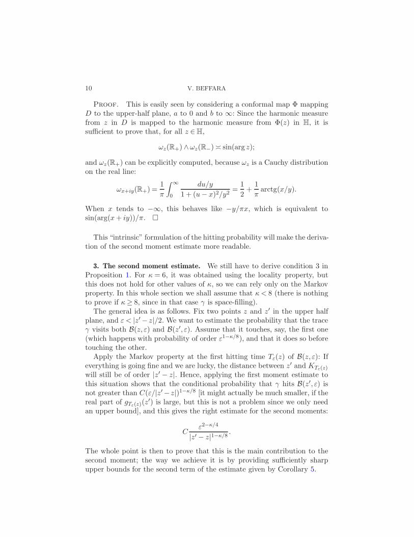
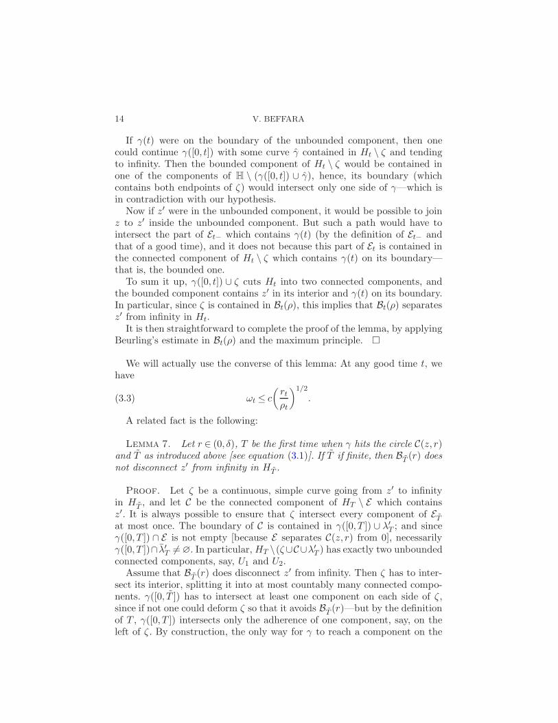
Fig. 1. Second moments: the setup.

3.1. Preliminaries. The first part of the proof is a succession of topologi-cal lemmas which allow for a precise estimation of the harmonic measures ofthe two sides of the SLE process. They are easier to state in the case κ≤ 4,for which the process consists in a simple curve. In the case 4< κ< 8, whathappens is that a positive area is “swallowed” by the process; in all the fol-lowing discussion, nothing changes as long as the points z and z′ themselvesare not swallowed, and the arguments are exactly the same—as all that isrequired for the proofs to apply is for the complement of the process to besimply connected and contain both z and z′.

On the other hand, if (say) z is swallowed at a given time, at which thecurve has not touched C(z, ε) yet, then this will never happen, so this eventdoes not contribute at all to the probability of the event we are interestedin. If the trace does touch C(z, ε) before swallowing z, then the swallowingoccurs at a time when it is not relevant anymore—since we know already thatz is ε-close to the path—so again the rest of the argument is not affected.

In order to simplify the exposition of the argument, we will implicitlyassume that indeed κ ≤ 4. The interested reader can easily check as sheproceeds that what follows does apply to the other cases, with little changein the writing.

Let z, z′ be two points in the upper half plane, and let δ = |z− z′|/2. Wecan assume that both ℑz and ℑz′ are greater than 18δ (say). Introduce a“separator set” (cf. Figure 1):

E = C(

z + z′

2,2δ

)

∪ w ∈H :d(w,z) = d(w,z′)≤ δ√

5.

At each positive time t, the complement Ht of Kt in H is an open andsimply connected domain, hence, its intersection with E is the disjoint unionof at most countably many connected sets, each separating Ht into two (orup to four for at most two of them) connected components. If both z and

12 V. BEFFARA

z′ are in Ht, let Et be the union of those crosscuts which disconnect z fromz′ in Ht; if either z or z′ is in Kt, let Et =∅—notice that in the case of anSLE process with parameter κ≤ 4, this almost surely never happens. Notethat, as long as z and z′ are in Ht, Et is not empty, because Ht is simplyconnected and E itself disconnects z from z′. The components of Et can thenbe ordered in the way they first appear on any path going from z to z′ inHt; let λt be the first one, and λ′t be the last one (which is also the first oneseen from z′ to z); for convenience, in the case Et =∅, let λt = λ′t =∅ too.

For each time t (possibly random), introduce

t := Infs > t :Ks ∩ λ′t 6=∅,(3.1)

t := Infs > t :Ks ∩ λt 6=∅,(3.2)

with the usual convention that the infimum of the empty set is infinite.Clearly, τ and τ are stopping times if τ is one.

Besides, Et does not change on any time-interval on which γ does notintersect E—hence, if for some t1 < t2, γ((t1, t2)) ∩ E = ∅, we can defineEt2− as its constant value on the interval (t1, t2) (i.e., as Et1). We say that apositive stopping time t is a good time if the following conditions are satisfiedwith probability 1:

• There exists s < t such that γ((s, t))∩ E =∅;• γ(t) ∈ Et−.

Examples of good times are t and t when t is a stopping time such thatγ(t) /∈ E holds with probability 1.

We first give two preliminary lemmas which will be useful in estimatingthe harmonic measures appearing in the statement of Corollary 5. They arenot specific to SLE, but they depend (as stated) on the fact that γ is asimple curve which does not contain z nor z′ (as is the case with probability1 in the case κ≤ 4); they have obvious counterparts obtained by exchangingz and z′ and replacing everywhere t with t.

For each positive time, let ωt (resp. ω′t) be the smaller of the harmonic

measures of the two sides of γ, from z (resp. z′) in Ht—this corresponds tothe term we want to estimate in the statement of Corollary 5. (Here andin all the sequel, as is natural, we include the positive real axis in the rightside of γ and the negative real axis in its left side.) Besides, for t > 0 andρ ∈ (0, δ), let Bt(ρ) [resp. B′

t(ρ)] be the closure of the connected componentof z (resp. z′) in B(z, ρ)∩Ht [resp. B(z′, ρ)∩Ht].

In all that follows we will use the following notation at each time t > 0(together with their counterparts around z′):

rt := d(z, γ([0, t]) ∪R);

ρt := Infρ ∈ (0, δ) :Bt(ρ) disconnects z′ from ∞ in Ht

THE DIMENSION OF THE SLE CURVES 13

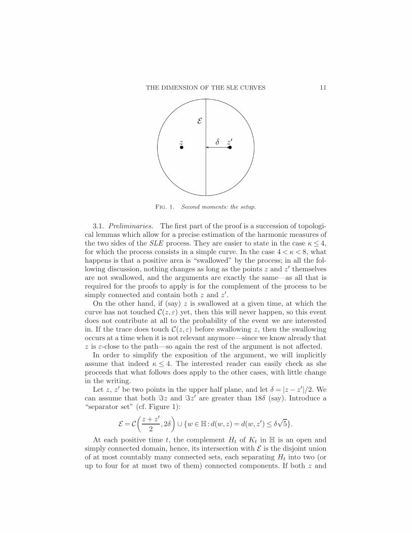
Fig. 2. Proof of Lemma 6.

(letting ρt = δ if the infimum is taken over an empty set). Obviously (rt)is nonincreasing; but (ρt) is not in general. Besides, ρt ≥ rt. Last, since thesets Bt(ρ) and γ([0, t]) are all compact, it is easy to see that at each time tsuch that ρt < δ, γ([0, t]) ∪Bt(ρt) itself does disconnect z′ from infinity.

Lemma 6. There exists a positive constant c such that the following hap-pens. Let t be a good time, and ρ ∈ (rt, δ). If ωt ≥ c(rt/ρ)

1/2, then γ([0, t]) ∪Bt(ρ) disconnects z′ from infinity; in particular, ρt ≤ ρ.

Proof. First make the following remark: For ρ ∈ (rt, δ), if the harmonicmeasure from z in Bt(ρ)\γ([0, t]) gives positive mass to both sides of γ, thenBt(ρ) separates z′ from infinity in Ht (see Figure 2).

Indeed, assume that we are this case. That means that there exist two dis-joint smooth curves ζ1, ζ2 : [0,1] →H satisfying ζ1(0) = ζ2(0) = z, ζi((0,1)) ⊂Bt(ρ) \γ([0, t]) and ζi(1) ∈ γ([0, t]), each landing on a different side of γ [i.e.,lims→1 gt(ζ1(s)) − βt ∈ (0,+∞) and lims→1 gt(ζ2(s)) − βt ∈ (−∞,0)—notethat such limits are always welldefined because gt extends continuously tothe boundary of Ht]. Let ζ = ζ1((0,1))∪ζ2((0,1))∪z be the correspondingcross-cut: The complement of ζ in Ht has exactly two (simply) connectedcomponents, one of which is unbounded.

14 V. BEFFARA

If γ(t) were on the boundary of the unbounded component, then onecould continue γ([0, t]) with some curve γ contained in Ht \ ζ and tendingto infinity. Then the bounded component of Ht \ ζ would be contained inone of the components of H \ (γ([0, t]) ∪ γ), hence, its boundary (whichcontains both endpoints of ζ) would intersect only one side of γ—which isin contradiction with our hypothesis.

Now if z′ were in the unbounded component, it would be possible to joinz to z′ inside the unbounded component. But such a path would have tointersect the part of Et− which contains γ(t) (by the definition of Et− andthat of a good time), and it does not because this part of Et is contained inthe connected component of Ht \ ζ which contains γ(t) on its boundary—that is, the bounded one.

To sum it up, γ([0, t]) ∪ ζ cuts Ht into two connected components, andthe bounded component contains z′ in its interior and γ(t) on its boundary.In particular, since ζ is contained in Bt(ρ), this implies that Bt(ρ) separatesz′ from infinity in Ht.

It is then straightforward to complete the proof of the lemma, by applyingBeurling’s estimate in Bt(ρ) and the maximum principle.

We will actually use the converse of this lemma: At any good time t, wehave

ωt ≤ c

(

rtρt

)1/2

.(3.3)

A related fact is the following:

Lemma 7. Let r ∈ (0, δ), T be the first time when γ hits the circle C(z, r)and T as introduced above [see equation (3.1)]. If T if finite, then BT (r) doesnot disconnect z′ from infinity in HT .

Proof. Let ζ be a continuous, simple curve going from z′ to infinityin HT , and let C be the connected component of HT \ E which containsz′. It is always possible to ensure that ζ intersect every component of ETat most once. The boundary of C is contained in γ([0, T ]) ∪ λ′T ; and sinceγ([0, T ]) ∩ E is not empty [because E separates C(z, r) from 0], necessarilyγ([0, T ])∩ λ′T 6=∅. In particular, HT \(ζ∪C∪λ′T ) has exactly two unboundedconnected components, say, U1 and U2.

Assume that BT (r) does disconnect z′ from infinity. Then ζ has to inter-sect its interior, splitting it into at most countably many connected compo-nents. γ([0, T ]) has to intersect at least one component on each side of ζ ,since if not one could deform ζ so that it avoids BT (r)—but by the definitionof T , γ([0, T ]) intersects only the adherence of one component, say, on theleft of ζ . By construction, the only way for γ to reach a component on the

THE DIMENSION OF THE SLE CURVES 15

other side of ζ is by intersecting C and hence λ′T , so it cannot happen before

time T .

In other words, if T is the first time when γ intersects C(z, r) and τ isthe first time t such that ρt ≤ r, then assuming that τ is finite, we haveT < T < τ .

The last lemma in this section is specific to SLE: It is a quantitativeversion of the transience of the curve γ and basically says that if γ formsa fjord, then it is not likely to enter it. With the modifications of notationdescribed later for the case 4 < κ < 8, it holds also in that case, and theproof is the same.

Lemma 8. Let γ be the trace of an SLE with parameter κ≤ 4; then thereexist positive constants C and η such that the following happens. Let ρ > 0and let τ be the first time t such that ρt ≤ ρ (i.e., such that γ([0, t]) ∪Bt(ρ)disconnects z′ from infinity). τ is finite with positive probability, in whichcase we have |γτ − z|= ρ, and:

1. P (τ <∞|Fτ , τ <∞)≤C(ρ/δ)η ;2. For every r < rτ ,

P (τ <∞, rτ < r|Fτ , τ <∞)≤C(r/rτ )1−κ/8(ρ/δ)η .

Proof. (i) In all this proof c will denote any finite positive constantwhich depends only on κ. Notice that if z′ ∈Kτ (which can happen if κ > 4),there is nothing to prove, since τ = ∞ in this case; so we assume from nowon that z′ /∈Kτ . Recall that λ′τ is the last component of Eτ that one has tocross when going from z to z′ in Hτ . By monotonicity, the extremal distancebetween E and Bτ (ρ) in Hτ is bounded below by 1

2π log(δ/ρ)—and hence sois the extremal distance between λ′τ and Bτ (ρ).

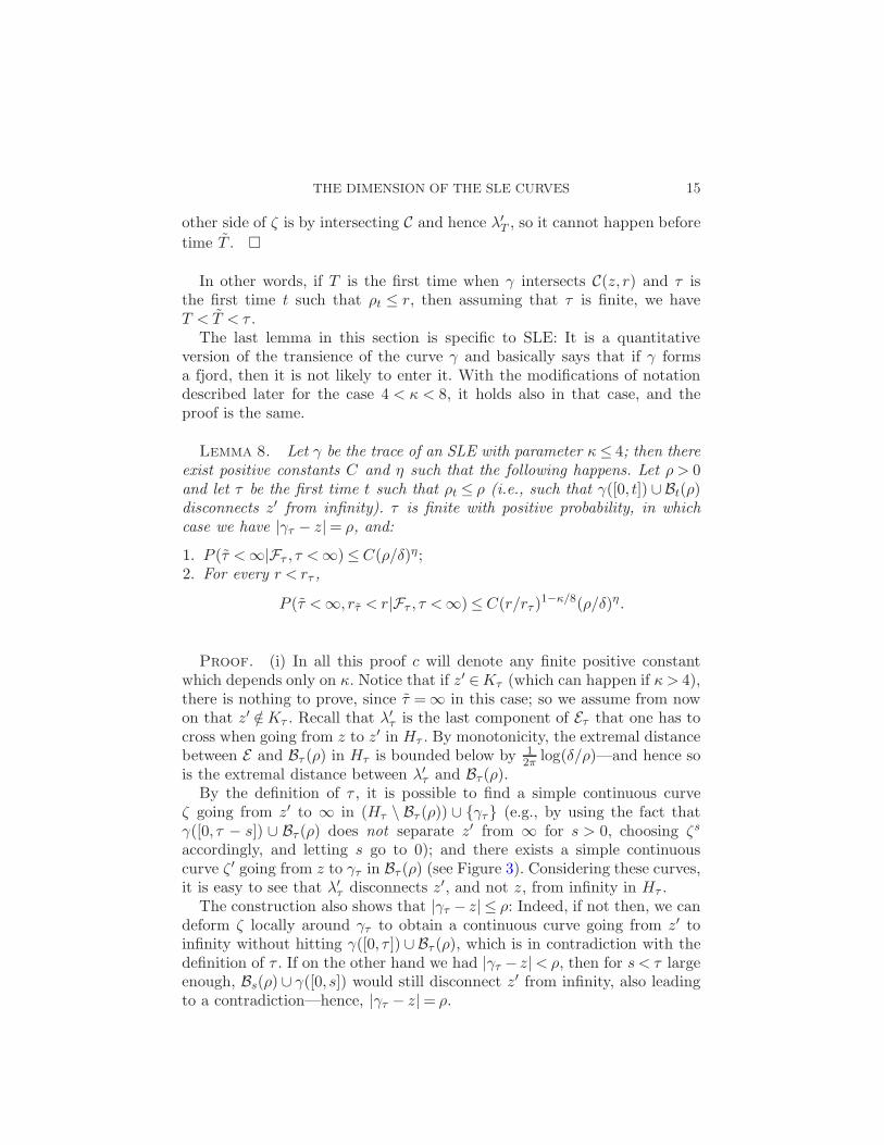
By the definition of τ , it is possible to find a simple continuous curveζ going from z′ to ∞ in (Hτ \ Bτ (ρ)) ∪ γτ (e.g., by using the fact thatγ([0, τ − s]) ∪ Bτ (ρ) does not separate z′ from ∞ for s > 0, choosing ζs

accordingly, and letting s go to 0); and there exists a simple continuouscurve ζ ′ going from z to γτ in Bτ (ρ) (see Figure 3). Considering these curves,it is easy to see that λ′τ disconnects z′, and not z, from infinity in Hτ .

The construction also shows that |γτ − z| ≤ ρ: Indeed, if not then, we candeform ζ locally around γτ to obtain a continuous curve going from z′ toinfinity without hitting γ([0, τ ]) ∪ Bτ (ρ), which is in contradiction with thedefinition of τ . If on the other hand we had |γτ − z|< ρ, then for s < τ largeenough, Bs(ρ) ∪ γ([0, s]) would still disconnect z′ from infinity, also leadingto a contradiction—hence, |γτ − z| = ρ.

16 V. BEFFARA

Fig. 3. Proof of Lemma 8: Setup.

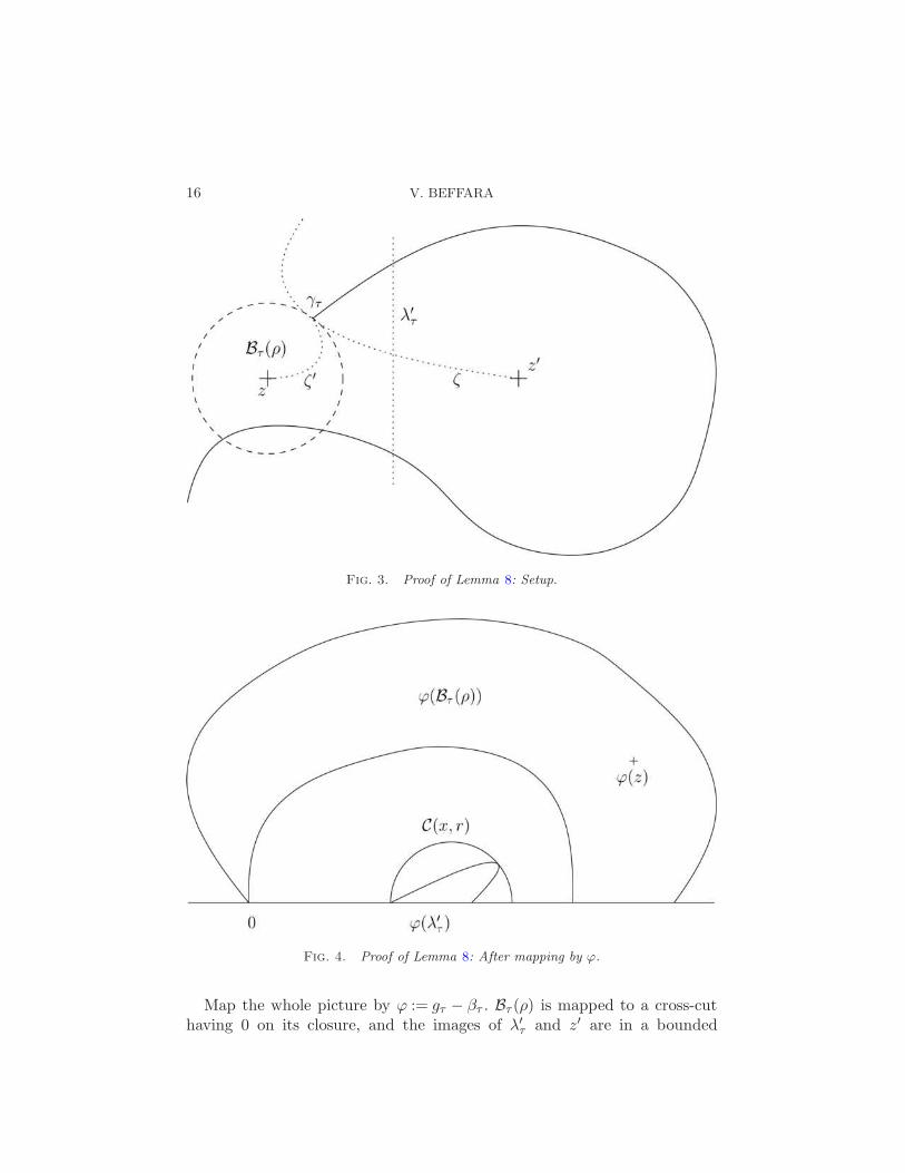
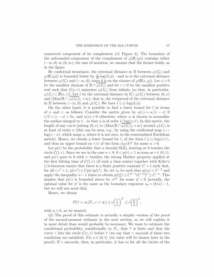
Fig. 4. Proof of Lemma 8: After mapping by ϕ.

Map the whole picture by ϕ := gτ − βτ . Bτ (ρ) is mapped to a cross-cuthaving 0 on its closure, and the images of λ′τ and z′ are in a bounded

THE DIMENSION OF THE SLE CURVES 17

connected component of its complement (cf. Figure 4). The boundary ofthe unbounded component of the complement of ϕ(Bτ (ρ)) contains either(−∞,0) or (0,∞); for ease of notation, we assume that the former holds, asin the figure.

By conformal invariance, the extremal distance in H between ϕ(λ′τ ) andϕ(Bτ (ρ)) is bounded below by 1

2π log(δ/ρ)—and so is the extremal distancebetween ϕ(λ′τ ) and (−∞,0), since 0 is on the closure of ϕ(B(z, ρ)). Let x > 0be the smallest element of R ∩ ϕ(λ′τ ) and let r > 0 be the smallest positivereal such that C(x, r) separates ϕ(λ′τ ) from infinity [so that, in particular,ϕ(λ′τ ) ⊂ B(x, r)]. Let l be the extremal distance in H \ϕ(λ′τ ) between (0, x)and (Max(R ∩ ϕ(λ′τ )),+∞), that is, the reciprocal of the extremal distancein H between (−∞,0) and ϕ(λ′τ ): We have l≤ c/ log(δ/ρ).

On the other hand, it is possible to find a lower bound for l in termsof x and r, as follows: Consider the metric given by u(z) = α/|z − x| ifr/5< |z − x|< 5x, and u(z) = 0 otherwise, where α is chosen to normalizethe surface integral to 1—so that α is of order 1/ log(x/r). In this metric, thelength of any curve joining (0, x) to (Max(R∩ϕ(λ′τ )),+∞) around ϕ(λ′τ ) isat least of order α [this can be seen, e.g., by using the conformal map z 7→log(z−x), which maps u, where it is not zero, to the renormalized Euclideanmetric]. Hence, we obtain a lower bound for l, of the form l ≥ c/ log(x/r),and thus an upper bound on r/x of the form c(ρ/δ)α for some α> 0.

Let p(r) be the probability that a chordal SLEκ starting at 0 touches thecircle C(1, r). Since we are in the case κ < 8, 0< p(r)< 1 as soon as r ∈ (0,1),and p(r) goes to 0 with r; besides, the strong Markov property applied atthe first hitting time of C(1, r) (if such a time exists) together with Kobe’s1/4-theorem ensure that there is a finite positive constant C > 1 such that,for all r, r′ < 1, p(rr′)≤Cp(r)p(r′). So, let r0 be such that p(r0)<C−2 andapply the inequality n− 1 times to obtain p(rn

0 ) ≤Cn−1(C−2)n ≤C−n. Thisimplies that p(r) is bounded above by crη′

for some η′ > 0 [actually, theoptimal value for η′ is the same as the boundary exponent sb = (8/κ) − 1,but we will not need this].

Hence, we obtain

P (τ <∞|Fτ , τ <∞) ≤ c

(

r

x

)η′

≤ c

(

ρ

δ

)η

,

with η > 0, as we wanted.(ii) The proof of this estimate is actually a simpler version of the proof

of the second-moment estimate in the next section, so we will explain itin more detail than would probably be necessary. We want to estimate theconditional probability, conditionally to Fτ , that τ is finite and that thecurve γ hits the circle C(z, r) before τ (we say that γ succeeds if these twoconditions are satisfied). Fix a ∈ (0,1) (its value will be chosen later in theproof): If γ succeeds, then, in particular, it has to hit all the circles of the

18 V. BEFFARA

form C(z, rτak) lying between γ(τ) and C(z, r), and (the relevant parts of)

all the circles of the form C(z, ρa−k) lying between γ(τ) and Eτ .The idea is then the following: For each possible ordering of these hitting

times, we will estimate the probability that the circles are hit in this par-ticular order, using the strong Markov property recursively together withprevious estimates; we can then sum over all possible orderings to obtain anestimate of the probability that γ succeeds.

For each k > 0, let Tk be the first hitting time of C(z, rτak) by γ. Besides,

let λk be the last connected component of C(z, ρa−k) ∩Hτ which a curvegoing from z to z′ has to cross, and let τk be the first hitting time of λk by γ.Last, let k1 (resp. k2) be the largest integer smaller than log(δ/ρ)/ log(1/a)[resp. log(rτ/r)/ log(1/a)]: It is sufficient to give an upper bound for theprobability that both τk1 and Tk2 are finite and smaller that τ .

We describe the ordering of the hitting times by specifying the successivenumbers of circles of each kind which γ hits before time τ . More precisely,assume that γ succeeds: Then there are nonnegative integers I , (mi)i≤I and(li)i≤I , all positive except possibly for m1 and lI , such that

τ1 < · · ·< τm1 < T1 < · · ·<Tl1 < τm1+1 < · · ·< τm1+m2 < · · ·<Tl1+···+lI < τ

and∑

mi = k1 and∑

li = k2 [so that γ first crosses m1 of the λk, then l1 ofthe C(z, rτa

k), then m2 new λk, etc.].Notice that at time τi, Beurling’s estimate in the domain B(z, rτ )\γ([0, τi])

shows that ωτiis at most equal to C(rτi

/rτ )1/2 (by Lemma 7 and the same

argument as the one used in the proof of Lemma 6). Besides, the same proofas that of point (i) in the present lemma shows the following: For givenvalues of the (mi) and (li), for each i, conditionally to FTl1+···+li

and thefacts that Tl1+···+li <∞ and that the last τ -time happening before Tl1+···+li

is τm1+···+mi(as will be the case in the construction), P (τm1+···+mi+1 <

∞|FTl1+···+li) is bounded by Caηmi+1 .

For given values of I and the (mi) and (li), applying the strong Markovproperty at each of the times Tl1+···+li and τm1+···+mi

, we get an estimate ofthe conditional probability (conditionally to Fτ ) that γ succeeds with thisparticular ordering, as a product of conditional probabilities, namely,

I∏

i=1

P (τm1+···+mi<∞|FTl1+···+li−1

)P (Tl1+···+li <∞|Fτm1+···+mi).

Using the previous estimates, and Corollary 5, this product is bounded aboveby

I∏

i=1

Caηmi(al1+···+li−1)(8/κ−1)/2(ali)1−κ/8.

THE DIMENSION OF THE SLE CURVES 19

It remains to sum this estimate over all possible values of I , the mi andthe li. We get the following, where as is usual C is allowed to change fromline to line, but depends only on κ and later on a:

P (τk1 < τ,Tk2 < τ) ≤∞∑

I=1

∑

(mi),(li)

I∏

i=1

Caηmi(al1+···+li−1)(8/κ−1)/2(ali)1−κ/8

≤ aηk1+(1−κ/8)k2

∞∑

I=1

CI∑

(mi),(li)

I∏

i=1

(al1+···+li−1)(8/κ−1)/2

= aηk1+(1−κ/8)k2

∞∑

I=1

CI∑

(mi),(li)

I∏

i=1

(a(I−i)li)(8/κ−1)/2.

For a fixed value of I , the number of possible choices for the mi (which areI integers of sum k1) is smaller than 2I+k1 , hence, replacing C by 2C, weget

P (τk1 < τ,Tk2 < τ)≤ aηk1+(1−κ/8)k22k1

∞∑

I=1

CI∑

(li)

I∏

i=1

(a(I−i)li)(8/κ−1)/2.

The sum over (li) is taken over all I-tuples of positive integers with sumk2, so if the first I − 1 are known, so is the last one. An upper bound isthen given by relaxing the condition l1 + · · ·+ lI = k2 and simply summingover all positive values of l1, . . . , lI−1 (lI does not contribute to the productanyway). So we obtain

P (τk1 < τ,Tk2 < τ)≤ aηk1+(1−κ/8)k22k1

∞∑

I=1

CII−1∏

i=1

∑

l>0

(a(I−i)l)(8/κ−1)/2.

We can sum over l > 0 in each term of the product; each sum will be equal toa(I−i)(8/κ−1)/2 up to a constant which, if a is chosen small enough, is smallerthan 2. Hence, a factor 2I which can again be made part of CI by doublingthe value of C:

P (τk1 < τ,Tk2 < τ)≤ aηk1+(1−κ/8)k22k1

∞∑

I=1

CII−1∏

i=1

(a(I−i))(8/κ−1)/2.

Compute the product explicitly: The exponent of a is then the sum of theI − i for 1 ≤ i≤ I − 1, which is equal to I(I − 1)/2. The linear term −I/2can be incorporated in the factor CI (making C depend on a now, whichwill not be a problem), leading to

P (τk1 < τ,Tk2 < τ) ≤ aηk1+(1−κ/8)k22k1

∞∑

I=1

CI(aI2/2)(8/κ−1)/2

20 V. BEFFARA

≤ (2aη/2)k1a(η/2)k1+(1−κ/8)k2

∞∑

I=1

CI(aI2/2)(8/κ−1)/2.

Now pick a small enough that 2aη/2 is smaller than 1. The sum in theprevious expression is finite (because κ < 8 and a < 1), so we obtain

P (τk1 < τ,Tk2 < τ) ≤Ca(η/2)k1+(1−κ/8)k2 ,

which implies the announced result.

Remark 1. It is possible to simplify the statement of the last part ofthe proof of the lemma (though unfortunately not the computation) in thefollowing way. Let m = (mi) and l = (li) be the jump sizes of the process,which we will interpret as ordered partitions of k1 and k2, respectively. Asis customary, we write this as m ⊢ k1, respectively l ⊢ k2. The length of thepartitions, that is, I , will be denoted as |m| = |l|. Let l+ be the cumulativesum of l, that is, the sequence (l1 + · · ·+ li)1≤i≤I−1. Using am as a shortcutfor the product of the ami , the main step in the proof of (ii) above is thefollowing inequality, valid for any positive exponents α, β and γ and for asmall enough that 4caγ/2 < 1: Uniformly in k1 and k2,

∑

m⊢k1,l⊢k2,|l|=|m|

aαm+βl+γl+c|l| ≤Caαk1/2+βk2 .(3.4)

The direct use of this inequality and similar notation will greatly simplifythe writing of the proof in the next section.

Remark 2. One could describe the behavior of the system in the proofof point (ii) in a different way. Let mt (resp. lt) be the value of k correspond-ing to the last λk [resp. C(z, rτa

k)] discovered by γ by time t (or 0 if t < τ1,resp. t < T1). The process (mt, lt) takes values in N2; looking at it at timesTl1+···+li , one can couple it with a discrete-time Markov chain (Mi,Li) inΩ =N2 ∪ ∆, with an absorbing state ∆ and transition probabilities givenby the following:

• P (Mi+1 =Mi +m,Li+1 =Li + l|Mi,Li) = 0 if m≤ 0 or l≤ 0,• P (Mi+1 = Mi + m,Li+1 = Li + l|Mi,Li) ≤ Caηm+(8/κ−1)Mi/2+(1−κ/8)l ifm> 0 and l > 0.

The probability estimate provided by point (ii) of the previous lemma isthen bounded above by the probability that this Markov chain, started at(0,0), reaches the domain Dk1,k2 = Jk1,∞J×Jk2,∞J. Such a probability canbe estimated by summing the probabilities of all possible paths going from(0,0) to Uk1,k2 (which corresponds to the proof we just gave), or by findingan appropriate super-harmonic function on N2. However, we could not finda simple expression for such a super-harmonic function.

THE DIMENSION OF THE SLE CURVES 21

3.2. The proof. Applying Lemma 6, Corollary 5 and the strong Markovproperty, we obtain the following estimate (which we will refer to as themain estimate): For every good time t and every radius r ∈ (0, rt),

P (γ([t,∞)) ∩B(z, r) 6=∅|Ft, t <∞)≤C

(

r

rt

)s( rtρt

)sb/2

,(3.5)

where we define the hull and boundary exponents by

s= 1− κ

8and sb =

8

κ− 1

and where C depends only on κ. The way to obtain the required second-moment estimate from this upper bound is actually quite similar in spirit tothe way we proved point (ii) of Lemma 8: We will split the event that γ hitstwo small disks according to the order in which it visits a finite family ofcircles, estimate each of these individual probabilities as a product using thestrong Markov property, and then sum over all possibilities. The notation isquite heavier than previously, though.

Introduce a small constant a ∈ (0,1) (the value of which will be deter-mined later) and let δn = anδ. We will split the event

Eε(z, z′) := B(z, ε) ∩ γ([0,∞)) 6=∅,B(z′, ε) ∩ γ([0,∞)) 6=∅

according to the order in which the processes (rt), (r′t), (ρt) and (ρ′t) reachthe values δn. For convenience, let n = ⌊log(ε/δ)/ log a⌋: It is sufficient toestimate the probability that both (rt) and (r′t) reach the value δn.

Let Tn (resp. T ′n, τn, τ ′n) be the first time when rt (resp. r′t, ρt, ρ

′t) is not

greater than δn (or infinity, if such a time does not exist). We will call allthese stopping times discovery times.

Lemma 9. For all n,n′ > 0, we have the following (as well as their coun-terparts obtained by exchanging the roles of z and z′) if all the involvedstopping times are finite:

1. γτn ∈ C(z, δn)∩Bτn(δn); in particular, |γτn − z| = δn;2. Tn < Tn+1 and τn < τn+1;3. Tn < τn;4. If Tn < T ′

n′ , then Tn < T ′n′ , and similarly replacing T (resp. T ′, resp. both)

by τ (resp. τ ′, resp. both).

Proof. Point (i) was proved as part of Lemma 8; point (ii) is thenobvious and point (iii) is a direct consequence of Lemma 7, so only (iv)requires a proof.

Assume that Tn < T ′n′ . Let ζ be a curve going from z to z′, obtained

by concatenating ζ1 ⊂BTn(δn), γ([Tn, T′n′ ]) and ζ2 ⊂BT ′

n′(δn′). Such a curve

22 V. BEFFARA

has to cross λ′Tn(by definition), and that can only happen on γ((Tn, T

′n′))

because the distance between ETn and z (resp. z′) is greater than δn (resp.δn′). This is equivalent to saying that Tn < T ′

n′ , which is what we wanted.The same reasoning applies when replacing T by τ and/or T ′ by τ ′.

Here is a somewhat informal description of the construction we will do.Assume that γ hits both B(z, δn) and B(z′, δn). In order to do it, it has tocross all the circles of radii δn, n≤ n around z and z′, and it will do so ina certain order, coming back to the separator set E between explorationsaround z and around z′ [this is the meaning of point (iv) of the previouslemma]. We call a task the time interval spanning between two successivesuch returns on E . The conditional probability that a given task is performed,conditionally to its past, is then given by the main estimate (3.5), and therest of the construction is then very similar to the proof of point (ii) inLemma 8.

Let S0 = 0 and define the stopping times Si and S′i for i > 0, inductively,

as follows:

• S′i = Min(Tn, T

′n, τn, τ

′n∩ (Si−1,∞)), that is, S′

i is the first discovery timeafter Si−1, if such a time exists;

• Si = S′i if S′

i is a Tn or a τn, Si = S′i if S′

i is a T ′n or a τ ′n—again if such a

time exists.

Continue the construction until the first ball of radius δn is hit by thecurve; let I be chosen in such a way that this happens at time S′

I−1. Thecurve still has to come back to E after that, so SI−1 is well defined. Then,simply let SI be the hitting time of the second ball of radius δn. We calltask a time-interval of the form (Si−1, Si]; I is then simply the number oftasks. Following our construction, the last task is different from the othersand will have to be treated specially.

For each i≤ I , let Ji (resp. Ki, J′i , K

′i) be the largest integer n > 0 for

which τn (resp. Tn, τ ′n, T ′n) is smaller than Si, if such an integer exists, and

0 if it does not. By construction,

δKi+1 < rSi≤ δKi

, δJi+1 < ρSi,

and similar inequalities hold for r′Siand ρ′Si

.So, we obtain a sequence of quadruples (Ji,Ki, J

′i ,K

′i)i≤I , which is not

Markovian but on which we can say enough to obtain the needed second-moment estimate. First of all, for each i < I , at least one of Ji+1, Ki+1, J

′i+1,

K ′i+1 is larger than its counterpart at index i; but if Ji+1 > Ji or Ki+1 >Ki,

then J ′i+1 = J ′

i and K ′i+1 =K ′

i, by point (iv) of Lemma 9. The main estimateimplies the following bound: for each k > 0,

P ((Ji+1,Ki+1, J′i+1,K

′i+1) = (Ji,Ki + k,J ′

i ,K′i)|FSi

)(3.6)

≤Casb(Ki−Ji)/2ask.

THE DIMENSION OF THE SLE CURVES 23

Point (ii) of Lemma 8 then says that, for every j > 0 and k ≥ 0, and ifi < I − 1,

P ((Ji+1,Ki+1, J′i+1,K

′i+1) = (Ji + j,Ki + k,J ′

i ,K′i)|FSi

)(3.7)

≤Caη(Ji+j)ask.

The first of these bounds also applies in the second case, still as a conse-quence of the main estimate, so we get a last estimate for the last step: forevery j > 0,

P ((JI ,KI , J′I ,K

′I) = (JI−1 + j, n, J ′

I−1, n)|FSI−1)

(3.8)≤Casb(KI−1−JI−1)/2ask.

Notice that here and from now on, as the estimates on radii we get fromthe values of the J and K are only valid up to a multiplicative factor of ordera, the constants C appearing in the estimates now depend on the value ofa.

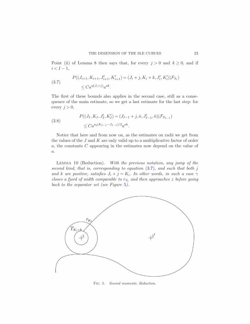
Lemma 10 (Reduction). With the previous notation, any jump of thesecond kind, that is, corresponding to equation (3.7), and such that both jand k are positive, satisfies Ji + j =Ki. In other words, in such a case γcloses a fjord of width comparable to rSi

and then approaches z before goingback to the separator set (see Figure 5).

Fig. 5. Second moments: Reduction.

24 V. BEFFARA

Proof. First notice that Lemma 7 ensures that Ji +j ≤Ki; assume thatJi + j <Ki. Let τ = τJi+j and T = TKi+k, and assume that both lie betweenSi and Si+1 and that τ < T : At time τ , the situation is similar to the onein Lemma 8. Construct ζ ′ as in the proof of Lemma 8, and continue ζ ′ to acrosscut ζ ′ separating z′ from infinity, and still contained in Bτ (δJi+j)—thisis possible by the definition of τ . Let τ ′ be the first time after τ such thatγτ ′ ∈ ∂Bτ (δKi

) (necessarily τ ′ <T ). Let ζ ′′ be a continuous curve joining γτ ′

to z inside Bτ (δKi). Because the unbounded component of Hτ \λ′τ is simply

connected, the concatenation of ζ ′′ and γ([τ ′, τ ]) is homotopic to ζ ′, and inparticular, it separates λ′τ from infinity. Hence, Bτ (δKi

) separates z′ frominfinity in Hτ ′ , and in particular, τKi

< T . This contradicts the hypothesisJi + j <Ki.

The same construction applies if, among the discovery times lying betweenSi and Si+1, there is a τ -time before a T -time. The last case to consider isthen when T = TKi+k happens before any closing time. In particular, if suchis the case, BT (δJi+1) does not separate z′ from infinity in HT . The sameproof as that of Lemma 7 then shows that τJi+1 > T = Si+1, which again isa contradiction.

This reduction means that, as far as reaching probabilities are concerned,the jump from (Ji,Ki) to (Ji + j,Ki + k) behaves exactly like the successionof two jumps, from (Ji,Ki) to (Ji + j,Ki) = (Ki,Ki) (which happens withprobability not greater than Caη(Ji+j)) and then from (Ki,Ki) to (Ki,Ki +k) (which happens with probability not greater than Cask): Up to replacingC with C2, we can assume in the computations that jumps of the typecorresponding to equation (3.7) only happen with k = 0, and

P ((Ji+1,Ki+1, J′i+1,K

′i+1) = (Ji + j,Ki, J

′i ,K

′i)|FSi

)≤Caη(Ji+j).(3.9)

Again, this estimate does not hold for the very last task—which, accordingto this decomposition, would correspond to the fact that the last two jumpsare a jump of J followed by a jump ofK, this last one reaching the value n. Inthat case, with the notation in equation (3.8), we would have j =KI−1−JI−1

from the previous Lemma. Assuming that η < sb/2, which we can do, we thenobtain the following estimate for the second-to-last jump in the previousreduction (the last jump always involves K):

P ((JI−1,KI−1, J′I−1,K

′I−1) = (JI−2 + j,KI−2, J

′I−2, n)|FSI−2

)(3.10)

≤Caηj .

In other words, here only the last jump of J appears in the exponent asopposed to the end-value in the other cases. (In fact, using the main estimatehere amounts to discarding that last jump of J entirely, but writing the

THE DIMENSION OF THE SLE CURVES 25

estimate this way makes for a slightly more pleasant computation below.)This turns out to be enough for our purposes.

All we need to do then is to estimate the probability that (Ki,K′i) reaches

(n, n). With this formulation, it would be nice to give a super-harmonic func-tion associated to the process, but despite our best effort, we could not findsuch a function. The natural candidate would be of the form C ′as(n−K)+η(K−J)/2,but this might fail to be super-harmonic along the diagonal—the reason be-ing that C now depends on a.

So, we will apply the same strategy as in the proof of point (ii) of Lemma 8,namely, sum over all possible paths starting at (0,0,0,0) and ending on(J, n, J ′, n) for some J,J ′ ∈ J0, nK (which we will call good paths). This leadsto rather unpleasant computations, but the general strategy should be clearenough.

Look first at the components Ji and Ki of the walk: Along a good path,the jumps of (Ji,Ki) affect either its first or its second coordinate. Let n≥ 0be the number of jumps affecting (Ji), and let j1, . . . , jn > 0 be their lengths.Then, for 0 ≤ i≤ n, let li ≥ 0 be the number of jumps affecting K betweenthe ith and (i+ 1)st jumps of J , and let ki,1, . . . , ki,li > 0 be their lengths—with the obvious abuse of notation that l0 is the number of jumps of Kbefore the first jump of J , and ln is the number of jumps of K after the lastjump of J . In particular, the sum of all ki,j is equal to n. Define the integersn′, j′i, l

′i and k′i,j in a similar fashion to describe the behavior of (J ′

i ,K′i).

Notice that, just before the jump corresponding to ji, the value of J isj1 + · · ·+ ji−1. Besides, let di ≥ 0 be the value of K− J just after that jump(di is the difference between the sum of the k’s and that of the j’s so far):Just before the jump corresponding to ki,j , the value of K − J is equal todi + ki,1 + · · · + ki,j−1. This is sufficient to estimate the probability that agiven path occurs: It will be given by the product along the path of the(conditional, given the past) probabilities of the individual steps, which isbounded above by the product of two terms, namely,

A := a−η(j1+···+jn−1)

×l0∏

j=1

C(ak0,j )s(ak0,1+···+k0,j−1)sb/2

×n∏

i=1

[

C(aj1+···+ji)ηli∏

j=1

C(aki,j)s(adi+ki,1+···+ki,j−1)sb/2

]

.

Here, the empty products are equal to 1 by convention. The term a−η(j1+···+jn−1)

accounts for the difference in the very last task, where as was pointed outabove, only the last jump of J , that is, jn, appears in the exponent. Thattask might be a jump toward z′, or not involve a jump of J at all, in which

26 V. BEFFARA

case the factor would not be needed, but having it in all cases makes thecomputation more symmetric—it not smaller than 1 anyway.

Also define the corresponding A′ involving n′, j′i, l′i and k′i,j . With the

shortcut notation used in the previous subsection, letting j = (ji) and ki =(ki,j), so that |j| = n and |ki|= li, this becomes

A= a−ηj+n−1C |j|+

∑

|ki|ask0asbk+0 /2aηj+

n∏

i=1

[askiasbk+i

/2a|ki|disb/2].

Rewriting the product using the fact that∑

ki,j = n, and letting j0 =d0 = 0 for ease of notation, we obtain

A= a−ηj+n−1Cn+∑

liasnl0∏

j=1

(ak0,1+···+k0,j−1)sb/2

×n∏

i=1

[

(aj1+···+ji)ηli∏

j=1

(adi+ki,1+···+ki,j−1)sb/2

]

= a−ηj+n−1Cn+

∑

liasnn∏

i=0

[

(aj1+···+ji)ηli∏

j=1

(adi+ki,1+···+ki,j−1)sb/2

]

= Cn+∑

liasnaηjn

n∏

i=0

[

a(n−i)ηji+lidisb/2li−1∏

j=1

a(li−j)ki,jsb/2

]

.

Indeed, each term aji for i < n appears n− i times in the product, the termajn appears once [in other terms, aji appears (n− i)∨ 1 times], the term adi

appears li times and the term aki,j appears li − j times.We still have to sum the product AA′ over all the good paths. Notice first

that giving the values of n, ji, li and ki,j , n′, j′i, l

′i and k′i,j is not sufficient

to specify the path of (J,K,J ′,K ′), because it says nothing about the waythe jumps of (J,K) and (J ′,K ′) are intertwined; however, there are at most

(

n+∑

li + n′ +∑

l′in+

∑

li

)

≤ 2n+∑

li2n′+∑

l′i

such intertwinings. Hence, up to doubling of the constant C, it is sufficientto sum AA′ over the values of n, ji, li and ki,j , n

′, j′i, l′i and k′i,j . The sum

will factor into two terms, one involving the terms around z and the otherthe terms around z′, and these two factors are equal. Hence, an upper boundof the probability that (K,K ′) reaches (n, n) is given by B2, where

B :=∑

j,ki

a−ηj+n−1C |j|+∑

|ki|ask0asbk+0 /2aηj+

n∏

i=1

[askiasbk+i

/2a|ki|disb/2],

with a sum taken over all values of the indices leading to a good path.

THE DIMENSION OF THE SLE CURVES 27

First, let ki =∑lj

j=1 ki,j (and notice that di = di−1 + ki−1 − ji). We can

rewrite B2 as

B2 = a2sn

[

∞∑

n=0

Cnn∏

i=0

[

∑

ji,ki

a[(n−i)∨1]ηji∑

li,ki,j

C lialidisb/2li−1∏

j=1

a(li−j)ki,jsb/2

]]2

,

where the innermost sum is taken over all choices of li and ki,j satisfying∑

ki,j = ki, and where the sum over ji is in fact not present for i= 0. This inturn can be considered as a sum over the ki,j for j ≤ li − 1 with sum smallerthan ki. The case ki = li = 0 needs to be treated separately here, and we get

B2 ≤ a2sn

[

∞∑

n=0

Cnn∏

i=0

[

∑

ji

a[(n−i)∨1]ηji

(

1 +∑

ki,li>0

C lialidisb/2

×li−1∏

j=1

(

∑

k>0

a(li−j)ksb/2

))]]2

.

The sum over k can be computed explicitly, it is convergent because j <li and its value is smaller than 2a(li−j)sb/2 if a is chosen small enough,which we will assume from now on. The product over j is then equal to2li−1ali(li−1)sb/4. The terms with an exponent linear in li can be factoredinto C li—note that C now depends on a—leading to

B2 ≤ a2sn

[

∞∑

n=0

Cnn∏

i=0

[

∑

ji

a[(n−i)∨1]ηji

(

1 +∑

di,li

C lialidisb/2al2isb/4

)]]2

≤ a2sn

[

∞∑

n=0

Cnn∏

i=0

[

∑

ji

a[(n−i)∨1]ηji

(

1 +∑

di≥0

adisb/2∑

li>0

C lial2isb/4

)]]2

.

The sums over li and di are convergent, because a < 1, so the whole termin parentheses is bounded by a constant depending only on κ and a; sinceit appears n+ 1 times, up to another change in the value of C, we get

B2 ≤ a2sn

[

∞∑

n=0

Cn+1n∏

i=1

[

∑

ji>0

a[(n−i)∨1]ηji

]]2

.

Summing over all values of ji > 0, we obtain (if a is small enough)

B2 ≤ a2sn

[

∞∑

n=0

Cn+12aηn−1∏

i=1

(2a(n−i)η)

]2

.

Up to yet another increase of C, the factor 2 can be made part of it, andthe product over i can be computed explicitly:

B2 ≤ a2sn

[

∞∑

n=0

Cn+1aηan(n−1)η/2

]2

.

28 V. BEFFARA

This last sum is again convergent, so we obtain B2 ≤Ca2sn, with a constantC depending only on κ and a.

Putting everything together, assuming Eε(z, z′) holds, first γ has to reach

E , and this happens with probability of order δs. Then, conditionally tothe process up to this hitting time, we can apply the previous reasoningwhich says that the conditional probability to hit both disks of radius δn isbounded above by Ca2ns where C depends only on a and κ. Hence,

P (Eε(z, z′))≤Cδsa2ns.

Notice that an ≤ (ε/δ)a−1 to finally obtain

P (Eε(z, z′))≤Ca−2s ε

2s

δs,

which is precisely the estimate we were looking for.

4. The occupation density measure. As a side remark, let us consider theproof of the lower bound for the dimension (cf. Section 1). It is based on theconstruction of a Frostman measure µ supported on the path, constructedas a subsequential limit of the family (µε) defined by their densities withrespect to the Lebesgue measure on the upper-half plane:

dµε(z) = ε−s1z∈Cε |dz|.Then, µ is a random measure with correlations between µ(A) and µ(B), fordisjoint compact sets A and B, decaying as a power of their inverse distance.So, at least formally, it behaves in this respect like a conformal field: the one-point function (corresponding to the density of µ) is not welldefined, becauseµ is singular to the Lebesgue measure, but the two-point correlation

limδ→0

δ−4 Cov(µ(B(z, δ)), µ(B(z′, δ)))

behaves like d(z, z′)−1+κ/8.A little more can be said about this measure, or about its expectation. The

proof of the estimate for P (γ ∩ B(z, ε) 6=∅) can be refined in the followingway: When we apply the stopping theorem (2.8), saying that the diffusionconditioned to survive has a limiting distribution shows that

E

[

sin

(

αs

2

)8/κ−1∣∣

∣S ≥ s

]

has a limit λ when s→∞, and that this limit depends only on κ. So whatwe get out of the construction in Section 2 is

P

(

∃t > 0 : |g′t(z)| ≥ℑ(z)

ε

)

∼ε→0

λ(κ)

(

ε

ℑz

)1−κ/8

(sin(arg(z)))8/κ−1.

THE DIMENSION OF THE SLE CURVES 29

This lead us to an estimate on P (d(z, γ)< ε) by the Kobe 1/4 theorem; butit is also natural to measure the distance to γ by the modulus of g′. We cannow define

φ1(z) = limε→0

εκ/8−1P

(

∃t > 0 : |g′t(z)| ≥ℑ(z)

ε

)

:

the previous estimate boils down to

φ1(z) = λ(κ)ℑ(z)κ/8−1 sin(arg z)8/κ−1,

and by the construction of µ, we obtain that, for every Borel subset A ofthe upper-half plane,

E(µ(A)) ≍∫

Aφ1(z)|dz|,

with universal constants.It is then possible to do this construction for several points; note first that

the second moment estimate can actually be written as

P (z, z′ ⊂Cε)≍ε2(1−κ/8)

|z − z′|1−κ/8ℑ((z + z′)/2)1−κ/8,

as long as both ℑ(z) and ℑ(z′) are bounded below by |z − z′|/M for somefixed M > 0. Indeed, the upper bound is exactly what we derived in theprevious section, and the lower bound is provided by the term n= n′ = 0 inthe sum. Hence, any subsequential limit ψ(z, z′), as ε vanishes, of

ε2(κ/8−1)P (z, z′ ⊂Cε)

satisfies ψ(z, z′) ≍ φ2(z, z′) for some fixed function φ2, with constants de-

pending only on κ. The second moment estimate then shows that

φ2(z, z′) ≍

z′→z

φ1(z)

|z − z′|1−κ/8,

that is, φ2 behaves like a correlation function when z and z′ are close toeach other.

The general case of n points, n≥ 2, can be treated in the same fashion.First, the derivation of second moments admits a generalization to n points,as follows. Let (zi)1≤i≤n be n distinct points in H, such that their imaginaryparts are large enough (bigger than, say, 18n times the maximal distancebetween any two of them). We use them to construct a Voronoi tessellationof the plane; denote by Ci the face containing zi, and by δi the (Euclidean)distance between zi and ∂Ci. Let C(z0, δ0) be the smallest circle containingall the discs B(zi, δi). Last, let E be the “separator set” between the zi’s,defined as

E = C(z0, δ0)∪[(

n⋃

i=1

∂Ci

)

∩B(z0, δ0)

]

.

30 V. BEFFARA

It is the same as defined previously in the case n= 2.The previous proof can then be adapted to show that

P (z1, . . . , zn ⊂Cε) ≍(

δ0εn

∏

δi

)1−κ/8

(using radii δiak for the circles around zi). In the case n= 2, we have δ1 =

δ2 = δ0/2, so this estimate is exactly the same as previously. So, it makessense to take a (subsequential) limit, as ε tends to 0, of

εn(κ/8−1)P (z1, . . . , zn ⊂Cε),

and all possible subsequential limits are comparable to a fixed symmetricfunction φn.

The behavior of φn(z1, . . . , zn) when zn approaches the boundary is thengiven by the boundary term in Proposition 4, that is, φ behaves like (ℑzn)8/κ−1

there. Last, it is easy to see that, when zn tends to z1, φn(z1, . . . , zn) has asingularity which is comparable to |zn − z1|κ/8−1; in other words, we have arecursive relation between all the φn’s, given by

φn(z1, . . . , zn) ≍zn→z1

φn−1(z1, . . . , zn−1)

|zn − z1|1−κ/8,(4.1)

φn(z1, . . . , zn) ≍ℑzn→0

φn−1(z1, . . . , zn−1) · (ℑzn)8/κ−1.(4.2)

These relations are very similar to some of those satisfied by the corre-lation functions in conformal field theory. In fact, it is possible to push therelation further, in two ways. First, we can look at the evolution of the sys-tem in time. This corresponds to mapping the whole picture by the mapgt − βt, and this map acts on the discs of small radius around the zi’s likea multiplication of factor |g′t(zi)| (as long as Kt remains far away from thezi’s, which we may assume if t is small enough). Hence, the process

Y nt :=

(

∏

|g′t(zi)|1−κ/8)

φn(gt(z1)− βt, . . . , gt(zn)− βt)

(defined as long as all the zi’s remain outside Kt) is a local martingale. Wecan apply Ito’s formula to compute dY n

t , and write that the drift term hasto be 0 at time 0 to obtain a PDE satisfied by φn.

Note though that the formula involves the modulus of g′t, meaning thatthe equation we would obtain cannot be expressed in terms of complexderivatives of gt only, and that we have to introduce derivatives with respectto the coordinates. This is also the case for the second-order term in Ito’sformula: Since β is a real process, we would obtain terms involving secondderivatives of φn with respect to the x-coordinates of the arguments. To sumit up, it would be an ugly formula without the correct formalism—which is

THE DIMENSION OF THE SLE CURVES 31

why we do not put it here. The formula is much nicer when consideringpoints on the boundary of the domain—compare [5].

The last thing we can do is study what happens if we add one pointzn+1 to the picture. This will add one multiplicative factor, corresponding(at least intuitively) to the conditional probability to hit zn+1 knowing thatwe touch the first n points already. In the case κ = 8/3 and for points onthe boundary of the domain, this can be computed using the restrictionproperty, and it leads to Ward’s equations (cf. [5]). In the “bulk” (i.e., forpoints inside the domain), or for other values of κ, it is not clear yet how todo it.

5. The boundary. A natural question is the determination of the di-mension of the boundary of Kt for some fixed t, in the case κ > 4. Theconjectured value is

dimH(∂Kt) = 1 +2

κ,

and this can now be proved for a few values of κ for which the boundaryof K can be related to the path of an SLEκ′ with κ′ = 16/κ. In fact, thisrelation is only known in the cases where convergence of a discrete model toSLE is known, namely:

• κ = 6, where actually both ∂Kt and the path of the SLEκ′ are closelyrelated to the Brownian frontier. Hence, we obtain a third derivation ofthe dimension of the Brownian frontier, this time through SLE8/3.

• κ= 8: Here, SLE8 is known to be the scaling limit of the uniform Peanocurve and SLE2 that of the loop-erased random walk (cf. [12]). Since thesetwo discrete objects are closely related through Wilson’s algorithm, thisshows that the local structure of the SLE2 curve and the SLE8 boundaryare the same, and in particular, they have the same dimension.

So we obtain one additional result here:

Corollary 11. Let (Kt) be a chordal SLE8 in the upper-half plane:Then, for all t > 0, the boundary of Kt almost surely has Hausdorff dimen-sion 5/4.

It would be nice to have a direct derivation of the general result, withoutusing the “duality” between SLEκ and SLE16/κ; but it is not even clear howto obtain a precise estimate of the probability that a given ball intersectsthe boundary of K1.

32 V. BEFFARA

Acknowledgments. Part of this work was carried out during my stay atthe Mittag–Leffler institute whose hospitality and support is acknowledged.I also thank Peter Jones, Greg Lawler and Wendelin Werner for very usefuldiscussions, and I especially wish to thank Oded Schramm for his help andpatience in reviewing several draft versions of this paper.

REFERENCES

[1] Bass, R. F. (1998). Diffusions and Elliptic Operators. Springer, New York.MR1483890

[2] Beffara, V. (2004). Hausdorff dimensions for SLE6. Ann. Probab. 32 2606–2629.MR2078552

[3] Camia, F. and Newman, C. M. (2006). The full scaling limit of two-dimensional

critical percolation. Comm. Math. Phys. 268 1–38. MR2249794[4] Duplantier, B. (2000). Conformally invariant fractals and potential theory. Phys.

Rev. Lett. 84 1363–1367. MR1740371[5] Friedrich, R. and Werner, W. (2002). Conformal fields, restriction properties,

degenerate representations and SLE. C. R. Math. Acad. Sci. Paris 335 947–952.MR1952555

[6] Kenyon, R. (2000). The asymptotic determinant of the discrete Laplacian. Acta

Math. 185 239–286. MR1819995[7] Lawler, G. F. (1999). Geometric and fractal properties of Brownian motion and

random walk paths in two and three dimensions. In Random Walks (Budapest,

1998 ). Bolyai Soc. Math. Stud. 9 219–258. Janos Bolyai Math. Soc., Budapest.MR1752896

[8] Lawler, G. F., Schramm, O. and Werner, W. (2001). The dimension of theBrownian frontier is 4/3. Math. Res. Lett. 8 410–411. MR1849257

[9] Lawler, G. F., Schramm, O. and Werner, W. (2001). Values of Brownian inter-section exponents. II. Plane exponents. Acta Math. 187 275–308. MR1879851

[10] Lawler, G. F., Schramm, O. and Werner, W. (2002). Sharp estimates for Brow-nian non-intersection probabilities. In In and Out of Equilibrium (Mambucaba,2000 ). Progr. Probab. 51 113–131. Proceedings of the 4th Brazilian School of

Probability. Birkhauser, Boston. MR1901950

[11] Lawler, G. F., Schramm, O. and Werner, W. (2003). Conformal restriction: Thechordal case. J. Amer. Math. Soc. 16 917–955. MR1992830

[12] Lawler, G. F., Schramm, O. and Werner, W. (2004). Conformal invariance ofplanar loop-erased random walks and uniform spanning trees. Ann. Probab. 32

939–995. MR2044671[13] Lawler, G. F., Schramm, O. and Werner, W. (2004). On the scaling limit of

planar self-avoiding walk. In Fractal Geometry and Applications: A Jubilee of

Benoıt Mandelbrot, Part 2. Proc. Sympos. Pure Math. 72 339–364. Amer. Math.Soc., Providence, RI. MR2112127

[14] Rohde, S. and Schramm, O. (2005). Basic properties of SLE. Ann. of Math. (2 )

161 883–924. MR2153402[15] Schramm, O. (2000). Scaling limits of loop-erased random walks and uniform span-

ning trees. Israel J. Math. 118 221–288. MR1776084[16] Schramm, O. and Sheffield, S. (2005). Harmonic explorer and its convergence to

SLE4. Ann. Probab. 33 2127–2148. MR2184093

THE DIMENSION OF THE SLE CURVES 33

[17] Smirnov, S. (2001). Critical percolation in the plane: Conformal invariance, Cardy’sformula, scaling limits. C. R. Acad. Sci. Paris Ser. I Math. 333 239–244.MR1851632

[18] Smirnov, S. and Werner, W. (2001). Critical exponents for two-dimensional per-colation. Math. Res. Lett. 8 729–744. MR1879816

[19] Wilson, D. B. (1996). Generating random spanning trees more quickly than thecover time. In Proceedings of the Twenty-Eighth Annual ACM Symposium on

the Theory of Computing (Philadelphia, PA, 1996 ) 296–303. ACM, New York.MR1427525

UMPA—ENS Lyon—CNRS UMR 5669

46 allee d’Italie

F-69364 Lyon cedex 07

France

E-mail: vbeffara@ens-lyon.fr