The Dictator�s Inner Circle

Patrick Francois, Ilia Rainer, and Francesco Trebbi�

August 2014

Abstract

We posit the problem of an autocrat who has to allocate access to the executivepositions in his inner circle and de�ne the career pro�le of his insiders. The leadermonitors the capacity of staging a coup by his subordinates and the incentives oftrading a subordinate�s own position for a potential shot at the leadership. Thesetheoretical elements map into structurally estimable hazard functions of ministers�terminations in Africa. The evidence points at leader�s survival concerns playing animportant role in shaping incentives within African national governments and can helpexplain insiders�widespread lack of competence and nearsighted policymaking.

�CIFAR and University of British Columbia, Department of Economics, patrick.francois@ubc.ca, GeorgeMason University, Department of Economics, irainer@gmu.edu; and CIFAR and University of BritishColumbia, Department of Economics, and NBER, francesco.trebbi@ubc.ca, respectively. The authors wouldlike to thank David Green, Hiro Kasahara, Thomas Lemieux, and seminar participants at BCEP 2013 andBocconi, LSE, Lugano, Maryland, UBC, and University of Warwick for useful comments and discussion.Jonathan Graves, Hugo Jales, Navid Siami, and especially Chad Kendall provided excellent research assis-tance. We are grateful to the National Bureau of Economic Research Africa Success Project, to the SocialSciences and Humanities Research Council, and to the Initiative on Global Markets at Chicago Booth for�nancial support.

1 Introduction

Modern African economic history is replete with political failure (Herbst, 2000). Part

of it has been ascribed by frequent observers1 to a political class that is both rapacious

and myopic, much resembling the roving bandits à la Olson (2000) or the African predatory

o¢ cials described by Shleifer and Vishny (1993). This paper shows how the very nature of

the threats to national leaders arising from government insiders may be an essential part of

the problem.

This paper focuses on powerful insiders, in positions of national prominence such as

national cabinet posts2, and on the political survival of members of this inner circle in a

panel of sub-Saharan African (SSA) countries. Using data on these individuals, we provide a

unique perspective on the internal organization of autocratic regimes in the continent. This

is particularly important given the natural opacity of the autocratic regimes we study.

In Section 2 we begin by uncovering a novel set of stylized facts based on a newly collected

data set featuring the annual composition of national cabinets in a large set of SSA countries.

First, we show that leaders with more experience in government (in terms of number of years

in which they were observed in past executive positions before taking o¢ ce as leader) tend to

hire ministers with more experience (again proxied by number of years in previous cabinets).

In addition, leaders systematically select more experienced ministers for more senior posts

within their inner circle. We also report novel regularities concerning the survival in o¢ ce of

both SSA leaders and ministers, showing that for both groups hazard rates are time varying.

While leaders face decreasing hazards of termination over time, extending earlier work by

Bienen and Van De Walle (1989), SSA ministers face increasing termination hazards over

time under a given leader. Only after a speci�c number of years in government do the

termination hazard drops.

1For an early discussion see Bates (1981).2See Arriola (2009), Burgess et al. (2011), Rainer and Trebbi (2011) and Francois, Rainer, and Trebbi

(2012) for a discussion of the role of national posts as prominent sources of political patronage playing a keyrole in prebendalist societies like the ones we study.

1

We then provide a theoretical framework able to reconcile these stylized facts parsimo-

niously. Section 3 focuses on the problem of a leader selecting and terminating government

insiders based on the time his subordinates have spent inside the �palace�. Statically, we

posit that more experienced ministers (i.e. insiders endowed with longer past experience in

government and more political capital at the onset) are able to produce more value for a

leader, but are also more apt at capturing a larger share of that value. Dynamically, time

spent inside the palace increases the capacity for ministers to stage coups. Insiders have

the potential of becoming �rivals [...] developing their own power base�(Bratton and Van

De Walle, 1994, p.463). As a consequence, a leader will tend to terminate ministers if they

become too much of a threat to him3 and this increasingly more over time, as they learn

their way through the government organization. Speci�cally, in our model the leader keeps

a check on the capacity of ministers to stage coups and on their incentives to remain loyal

versus attempting coups. We show that these features naturally deliver non-monotonic haz-

ard functions for ministerial termination risk. First, coup capacity accumulates over time

and the leader progressively sheds potential rivals. Then, the model displays endogenous

�safe dates�, points in time after which, even when given the opportunity of staging a coup,

a minister will not take it and remain loyal. Safe dates arise because ministerial value rises

with experience. An experienced minister eventually comes to prefer the relatively stable

spot as a minister to the opportunity of establishing his own new (but fragile) regime by

deposing the leader.

Our theoretical setup naturally delivers a competing-risks model with parametric hazard

functions that can be brought structurally to the data; an exercise we perform in Sections 4

and 5. The structural estimation of the model delivers estimates of the parameters pertaining

to the minister-leader bilateral bargaining problem and to the shape of the coup success/coup

capacity function. In Section 6 we contrast our model with relevant alternatives, showing

3In the words of Soest (2007 p.8) African leaders uproot ministers from their current posts �in order toprevent any potential opponent from developing his or her own power base�. Indeed, the literature has oftenascribed the �ministerial game of musical chairs�(Tordo¤ and Molteno 1974 p. 254) to this goal.

2

how our approach dominates competing theoretical mechanisms. This includes a class of

�natural� alternative explanations based on information acquisition where, through time,

information regarding a minister�s type is revealed to leaders. We show that this class of

explanations fails to explain key patterns in the data and is also dominated in formal tests of

model �t relative to our model. In Section 7 we explore counterfactual exercises and welfare

implications.

By explicitly linking the survival risks of dictators to those of their ministers, we are able

to provide a uni�ed theory of termination risks under autocracy. The implications are of

consequence outside the strict con�nes of cabinet dynamics studied here. For example, the

robust evidence of increasing hazard risks of termination for top politicians within African

regimes strongly indicates how pressing leaders�survival concerns are. By a¤ecting the time

horizons of politicians in power it is easy to see why myopic predation could be a pervasive

feature of SSA polities, possibly trickling down the entire clientelistic chain from ministerial

posts to the national bureaucracy, curtailing valued political investment, and ultimately

a¤ecting economic performance.4 In addition, since these survival concerns vary across

regimes and weaken over time within the same regime, we provide a novel explanation for

the massive variation in performance observed across autocracies (Besley and Kudamatsu,

2008).

This paper speaks to a vast literature on the political economy of development (Bates,

1981) and on the internal organization of weakly institutionalized countries (Tullock, 1987;

Wintrobe, 1998; Acemoglu and Robinson, 2005; Bueno de Mesquita, Smith, Siverson, and

Morrow, 2003). In particular with respect to Africa, at least since Jackson and Rosberg

(1982), the literature has evolved around the study of individual incentives of elites/clients

within the complex structure of personal relationships at the basis of neopatrimonial societies.

This paper is most closely related to previous work on the internal organization of autoc-

racies (Geddes, 2003; Gandhi and Przeworski, 2006; Haber, 2006; Besley and Kudamatsu,

4See Dal Bo�and Rossi (2011) for systematic evidence in Argentina.

3

2008; Arriola, 2009; Francois, Rainer, and Trebbi, 2014; Bidner, Francois and Trebbi, 2014)

and from a theoretical standpoint to recent research on incentives of dictators in selecting

insiders (Egorov and Sonin, 2011).

Finally, this work also speaks to the large political science literature on cabinet duration5

and ministerial survival6. Relative to this literature, we depart in terms of focus, by targeting

weakly institutionalized countries, and in methodology by addressing the speci�c duration

dependence of the hazard functions, as opposed to investigating hazard shifters and covariates

within partial likelihood approaches, as in the popular Cox model.

2 Leadership and Ministerial Survival in Africa

This section presents nonparametrically a set of stylized facts characterizing the process

of selection and termination of national ministers in Africa. We will use this set of empirical

regularities to guide the discussion in the following sections, but also to report our new

evidence unburdened by any theoretical structure.

We recorded the names and positions of every government member that appears in the

annual publications of Africa South of the Sahara or The Europa World Year Book between

1960 and 2004 and employ data on each national ministerial post since independence on

Benin, Cameroon, Cote d�Ivoire, Democratic Republic of Congo, Gabon, Ghana, Guinea,

Liberia, Nigeria, Republic of Congo, Sierra Leone, Tanzania, Togo, Kenya, and Uganda.

These �fteen countries jointly comprise a population of 492 million, or 45 percent of the

whole continent�s population. The details on the ministerial data, as well as a thorough

discussion of the evidence in support of the relevance of national governments in African

politics, can be found in Rainer and Trebbi (2011). Summary statistics of the sample by

5King et al (1990), Kam and Indridason (2005). Particularly, see Diermeier and Stevenson (1999) for acompeting risk model of cabinet duration.

6The political science literature typically does not consider individual ministers as the relevant unit ofobservation, focusing instead on the entire cabinet. Alt (1975) and Berlinski et al. (2007) are exceptionscentered on British cabinet members, while Huber and Gallardo (2008) focus on nineteen parliamentarydemocracies. To the best of our knowledge this is the �rst systematic study of this type focused on autocraticregimes.

4

country can be found in Table 1. Table 2 reports spell-speci�c information for all ministers

in the sample.

In Figure 1 we show our �rst empirical regularity. Leaders with more experience in

government at the onset of their regimes tend to systematically hire ministers with more

experience in government (both measures are proxied by the number of years recorded in

previous cabinets). The �gure reports both the linear �t and a nonparametric lowess �t,

both underscoring a positive and signi�cant statistical relationship between ministerial past

political experience and leader�s experience at regime onset (the regression coe¢ cient is 0:79

with a robust standard error clustered at the country level of 0:01). In Figure 2 we split

senior and junior government posts. We de�ne as senior posts the Presidency/Premiership

deputies, Defense, Budget, Commerce, Finance, Treasury, Economy, Agriculture, Justice,

Foreign A¤airs. Leaders select more experienced ministers for more senior posts and they

appear to do more so as their experience grows.

We now proceed to illustrating termination risks of both leaders and ministers. One

important �nding that will underlie all our subsequent analysis is that in both groups hazard

rates exhibit distinctive time dependence patterns, but of completely di¤erent nature across

the two.

Let us begin by considering the termination risk of leaders, as this issue has already re-

ceived some investigation in past literature (see Bienen and Van De Walle, 1989). In Figure

3 we report nonparametric hazard estimates for the pooled sample of post independence

African leaders, for ease of comparison with Bienen and Van De Walle�s analysis, while in

Figure 4 we report nonparametric hazard estimates for the �fteen countries in our sample.

Although Figure 4 is naturally more noisy, both hazard functions clearly exhibit sharp nega-

tive time dependence. The termination risk starts around 17% during the �rst year in o¢ ce

for the leader, gradually reaching about half that likelihood of termination conditional on

reaching 10 years in o¢ ce. These �gures are remarkably similar to those reported in Bienen

and Van De Walle�s analysis, but now we extend the sample to the full post-Cold War period.

5

Our novel results on the nonparametric hazard functions for the risk of termination of a

minister under the same leader are reported in the four panels of Figure 5, which present the

minister�s empirical conditional probabilities of being terminated over time, i.e. their hazard

functions. Let us also note that Figure 5 is conditional on the minister not being terminated

because of the leader�s termination (this is a competing risk we will model explicitly below).

Notice also that we perform the hazard analysis country by country, in order to reduce the

bias due to unobserved heterogeneity, which is particularly damning in duration models, to

a minimum.7

The patterns are striking. For the vast majority of countries in our sample, ministers face

increasing termination hazards over time under the same leader. In a subset of countries,

after a speci�c number of years in government, hazard rates eventually drop, leading to a

characteristic �hump�shape. Typically, between the �rst and �fth year in o¢ ce a minister

sees his likelihood of dismissal increasing by about 50%.8 To the best of our knowledge this

fact is new and proves to be a remarkable departure from estimated termination risks not

just of national leaders �as shown in Figure 4 �but relative to almost any other form of

employment (Farber, 1994).

Finally, due to the sparse nature of the spell observations by country when splitting senior

and junior ministerial spells, we refrain here from presenting separate hazard functions for

both classes of ministerial posts. However, below we will show that senior ministers face

steeper increasing hazards of termination and for them hazard risks drop sooner in analysis

time.7Indeed, it is a known issue in duration analysis that pure statistical heterogeneity across hazard functions

implies, when naively aggregated, a hazard function for the mixture distribution that is necessarily decliningin analysis time; see Farber (1994) for a complete discussion.

8Note also the di¤erent levels of the baseline hazard rates for the di¤erent countries, strongly supportingour approach of addressing country heterogenity in the most conservative way possible. Alternative correc-tions would require the use of parameterizations for the frailty in the data. We do not follow this approachhere.

6

3 Model

We describe the problem of a leader who has to choose the personnel that will �ll executive

positions (ministries) in his inner circle. Consistent with our discussion earlier, the key

tension which the model is built to focus on is the leader�s management of the tradeo¤

between ministerial competence and a minister�s capacity to displace the leader. Calendar

time t = 0; 1; ::: is in�nite and discrete and leaders choose the cabinet at the start of every

period. All individuals discount the future due to their own mortality risk, the details of

which we specify below.

3.1 Ministry Output and Division

Each time a government insider, also referred to as a minister, is replaced in his post,

the leader incurs a cost, denoted " > 0, which we allow to be arbitrarily small. Let ki (t)

be the political capital of minister i at time t. Political capital is accumulated through

political experience, growing at constant rate g with time in o¢ ce, and is useful in generating

ministerial output. Speci�cally, if i is a minister in period t in a ministry m his output is

(ki (t))�m. Assume there are two types of ministries: m = J denotes a junior ministry and

m = S a senior one, with �S > �J . Assume that there is an elastic supply of ministers for

each and every level of experience.

Denote the leader by l and assume that the leader installed at time tl has capital level

kl (t) = (1 + g)t�tl k0l ; i.e., the leader�s growth rate is also g while in o¢ ce and k0l is the

leader�s political capital at entry. A leader l placing individual i in ministry post of type

m has the potential to hold up production in i0s ministry. Intuitively, from time-to-time

the minister in charge of a post requires an essential input, which the leader controls and

can withhold at will. Formally, we allow this to be governed by a stochastic process: with

probability H the leader can hold-up any single ministry, m in any period t. This random

variable is i.i.d. across ministries and is drawn each period, separately for each ministry.

7

We assume that the hold up problem, when it arises, is solved by Nash Bargaining between

the leader and minister over the ministry�s output. Let the leader�s bargaining power (in the

Nash Bargaining sense) be denoted �m, with 1 � �m denoting the minister�s. Suppressing

time notation, this leads to the following division of ministerial surplus generated in a period

where hold up in ministry m occurs (where w denotes the amount of the ministry�s value

paid to the minister):

(1) maxw

h�k�mi � w

��mw1��m

i.

The threat points for each player are zero output in the ministry � either the minister

contributes no e¤ort, and/or the leader withholds the essential input.

The relative bargaining power, �m, is assumed to be determined according to the relative

political capital level of the leader l and his chosen minister, i, according to: �m =kl

kl+ki.9

Leaders can appropriate a larger share of ministry spoils the more powerful they are relative

to their chosen minister.

3.2 Coup Threats: Means, Motive, and Opportunity.

Endogenous coups d�état come from government insiders seeking to become leaders. Re-

alistically we assume coups are extremely costly to the leader. Speci�cally, we assume that

falling victim to a coup leads to a large negative shock to leader utility (e.g. death). As will

be shown, any non-negligible cost to coups and non-negligible probability of coup success

will lead to the outcomes we characterize, so we proceed as seems realistic by leaving the

cost of losing a coup as large, without pinning it down further.10

Three factors determine whether a minister will decide to mount a coup: i) having the

means to stage it; ii) having the incentives to stage it (i.e. the �motive� in undertaking

9Note that this notation does not depened on either i or l�s political capital, for reasons that will becomeobvious below.10Because the costs of turnover are small, and because leaders have full information about coup capacity.

8

a sanctionable action); and iii) having the actual opportunity of following through. In our

model the leader will monitor means and motive, and, when necessary, preclude opportunity.

3.2.1 Means

In order to mount a coup, a government insider must establish su¢ cient connections

within the government to coordinate the coup action. This plotting capacity is a function

of the length of tenure an individual has had within the government and depends positively

on the importance of the individual�s position. Speci�cally, individuals grow their own coup

capacity by the amount m(t)ci (t) each period t of their current stint in o¢ ce, where ci (t) is

an i.i.d. draw from a stationary distribution C with non-negative support. In our estimation

we will assume C to be Exponential (&c) with scale &c; a convenient form as it has positive

support, only one parameter, and its n�fold convolution is closed-form. We assume that

m(t) = 1 if m = J at time t and m(t) = MS > 1 if m = S, implying that the plotting

capacity of a minister grows proportionately more with time spent in senior posts (central

and important positions, like Defense or Treasury) as opposed to junior ones (peripheral

ones, like Sports). Assume that coup capacity is regime-speci�c (unlike k, which persists

across regimes). Thus, at calendar time t minister i who �rst entered into the government

at time t0i < t has accumulated coup capacityPt

�=t0im (�) ci (�), where the aggregation is

over the duration of the spell in government in a post of type m. Coup capacity is common

knowledge, and gives a minister the capacity to mount a coup if and only if it reaches a

critical threshold, denoted c; that is, if and only ifPt

�=t0im (�) ci (�) � c: Since c (t) are

independent draws from an exponential with scale &c, thenPt

�=1 c (�) � Gamma (t; &c),

where t is the Gamma�s shape and &c its scale. Since &c is not separately identi�able from �c,

we will normalize �c = 1.

Exogenous Threats

Leaders can be terminated for exogenous reasons other than coups. We assume a base

leadership hazard (1� �) that applies per period of leadership ad in�nitum. This proxies

9

for mortality/health threats of standard physiological nature. We similarly assume a base

leadership hazard for ministers for reasons like ill health, retirement from politics, etc.: a

1� � probability event.

Additionally, the data shows a high potential for external threats to leaders early on in a

regime (for an early contribution, see Bienen and Van De Walle, 1989). Upon inception, new

regimes are extremely fragile, with a high probability of termination due to exogenous factors

like foreign military interventions, sensitivity to shifts in international alliances, or simply

lack of consolidation of the leaders�power base. Another way of interpreting such exogenous

threats is to allow the model to capture both coups that are preventable by the leader

(which he will never take a chance on) from coups that are not preventable, possibly because

originating from irrational or injudicious behavior of certain political actors. Speci�cally, we

model these external threats in a reduced-form way, positing that this exogenous fragility

declines through time as a sequence of regime age speci�c continuation probabilities � (t).

We assume that a leader coming to power in period tl has heightened fragility for t� periods

implying that � (� � tl) < 1 for tl < � < tl + t� and increasing with � until � (� � tl) = 1 for

� � tl + t�. This implies that at time tl the time path of discounting for a leader l follows

�� (1) ; :::; �t��t�s=1� (s) ; �t�+1�t�s=1� (s) ; :::

3.2.2 Timing

Timing is reported in Figure 6. Each existing minister comes in to period t with his

personal coup capacity,Pt

�=t0im (�) ci (�) for minister i; where period t0s draw was at the

end of period t�1: The leader observes each minister�s capacity and decides whether he will

continue in his portfolio, or whether to replace him with a new minister who necessarily will

have zero coup capacity. Hold-up opportunities are then realized, and in ministries where

these occur, the minister and leader bargain over the division of ministerial surplus. Produc-

tion occurs and consumption shares are allocated according to the Nash Bargain. Exogenous

termination draws for both ministers and leader then occur. Exogenous terminations for the

10

leader imply dissolution of the cabinet, and a new leader, randomly drawn from the set of

all individuals, to start next period (at which point he selects a new cabinet). Exogenous

terminations for a minister leave a ministry vacancy to be �lled at the start of the next

period by the existing leader. Surviving ministers with su¢ cient coup capacity then decide

whether to mount a coup or not. If so, and successful, the coup leader will start as leader

in the next period (multiple coups are allowed, and if more than one succeeds, a leader is

drawn from the successors randomly). If the coup fails or none is attempted, the leader stays

in place. Failed coup plotters are removed and excluded from all future ministerial rents.

At the end of the period, the increment to each minister�s coup capacity is drawn from

distribution C: Surviving ministers carry their coup capacity to the start of t+1 after which

the sequence repeats.

3.2.3 Motive and Opportunity

The Value of Being Leader

Let V l (ki (t) ; t), denote the net present monetary value that an individual of experi-

ence ki (t) has to becoming the leader at calendar time t. This monetary value is the

aggregation of the leader�s share of ministerial rents captured through hold up and the

ensuing bilateral bargaining over ministerial spoils in each ministry through time. Let

V l (ki (t) ; t) =P

m=J;S NmVlm (ki (t) ; t), where V

lm (ki (t) ; t) denotes the corresponding net

present monetary value for ministry m, and the total number of ministries is given by the

sum over junior and senior posts11, N = NJ + Ns. Since an unsuccessful coup leads to

the protagonist�s dismissal from government (and rents) forever, the net present value for

a minister with capital ki (t) staging a coup at t that succeeds with probability 2 [0; 1]

equals V l (ki (t) ; t).

The Value of being a Minister

Let V m (ki (t) ; tl) denote the net present value of being a minister in ministry m, with

11We do not model the size of the cabinet endogenously. See Arriola (2009) for a discussion of how thecabinet size may be related to clientelistic motives.

11

capital ki (t) operating within a regime whose leader l took o¢ ce at tl. The value of being a

minister depends on the �ow value created by an individual�s time in the ministry, the share

of that �ow value he appropriates, and the minister�s estimates of his likelihood of continuing

in o¢ ce. Three di¤erent hazard risks a¤ect this continuation probability each period. The

�rst risk arises from something exogenous happening to the minister; the 1 � � exogenous

shocks described above. A second risk arises from the conscious decisions of the leader to

terminate a minister�s appointment. If the leader decides i has become an insupportable risk,

then minister i must go. This removes �opportunity�for the minister, which we assume can

no longer stage a palace coup when ousted. The third threat to continuation for a minister

arises from the leader being actually hit by his own exogenous shock, in case of which the

whole cabinet is terminated.12 In essence this means that the (1� � (t)) and (1� �) risks

also enter into the hazard function of a minister.

Ministerial coup incentives

It follows that a minister with capital ki (t), in a regime where the leader came to power

in period tl has no incentive to mount a coup against the leader in period t if and only if:

(2) V l (ki (t) ; t) � V m (ki (t) ; tl) .

3.3 Analysis

3.3.1 Optimal ministerial experience.

The Nash bargain in (1) yields w� = (1� �m) k�mi , so that the leader�s share of output is

�mk�mi . Given this, leader l chooses ki at any time t to maximize the value he obtains from

�lling the ministry in the event that he has a hold up opportunity.13 Speci�cally, leader with

12We could, more correctly, allow for this discount to be less than 1�� for a minister, since some ministersremain in cabinet when leaders are exogenously removed. For now, assume full turnover.13When he cannot hold up the ministry, his ministerial choice is payo¤ irrelevant.

12

kl solves:

maxki

�kl

kl + kik�mi

�,

where again we suppress time notation for simplicity. We denote the solution of the �rst

order condition for ministry m by:

(3) kmi (kl) =�m

1� �mkl.

The optimal solution for ministerial capital in post m also determines �m:

�m =kl

kl +�m1��m

kl= 1� �m.

Thus the bargaining power that ensues re�ects the endogenous e¤ect of the ministry�s prim-

itive �m on bargaining shares through the leader�s optimal choice of ministerial experience.

Note that the optimal solution as a ratio of leader�s seniority is invariant to the leader�s ex-

perience and therefore stationary in calendar time: kmi (kl(t))

kl(t)= �m

1��mfor all t. We summarize:

Proposition 1. 1. Leaders pick identically experienced ministers for cabinet posts of the

same seniority level:

2. Leaders select ministers with more experience for senior posts.

3. Leaders with more experience pick cabinets with more experience.

4. The leader�s experience and that of his optimal minister in any post grow proportionately.

The model thus presents no reason to turn over ministers in terms of productivity gains,

since ministerial and leadership experience grow at the same rate. We now study what shapes

ministerial incentives to stage palace coups and how the incentive compatibility constraint

they face can render them a threat, and thus result in endogenous turnover.

13

3.3.2 Incentives to mount a coup

For a leader installed in period tl the valuation of the leadership stream at any time t � tl

is:

V l (kl (t) ; tl)

= HXm=J;S

Nm�m

1X�=t

���t�+1Ys=t+1

� (s� tl) (kmi (kl (�)))�m

where the notation kmi (kl (�)) denotes the leader choosing a minister of kmi form = J; S given

his own seniority kl (�). Note that this value function is expressed assuming that discounting

arises only due to the terms � and � (t� tl), with no risks due to �endogenous�coups along

the equilibrium path, a feature we will demonstrate subsequently. Using (3), the fact that

�m = 1 � �m and the constantly growing political capital, we can compute these in�nite

sums, yielding:

V l (kl (t) ; tl)

= HXm=J;S

Nm (1� �m)1X�=t

���t�+1Ys=t+1

� (s� tl)�

�m1� �m

(1 + g)��t kl (t)

��m

Since from � = tl + t� onwards we know that � (t) = 1, this implies that the valuation can

be expressed in a �nite form as follows:

V l (kl (t) ; tl)(4)

= HXm=J;S

Nm (1� �m)

264 Ptl+t��1�=t ���t

Q�+1s=t+1 � (s� tl)

��m1��m

(1 + g)��t kl (t)��m

+

�tl+t��tQtl+t�+1s=t+1 � (s� tl)

��m1��m

kl (tl + t�)��m 1

1��(1+g)�m

375 .We have already established from (2) that the incentives for a minister to mount a coup

at any time, t, depend on a comparison between the value to the minister of becoming

leader, weighted by coup success probability, V l (kl (t) ; tl), and the value of remaining a

14

minister V m (ki (t) ; tl) at that time. The dynamics of coup incentives (together with coup

capacity) determine the shape of a minister�s hazard function through time, since leaders

will terminate ministers with both capacity and incentives to mount coups. The ministerial

hazard through time is critically a¤ected by the relationship between the shapes of these

two value functions along a minister�s tenure. However, since V m (ki (t) ; tl) depends on the

endogenous decisions of the leader to dismiss the minister at all points in future, it is not

possible to simply characterize the relationship between these two value functions.

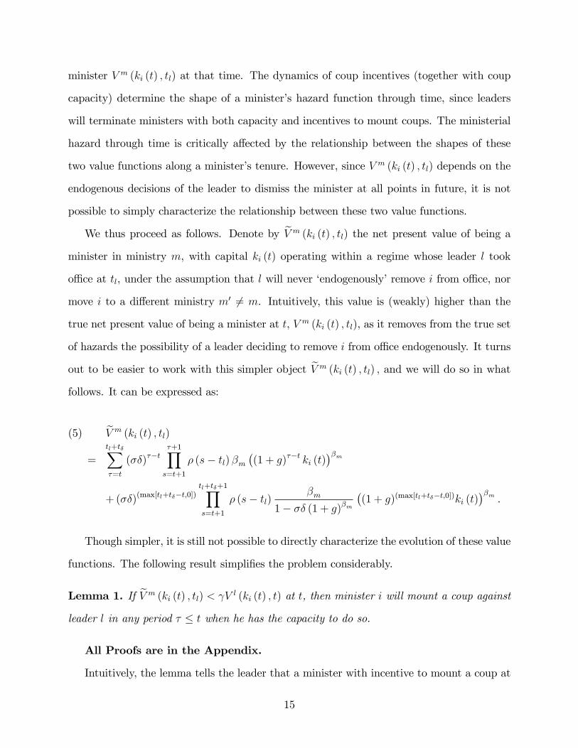
We thus proceed as follows. Denote by eV m (ki (t) ; tl) the net present value of being aminister in ministry m, with capital ki (t) operating within a regime whose leader l took

o¢ ce at tl, under the assumption that l will never �endogenously�remove i from o¢ ce, nor

move i to a di¤erent ministry m0 6= m. Intuitively, this value is (weakly) higher than the

true net present value of being a minister at t, V m (ki (t) ; tl), as it removes from the true set

of hazards the possibility of a leader deciding to remove i from o¢ ce endogenously. It turns

out to be easier to work with this simpler object eV m (ki (t) ; tl) ; and we will do so in whatfollows. It can be expressed as:

eV m (ki (t) ; tl)(5)

=

tl+t�X�=t

(��)��t�+1Ys=t+1

� (s� tl) �m�(1 + g)��t ki (t)

��m+(��)(max[tl+t��t;0])

tl+t�+1Ys=t+1

� (s� tl)�m

1� �� (1 + g)�m�(1 + g)(max[tl+t��t;0])ki (t)

��m .Though simpler, it is still not possible to directly characterize the evolution of these value

functions. The following result simpli�es the problem considerably.

Lemma 1. If eV m (ki (t) ; tl) < V l (ki (t) ; t) at t, then minister i will mount a coup againstleader l in any period � � t when he has the capacity to do so.

All Proofs are in the Appendix.

Intuitively, the lemma tells the leader that a minister with incentive to mount a coup at

15

some future date will also have incentive to mount a coup today, if he has the capacity to

do so. This form of �unraveling�is intuitive. Since coup capacity does not decay, the leader

knows that eventually such a minister will have incentive to act on his current coup capacity.

But if he would do so eventually, he will be dismissed by the leader for certain just before

reaching that speci�c date. Anticipating this dismissal, the minister will act pro-actively

and attempt a coup before that date. Then, the leader, knowing this, will dismiss him �rst,

and so on, up until the �rst date at which a coup capacity ensues.

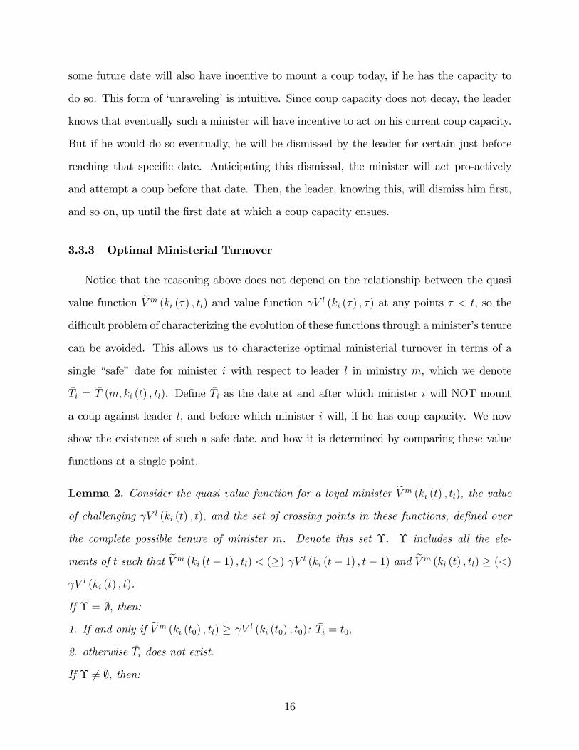
3.3.3 Optimal Ministerial Turnover

Notice that the reasoning above does not depend on the relationship between the quasi

value function eV m (ki (�) ; tl) and value function V l (ki (�) ; �) at any points � < t, so thedi¢ cult problem of characterizing the evolution of these functions through a minister�s tenure

can be avoided. This allows us to characterize optimal ministerial turnover in terms of a

single �safe� date for minister i with respect to leader l in ministry m, which we denote

�Ti = �T (m; ki (t) ; tl). De�ne �Ti as the date at and after which minister i will NOT mount

a coup against leader l, and before which minister i will, if he has coup capacity. We now

show the existence of such a safe date, and how it is determined by comparing these value

functions at a single point.

Lemma 2. Consider the quasi value function for a loyal minister eV m (ki (t) ; tl), the valueof challenging V l (ki (t) ; t), and the set of crossing points in these functions, de�ned over

the complete possible tenure of minister m. Denote this set �. � includes all the ele-

ments of t such that eV m (ki (t� 1) ; tl) < (�) V l (ki (t� 1) ; t� 1) and eV m (ki (t) ; tl) � (<) V l (ki (t) ; t).

If � = ;; then:

1. If and only if eV m (ki (t0) ; tl) � V l (ki (t0) ; t0): �Ti = t0,

2. otherwise �Ti does not exist.

If � 6= ;; then:

16

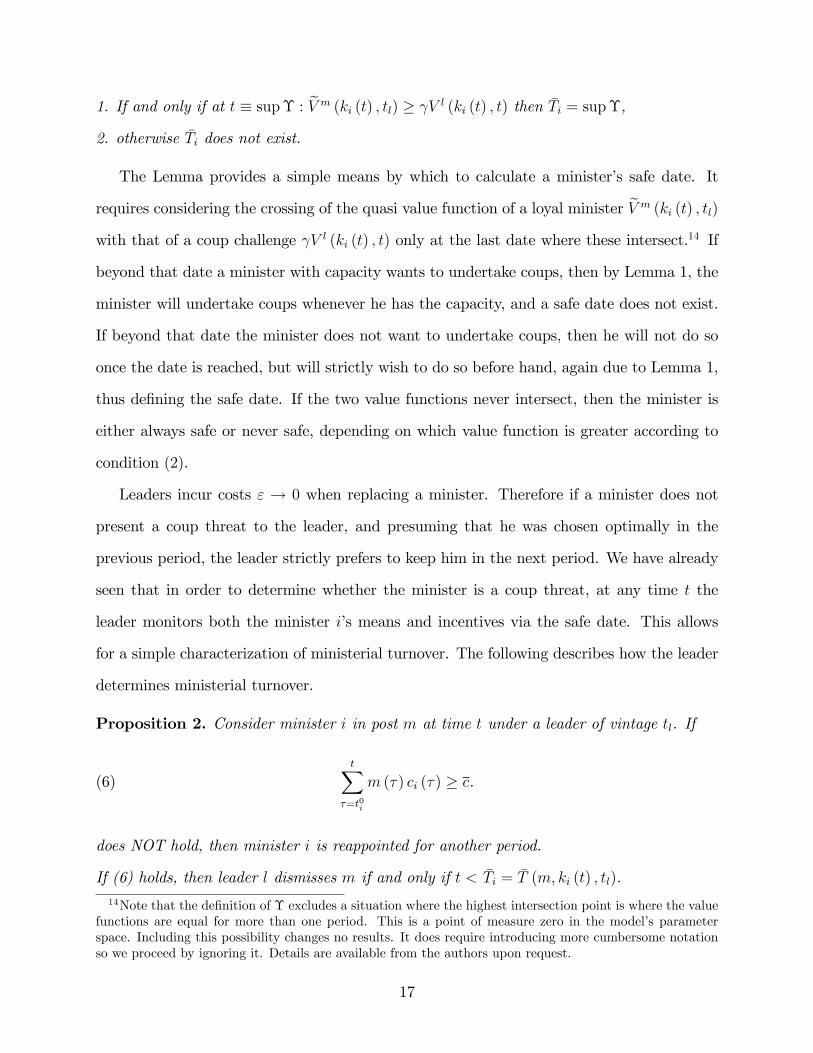
1. If and only if at t � sup� : eV m (ki (t) ; tl) � V l (ki (t) ; t) then �Ti = sup�,2. otherwise �Ti does not exist.

The Lemma provides a simple means by which to calculate a minister�s safe date. It

requires considering the crossing of the quasi value function of a loyal minister eV m (ki (t) ; tl)with that of a coup challenge V l (ki (t) ; t) only at the last date where these intersect.14 If

beyond that date a minister with capacity wants to undertake coups, then by Lemma 1, the

minister will undertake coups whenever he has the capacity, and a safe date does not exist.

If beyond that date the minister does not want to undertake coups, then he will not do so

once the date is reached, but will strictly wish to do so before hand, again due to Lemma 1,

thus de�ning the safe date. If the two value functions never intersect, then the minister is

either always safe or never safe, depending on which value function is greater according to

condition (2).

Leaders incur costs " ! 0 when replacing a minister. Therefore if a minister does not

present a coup threat to the leader, and presuming that he was chosen optimally in the

previous period, the leader strictly prefers to keep him in the next period. We have already

seen that in order to determine whether the minister is a coup threat, at any time t the

leader monitors both the minister i�s means and incentives via the safe date. This allows

for a simple characterization of ministerial turnover. The following describes how the leader

determines ministerial turnover.

Proposition 2. Consider minister i in post m at time t under a leader of vintage tl. If

(6)tX

�=t0i

m (�) ci (�) � c.

does NOT hold, then minister i is reappointed for another period.

If (6) holds, then leader l dismisses m if and only if t < �Ti = �T (m; ki (t) ; tl).14Note that the de�nition of � excludes a situation where the highest intersection point is where the value

functions are equal for more than one period. This is a point of measure zero in the model�s parameterspace. Including this possibility changes no results. It does require introducing more cumbersome notationso we proceed by ignoring it. Details are available from the authors upon request.

17

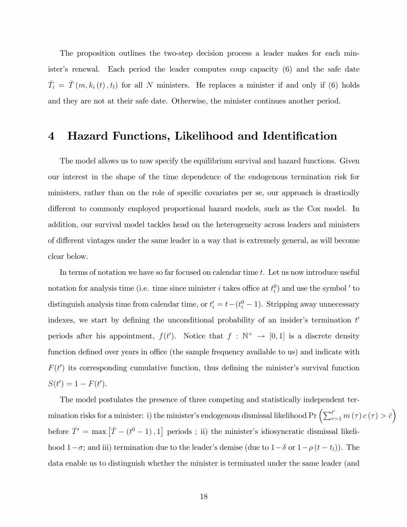
The proposition outlines the two-step decision process a leader makes for each min-

ister�s renewal. Each period the leader computes coup capacity (6) and the safe date

�Ti = �T (m; ki (t) ; tl) for all N ministers. He replaces a minister if and only if (6) holds

and they are not at their safe date. Otherwise, the minister continues another period.

4 Hazard Functions, Likelihood and Identi�cation

The model allows us to now specify the equilibrium survival and hazard functions. Given

our interest in the shape of the time dependence of the endogenous termination risk for

ministers, rather than on the role of speci�c covariates per se, our approach is drastically

di¤erent to commonly employed proportional hazard models, such as the Cox model. In

addition, our survival model tackles head on the heterogeneity across leaders and ministers

of di¤erent vintages under the same leader in a way that is extremely general, as will become

clear below.

In terms of notation we have so far focused on calendar time t. Let us now introduce useful

notation for analysis time (i.e. time since minister i takes o¢ ce at t0i ) and use the symbol0 to

distinguish analysis time from calendar time, or t0i = t�(t0i � 1). Stripping away unnecessary

indexes, we start by de�ning the unconditional probability of an insider�s termination t0

periods after his appointment, f(t0). Notice that f : N+ ! [0; 1] is a discrete density

function de�ned over years in o¢ ce (the sample frequency available to us) and indicate with

F (t0) its corresponding cumulative function, thus de�ning the minister�s survival function

S(t0) = 1� F (t0).

The model postulates the presence of three competing and statistically independent ter-

mination risks for a minister: i) the minister�s endogenous dismissal likelihood Pr�Pt0

�=1m (�) c (�) > �c�

before �T 0 = max��T � (t0 � 1) ; 1

�periods ; ii) the minister�s idiosyncratic dismissal likeli-

hood 1��; and iii) termination due to the leader�s demise (due to 1�� or 1�� (t� tl)). The

data enable us to distinguish whether the minister is terminated under the same leader (and

18

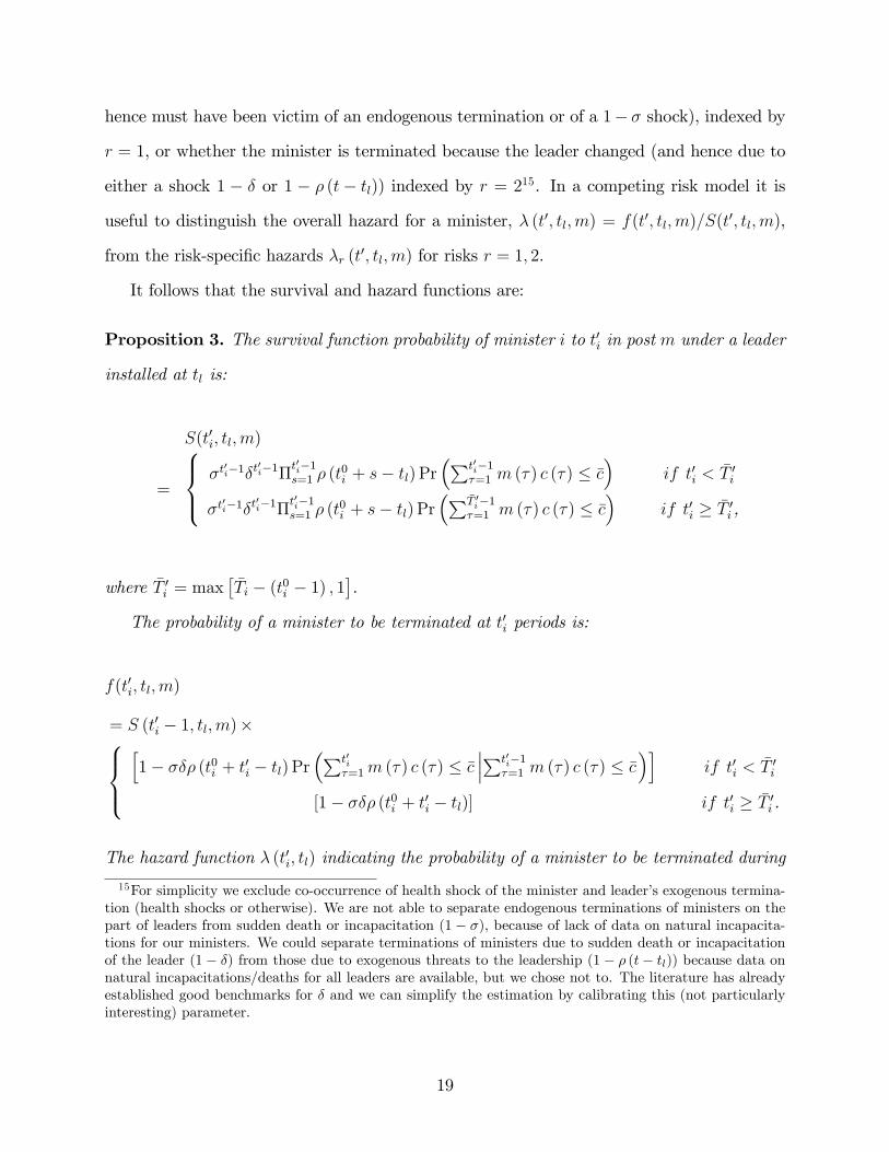
hence must have been victim of an endogenous termination or of a 1� � shock), indexed by

r = 1, or whether the minister is terminated because the leader changed (and hence due to

either a shock 1 � � or 1 � � (t� tl)) indexed by r = 215. In a competing risk model it is

useful to distinguish the overall hazard for a minister, � (t0; tl;m) = f(t0; tl;m)=S(t0; tl;m),

from the risk-speci�c hazards �r (t0; tl;m) for risks r = 1; 2.

It follows that the survival and hazard functions are:

Proposition 3. The survival function probability of minister i to t0i in post m under a leader

installed at tl is:

S(t0i; tl;m)

=

8><>: �t0i�1�t

0i�1�

t0i�1s=1 � (t

0i + s� tl) Pr

�Pt0i�1�=1 m (�) c (�) � �c

�if t0i <

�T 0i

�t0i�1�t

0i�1�

t0i�1s=1 � (t

0i + s� tl) Pr

�P �T 0i�1�=1 m (�) c (�) � �c

�if t0i � �T 0i ,

where �T 0i = max��Ti � (t0i � 1) ; 1

�.

The probability of a minister to be terminated at t0i periods is:

f(t0i; tl;m)

= S (t0i � 1; tl;m)�8><>:h1� ��� (t0i + t0i � tl) Pr

�Pt0i�=1m (�) c (�) � �c

���Pt0i�1�=1 m (�) c (�) � �c

�iif t0i < �T 0i

[1� ��� (t0i + t0i � tl)] if t0i � �T 0i .

The hazard function � (t0i; tl) indicating the probability of a minister to be terminated during

15For simplicity we exclude co-occurrence of health shock of the minister and leader�s exogenous termina-tion (health shocks or otherwise). We are not able to separate endogenous terminations of ministers on thepart of leaders from sudden death or incapacitation (1 � �), because of lack of data on natural incapacita-tions for our ministers. We could separate terminations of ministers due to sudden death or incapacitationof the leader (1 � �) from those due to exogenous threats to the leadership (1 � � (t� tl)) because data onnatural incapacitations/deaths for all leaders are available, but we chose not to. The literature has alreadyestablished good benchmarks for � and we can simplify the estimation by calibrating this (not particularlyinteresting) parameter.

19

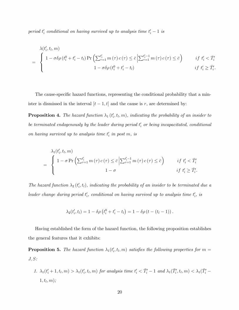
period t0i conditional on having survived up to analysis time t0i � 1 is

�(t0i; tl;m)

=

8><>: 1� ��� (t0i + t0i � tl) Pr�Pt0i

�=1m (�) c (�) � �c���Pt0i�1

�=1 m (�) c (�) � �c�

if t0i <�T 0i

1� ��� (t0i + t0i � tl) if t0i � �T 0i .

The cause-speci�c hazard functions, representing the conditional probability that a min-

ister is dismissed in the interval [t� 1; t] and the cause is r, are determined by:

Proposition 4. The hazard function �1 (t0i; tl;m), indicating the probability of an insider to

be terminated endogenously by the leader during period t0i or being incapacitated, conditional

on having survived up to analysis time t0i in post m, is

�1(t0i; tl;m)

=

8><>: 1� � Pr�Pt0i

�=1m (�) c (�) � �c���Pt0i�1

�=1 m (�) c (�) � �c�

if t0i < �T 0i

1� � if t0i � �T 0i .

The hazard function �2 (t0i; tl), indicating the probability of an insider to be terminated due a

leader change during period t0i, conditional on having survived up to analysis time t0i, is

�2(t0i; tl) = 1� ��

�t0i + t

0i � tl

�= 1� �� (t� (tl � 1)) .

Having established the form of the hazard function, the following proposition establishes

the general features that it exhibits:

Proposition 5. The hazard function �1(t0i; tl;m) satis�es the following properties for m =

J; S:

1. �1(t0i + 1; tl;m) > �1(t0i; tl;m) for analysis time t

0i <

�T 0i � 1 and �1( �T 0i ; tl;m) < �1( �T 0i �

1; tl;m);

20

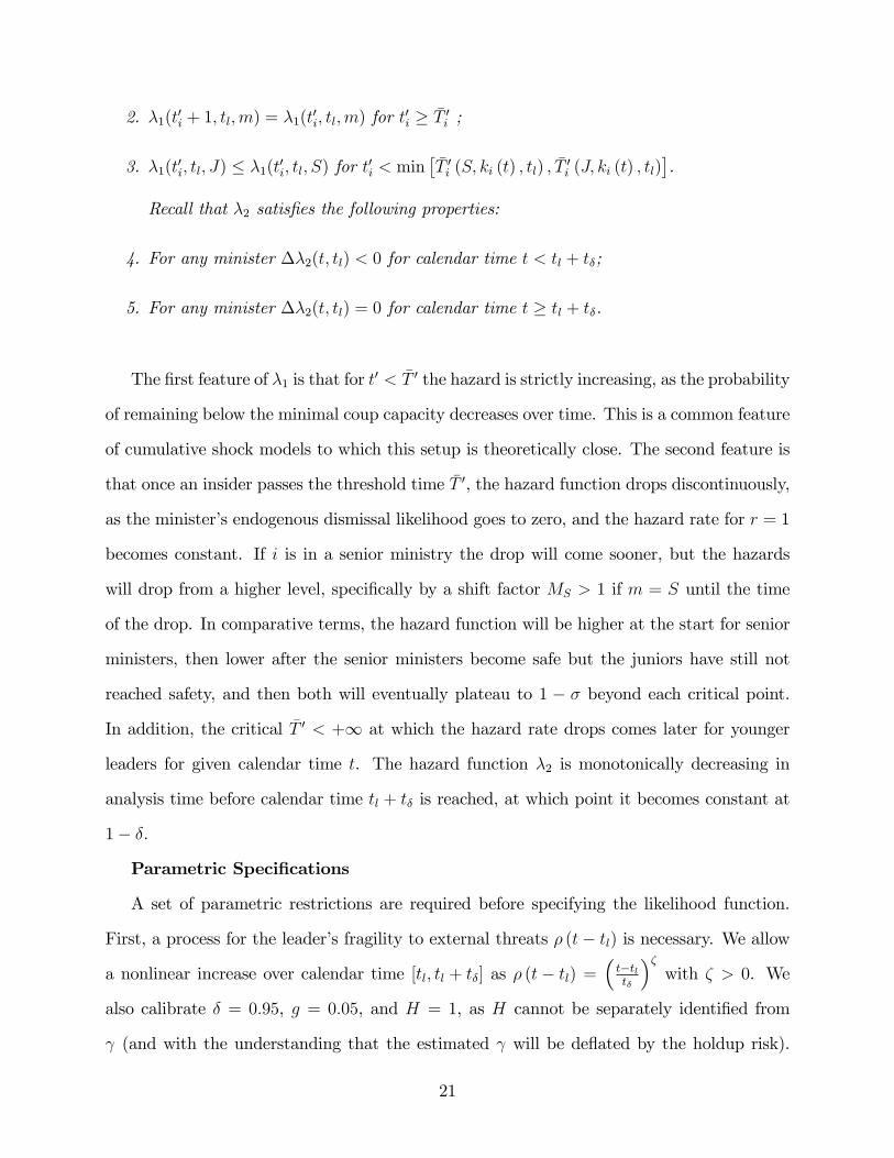
2. �1(t0i + 1; tl;m) = �1(t0i; tl;m) for t

0i � �T 0i ;

3. �1(t0i; tl; J) � �1(t0i; tl; S) for t0i < min��T 0i (S; ki (t) ; tl) ; �T

0i (J; ki (t) ; tl)

�.

Recall that �2 satis�es the following properties:

4. For any minister ��2(t; tl) < 0 for calendar time t < tl + t�;

5. For any minister ��2(t; tl) = 0 for calendar time t � tl + t�.

The �rst feature of �1 is that for t0 < �T 0 the hazard is strictly increasing, as the probability

of remaining below the minimal coup capacity decreases over time. This is a common feature

of cumulative shock models to which this setup is theoretically close. The second feature is

that once an insider passes the threshold time �T 0, the hazard function drops discontinuously,

as the minister�s endogenous dismissal likelihood goes to zero, and the hazard rate for r = 1

becomes constant. If i is in a senior ministry the drop will come sooner, but the hazards

will drop from a higher level, speci�cally by a shift factor MS > 1 if m = S until the time

of the drop. In comparative terms, the hazard function will be higher at the start for senior

ministers, then lower after the senior ministers become safe but the juniors have still not

reached safety, and then both will eventually plateau to 1 � � beyond each critical point.

In addition, the critical �T 0 < +1 at which the hazard rate drops comes later for younger

leaders for given calendar time t. The hazard function �2 is monotonically decreasing in

analysis time before calendar time tl + t� is reached, at which point it becomes constant at

1� �.

Parametric Speci�cations

A set of parametric restrictions are required before specifying the likelihood function.

First, a process for the leader�s fragility to external threats � (t� tl) is necessary. We allow

a nonlinear increase over calendar time [tl; tl + t�] as � (t� tl) =�t�tlt�

��with � > 0. We

also calibrate � = 0:95, g = 0:05, and H = 1, as H cannot be separately identi�ed from

(and with the understanding that the estimated will be de�ated by the holdup risk).

21

The baseline exogenous ministerial shock is set at � = 0:9016. Further, and in order to

maximize data availability for the estimation of the model�s parameters we impose complete

symmetry among junior and senior posts, MS = 1 and �m = � for m = J; S. Hence the

parameter identi�es a single safe date �T (m; ki (t) ; tl) m = J; S common to all ministers

under leader l and we can show that in this case no information about the exact value of the

political capital levels kl or ki is necessary to evaluate the incentive compatibility constraints

of ministers that determines �T .

For minister i under leader of vintage tl observed to leave the cabinet after t0i periods due

to risk r, de�ne the dummy di = 1 if i is not right censored17 and 0 otherwise, and the dummy

ri = 1 if i is terminated by risk 1 and 0 otherwise. De�ne the set of structural parameters of

the desire and capacity functions � = (�; t�; �; ; &c). While parameters (�; t�; �) are going

to be assumed constant across countries and leaders, we are going to allow the parameter &c

to di¤er across countries (allowing the accumulation of coup capacity to vary at the national

level and indicating it in bold as a vector) and the parameter to vary at the country-leader

level (allowing the coup success likelihood to vary from regime to regime).

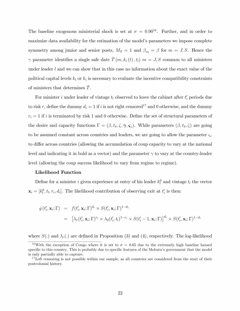
Likelihood Function

De�ne for a minister i given experience at entry of his leader k0l and vintage tl the vector

xi = [k0l ; tl; ri; di]. The likelihood contribution of observing exit at t

0i is then:

g (t0i;xi; �) = f(t0i;xi; �)di � S(t0i;xi; �)1�di

=��1(t

0i;xi; �)

ri � �2(t0i; tl)1�ri � S(t0i � 1;xi; �)�di � S(t0i;xi; �)1�di

where S(:) and �r(:) are de�ned in Proposition (3) and (4), respectively. The log-likelihood

16With the exception of Congo where it is set to � = 0:65 due to the extremely high baseline hazardspeci�c to this country. This is probably due to speci�c features of the Mobutu�s government that the modelis only partially able to capture.17Left censoring is not possible within our sample, as all countries are considered from the start of their

postcolonial history.

22

for a sample i = 1; :::; I of ministerial spells18 is then:

(7) L (�;�;�) =IXi=1

ln g (t0i;xi; �) .

Identi�cation

The apparently simple formulation (7) is deceptive. First, much of the identi�cation

here relies on the unobserved safe dates �T 0i which impose stark discontinuities to the hazard

functions. Second, hazard functions are heterogenous across ministers of di¤erent vintages.

To see this, consider a leader with a safe date six years from the time he was installed.

Minister A installed at the same time as the leader faces a di¤erent hazard function than

minister B installed �ve periods into the leader�s tenure. At year 1 of his tenure A faces

six periods of endogenous risk ahead. At year 1 of his tenure B (already �ve periods closer

to the safe date) faces only one period of endogenous termination risk. Interestingly, the

pooling of ministers at di¤erent distance from a safe date, each with a discontinuous hazard

function as in (5), is precisely what allows the model to �t the smooth hump-shaped hazard

functions in Figure 5. This is because, by changing the safe date, the underlying mixture of

individuals deemed safe versus still exposed to risk 1 at each t0 changes.

For identi�cation, we can take advantage of the useful separability of our problem. We

do not observe the amount of political capital of each minister ki (t), but we have handy

observational proxies of political capital for ministers and leaders. De�ne the observed

cumulated experience in government (i.e. number of years served in any cabinet capacity) at

calendar time t by minister i, ~ki (t) and likewise for the leader l, ~kl (t). We can realistically

18With a slight abuse of notation we indicate with i both the minister and ministerial spells. Typicallyministers present only one spell, but certainly not always. The implication in the loglikelihood (7) is thatwe consider here separate spells of the same minister as di¤erent observations with respect to the draws of� and the initial level of the coup network stock. However, we do maintain memory of the experience of theminister through the initial political capital stock k0i , which also in�uences the coup incentives and is higherat every subsequent spell of the same individual.

23

posit that years of experience are a noisy, but unbiased, proxy of political capital:

kl (t) = ~kl (t) + "lt

kmi (kl (t)) = ~ki (t) + "it

where " is a mean zero error uncorrelated across individuals. Recall that at any date t the

model implies ki (kl (t)) =kl (t) = �= (1� �) as a steady relationship between ministerial and

leader�s political capital19. By rearranging and pooling across all leaders/countries in our

sample l and all i at tl it is therefore possible to estimate:

(8) ~ki (tl) =�

1� �~kl (tl) + 'ltl + "

�itl

where 'ltl =�1��"ltl is a leader-speci�c �xed e¤ect. The auxiliary regression (8) is particularly

useful as it directly delivers estimates for �̂ independently of the other parameters of the

model.

Further, the parameters (t�; �) governing the hazard �2 can also be directly recovered

by �tting a parametric hazard model to the leaders�termination data alone (the same data

used in Figure 1 and 2 to be precise).

Given the common parameters (�; t�; �), the vectors of coup success and coup capacity

parameters ( ; &c) governing the hazard �1 are estimated postulating a safe date for each

19Although apparently restrictive, the result of constant capital across ministries of type m is a necessarycondition for dealing parsimoniously with the lack of clear proxies of political capital of government insid-ers. Such a metric would be arduous to de�ne for democratic regimes, where political data is much moretransparent and readily available than in Africa, but it is even more so in this context. Clearly the observedcumulated experience in government of any politician is only one partial dimension of his/her political cap-ital. Focusing only on previous years in government as a measure of political experience of a minister couldunderestimate the e¤ective level of political capital. For instance, experience as a party cadre or within par-ticular pre-colonial ethnic institutions (i.e. the role of paramount chiefs in Sierra Leone) are hard to measure,but surely a factor in determining the amount of political capital of leaders and insiders. Our approach is toleverage on multiple observations of career ministers over time in order to pin down the patterns of averagepolitical experience within the dictator�s inner circle. This obviously sacri�ces some heterogeneity acrossministers along the ki (t) dimension, but it is the consequence of paucity of accurate proxies for ki (t). Partof this heterogeneity is however recovered in estimation by allowing for country-speci�c parameters.

24

leader and iterating until a global maximum of the likelihood function is obtained 20.

5 Estimation

Table 3a reports the maximum likelihood estimates for all countries. One �rst important

parameter that is estimated through the ministerial data is the technological parameter �,

which also identi�es the bargaining power of the leader relative to his cabinet insiders. We

impose a common � for all countries. Diminishing returns to ministerial political capital

appear to kick in very early in the data, as the estimated � = 0:055 imposes a substantial

degree of curvature in the production function. This implies a relative insensitivity of the

political production process to the experience of the minister. Consequently, in our sample

the bargaining power of the minister appears low. The bargaining power of the leader can

be computed as � = 0:945 relative to ministers.

The country-speci�c coup capacity parameter &c and leader-speci�c coup success prob-

ability are essential in determining whether a country exhibits a safe date or not. The

absence of a safe date implies the hazard of ministers to be monotonically increasing, as per

Proposition 5. If a leader exhibits a safe date, the hazard is non monotonic.

The estimates for &c are indicative of the speed at which the coup capacity threshold

(6) is met by a government insider. this parameter governs the steepness of the hazard

function. Speci�cally, &c identi�es the scale of the exponential shocks to the capacity of

staging coups, or the speed at which ministers might be building a �power base� (Soest,

2007). The higher &c the faster coup capacity accumulates and the faster the leader is bound

to �re his ministers. The range of &c is varied. For example, the �musical chairs�of Mobutu

Sese�s Congo generate a high estimate of 0:61, implying extremely high churning. The more

stable Cameroon has a value of 0:36. To see why a scale of 0:61 would imply a high value of

20Given the parsimony of our model, the likelihood function depends on a relatively small number ofparameters. This allows for a fairly extensive search for global optima over the parametric space. Inparticular, we employ a genetic algorithm optimizer.

25

churning one has to compute the expected time at which a threshold of 1 is reached21 by the

convolution of the coup capacity c shocks. Since the scale of an exponential located at 0 is

its expected value, then in Congo there�s an accumulation of 0:61 per period, or equivalently

the threshold for coup capacity may be reached in less than 2 years on average. Instead, for

&c = :36 the threshold is reached in about 3 years, and so on. Obviously these �gures imply

sharply decreasing survival functions, as discussed below.

The vector is the most complex part of the parameter space to pin down due to the

sharp discontinuity presented by (1). We are however able to identify the parameters in

Montecarlo simulations. Given the discreteness of the safe date (measured in years), there is

an interval of coup success probabilities satisfying the condition in Lemma 1 and each can

only be set identi�ed. In part b of Table 3 we report the lower and upper bound on interval

of the parameters for each leader, ordered over time and by country. In case ministers

under a leader are never safe (i.e. they always have an incentive to stage coups), the interval

includes the extreme 1 (i.e. coups succeeding surely cannot be ruled out). As an example

for how to read Table 3b, Ahmadou Ahidjo corresponds to the �rst leader of Cameroon and

has a in a tight neighborhood of 0:10 percent, while Paul Biya, Cameroon�s second leader,

has a in a tight neighborhood of 0:13 percent, and so on.

The parameter ranges from 0:1 to 0:25 percent typically. This does not obviously imply

implausibly unlikely coup successes, as one has to remember that this �gure has to be scaled

by H. Speci�cally, the reported bounds on the elements of are obtained as the likelihood

of success of a coup against that leader multiplied by the holdup probability H. Given that

each and H are both unobservable and related to the (also unobservable) safe date �T , it

is hard to pin down the exact strength of the coup threat quantitatively. What is reassuring

is that the estimates appear larger in countries with more troubled histories of coups and

plotting like Congo and Nigeria, than in countries with relatively more stable autocratic

governments, like Gabon and Cameroon.

211 is in fact our normalized value for the coup capacity threat level �c.

26

Table 3a also reports the leader�s hazard parameters. We impose a common vector (t�; �)

for all countries, given the typical paucity of leaders per country which would make an

estimation by country impossible. Leaders reach a point of constant low hazard � after

t� = 15 years in o¢ ce and along the way we observe a smooth drop in regime fragility

(� = 0:0567). Both are very tightly estimated parameters.

Concerning the �t, the model is able to capture the non-monotonic nature of the termi-

nation hazard functions in countries with safe dates, while accommodating monotonically

increasing hazard functions in the remaining countries which do not exhibit safe dates. In

Appendix Figure A1 we report the model �t for all countries as well as the nonparametric

hazard �t. The model also o¤ers remarkably good �t of the survival functions of the min-

isters also reported for each country separately in Appendix Figure A2. Survival functions

are obviously very important to the estimation of the overall duration of each minister, as

evident from our likelihood function, so it is reassuring the �t is tight along this dimension

as well.

An important check we perform on our model is to restrict estimation exclusively to min-

isters in top cabinet positions22. In Appendix Tables A1a and A1b we report the maximum

likelihood estimates restricting the sample to the senior ministerial posts only. Given that

senior ministers are the most plausible source of replacement risk for the leader, one may

want to make sure that the estimated parameters do not vary wildly relative to the baseline

and the �t remains reasonable. In fact, were the estimates extremely unstable relative to

the baseline, this might be a source of concern, given the focus on a subset of the data

where coup concerns should be more salient. Tables A1(a,b) are reassuring in this sense,

as the implications of Table 3(a,b) are largely con�rmed, with one model�s points estimates

typically within con�dence bands of the other speci�cation.

22As de�ned in Section 2.

27

6 Alternative Duration Models

This section discusses a set of relevant alternatives relative to our main model. The goal

is to provide support for our modeling choices by rejecting competing theoretical mechanisms

that do not match the data.

Consider �rst what is, likely, the most intuitive of all alternatives: leaders are tantamount

to employers hiring workers and try to select the best ministers, laying o¤ the rest. This is

a pure selection mechanism of ministerial personnel based on learning workers�type/match

quality on the part of the leader. Without providing an explicit microfoundation, which

would be redundant, the idea of a selection motive a¤ecting termination risks for ministers

works through the screening of the minister�s types. Early on in their tenure low quality

ministers are to be screened out and only talented ministers stay.

It is well known that selection delivers a downward-sloping hazard function over time

in o¢ ce under the same leader. This is amply discussed in the vast (and related) labor

economics literature concerned with job separations in duration models of employment (so

called �inspection good models�with no gradual learning about the employer-employee match,

Jovanovich, 1984). Where we can safely reject this alternative is in that it would fail to

predict increasing hazard rates, which we have shown previously to be a pervasive feature of

the data23.

More formally, these alternative mechanisms of selection or learning by doing can be

accommodated in our empirical model and tested through generalized likelihood ratio tests,

such as the Vuong and the Clarke speci�cation selection tests. Such tests are specif-

ically designed to test non-nested models in a maximum likelihood environment24. To

23This very same fact rejects as an alternative mechanism learning by doing on the part of ministersas well. That is, a setting in which early on in his career a ministers makes a lot of mistakes that couldpotentially cost him his job, but whose likelihood decreases as he gets more acquainted with his role overtime. Again the predicted equilibrium hazard function would be downward sloping in analysis time underthis alternative scenario (see Nagypal, 2007).24The null hypotheses for both the Vuong and Clarke tests are that both our model and the alternative

mechanism are true against a two-sided alternative that only one of the two models is in fact true. TheVuong test has better power properties when the density of the likelihood ratios of the baseline and thealternative is normally distributed, while the Clarke test is more powerful when this condition is violated.

28

see how implementing such tests is possible, consider the endogenous dismissal likelihood

Pr�Pt0

�=1m (�) c (�) > �c�. This is essentially the backbone of a cumulative shock model

with a resistance threshold �c. Now, let us augment the process of accumulation of shocks by

adding n additional shocks, g (�), for the �rst � � m periods in o¢ ce and by adding no addi-

tional shocks after m periods. These additional early shocks essentially load risk of passing

the resistance threshold �c in the �rst few years of a minister�s career and can potentially de-

scribe an early selection hazard in addition to the coup risk which is the focus of our model.

The useful convolution properties of the shock distributions that we have emphasized above

can be preserved if one is willing to maintain the assumption of i.i.d. exponential shocks for

g. In Table 4 we consider three di¤erent instances of the selection mechanism, by imposing

n = 1; 2; and 5 additional shocks g are added in period m = 1 only. This means that the

hazard function can now be construed using Pr�Pt0

�=1m (�) c (�) + ng (1) > �c�, regulating

the intensity of the selection strength by increasing n. Were the data willing to accom-

modate additional selection risk in the �rst year of o¢ ce, as the Jovanovich model would

imply for example, then Vuong and Clarke tests would support such an alternative relative

to the simple hazard process implied by our model. As is evident from Table 4, all three

alternative models are rejected in favor of our baseline mechanism. All tests favor rejection

with p-values less than 1 percent. Table 4 indicates that these additional mechanism play

at best a second order role.

A di¤erent selection mechanism can also be addressed. Let us assume, for instance, that

a leader has only partial information about the true political quality of his ministers, but

observes informative signals slowly over time. Under rational learning, the accumulation

of information would imply some delay in �ring ministers, due to the likely use of optimal

thresholds in posterior beliefs for determining, with a su¢ cient degree of certainty, a rational

selection criterion. This particular setup can deliver a selection with delay hazard function.

As it takes time to assess the (initially unknown) quality of every minister in order to select

the �good�ministers and drop the �bad�, initially increasing hazards could be generated in

29

equilibrium, while a hazard drop later on could be a simple consequence of the selection

dynamics described above25.

Where this mechanism would fail empirically is in matching an important feature of the

data: the fact that more experienced leaders tend to systematically hire more experienced

ministers and less senior leaders tend to hire less experienced ministers. In fact, any model

pivoting around selection incentives based on discovering the true type of a minister would

likely imply a preference for more experienced ministers by both experienced and unexperi-

enced leaders alike, for experienced ministers are, in many respects, a better known entity.

This appears at variance with the data.

This last remark points to a more basic empirical �aw of selection mechanisms based on

�xed ministerial types. Were low quality ministers to be discarded and high quality ones

retained, a minister that had been terminated should never reappear in government. In fact,

such a minister must have been terminated because her or his true type had been revealed

with su¢ cient precision and s/he turned out to be bad. Contrary to such a prediction,

around 33:4 percent of the ministers at the beginning of a leader�s regime exhibit some

previous experience in government, i.e. multiple ministerial spells. This appears somewhat

at odds with the core idea of a selection mechanism.

A �nal reasonable alternative mechanism for the process of political appointment in

neopatrimonialist systems, like the ones in Africa, is what can be referred to as the �my turn

to eat�hypothesis26. In the words of van Soest (2007) �neopatrimonial rulers frequently rotate

the political elite [...] in order to extend the clientelist network�, while Snyder (1992) states

that �Mobutu�s patronage network was characterized by such frequent circulation of elites

that Thomas Turner likened Zaire�s politics to a �game of musical chairs�. Elite circulation

25Non-monotone hazard rates (�rst increasing and eventually decreasing over tenure) are common inmodels with job-matching where the quality of the match is unknown at the time of the match formationand is revealed over time through observing one�s productivity on the job. See Jovanovic (1979, 1984) forearly examples within the labor economics literature. Another stream of the literature focusing on agencyproblems in political environment focuses on the unwillingness of agents to reveal information, also producingnon-monotonic hazard functions, as in Aghion and Jackson (2014).26We thank Leonard Wantchekon at Princeton University for suggesting this alternative.

30

atomized Zairian elites by pressuring them to focus exclusively on self-aggrandizement during

the short period they had access to state power and perquisites.�Turner and Young (1985),

cited by Acemoglu, Robinson, and Verdier (2004), speci�cally talk with respect to Mobutu

of �Client o¢ ce holders have been constantly reminded of the precariousness of tenure by the

frequency of o¢ ce rotation, which simultaneously fuels the hopes of those Zairians anxiously

waiting just outside the portals of power�. More precisely, suppose there is a set of political

elites that a country leader has to �feed� with patronage disbursements waiting on the

national cabinet�s sidelines and that ministerial posts precisely serve this purpose, as vastly

documented (Arriola, 2009; Francois, Rainer, and Trebbi, 2014). Essentially, elites are

to be assigned positions, be fed, and eventually let go. This mechanism would arguably

predict initially increasing hazard rates, as it takes time to extract patronage. But again

this logic struggles empirically along two dimensions. First, �my turn to eat�would hardly

�t the eventual decreasing hazards, as the likelihood of a politician being satiated and let go

should reasonably increase over time. Modulo additional ad-hoc mechanisms, this alternative

interpretation would also fail to directly match why more experienced leaders tend to hire

more experienced ministers, as evident in Section 2.

7 Counterfactual Exercises and Welfare

This section explores some important quantitative implications of our model. A critical

implication of our theory is that the incentives for leadership survival may be playing a fun-

damental role in a¤ecting the political horizons of SSA ministers. While we do not model

formally how shorter horizons translate in to lower levels of political investment, there is the-

oretical and empirical evidence in support of this mechanism. Prominently, a vast theoretical

literature pivots on myopic behavior of politicians when subject to electoral or political risk

shortening their horizon (Amador, 2012; Aguiar and Amador, 2011). Empirically, Dal Bo

and Rossi (2011) show precise quasi-experimental evidence of curtailed political investment

31

in the context of the Argentine Congress.

This section explores some relevant counterfactual exercises that can guide our under-

standing of the quantitative drivers of average ministerial lifetimes in o¢ ce. Table 5 reports

four sets of counterfactuals for each country in our sample, in addition to the average minister

lifetime under the baseline model (for reference).

The �rst parameterization we explore is an increase in the bargaining power of ministers

versus the leader. We increase the technological parameter � by 10 percent of its estimated

value. By reducing the gap between what is captured by the minister and the leader, lead-

ership becomes less appealing and the loyalty of a minister easier to maintain. Intuitively,

this reduces incentives for terminating insiders and the average length of o¢ ce increases

�sometimes substantially, as in Cameroon where it adds a full extra year in o¢ ce to the

typical minister. The reader may think of several policies aimed at adding value to the

political capital and the experience of a minister in o¢ ce that may slow down the setting in

of diminishing returns and may increase �. These include administrative training programs

or international exchanges for the requali�cation of top bureaucrats, for example.

Increases in the speed of coup capacity accumulation or higher likelihood of coup success

(respectively, &c and ,both increased by 10% of their baseline values) drastically shorten

average ministerial horizons. This is a symmetric e¤ect relative to that discussed above. By

increasing the coup threat stemming from ministers, one forces leaders toward more minis-

terial churning, strongly reducing their political horizons (and possibly increasing political

myopia). These results give perspective to the indirect political e¤ects stemming from covert

or explicit foreign interventions in the African continent during the Cold War period, many

of which were re�ected in aid to the planning and implementation of coups. Francois, Rainer,

and Trebbi (2014) consider, for instance, the role of France in West Africa and the role of

the United States and Soviet Union in drastically shaping threats to the leadership of SSA

countries during the Cold War. Table 5�s results strongly complement that intuition.

In the last row, Table 5 reports the e¤ects of shortening the phase of exogenous leader

32

fragility, t�. Interestingly, this reduction, by increasing the value of the leadership, makes

coup threats more prominent and leads to shorter average ministerial tenures. Again, the

counterfactual indicates how arti�cially induced stability of leaders (e.g. foreign protection

of certain African strongmen, including Mobutu Sese Seko) may trickle down through the

political organization of the regime.

While Table 5 emphasizes the potential drivers of ministerial churning, Table 6 reports the

percent output losses due to the employment of suboptimal cabinets on the part of national

leaders in our sample. The choice of weaker ministers due to their low bargaining strength

is, in fact, an important feature of our model. Table 6 shows that such welfare losses can

be substantial. If one were to endow every leader in each country with the most productive

cabinet observed in that country over our time period and use the estimated political capital

levels induced by (8), gains hovering around 30 percent of the total political output of the

cabinet in a given year could be achievable. There is also vast variation in the magnitude of

such welfare losses. The welfare losses range from a minimum of 16:8 percent of total output

in Cote d�Ivoire to a maximum of 80:5 percent in Gabon. As we have emphasized in Section

4 of the paper, the balance of strength between the leader and the ministers is the source of

these losses.

8 Conclusions

This paper studies the cabinet survival of national ministers in a sample of �fteen sub-

Saharan countries since independence. We show that the hazard risks of termination of

cabinet members display increasing hazard rates, particularly over the �rst �ve years in

o¢ ce, a strikingly di¤erent pattern from that found in the same continent for hazard risks

of national leaders (which are typically decreasing in analysis time).

We show that this speci�c pattern of time dependency can be successfully rationalized

by a model in which leaders optimally select and dismiss cabinet members based on their

33

value (in terms of ministerial output) and on their threat as a potential replacement for the

leader.

The model provides a complete parametric representation of the ministerial hazard func-

tions, which we then estimate structurally to derive information on the bargaining problem

between the leader and his ministers and on the dynamic process of coup capacity accumula-

tion in these regimes. The �t of the model in terms of hazard risks and survival probabilities

is excellent and the model performs well when pitted against several relevant theoretical

alternatives. We further show that the welfare losses related to ministerial bargaining are

substantial.

Overall, these �ndings speak directly to the debate on systematic political failure in

Africa. While the continent�s recent economic history is replete with political failures taking

many forms, from civil con�ict to patrimonialism, some of these failures have been ascribed

directly to a political class that appears myopic and rapacious. This, we postulate, may

just be a result of the speci�c institutional environment in which both ministers and leaders

operate: an environment in which power is transferred through bloodshed and is particularly

threatening to leaders. Such threats translate to rapidly increasing dismissal probabilities

for insiders. We believe that this paper, by highlighting the role of leadership survival as

central to the institutional organization of African governments, presents a novel mechanism

in the analysis of political incentives in these weakly institutionalized systems.

34

9 Appendix

Proof of Lemma 1

Proof. Since eV m (ki (t) ; tl) � V m (ki (t) ; tl) ; eV m (ki (t) ; tl) < V l (ki (t) ; t) implies V m (ki (t) ; tl) < V l (ki (t) ; t) : Minister m has incentive to mount a coup against l in period t; and will do soifPt

�=t0im (�) ci (�) � c, i.e., he has the capacity at time t: Now consider period t� 1; and

suppose thatPt�1

�=t0im (�) ci (�) � c, i.e., minister i has capacity to mount a coup against l

then. Since ci (t) is drawn from C; which has non-negative support, i will also have capacityto mount a coup against l in t: Thus, leader l will dismiss i from the ministry in t, sincehe would mount a coup with certainty if he were to remain. A minister dismissed at t willnever re-enter under the current leader because, from (3) ; kmi (kl) =

�m1��m

kl; and kl growsat 1+ g per period, whereas a dismissed minister�s capital does not grow when out of o¢ ce.Consequently, minister m will attempt a coup at the end of period t � 1: Since m0s coupcapacity and experience are public knowledge, l will dismiss m at the start of period t� 1:Notice that this result does not depend on the relationship between eV m (ki (t� 1) ; tl) and V l (ki (t� 1) ; t� 1) ; and follows only from eV m (ki (t) ; tl) < V l (ki (t) ; t) and the fact ofcoup capacity at t�1: Consequently, in period t�2; if m has coup capacity then, he will alsohave it in t�1; and therefore in t. He will be dismissed at the start of t�1; and by identicalreasoning, he will thus be dismissed at the start of t�2: The same argument can be applied toperiod t�3 and so on up to the �rst period, denote it t1; at which

Pt1�=t0i

m (�) ci (�) � c:�

Proof of Lemma 2

Proof. Suppose � = ;: Then eV m (ki (t0) ; tl) � V l (ki (t0) ; t0) implies eV m (ki (t) ; tl) � V l (ki (t) ; t)8t > t0. Then, provided eV m (ki (t) ; tl) = V m (ki (t) ; tl) holds, minister i hasnever an incentive to mount a coup against l. But a necessary condition for there to exist a tsuch that eV m (ki (t) ; tl) > V m (ki (t) ; tl) is that there exists a � � t such that eV m (ki (�) ; tl) < V l (ki (�) ; �) is satis�ed. However, this is not possible if � = ; and eV m (ki (t0) ; tl) � V l (ki (t0) ; t0), thus it must be that eV m (ki (t) ; tl) = V m (ki (t) ; tl). It then follows thatV m (ki (t0) ; tl) � V l (ki (t0) ; t0) and also for all t > t0; so that �Ti = t0:Suppose � = ;: Then eV m (ki (t0) ; tl) < V l (ki (t0) ; t0) implies eV m (ki (t) ; tl) < V l (ki (t) ; t)8t. This implies that eV m (ki (t) ; tl) > V m (ki (t) ; tl) 8t: But if that is the case, then it mustbe that V m (ki (t) ; tl) < V l (ki (t) ; t)8t and �Ti does not exist.Suppose now � 6= ;; and suppose that at t = sup� it is the case that eV m (ki (t) ; tl) � V l (ki (t) ; t). Then, necessarily, because t is sup�, it must be that eV m (ki (�) ; tl) � V l (ki (�) ; �) 8� > t. But then, necessarily, eV m (ki (�) ; tl) = V m (ki (�) ; tl) 8� > t, soit follows that V m (ki (�) ; tl) � V l (ki (�) ; �) 8� > t: This proves that then, beyond sup�;i will never mount a coup against l. However, for �̂ = sup�� 1, by the de�nition of sup�and the supposition that at t = sup� the condition eV m (ki (t) ; tl) � V l (ki (t) ; t) is veri�ed,it must be that eV m (ki (�̂) ; tl) < V l (ki (�̂) ; �̂). Thus it follows directly from Lemma 1 thati will mount a coup against l at �̂ and at all earlier dates, if he happens to have accumulatedsu¢ cient capacity to do so. Consequently �Ti = sup�:Suppose � 6= ;; and suppose instead that at t = sup� it is the case that eV m (ki (t) ; tl) < V l (ki (t) ; t). Then, necessarily, we have that V m (ki (t) ; tl) < eV m (ki (t) ; tl) < V l (ki (t) ; t),

35

implying that i will mount a coup against l at t = sup� if he has the capacity to do so. Italso follows from the de�nition of sup� that V m (ki (�) ; tl) < eV m (ki (�) ; tl) < V l (ki (�) ; �)8� > t: It follows directly from Lemma 1 that i will mount a coup against l at all � < t =sup� if he has the capacity to do so. Consequently �Ti does not exist.�

Proof of Proposition 2

Proof. Since leaders have full information, if (6) fails, then minister i is not a threat, hasoptimal k, and will not be terminated given " costs. If (6) holds, the minister can mounta coup. The leader then considers i�s incentive to mount a coup. From Lemma 2, thisamounts to comparing t to the safe date �Ti; which directly implies termination if and onlyif the inequality in the statement of the proposition holds.�

Proof of Proposition 5

Proof. At any analysis time t0 � �T 0 the minister is safe and his hazard is �at at 1 � �. Atany analysis time t0 < �T 0 hazard risk 1 increments are governed by either c (t0) or Msc (t

0)depending on the ministerial type. Without loss of generality assume Ms = 1. We can thenindicate the change of the hazard risk 1 as driven by Pr

�Pt0i+1�=1 c (�) � �c

���Pt0i�=1 c (�) � �c

��

Pr�Pt0i

�=1 c (�) � �c���Pt0i�1

�=1 c (�) � �c�. The hypothesis in point 1 is that this di¤erence is

negative. Notice that

Pr

0@t0i+1X�=1

c (�) � �c

������t0iX�=1

c (�) � �c

1A =Pr�Pt0i+1

�=1 c (�) � �c�

Pr�Pt0i

�=1 c (�) � �c� :

Hence we need to show thatPr

�Pt0i+1�=1 c(�)��c

�Pr

�Pt0i�=1 c(�)��c

� < Pr

�Pt0i�=1 c(�)��c

�Pr

�Pt0i�1

�=1 c(�)��c� .

De�ne the partial sum of random variables Xt0 =Pt0

�=1 c (�) � Gamma (t0; &c), wheret0 is the Gamma�s shape, and is a positive integer, and &c its scale. This implies Ft0 (x) =

Pr (Xt0 � x) = e�x&c

1Pi=t0

1i!

�x&c

�i(as the distribution is, more properly, Erlang). Since ft0 (x) =

xt0�1e

� x&c

&t0c (t0�1)! , then ft0+1 (x) =ft0 (x) =

x&ct0. Hence, ft0 (x) =ft0�1 (x) > ft0+1 (x) =ft0 (x) and in

addition, for any x1 > x0, it must be that ft0 (x1) =ft0�1 (x1) > ft0 (x0) =ft0�1 (x0). So,

ft0 (x1) ft0�1 (x0) > ft0�1 (x1) ft0 (x0) :

Integrating both sides of this last inequality to x1 with respect to x0 we get

x1Zminx

ft0 (x1) ft0�1 (x0) dx0 >

x1Zminx

ft0�1 (x1) ft0 (x0) dx0

ft0 (x1)

ft0�1 (x1)>

Ft0 (x1)

Ft0�1 (x1)

36

Hence, for any x, ft0 (x)ft0�1(x)

>Ft0 (x)Ft0�1(x)

and

(9)ft0+1 (x)

ft0 (x)>Ft0+1 (x)

Ft0 (x).

Recall that we need to prove:

Ft0+1 (�c)

Ft0 (�c)=

1Pi=t0+1

1i!

��c&c

�i1Pi=t0

1i!

��c&c

�i <Ft0 (�c)

Ft0�1 (�c)=

1Pi=t0

1i!

��c&c

�i1P

i=t0�1

1i!

��c&c

�ior 1X

i=t0+1

1

i!

��c

&c

�i! 1Xi=t0�1

1

i!

��c

&c

�i!<

1Xi=t0

1

i!

��c

&c

�i!2.

Suppose, ad absurdum, this last condition is false, that is Ft0+1(�c)

Ft0 (�c)>

Ft0 (�c)Ft0�1(�c)

, or:

1Xi=t0

1

i!

��c

&c

�i� 1

t0!

��c

&c

�t0! 1Xi=t0

1

i!

��c

&c

�i+

1

(t0 � 1)!

��c

&c

�t0�1!� 1Xi=t0

1

i!

��c

&c

�i!2> 0

) 1Xi=t0

1

i!

��c

&c

�i! 1

(t0 � 1)!

��c

&c

�t0�1� 1

t0!

��c

&c

�t0!� 1

t0!

��c

&c

�t0! 1

(t0 � 1)!

��c

&c

�t0�1!> 0

) 1Xi=t0

1

i!

��c

&c

�i!t0��c

&c

��1� 1Xi=t0�1

1

i!

��c

&c

�i!> 0

)1Pi=t0

1i!

��c&c

�i1P

i=t0�1

1i!

��c&c

�i >�c

t0&c

)Ft0 (�c)

Ft0�1 (�c)>

ft0+1 (�c)

ft0 (�c)

But then, using this last result and (9), it follows that:

Ft0 (�c)

Ft0�1 (�c)>ft0+1 (�c)

ft0 (�c)>Ft0+1 (�c)

Ft0 (�c)

which is a contradiction. This implies point 1 of the proposition.All other points are proven by inspection.�

37

REFERENCES

[1] Acemoglu, Daron, James Robinson, and Thierry Verdier. 2004. �Kleptocracyand Divide-and-Rule: A Model of Personal Rule�, Journal of the European EconomicAssociation, 2(2/3), pp. 162-92

[2] Acemoglu, Daron and James Robinson. 2005. Economic Origins of Dictatorshipand Democracy. Columbia University Press, New York.

[3] Aguiar, Mark, Manuel Amador. 2011. �Growth in the Shadow of Expropriation.�Quarterly Journal of Economics 126(2): 651-697.

[4] Alt, James E. 1975. �Continuity, Turnovear and Experience in the British Cabinet,1868-1970�, in Valentine Herman and James E. Alt, eds, Cabinet Studies: A Reader(London: Macmillan, 1975), pp. 33-54.

[5] Amador, Manuel. 2012. �Sovereign Debt and the Tragedy of the Commons�, mimeoStanford University.

[6] Arriola, Leonardo R. 2009. �Patronage and Political Stability in Africa�ComparativePolitical Studies, 42(10), 1339-62.

[7] Bates, Robert. 1981. Markets and States in Tropical Africa: The Poltical Basis ofAgricultural Policies. University of California Press.

[8] Berlinski, Samuel, Torun Dewan and Keith Dowding. 2007. �The Length ofMinisterial Tenure in the United Kingdom, 1945-97�British Journal of Political Science,37(2): pp. 245-262

[9] Besley, Timothy, and Masayuki Kudamatsu. 2008. �Making Autocracy Work�In-stitutions and Economic Performance, edited by Elhanan Helpman (Harvard UniversityPress).

[10] Bienen, John, and Nicolas van de Walle. 1989. �Time and Power in Africa.�American Political Science Review, 83(1):19-34.

[11] Bratton, Michael and Nicolas Van de Walle. 1994. �Neopatrimonial Regimes andPolitical Transitions in Africa�World Politics, 46(4) pp. 453-489

[12] Bidner, Chris, Francois, Patrick, and Francesco Trebbi. 2014. �A Theory ofMinimalist Democracy�mimeo UBC.

[13] Bienen, John, Henry Londregan and Nicolas van de Walle. 1995. �Ethnicityand Leadership Succession in Africa.�International Studies Quarterly, 39(1):1-25.

[14] Bueno de Mesquita, Bruce, Alastair Smith, Randolph Siverson, and JamesD. Morrow. 2003. The Logic of Political Survival. MIT Press, Cambridge.

[15] Burgess, Robin, Remi Jedwaby, Edward Miguel, Ameet Morjaria, and Ger-ard Padro i Miquel. 2011. �Ethnic Favoritism�mimeo LSE.

38

[16] Dal Bo, Ernesto, Martin Rossi. 2011. �Term Length and the E¤ort of Politicians,�Review of Economic Studies 78(4): 1237-1263.

[17] Diermeier, Daniel and Randy Stevenson. 1999. �Cabinet Survival and CompetingRisks�American Journal of Political Science, 43(5): 1051-1098.

[18] Egorov, Georgy and Constantin Sonin. 2011. �Dictators and their Viziers: Endo-genizing the Loyalty-Competence Trade-O¤.�Journal of the European Economic Asso-ciation 9(5):903�30.

[19] Farber, Henry S. 1994. �The Analysis of Inter�rmWorker Mobility.�Journal of LaborEconomics, 12(4) pp. 554-94.

[20] Francois, Patrick, Ilia Rainer, and Francesco Trebbi. 2014. �How Is Power Sharedin Africa?�Econometrica, forthcoming.

[21] Gandhi, Jennifer and Przeworski, Adam. 2006. �Cooperation, cooptation andrebellion under dictatorship.�Economics and Politics, 18(1), 1-26.

[22] Gandhi, Jennifer. 2008. Political Institutions under Dictatorship. New York: Cam-bridge University Press.

[23] Geddes, Barbara. 2003. Paradigms and sand castles: Research design in comparativepolitics. Ann Arbor: University of Michigan Press.

[24] Haber, Stephen. 2006. �Authoritarian government�. In Barry Weingast & DonlandWittman, The Oxford handbook of political economy. New York: Oxford UniversityPress.

[25] Herbst, Je¤rey. 2000. States and Power in Africa, Princeton: Princeton UniversityPress

[26] Huber, John D., and Cecilia Martinez-Gallardo. 2008. �Replacing Cabinet Min-isters: Patterns of Ministerial Stability in Parliamentary Democracies.�American Po-litical Science Review 102 (2): 169�180.

[27] Kam, C. and I. H. Indridason. 2005. �The Timing of Cabinet Reshu­ es in FiveWestminster Parliamentary Systems.�Legislative Studies Quarterly 30: 327�63.

[28] King, G., J.E. Alt, N.E. Burns and M. Laver. 1990. �A Uni�ed Model of CabinetDissolution in Parliamentary Democracies.�American Journal of Political Science 34:846�71.

[29] Jackson RH and CG Rosberg. 1982. Personal Rule in Black Africa: Prince, Auto-crat, Prophet, Tyrant. UC Berkely Press CA.

[30] Jovanovich, Boyan. 1979. �Job-Matching and the Theory of Turnover� Journal ofPolitical Economy, Vol 87 pp. 972-990.

39

[31] Jovanovich, Boyan. 1984. �Wages and Turnover: A Parametrization of the Job-Matching Model�Studies in Contemporary Economics: Studies in Labor Market Dy-namics, Vol 11 pp. 158-167.

[32] Kotzé Hennie and Caryl Steyn. 2003. African Elite Perspectives: AU and NEPAD.A Comparative Study Across Seven African Countries Konrad-Adenauer-Stiftung: Jo-hannesburg, South Africa.

[33] Magaloni, Beatriz. 2010. �Credible Power-Sharing and the Longevity of AuthoritarianRule.�Comparative Political Studies 41(4/5):715�741.

[34] Nagypal, É. 2007. �Learning by Doing vs. Learning About Match Quality: Can WeTell Them Apart?�, Review of Economic Studies, 74, 537�566.

[35] Olson, Mancur 2000. Power and Prosperity: Outgrowing Communist and CapitalistDictatorships, Oxford University Press.

[36] Osaghae, Eghosa E. 1989. �The Federal Cabinet, 1951-1984.� In Federal Characterand Federalism in Nigeria, edited by Peter Ekeh and Eghosa Osaghae. Ibadan: Heine-mann Educational Books.

[37] Posner, Daniel. 2005. Institutions and Ethnic Politics in Africa. Cambridge: Cam-bridge University Press.

[38] Posner, Daniel and Daniel Young. 2007. �The Institutionalization of Political Powerin Africa.�Journal of Democracy 18(3).

[39] Rainer, Ilia and Francesco Trebbi. 2011. �New Tools for the Analysis of PoliticalPower in Africa.�NBER Africa Project Volume.

[40] Shleifer, Andrei and Vishny, Robert W. 1993. �Corruption,�Quarterly Journalof Economics, 108(3), pp. 599-617

[41] Snyder, Richard. 1992. �Explaining Transitions from Neopatrimonial Dictatorships�Comparative Politics, 24(4), pp. 379-99

[42] Tordo¤, W. and R. Molteno. 1974. �Government and administration�, in W. Tordo¤,ed., Politics in Zambia. Manchester : Manchester University Press: 242�87.

[43] Tullock,Gordon. 1987. Autocracy. Kluwer Academic Publishers, The Netherlands.

[44] Turner, Thomas and Crawford Young. 1985. The Rise and Decline of the ZairianState. University of Wisconsin Press.

[45] von Soest, Christian. 2007. �How does neopatrimonialism a¤ect the African state�srevenues? The case of tax collection in Zambia�The Journal of Modern African Studies,45(04)pp. 621 - 645

[46] Wintrobe, Ronald. 1998. The Political Economy of Dictatorship. Cambridge: Cam-bridge University Press.

40

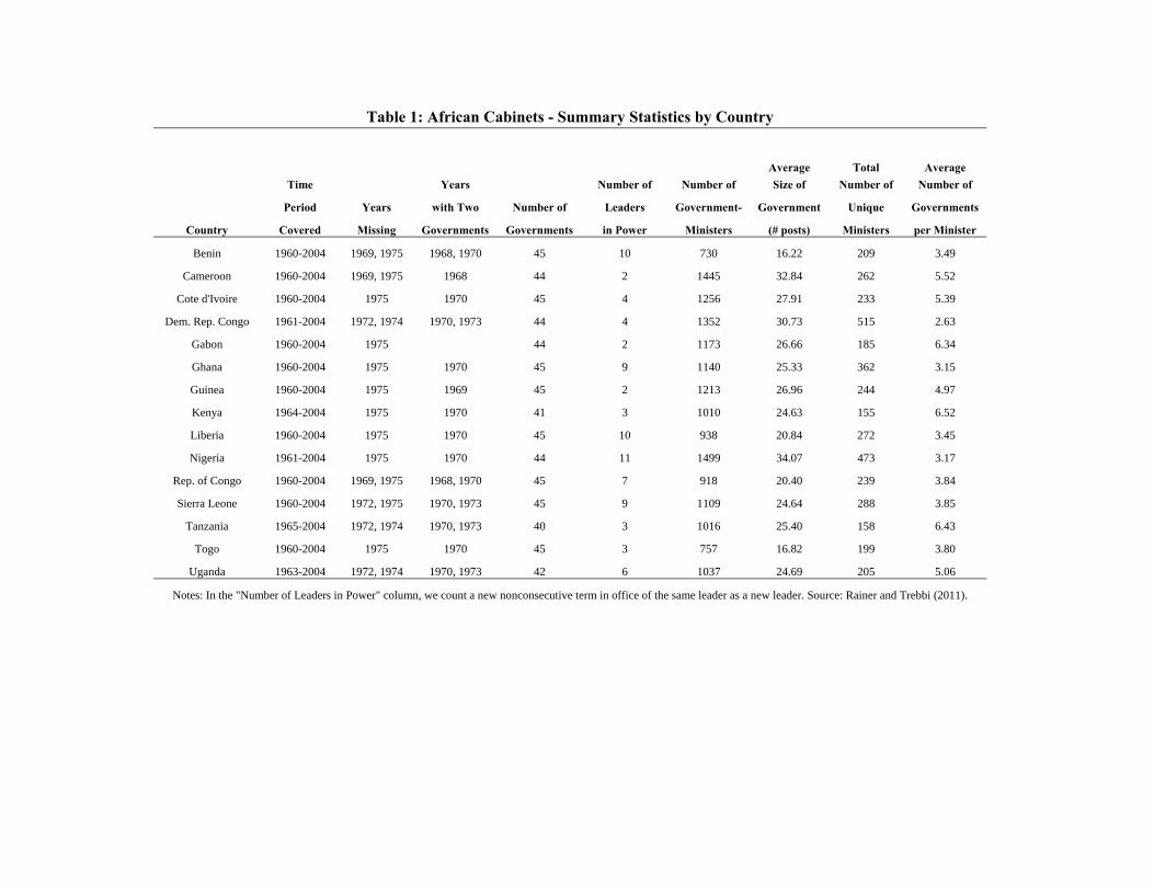
Table 1: African Cabinets - Summary Statistics by Country

Average Total Average Time Years Number of Number of Size of Number of Number of

Period Years with Two Number of Leaders Government- Government Unique Governments

Country Covered Missing Governments Governments in Power Ministers (# posts) Ministers per Minister

Benin 1960-2004 1969, 1975 1968, 1970 45 10 730 16.22 209 3.49

Cameroon 1960-2004 1969, 1975 1968 44 2 1445 32.84 262 5.52

Cote d'Ivoire 1960-2004 1975 1970 45 4 1256 27.91 233 5.39

Dem. Rep. Congo 1961-2004 1972, 1974 1970, 1973 44 4 1352 30.73 515 2.63

Gabon 1960-2004 1975 44 2 1173 26.66 185 6.34

Ghana 1960-2004 1975 1970 45 9 1140 25.33 362 3.15

Guinea 1960-2004 1975 1969 45 2 1213 26.96 244 4.97

Kenya 1964-2004 1975 1970 41 3 1010 24.63 155 6.52

Liberia 1960-2004 1975 1970 45 10 938 20.84 272 3.45

Nigeria 1961-2004 1975 1970 44 11 1499 34.07 473 3.17

Rep. of Congo 1960-2004 1969, 1975 1968, 1970 45 7 918 20.40 239 3.84

Sierra Leone 1960-2004 1972, 1975 1970, 1973 45 9 1109 24.64 288 3.85

Tanzania 1965-2004 1972, 1974 1970, 1973 40 3 1016 25.40 158 6.43

Togo 1960-2004 1975 1970 45 3 757 16.82 199 3.80

Uganda 1963-2004 1972, 1974 1970, 1973 42 6 1037 24.69 205 5.06

Notes: In the "Number of Leaders in Power" column, we count a new nonconsecutive term in office of the same leader as a new leader. Source: Rainer and Trebbi (2011).  

 

 

 

 

 

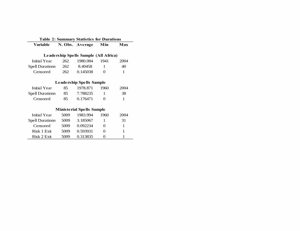
Variable N. Obs. Average Min Max

Initial Year 262 1980.084 1941 2004Spell Durationn 262 8.40458 1 40

Censored 262 0.145038 0 1

Initial Year 85 1978.871 1960 2004Spell Durationn 85 7.788235 1 38

Censored 85 0.176471 0 1

Initial Year 5009 1983.994 1960 2004Spell Durationn 5009 3.185067 1 31

Censored 5009 0.092234 0 1Risk 1 Exit 5009 0.593931 0 1Risk 2 Exit 5009 0.313835 0 1

Ministerial Spells Sample

Leadership Spells Sample

Leadership Spells Sample (All Africa)

Table 2: Summary Statistics for Durations

 

 

 

 

 

 

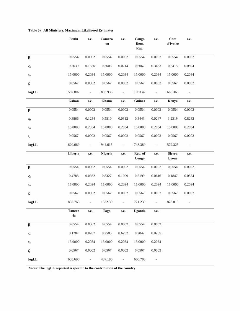
Table 3a: All Ministers. Maximum Likelihood Estimates

Benin s.e. Camero-on

s.e. Congo Dem. Rep.

s.e. Cote d'Ivoire

s.e.

0.0554 0.0002 0.0554 0.0002 0.0554 0.0002 0.0554 0.0002

ςc 0.5639 0.1356 0.3603 0.0214 0.6062 0.3463 0.5415 0.0894

tδ 15.0000 0.2034 15.0000 0.2034 15.0000 0.2034 15.0000 0.2034

0.0567 0.0002 0.0567 0.0002 0.0567 0.0002 0.0567 0.0002

logLL 587.807 - 803.936 - 1063.42 - 665.365 -

Gabon s.e. Ghana s.e. Guinea s.e. Kenya s.e.

0.0554 0.0002 0.0554 0.0002 0.0554 0.0002 0.0554 0.0002

ςc 0.3866 0.1234 0.5510 0.0812 0.3443 0.0247 1.2319 0.8232

tδ 15.0000 0.2034 15.0000 0.2034 15.0000 0.2034 15.0000 0.2034

0.0567 0.0002 0.0567 0.0002 0.0567 0.0002 0.0567 0.0002

logLL 620.669 - 944.615 - 748.389 - 579.325 -

Liberia s.e. Nigeria s.e. Rep. of Congo

s.e. Sierra Leone

s.e.

0.0554 0.0002 0.0554 0.0002 0.0554 0.0002 0.0554 0.0002

ςc 0.4788 0.0362 0.8327 0.1009 0.5199 0.0616 0.1847 0.0554

tδ 15.0000 0.2034 15.0000 0.2034 15.0000 0.2034 15.0000 0.2034

0.0567 0.0002 0.0567 0.0002 0.0567 0.0002 0.0567 0.0002

logLL 832.763 - 1332.30 - 721.239 - 878.019 -

Tanzan-ia

s.e. Togo s.e. Uganda s.e.

0.0554 0.0002 0.0554 0.0002 0.0554 0.0002

ςc 0.1787 0.0207 0.2583 0.6292 0.2842 0.0265

tδ 15.0000 0.2034 15.0000 0.2034 15.0000 0.2034

0.0567 0.0002 0.0567 0.0002 0.0567 0.0002

logLL 603.696 - 487.196 - 660.708 -

Notes: The logLL reported is specific to the contribution of the country.

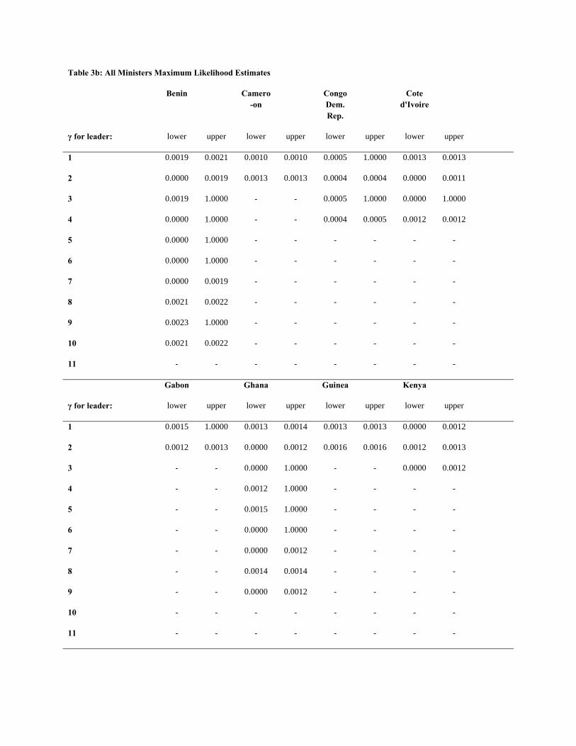
Table 3b: All Ministers Maximum Likelihood Estimates

Benin Camero-on

Congo Dem. Rep.

Cote d'Ivoire

γ for leader: lower upper lower upper lower upper lower upper

1 0.0019 0.0021 0.0010 0.0010 0.0005 1.0000 0.0013 0.0013

2 0.0000 0.0019 0.0013 0.0013 0.0004 0.0004 0.0000 0.0011

3 0.0019 1.0000 - - 0.0005 1.0000 0.0000 1.0000

4 0.0000 1.0000 - - 0.0004 0.0005 0.0012 0.0012

5 0.0000 1.0000 - - - - - -

6 0.0000 1.0000 - - - - - -

7 0.0000 0.0019 - - - - - -

8 0.0021 0.0022 - - - - - -

9 0.0023 1.0000 - - - - - -

10 0.0021 0.0022 - - - - - -

11 - - - - - - - -

Gabon Ghana Guinea Kenya

γ for leader: lower upper lower upper lower upper lower upper

1 0.0015 1.0000 0.0013 0.0014 0.0013 0.0013 0.0000 0.0012

2 0.0012 0.0013 0.0000 0.0012 0.0016 0.0016 0.0012 0.0013

3 - - 0.0000 1.0000 - - 0.0000 0.0012

4 - - 0.0012 1.0000 - - - -

5 - - 0.0015 1.0000 - - - -

6 - - 0.0000 1.0000 - - - -

7 - - 0.0000 0.0012 - - - -

8 - - 0.0014 0.0014 - - - -

9 - - 0.0000 0.0012 - - - -

10 - - - - - - - -

11 - - - - - - - -

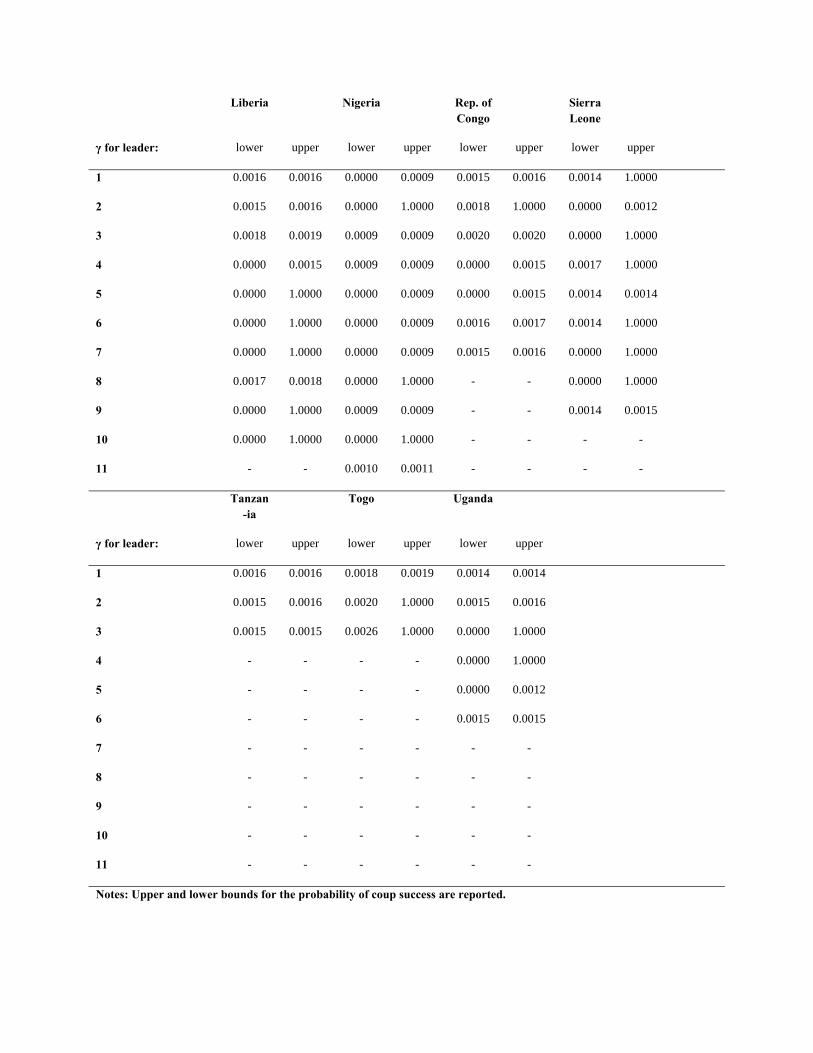
Liberia Nigeria Rep. of Congo

Sierra Leone

γ for leader: lower upper lower upper lower upper lower upper

1 0.0016 0.0016 0.0000 0.0009 0.0015 0.0016 0.0014 1.0000

2 0.0015 0.0016 0.0000 1.0000 0.0018 1.0000 0.0000 0.0012

3 0.0018 0.0019 0.0009 0.0009 0.0020 0.0020 0.0000 1.0000

4 0.0000 0.0015 0.0009 0.0009 0.0000 0.0015 0.0017 1.0000

5 0.0000 1.0000 0.0000 0.0009 0.0000 0.0015 0.0014 0.0014

6 0.0000 1.0000 0.0000 0.0009 0.0016 0.0017 0.0014 1.0000

7 0.0000 1.0000 0.0000 0.0009 0.0015 0.0016 0.0000 1.0000

8 0.0017 0.0018 0.0000 1.0000 - - 0.0000 1.0000

9 0.0000 1.0000 0.0009 0.0009 - - 0.0014 0.0015

10 0.0000 1.0000 0.0000 1.0000 - - - -

11 - - 0.0010 0.0011 - - - -

Tanzan-ia

Togo Uganda

γ for leader: lower upper lower upper lower upper

1 0.0016 0.0016 0.0018 0.0019 0.0014 0.0014

2 0.0015 0.0016 0.0020 1.0000 0.0015 0.0016

3 0.0015 0.0015 0.0026 1.0000 0.0000 1.0000

4 - - - - 0.0000 1.0000

5 - - - - 0.0000 0.0012

6 - - - - 0.0015 0.0015

7 - - - - - -

8 - - - - - -

9 - - - - - -

10 - - - - - -

11 - - - - - -

Notes: Upper and lower bounds for the probability of coup success are reported.

 

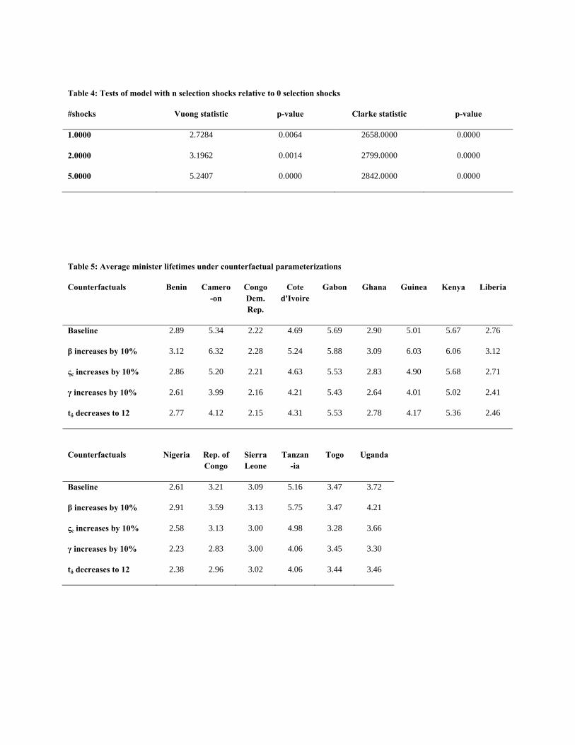
Table 4: Tests of model with n selection shocks relative to 0 selection shocks

#shocks Vuong statistic p-value Clarke statistic p-value

1.0000 2.7284 0.0064 2658.0000 0.0000

2.0000 3.1962 0.0014 2799.0000 0.0000

5.0000 5.2407 0.0000 2842.0000 0.0000

Table 5: Average minister lifetimes under counterfactual parameterizations

Counterfactuals Benin Camero-on

Congo Dem. Rep.

Cote d'Ivoire

Gabon Ghana Guinea Kenya Liberia

Baseline 2.89 5.34 2.22 4.69 5.69 2.90 5.01 5.67 2.76

β increases by 10% 3.12 6.32 2.28 5.24 5.88 3.09 6.03 6.06 3.12

ςc increases by 10% 2.86 5.20 2.21 4.63 5.53 2.83 4.90 5.68 2.71

γ increases by 10% 2.61 3.99 2.16 4.21 5.43 2.64 4.01 5.02 2.41

tδ decreases to 12 2.77 4.12 2.15 4.31 5.53 2.78 4.17 5.36 2.46

Counterfactuals Nigeria Rep. of Congo

Sierra Leone

Tanzan-ia

Togo Uganda

Baseline 2.61 3.21 3.09 5.16 3.47 3.72

β increases by 10% 2.91 3.59 3.13 5.75 3.47 4.21

ςc increases by 10% 2.58 3.13 3.00 4.98 3.28 3.66

γ increases by 10% 2.23 2.83 3.00 4.06 3.45 3.30

tδ decreases to 12 2.38 2.96 3.02 4.06 3.44 3.46

 

Table 6: Output losses

Benin Camero-on

Congo Dem. Rep.

Cote d'Ivoire

Gabon Ghana Guinea Kenya Liberia

Percentage 25.6 48.8 35.8 16.8 80.5 19.3 46.3 53.1 36.0

Nigeria Rep. of Congo

Sierra Leone

Tanzan-ia

Togo Uganda

Percentage 27.4 42.3 33.1 36.8 72.9 31.3

Notes: Actual output as a percentage of counterfactual output levels under the most productive cabinet observed in the country over period 1960-2004 are reported.

 

   

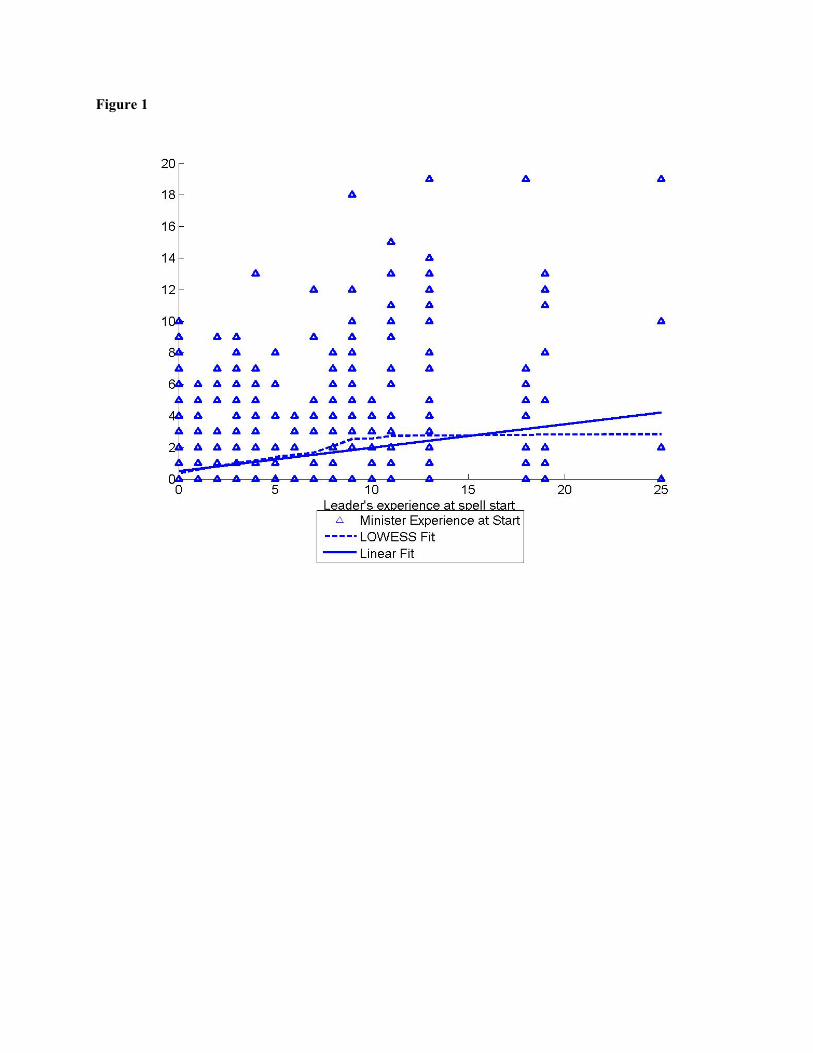
Figure 1

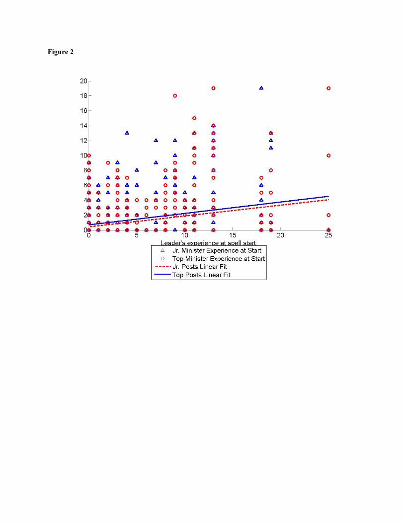
Figure 2

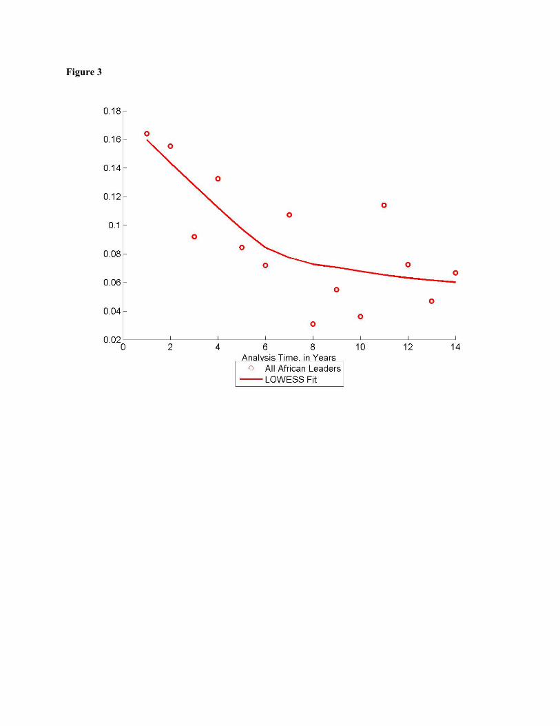
Figure 3

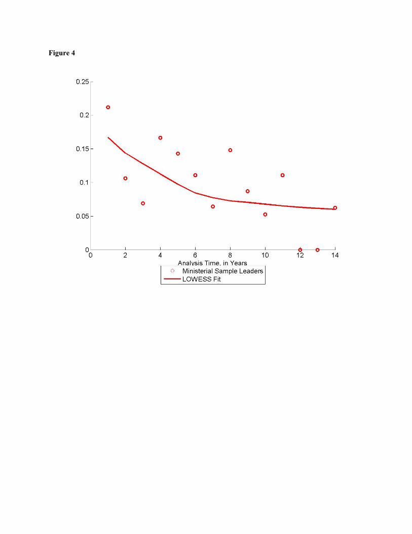
Figure 4

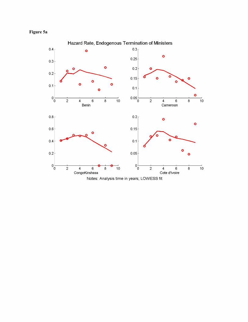
Figure 5a

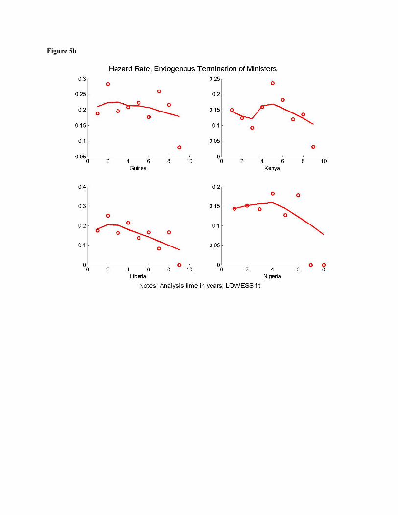
Figure 5b

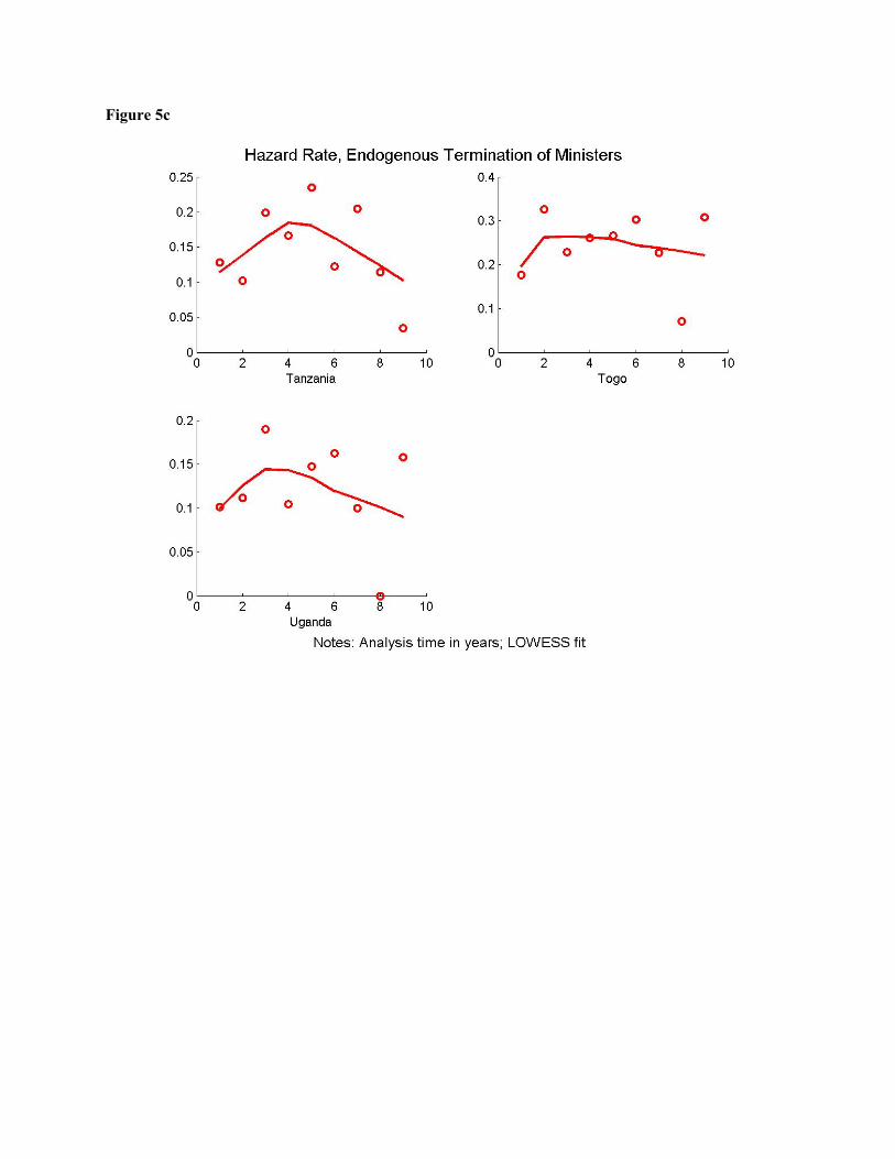
Figure 5c

Figure 5d

Figure 6: Timing

t t+1 t-1 Draw ci(t) Draw ci(t+1)

Exogenous termination draws

Coup decision if coup capacity is met

Hold up opportunity & Bargaining over surplus

Leader decides terminations & Replacements

Production occurs & Consumption shares allocated

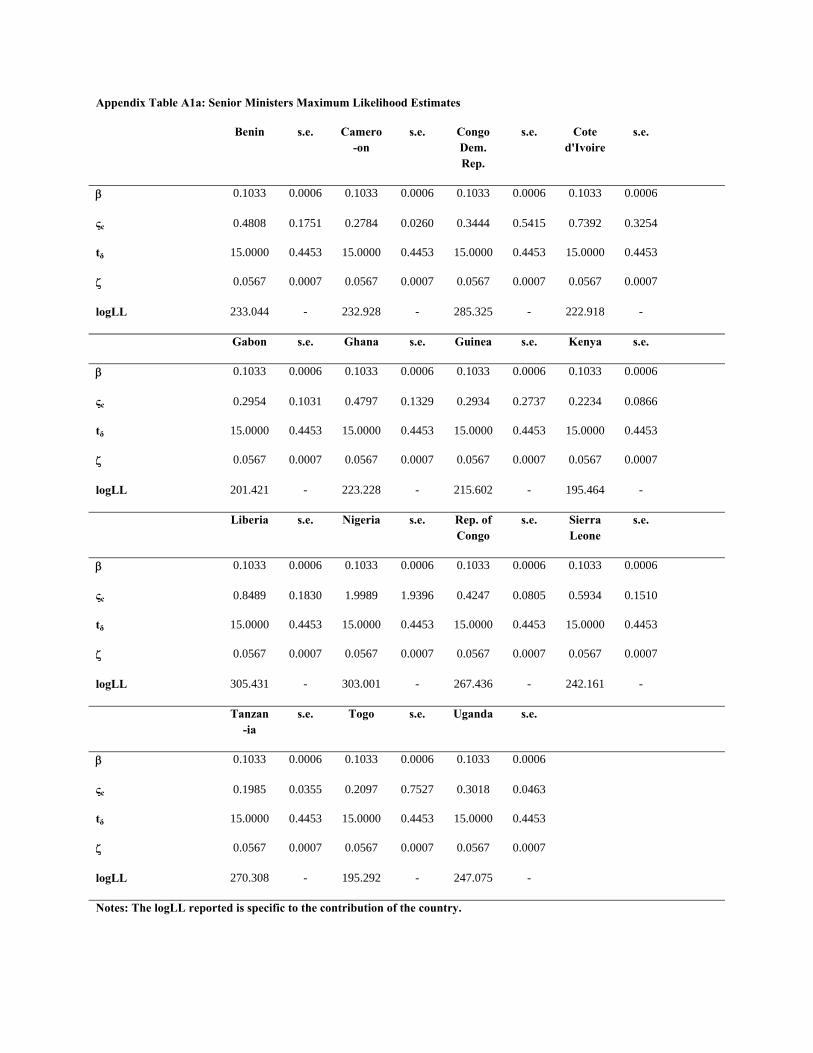
Appendix Table A1a: Senior Ministers Maximum Likelihood Estimates

Benin s.e. Camero-on

s.e. CongoDem. Rep.

s.e. Cote d'Ivoire

s.e.

0.1033 0.0006 0.1033 0.0006 0.1033 0.0006 0.1033 0.0006

ςc 0.4808 0.1751 0.2784 0.0260 0.3444 0.5415 0.7392 0.3254

tδ 15.0000 0.4453 15.0000 0.4453 15.0000 0.4453 15.0000 0.4453

0.0567 0.0007 0.0567 0.0007 0.0567 0.0007 0.0567 0.0007

logLL 233.044 - 232.928 - 285.325 - 222.918 -

Gabon s.e. Ghana s.e. Guinea s.e. Kenya s.e.

0.1033 0.0006 0.1033 0.0006 0.1033 0.0006 0.1033 0.0006

ςc 0.2954 0.1031 0.4797 0.1329 0.2934 0.2737 0.2234 0.0866

tδ 15.0000 0.4453 15.0000 0.4453 15.0000 0.4453 15.0000 0.4453

0.0567 0.0007 0.0567 0.0007 0.0567 0.0007 0.0567 0.0007

logLL 201.421 - 223.228 - 215.602 - 195.464 -

Liberia s.e. Nigeria s.e. Rep. of Congo

s.e. Sierra Leone

s.e.

0.1033 0.0006 0.1033 0.0006 0.1033 0.0006 0.1033 0.0006

ςc 0.8489 0.1830 1.9989 1.9396 0.4247 0.0805 0.5934 0.1510

tδ 15.0000 0.4453 15.0000 0.4453 15.0000 0.4453 15.0000 0.4453

0.0567 0.0007 0.0567 0.0007 0.0567 0.0007 0.0567 0.0007

logLL 305.431 - 303.001 - 267.436 - 242.161 -

Tanzan-ia

s.e. Togo s.e. Uganda s.e.

0.1033 0.0006 0.1033 0.0006 0.1033 0.0006

ςc 0.1985 0.0355 0.2097 0.7527 0.3018 0.0463

tδ 15.0000 0.4453 15.0000 0.4453 15.0000 0.4453

0.0567 0.0007 0.0567 0.0007 0.0567 0.0007

logLL 270.308 - 195.292 - 247.075 -

Notes: The logLL reported is specific to the contribution of the country.

 

Appendix Table A1b: Senior Ministers Maximum Likelihood Estimates

Benin Camero-on

Congo Dem. Rep.

Cote d'Ivoire

γ for leader: lower upper lower upper lower upper lower upper

1 0.0042 0.0044 0.0026 0.0026 0.0010 1.0000 0.0022 0.0023

2 0.0000 0.0039 0.0026 0.0026 0.0011 1.0000 0.0000 0.0022

3 0.0039 1.0000 - - 0.0009 0.0009 0.0000 1.0000

4 0.0000 1.0000 - - 0.0009 0.0009 0.0023 0.0025

5 0.0000 1.0000 - - - - - -

6 0.0000 1.0000 - - - - - -

7 0.0000 0.0039 - - - - - -

8 0.0039 0.0042 - - - - - -

9 0.0046 1.0000 - - - - - -

10 0.0044 0.0046 - - - - - -

11 - - - - - - - -

Gabon Ghana Guinea Kenya

γ for leader: lower upper lower upper lower upper lower upper

1 0.0030 1.0000 0.0026 0.0028 0.0026 0.0027 0.0000 0.0025

2 0.0026 0.0027 0.0026 1.0000 0.0033 1.0000 0.0030 0.0031

3 - - 0.0000 1.0000 - - 0.0000 0.0025

4 - - 0.0025 1.0000 - - - -

5 - - 0.0030 0.0031 - - - -

6 - - 0.0000 0.0025 - - - -

7 - - 0.0000 1.0000 - - - -

8 - - 0.0000 0.0025 - - - -

9 - - - - - - - -

10 - - - - - - - -

11 - - - - - - - -

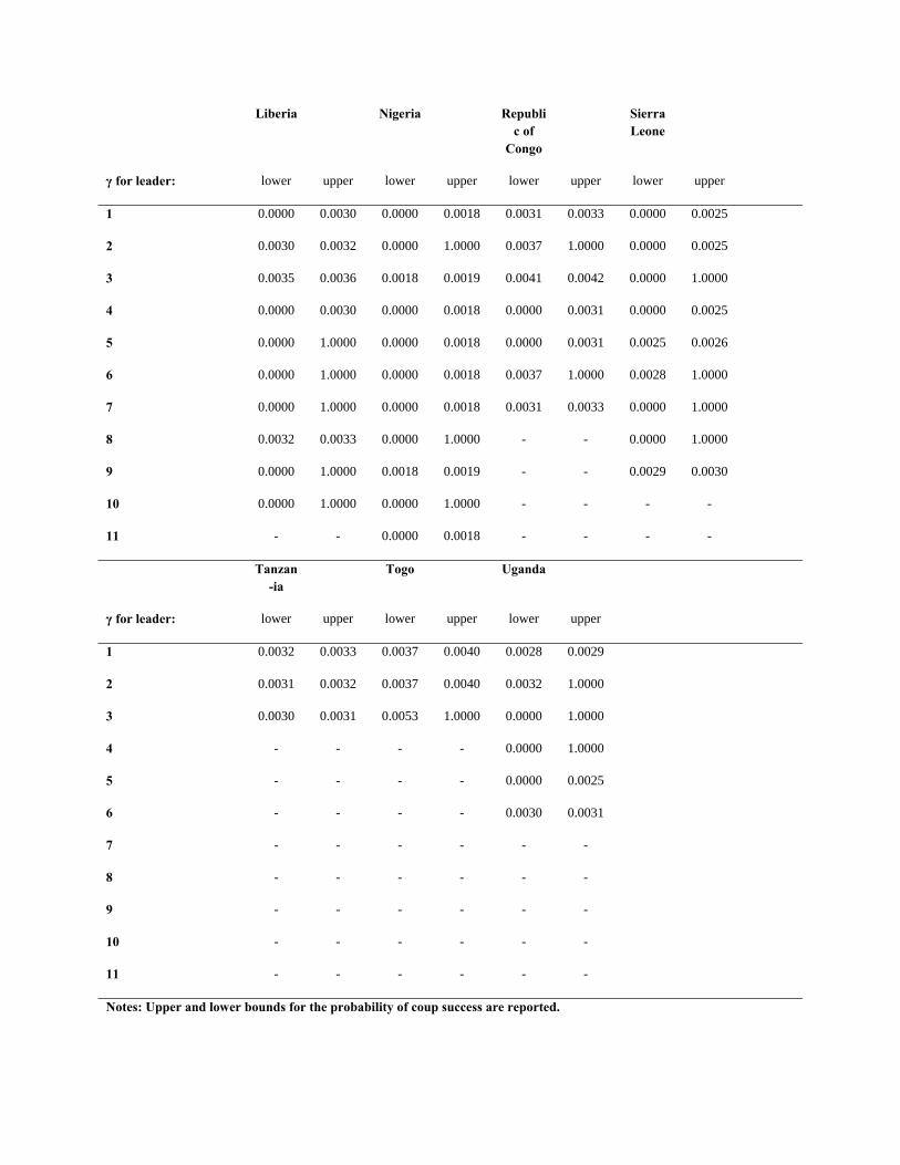
Liberia Nigeria Republic of

Congo

Sierra Leone

γ for leader: lower upper lower upper lower upper lower upper

1 0.0000 0.0030 0.0000 0.0018 0.0031 0.0033 0.0000 0.0025

2 0.0030 0.0032 0.0000 1.0000 0.0037 1.0000 0.0000 0.0025

3 0.0035 0.0036 0.0018 0.0019 0.0041 0.0042 0.0000 1.0000

4 0.0000 0.0030 0.0000 0.0018 0.0000 0.0031 0.0000 0.0025

5 0.0000 1.0000 0.0000 0.0018 0.0000 0.0031 0.0025 0.0026

6 0.0000 1.0000 0.0000 0.0018 0.0037 1.0000 0.0028 1.0000

7 0.0000 1.0000 0.0000 0.0018 0.0031 0.0033 0.0000 1.0000

8 0.0032 0.0033 0.0000 1.0000 - - 0.0000 1.0000

9 0.0000 1.0000 0.0018 0.0019 - - 0.0029 0.0030

10 0.0000 1.0000 0.0000 1.0000 - - - -

11 - - 0.0000 0.0018 - - - -

Tanzan-ia

Togo Uganda

γ for leader: lower upper lower upper lower upper

1 0.0032 0.0033 0.0037 0.0040 0.0028 0.0029

2 0.0031 0.0032 0.0037 0.0040 0.0032 1.0000

3 0.0030 0.0031 0.0053 1.0000 0.0000 1.0000

4 - - - - 0.0000 1.0000

5 - - - - 0.0000 0.0025

6 - - - - 0.0030 0.0031

7 - - - - - -

8 - - - - - -

9 - - - - - -

10 - - - - - -

11 - - - - - -

Notes: Upper and lower bounds for the probability of coup success are reported.

   

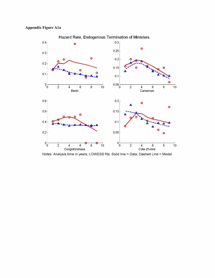
Appendix Figure A1a

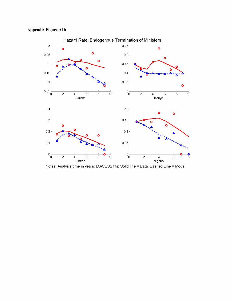
Appendix Figure A1b

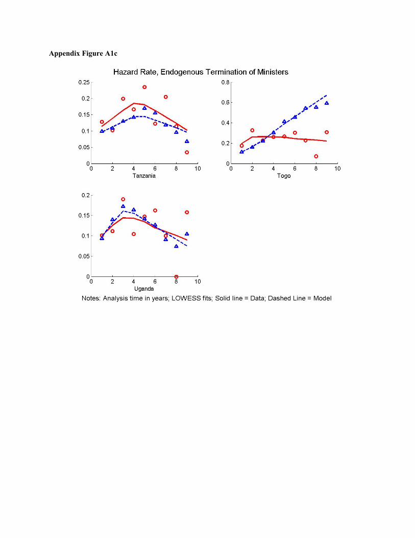
Appendix Figure A1c

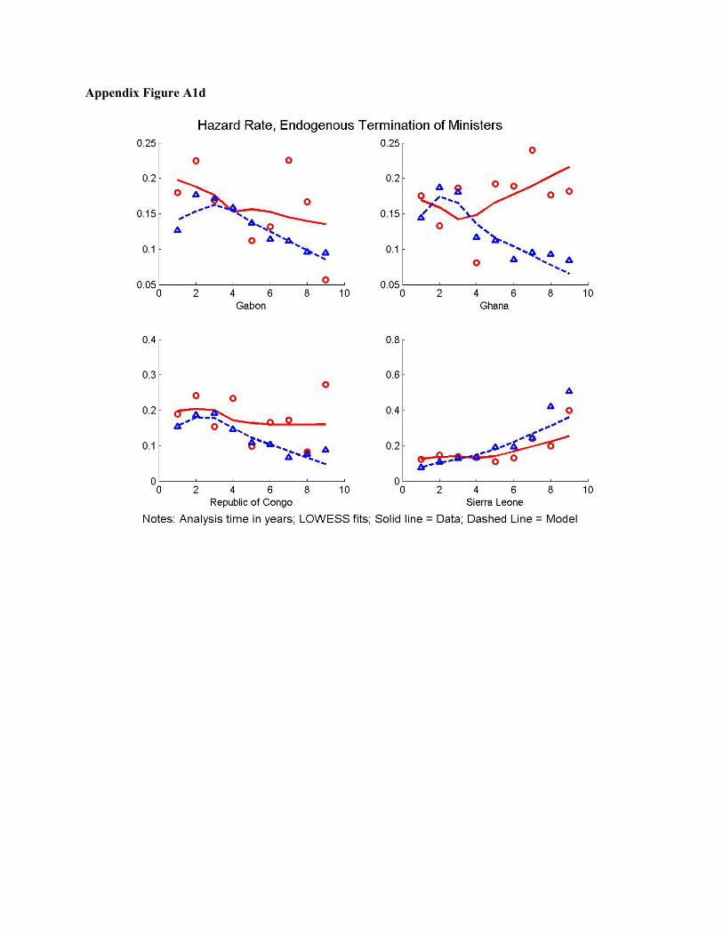
Appendix Figure A1d

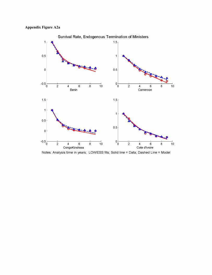
Appendix Figure A2a

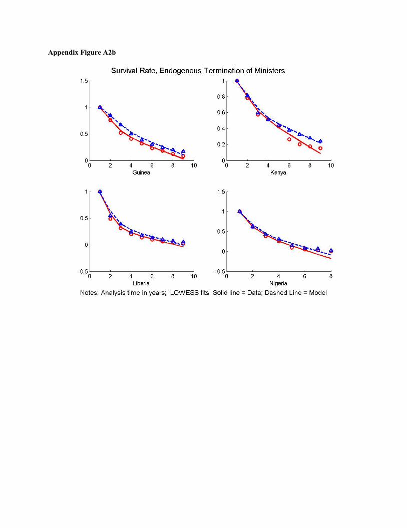
Appendix Figure A2b

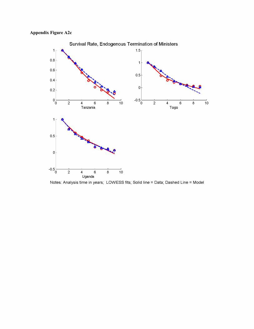
Appendix Figure A2c

Appendix Figure A2d