AIRCRAFT MODELLING AND PERFORMANCE PREDICTION SOFTWARE IN A SIMULATED ENVIRONMENT

KEY ASPECTS

Day 1

Document search Jane’s Information

Wikipedia

Type Certificate

Research papers

Pictures

3-View

Technical Manual – Pilot Training Manual

Manufacturers Technical Data sheets

Pilots Operating Handbooks

The Diary of a Beechcraft King Air B200 Aircraft Model Build

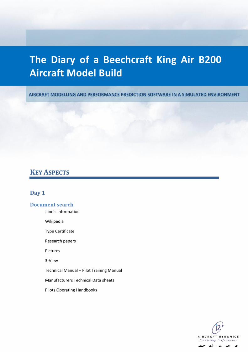
Control Surfaces and Geometry From the document search Identify Airfoil Shapes and control surface types. Flaps are single slotted.

Find a research paper on single slotted flaps for NACA 23012 wind tunnel results. This paper gives

flap, nose profile and slot profile. This can also be used as a reference check.

Inboard Wing and Flaps Coefficient Data Start to use JavaFoil to build aerodynamic coefficient data for the flapped sections. This needs to be

done for all airfoil sections. Run at the appropriate Reynolds number up to a maxim deflection of

40° (Flaps limit is 35°)

Day 2

Wing and Aileron Coefficient Data Wing, Aileron (20%) and Aileron Tab (6%) Coefficient data. Looking at the Tab and the Aileron

together.

All combinations gives the influence of the Aileron for inboard and outboard wing on the

coefficients, the tab was only looked at its limits and then simplified, because the tabbed section is

very small, giving small contributions.

The ailerons only needed to be considered for the 16.5% and 12% thickness sections.

Power Effects on Airplane Lift Study to obtain definitive values. According to Roskam Airplane Design Part VI

∑(

) ( ) (

)

Where

(ft/s)

Dimensional analysis of this to convert to SI gives

∑(

) ( ) (

)

Where

(m/s)

This helps with understanding and removes “magic” numbers such as 2200.

∑(

) ( )(

)

Day 3

Empennage No data exists on the Airfoils for the empennage. It is assumed that the sections will be symmetric

NACA 00XX airfoils. The drawing was used to identify the thickness of the section. These were

estimated to be 10%.

From the drawings, the Elevator was estimated to be 40% and the Elevator Tab, 9% chord.

From the drawings, the Rudder was estimated to be 45% and the Rudder Tab, 8.5% chord

These were run over a range of deflections for HT, Elevator and Elevator Tab, and VT, Rudder and

Rudder Tab.

The primary Surface contributions at zero tab deflections could be used as simple lookup tables.

However, once the tabs were added in, these created an extra dimension to tables. As these were

small contributions, it was decided that the best approach for these would be to find trends at the

extremes of the tab deflection and corresponding main surface deflections (min, 0, and max).

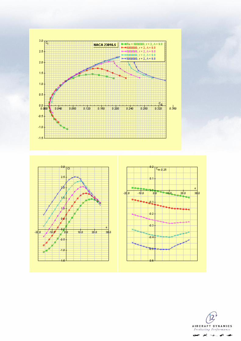
Lift Contribution of Rudder Tab at different angles of VT and Rudder, and Rudder Tab Deflection

Lift and Pitch became simple derivatives of the tab deflection. However for drag, there was an offset

and gradient shift. This meant performing simple linear curve fits to the drag curves.

Drag Contribution of Elevator Tab

From here we can calculate increments in drag due to tab deflection at different primary surface

deflections and then a drag derivative due to alphas a function of tab deflection.

dET -4 0 13

dCd/dAlpha (/°)

-0.0011 0 0.004

dCd

dET

-4 0 13

dE

-25 0.0197 0 -0.0532

0 0.0004 0 0.0077

15 -0.0122 0 0.0543

Day 4

Fuselage The idea with the fuselage was to extract the data from DATCOM analysis. A similar approach can

be performed using Roskam. Most fuselage approaches require the construction of the fuselage

geometry to identify key features. To do this the 3-View was used, with dimensions measured

directly from the drawing.

DATCOM can only give results with Elliptical Fuselage.

Model Assembly Once the fuselage has been built, the next stage is to start to assemble the model. Initially the basic

structure, components and reference information was added as well as the geometry for the

stripped items. Downwash calculations are added.

Wing Aerodynamics Start to assemble the wing characteristics. Total Wing Contributions are made up of 3 sections

Clean wing varying with Angle of Attack and Spanwise position to take account of the different airfoil

sections

Flaps contribution, 3-D lookup tables with an increment due to flap deflections of range of angle of

attack and spanwise position

Aileron contributions – separated out into left and right, 3-D lookup tables giving increments due to

aileron deflection varying with angle of attack and spanwise position but only considering the

outboard section of the wing.

The last control surface to be added is a small aileron tabbed section to include the increments due

to the aileron tab.

Day 5

Propwash Add in the power into the model. Expose the Lift Coefficient for the Clean Wing and increment due

to flaps.

Create Left and Right Propwash Stripped Items. Using the formulae found previously, add the

propwash contributions

Fuselage Add in the coefficients found for the fuselage

Empennage Add in the coefficient data for the Vertical Tail and Rudder, and then additional contribution due to

tab.

Add in the coefficient data for the Horizontal Tail and Elevator, and then additional contribution due

to tab.

Mass Information Mass and inertia are supplied in the flight test information, so initially, these values will be used.

Eventually, calculations will be added to more accurately model the mass information.

Initial Build Complete

Initial Analysis Working with the test cases supplied, take a first look at what errors are present. This is almost a

whim just to see how good the initial model is. Initially there is no propwash. Add power to trim

scenarios and manoeuvres to include the propwash.

Initial quick investigations identified a little too much tail authority and lift. Reduce lift on wing by

taking out the fuselage section. This is already covered with fuselage lift.

Similar approach to pitch surfaces when looking in more detail at the tail.

Initial evaluation against a single flight test case enabled reasonable results.

Day 6 After the initial tests on flight test data, it was decided to go back to some of the basic principles to

evaluate the model following a better process.

Longitudinal Sanity Checks Run alpha sweep at different elevator deflections and different flap deflections to get some idea as

to the total values for the aircraft. The lift from the wing can be used to correct alpha equivalent

values by using the correct lift curve slope.

The Lift from the wing can be used to give Cla for calculation of equivalent Alpha.

Total Cla for the aircraft is 6.24/rad when compared to similar aircraft from Roskam we have a total

lift curve value of approx. 5.5 so we can reduce the lift on the wing to account for this.

The CMa is -4.8 which is much larger than that for a similar class of aircraft. This is mainly due to the

lift from the tail, so can be reduced by changing the lift curve slope on the tail.

The Cmde and Clde values are -4.1 and 0.89 respectively. Again when comparing to Roskam these

are higher than expected. In this scenario therefore we can reduce the Lift contribution of the

Elevator, which will have a corresponding effect on the Pitch.

Finally we can look at the downwash values and compare these to those found running the basic

DatCom analysis. These are similar values, bearing in mind that DatCom does not use the Equivalent

Alpha approach.

These values give ideas for certain corrections that will be put into the baseline model.

Simple Static Analysis Once some simple corrections have been added, we can start to look at the steady state

characteristics for flights. We can look at the simple balance for the Lift and Pitch at the beginning of

a flight. For steady state, we know that mg/dynamic.S = CL and Cm=0. So

Mg/dynamic.S=CLt

Clt = CLo + CL.+ CLat +CLe e +CLet et

0 = Cmo- CLt sm => 0=Cmo - sm. Mg/dynamic.S

If we assume lift curve slopes to be correct, this leaves us with 3 unknowns. The static margin (sm)

will be dependent upon the lift distribution between the Wing and Tail

Cmo, CLo,

We can initialise the aircraft at the desired condition and then run a range of alpha sweeps to

identify the static margin and to see how small changes to the model impact the desired condition.

The only flight data that is available with no flaps is case 5B

H=7938ft

CAS = 157kts

M= 11947ln

= 3.1°

e = 0.5°

et = 1.3°

CG = 21.9%

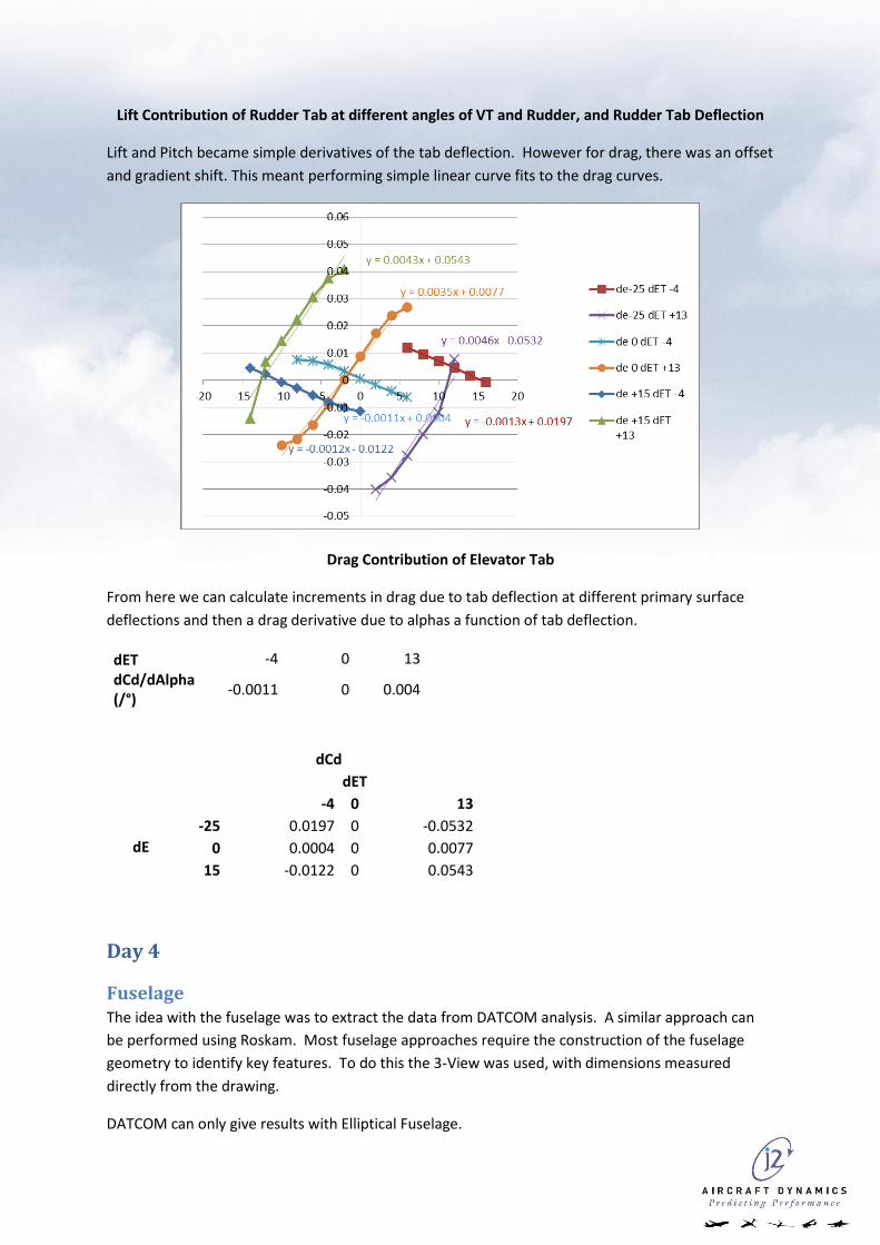
These analyses will be initially performed on a delta model to identify corrections for this one case.

If these are found to be suitable for all cases they can be put into the baseline model. Changes to

Cmo, CLo, and downwash will be investigated to see how each can impact the design. To effect the

downwash, the tail incidence was changed to represent an increased value. Changes to Cmo and

CLo for study purposes were placed at the 25% mac of the wing as global values.

From the above chart, we can see that the change in the downwash had a slight change in the static

margin, but the other changes were unnoticeable.

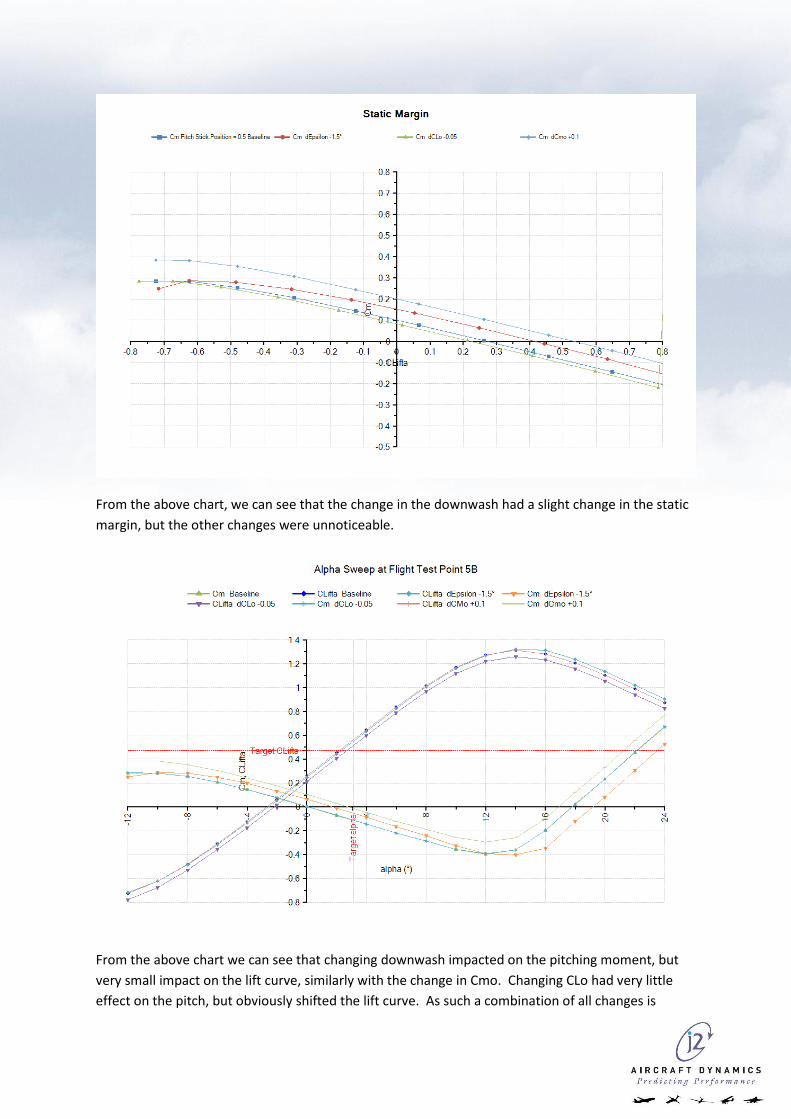
From the above chart we can see that changing downwash impacted on the pitching moment, but

very small impact on the lift curve, similarly with the change in Cmo. Changing CLo had very little

effect on the pitch, but obviously shifted the lift curve. As such a combination of all changes is

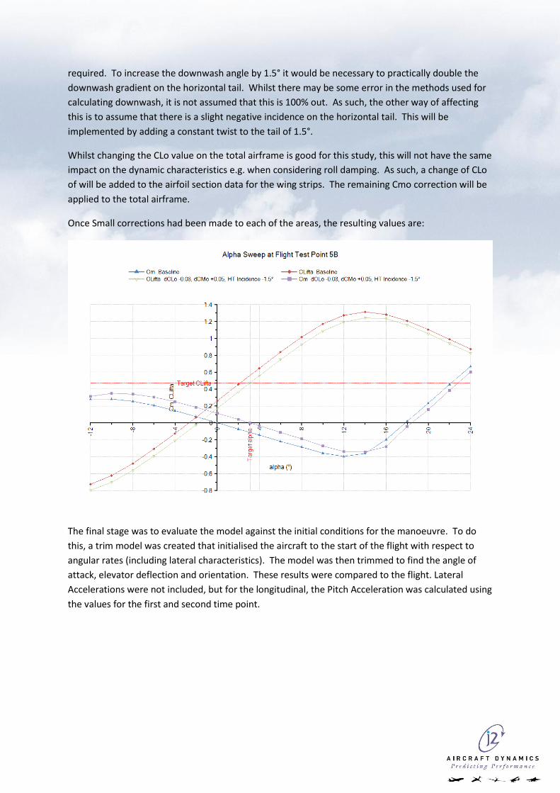
required. To increase the downwash angle by 1.5° it would be necessary to practically double the

downwash gradient on the horizontal tail. Whilst there may be some error in the methods used for

calculating downwash, it is not assumed that this is 100% out. As such, the other way of affecting

this is to assume that there is a slight negative incidence on the horizontal tail. This will be

implemented by adding a constant twist to the tail of 1.5°.

Whilst changing the CLo value on the total airframe is good for this study, this will not have the same

impact on the dynamic characteristics e.g. when considering roll damping. As such, a change of CLo

of will be added to the airfoil section data for the wing strips. The remaining Cmo correction will be

applied to the total airframe.

Once Small corrections had been made to each of the areas, the resulting values are:

The final stage was to evaluate the model against the initial conditions for the manoeuvre. To do

this, a trim model was created that initialised the aircraft to the start of the flight with respect to

angular rates (including lateral characteristics). The model was then trimmed to find the angle of

attack, elevator deflection and orientation. These results were compared to the flight. Lateral

Accelerations were not included, but for the longitudinal, the Pitch Acceleration was calculated using

the values for the first and second time point.

Tri

m R

ule

Pa

ram

ete

rP

ara

me

ter

% E

rr%

Err

Alp

ha

Tri

mW

'W

'0

g1.0

751E

-16

g0.0

0%

-1.4

147E

-16

g0.0

0%

0.0

0%

ALP

HA

TR

UE

3.0

714

°°

2.3

505

°-2

3.4

7%

3.0

446

°-0

.87%

29.5

3%

Pit

ch

Ra

teQ

'°/

s2

Q'

0°/

s2

-2°/

s2

0.0

0%

-0.3

9°/

s2

0.0

0%

-80.5

0%

ELE

VA

TO

R D

EF

0.4

77409

°°

-1.7

943

°-4

75.8

4%

0.4

467

°-6

.43%

-124.9

0%

La

tera

l S

urf

ace

sP

'°/

s2

P'

0°/

s2

-6.1

363E

-14

°/s

20.0

0%

-5.0

04E

-14

°/s

20.0

0%

0.0

0%

R'

°/s

2R

'0

°/s

2-6

.9648E

-15

°/s

20.0

0%

2.4

841E

-15

°/s

20.0

0%

0.0

0%

AV

G A

IL D

EF

1.2

4921

°°

-0.2

8345

°-1

22.6

9%

-0.2

8435

°-1

22.7

6%

0.3

2%

RU

DD

ER

DE

F

2.3

2074

°°

0.2

867

°-8

7.6

5%

0.2

893

°-8

7.5

3%

0.9

1%

Alt

itu

de

Fix

ed

ALTIT

UD

E7936.8

9ft

ALTIT

UD

E7936.8

9ft

7936

ft-0

.01%

7936

ft-0

.01%

0.0

0%

Ve

locit

y F

ixe

dTA

S181.1

66

kt

TA

S181.1

66

kt

181.2

1kt

0.0

2%

181.2

1kt

0.0

2%

0.0

0%

Se

a L

eve

l T

em

p F

ixe

dS

L T

EM

P301.6

2°K

SL T

EM

P301.6

2°K

301.6

°K-0

.01%

301.6

°K-0

.01%

0.0

0%

AM

BIE

NT

TE

MP

285.9

67

°K°K

285.8

8°K

-0.0

3%

285.8

8°K

-0.0

3%

0.0

0%

Ba

nk i

nto

Win

dV

'g

V'

0g

0.0

11

g0.0

0%

0.0

11

g0.0

0%

0.0

0%

HE

AD

ING

180.8

57

°H

EA

DIN

G

180.8

57

°180.9

°0.0

2%

180.9

°0.0

2%

0.0

0%

BE

TA

TR

UE

-0

.0228

°°

0°

-100.0

0%

0°

-100.0

0%

0.0

0%

RO

LL A

TT

-0

.171381

°°

-0.3

181

°85.6

1%

-0.3

399

°98.3

3%

6.8

5%

Ma

ss T

rim

IZZ

27099.1

slg

-ft

2IZ

Z27099.1

slg

-ft

227099.1

slg

-ft

20.0

0%

27099.1

slg

-ft

20.0

0%

0.0

0%

WE

IGH

T

11946.8

lbW

EIG

HT

11946.8

lb11946.8

lb0.0

0%

11946.8

lb0.0

0%

0.0

0%

IXX

17711.1

slg

-ft

2IX

X17711.1

slg

-ft

217711.1

slg

-ft

20.0

0%

17711.1

slg

-ft

20.0

0%

0.0

0%

IXZ

1146.7

7slg

-ft

2IX

Z1146.7

7slg

-ft

21146.8

slg

-ft

20.0

0%

1146.8

slg

-ft

20.0

0%

0.0

0%

IYY

11127.5

slg

-ft^

2IY

Y11127.5

slg

-ft^

211127.6

slg

-ft

20.0

0%

11127.6

slg

-ft

20.0

0%

0.0

0%

Tri

m C

on

fig

FLA

P D

EF

-0

.5079

°F

LA

P D

EF

-0

.5079

°-0

.5079

°0.0

0%

-0.5

079

°0.0

0%

0.0

0%

GE

AR

0G

EA

R0

00.0

0%

00.0

0%

0.0

0%

STA

TIC

MA

RG

IN21.9

476

%C

G21.9

476

%21.9

4%

-0.0

3%

21.9

4%

-0.0

3%

0.0

0%

Tri

m T

ab

sE

LE

VA

TO

R T

AB

1.2

6619

°E

LE

VA

TO

R T

AB

1.2

6619

°1.2

7°

0.3

0%

1.2

7°

0.3

0%

0.0

0%

AIL

ER

ON

TA

B

1.2

2297

°A

ILE

RO

N T

AB

1.2

2297

°1.2

2°

-0.2

4%

1.2

2°

-0.2

4%

0.0

0%

RU

DD

ER

TA

B

-1.6

3167

°R

UD

DE

R T

AB

-1

.63167

°-1

.63

°-0

.10%

-1.6

3°

-0.1

0%

0.0

0%

En

gin

e F

ixe

dF

NP

-L

2260.3

14883

NF

NP

-L

2260.3

14883

N2260.3

N0.0

0%

2260.3

N0.0

0%

0.0

0%

N1 -

R86.0

436

%N

1 -

R86.0

436

%86.0

4%

0.0

0%

86.0

4%

0.0

0%

0.0

0%

N1 -

L85.7

206

%N

1 -

L85.7

206

%85.7

2%

0.0

0%

85.7

2%

0.0

0%

0.0

0%

FN

P -

R2190.9

93798

NF

NP

-R

2190.9

93798

N2191

N0.0

0%

2191

N0.0

0%

0.0

0%

FN

J -L

89.2

6468726

NF

NJ

-L89.2

6468726

N89.2

6N

-0.0

1%

89.2

6N

-0.0

1%

0.0

0%

Pro

p L

eve

r -R

1.7

6595

INP

rop L

eve

r -R

1.7

6595

IN1.7

7IN

0.2

3%

1.7

7IN

0.2

3%

0.0

0%

FN

J -R

92.4

1536263

NF

NJ

-R92.4

1536263

N92.4

2N

0.0

1%

92.4

2N

0.0

1%

0.0

0%

Pro

p L

eve

r -L

1.8

5625

INP

rop L

eve

r -L

1.8

5625

IN1.8

6IN

0.2

0%

1.8

6IN

0.2

0%

0.0

0%

Ra

tes

Fix

ed

RO

LL R

ATE

0.1

44035

°/s

RO

LL R

ATE

0.1

1°/

s0.1

44

°/s

-0.0

2%

0.1

44

°/s

-0.0

2%

0.0

0%

PIT

CH

RA

TE

0.1

73439

°/s

PIT

CH

RA

TE

0.0

4°/

s0.1

73

°/s

-0.2

5%

0.1

73

°/s

-0.2

5%

0.0

0%

YA

W R

ATE

-0

.0914

°/s

YA

W R

ATE

-0

.25

°/s

-0.0

91

°/s

-0.4

4%

-0.0

91

°/s

-0.4

4%

0.0

0%

Fli

gh

t P

ath

(theta

-alp

ha)

0.3

4638

°gam

ma

0.3

4638

°0.3

5°

1.0

5%

0.3

5°

1.0

5%

0.0

0%

PIT

CH

AT

T

3.4

1778

°°

2.7

004

°-2

0.9

9%

3.3

945

°-0

.68%

25.7

0%

TR

IM T

HR

US

T0

%%

-1.5

156

%0.0

0%

4.5

474

%0.0

0%

-400.0

4%

Ori

gin

al

Mo

de

lD

elt

a 5

B

Va

lue

Va

lue

Re

sult

s

J2 V

ari

ati

on

Tri

m T

arg

et V

alu

eT

arg

et

Fli

gh

t T

est

Co

nd

itio

n

Day 7

Preliminary Dynamic Investigations Up to this point, all the data that has been entered is static aerodynamic characteristics. However,

because of the nature of the model using aerodynamic strip theory and the geometry of the aircraft,

the initial dynamic characteristics are inherent in the model.

The manoeuvre that is taking place in flight 5B is the deployment of the Flaps. The flight test data

was used to create a response model, where the control surfaces are driven directly from the values

measured in flight test, and the engine characteristics from flight test are used to drive the model.

The Shaft Horsepower (SHP) of the engines is used in the propwash calculations. As we are just

looking at the longitudinal characteristics at this point, a simple controller was added to the

response model to move the ailerons in order to “track” the bank angle.

Initially, the investigation is about whether the basic steady state conditions are acceptable, so we

consider the first 7.5s (before the flaps are deployed). The results can be seen below. Whilst the

intention of the initial study is not to see how quickly a Level4/5 model can be built, the JAR limits

for a 6D model have been included for reference.

We can see from the above plots that the model compares very well to the flight test data during the

steady flight section. There is a slight drift in Pitch angle due to the pitch rate being marginally

higher, but this is still well within the limits.

When we look at the complete flight though the model starts to move outside the limits. The impact

of the flaps has the right effect, but this there is too much lift due to the flaps deployment which

affects pitch rate (although this is still within limits). This leads to a large change in the pitch angle

and results in the airspeed dropping (taking both outside the limits).

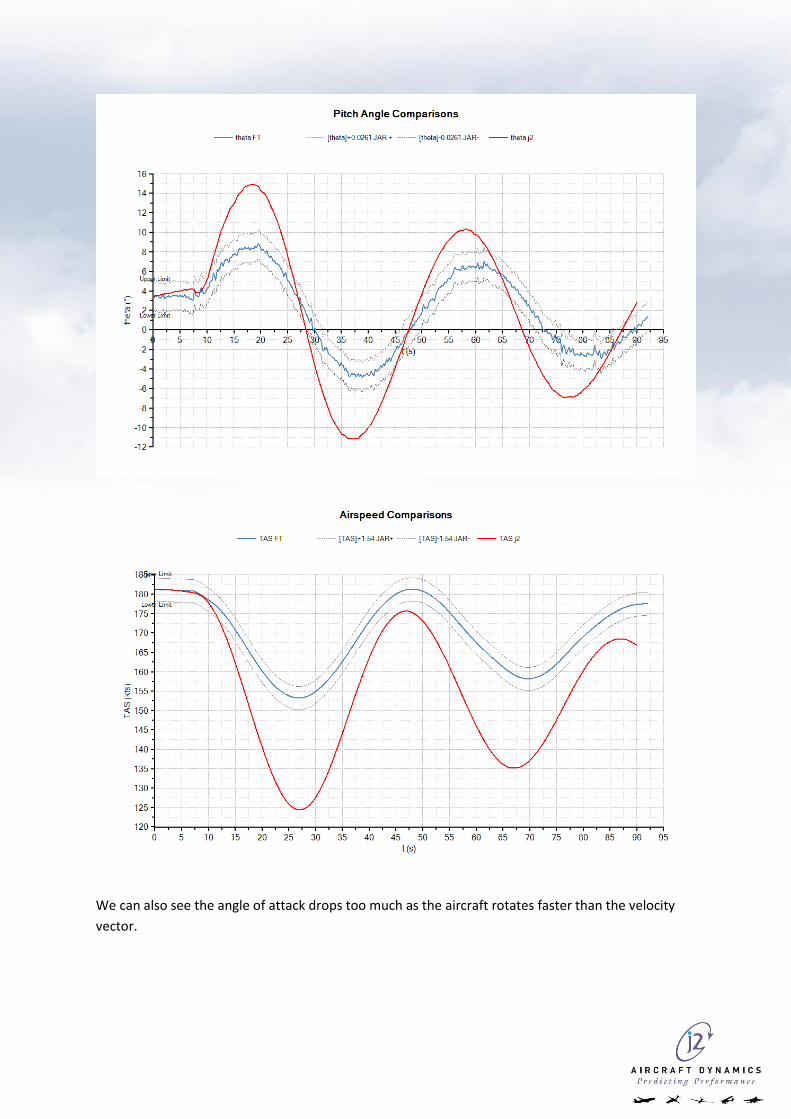
We can also see the angle of attack drops too much as the aircraft rotates faster than the velocity

vector.

The first implication therefore is that the lift due to flaps is too high. Some simple experimentation

at adding an increment to the Lift due to Flaps derivative (-0.01/°) instantly results in a better

comparison.

However, the aircraft is not rotating as fast as the velocity vector, this still results in a reduced angle

of attack.

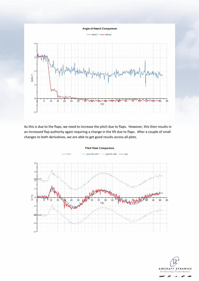
As this is due to the flaps, we need to increase the pitch due to flaps. However, this then results in

an increased flap authority again requiring a change in the lift due to flaps. After a couple of small

changes to both derivatives, we are able to get good results across all plots.

At this point, whilst the results were still not perfect for Level 6D, it was decided that these results

were good enough based on the time taken and the data requirements. Further tweaking or

regression analysis (the subject of an additional paper) could further improve the results but it was

viewed that further test cases should be evaluated before spending any more time on this

manoeuvre. Again it is worth re-iterating that the behaviour of the aircraft has come from the use of

freely available data to build the model, and using the geometry and airfoil characteristics to build a

fully dynamic model.

Day 8

Compare to Other Initial Conditions 4 other flights are available that can be used for validation of the model. In all cases these Flights

start with the flaps extended. Now that the flap characteristics have been tested we can look at the

steady state characteristics of these. Initially we will again start with simple straight and level trim

cases to see if we are getting the correct lift and pitch characteristics.

We will start using the delta model from the previous test.

Flight 6B Flight 5B Flight 5C Flight 6H Flight 6F

Target Results Target Results Target Results Target Results Target Results

Flaps ° 16 15.6 0 -0.5079 15 14.95 13 13.16 14 13.73

Altitude ft 4894 7938 7993 8060 8127

CAS kts 145.8 157.2 146 138.7 123.5

TAS kts 158.23 179.84 167.42 159.61 142.23

Mass lb 11539 11947 10982 12088 11391

cg % 21.3 21.9 20.3 24.6 23.6

° 1.5 0.4144 3.1 3.0141 0.6 0.2812 2 1.7357 3 2.8438

e ° 0.8 1.2961 0.5 0.5233 1.7 1.5377 1.1 0.8153 0.5 -0.7869

et ° 1.8136 1.2662 1.14 1.6099 2.5523

We can see that flights 6B and 6F show the largest discrepancies in alpha and elevator deflection

respectively.

Static Analysis We will start by looking at 6B and 6F, and run a static study into the lift and pitch at the appropriate

Flap and Elevator Settings. As we are happy with the numbers for the 0 Flap setting, we can now

just look at Flap contribution. We build delta models and include the corrections for the un-flapped

condition, but do not add the flap corrections found previously.

Now we can look at the flap contributions and see what changes are required.

Following these two studies and combined with the 5B study, we get corrections of

6B 5B 6F

CL/df -0.037 -0.028 -0.03

Cm/df 0.0105 0.007 0.011

dCL/df -0.009 0 -0.002

dCm/df 0.0045 0 0.004

Note: The 5B values came from quick estimates and experimentation for the dynamic behaviour

whereas the other two came from Steady State Studies. Whilst they are all of a similar order of

magnitude, they are not consistent enough. Ignoring the experimental values, and looking at the

study numbers only, we can see that there is a change in horsepower from 6F to 6B 264 to 345HP so

this could account for the larger lift change required in 6B.

This therefore implies there is a change required for the lift due to propwash. A look up table

derivative was used to correct the lift due to propwash when flaps are deployed.