The development of a laboratory data analysis curriculum for physicsand engineering students.

by

David F. Wong

A THESIS SUBMITTED IN PARTIAL FULFILLMENTOF THE REQUIREMENTS FOR THE DEGREE OF

BACHELOR OF APPLIED SCIENCE.

DIVISION OF ENGINEERING SCIENCE

FACULTY OF APPLIED SCIENCE AND ENGINEERINGUNIVERSITY OF TORONTO

Supervisors: Jason J. B. Harlow and David Bailey

April 2006

i

Abstract

There are notable gaps between formal instruction given to students andthe expectations of students with respect to data analysis. In this work,techniques from physics education research are used to design, implement,and evaluate a curriculum module for data analysis in a third and fourthyear undergraduate physics laboratory. The results of the study includethe deployment of an advanced fitting tool, the establishment of lectureson statistics and data analysis, and a simulated data analysis assignment inwhich students analyze computer generated data with the techniques andtools they are taught. The effectiveness of the module was evaluated usingstatistical analysis from a student survey and grade data. The implementa-tion of the curriculum module was met with enthusaism from the studentsas evidenced by comments and feedback, but the impact on their grade per-formance was insignificant. Recommendations of further development to thecurriculum module are suggested in light of the findings of this study.

ii

Acknowledgements

I would like to thank the students of the Advanced Physics Laboratory in thespring 2006 semester for being my test subjects, and Jason Harlow and DavidBailey for their guidance and assitance through the project, and allowing meto investigate this aspect of the advanced physics laboratory.

iii

Contents

Abstract ii

Acknowledgements iii

Table of Contents iv

List of Symbols vi

List of Figures vii

List of Tables ix

1 Introduction 1

2 Background theory and motivation 2

3 Design and implementation 53.1 The advanced physics laboratory . . . . . . . . . . . . . . . . . . . . . . . . 5

3.1.1 Previous curriculum . . . . . . . . . . . . . . . . . . . . . . . . . . . 53.1.2 Existing data analysis curriculum . . . . . . . . . . . . . . . . . . . . 6

3.2 Proposed course additions . . . . . . . . . . . . . . . . . . . . . . . . . . . . 73.2.1 The advanced lab fitter . . . . . . . . . . . . . . . . . . . . . . . . . 83.2.2 Data analysis lectures . . . . . . . . . . . . . . . . . . . . . . . . . . 93.2.3 The simulated data analysis assignment . . . . . . . . . . . . . . . . 10

3.3 Course schedule . . . . . . . . . . . . . . . . . . . . . . . . . . . . . . . . . . 11

4 Evaluation methodology 124.1 Student feedback and survey . . . . . . . . . . . . . . . . . . . . . . . . . . 124.2 Statistical methods . . . . . . . . . . . . . . . . . . . . . . . . . . . . . . . . 13

4.2.1 Kolmogorov-Smirnov test . . . . . . . . . . . . . . . . . . . . . . . . 134.2.2 Wilcoxon signed rank test . . . . . . . . . . . . . . . . . . . . . . . . 144.2.3 Student’s t-tests . . . . . . . . . . . . . . . . . . . . . . . . . . . . . 144.2.4 Pearson correlation coefficient . . . . . . . . . . . . . . . . . . . . . . 16

5 Analysis and results 185.1 Summary of student grades . . . . . . . . . . . . . . . . . . . . . . . . . . . 185.2 Student grades . . . . . . . . . . . . . . . . . . . . . . . . . . . . . . . . . . 195.3 Summary of survey results . . . . . . . . . . . . . . . . . . . . . . . . . . . . 215.4 Student perception of value . . . . . . . . . . . . . . . . . . . . . . . . . . . 22

iv

5.5 Student adoption rate and approval of tools . . . . . . . . . . . . . . . . . . 255.6 Survey correlations . . . . . . . . . . . . . . . . . . . . . . . . . . . . . . . . 285.7 Student epistemology . . . . . . . . . . . . . . . . . . . . . . . . . . . . . . . 335.8 Student positive or negative feedback . . . . . . . . . . . . . . . . . . . . . . 34

6 Conclusions 36

7 Further work 387.1 Additional changes to curriculum . . . . . . . . . . . . . . . . . . . . . . . . 387.2 Continuing analysis of curriculum effectiveness . . . . . . . . . . . . . . . . 397.3 Fitter improvements and supplemental material . . . . . . . . . . . . . . . . 39

References 40

A Advanced Lab Fitter 41A.1 Functional description . . . . . . . . . . . . . . . . . . . . . . . . . . . . . . 41

A.1.1 Introduction and Principles of Operation . . . . . . . . . . . . . . . 41A.1.2 Data Preview and Browser . . . . . . . . . . . . . . . . . . . . . . . 42A.1.3 Fitting Tool . . . . . . . . . . . . . . . . . . . . . . . . . . . . . . . . 43

A.2 Issues and limitations . . . . . . . . . . . . . . . . . . . . . . . . . . . . . . 46A.3 Basic fitter code . . . . . . . . . . . . . . . . . . . . . . . . . . . . . . . . . 46

B Simulated Data Analysis Assignment 50B.1 Functional description . . . . . . . . . . . . . . . . . . . . . . . . . . . . . . 50B.2 Generator source code . . . . . . . . . . . . . . . . . . . . . . . . . . . . . . 50

C Student survey 58C.1 Survey questions . . . . . . . . . . . . . . . . . . . . . . . . . . . . . . . . . 58C.2 Survey results . . . . . . . . . . . . . . . . . . . . . . . . . . . . . . . . . . . 59C.3 Notable student comments and suggestions . . . . . . . . . . . . . . . . . . 59

v

List of Symbols

Symbol DescriptionA strongly agree survey responsea somewhat agree survey responseD strongly disagree survey responsed somewhat disagree survey responseN sample sizen neutral survey responsep significance probability for hypothesis test

p(t) probability distribution (density) functionP (t) cumulative distribution (density) function

r Pearson correlation coefficients sample standard deviationsx standard deviation of sample population xt Student’s t-test statisticx mean of sample population xx median of sample population xxi deviation of element from mean of sample population xxi element of sample population xχ2 gaussian maximum likelihood metricµ population mean

vi

List of Figures

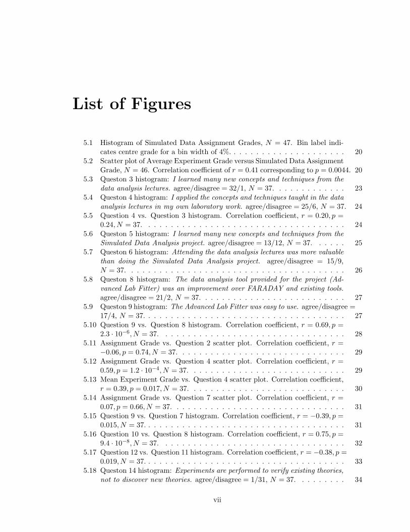
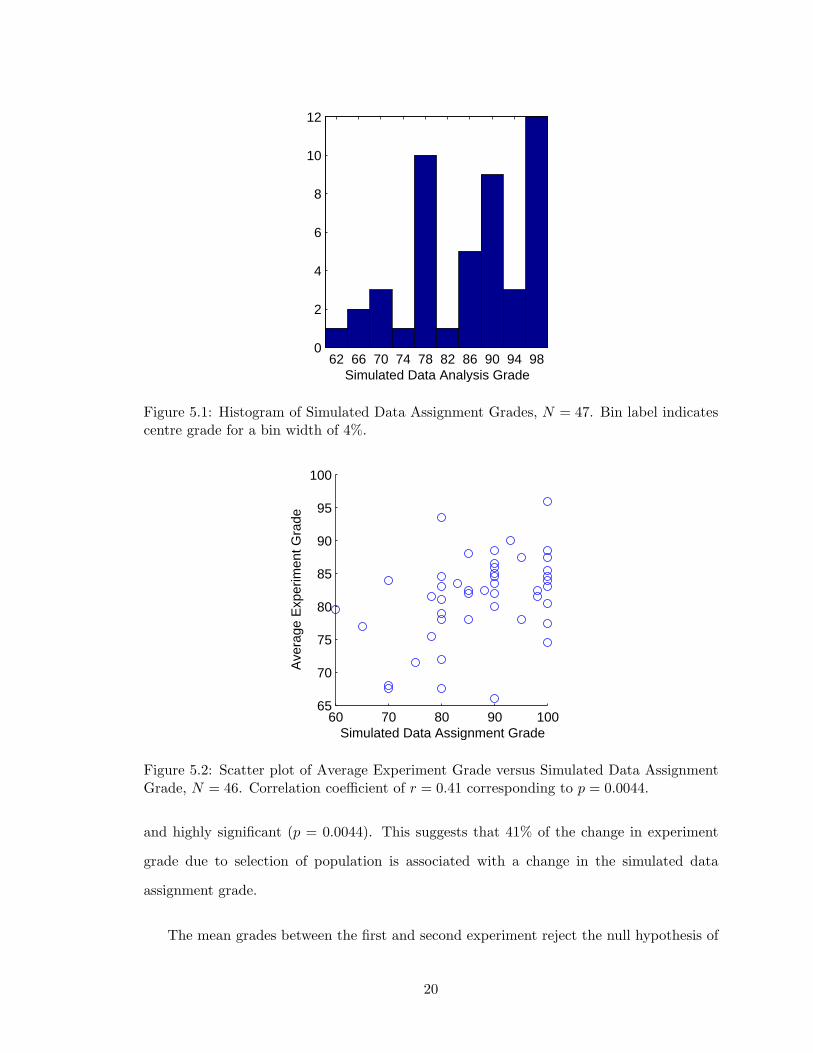
5.1 Histogram of Simulated Data Assignment Grades, N = 47. Bin label indi-cates centre grade for a bin width of 4%. . . . . . . . . . . . . . . . . . . . . 20

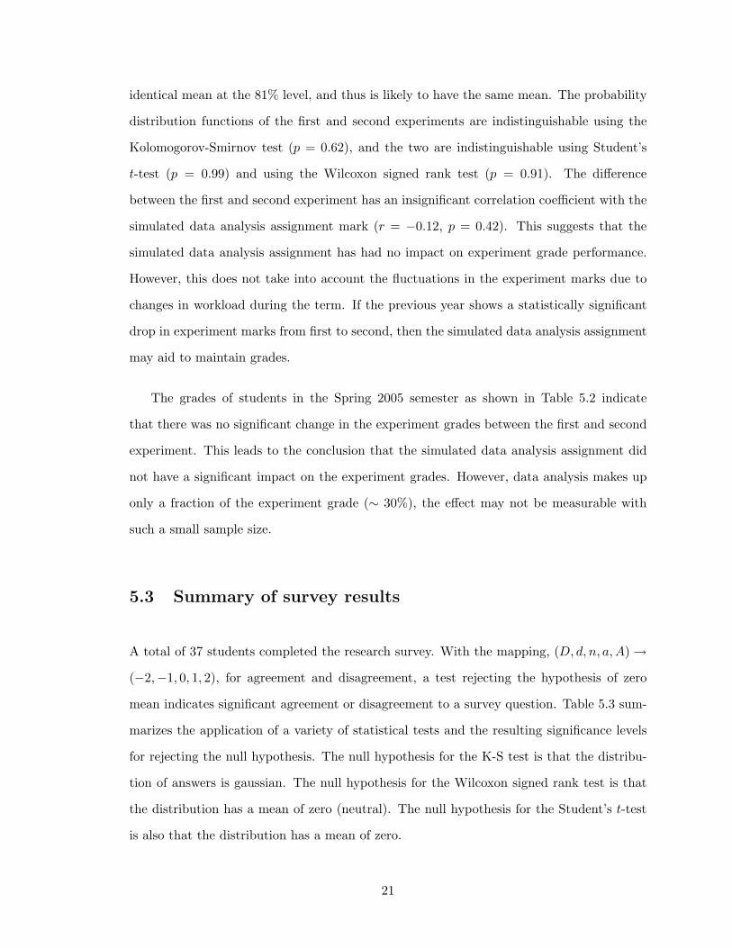
5.2 Scatter plot of Average Experiment Grade versus Simulated Data AssignmentGrade, N = 46. Correlation coefficient of r = 0.41 corresponding to p = 0.0044. 20

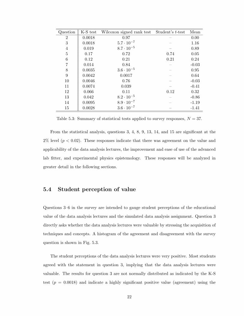
5.3 Queston 3 histogram: I learned many new concepts and techniques from thedata analysis lectures. agree/disagree = 32/1, N = 37. . . . . . . . . . . . . 23

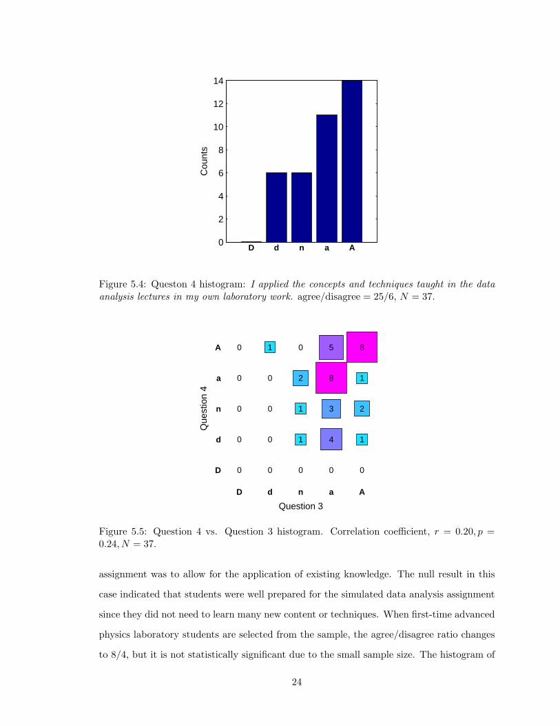
5.4 Queston 4 histogram: I applied the concepts and techniques taught in the dataanalysis lectures in my own laboratory work. agree/disagree = 25/6, N = 37. 24

5.5 Question 4 vs. Question 3 histogram. Correlation coefficient, r = 0.20, p =0.24, N = 37. . . . . . . . . . . . . . . . . . . . . . . . . . . . . . . . . . . . 24

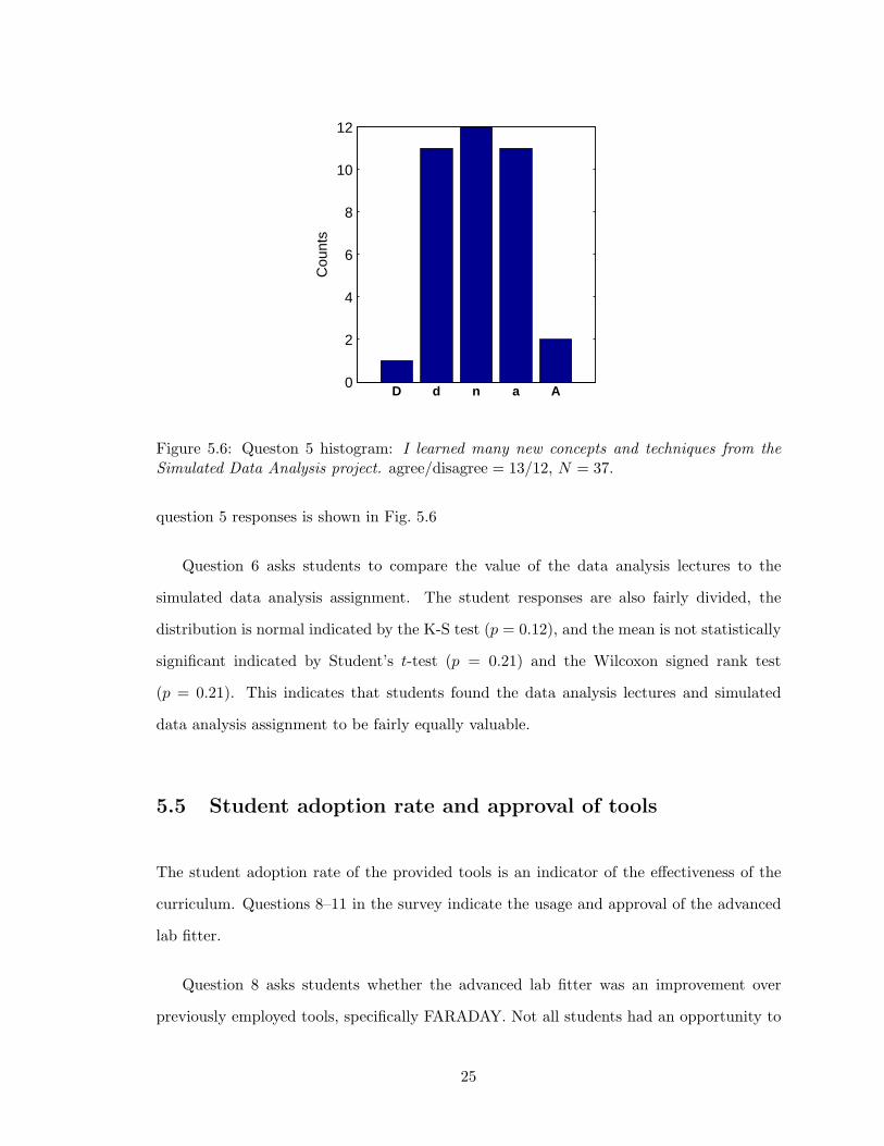
5.6 Queston 5 histogram: I learned many new concepts and techniques from theSimulated Data Analysis project. agree/disagree = 13/12, N = 37. . . . . . 25

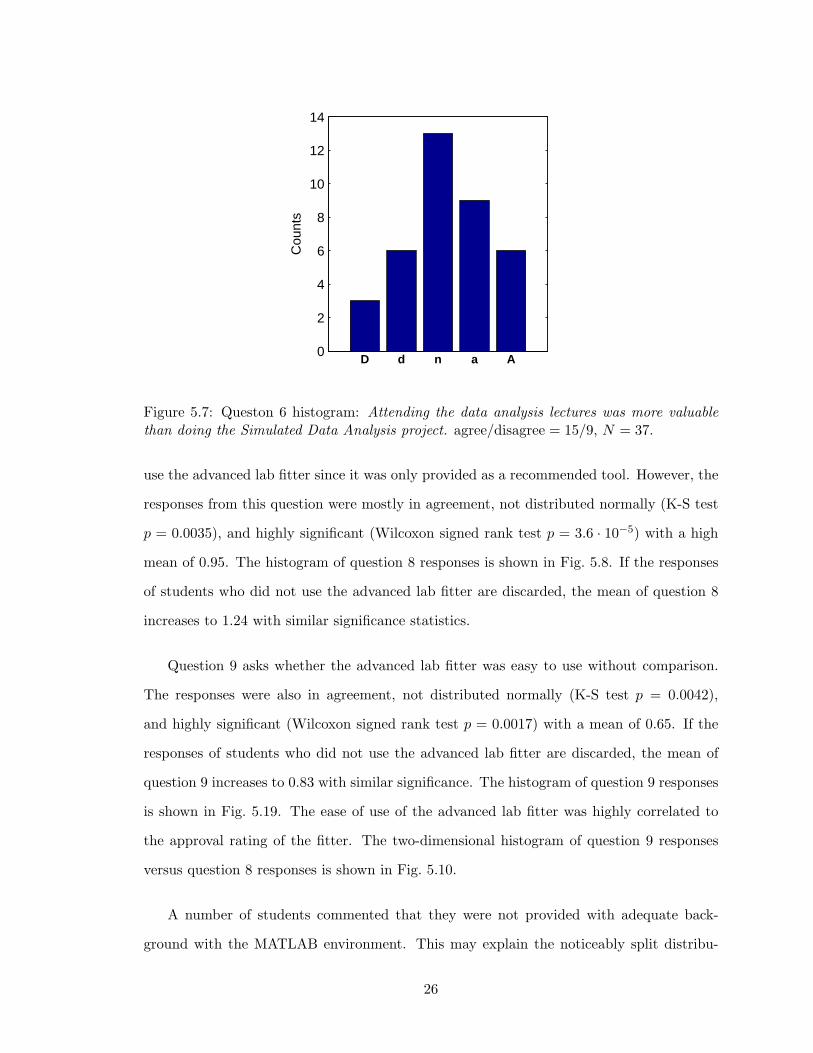
5.7 Queston 6 histogram: Attending the data analysis lectures was more valuablethan doing the Simulated Data Analysis project. agree/disagree = 15/9,N = 37. . . . . . . . . . . . . . . . . . . . . . . . . . . . . . . . . . . . . . . 26

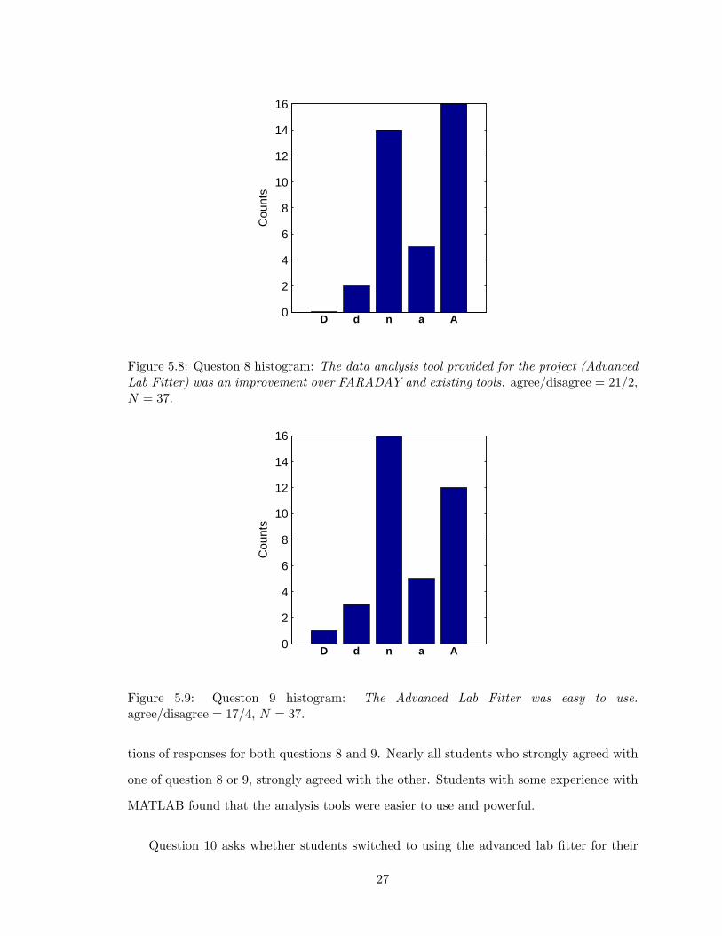
5.8 Queston 8 histogram: The data analysis tool provided for the project (Ad-vanced Lab Fitter) was an improvement over FARADAY and existing tools.agree/disagree = 21/2, N = 37. . . . . . . . . . . . . . . . . . . . . . . . . . 27

5.9 Queston 9 histogram: The Advanced Lab Fitter was easy to use. agree/disagree =17/4, N = 37. . . . . . . . . . . . . . . . . . . . . . . . . . . . . . . . . . . . 27

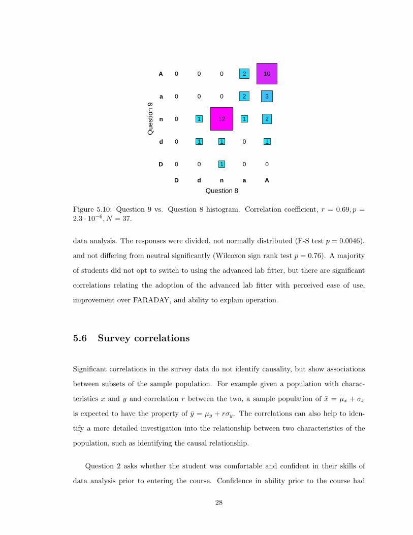
5.10 Question 9 vs. Question 8 histogram. Correlation coefficient, r = 0.69, p =2.3 · 10−6, N = 37. . . . . . . . . . . . . . . . . . . . . . . . . . . . . . . . . 28

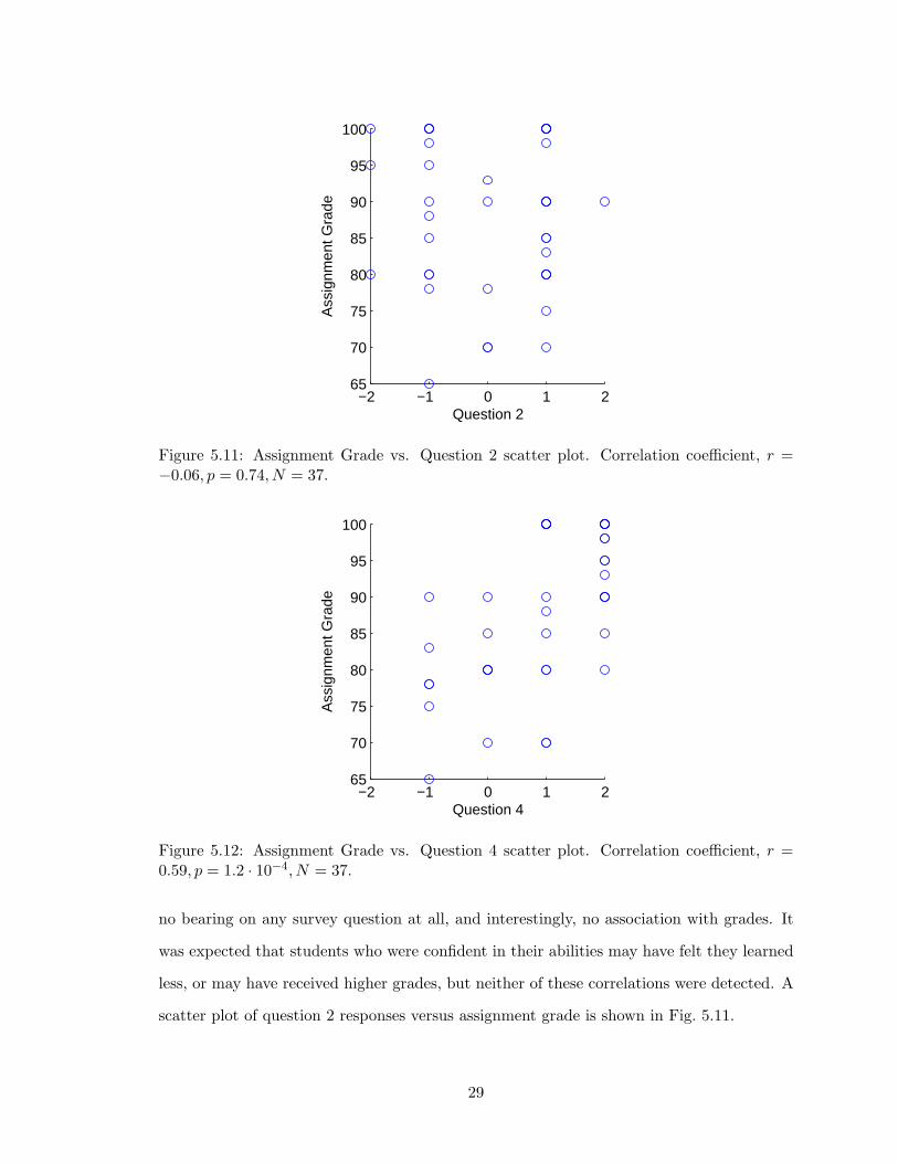
5.11 Assignment Grade vs. Question 2 scatter plot. Correlation coefficient, r =−0.06, p = 0.74, N = 37. . . . . . . . . . . . . . . . . . . . . . . . . . . . . . 29

5.12 Assignment Grade vs. Question 4 scatter plot. Correlation coefficient, r =0.59, p = 1.2 · 10−4, N = 37. . . . . . . . . . . . . . . . . . . . . . . . . . . . 29

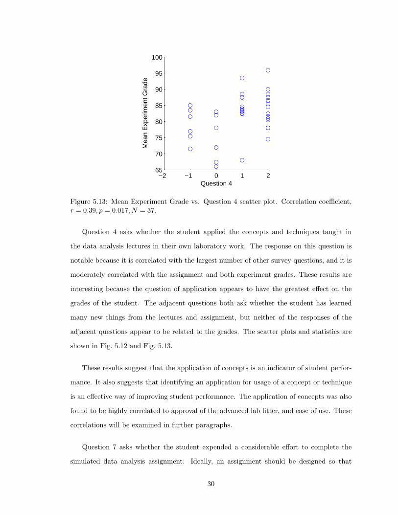
5.13 Mean Experiment Grade vs. Question 4 scatter plot. Correlation coefficient,r = 0.39, p = 0.017, N = 37. . . . . . . . . . . . . . . . . . . . . . . . . . . . 30

5.14 Assignment Grade vs. Question 7 scatter plot. Correlation coefficient, r =0.07, p = 0.66, N = 37. . . . . . . . . . . . . . . . . . . . . . . . . . . . . . . 31

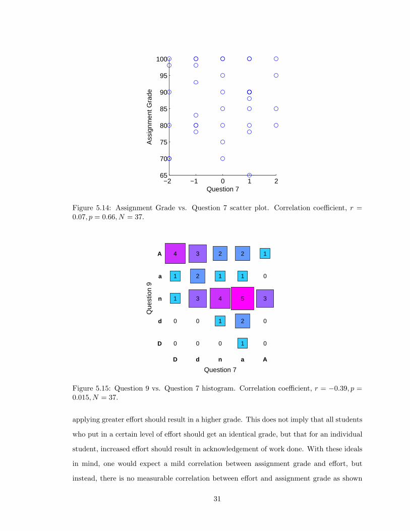
5.15 Question 9 vs. Question 7 histogram. Correlation coefficient, r = −0.39, p =0.015, N = 37. . . . . . . . . . . . . . . . . . . . . . . . . . . . . . . . . . . . 31

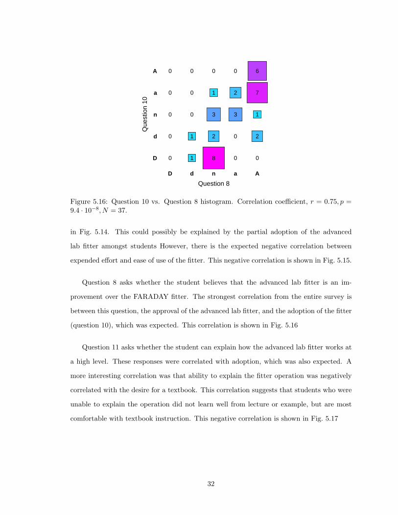
5.16 Question 10 vs. Question 8 histogram. Correlation coefficient, r = 0.75, p =9.4 · 10−8, N = 37. . . . . . . . . . . . . . . . . . . . . . . . . . . . . . . . . 32

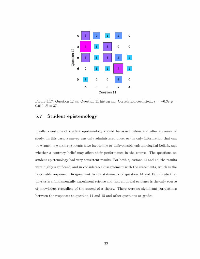
5.17 Question 12 vs. Question 11 histogram. Correlation coefficient, r = −0.38, p =0.019, N = 37. . . . . . . . . . . . . . . . . . . . . . . . . . . . . . . . . . . . 33

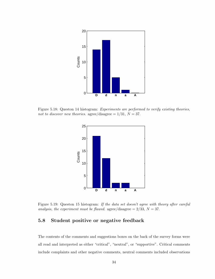
5.18 Queston 14 histogram: Experiments are performed to verify existing theories,not to discover new theories. agree/disagree = 1/31, N = 37. . . . . . . . . 34

vii

5.19 Queston 15 histogram: If the data set doesn’t agree with theory after carefulanalysis, the experiment must be flawed. agree/disagree = 2/33, N = 37. . . 34

A.1 The Data Preview and Browser. . . . . . . . . . . . . . . . . . . . . . . . . 42A.2 Sample labelled data preview. . . . . . . . . . . . . . . . . . . . . . . . . . . 43A.3 The Fitting Tool. . . . . . . . . . . . . . . . . . . . . . . . . . . . . . . . . . 44A.4 Successful fit using the Fitting Tool. . . . . . . . . . . . . . . . . . . . . . . 45

viii

List of Tables

2.1 Dimensions of student expectations from the MPEX survey. . . . . . . . . . 3

3.1 Grading scheme for the advanced physics laboratory for Fall 2005. . . . . . 63.2 Grading scheme for the advanced physics laboratory for Spring 2006 (updated). 8

5.1 Summary of grades for Spring 2006 semester, N = 47. . . . . . . . . . . . . 195.2 Summary of grades for Spring 2005 semester, N = 73. . . . . . . . . . . . . 195.3 Summary of statistical tests applied to survey responses, N = 37. . . . . . . 225.4 Summary of student comments and suggestions from survey forms, N = 37. 35

C.1 Response to question 0, N = 37. . . . . . . . . . . . . . . . . . . . . . . . . 59C.2 Response to question 1, N = 37. . . . . . . . . . . . . . . . . . . . . . . . . 59C.3 Summary of responses, N = 37. . . . . . . . . . . . . . . . . . . . . . . . . . 59

ix

Chapter 1

Introduction

Quantitative data analysis is a common feature of all scientific disciplines. As a construc-

tivist discipline, science depends on the appropriate analysis of reliable experimental data to

reach sound conclusions. Students in the sciences are often called to perform such analyses

in laboratories throughout their respective coursework and are evaluated upon their use of

tools and judgment. However, there are notable gaps between the formal instruction given

to students and the expectations of students with respect to data analysis.

Without formal instruction of data analysis, instructors may unknowingly set an invis-

ible bar for students to reach for. Instructors have a particular expectation in mind for

students, but the students may be unaware of it. In the following chapters, techniques from

physics education research will be applied to the discipline of quantitative data analysis in

order to develop a curriculum module for upper year undergraduate students. The back-

ground theory and motivation will be outlined allowing for a discussion of the design and

implementation of the curriculum with respect to aspects of the theory. Then, an evaluation

methodology will be presented, followed by the presentation of the results of the evaluation

and a critical analysis of the design, results, and implications. Finally, the further work on

the subject will be described as well as the conclusions of this research study.

1

Chapter 2

Background theory and motivation

Physics education research is a unique multidisciplinary field. It attempts to combine tradi-

tional educational theory and scientific constructivism in a single topic of research. Physics

is a unique field in that its academic community shares many common interpretations about

the nature of the physical world and its theories have widespread acceptance. In this capac-

ity, physicists share a community consensus on the ways of thinking about many features

of the physical world [6]. Redish uses classical mechanics and classical thermodynamics as

examples of areas of study where the agreement is very strong.

A key consequence of this strong consensus is that physicists believe that there are

optimal ways of understanding concepts in physics. This agreement in epistemology has

been studied and highlighted in the development of the Maryland Physics Expectations

survey (MPEX) in which an expert group of American physicists was shown to have 87%

agreement on the nature of understanding physics along six different dimensions [7]. The

MPEX study has influenced many physics education researchers by encouraging the goal

of epistemological sophistication as a key student achievement. Moreover, epistemological

development has been suggested as an effective means of improving student performance,

and has taken a place in the design and evaluation of physics curricula. The dimensions

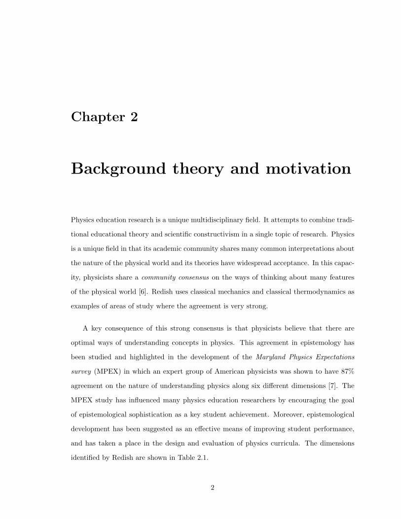
identified by Redish are shown in Table 2.1.

2

Favourable UnfavourableIndependence takes responsibility for construct-

ing own understandingtakes what is given by authorities(teacher, text) without evaluation

Coherence believes physics needs to be con-sidered as a connected, consistentframework

believes physics can be treated asunrelated facts or “pieces”

Concepts stresses understanding of the un-derlying ideas and concepts

focuses on memorizing and usingformulas

Reality link believes ideas learned in physicsare relevant and useful in a widevariety of real contexts

believes ideas learned in physicshave little relation to experiencesoutside the classroom

Math link considers mathematics as a conve-nient way of representing physicalphenomena

views the physics and the mathas independent with little relation-ship between them

Effort makes the effort to use informa-tion available and tries to makesense of it

does not attempt to use availableinformation effectively

Table 2.1: Dimensions of student expectations from the MPEX survey.

The consensus on epistemology has helped to shape the goals of physics education

research, but there are limitations to the usage of student epistemology as a theoretical

framework for physics education. The MPEX study and other studies using the MPEX

study as a metric for effectiveness limit their usage to introductory theoretical physics

courses [5, 2, 7]. The authors’ common focus is on helping students to understand theoretical

concepts and make the assumption that an excellent understanding of concepts implies good

problem solving skills. Perhaps as professional physicists, the authors make the assumption

that the practical set of problem solving skills necessary for even entry-level physics courses

is not trivial. Ehrlich suggests that student epistemology may not be the only explanation

for student performance and that other factors such as intrinsic ability should be considered

[4]. However, Ehrlich may too hastily conclude that some students simply do not have the

ability to do physics. He quotes a student, “. . . hey that course I took with you was great

and really made me think, although I only got a C.” And while it may be convenient to

label such a student as interested in physics without the required ability, it is possible that

the student did not have the tools necessary to solve the examination problems.

Dewey’s theory of education can be roughly interpreted as identifying educational ex-

3

periences as those which add value and meaning to a variety of different ideas and contexts

[3]. Although Dewey’s theory is rooted in traditional philosophy, his pragmatic approach

to education has value when considering physics education research. Some may worry that

a pragmatic view of physics education leads down the slippery slope of a physics education

as career training. However, some practical skills are absolutely necessary in order to be a

successful physics student. Simple algebraic manipulation and basic calculus are two skill

sets that immediately come to mind. So, the teaching of mathematics may be viewed as a

form of necessary physics career training. In an experimental physics context, there many

more practical skills that must be used to interpret scientific experiments. These can range

from the usage of voltmeters and oscilloscopes to the application of statistics to interpret

experimental data.

To summarize, the basic educational theory that will be applied throughout this doc-

ument will be based upon epistemological sophistication and acquisition of practical tools

and techniques.

4

Chapter 3

Design and implementation

In this chapter, the design and implementation of a data analysis curriculum will be pre-

sented. An overview of a current curriculum will be discussed followed by a description of

the proposed tools and assignments and finally a summary of goals in the context of the

theory presented in the previous chapter.

3.1 The advanced physics laboratory

The advanced physics laboratory is an undergraduate experimental physics course offered at

the University of Toronto. It is taken by upper year (third and fourth year) undergraduate

students in the Physics and Engineering Science programs at the university. The typical

enrollment into the course is around fifty to seventy students per semester.

3.1.1 Previous curriculum

The course curriculum is based upon a series of three (3) in-depth laboratory experiments

of which students have a degree of choice in selecting. These experiments are usually classic

experiments in modern and quantum physics. Examples include calculating particle decay

5

lifetimes, investigating crystal diffraction patterns, and characterizing the statistical me-

chanics of macroscopic granular material. In addition, each student is assigned a supervis-

ing professor and the aid of a lab demonstrator. Throughout the experiments, the students

are required to complete a series of mandatory exercises, but are given the flexibility to pur-

sue other interesting aspects of the experiments and to use a variety of analysis methods.

Each student is required to keep a detailed laboratory notebook with their analysis and

notes. Each experiment mark is based on a combination of their laboratory technique from

informal conversations in the lab, the quality of their analysis presented in their laboratory

notebook, and their understanding of the material as indicated by a formal interview with

the supervising professor.

In addition to the experiments, the students are required to prepare a formal report

of their results of a single experiment, and at the very end of the course, there is an oral

examination which is intended to cover all aspects of the experiments performed through

the semester. The oral examination is conducted by two of the supervising professors, and

one lab demonstrator. The grading scheme for the course is shown in Table 3.1.

Experiment grades 63%Formal report 17%Oral examination 20%

Table 3.1: Grading scheme for the advanced physics laboratory for Fall 2005.

Most students in the advanced physics laboratory have had at least two semesters of

experimental physics in previous years. The course is a program requirement for Engineering

Science students, while it is a technical elective for Physics students.

3.1.2 Existing data analysis curriculum

The previous course curriculum provided no formal data analysis instruction. The students

were expected to carry their analysis skills from the first and second year laboratory courses

and apply them in the advanced laboratory. However, there is a gap in the material taught

between the introductory labs and the advanced labs. The first year labs emphasize con-

6

ceptual understanding and downplay the statistical and mathematical rigour necessary for

a defensible scientific investigation. The second year labs put an emphasis on using vari-

ous kinds of data acquisition equipment such as oscilloscopes, voltmeters, ammeters, and

recording devices. However, the role and estimation of errors in the data analysis is mostly

overlooked. Through the first two years, the only formal evaluation of the understanding of

error analysis in a laboratory setting is the ERRTEST program. The ERRTEST program is

an interactive error analysis quiz that is administered on the computer terminals available

in the undergraduate labs. It is short (roughly 15–30 minutes), given relatively small weight

(5% course grade), and is unsupervised. It is not uncommon for students to collaborate on

multiple tests in order to obtain higher marks.

The physics department also provides the FARADAY fitter as a data analysis tool for

undergraduate students. It is a black-box fitter that employs a web interface to fit user-

inputted data to polynomial equations. It is also able to calculate χ2 probabilities and

estimate the errors on parameters.

3.2 Proposed course additions

For this research study, some additions to the advanced physics laboratory have been pro-

posed and implemented. They are the deployment of the advanced lab fitter, intended

to supercede the FARADAY tool, and the creation of formally taught course material re-

garding data and error analysis. The additions to the course material include a set of

error analysis lectures delivered by one of the supervising professors, and a data analysis

assignment. These additions are outlined in more details in the following sections and all

associated documentation and source files are included in the appendices. The addition

of the data analysis assignment changes the grading scheme for the updated course. The

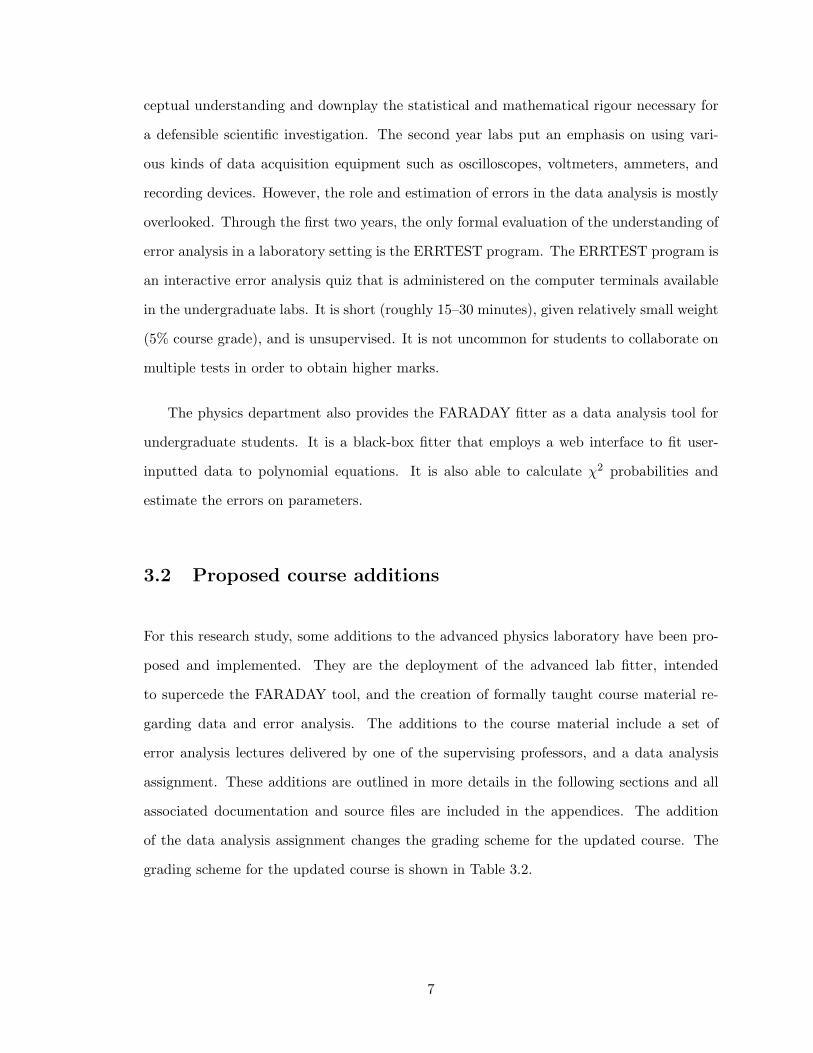
grading scheme for the updated course is shown in Table 3.2.

7

Experiment grades 60%Simulated data analysis assignment 5%Formal report 15%Oral examination 20%

Table 3.2: Grading scheme for the advanced physics laboratory for Spring 2006 (updated).

3.2.1 The advanced lab fitter

The initial reason for designing the advanced lab fitter was to provide a more powerful

fitting tool for students in the advanced physics laboratory. However, there are a number

of pedagogical implications of providing a new tool. The advanced lab fitter can be consid-

ered with respect to the epistemological framework provided in the previous chapter and

additionally (and moreso) as the acquisition of a practical tool and technique.

The advanced lab fitter is built upon a series of MATLAB functions and scripts, and

represents a precise implementation of the fitting technique outlined in the data analysis

lectures [1]. Since the entire source is provided with the fitter, interested students can

examine the operations that the fitter performs to produce its plots unlike previous tools.

This open piece of software appeals to the Independence and Concepts dimensions in the

epistemological framework. Even though the operation of the fitter is outlined in the lec-

tures, students are provided with the opportunity to learn from a fairly accessible example

of a fitter.

The fitter is also sufficiently sophisticated that it is used in some physics research labs

at the university. This high level of functionality appeals to the Reality link dimension.

The usage in the field identifies the tool as relevant outside of the classroom and gives it a

degree of validity. Students benefit from performing analysis which are not artificial, but

as justifiable as those performed in academic research.

Finally, the ease of use of the tool appeals to the Effort dimension. This may seem

counterintuitive at first. How can providing an easy route encourage increased efforts? The

answer can be shown by considering where students place their efforts when performing

8

an analysis with the fitter. Efforts can be divided between the usage of the tools and the

interpretation of the data. If more time and effort is spent simply using the tools, then

students will not be able to make effective use of the data. It is easier to “play” with data

when the analysis tools are more transparent.

The fitter also clearly fulfills a practical purpose. The fitter provides all the necessarily

functionality for parametric analysis and acts as a springboard to apply the techniques

taught in the data analysis lectures. It is also a piece of software that can be easily used

for any of the analysis tasks in the laboratory exercises and research projects.

3.2.2 Data analysis lectures

The data analysis lectures were delivered during the first weeks of the semester, while the

students were engaged in their first experiments. The lectures were also supplemented

with a set of notes that explain mathematical derivations in some detail. The purpose of

the data analysis lectures were to complement the simulated data analysis assignment and

vice versa. A lecture has limited effectiveness, as evaluated through the epistemological

dimensions identified in the previous chapter. However where the lecture-based teaching

lacks, the analysis assignment excels.

Lecture-based teaching has been shown to at best neutrally affect the independence di-

mension. The nature of lecture-based teaching lends itself to the mentality of an authority

figure dispensing the undisputed truth. It also typically negatively affects the effort dimen-

sion as students are passive participants in the exchange, and often have answers spoonfed

to them. Although they have limitations, lectures are excellent at improving student epis-

temologies along the coherence, concepts, and math link dimensions.

The step-by-step derivations and usage of mathematical tools to explain data analysis

allow students to see the statistical underpinnings of their analysis. This approach not

only helps the Math link dimension, but allows students to grasp the underlying concepts

that the statistical analysis are based upon. The explanations also help along the reality

9

link dimension by educating students how most data fitters used by researchers operate. A

skilled instructor will also be able to show how data analysis fits into a systematic approach

to experimental physics, thus improving the coherence dimension.

The data analysis lectures also serve to appeal to the different learning styles of the

students in the laboratory. While some students may benefit from the practice of crunching

numbers in the simulated data analysis assignment, many find that mathematical deriva-

tions are the most effective way of assimilating a body of knowledge.

3.2.3 The simulated data analysis assignment

The simulated data analysis assignment was conceived to isolate the data analysis portion

of the laboratory exercise. In a typical laboratory exercise, a student must worry not

only about the validity of the results, but also the quality of the data. If the data is of

questionable quality, then an analysis will yield limited information. By generating data

of uniform quality, and separating the analysis from the laboratory experiments, students

have the ability to focus on performing a well justified analysis.

The assignment provides each student with a unique set of data corresponding to two

statistical data analysis problems. The first problem is a spectral analysis, where students

are asked to characterize a gaussian peak on a quadratic background with a few parameters.

The second problem is an exponential fit to some voltage data. Each data set is generated

along with a solution provided by the advanced lab fitter. The course coordinator retains

the solution manual, while the students are given numbered assignments each with unique

data. The analysis was weighted as shown in Table. 3.2 and was marked by the course

coordinator.

The simulated data analysis assignment has value and strength where the lectures are

weak, such as the independence and effort dimensions of the epistemology theory. While a

systematic approach can be taken to the assignment, there is no single correct approach to

answering the questions. This allows students to seek solutions independently, and construct

10

understanding from their own perspectives. The assignment is also open ended. There are

many statistical features of the data that can be analyzed and various tests of significance

can be applied to ensure the analysis is valid. The open ended nature of the assignment

appeals to the effort dimension, by providing students the opportunity to make the most of

a limited amount of data. And since the data is known to fit a model, analyses of greater

depth will only assure confidence in the results.

There is also a strong benefit to the Reality link aspect of the theory. Students are

expected to produce an analysis at a quality level that is expected of their notebook. So,

this serves as a test bed for students to make “free” mistakes without impacting the quality

of their work, since small mistakes can lead to great misunderstandings when applied to an

entire experimental system. Outside of the six dimensions identified by the MPEX survey,

an opportunity to use advanced tools for a data analysis problem is highly practical. The

assignment can provide training for data analysis outside of the laboratory, since the tools

are used for analysis in academic research.

3.3 Course schedule

Ideally, the data analysis lectures and the simulated data analysis assignment would be

given out prior to any of the experiments so that the skills and knowledge gained could

be applied to the semester’s work. However, due to the scheduling of the supervising

professors, the experiment schedule could not be modified. So, the lectures were provided

and the simulated data analysis assignment was distributed during the first experiment

period. The data analysis assignment was due shortly after the first experiment deadline.

This schedule also allows for a limited pre/post effect analysis between the first and

second experiment. While students may not have had the opportunity to assimilate and

apply the skills from the lectures and assignment in their first experiment, they would be

able to in their second. The usage of grades and other metrics of student performance are

outlined in the next chapter.

11

Chapter 4

Evaluation methodology

In this chapter, the approaches to evaluate the effectiveness of the curriculum additions are

outlined. There are a few basic indicators of effectiveness that have been selected. These

indicators are, the student adoption and approval of tools, student perceptions of the value

of learning, student performance on the assignment, positive and negative feedback on the

assignment and fitter, and correlations of performance to epistemological beliefs.

4.1 Student feedback and survey

In order to identify indicators of effectiveness, a student survey and feedback form was

created and distributed to the students after they had attended the data analysis lectures,

completed the simulated data analysis assignment, received their grades and got feedback

from the course coordinator who graded them. The survey was anonymous, but attached

to the assignment identification number so that paired analysis could be conducted. The

full text of the survey is available in the appendix.

The survey was sixteen questions long, fourteen of which were questions based on a

Likert scaling. That is, students were presented with statements and asked to respond in

agreement or disagreement. Each question had five choices, “strongly disagree” (D), “some-

12

what disagree” (d), “neutral” (n), “somewhat agree” (a), and “strongly agree” (A). This

kind of scaling method allowed for simple statistical analysis of the data instead of having to

establish predefined relationships between question choices for an arbitrary multiple choice

survey.

The questions of the survey focused primarily on the previously listed indicators of

effectiveness. In addition, there were several questions that were asked in order to verify

some assumptions about the expectations of students. For example, the survey asks students

their perception of effort expended on the assignment, which was compared to the grades

on the assignment.

4.2 Statistical methods

Agreement and disagreement values were assigned to each question response so that a

neutral response corresponds to zero and strong responses have twice the weight of weaker

ones. Thus, (D, d, n, a,A) → (−2,−1, 0, 1, 2) was selected as the mapping for the responses.

This mapping allows for simple statistical analysis to be applied.

In this analysis, the key method of evaluating the teaching methodology was statisti-

cal methods. The primary statistical tests chosen were the Student’s t-test, and p-tests

for various statistics including the Pearson coefficient, the Kolomogorov-Smirnov test, and

Wilcoxon signed rank test. A statistically significant result is identified at the 2% level.

This means that when comparing two statistical distributions, the test would produce a

result at least as extreme as the measured result less than once in fifty experimental runs

if they were identical distributions.

4.2.1 Kolmogorov-Smirnov test

The Kolmogorov-Smirnov (K-S) test is used to determine if a set of data obeys a particular

statistical distribution. For survey data, one cannot make the assumption that the answers

13

to the survey follow a normal distribution or Student’s t-distribution. The K-S test ensures

that an appropriate hypothesis testing method is used for the survey data. To apply the

K-S test, the empirical cumulative distribution function is calculated and compared to

a theoretical cumulative distribution function. The absolute maximum between the two

functions defines a statistic with a particular probability distribution function that will

indicate whether the sample data corresponds to the theoretical statistical distribution.

The Kolmogorov-Smirnov test is implemented in MATLAB using the kstest function.

4.2.2 Wilcoxon signed rank test

The Wilcoxon signed rank test can be used to identify whether paired observations with

an arbitrary probability distribution differ significantly. To apply the Wilcoxon signed

rank test, the differences of the paired observations are calculated and ranked. The ranks

associated with positive differences are summed to define a statistic. This statistic has a

particular probability distribution function that can identify whether there is a significant

difference between the paired observations with a given probability.

The Wilcoxon signed rank test is implemented in MATLAB using the signrank func-

tion.

4.2.3 Student’s t-tests

Student’s t-distribution is a statistical distribution published by William Gossett in 1908. It

describes the probability distribution for random variable t without knowing the population

standard deviation of a sample. In the limit of a large sample size, the t-distribution

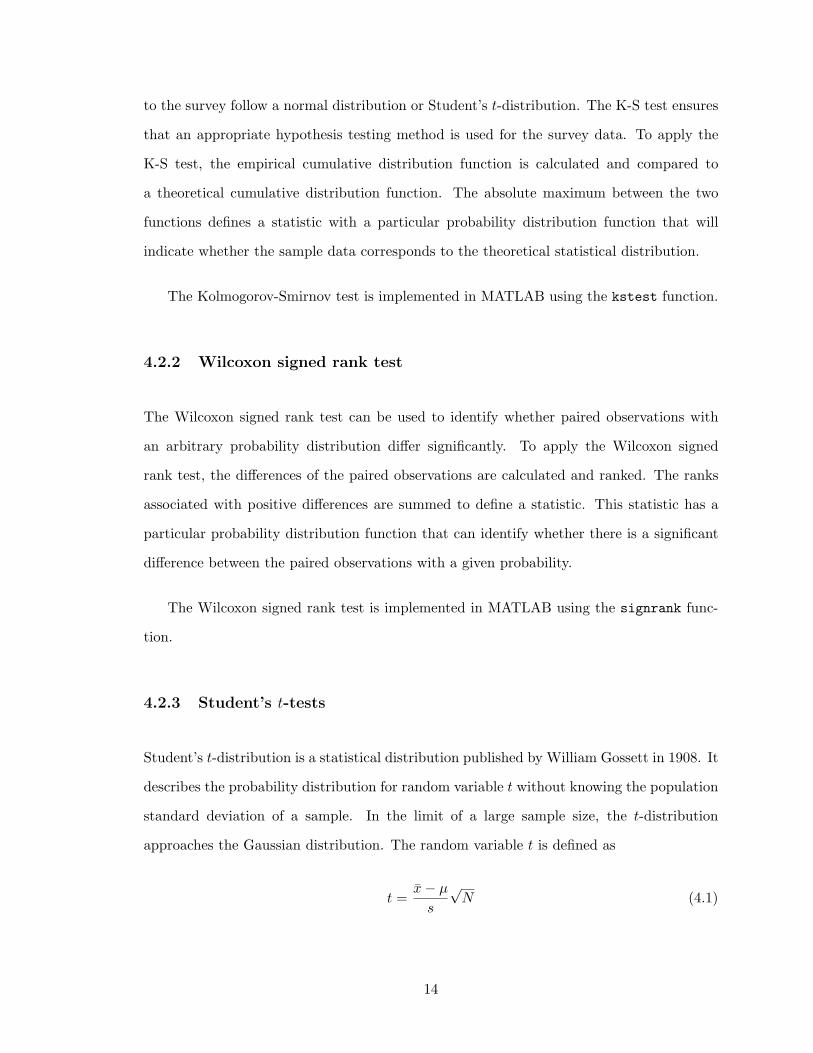
approaches the Gaussian distribution. The random variable t is defined as

t =x− µ

s

√N (4.1)

14

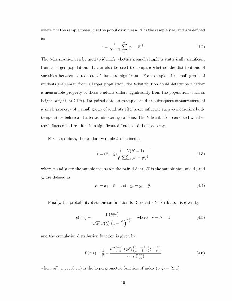
where x is the sample mean, µ is the population mean, N is the sample size, and s is defined

as

s =1

N − 1

N∑

i=1

(xi − x)2. (4.2)

The t-distribution can be used to identify whether a small sample is statistically significant

from a larger population. It can also be used to compare whether the distributions of

variables between paired sets of data are significant. For example, if a small group of

students are chosen from a larger population, the t-distribution could determine whether

a measurable property of those students differs significantly from the population (such as

height, weight, or GPA). For paired data an example could be subsequent measurements of

a single property of a small group of students after some influence such as measuring body

temperature before and after administering caffeine. The t-distribution could tell whether

the influence had resulted in a significant difference of that property.

For paired data, the random variable t is defined as

t = (x− y)

√N(N − 1)∑Ni=1(xi − yi)2

(4.3)

where x and y are the sample means for the paired data, N is the sample size, and xi and

yi are defined as

xi = xi − x and yi = yi − y. (4.4)

Finally, the probability distribution function for Student’s t-distribution is given by

p(r; t) =Γ(

r+12

)

√πr Γ

(r2

) (1 + t2

r

) r+12

where r = N − 1 (4.5)

and the cumulative distribution function is given by

P (r; t) =12

+t Γ

(r+12

)2F1

(12 , r+1

2 ; 32 ;− t2

r

)

√πr Γ

(r2

) (4.6)

where 2F1(a1, a2; b1; x) is the hypergeometric function of index (p, q) = (2, 1).

15

The Student’s t-test is implemented in MATLAB using the ttest and ttest2 functions.

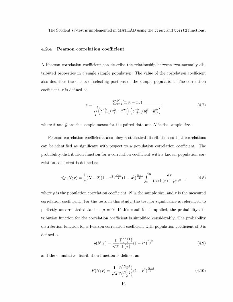
4.2.4 Pearson correlation coefficient

A Pearson correlation coefficient can describe the relationship between two normally dis-

tributed properties in a single sample population. The value of the correlation coefficient

also describes the effects of selecting portions of the sample population. The correlation

coefficient, r is defined as

r =∑N

i=1(xiyi − xy)√(∑Ni=1(x

2i − x2)

)(∑Ni=1(y

2i − y2)

) (4.7)

where x and y are the sample means for the paired data and N is the sample size.

Pearson correlation coefficients also obey a statistical distribution so that correlations

can be identified as significant with respect to a population correlation coefficient. The

probability distribution function for a correlation coefficient with a known population cor-

relation coefficient is defined as

p(ρ,N ; r) =1π

(N − 2)(1− r2)N−4

2 (1− ρ2)N−1

2

∫ ∞

0

dx

(cosh(x)− ρr)N−1(4.8)

where ρ is the population correlation coefficient, N is the sample size, and r is the measured

correlation coefficient. For the tests in this study, the test for significance is referenced to

perfectly uncorrelated data, i.e. ρ = 0. If this condition is applied, the probability dis-

tribution function for the correlation coefficient is simplified considerably. The probability

distribution function for a Pearson correlation coefficient with population coefficient of 0 is

defined as

p(N ; r) =1√π

Γ(

r+12

)

Γ(

r2

) (1− r2)r−22 (4.9)

and the cumulative distribution function is defined as

P (N ; r) =1√π

Γ(

N−12

)

Γ(

N−22

)(1− r2)N−4

2 . (4.10)

16

The Pearson correlation coefficient is implemented in MATLAB using the corrcoef

function.

17

Chapter 5

Analysis and results

5.1 Summary of student grades

A summary of the grades for the Spring 2006 semester are shown in Table 5.1. A summary

of the grades for the Spring 2005 semester are shown in Table 5.2. The experiments were

marked by a variety of supervising professors in both years, while the simulated data analysis

assignment was marked only by the course coordinator.

The entire sample of students were divided into four different sample groups for ini-

tial analysis. The sample groups were the physics students, the engineering students, the

students who chose experiment A in the simulated data analysis assignment, and those

who chose experiment B. There were no significant variations between the different samples

or between the experiment marks. The grades on the simulated data analysis assignment

were slightly higher than those on the experiments, but otherwise there were no significant

features of the data.

The experiment grades for the previous year are shown for comparison. The grades

for the engineers in spring of 2005 were greater than those of the physics students and

statistically significant. The K-S test and Student’s t-test reject the hypothesis of identical

18

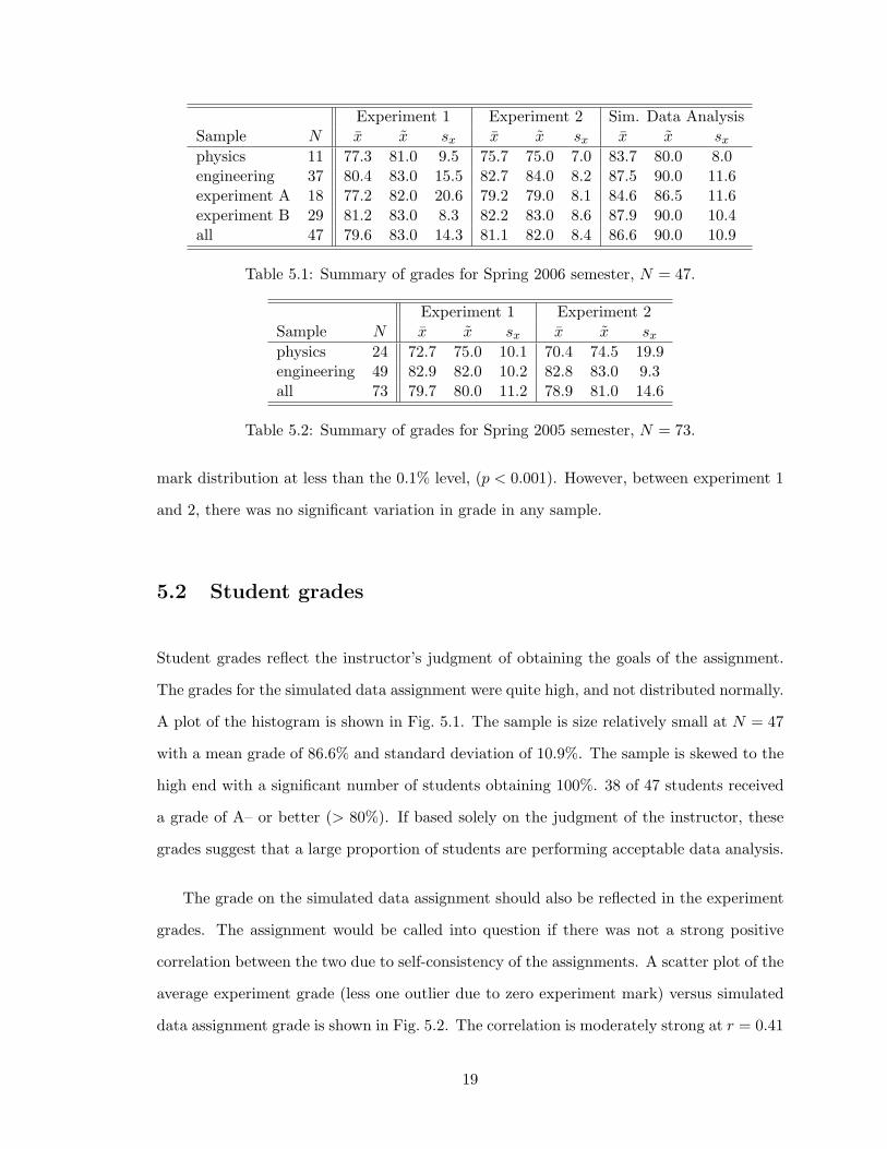
Experiment 1 Experiment 2 Sim. Data AnalysisSample N x x sx x x sx x x sx

physics 11 77.3 81.0 9.5 75.7 75.0 7.0 83.7 80.0 8.0engineering 37 80.4 83.0 15.5 82.7 84.0 8.2 87.5 90.0 11.6experiment A 18 77.2 82.0 20.6 79.2 79.0 8.1 84.6 86.5 11.6experiment B 29 81.2 83.0 8.3 82.2 83.0 8.6 87.9 90.0 10.4all 47 79.6 83.0 14.3 81.1 82.0 8.4 86.6 90.0 10.9

Table 5.1: Summary of grades for Spring 2006 semester, N = 47.

Experiment 1 Experiment 2Sample N x x sx x x sx

physics 24 72.7 75.0 10.1 70.4 74.5 19.9engineering 49 82.9 82.0 10.2 82.8 83.0 9.3all 73 79.7 80.0 11.2 78.9 81.0 14.6

Table 5.2: Summary of grades for Spring 2005 semester, N = 73.

mark distribution at less than the 0.1% level, (p < 0.001). However, between experiment 1

and 2, there was no significant variation in grade in any sample.

5.2 Student grades

Student grades reflect the instructor’s judgment of obtaining the goals of the assignment.

The grades for the simulated data assignment were quite high, and not distributed normally.

A plot of the histogram is shown in Fig. 5.1. The sample is size relatively small at N = 47

with a mean grade of 86.6% and standard deviation of 10.9%. The sample is skewed to the

high end with a significant number of students obtaining 100%. 38 of 47 students received

a grade of A– or better (> 80%). If based solely on the judgment of the instructor, these

grades suggest that a large proportion of students are performing acceptable data analysis.

The grade on the simulated data assignment should also be reflected in the experiment

grades. The assignment would be called into question if there was not a strong positive

correlation between the two due to self-consistency of the assignments. A scatter plot of the

average experiment grade (less one outlier due to zero experiment mark) versus simulated

data assignment grade is shown in Fig. 5.2. The correlation is moderately strong at r = 0.41

19

62 66 70 74 78 82 86 90 94 980

2

4

6

8

10

12

Simulated Data Analysis Grade

Figure 5.1: Histogram of Simulated Data Assignment Grades, N = 47. Bin label indicatescentre grade for a bin width of 4%.

60 70 80 90 10065

70

75

80

85

90

95

100

Simulated Data Assignment Grade

Ave

rage

Exp

erim

ent G

rade

Figure 5.2: Scatter plot of Average Experiment Grade versus Simulated Data AssignmentGrade, N = 46. Correlation coefficient of r = 0.41 corresponding to p = 0.0044.

and highly significant (p = 0.0044). This suggests that 41% of the change in experiment

grade due to selection of population is associated with a change in the simulated data

assignment grade.

The mean grades between the first and second experiment reject the null hypothesis of

20

identical mean at the 81% level, and thus is likely to have the same mean. The probability

distribution functions of the first and second experiments are indistinguishable using the

Kolomogorov-Smirnov test (p = 0.62), and the two are indistinguishable using Student’s

t-test (p = 0.99) and using the Wilcoxon signed rank test (p = 0.91). The difference

between the first and second experiment has an insignificant correlation coefficient with the

simulated data analysis assignment mark (r = −0.12, p = 0.42). This suggests that the

simulated data analysis assignment has had no impact on experiment grade performance.

However, this does not take into account the fluctuations in the experiment marks due to

changes in workload during the term. If the previous year shows a statistically significant

drop in experiment marks from first to second, then the simulated data analysis assignment

may aid to maintain grades.

The grades of students in the Spring 2005 semester as shown in Table 5.2 indicate

that there was no significant change in the experiment grades between the first and second

experiment. This leads to the conclusion that the simulated data analysis assignment did

not have a significant impact on the experiment grades. However, data analysis makes up

only a fraction of the experiment grade (∼ 30%), the effect may not be measurable with

such a small sample size.

5.3 Summary of survey results

A total of 37 students completed the research survey. With the mapping, (D, d, n, a,A) →(−2,−1, 0, 1, 2), for agreement and disagreement, a test rejecting the hypothesis of zero

mean indicates significant agreement or disagreement to a survey question. Table 5.3 sum-

marizes the application of a variety of statistical tests and the resulting significance levels

for rejecting the null hypothesis. The null hypothesis for the K-S test is that the distribu-

tion of answers is gaussian. The null hypothesis for the Wilcoxon signed rank test is that

the distribution has a mean of zero (neutral). The null hypothesis for the Student’s t-test

is also that the distribution has a mean of zero.

21

Question K-S test Wilcoxon signed rank test Student’s t-test Mean2 0.0018 0.97 – 0.003 0.0018 5.7 · 10−7 – 1.164 0.019 8.7 · 10−5 – 0.895 0.17 0.72 0.74 0.056 0.12 0.21 0.21 0.247 0.014 0.84 – -0.038 0.0035 3.6 · 10−5 – 0.959 0.0042 0.0017 – 0.6410 0.0046 0.76 – -0.0311 0.0074 0.039 – -0.4112 0.066 0.11 0.12 0.3213 0.042 8.2 · 10−5 – -0.8614 0.0095 8.9 · 10−7 – -1.1915 0.0028 3.6 · 10−7 – -1.41

Table 5.3: Summary of statistical tests applied to survey responses, N = 37.

From the statistical analysis, questions 3, 4, 8, 9, 13, 14, and 15 are significant at the

2% level (p < 0.02). These responses indicate that there was agreement on the value and

applicability of the data analysis lectures, the improvement and ease of use of the advanced

lab fitter, and experimental physics epistemology. These responses will be analyzed in

greater detail in the following sections.

5.4 Student perception of value

Questions 3–6 in the survey are intended to gauge student perceptions of the educational

value of the data analysis lectures and the simulated data analysis assignment. Question 3

directly asks whether the data analysis lectures were valuable by stressing the acquisition of

techniques and concepts. A histogram of the agreement and disagreement with the survey

question is shown in Fig. 5.3.

The student perceptions of the data analysis lectures were very positive. Most students

agreed with the statement in question 3, implying that the data analysis lectures were

valuable. The results for question 3 are not normally distributed as indicated by the K-S

test (p = 0.0018) and indicate a highly significant positive value (agreement) using the

22

0

5

10

15

20

D d n a A

Cou

nts

Figure 5.3: Queston 3 histogram: I learned many new concepts and techniques from thedata analysis lectures. agree/disagree = 32/1, N = 37.

Wilcoxon signed rank test (p = 5.7 · 10−7).

Question 4 determines whether students applied what they learned from the data anal-

ysis lectures in their own laboratory work. It is clear from the histogram that most students

agreed with the statement in question 4. The distribution is not normal indicated by the

K-S test (p = 0.020), but highly significant as indicated by the Wilcoxon signed rank test

(p = 8.7 · 10−5). The survey results from question 4 are plotted against question 3 in a

two dimensional histogram. A correlation coefficient of the agreements was calculated, but

not found to be significant (p = 0.24). However, those who disagreed to the usage of the

data analysis material agreed to the value of the data analysis lectures. The histogram of

question 4 responses is shown in Fig. 5.4 and the two dimensional histogram of question 4

versus question 3 is shown in Fig. 5.5.

Question 5 asks whether students learned new techniques and concepts from the simu-

lated data analysis assignment. On this question, student responses are fairly divided. The

distribution of responses are normal indicated by the K-S test (p = 0.17) and the agreement

or disagreement in this question is not statistically significant indicated by Student’s t-test

(p = 0.74). This is an expected result, since the purpose of the simulated data analysis

23

0

2

4

6

8

10

12

14

D d n a A

Cou

nts

Figure 5.4: Queston 4 histogram: I applied the concepts and techniques taught in the dataanalysis lectures in my own laboratory work. agree/disagree = 25/6, N = 37.

0

0

0

0

0

0

0

0

0

1

0

1

1

2

0

0

4

3

8

5

0

1

2

1

8

D d n a A

D

d

n

a

A

Question 3

Que

stio

n 4

Figure 5.5: Question 4 vs. Question 3 histogram. Correlation coefficient, r = 0.20, p =0.24, N = 37.

assignment was to allow for the application of existing knowledge. The null result in this

case indicated that students were well prepared for the simulated data analysis assignment

since they did not need to learn many new content or techniques. When first-time advanced

physics laboratory students are selected from the sample, the agree/disagree ratio changes

to 8/4, but it is not statistically significant due to the small sample size. The histogram of

24

0

2

4

6

8

10

12

D d n a A

Cou

nts

Figure 5.6: Queston 5 histogram: I learned many new concepts and techniques from theSimulated Data Analysis project. agree/disagree = 13/12, N = 37.

question 5 responses is shown in Fig. 5.6

Question 6 asks students to compare the value of the data analysis lectures to the

simulated data analysis assignment. The student responses are also fairly divided, the

distribution is normal indicated by the K-S test (p = 0.12), and the mean is not statistically

significant indicated by Student’s t-test (p = 0.21) and the Wilcoxon signed rank test

(p = 0.21). This indicates that students found the data analysis lectures and simulated

data analysis assignment to be fairly equally valuable.

5.5 Student adoption rate and approval of tools

The student adoption rate of the provided tools is an indicator of the effectiveness of the

curriculum. Questions 8–11 in the survey indicate the usage and approval of the advanced

lab fitter.

Question 8 asks students whether the advanced lab fitter was an improvement over

previously employed tools, specifically FARADAY. Not all students had an opportunity to

25

0

2

4

6

8

10

12

14

D d n a A

Cou

nts

Figure 5.7: Queston 6 histogram: Attending the data analysis lectures was more valuablethan doing the Simulated Data Analysis project. agree/disagree = 15/9, N = 37.

use the advanced lab fitter since it was only provided as a recommended tool. However, the

responses from this question were mostly in agreement, not distributed normally (K-S test

p = 0.0035), and highly significant (Wilcoxon signed rank test p = 3.6 · 10−5) with a high

mean of 0.95. The histogram of question 8 responses is shown in Fig. 5.8. If the responses

of students who did not use the advanced lab fitter are discarded, the mean of question 8

increases to 1.24 with similar significance statistics.

Question 9 asks whether the advanced lab fitter was easy to use without comparison.

The responses were also in agreement, not distributed normally (K-S test p = 0.0042),

and highly significant (Wilcoxon signed rank test p = 0.0017) with a mean of 0.65. If the

responses of students who did not use the advanced lab fitter are discarded, the mean of

question 9 increases to 0.83 with similar significance. The histogram of question 9 responses

is shown in Fig. 5.19. The ease of use of the advanced lab fitter was highly correlated to

the approval rating of the fitter. The two-dimensional histogram of question 9 responses

versus question 8 responses is shown in Fig. 5.10.

A number of students commented that they were not provided with adequate back-

ground with the MATLAB environment. This may explain the noticeably split distribu-

26

0

2

4

6

8

10

12

14

16

D d n a A

Cou

nts

Figure 5.8: Queston 8 histogram: The data analysis tool provided for the project (AdvancedLab Fitter) was an improvement over FARADAY and existing tools. agree/disagree = 21/2,N = 37.

0

2

4

6

8

10

12

14

16

D d n a A

Cou

nts

Figure 5.9: Queston 9 histogram: The Advanced Lab Fitter was easy to use.agree/disagree = 17/4, N = 37.

tions of responses for both questions 8 and 9. Nearly all students who strongly agreed with

one of question 8 or 9, strongly agreed with the other. Students with some experience with

MATLAB found that the analysis tools were easier to use and powerful.

Question 10 asks whether students switched to using the advanced lab fitter for their

27

0

0

0

0

0

0

1

1

0

0

1

1

12

0

0

0

0

1

2

2

0

1

2

3

10

D d n a A

D

d

n

a

A

Question 8

Que

stio

n 9

Figure 5.10: Question 9 vs. Question 8 histogram. Correlation coefficient, r = 0.69, p =2.3 · 10−6, N = 37.

data analysis. The responses were divided, not normally distributed (F-S test p = 0.0046),

and not differing from neutral significantly (Wilcoxon sign rank test p = 0.76). A majority

of students did not opt to switch to using the advanced lab fitter, but there are significant

correlations relating the adoption of the advanced lab fitter with perceived ease of use,

improvement over FARADAY, and ability to explain operation.

5.6 Survey correlations

Significant correlations in the survey data do not identify causality, but show associations

between subsets of the sample population. For example given a population with charac-

teristics x and y and correlation r between the two, a sample population of x = µx + σx

is expected to have the property of y = µy + rσy. The correlations can also help to iden-

tify a more detailed investigation into the relationship between two characteristics of the

population, such as identifying the causal relationship.

Question 2 asks whether the student was comfortable and confident in their skills of

data analysis prior to entering the course. Confidence in ability prior to the course had

28

−2 −1 0 1 265

70

75

80

85

90

95

100

Question 2

Ass

ignm

ent G

rade

Figure 5.11: Assignment Grade vs. Question 2 scatter plot. Correlation coefficient, r =−0.06, p = 0.74, N = 37.

−2 −1 0 1 265

70

75

80

85

90

95

100

Question 4

Ass

ignm

ent G

rade

Figure 5.12: Assignment Grade vs. Question 4 scatter plot. Correlation coefficient, r =0.59, p = 1.2 · 10−4, N = 37.

no bearing on any survey question at all, and interestingly, no association with grades. It

was expected that students who were confident in their abilities may have felt they learned

less, or may have received higher grades, but neither of these correlations were detected. A

scatter plot of question 2 responses versus assignment grade is shown in Fig. 5.11.

29

−2 −1 0 1 265

70

75

80

85

90

95

100

Question 4

Mea

n E

xper

imen

t Gra

de

Figure 5.13: Mean Experiment Grade vs. Question 4 scatter plot. Correlation coefficient,r = 0.39, p = 0.017, N = 37.

Question 4 asks whether the student applied the concepts and techniques taught in

the data analysis lectures in their own laboratory work. The response on this question is

notable because it is correlated with the largest number of other survey questions, and it is

moderately correlated with the assignment and both experiment grades. These results are

interesting because the question of application appears to have the greatest effect on the

grades of the student. The adjacent questions both ask whether the student has learned

many new things from the lectures and assignment, but neither of the responses of the

adjacent questions appear to be related to the grades. The scatter plots and statistics are

shown in Fig. 5.12 and Fig. 5.13.

These results suggest that the application of concepts is an indicator of student perfor-

mance. It also suggests that identifying an application for usage of a concept or technique

is an effective way of improving student performance. The application of concepts was also

found to be highly correlated to approval of the advanced lab fitter, and ease of use. These

correlations will be examined in further paragraphs.

Question 7 asks whether the student expended a considerable effort to complete the

simulated data analysis assignment. Ideally, an assignment should be designed so that

30

−2 −1 0 1 265

70

75

80

85

90

95

100

Question 7

Ass

ignm

ent G

rade

Figure 5.14: Assignment Grade vs. Question 7 scatter plot. Correlation coefficient, r =0.07, p = 0.66, N = 37.

0

0

1

1

4

0

0

3

2

3

0

1

4

1

2

1

2

5

1

2

0

0

3

0

1

D d n a A

D

d

n

a

A

Question 7

Que

stio

n 9

Figure 5.15: Question 9 vs. Question 7 histogram. Correlation coefficient, r = −0.39, p =0.015, N = 37.

applying greater effort should result in a higher grade. This does not imply that all students

who put in a certain level of effort should get an identical grade, but that for an individual

student, increased effort should result in acknowledgement of work done. With these ideals

in mind, one would expect a mild correlation between assignment grade and effort, but

instead, there is no measurable correlation between effort and assignment grade as shown

31

0

0

0

0

0

1

1

0

0

0

8

2

3

1

0

0

0

3

2

0

0

2

1

7

6

D d n a A

D

d

n

a

A

Question 8

Que

stio

n 10

Figure 5.16: Question 10 vs. Question 8 histogram. Correlation coefficient, r = 0.75, p =9.4 · 10−8, N = 37.

in Fig. 5.14. This could possibly be explained by the partial adoption of the advanced

lab fitter amongst students However, there is the expected negative correlation between

expended effort and ease of use of the fitter. This negative correlation is shown in Fig. 5.15.

Question 8 asks whether the student believes that the advanced lab fitter is an im-

provement over the FARADAY fitter. The strongest correlation from the entire survey is

between this question, the approval of the advanced lab fitter, and the adoption of the fitter

(question 10), which was expected. This correlation is shown in Fig. 5.16

Question 11 asks whether the student can explain how the advanced lab fitter works at

a high level. These responses were correlated with adoption, which was also expected. A

more interesting correlation was that ability to explain the fitter operation was negatively

correlated with the desire for a textbook. This correlation suggests that students who were

unable to explain the operation did not learn well from lecture or example, but are most

comfortable with textbook instruction. This negative correlation is shown in Fig. 5.17

32

1

0

3

5

3

0

1

1

1

2

0

1

3

3

1

2

4

2

0

2

0

1

1

0

0

D d n a A

D

d

n

a

A

Question 11

Que

stio

n 12

Figure 5.17: Question 12 vs. Question 11 histogram. Correlation coefficient, r = −0.38, p =0.019, N = 37.

5.7 Student epistemology

Ideally, questions of student epistemology should be asked before and after a course of

study. In this case, a survey was only administered once, so the only information that can

be weaned is whether students have favourable or unfavourable epistemological beliefs, and

whether a contrary belief may affect their performance in the course. The questions on

student epistemology had very consistent results. For both questions 14 and 15, the results

were highly significant, and in considerable disagreement with the statements, which is the

favourable response. Disagreement to the statements of question 14 and 15 indicate that

physics is a fundamentally experiment science and that empirical evidence is the only source

of knowledge, regardless of the appeal of a theory. There were no significant correlations

between the responses to question 14 and 15 and other questions or grades.

33

0

5

10

15

20

D d n a A

Cou

nts

Figure 5.18: Queston 14 histogram: Experiments are performed to verify existing theories,not to discover new theories. agree/disagree = 1/31, N = 37.

0

5

10

15

20

25

D d n a A

Cou

nts

Figure 5.19: Queston 15 histogram: If the data set doesn’t agree with theory after carefulanalysis, the experiment must be flawed. agree/disagree = 2/33, N = 37.

5.8 Student positive or negative feedback

The contents of the comments and suggestions boxes on the back of the survey forms were

all read and interpreted as either “critical”, “neutral”, or “supportive”. Critical comments

include complaints and other negative comments, neutral comments included observations

34

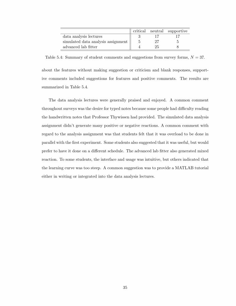
critical neutral supportivedata analysis lectures 3 17 17simulated data analysis assignment 5 27 5advanced lab fitter 4 25 8

Table 5.4: Summary of student comments and suggestions from survey forms, N = 37.

about the features without making suggestion or criticism and blank responses, support-

ive comments included suggestions for features and positive comments. The results are

summarized in Table 5.4.

The data analysis lectures were generally praised and enjoyed. A common comment

throughout surveys was the desire for typed notes because some people had difficulty reading

the handwritten notes that Professor Thywissen had provided. The simulated data analysis

assignment didn’t generate many positive or negative reactions. A common comment with

regard to the analysis assignment was that students felt that it was overload to be done in

parallel with the first experiment. Some students also suggested that it was useful, but would

prefer to have it done on a different schedule. The advanced lab fitter also generated mixed

reaction. To some students, the interface and usage was intuitive, but others indicated that

the learning curve was too steep. A common suggestion was to provide a MATLAB tutorial

either in writing or integrated into the data analysis lectures.

35

Chapter 6

Conclusions

The addition of a data analysis component to the advanced physics laboratory has been

beneficial and has helped to address a gap in content that laboratory students lack. However,

there are limitations to the impact of the proposed and implemented set of curriculum

additions.

The data analysis lectures were generally well received. Students strongly agreed that

the data analysis lectures were valuable, and had mostly supportive and positive comments

about its implementation. The application of this material was found to have significant

value to the performance of students. All grades, including the simulated data analysis

assignment and the two experiment grades were moderately correlated with students’ degree

of application of the lecture material.

The simulated data analysis assignment met a mixed reaction. Based on survey re-

sponses, students felt that it was equally valuable, but had additional criticisms of its

implementation. It is valuable because it reinforces the application of lecture material in a

fairly realistic example. However, the assignment was not found to have significant impact

on student performance nor any correlation to student performance, other than assignment

grade to experiment grade. This suggests that while the assignment may be useful in theory,

in practice it ended up being somewhat cumbersome.

36

A positive outcome from the assignment of the simulated data analysis assignment was

the adoption of the advanced lab fitter. Students who used the fitter were able to complete

the simulated data assignment with ease, and may students who used the advanced lab

fitter in their assignment continued to use it in their laboratory work. The simulated data

analysis assignment could be used as a tutorial exercise for the advanced lab fitter, since

the solutions are generating using the same code. Overall, the introduction of formal data

analysis instruction had a positive outcome, although not yielding considerable improvement

in student performance.

Recommendations for revisions to the data analysis curriculum are outlined in the next

chapter.

37

Chapter 7

Further work

7.1 Additional changes to curriculum

The results of this study have suggested that the value of the simulated data analysis as-

signment is limited. However, as a springboard to using the MATLAB-based advanced lab

fitter, it has proved to be useful. The simulated data analysis assignment could be given as

a tutorial for the advanced lab fitter by making its usage mandatory. A short MATLAB tu-

torial and fitter walkthrough could be provided with the assignments to encourage students

to use the tool.

The data analysis lectures could be expanded to cover a greater number of topics and

made separate from the experiments. The idea of separating the data analysis component

from the experimental work entirely by reserving the first week of the semester has been

brought up in discussions with the course coordinator. This suggestion would facilitate

expanded lectures and additional tutorial on the usage of the data analysis environment.

38

7.2 Continuing analysis of curriculum effectiveness

If the data analysis lectures and simulated data analysis assignment are made permanent

parts of the advanced physics laboratory, then there must be continued analysis on the

effectiveness of the curriculum. In particular, questions of student perceptions of value,

adoption rate, approval of tools, and changes in grade performance should be examined in

the longer term.

7.3 Fitter improvements and supplemental material

Student suggestions have been useful for identifying possible expansions of functionality for

future versions of the tool. Relatively simple additions to the tool-set could include a 3-D

surface fitting toolkit, which can actually run on the existing fitting engine with changes

only to the metric wrapper functions.

MATLAB remains an environment with a steep learning curve. However, its ubiquity

in scientific and engineering research warrants its instruction. In addition, the availability

of a better tool begs its usage. The addition of a MATLAB tutorial and fitter walkthrough

to the simulated data assignment would greatly reduce the pain of learning how to use

MATLAB. The installation of the fitter on the Nortel lab computers using the student

accounts proved to be quite tricky. Pre-installation could also minimize headaches. A side

benefit of moving to a single fitting solution is that students will have more opportunity

to help each other within the lab. With a cornucopia of different data analysis tools and

packages, each person has the responsibility of learning and maintaining their own tools.

However, with a environment and tool, students will be able to assist each other with their

analyses.

39

References

[1] Philip R. Bevington and D. Keith Robinson. Data reduction and error analysis for the

physical sciences. McGraw-Hill, third edition, 2003.

[2] John R. de Bruyn, J. K. C. Lewis, M. R. Morrow, S. P. Norris, N. H. Rich, J. P. White-

head, and M. D. Whitmore. Expanding the role of computers in physics education: A

computer-based first-year course on computational physics and data analysis. Canadian

Journal of Physics, 80, 2002.

[3] John Dewey. Democracy and education. Free Press, 1916.

[4] Robert Ehrlich. How do we know if we are doing a good job in physics teaching?

American Journal of Physics, 70(1), January 2002.

[5] Andrew Elby. Helping physics students learn how to learn. American Journal of Physics

Supplement, 69(7), July 2001.

[6] Edward F. Redish. Millikan lecture 1998: Building a science of teaching physics. Amer-

ican Journal of Physics, 67(7), July 1998.

[7] Edward F. Redish, Jeffery M. Saul, and Richard N. Steinberg. Student expectations in

introductory physics. American Journal of Physics, 66(3), March 1998.

40

Appendix A

Advanced Lab Fitter

A.1 Functional description

The following material has been adapted from the Advanced Lab Fitter manual.

A.1.1 Introduction and Principles of Operation

The fitter operates in MATLAB and has a graphical user interface to shield the user fromthe tedium of handling command line options. The fitter works under the principle that aset of measurements should be organized by variable. So, if we take a set of measurements oftemperature and voltage, the voltage measurements can be given a name, say volt and thetemperature measurement can be given a name, say temp. This is opposed to an analysissystem that works under the principle that measurements should be organized by datapoint.

Every set of data must be represented in the workspace as an N × 2 matrix. Byconvention, the first column is always the measurement and the second column is alwaysthe uncertainty. This is consistent with the idea that a measurement is not meaningfulwithout an uncertainty. Another note is that to be able to fit or plot two variables, theymust have the same number of rows.

So, suppose we perform an experiment and collect 3 data points of temperature andvoltage, (280± 1 K,−0.45± 0.03 mV), (290± 1 K, 0.04± 0.06 mV), and (300± 1 K, 0.66±0.07 mV).

These data should be defined in your workspace with two matrices,

temp =

280 1290 1300 1

and volt =

−0.45 0.030.04 0.060.66 0.07

41

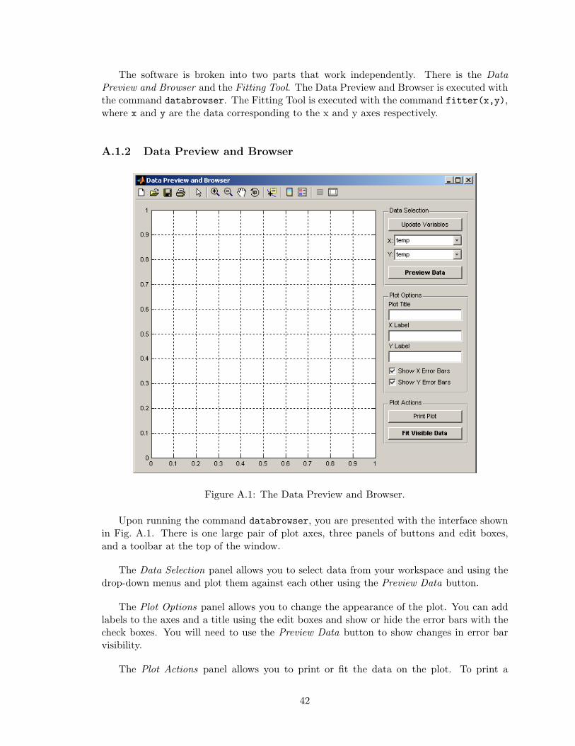
The software is broken into two parts that work independently. There is the DataPreview and Browser and the Fitting Tool. The Data Preview and Browser is executed withthe command databrowser. The Fitting Tool is executed with the command fitter(x,y),where x and y are the data corresponding to the x and y axes respectively.

A.1.2 Data Preview and Browser

Figure A.1: The Data Preview and Browser.

Upon running the command databrowser, you are presented with the interface shownin Fig. A.1. There is one large pair of plot axes, three panels of buttons and edit boxes,and a toolbar at the top of the window.

The Data Selection panel allows you to select data from your workspace and using thedrop-down menus and plot them against each other using the Preview Data button.

The Plot Options panel allows you to change the appearance of the plot. You can addlabels to the axes and a title using the edit boxes and show or hide the error bars with thecheck boxes. You will need to use the Preview Data button to show changes in error barvisibility.

The Plot Actions panel allows you to print or fit the data on the plot. To print a

42

formatted plot which will fit nicely into a standard black lab book, click the Print Plotbutton. Do not use the print button in the toolbar. You must have a preview of your datavisible to print. To fit all of the data points that are visible within the limits of the previewplot, click the Fit Visible Data button and an instance of the Fitting Tool will be openedwith the visible data.

Data can be selected for fitting by changing the view of the data. This can be accom-plished by using the zoom and pan tools from the toolbar. The zoom in tool is activated byclicking on the button with the positive magnifying glass. The zoom out tool is activatedby clicking the button with the negative magnifying glass. pan tool is activated by clickingthe button with the white hand. All tools can be deactivated by clicking on their respectivebuttons a second time (they toggle). They are used by clicking and dragging on the plot.

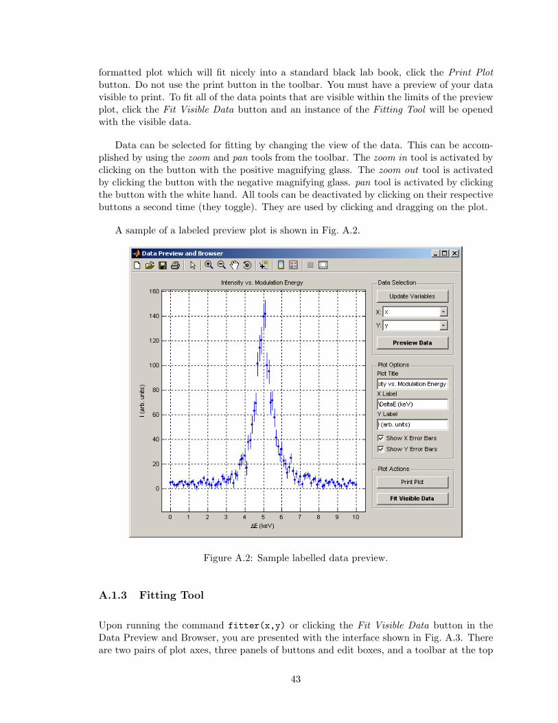
A sample of a labeled preview plot is shown in Fig. A.2.

Figure A.2: Sample labelled data preview.

A.1.3 Fitting Tool

Upon running the command fitter(x,y) or clicking the Fit Visible Data button in theData Preview and Browser, you are presented with the interface shown in Fig. A.3. Thereare two pairs of plot axes, three panels of buttons and edit boxes, and a toolbar at the top

43

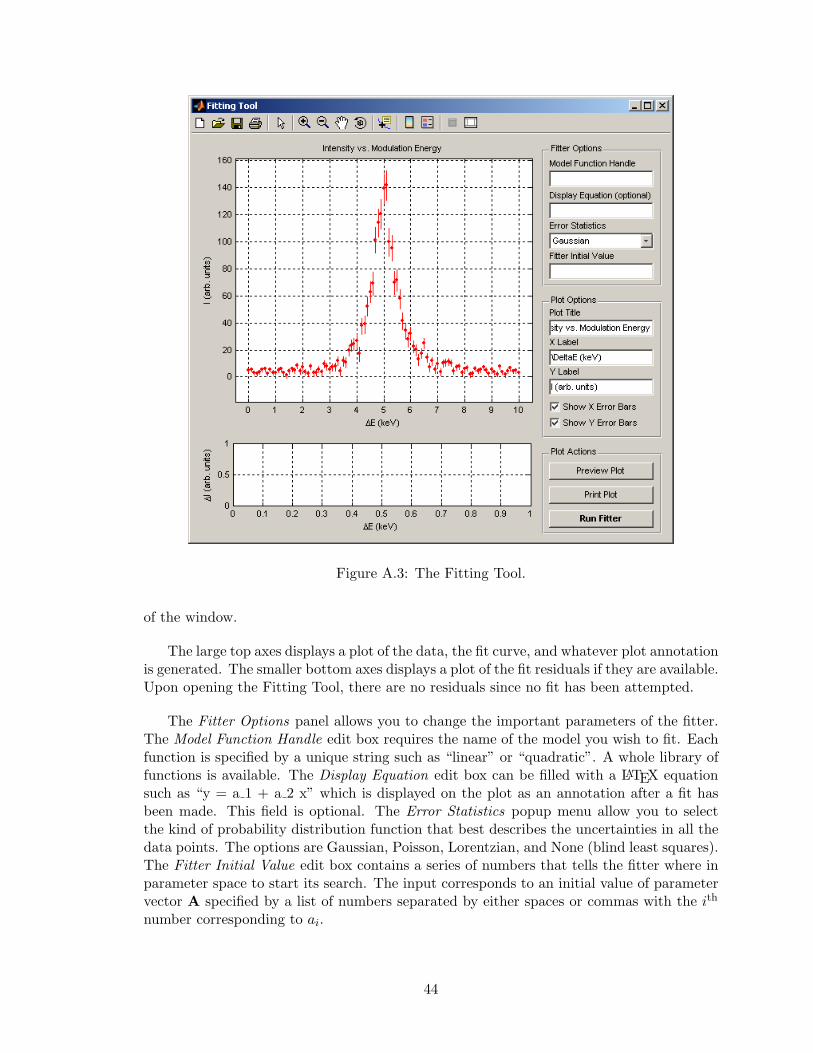
Figure A.3: The Fitting Tool.

of the window.

The large top axes displays a plot of the data, the fit curve, and whatever plot annotationis generated. The smaller bottom axes displays a plot of the fit residuals if they are available.Upon opening the Fitting Tool, there are no residuals since no fit has been attempted.

The Fitter Options panel allows you to change the important parameters of the fitter.The Model Function Handle edit box requires the name of the model you wish to fit. Eachfunction is specified by a unique string such as “linear” or “quadratic”. A whole library offunctions is available. The Display Equation edit box can be filled with a LATEX equationsuch as “y = a 1 + a 2 x” which is displayed on the plot as an annotation after a fit hasbeen made. This field is optional. The Error Statistics popup menu allow you to selectthe kind of probability distribution function that best describes the uncertainties in all thedata points. The options are Gaussian, Poisson, Lorentzian, and None (blind least squares).The Fitter Initial Value edit box contains a series of numbers that tells the fitter where inparameter space to start its search. The input corresponds to an initial value of parametervector A specified by a list of numbers separated by either spaces or commas with the ith

number corresponding to ai.

44

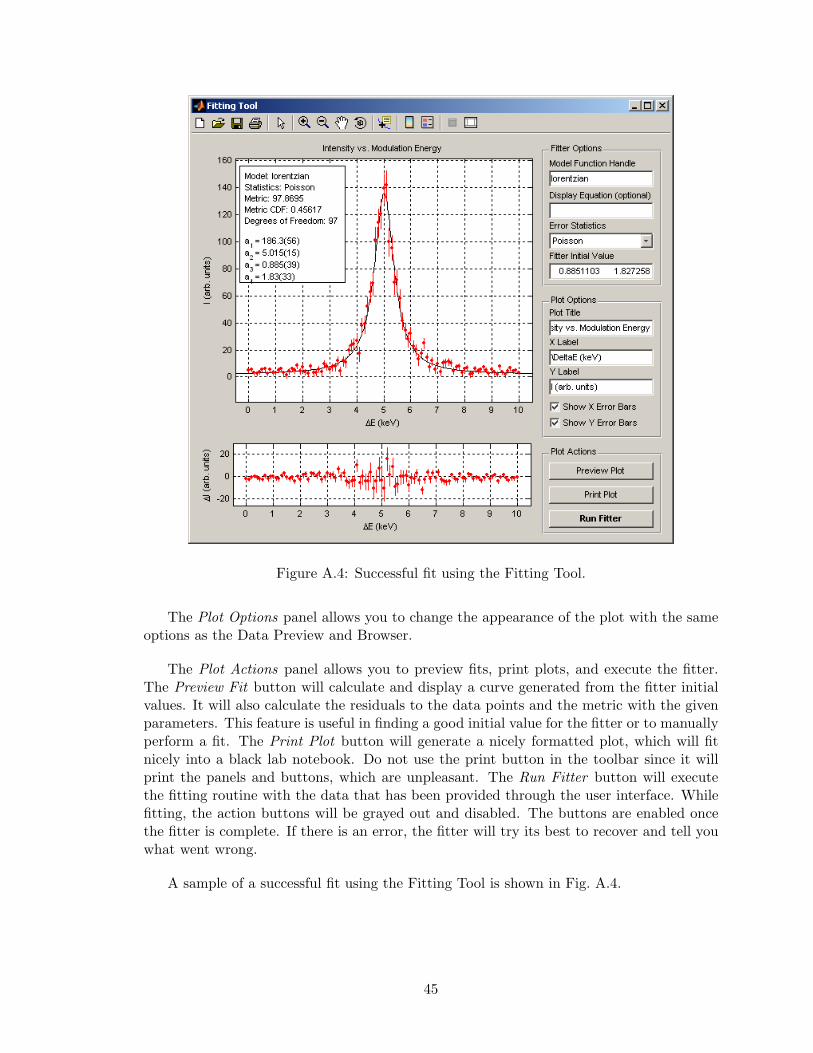
Figure A.4: Successful fit using the Fitting Tool.

The Plot Options panel allows you to change the appearance of the plot with the sameoptions as the Data Preview and Browser.

The Plot Actions panel allows you to preview fits, print plots, and execute the fitter.The Preview Fit button will calculate and display a curve generated from the fitter initialvalues. It will also calculate the residuals to the data points and the metric with the givenparameters. This feature is useful in finding a good initial value for the fitter or to manuallyperform a fit. The Print Plot button will generate a nicely formatted plot, which will fitnicely into a black lab notebook. Do not use the print button in the toolbar since it willprint the panels and buttons, which are unpleasant. The Run Fitter button will executethe fitting routine with the data that has been provided through the user interface. Whilefitting, the action buttons will be grayed out and disabled. The buttons are enabled oncethe fitter is complete. If there is an error, the fitter will try its best to recover and tell youwhat went wrong.

A sample of a successful fit using the Fitting Tool is shown in Fig. A.4.

45

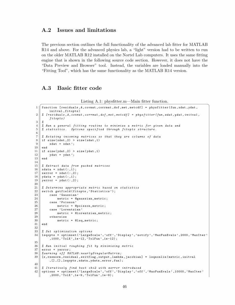
A.2 Issues and limitations

The previous section outlines the full functionality of the advanced lab fitter for MATLABR14 and above. For the advanced physics lab, a “light” version had to be written to runon the older MATLAB R12 installed on the Nortel Lab computers. It uses the same fittingengine that is shown in the following source code section. However, it does not have the“Data Preview and Browser” tool. Instead, the variables are loaded manually into the“Fitting Tool”, which has the same functionality as the MATLAB R14 version.

A.3 Basic fitter code

Listing A.1: physfitter.m—Main fitter function.¨ ¥1 function [residuals ,A,covmat ,corrmat ,dof ,met ,metcdf] = physfitter(fun ,xdat ,ydat ,

initval ,fitopts)

2 % [residuals ,A,covmat ,corrmat ,dof ,met ,metcdf] = physfitter (fun ,xdat ,ydat ,initval ,

fitopts)

3 %

4 % Run a general fitting routine to minimize a metric for given data and

5 % statistics . Options specified through fitopts structure.

67 % Rotating incoming matrices so that they are columns of data

8 if size(xdat ,2) > size(xdat ,1)

9 xdat = xdat ’;

10 end

11 if size(ydat ,2) > size(ydat ,1)

12 ydat = ydat ’;

13 end

1415 % Extract data from packed matrices

16 xdata = xdat (:,1);

17 xerror = xdat (:,2);

18 ydata = ydat (:,1);

19 yerror = ydat (:,2);

2021 % Determine appropriate metric based on statistics

22 switch getfield(fitopts ,’Statistics ’);

23 case ’Gaussian ’

24 metric = @gaussian_metric;

25 case ’Poisson ’

26 metric = @poisson_metric;

27 case ’Lorentzian ’

28 metric = @lorentzian_metric;

29 otherwise

30 metric = @lsq_metric;

31 end

3233 % Set optimization options

34 lsqopts = optimset(’LargeScale ’,’off’,’Display ’,’notify ’,’MaxFunEvals ’ ,2000,’MaxIter ’

,1000,’TolX’,1e-12,’TolFun ’,1e-12);

3536 % Run initial roughing fit by minimizing metric

37 error = yerror;

38 %warning off MATLAB: nearlySingularMatrix ;

39 [x,resnorm ,residual ,exitflag ,output ,lambda ,jacobian] = lsqnonlin(metric ,initval

,[],[],lsqopts ,xdata ,ydata ,error ,fun);

4041 % Iteratively find best chi2 with xerror introduced

42 options = optimset(’LargeScale ’,’off’,’Display ’,’off’,’MaxFunEvals ’ ,10000,’MaxIter ’

,2000,’TolX’,1e-9,’TolFun ’,1e-9);

46

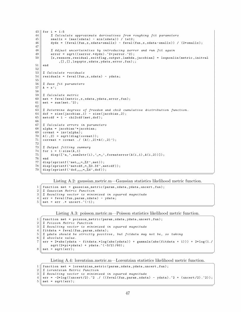
43 for i = 1:5

44 % Calculate approximate derivatives from roughing fit parameters

45 smallx = (max(xdata) - min(xdata)) / 1e12;

46 dydx = (feval(fun ,x,xdata+smallx) - feval(fun ,x,xdata -smallx)) / (2* smallx);

4748 % Adjust uncertainties by introducing xerror and run fit again

49 error = sqrt(( xerror .*dydx).^2+ yerror .^2);

50 [x,resnorm ,residual ,exitflag ,output ,lambda ,jacobian] = lsqnonlin(metric ,initval

,[],[],lsqopts ,xdata ,ydata ,error ,fun);;

51 end

5253 % Calculate residuals

54 residuals = feval(fun ,x,xdata) - ydata;

5556 % Save fit parameters

57 A = x’;

5859 % Calculate metric

60 met = feval(metric ,x,xdata ,ydata ,error ,fun);

61 met = sum(met .^2);

6263 % Determine degrees of freedom and chi2 cumulative distribution function.

64 dof = size(jacobian ,1) - size(jacobian ,2);

65 metcdf = 1 - chi2cdf(met ,dof);

6667 % Calculate errors in parameters

68 alpha = jacobian ’* jacobian;

69 covmat = inv(alpha);

70 A(:,2) = sqrt(diag(covmat));

71 corrmat = covmat ./ (A(:,2)*A(:,2) ’);

7273 % Output fitting summary

74 for i = 1:size(A,1)

75 disp([’a_’,num2str(i),’Ã=Ã’,formaterror(A(i,1),A(i,2))]);

76 end

77 disp(sprintf(’metÃÃ=Ã%f’,met));

78 disp(sprintf(’metcdfÃ=Ã%0.3f’,metcdf));

79 disp(sprintf(’dofÃÃÃ=Ã%d’,dof));­§ ¦

Listing A.2: gaussian metric.m—Gaussian statistics likelihood metric function.¨ ¥1 function met = gaussian_metric(param ,xdata ,ydata ,uncert ,fun);

2 % Gaussian Metric Function

3 % Resulting vector is minimized in squared magnitude

4 err = feval(fun ,param ,xdata) - ydata;

5 met = err .* uncert .^( -1);­§ ¦

Listing A.3: poisson metric.m—Poisson statistics likelihood metric function.¨ ¥1 function met = poisson_metric(param ,xdata ,ydata ,uncert ,fun);

2 % Poisson Metric Function

3 % Resulting vector is minimized in squared magnitude

4 fitdata = feval(fun ,param ,xdata);

5 % ydata should be strictly positive , but fitdata may not be , so taking

6 % absolute value.

7 err = 2*abs(ydata - fitdata .*log(abs(ydata)) + gammaln(abs(fitdata + 1))) + 2*log (1./

sqrt (2*pi*ydata) + ydata .^( -3/2) /60);

8 met = sqrt(err);­§ ¦

Listing A.4: lorentzian metric.m—Lorentzian statistics likelihood metric function.¨ ¥1 function met = lorentzian_metric(param ,xdata ,ydata ,uncert ,fun);

2 % Lorentzian Metric Function

3 % Resulting vector is minimized in squared magnitude

4 err = -2*log(( uncert /2).^2 ./ ((feval(fun ,param ,xdata) - ydata).^2 + (uncert /2) .^2));

5 met = sqrt(err);­§ ¦

47

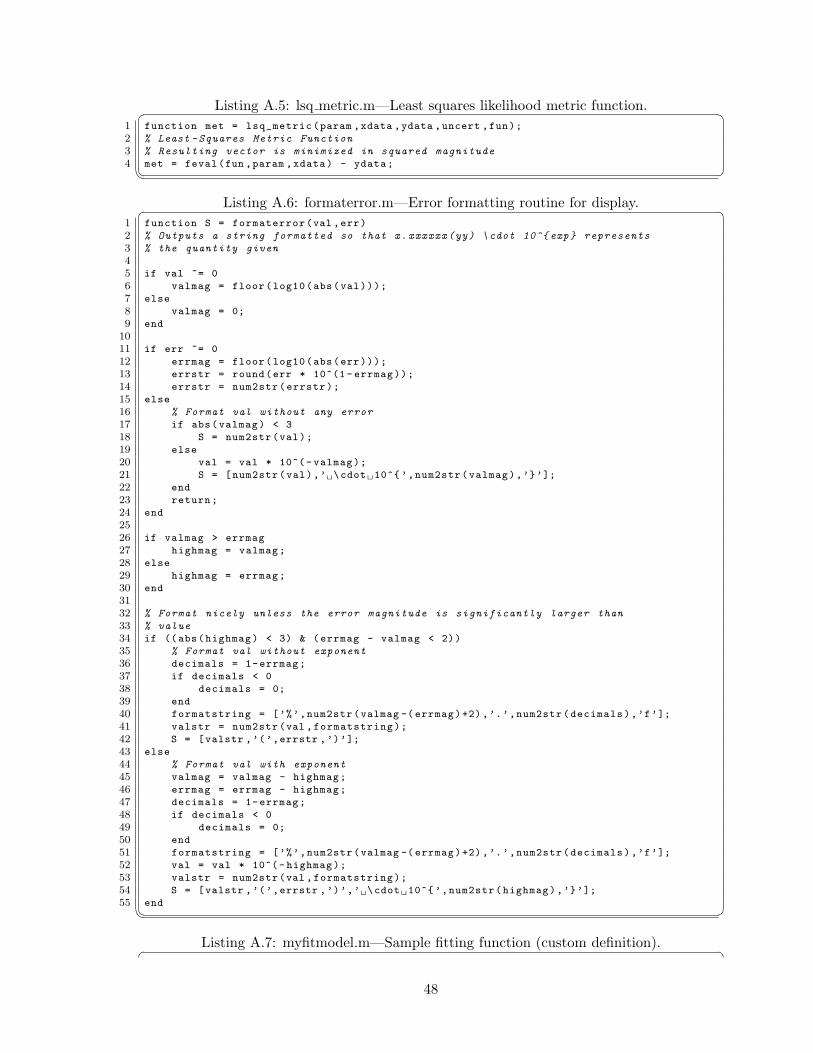
Listing A.5: lsq metric.m—Least squares likelihood metric function.¨ ¥1 function met = lsq_metric(param ,xdata ,ydata ,uncert ,fun);

2 % Least -Squares Metric Function

3 % Resulting vector is minimized in squared magnitude

4 met = feval(fun ,param ,xdata) - ydata;­§ ¦

Listing A.6: formaterror.m—Error formatting routine for display.¨ ¥1 function S = formaterror(val ,err)

2 % Outputs a string formatted so that x.xxxxxx(yy) \cdot 10^{ exp} represents

3 % the quantity given

45 if val ~= 0

6 valmag = floor(log10(abs(val)));

7 else

8 valmag = 0;

9 end

1011 if err ~= 0

12 errmag = floor(log10(abs(err)));

13 errstr = round(err * 10^(1- errmag));

14 errstr = num2str(errstr);

15 else

16 % Format val without any error

17 if abs(valmag) < 3

18 S = num2str(val);

19 else

20 val = val * 10^(- valmag);

21 S = [num2str(val),’Ã\cdotÃ10^{’,num2str(valmag),’}’];

22 end

23 return;

24 end

2526 if valmag > errmag

27 highmag = valmag;

28 else

29 highmag = errmag;

30 end

3132 % Format nicely unless the error magnitude is significantly larger than

33 % value

34 if ((abs(highmag) < 3) & (errmag - valmag < 2))

35 % Format val without exponent

36 decimals = 1-errmag;

37 if decimals < 0

38 decimals = 0;

39 end

40 formatstring = [’%’,num2str(valmag -( errmag)+2),’.’,num2str(decimals),’f’];

41 valstr = num2str(val ,formatstring);

42 S = [valstr ,’(’,errstr ,’)’];

43 else

44 % Format val with exponent

45 valmag = valmag - highmag;

46 errmag = errmag - highmag;

47 decimals = 1-errmag;

48 if decimals < 0

49 decimals = 0;

50 end

51 formatstring = [’%’,num2str(valmag -( errmag)+2),’.’,num2str(decimals),’f’];

52 val = val * 10^(- highmag);

53 valstr = num2str(val ,formatstring);

54 S = [valstr ,’(’,errstr ,’)’,’Ã\cdotÃ10^{’,num2str(highmag),’}’];

55 end­§ ¦

Listing A.7: myfitmodel.m—Sample fitting function (custom definition).¨ ¥

48

1 function y = myfitmodel(a,x)

2 y = a(1) * x.^2 .* sin(a(2)*x) + a(3);­§ ¦

49

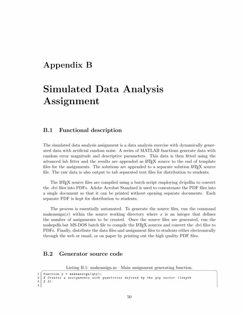
Appendix B

Simulated Data AnalysisAssignment

B.1 Functional description

The simulated data analysis assignment is a data analysis exercise with dynamically gener-ated data with artificial random noise. A series of MATLAB functions generate data withrandom error magnitude and descriptive parameters. This data is then fitted using theadvanced lab fitter and the results are appended as LATEX source to the end of templatefiles for the assignments. The solutions are appended to a separate solution LATEX sourcefile. The raw data is also output to tab separated text files for distribution to students.

The LATEX source files are compiled using a batch script employing dvipdfm to convertthe .dvi files into PDFs. Adobe Acrobat Standard is used to concatenate the PDF files intoa single document so that it can be printed without opening separate documents. Eachseparate PDF is kept for distribution to students.

The process is essentially automated. To generate the source files, run the commandmakeassign(x) within the source working directory where x is an integer that definesthe number of assignments to be created. Once the source files are generated, run themakepdfs.bat MS-DOS batch file to compile the LATEX sources and convert the .dvi files toPDFs. Finally, distribute the data files and assignment files to students either electronicallythrough the web or email, or on paper by printing out the high quality PDF files.

B.2 Generator source code

Listing B.1: makeassign.m—Main assignment generating function.¨ ¥1 function y = makeassign(qty);

2 % Creates a assignments with quantities defined by the qty vector (length

3 % 3).

4

50

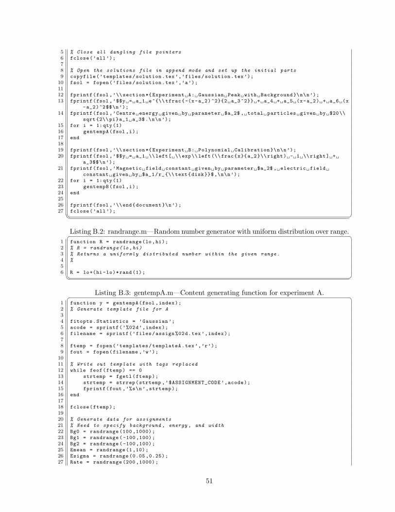
5 % Close all dangling file pointers

6 fclose(’all’);

78 % Open the solutions file in append mode and set up the initial parts

9 copyfile(’templates/solution.tex’,’files/solution.tex’);

10 fsol = fopen(’files/solution.tex’,’a’);

1112 fprintf(fsol ,’\\ section *{ ExperimentÃA:ÃGaussianÃPeakÃwithÃBackground }\n\n’);

13 fprintf(fsol ,’$$yÃ=Ãa_1Ãe^{\\ tfrac{-(x-a_2)^2}{2Ãa_3 ^2}}Ã+Ãa_4Ã+Ãa_5Ã(x-a_2)Ã+Ãa_6Ã(x

-a_2)^2$$\n’);

14 fprintf(fsol ,’CentreÃenergyÃgivenÃbyÃparameterÃ$a_2$ ,ÃtotalÃparticlesÃgivenÃbyÃ$20\\

sqrt {2\\pi}a_1Ãa_3$.\n\n’);

15 for i = 1:qty(1)

16 gentempA(fsol ,i);

17 end

1819 fprintf(fsol ,’\\ section *{ ExperimentÃB:ÃPolynomialÃCalibration }\n\n’);

20 fprintf(fsol ,’$$yÃ=Ãa_1Ã\\left[Ã\\exp\\left (\\ frac{x}{a_2}\\ right)Ã-Ã1Ã\\right]Ã+Ã

a_3$$\n’);

21 fprintf(fsol ,’MagneticÃfieldÃconstantÃgivenÃbyÃparameterÃ$a_2$ ,ÃelectricÃfieldÃ

constantÃgivenÃbyÃ$a_1/r_{\\ text{disk}}$,\n\n’);

22 for i = 1:qty(1)

23 gentempB(fsol ,i);

24 end

2526 fprintf(fsol ,’\\end{document }\n’);

27 fclose(’all’);­§ ¦

Listing B.2: randrange.m—Random number generator with uniform distribution over range.¨ ¥1 function R = randrange(lo ,hi);

2 % R = randrange(lo ,hi)

3 % Returns a uniformly distributed number within the given range.

4 %

56 R = lo+(hi-lo)*rand (1);

­§ ¦

Listing B.3: gentempA.m—Content generating function for experiment A.¨ ¥1 function y = gentempA(fsol ,index);

2 % Generate template file for A

34 fitopts.Statistics = ’Gaussian ’;

5 acode = sprintf(’%02d’,index);

6 filename = sprintf(’files/assign %02d.tex’,index);

78 ftemp = fopen(’templates/templateA.tex’,’r’);

9 fout = fopen(filename ,’w’);

1011 % Write out template with tags replaced

12 while feof(ftemp) == 0

13 strtemp = fgetl(ftemp);

14 strtemp = strrep(strtemp ,’$ASSIGNMENT_CODE ’,acode);

15 fprintf(fout ,’%s\n’,strtemp);

16 end

1718 fclose(ftemp);

1920 % Generate data for assignments

21 % Need to specify background , energy , and width

22 Bg0 = randrange (100 ,1000);

23 Bg1 = randrange ( -100 ,100);

24 Bg2 = randrange ( -100 ,100);

25 Emean = randrange (1,10);

26 Esigma = randrange (0.05 ,0.25);

27 Rate = randrange (200 ,1000);

51

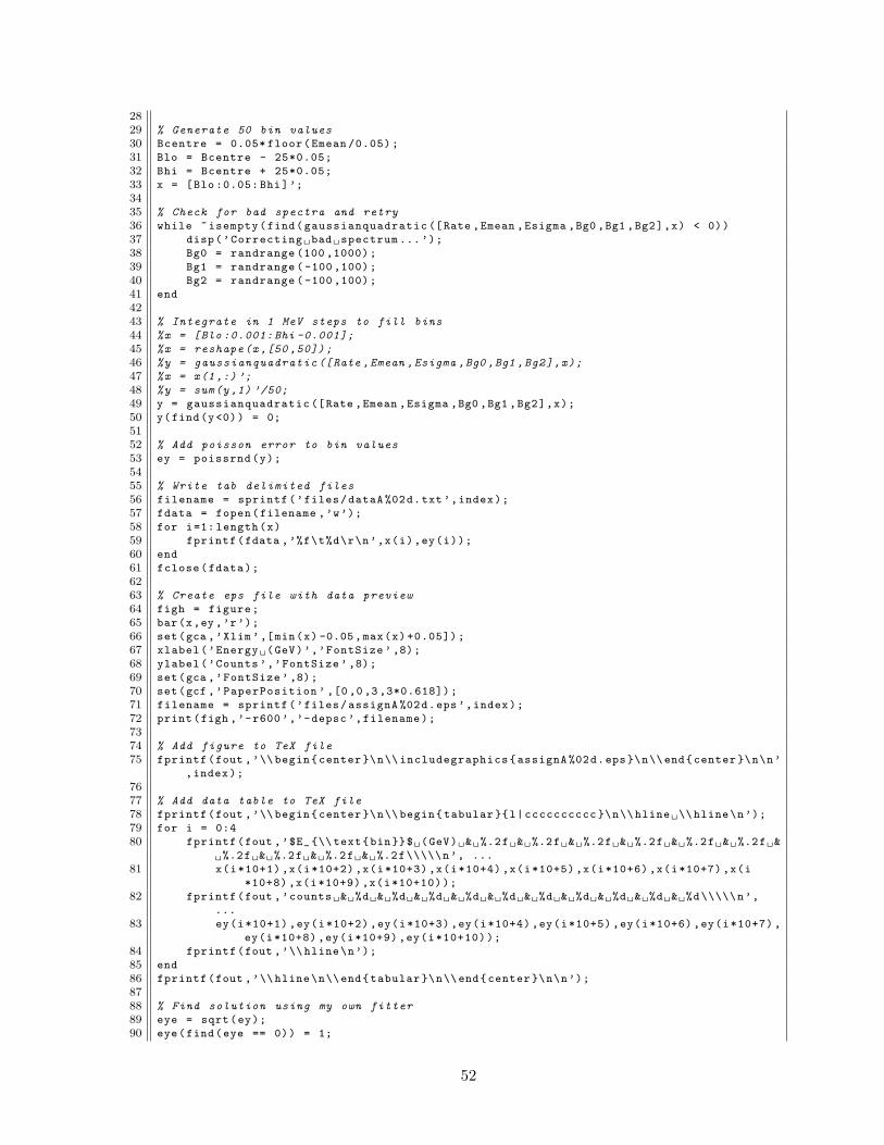
2829 % Generate 50 bin values

30 Bcentre = 0.05* floor(Emean /0.05);

31 Blo = Bcentre - 25*0.05;

32 Bhi = Bcentre + 25*0.05;

33 x = [Blo :0.05: Bhi]’;

3435 % Check for bad spectra and retry

36 while ~isempty(find(gaussianquadratic ([Rate ,Emean ,Esigma ,Bg0 ,Bg1 ,Bg2],x) < 0))

37 disp(’CorrectingÃbadÃspectrum ...’);

38 Bg0 = randrange (100 ,1000);

39 Bg1 = randrange ( -100 ,100);

40 Bg2 = randrange ( -100 ,100);

41 end

4243 % Integrate in 1 MeV steps to fill bins

44 %x = [Blo :0.001: Bhi -0.001];

45 %x = reshape(x ,[50 ,50]);

46 %y = gaussianquadratic ([Rate ,Emean ,Esigma ,Bg0 ,Bg1 ,Bg2],x);

47 %x = x(1 ,:) ’;

48 %y = sum(y ,1) ’/50;

49 y = gaussianquadratic ([Rate ,Emean ,Esigma ,Bg0 ,Bg1 ,Bg2],x);

50 y(find(y<0)) = 0;

5152 % Add poisson error to bin values

53 ey = poissrnd(y);

5455 % Write tab delimited files

56 filename = sprintf(’files/dataA %02d.txt’,index);

57 fdata = fopen(filename ,’w’);

58 for i=1: length(x)

59 fprintf(fdata ,’%f\t%d\r\n’,x(i),ey(i));

60 end

61 fclose(fdata);

6263 % Create eps file with data preview

64 figh = figure;

65 bar(x,ey,’r’);

66 set(gca ,’Xlim’,[min(x) -0.05,max(x)+0.05]);

67 xlabel(’EnergyÃ(GeV)’,’FontSize ’ ,8);

68 ylabel(’Counts ’,’FontSize ’ ,8);

69 set(gca ,’FontSize ’ ,8);

70 set(gcf ,’PaperPosition ’ ,[0 ,0 ,3 ,3*0.618]);

71 filename = sprintf(’files/assignA %02d.eps’,index);

72 print(figh ,’-r600’,’-depsc’,filename);

7374 % Add figure to TeX file

75 fprintf(fout ,’\\begin{center }\n\\ includegraphics{assignA %02d.eps}\n\\end{center }\n\n’

,index);

7677 % Add data table to TeX file

78 fprintf(fout ,’\\begin{center }\n\\ begin{tabular }{l|cccccccccc }\n\\hlineÃ\\hline\n’);

79 for i = 0:4

80 fprintf(fout ,’$E_ {\\ text{bin}}$Ã(GeV)Ã&Ã%.2fÃ&Ã%.2fÃ&Ã%.2fÃ&Ã%.2fÃ&Ã%.2fÃ&Ã%.2fÃ&

Ã%.2fÃ&Ã%.2fÃ&Ã%.2fÃ&Ã%.2f\\\\\n’, ...

81 x(i*10+1) ,x(i*10+2) ,x(i*10+3) ,x(i*10+4) ,x(i*10+5) ,x(i*10+6) ,x(i*10+7) ,x(i

*10+8) ,x(i*10+9) ,x(i*10+10));

82 fprintf(fout ,’countsÃ&Ã%dÃ&Ã%dÃ&Ã%dÃ&Ã%dÃ&Ã%dÃ&Ã%dÃ&Ã%dÃ&Ã%dÃ&Ã%dÃ&Ã%d\\\\\n’,

...

83 ey(i*10+1) ,ey(i*10+2) ,ey(i*10+3) ,ey(i*10+4) ,ey(i*10+5) ,ey(i*10+6) ,ey(i*10+7) ,

ey(i*10+8) ,ey(i*10+9) ,ey(i*10+10));

84 fprintf(fout ,’\\hline\n’);

85 end

86 fprintf(fout ,’\\hline\n\\end{tabular }\n\\end{center }\n\n’);

8788 % Find solution using my own fitter

89 eye = sqrt(ey);

90 eye(find(eye == 0)) = 1;

52

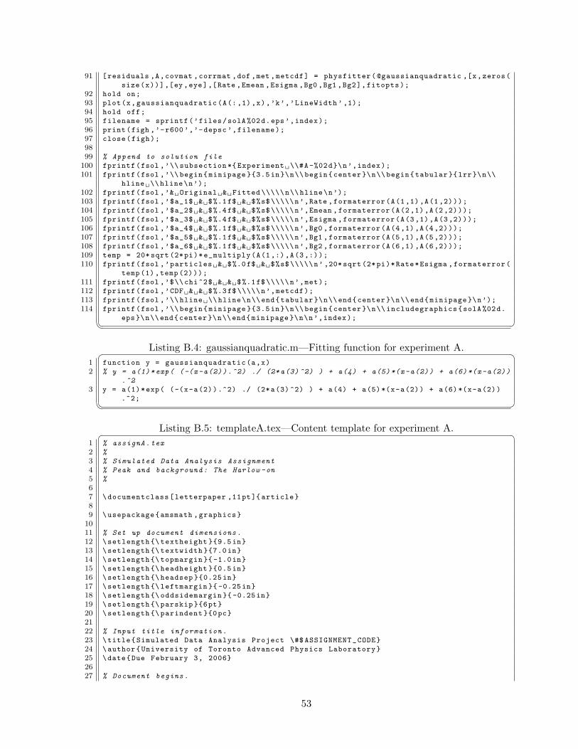
91 [residuals ,A,covmat ,corrmat ,dof ,met ,metcdf] = physfitter(@gaussianquadratic ,[x,zeros(

size(x))],[ey ,eye],[Rate ,Emean ,Esigma ,Bg0 ,Bg1 ,Bg2],fitopts);

92 hold on;

93 plot(x,gaussianquadratic(A(:,1),x),’k’,’LineWidth ’ ,1);

94 hold off;

95 filename = sprintf(’files/solA %02d.eps’,index);

96 print(figh ,’-r600’,’-depsc’,filename);

97 close(figh);

9899 % Append to solution file

100 fprintf(fsol ,’\\ subsection *{ ExperimentÃ\\#A-%02d}\n’,index);

101 fprintf(fsol ,’\\begin{minipage }{3.5in}\n\\begin{center }\n\\begin{tabular }{lrr}\n\\

hlineÃ\\hline\n’);

102 fprintf(fsol ,’&ÃOriginalÃ&ÃFitted \\\\\n\\ hline\n’);

103 fprintf(fsol ,’$a_1$Ã&Ã$%.1f$Ã&Ã$%s$\\\\\n’,Rate ,formaterror(A(1,1),A(1,2)));

104 fprintf(fsol ,’$a_2$Ã&Ã$%.4f$Ã&Ã$%s$\\\\\n’,Emean ,formaterror(A(2,1),A(2,2)));

105 fprintf(fsol ,’$a_3$Ã&Ã$%.4f$Ã&Ã$%s$\\\\\n’,Esigma ,formaterror(A(3,1),A(3,2)));

106 fprintf(fsol ,’$a_4$Ã&Ã$%.1f$Ã&Ã$%s$\\\\\n’,Bg0 ,formaterror(A(4,1),A(4,2)));

107 fprintf(fsol ,’$a_5$Ã&Ã$%.1f$Ã&Ã$%s$\\\\\n’,Bg1 ,formaterror(A(5,1),A(5,2)));

108 fprintf(fsol ,’$a_6$Ã&Ã$%.1f$Ã&Ã$%s$\\\\\n’,Bg2 ,formaterror(A(6,1),A(6,2)));

109 temp = 20* sqrt (2*pi)*e_multiply(A(1,:),A(3,:));

110 fprintf(fsol ,’particlesÃ&Ã$%.0f$Ã&Ã$%s$\\\\\n’ ,20*sqrt (2*pi)*Rate*Esigma ,formaterror(

temp (1),temp (2)));

111 fprintf(fsol ,’$\\chi^2$Ã&Ã&Ã$%.1f$\\\\\n’,met);

112 fprintf(fsol ,’CDFÃ&Ã&Ã$%.3f$\\\\\n’,metcdf);

113 fprintf(fsol ,’\\hlineÃ\\hline\n\\end{tabular }\n\\end{center }\n\\end{minipage }\n’);

114 fprintf(fsol ,’\\begin{minipage }{3.5in}\n\\begin{center }\n\\ includegraphics{solA %02d.

eps}\n\\end{center }\n\\end{minipage }\n\n’,index);­§ ¦

Listing B.4: gaussianquadratic.m—Fitting function for experiment A.¨ ¥1 function y = gaussianquadratic(a,x)

2 % y = a(1)*exp( (-(x-a(2)).^2) ./ (2*a(3) ^2) ) + a(4) + a(5) *(x-a(2)) + a(6) *(x-a(2))

.^2

3 y = a(1)*exp( (-(x-a(2)).^2) ./ (2*a(3) ^2) ) + a(4) + a(5)*(x-a(2)) + a(6)*(x-a(2))

.^2;­§ ¦

Listing B.5: templateA.tex—Content template for experiment A.¨ ¥1 % assignA.tex

2 %

3 % Simulated Data Analysis Assignment

4 % Peak and background : The Harlow -on

5 %

67 \documentclass[letterpaper ,11pt]{ article}

89 \usepackage{amsmath ,graphics}

1011 % Set up document dimensions .

12 \setlength {\ textheight }{9.5 in}

13 \setlength {\ textwidth }{7.0in}

14 \setlength {\ topmargin }{-1.0in}

15 \setlength {\ headheight }{0.5 in}

16 \setlength {\ headsep }{0.25 in}

17 \setlength {\ leftmargin }{ -0.25in}

18 \setlength {\ oddsidemargin }{ -0.25in}

19 \setlength {\ parskip }{6pt}

20 \setlength {\ parindent }{0pc}

2122 % Input title information .

23 \title{Simulated Data Analysis Project \#$ ASSIGNMENT_CODE}

24 \author{University of Toronto Advanced Physics Laboratory}

25 \date{Due February 3, 2006}

2627 % Document begins.

53

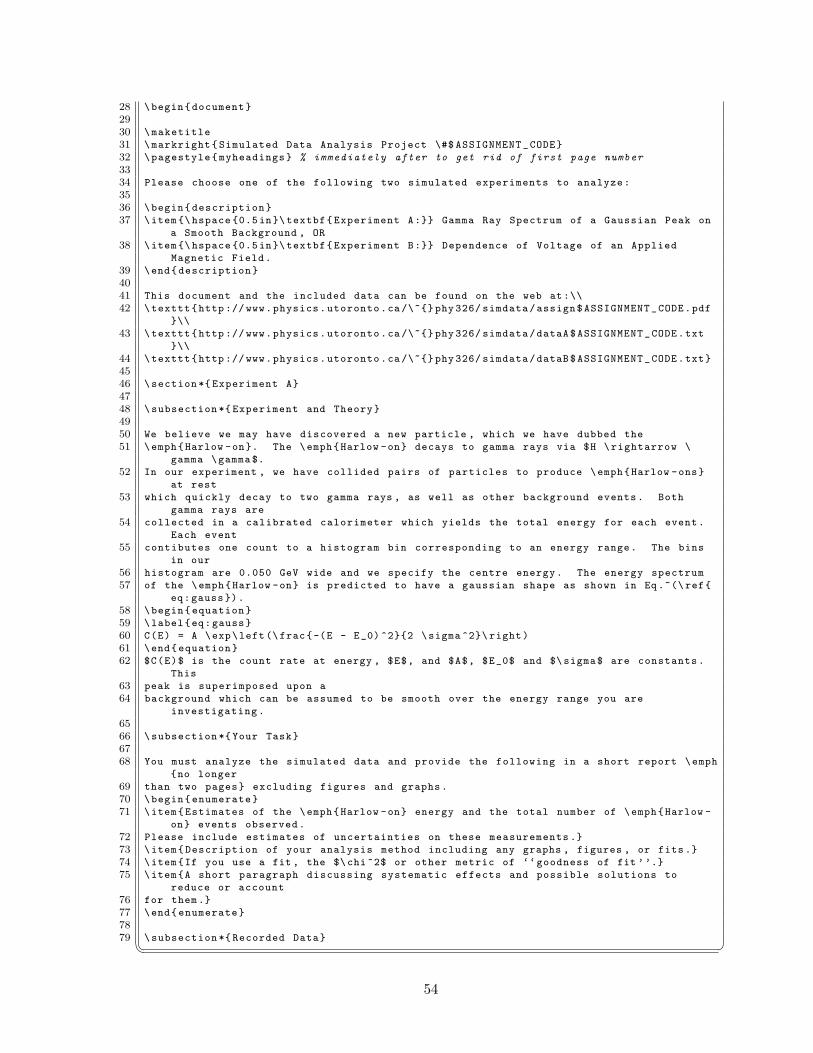
28 \begin{document}

2930 \maketitle

31 \markright{Simulated Data Analysis Project \#$ ASSIGNMENT_CODE}

32 \pagestyle{myheadings} % immediately after to get rid of first page number

3334 Please choose one of the following two simulated experiments to analyze:

3536 \begin{description}

37 \item{\ hspace {0.5in}\ textbf{Experiment A:}} Gamma Ray Spectrum of a Gaussian Peak on

a Smooth Background , OR

38 \item{\ hspace {0.5in}\ textbf{Experiment B:}} Dependence of Voltage of an Applied

Magnetic Field.

39 \end{description}

4041 This document and the included data can be found on the web at:\\

42 \texttt{http ://www.physics.utoronto.ca/\~{} phy 326/ simdata/assign$ASSIGNMENT_CODE.pdf

}\\

43 \texttt{http ://www.physics.utoronto.ca/\~{} phy 326/ simdata/dataA$ASSIGNMENT_CODE.txt

}\\

44 \texttt{http ://www.physics.utoronto.ca/\~{} phy 326/ simdata/dataB$ASSIGNMENT_CODE.txt}

4546 \section *{ Experiment A}

4748 \subsection *{ Experiment and Theory}

4950 We believe we may have discovered a new particle , which we have dubbed the

51 \emph{Harlow -on}. The \emph{Harlow -on} decays to gamma rays via $H \rightarrow \

gamma \gamma $.

52 In our experiment , we have collided pairs of particles to produce \emph{Harlow -ons}

at rest

53 which quickly decay to two gamma rays , as well as other background events. Both

gamma rays are

54 collected in a calibrated calorimeter which yields the total energy for each event.

Each event

55 contibutes one count to a histogram bin corresponding to an energy range. The bins

in our

56 histogram are 0.050 GeV wide and we specify the centre energy. The energy spectrum

57 of the \emph{Harlow -on} is predicted to have a gaussian shape as shown in Eq.~(\ ref{

eq:gauss}).

58 \begin{equation}

59 \label{eq:gauss}

60 C(E) = A \exp\left(\frac{-(E - E_0) ^2}{2 \sigma ^2}\ right)

61 \end{equation}

62 $C(E)$ is the count rate at energy , $E$, and $A$, $E_0$ and $\sigma$ are constants.

This

63 peak is superimposed upon a

64 background which can be assumed to be smooth over the energy range you are

investigating.

6566 \subsection *{Your Task}

6768 You must analyze the simulated data and provide the following in a short report \emph

{no longer

69 than two pages} excluding figures and graphs.

70 \begin{enumerate}

71 \item{Estimates of the \emph{Harlow -on} energy and the total number of \emph{Harlow -

on} events observed.

72 Please include estimates of uncertainties on these measurements .}

73 \item{Description of your analysis method including any graphs , figures , or fits.}

74 \item{If you use a fit , the $\chi ^2$ or other metric of ‘‘goodness of fit ’’.}

75 \item{A short paragraph discussing systematic effects and possible solutions to

reduce or account

76 for them.}

77 \end{enumerate}

7879 \subsection *{ Recorded Data}

­§ ¦

54

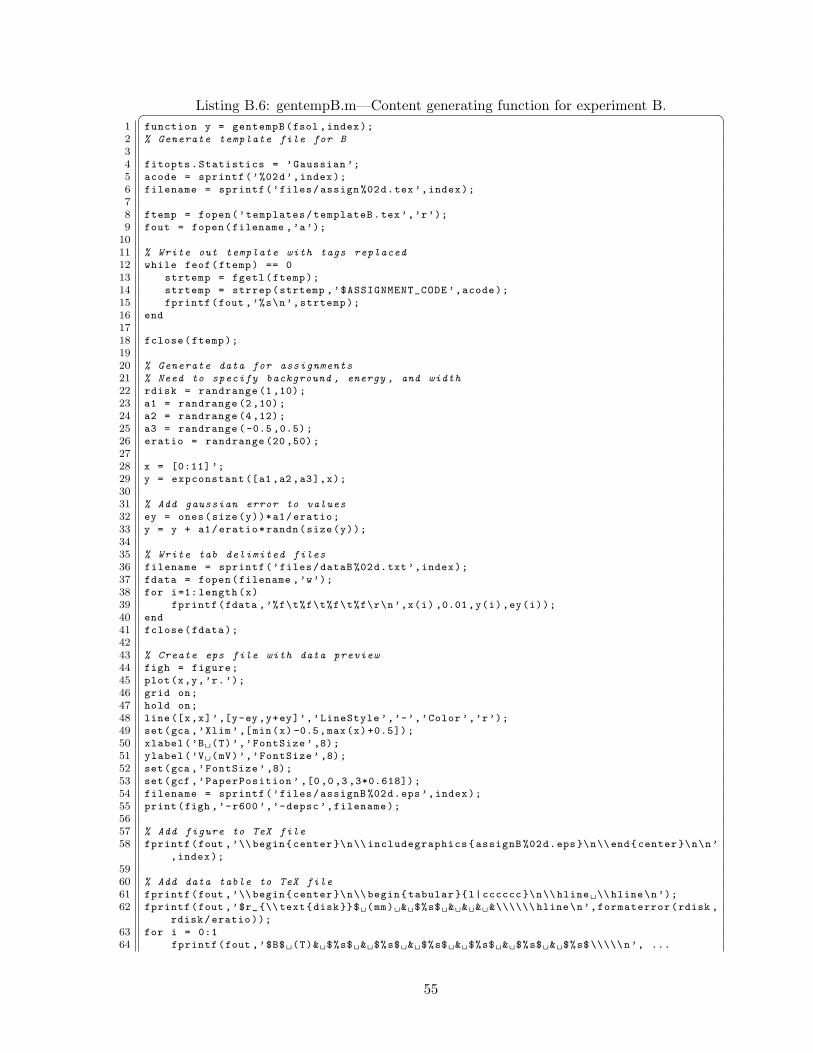
Listing B.6: gentempB.m—Content generating function for experiment B.¨ ¥1 function y = gentempB(fsol ,index);

2 % Generate template file for B

34 fitopts.Statistics = ’Gaussian ’;

5 acode = sprintf(’%02d’,index);

6 filename = sprintf(’files/assign %02d.tex’,index);

78 ftemp = fopen(’templates/templateB.tex’,’r’);

9 fout = fopen(filename ,’a’);

1011 % Write out template with tags replaced

12 while feof(ftemp) == 0

13 strtemp = fgetl(ftemp);

14 strtemp = strrep(strtemp ,’$ASSIGNMENT_CODE ’,acode);

15 fprintf(fout ,’%s\n’,strtemp);

16 end

1718 fclose(ftemp);

1920 % Generate data for assignments

21 % Need to specify background , energy , and width

22 rdisk = randrange (1,10);

23 a1 = randrange (2,10);

24 a2 = randrange (4,12);

25 a3 = randrange ( -0.5 ,0.5);

26 eratio = randrange (20 ,50);

2728 x = [0:11] ’;

29 y = expconstant ([a1,a2,a3],x);

3031 % Add gaussian error to values

32 ey = ones(size(y))*a1/eratio;

33 y = y + a1/eratio*randn(size(y));

3435 % Write tab delimited files

36 filename = sprintf(’files/dataB %02d.txt’,index);

37 fdata = fopen(filename ,’w’);

38 for i=1: length(x)

39 fprintf(fdata ,’%f\t%f\t%f\t%f\r\n’,x(i) ,0.01,y(i),ey(i));

40 end

41 fclose(fdata);

4243 % Create eps file with data preview

44 figh = figure;

45 plot(x,y,’r.’);

46 grid on;

47 hold on;

48 line([x,x]’,[y-ey ,y+ey]’,’LineStyle ’,’-’,’Color’,’r’);

49 set(gca ,’Xlim’,[min(x) -0.5,max(x)+0.5]);

50 xlabel(’BÃ(T)’,’FontSize ’ ,8);

51 ylabel(’VÃ(mV)’,’FontSize ’ ,8);

52 set(gca ,’FontSize ’ ,8);

53 set(gcf ,’PaperPosition ’ ,[0 ,0 ,3 ,3*0.618]);

54 filename = sprintf(’files/assignB %02d.eps’,index);

55 print(figh ,’-r600’,’-depsc’,filename);

5657 % Add figure to TeX file

58 fprintf(fout ,’\\begin{center }\n\\ includegraphics{assignB %02d.eps}\n\\end{center }\n\n’

,index);

5960 % Add data table to TeX file

61 fprintf(fout ,’\\begin{center }\n\\ begin{tabular }{l|cccccc }\n\\ hlineÃ\\hline\n’);

62 fprintf(fout ,’$r_ {\\ text{disk}}$Ã(mm)Ã&Ã$%s$Ã&Ã&Ã&Ã&\\\\\\ hline\n’,formaterror(rdisk ,

rdisk/eratio));

63 for i = 0:1

64 fprintf(fout ,’$B$Ã(T)&Ã$%s$Ã&Ã$%s$Ã&Ã$%s$Ã&Ã$%s$Ã&Ã$%s$Ã&Ã$%s$\\\\\n’, ...

55

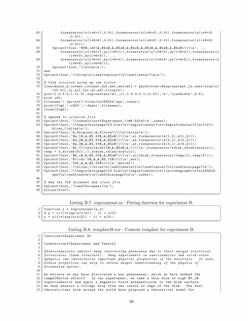
65 formaterror(x(i*6+1) ,0.01),formaterror(x(i*6+2) ,0.01),formaterror(x(i*6+3)

,0.01), ...

66 formaterror(x(i*6+4) ,0.01),formaterror(x(i*6+5) ,0.01),formaterror(x(i*6+6)

,0.01));

67 fprintf(fout ,’$V$Ã(mV)&Ã$%s$Ã&Ã$%s$Ã&Ã$%s$Ã&Ã$%s$Ã&Ã$%s$Ã&Ã$%s$\\\\\n’, ...

68 formaterror(y(i*6+1) ,ey(i*6+1)),formaterror(y(i*6+2) ,ey(i*6+2)),formaterror(y

(i*6+3),ey(i*6+3)), ...

69 formaterror(y(i*6+4) ,ey(i*6+4)),formaterror(y(i*6+5) ,ey(i*6+5)),formaterror(y

(i*6+6),ey(i*6+6)));

70 fprintf(fout ,’\\hline\n’);

71 end

72 fprintf(fout ,’\\hline\n\\end{tabular }\n\\end{center }\n\n’);

7374 % Find solution using my own fitter

75 [residuals ,A,covmat ,corrmat ,dof ,met ,metcdf] = physfitter(@expconstant ,[x,ones(size(x)

)*0.01] ,[y,ey],[a1 ,a2,a3],fitopts);

76 plot ([ -0.5:0.1:11.5] , expconstant(A(:,1) ,[ -0.5:0.1:11.5]) ,’k’,’LineWidth ’ ,0.5);

77 hold off;

78 filename = sprintf(’files/solB %02d.eps’,index);

79 print(figh ,’-r600’,’-depsc’,filename);

80 close(figh);

8182 % Append to solution file

83 fprintf(fsol ,’\\ subsection *{ ExperimentÃ\\#B-%02d}\n’,index);

84 fprintf(fsol ,’\\begin{minipage }{3.5in}\n\\begin{center }\n\\begin{tabular }{lrr}\n\\

hlineÃ\\hline\n’);

85 fprintf(fsol ,’&ÃOriginalÃ&ÃFitted \\\\\n\\ hline\n’);

86 fprintf(fsol ,’$a_1$Ã&Ã$%.3f$Ã&Ã$%s$\\\\\n’,a1,formaterror(A(1,1),A(1,2)));

87 fprintf(fsol ,’$a_2$Ã&Ã$%.3f$Ã&Ã$%s$\\\\\n’,a2,formaterror(A(2,1),A(2,2)));

88 fprintf(fsol ,’$a_3$Ã&Ã$%.3f$Ã&Ã$%s$\\\\\n’,a3,formaterror(A(3,1),A(3,2)));

89 fprintf(fsol ,’$r_ {\\ text{disk}}$Ã&Ã$%s$Ã&Ã\\\\\n’,formaterror(rdisk ,rdisk/eratio));

90 temp = e_divide(A(1,:) ,[rdisk ,rdisk/eratio ]);

91 fprintf(fsol ,’$E_c$Ã&Ã$%.3f$Ã&Ã$%s$\\\\\n’,a1/rdisk ,formaterror(temp (1),temp (2)));

92 fprintf(fsol ,’$\\chi^2$Ã&Ã&Ã$%.1f$\\\\\n’,met);

93 fprintf(fsol ,’CDFÃ&Ã&Ã$%.3f$\\\\\n’,metcdf);

94 fprintf(fsol ,’\\hlineÃ\\hline\n\\end{tabular }\n\\end{center }\n\\end{minipage }\n’);

95 fprintf(fsol ,’\\begin{minipage }{3.5in}\n\\begin{center }\n\\ includegraphics{solB %02d.

eps}\n\\end{center }\n\\end{minipage }\n\n’,index);

9697 % End the TeX document and close file

98 fprintf(fout ,’\\end{document }\n’);

99 fclose(fout);­§ ¦

Listing B.7: expconstant.m—Fitting function for experiment B.¨ ¥1 function y = expconstant(a,x)

2 % y = a(1) *( exp(x/a(2)) - 1) + a(3)

3 y = a(1)*(exp(x/a(2)) - 1) + a(3);­§ ¦

Listing B.8: templateB.tex—Content template for experiment B.¨ ¥1 \section *{ Experiment B}

23 \subsection *{ Experiment and Theory}

45 % Semiconductors exhibit many interesting phenomena due to their unique electrical

6 % structures (band structure). Many experiments in semiconductor and solid -state

7 %physics can characterize important physical properties of the materials . In turn ,

8 %these properties can help to obtain deeper understanding of the physics of

9 %condensed matter.

1011 We believe we may have discovered a new phenomenon , which we have dubbed the

12 \emph{Harlow effect }. In our experiment , we take a thin disk of high $T_c$

13 superconductor and apply a magnetic field perpendicular to the disk surface.

14 We then measure a voltage drop from the centre to edge of the disk. The best

15 theoreticians from around the world have proposed a theoretical model for

56

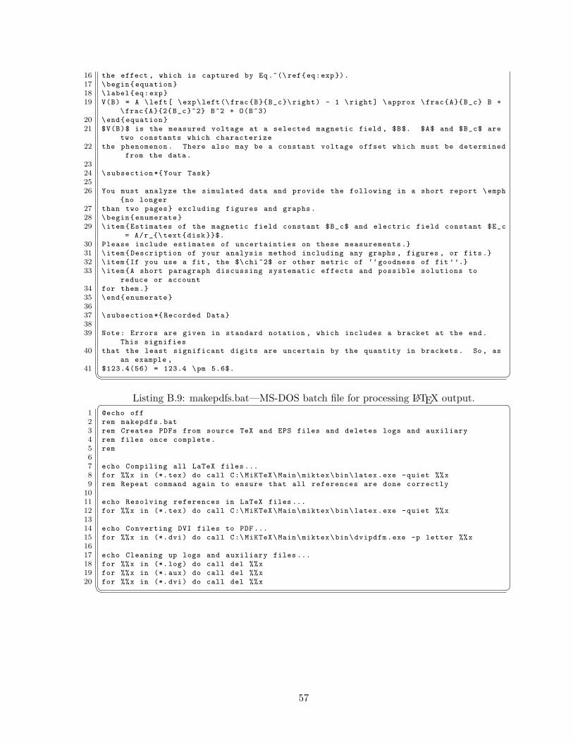
16 the effect , which is captured by Eq.~(\ ref{eq:exp}).

17 \begin{equation}

18 \label{eq:exp}

19 V(B) = A \left[ \exp\left(\frac{B}{B_c}\ right) - 1 \right] \approx \frac{A}{B_c} B +

\frac{A}{2{B_c}^2} B^2 + O(B^3)

20 \end{equation}

21 $V(B)$ is the measured voltage at a selected magnetic field , $B$. $A$ and $B_c$ are

two constants which characterize

22 the phenomenon. There also may be a constant voltage offset which must be determined

from the data.

2324 \subsection *{Your Task}

2526 You must analyze the simulated data and provide the following in a short report \emph

{no longer

27 than two pages} excluding figures and graphs.

28 \begin{enumerate}

29 \item{Estimates of the magnetic field constant $B_c$ and electric field constant $E_c

= A/r_{\ text{disk }}$.

30 Please include estimates of uncertainties on these measurements .}

31 \item{Description of your analysis method including any graphs , figures , or fits.}

32 \item{If you use a fit , the $\chi ^2$ or other metric of ‘‘goodness of fit ’’.}

33 \item{A short paragraph discussing systematic effects and possible solutions to

reduce or account

34 for them.}

35 \end{enumerate}

3637 \subsection *{ Recorded Data}

3839 Note: Errors are given in standard notation , which includes a bracket at the end.

This signifies

40 that the least significant digits are uncertain by the quantity in brackets. So, as

an example ,

41 $123.4(56) = 123.4 \pm 5.6$.­§ ¦

Listing B.9: makepdfs.bat—MS-DOS batch file for processing LATEX output.¨ ¥1 @echo off

2 rem makepdfs.bat

3 rem Creates PDFs from source TeX and EPS files and deletes logs and auxiliary

4 rem files once complete.

5 rem

67 echo Compiling all LaTeX files ...

8 for %%x in (*.tex) do call C:\ MiKTeX\Main\miktex\bin\latex.exe -quiet %%x

9 rem Repeat command again to ensure that all references are done correctly

1011 echo Resolving references in LaTeX files ...

12 for %%x in (*.tex) do call C:\ MiKTeX\Main\miktex\bin\latex.exe -quiet %%x

1314 echo Converting DVI files to PDF...

15 for %%x in (*.dvi) do call C:\ MiKTeX\Main\miktex\bin\dvipdfm.exe -p letter %%x

1617 echo Cleaning up logs and auxiliary files ...

18 for %%x in (*.log) do call del %%x

19 for %%x in (*.aux) do call del %%x

20 for %%x in (*.dvi) do call del %%x­§ ¦

57

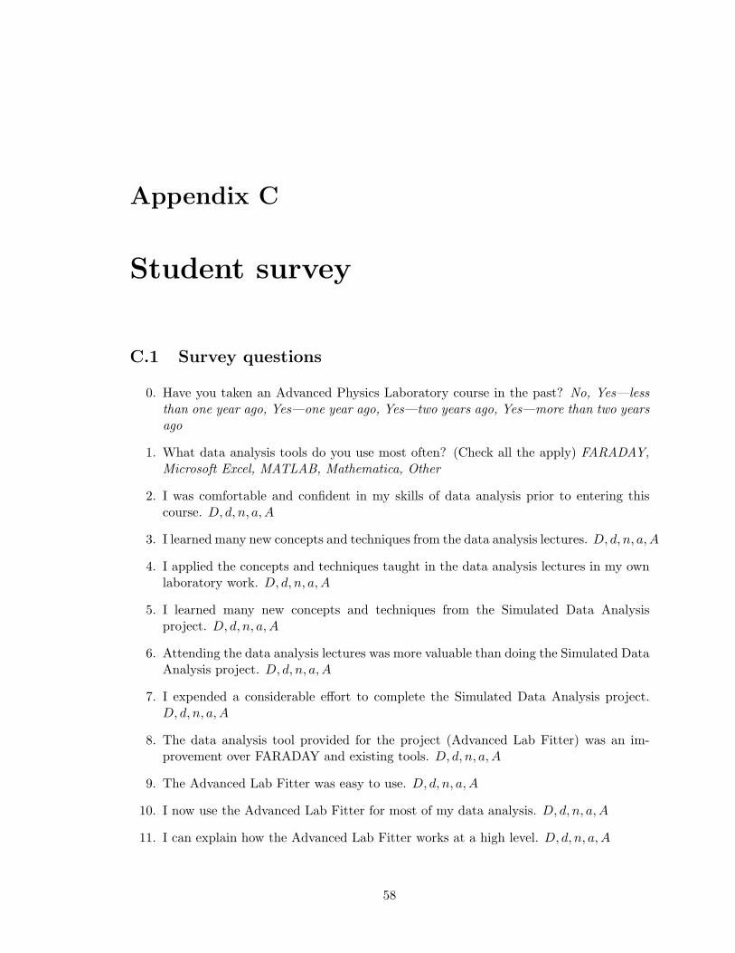
Appendix C

Student survey

C.1 Survey questions

0. Have you taken an Advanced Physics Laboratory course in the past? No, Yes—lessthan one year ago, Yes—one year ago, Yes—two years ago, Yes—more than two yearsago

1. What data analysis tools do you use most often? (Check all the apply) FARADAY,Microsoft Excel, MATLAB, Mathematica, Other

2. I was comfortable and confident in my skills of data analysis prior to entering thiscourse. D, d, n, a, A

3. I learned many new concepts and techniques from the data analysis lectures. D, d, n, a,A

4. I applied the concepts and techniques taught in the data analysis lectures in my ownlaboratory work. D, d, n, a, A

5. I learned many new concepts and techniques from the Simulated Data Analysisproject. D, d, n, a, A

6. Attending the data analysis lectures was more valuable than doing the Simulated DataAnalysis project. D, d, n, a,A

7. I expended a considerable effort to complete the Simulated Data Analysis project.D, d, n, a,A

8. The data analysis tool provided for the project (Advanced Lab Fitter) was an im-provement over FARADAY and existing tools. D, d, n, a, A

9. The Advanced Lab Fitter was easy to use. D, d, n, a,A

10. I now use the Advanced Lab Fitter for most of my data analysis. D, d, n, a, A

11. I can explain how the Advanced Lab Fitter works at a high level. D, d, n, a, A

58

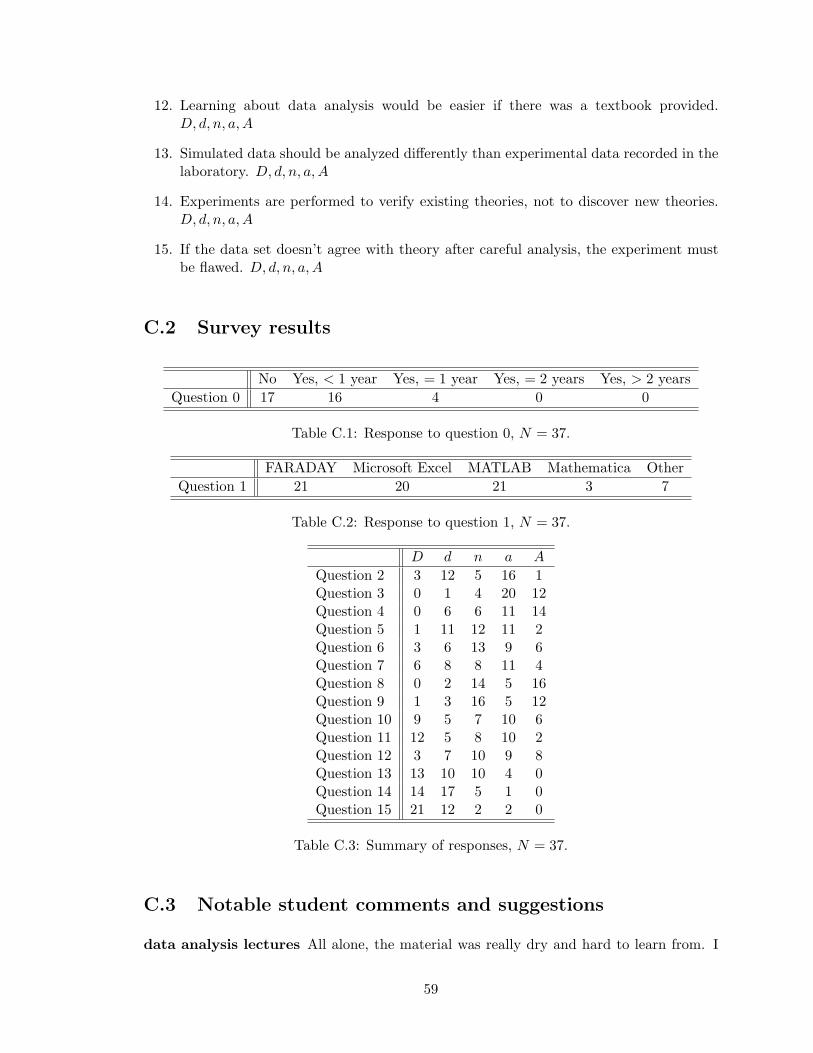
12. Learning about data analysis would be easier if there was a textbook provided.D, d, n, a,A

13. Simulated data should be analyzed differently than experimental data recorded in thelaboratory. D, d, n, a, A

14. Experiments are performed to verify existing theories, not to discover new theories.D, d, n, a,A

15. If the data set doesn’t agree with theory after careful analysis, the experiment mustbe flawed. D, d, n, a,A

C.2 Survey results

No Yes, < 1 year Yes, = 1 year Yes, = 2 years Yes, > 2 yearsQuestion 0 17 16 4 0 0

Table C.1: Response to question 0, N = 37.

FARADAY Microsoft Excel MATLAB Mathematica OtherQuestion 1 21 20 21 3 7

Table C.2: Response to question 1, N = 37.

D d n a A

Question 2 3 12 5 16 1Question 3 0 1 4 20 12Question 4 0 6 6 11 14Question 5 1 11 12 11 2Question 6 3 6 13 9 6Question 7 6 8 8 11 4Question 8 0 2 14 5 16Question 9 1 3 16 5 12Question 10 9 5 7 10 6Question 11 12 5 8 10 2Question 12 3 7 10 9 8Question 13 13 10 10 4 0Question 14 14 17 5 1 0Question 15 21 12 2 2 0

Table C.3: Summary of responses, N = 37.

C.3 Notable student comments and suggestions

data analysis lectures All alone, the material was really dry and hard to learn from. I

59

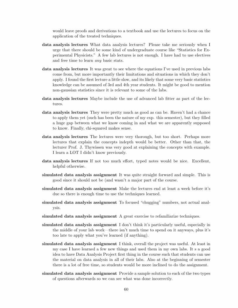
would leave proofs and derivations to a textbook and use the lectures to focus on theapplication of the treated techniques.

data analysis lectures What data analysis lectures? Please take me seriously when Iurge that there should be some kind of undergraduate course like “Statistics for Ex-perimental Physicists.” A few lab lectures is not enough. I have had to use electivesand free time to learn any basic stats.

data analysis lectures It was great to see where the equations I’ve used in previous labscome from, but more importantly their limitations and situations in which they don’tapply. I found the first lecture a little slow, and its likely that some very basic statisticsknowledge can be assumed of 3rd and 4th year students. It might be good to mentionnon-gaussian statistics since it is relevant to some of the labs.

data analysis lectures Maybe include the use of advanced lab fitter as part of the lec-tures.

data analysis lectures They were pretty much as good as can be. Haven’t had a chanceto apply them yet (such has been the nature of my exp. this semester), but they filleda huge gap between what we know coming in and what we are apparently supposedto know. Finally, chi-squared makes sense.

data analysis lectures The lectures were very thorough, but too short. Perhaps morelectures that explain the concepts indepth would be better. Other than that, thelecturer Prof. J. Thywissen was very good at explaining the concepts with example.I learn a LOT I didn’t know previously.

data analysis lectures If not too much effort, typed notes would be nice. Excellent,helpful otherwise.

simulated data analysis assignment It was quite straight forward and simple. This isgood since it should not be (and wasn’t a major part of the course.

simulated data analysis assignment Make the lectures end at least a week before it’sdue so there is enough time to use the techniques learned.

simulated data analysis assignment To focused “chugging” numbers, not actual anal-ysis.

simulated data analysis assignment A great exercise to refamiliarize techniques.

simulated data analysis assignment I don’t think it’s particularly useful, especially inthe middle of your lab work—there isn’t much time to spend on it anyways, plus it’stoo late to apply what you’ve learned (if anything).

simulated data analysis assignment I think, overall the project was useful. At least inmy case I have learned a few new things and used them in my own labs. It s a goodidea to have Data Analysis Project first thing in the course such that students can usethe material on data analysis in all of their labs. Also at the beginning of semesterthere is a lot of free time, so students would be more inclined to do the assignment.

simulated data analysis assignment Provide a sample solution to each of the two typesof questions afterwards so we can see what was done incorrectly.

60

simulated data analysis assignment I think it may have been too easy—not many fac-tors to consider. Our labs require much more complex analysis.

simulated data analysis assignment I did not like it. Deciphering the theory tookawhile, and the workload for this course is too high as it is. The time could bebetter spent I think.

advanced lab fitter This touches on the data analysis project as well. Make the assign-ment in two parts: a) A more complicated analysis with necessary fitting equationsprovided. b) Simpler raw data that requires the student to decide how to fit it. Thiswould be much closer to lab reality. Though hard to find the right way to put it ina project. Is it possible to expand it (the Fitter) to 3-dimensions? This would allowfor some interesting modelling.

advanced lab fitter Add more post fitting analysis tools like in the MATLAB curve fittingtoolbox. This includes extrapolation and integration tools. Also, make it easier toenter data sets, like a setting for a constant error instead of a vector.

advanced lab fitter The fitter is the best program I’ve used, ever!! So easy to use. Myonly concern is that the fit equations are predefined. Maybe an option that allows usto input our own equations would be nice → kind of like the program Kaleida Graph.Other than that, it is amazing!! I use it for a lot of my other courses and labs now.

advanced lab fitter I downloaded the fitter and got MATLAB. However, did not endup using the fitter for 2 reasons. 1) No clear instruction for starting up. 2) Quiteintimidating to the new user. Maybe adding a step by step fit procedure to the manualshowing how a hit is done would be useful.

61