The determination of ecological status in shallow lakes ...pcpelagic/s/Moss et al 2003(2).pdf · ABSTRACT 1. The European Water Framework Directive requires the determination of ecological

Copyright # 2003 John Wiley & Sons, Ltd. Received 28 June 2002Accepted 29 November 2002

AQUATIC CONSERVATION: MARINE AND FRESHWATER ECOSYSTEMS

Aquatic Conserv: Mar. Freshw. Ecosyst. 13: 507–549 (2003)

Published online in Wiley InterScience(www.interscience.wiley.com). DOI: 10.1002/aqc.592

The determination of ecological status in shallow lakes } atested system (ECOFRAME ) for implementation of the

European Water Framework Directive

BRIAN MOSSa*, DEBORAH STEPHENa, CRISTINA ALVAREZb, ELOY BECARESb,WOUTER VAN DE BUNDc, S.E. COLLINGSa, ELLEN VAN DONKc, ELVIRA DE EYTOd,T *OONNU FELDMANNe,f, CAMINO FERN !AANDEZ-AL !AAEZb, MARGARITA FERN !AANDEZ-

AL !AAEZb, ROB J.M. FRANKENg, FRANCISCO GARC!IIA-CRIADOb, ELISABETH M. GROSSh,MIKAEL GYLLSTR .OOMi, LARS-ANDERS HANSSONi, KENNETH IRVINEd, AIN J .AARVALTe,JENS-PEDER JENSENj, ERIK JEPPESENj,k, TIMO KAIRESALOl, RYSZARD KORNIJ !OOWm,TEET KRAUSEe,f, HELEN K .UUNNAPe, ALO LAASe, EVI LILLe, BOGDAN LORENSn, HELENLUUPe, MARIA ROSA MIRACLEo, PEETER N *OOGESe,f, TIINA N *OOGESe,f, MIRVA NYK .AANENl,

INGMAR OTTe, WOJCIECH PECZULAp, EDWIN T.H.M. PEETERSg, GEOFF PHILLIPSq,SUSANNA ROMOo, VICTORIA RUSSELLa, JAANA SALUJ *OOEe,f, MARTEN SCHEFFERg,

KLAUS SIEWERTSENc, HALINA SMALr, CLAUDIA TESCHh, HENN TIMMe, LEA TUVIKENEe,ILMAR TONNOe,f, TAAVI VIRROf, EDUARDO VICENTEo and DAVID WILSONa

aSchool of Biological Sciences, Derby Building, University of Liverpool, Liverpool L69 3GS, UK; bInstituto de Medio

anbiente, La Serna 56, 24007, Leon, Spain; cNational Institute of Ecology, Centre for Limnology, 1299, 3600 BG,

Maarssen, 3631A Nieuwersluis, The Netherlands; dDepartment of Zoology, University of Dublin, Trinity College, Dublin

2, Ireland; eEstonian Agricultural University, Institute of Zoology and Botany, V *oortsjarv Limnological Station, 61101

Rannu, Tartu County, Estonia; fUniversity of Tartu, Institute of Zoology and Hydrobiology, 46 Vanemuise Str., 51014

Tartu, Estonia; gAquatic Ecology and Water Quality Management Group, Wageningen University, PO Box 8080 6700

DD Wageningen, The Netherlands; hFachbereich Biologie, Limnologisches Institut, Postfach M 659, University of

Konstanz } 78547, Konstanz, Germany; iDept of Limnology, University of Lund, Lund, Sweden; jDepartment of

Freshwater Ecology, National Environmental Research Institute, Vejlsøvej 25, Silkeborg, Denmark; kDepartment of

Botanical Ecology, University of Aarhus, Norlandsvej 63, 8230 Risskov, Denmark; lDepartment of Ecological &

Environmental Sciences, University of Helsinki, Niemenkatu 79, FIN-15140 Lahti, Finland; mDepartment of

Hydrobiology and Ichthyobiology, University of Agriculture in Lublin, Lublin 20-950, Poland; nDepartment of Ecology,

Maria Curie Sklodowska University, Lublin, Poland; oArea de Ecologıa, Faculdad Biologıa et Investigacion, Campus

Burjasot, 46100 Burjasot, Valencia, Spain; pDepartment of Botany and Hydrobiology, Catholic University of Lublin,

Lublin, Poland; qEnvironment Agency, UK; rInstitute of Soil Science and Environment Management, University of

Agriculture in Lublin, Lublin, Poland

*Correspondence to: Prof. Brian Moss, School of Biological Sciences, Derby Building, University of Liverpool, Liverpool L69 3GS,UK. E-mail: [email protected]

ABSTRACT

1. The European Water Framework Directive requires the determination of ecological status inEuropean fresh and saline waters. This is to be through the establishment of a typology of surfacewater bodies, the determination of reference (high status) conditions in each element (ecotype) of thetypology and of lower grades of status (good, moderate, poor and bad) for each ecotype. It thenrequires classification of the status of the water bodies and their restoration to at least ‘good status’in a specified period.2. Though there are many methods for assessing water quality, none has the scope of that defined

in the Directive. The provisions of the Directive require a wide range of variables to be measured andgive only general guidance as to how systems of classification should be established. This raises issuesof comparability across States and of the costs of making the determinations.3. Using expert workshops and subsequent field testing, a practicable pan-European typology and

classification system has been developed for shallow lakes, which can easily be extended to all lakes.It is parsimonious in its choice of determinands, but based on current limnological understandingand therefore as cost-effective as possible.4. A core typology is described, which can be expanded easily in particular States to meet local

conditions. The core includes 48 ecotypes across the entire European climate gradient andincorporates climate, lake area, geology of the catchment and conductivity.5. The classification system is founded on a liberal interpretation of Annexes in the Directive and

uses variables that are inexpensive to measure and ecologically relevant. The need for taxonomicexpertise is minimized.6. The scheme has been through eight iterations, two of which were tested in the field on tranches

of 66 lakes. The final version, Version 8, is offered for operational testing and further refinement bystatutory authorities.Copyright # 2003 John Wiley & Sons, Ltd.

KEY WORDS: lakes; Water Framework Directive; typology; ecotypes; ecological status; quality

INTRODUCTION

The European Water Framework Directive (Directive 2000/60/EC of the European Parliament and of TheCouncil of 23 October 2000 establishing a framework for Community action in the field of water policy) ispotentially the most significant piece of legislation ever to be enacted in the interests of conservation offresh and saline ecosystems (Pollard and Huxham, 1998). It seeks to replace legislation that hasconcentrated on emission standards for water quality, with little reference to ultimate ecologicalconsequences. Its approach is to work backwards from ultimate targets for ecological quality to whateverlegal and practical measures are necessary to achieve these targets. It also uses biological measures to agreater extent than previously, when water quality based largely on chemical determinands has beenemphasized. The distinction between water quality and ecological quality is very considerable and systemscurrently used to establish the former are only a small part of those needed for the latter.

The Directive requires catchments to be managed in a holistic way, reflecting the connectedness thatexists between the landscape and its uses, and the nature of the water that runs off it into flowing andstanding waters and groundwaters and eventually to estuaries and the sea. The ultimate effectiveness of thismeasure will be reflected in the degree to which aquatic habitats are restored, over the next 15 years andbeyond, to ‘good’ ecological status. ‘Good ecological status’ is the ultimate target and ‘status’ as used in theDirective is synonymous with ‘quality’. The Directive requires, first of all, a typology among flowing,standing, transitional (estuarine) and coastal waters. In each of these general groups, types, (‘ecotypes’ isthe term used in the Directive), must be defined and reference conditions (or ‘high status’) for each typedetermined. Then, for each ecotype, a classification system must be established in which deviations fromthis high quality status must be determined.

These classes are called ‘good’, ‘moderate’, ‘poor’ and ‘bad’ and must be determined by the use ofbiological and chemical characteristics with hydromorphology appropriate to achievement of these

B. MOSS ET AL.508

Copyright # 2003 John Wiley & Sons, Ltd. Aquatic Conserv: Mar. Freshw. Ecosyst. 13: 507–549 (2003)

chemical and biological characteristics. The Directive lists the characteristics that must be assessed but givesonly general guidance as to the nature of these levels of quality. High status is defined in the Directive suchthat there are ‘ no, or only very minor anthropogenic alterations’ to the chemistry, physics, morphologyand hydrology of the water body and that values of biological quality elements ‘reflect those normallyassociated with that type under undisturbed conditions, and show no, or only very minor, evidence ofdistortion’. High status is thus very close to pristine conditions.

European Directives indicate the spirit of legislation that must be put into operation through nationallegislation by Member States. Their effect may be weakened by the use of derogations built into the Directivesin the process of their being agreed by all States in the European Parliament. Cost of remedial action and ofmonitoring is also an issue. Inevitably, faced with many demands on their budgets and the balance of lobbyingby vested interests of all kinds, governments are faced with much compromise and the degree to which theremight be delays in the enactment of Directives becomes a highly political issue. Conservation is likely to be amajor loser as a result of these influences. Uncertainties about how to fulfil the intentions of Directives mayalso delay implementation. The Water Framework Directive is especially vulnerable to this. It is complexlegislation attempting to measure what is inherently very difficult, for degrees of ecological quality are notabsolute but matters of judgement. This paper contributes a tool to help overcome at least this problem.

There are at least two approaches to establishing a system for measuring ecological status. The first is todiscuss it extensively among the ‘competent authorities’, the statutory agencies charged with implementingthe Directive, in the hope that some wide consensus may emerge, and then attempt to create commonsystems for measuring it. At present numerous meetings are being held throughout Europe in the hope ofachieving this. Every European country has some scheme for reaching some of the objectives of theDirective and each is attempting to incorporate its existing schemes into new systems to fulfil the greaterends of the Directive. This is understandable, given the accumulated data sets on water quality againstwhich future change must be assessed. Likewise, bodies (10 working groups of the Strategic Co-ordinationGroup) have been set up by the European Commission to find common approaches.

However, no existing scheme is entirely satisfactory for none has been set up to measure ecological statusas opposed to water quality. For rivers there are some schemes which take into account more than waterchemistry (for example RIVPACS (Wright et al., 2000); SERCON (Boon, 2000) and River Habitat Survey(Raven et al., 1997)) but there are no equivalents for lakes. General approaches to monitoring water qualityare often vested in the ultimate solution of the nineteenth and early twentieth century crisis of gross organicpollution by raw sewage (Hynes, 1970; Kristensen and Hanson, 1994). They have little to say about thecurrent problems of eutrophication, acidification, introduced species, engineering damage, water abstractionand pollution by metabolically powerful trace organic substances, all of which are central to the restorationof good ecological status. New philosophies, created by modern problems, demand new brooms.

It is perhaps then necessary to learn from previous schemes but go back to ecological principles andcurrent scientific understanding and create a fresh, simple scheme that will be immediately workable. Oneway to do this is to bring together groups of expert ecologists, with practical knowledge of the systems, toagree on schemes that make ecological sense and then to test them to discover and solve practicaloperational problems in an iterative way, until a workable solution is reached. This paper concerns such anapproach and records the process of developing a usable scheme, in the first instance for shallow lakes, butpotentially extendable to all lakes.

THE DIRECTIVE AND LAKES

Establishing a typology

Standing waters are one of the four main surface water categories to be dealt with under the Directive. Thefirst problem is to establish a typology, the second a system of measuring ecological status. Annex II of the

THE DETERMINATION OF ECOLOGICAL STATUS IN SHALLOW LAKES 509


Directive suggests two approaches to a typology of lakes. System A is given in detail and embraces 25biogeographical regions, three categories of altitude, four for area, three for depth and three for immediategeology (organic, siliceous, calcareous). This gives a total of 2700 potential ecotypes, although not allaltitudinal, depth, areal and geological combinations might occur in each biogeographical region. Arealistic assessment might give more than a thousand ecotypes however. Alternatively, System B allowsStates to propose a different system, as long as it gives at least as good resolution as System A and suggestssome other variables that might be used to establish the typology.

Two issues are important in the establishment of a typology. First, it should not be so complicated thatconditions of high ecological status cannot easily be defined for every one of the ecotypes. Second, and mostimportantly, it should use only characteristics that are geographical and do not overlap with the variablesused in measuring ecological status, otherwise a very confused system will result. For lakes, System A asproposed is undoubtedly too complex. It uses only geographical features but it omits some characteristics,such as climate and conductivity, that might be more valuable in establishing a limnologically meaningfulscheme than the ones it proposes.

System B, as exemplified in Annex II, poses a very great danger in that it suggests nutrients might be usedas a variable in establishing the typology. Clearly, changing nutrient loading is one of the key characteristicsaffecting ecological status and it would be most inadvisable to use it as a component of a typology. SystemB, however, offers the flexibility of producing a simpler, practicable, typology and, importantly, has theoption of including small lakes, many of which are of considerable amenity and conservation importance.System A excludes these by using a minimum lake area of 50 ha.

CLASSIFICATION OF ECOLOGICAL STATUS

The Directive requires the establishment of reference conditions (high ecological status) for each of theecotypes in the typology. These reference conditions can be determined from existing sites, from models,from palaeolimnological reconstructions and from expert judgement or from some combination of these.This is the closest the Directive comes to establishing general criteria that are close to objective because itdefines high ecological status as a state insignificantly influenced by human activity. Thereafter theestablishment of degrees of quality can only be through expert judgement, there being no absolutemeanings of good, moderate, poor and bad. One of these terms is itself used in its own definition in AnnexV of the Directive, thus offending a basic principle of lexicography.

Establishment of the reference conditions is not easy for there are few, if any, such sites available inEurope for all but polar and montane areas and even there the incidence of climate warming, increasedultra violet exposure (Sommaruga-W .oograth et al., 1997) and air-borne pollutants make it unlikely that trulyhigh status sites exist. The use of multivariate data analysis on large data sets from many lakes, despitemuch investment, and faith in it as an objective way of determining groupings of sites, cannot be used fordetermining reference conditions. Such methods do give groupings, albeit often not very tightly defined, butbecause the lakes from which the data are derived have been subject to varied degrees of change from avariety of sources, the groupings are only artefacts of the individual states of impact at the time the datawere collected and can have no absolute value.

Palaeolimnology (Vallentyne, 1969) has developed considerably during the last decade, not least bydevelopment of training sets and transfer functions allowing reconstruction of changes in variables such aspH, concentration of total phosphorus, salinity, abundance of planktivorous fish, coverage of submergedmacrophytes and relative contribution of various algae (Bennion et al., 1995, 1996; Jeppesen et al.,1996,2001a; Sayer, 2001). Reconstruction of some chemical variables, such as pH (ter Braak and Van Dam,1989), which change on logarithmic scales, has been very reliable but for other chemical variables, whichchange arithmetically, the reconstructions are often subject to variabilities that cover more than one order

B. MOSS ET AL.510


of magnitude (Bennion et al, 1995, 1996; Sayer, 2001) and this is too great for precise reconstruction ofreference conditions. The major changes in nutrient status that have occurred in British rural catchmentssince before World War II, for example, have embraced only a doubling, on average, in nutrient loadings(Johnes et al., 1996). However, there is great potential for modern palaeolimnogical reconstructions inhelping identify the general characteristics of reference conditions. The techniques are improving rapidly sothat more precise reconstructions will eventually be possible especially by using arrays of differentorganisms in sediments (multi-proxy approaches), calibrated from similar arrays under current conditions.

Determination of reference states is therefore currently best approached through a combination of expertjudgement based on experience, available data, hindcasting using export coefficient models (Johnes, 1996)and palaeolimnology. The process is likely to depend a great deal on the accumulation of experience andintegration from all these lines of evidence rather than on a statistically rigorous procedure. It thereforeneeds the consensus of groups of well informed ecologists.

In reconstructing lesser ecological quality states, there are again at least two approaches. One is to definevalues for chemical and biological variables that are supposed to be fixed norms for each state and tocompile the whole from the sum of these. This is the approach likely to be adopted naturally byorganizations which have managed water quality in the past, largely from the viewpoint of chemicalcompliance.

There is, however, no single set of conditions that represents high ecological status in a given place.Ecosystems are complex and their characteristics mutually vary within large ranges, determined not only byexternal conditions such as weather and catchment characteristics but by internal processes. The uptake ofsubstances by primary producers, their release by grazers and decomposers and the influence of predationon the grazers and on the predators by their own predators lead to an infinite number of normalcombinations of values of thousands of measurable variables. Every ecosystem exists, even in the absence ofhuman impacts, in many alternative states (May, 1977; Scheffer et al., 1993), sometimes transient,sometimes quasi-stable, none of which necessarily represents a superior quality to any of the others.Ecosystems cannot be prescribed by single formulae.

The second approach is to create a picture of the general characteristics of what an ecosystem would havein its high quality state. Overall structure is the most important common feature, the crucial stage on whichecological action takes place. The procedure is then to work back to prescribe the ranges of values ofdeterminands that could correspond with this scenario. This approach acknowledges that any particularvariable will be very likely to give hugely variant values when a single or only a few samples are taken andthus must use a range of variables as a set of insurance policies in arriving at a sensible assessment. Thisapproach is inherently built into the Water Framework Directive by its stipulation of a range ofcharacteristics that must be measured.

Because the Directive places a great deal of emphasis on the maintenance or restoration of ‘good’ecological status, more importance attaches to defining this than to lesser states. Guidance given in AnnexV (Table 1.2) for good status is very stringent: ‘The values of the biological quality elements for the surfacewater body type show low levels of disturbance resulting from human activity, but deviate only slightly fromthose normally associated with the surface water body type under undisturbed conditions’. On this definition itis doubtful that very many current water bodies of good status still exist in Europe. A pragmatic approachwill have to give considerable breadth to the definition of ‘slightly’.

One solution, which accepts that much of Europe will remain generally heavily agricultural andfrequently highly populated, is to use, for good status, the baseline state determined for comparison ofcurrent states in lakes by Moss et al. (1997) and subsequently developed. This proposed that a desirablebaseline state would be one in which the land use was genuinely sustainable } that it would reflect naturalclimatic, topographic and geological conditions and not be a usage maintainable only by import of largequantities of energy and materials, that there would be no net accumulation of alien substances nor of highquantities of native substances, and that the currently most efficient technology be used to treat urban and



industrial wastes also to meet these conditions. In practice, most of these conditions were met by the natureof land use prevalent in the early twentieth century, prior to the agricultural intensification that followedWorld War II.

METHOD OF APPROACH

These principles have been put into practice in developing a typology and a quality classification system forshallow lakes. These lakes were chosen because they are among the most complex ecologically of standingwaters and the problems they pose for typology and classification could allow easy extension of the schemeto all lakes. The scheme was tested by sampling more than 100 lakes in 2 years to discover the practicaldifficulties, recording the time taken for sampling and processing and comparing the results with moreinformal judgements. All of the 12 laboratories involved have considerable experience in research on theecology of shallow lakes and some have been very influential in revising an ecological view of these lakes inthe past 30 years (Irvine et al., 1989; Jeppesen et al., 1990, 1998, 2001b; Scheffer et al., 1993; Moss et al.,1994, 1996, 1998; Van Donk and Gulati, 1995; Hansson et al., 1998; Scheffer, 1998).

The approach was to integrate experience, very large data sets accumulated by the NationalEnvironmental Research Institute, Denmark (Jeppesen et al., 1997, 2001b) and expert judgement, in aseries of residential workshops, to create the typology with the express aim of making it both ecologically

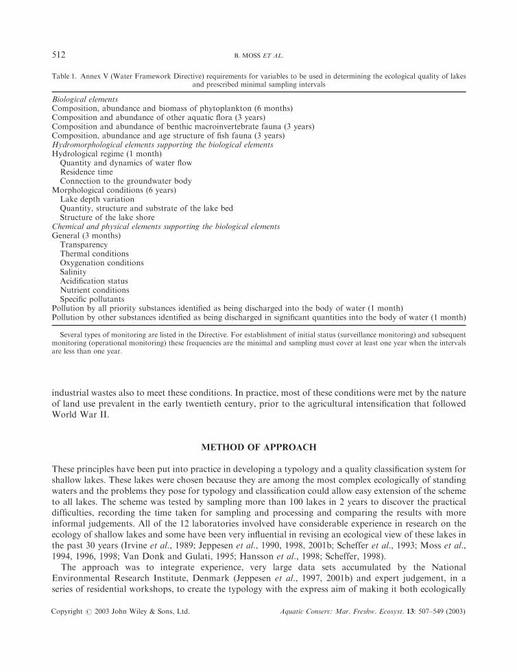
Table 1. Annex V (Water Framework Directive) requirements for variables to be used in determining the ecological quality of lakesand prescribed minimal sampling intervals

Biological elementsComposition, abundance and biomass of phytoplankton (6 months)Composition and abundance of other aquatic flora (3 years)Composition and abundance of benthic macroinvertebrate fauna (3 years)Composition, abundance and age structure of fish fauna (3 years)Hydromorphological elements supporting the biological elementsHydrological regime (1 month)Quantity and dynamics of water flowResidence timeConnection to the groundwater body

Morphological conditions (6 years)Lake depth variationQuantity, structure and substrate of the lake bedStructure of the lake shore

Chemical and physical elements supporting the biological elementsGeneral (3 months)TransparencyThermal conditionsOxygenation conditionsSalinityAcidification statusNutrient conditionsSpecific pollutants

Pollution by all priority substances identified as being discharged into the body of water (1 month)Pollution by other substances identified as being discharged in significant quantities into the body of water (1 month)

Several types of monitoring are listed in the Directive. For establishment of initial status (surveillance monitoring) and subsequentmonitoring (operational monitoring) these frequencies are the minimal and sampling must cover at least one year when the intervalsare less than one year.

B. MOSS ET AL.512


relevant and simple enough to be manageable, whilst also being applicable to all of Europe. It was createdas a core scheme whose categories can be sub-divided to meet particular local conditions. However, thisprocess was resisted in development because every such sub-division doubles the number of ecotypes in ageometric series. In the same workshops a series of scenarios was constructed of what conditions wereenvisaged as characterizing high quality for the 48 shallow-lake ecotypes of the final scheme.

Concurrently the variables which might best be used to characterize these scenarios were decided, withminimal redundancy but maximal probability of measuring features that contributed to the concept ofecological quality. The key feature in choosing variables had to be ecological significance. This may meanthat some variables chosen are ones with high variability rather than high predictability. It is better toemphasize accuracy (in the statistical sense that variables assess what they are intended to assess) over usingvariables which can be rigorously predicted (high precision, often chemical determinands) but which areecologically relatively unimportant. Indeed a variable that is relatively invariable is likely to be leastimportant ecologically.

In 2000, following discussions in which over 100 variables were considered, more than 50 were measuredon a series of 66 lakes to discover whether they had the anticipated predictive value and also to discoverhow long each measurement took. Every characteristic required by Annex V of the Directive was covered,sometimes directly, sometimes tangentially. The results were then examined and the range of variablestrimmed down considerably. As many as possible were discarded on considerations of redundancy, cost orlack of sensitivity and the scheme was modified accordingly. In 2001 the evolving scheme was re-tested on aset of 66 lakes and again the results were reviewed to produce the final proposal, known as ECOFRAMEVersion 8. It is suggested that this be used as a starting point for examination under operational, as opposedto research, conditions.

There is no absolute way of determining the validity of any scheme proposing to measure degrees ofecological status below that of high ecological status. Assessments can only be compared amongindependent experts and not against any absolute standard, except in a qualitative way that comparesconditions with those established for reference conditions. No single variable will be reliable in predictingecological status because of the inherent variability of all biological variables. The scheme thus focuses onbiological structure rather than on details of taxonomy of organisms, which also reduces the need forexpert knowledge among users. Assessment must be on a group of variables because of this variability.Techniques developed for assessing water quality, dependent on the statistical variation in only a singlevariable, and therefore a rigorous calculation of probability of the measurement representing trueconditions, are unlikely to be appropriate. How best to make assessments from the data collected is thusalso considered.

DESCRIPTION OF THE ECOFRAME SCHEME

Typology

ECOFRAME typology is in accord with system B which uses only geographical characteristics and appliesto shallow lakes (mean depth below 3m). At high status their productivity would be dominated bycommunities associated with the bottom, either of algae or of macrophytes and associated periphyton,rather than by phytoplankton. Extension of the scheme to all lakes is discussed later. The typology(Appendices 1,2) is applicable throughout Europe and is based on four climate categories (cold, cool,temperate and warm), defined by the period of annual ice cover (greater or less than two months) and themean air temperature of the warmest month. These subsume considerations of latitude, longitude andaltitude, listed in the Directive, into geographical components that can be more readily used to designateecotypes, and cover the region from the Arctic to the Mediterranean.



It then uses two lake area categories, with a threshold of 10 000 ha (100 km2). This separates very largelakes, with major wind effects, from smaller lakes. There was no evidence that the ecological characteristicsof shallow lakes differ fundamentally among lake areas below 10 000 ha down to areas of a few hectares.There are, however, significant differences (owing much to stochastic factors such as chance of colonizationand risk of drying out) in very small lakes (ponds) smaller than 1–3 ha. These are not necessarily included inthe provisions of the Directive. They are excluded from System A but System B offers no minimalrecommendation for area and many lakes of considerable conservation importance are much smaller thanthe 50 ha minimum for System A.

So far this gives eight basic categories of either large or small cold, cool, temperate or warm lakes. Afurther distinction is then made according to the catchment, into peat (organic soil)-based catchments, withmore than 50% of the area covered by peat deposits, and rock-based catchments, with more than 50% oftheir area floored by rock or mineral-based soils. Peaty catchments give brown waters with distinctiveecological features. Within these categories, three classes of conductivity are used. These reflect watersupplied from acid peat or poorly weathered rocks (5100 mS cm�2), from base-rich peat or soils, often fromunderlying calcareous rocks (101-800 mS cm�2) and waters with some saline influence, either from naturalpercolation of marine-derived groundwaters or from high evaporation or even endorheicity (> 800 mS cm�2).

The core typology has 48 ecotypes (4 climate� 2 area� 2 catchment substratum� 3 conductivity).Competent authorities (those responsible for administering the provisions of the Directive) in specific areasmight wish to build on it by sub-dividing the existing categories. Those in boreal regions, for example, maywish to sub-divide the peat-based catchments to reflect different areas of peat coverage and the consequenteffects on the concentrations of brown substances in the water. Mediterranean countries may wish to sub-divide the >800 mS cm�1 conductivity category to reflect the variety of endorheic basins which they have.Many countries may wish to use more area categories, including one for very small lakes, because theseoften have very significant nature conservation significance. The scheme is open-ended and provided thatsub-divisions of the core categories stipulated here are used, should remain robust and comparable acrossmember states.

Ecological state classification } scenarios of quality

The catchments of lakes in Europe would, under pristine conditions, be dominated by tundra in the polarregions, boreal forest in the far north, broad-leaved forest centrally and to the west, shrubby vegetation inthe south and grasslands towards the south-east and east. These landscapes would be unmanaged for theproduction of timber or for services such as grazing. Almost nowhere will this situation persist, though thetundra and boreal regions still bear large tracts of only lightly managed vegetation, with lakes that couldstill be considered of high status under the definitions of the Directive.

The productivity of shallow lakes is dominated under pristine conditions by bottom vegetation.Sometimes, in the short growth season of the polar regions, this comprises algal communities with only fewmacrophytes, largely isoetids or charophytes depending on local conditions. Elsewhere productivity isdominated by macrophytes with associated periphytic algae. Key to high or good ecological status,therefore, is that the lake must still be dominated by stands of appropriate bottom-living primaryproducers.

The nature of the community can be changed by impacts such as acidification, which will lead to adominance of Sphagnum and certain very acid-tolerant species such as Juncus bulbosus, or eutrophication.The latter will lead to greater growths of large competitive macrophytes, as opposed to the shortercharophyte or isoetid species (Blindow, 1992; Moss, 1999) that can persist if they are not forced to competewith increasing crops of periphyton or phytoplankton. A suite of mechanisms, including nitrogencompetition, allelopathy and provision of refuges for animals that graze periphyton and phytoplanktoncombines to preserve the plant communities (Moss, 1999). The concept of good ecological status is thus

B. MOSS ET AL.514


that there should also be persistence of plant communities of sufficient diversity that a single species of themain growth forms } floating leaved and totally submerged } does not predominate.

As impacts increase, only the more tolerant species persist, often restricted to a very few floating-leavedspecies of nymphaeids or lemnids or of Sphagnum. This is considered to mark conditions of moderateecological status. Major switches then occur as impacts increase. Under acid conditions the water maybecome extremely clear as mobilized aluminium flocculates particles and precipitates phosphate butSphagnum will persist. Poor status in acidified lakes will be marked by complete loss of fish and furtherreduced pH. Under eutrophicated conditions, the mechanisms that stabilise the macrophyte communitieswill often fail and there will be a switch to phytoplankton dominance. This will mark the onset of poorcondition in such lakes. Finally, bad conditions will be reflected in either an even greater reduction in pH inacidified lakes or a dominance by only one prominent species or bloom-forming species of phytoplankterfor long periods in summer in eutrophicated ones.

Other impacts are likely, of course. These include development of shorelines for housing or marinas,introduction of exotic species, stocking for angling, toxic pollution, alteration of water levels, recreationaldamage, and many others. These have to be incorporated but many will be lake-specific rather than generic.For generic variables it is possible to stipulate absolute ranges to be expected but for other impactsassessment can best be made on the basis of relative degree of impact.

Ecological status classification } variables used

The Directive gives general guidance on the determination of ecological status. This has been translatedinto specific requirements for each ecotype, based on a minimum number of variables. Ultimately 28 wereused (Appendices 1,2), some of which can be determined by a single visit to the lake.

The scheme was devised to reflect the sampling frequencies stipulated in the Directive. These are ingeneral relatively low compared with the sampling carried out for ecological research purposes and this hasmeant that the scheme depends much less on the incidence of particular taxonomic categories than might beused with very frequent sampling. A sampling of phytoplankton every 6 months, for example, is unable togive data reliable enough to characterize a lake on the basis of representation of specific algal groups suchas the cyanophytes, diatoms and green algae. To do this reliably, sampling every week or two weeks wouldbe necessary and this would be extremely expensive. Reynolds (2002) even suggests that predictability ispossible only at a range of 2 days or fewer.

Specific changes in zooplankton are equally frequent (Makarewicz and Likens, 1975). Financial and timeresources will inevitably be limited for operation of the Directive. This will mean that rather few lakes canbe considered if sampling is intensive, more if it is extensive. The spirit of the Directive in terms of riverbasin management is towards extensiveness and protection of the entire landscape rather thanconcentration only on a few sites of high conservation importance.

In testing the penultimate Version 7 of the scheme, a suite of variables was used that was modified inproducing Version 8, on the basis of the results of testing. The general rationale for the variables used isexplained below. Details of scoring for those variables discarded in drawing up Version 8 but for whichdata are recorded, are given in the caption to the appropriate table (Table 4). Appendix 1 gives details ofthe variables retained for Version 8. The appendix is thus a self-contained statement of the scheme, whilstthe main text concentrates on the issues raised in testing the penultimate version.

EXPLANATION OF THE VARIABLES USED FOR DETERMINING ECOLOGICAL STATUS

Annex V of the Directive lists the categories shown in Table 1 as mandatory for determining ecologicalstatus in lakes, with the minimum sampling frequencies for the initial characterization of the status of agiven site. Zooplankton is not mentioned in Annex V yet zooplankters are very important components of



the ecological quality of shallow lakes (Hurlbert et al, 1971; Scheffer et al., 1993; Jeppesen et al., 1997, 1998)sometimes acting as keystone species which pivot quite different ecological communities and states. It ismystifying that they were left out of the Annex, but because the Directive does not exclude the option ofadding variables, and because the credibility of any scheme for assessing ecological status of lakes would beundermined by their absence, measures of the zooplankton community have been included. The zooplanktonalso provides a surrogate, to some extent, for the influences of different fish communities and this will be veryuseful in instances where practical considerations make it impossible to obtain adequate data on fish.Member States will quite legally be able to omit zooplankton and some may take the view that any variablenot specifically required in the Directive will be ignored, but this would be short-sighted. Other organizationsmay wish to use ECOFRAME or developments of it for lake assessments and might appreciate its ecologicalcomprehensiveness. It might also be used for independent testing of any other nationally derived scheme.

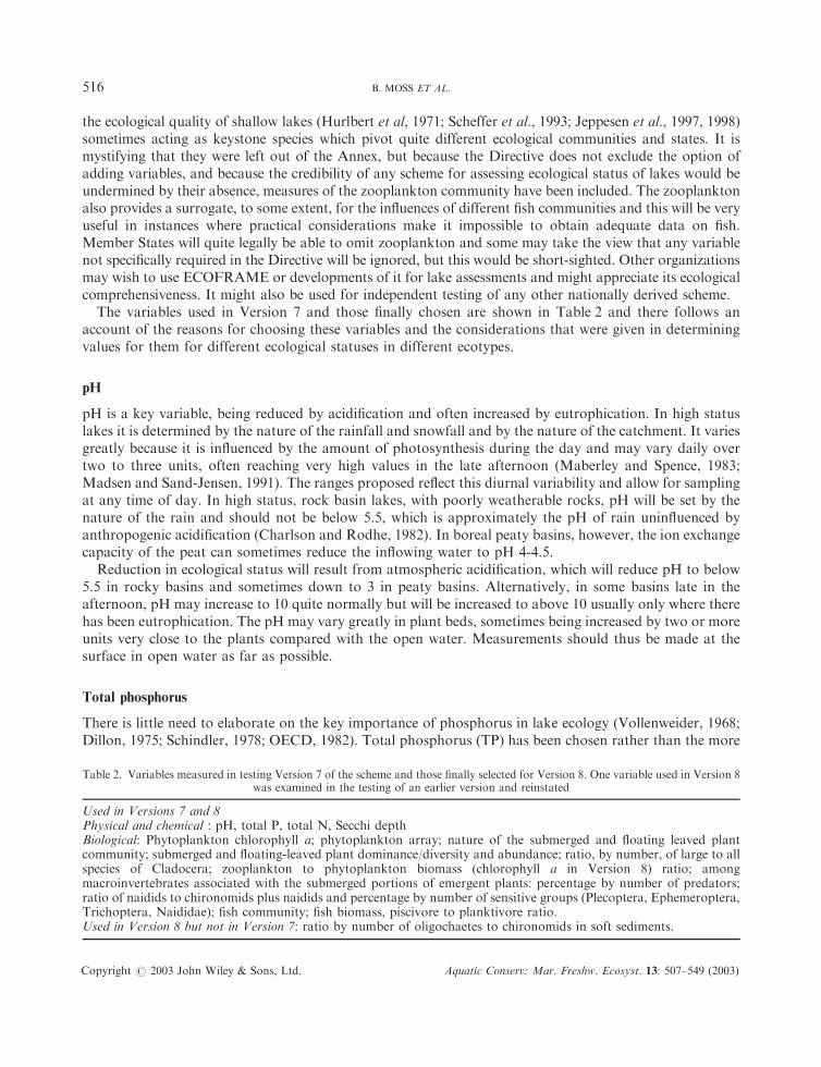
The variables used in Version 7 and those finally chosen are shown in Table 2 and there follows anaccount of the reasons for choosing these variables and the considerations that were given in determiningvalues for them for different ecological statuses in different ecotypes.

pH

pH is a key variable, being reduced by acidification and often increased by eutrophication. In high statuslakes it is determined by the nature of the rainfall and snowfall and by the nature of the catchment. It variesgreatly because it is influenced by the amount of photosynthesis during the day and may vary daily overtwo to three units, often reaching very high values in the late afternoon (Maberley and Spence, 1983;Madsen and Sand-Jensen, 1991). The ranges proposed reflect this diurnal variability and allow for samplingat any time of day. In high status, rock basin lakes, with poorly weatherable rocks, pH will be set by thenature of the rain and should not be below 5.5, which is approximately the pH of rain uninfluenced byanthropogenic acidification (Charlson and Rodhe, 1982). In boreal peaty basins, however, the ion exchangecapacity of the peat can sometimes reduce the inflowing water to pH 4-4.5.

Reduction in ecological status will result from atmospheric acidification, which will reduce pH to below5.5 in rocky basins and sometimes down to 3 in peaty basins. Alternatively, in some basins late in theafternoon, pH may increase to 10 quite normally but will be increased to above 10 usually only where therehas been eutrophication. The pH may vary greatly in plant beds, sometimes being increased by two or moreunits very close to the plants compared with the open water. Measurements should thus be made at thesurface in open water as far as possible.

Total phosphorus

There is little need to elaborate on the key importance of phosphorus in lake ecology (Vollenweider, 1968;Dillon, 1975; Schindler, 1978; OECD, 1982). Total phosphorus (TP) has been chosen rather than the more

Table 2. Variables measured in testing Version 7 of the scheme and those finally selected for Version 8. One variable used in Version 8was examined in the testing of an earlier version and reinstated

Used in Versions 7 and 8Physical and chemical : pH, total P, total N, Secchi depthBiological: Phytoplankton chlorophyll a; phytoplankton array; nature of the submerged and floating leaved plantcommunity; submerged and floating-leaved plant dominance/diversity and abundance; ratio, by number, of large to allspecies of Cladocera; zooplankton to phytoplankton biomass (chlorophyll a in Version 8) ratio; amongmacroinvertebrates associated with the submerged portions of emergent plants: percentage by number of predators;ratio of naidids to chironomids plus naidids and percentage by number of sensitive groups (Plecoptera, Ephemeroptera,Trichoptera, Naididae); fish community; fish biomass, piscivore to planktivore ratio.Used in Version 8 but not in Version 7: ratio by number of oligochaetes to chironomids in soft sediments.

B. MOSS ET AL.516


easily measurable soluble reactive phosphorus because of the lability and considerable day-to-dayvariability of the latter. TP also varies but with much less amplitude. It may temporarily increase afterheavy rain as suspended particles and soluble forms are washed into lakes or from resuspension on a windyday. It may also increase in summer as a result of release of phosphate from sediments under plant beds,even under good and possibly even high ecological status conditions.

Our values may be liberally high for truly high status conditions. They take account of the familiar(though judgementally derived) OECD (1982) ranges but eutrophication is now so widespread that we mayhave become inured to values that are generally high. More phosphorus is delivered to lakes fromcatchments that have weatherable, more calcareous rocks than those providing soft waters of lowconductivity, but some karst (limestone or chalk) lakes have values as low as those for soft waters. In lakesof low conductivity, acidification mobilizes aluminium and results in flocculation of phosphorus-containingparticles and precipitation of soluble phosphorus. The phosphorus concentrations to be expected in poorand bad acidified states in these lakes are thus lower than those expected of good to moderate status. Thefact that a given range can indicate high status under some conditions and bad status under others is dealtwith by use of conditional statements in Version 8.

Total nitrogen

Nitrogen is also widely recognized as a key nutrient but its available forms (mostly nitrate and ammonium)are very labile and do not lend themselves to classifications where sampling will be infrequent. In manylakes with high available nitrogen concentrations at the beginning of the growth season, values oftenbecome undetectable by mid-summer so the measurement of total nitrogen is proposed. Total nitrogenincludes not only inorganic nitrogen but also organic nitrogen, which may be equally as abundant and issometimes easily mineralized for growth by algae and plants. In high status lakes, little influenced byhuman activity, available nitrogen is very scarce. It is retained by the catchment vegetation and itscompounds denitrified in the catchment soils. As the remainder enters the lakes it is further denitrified ortaken up so that in pristine lake waters most of what is detected as total nitrogen is in particulate ordissolved organic form.

The values set for high status lakes are thus low but may still be too liberal. Nitrogen is readily increasedby human activities, both through disruption of the catchment vegetation and through atmosphericpollution. The thresholds for status categories lower than ‘high’ are thus also relatively low and take intoaccount the fact that macrophyte communities are very effective at uptake and denitrification. There is anargument that measuring both key nutrients is redundant and that measurement only of total P is sufficient.However, there are lakes that are naturally nitrogen limited and nitrogen may be more crucial in thedetermination of aquatic plant community diversity than total phosphorus. The two nutrients thus throwlight on different ecological characteristics.

Secchi depth

The Secchi depth is a very convenient summary of many features of lakes but needs to be used carefully as itreflects the effects both of phytoplankton and inorganic and detrital turbidity as well as dissolved colouredsubstances in the water. In shallow lakes of high status the water should be very clear, with a dearth ofsuspended particles and the bottom visible at least at the mean depth. However, in acid peaty waters, suchas are found in large areas of northern Europe, naturally occurring humic substances will reduce thetransparency and the values in the scheme reflect this. Humic substances are also frequent in more alkalinewaters but the very large concentrations emanating from acid peat are usually not found. In very largelakes, disturbance of bottom deposits will also tend to reduce Secchi disc transparency and allowance hasbeen made for this. In lakes forming immediately at the feet of glaciers that are melting back, there willnaturally be a very high turbidity from suspended clay. Such glacier-foot lakes are not included in this



scheme because they are essentially disturbed riverine sites that have not yet attained their stable ecologicalcharacteristics.

Reductions in status may arise from eutrophication which will decrease the Secchi disc transparency.Where macrophyte populations are still present, these effects will be minimized by a range of mechanismsassociated with maintenance of water clarity (Moss, 1999) and the Secchi disc transparency will changelittle. Only when the systems switch to phytoplankton dominance will there be a major decrease. Whereacidification occurs and aluminium is mobilized, flocculation will increase the Secchi disc transparency andthe water may be clearer at poor and bad status than it is at high status. Allowance is made for all of thesefactors in the scheme and because Secchi disc transparency is independently affected by several features, thethresholds of change have been kept to a minimum. In shallow clear-water lakes when the Secchi disc isvisible on the bottom, use of a small disc in a dark tube (Schnell’s tube) may be a useful alternative to adirect Secchi measurement, although the availability of a Schnell’s tube has not been assumed in thescheme.

Phytoplankton chlorophyll a

Nutrient availability and phytoplankton chlorophyll a concentration are closely related, but not perfectly,because of the influence of grazing, mixing and flushing in keeping chlorophyll concentrations below thepotential set by nutrient availability. Because natural catchment vegetation in pristine areas tends to retainnutrients within the terrestrial communities (Pennington, 1984), the availability of nutrients tophytoplankton communities of all pristine lakes is naturally low. Biomass of the communities, reflectedin chlorophyll a, will thus be low irrespective of the local geology, at high ecological status. Reduced statuswill result from increase in nutrient flow and increased chlorophyll a concentrations in all but some verysoft-water lakes. Such lakes may be influenced by eutrophication, especially from atmospheric sources ofnitrogen, but reduced status is more likely to be caused by acidification which will reduce the chlorophyll athrough flocculation.

It is conceivable that a soft-water lake may suffer both acidification (from the atmosphere) andeutrophication (for example from village or farm sewage) simultaneously, in which case almost anycombination of Secchi disc transparency, nutrients and chlorophyll could be found. Lakes in generallyacidified soft-water regions showing symptoms of eutrophication may show a higher status than justifiedbecause of the mutual interaction of acidification and eutrophication.

Phytoplankton community

There are many general predictions about the nature of phytoplankton communities in differentcircumstances (Rawson, 1956; Reynolds, 1984, 1987). They are perhaps the best understood of allcomponents of lake ecosystems. However, there is immense change in composition from week to week andthe time taken to determine the separate components of phytoplankton biomass is large. The rapidturnover of the phytoplankton community, coupled with the costs of the determination, make itinappropriate to specify great detail in any practicable scheme.

In Version 7, categories were confined to the presence of a multi-species community compared with anessentially monospecific one of Cyanobacteria or Chlorococcales and this distinction was used todiscriminate between poor and bad status when nutrients increase. Almost all lakes were expected to have,and did have, a multi-species community. In Version 8 this has been modified to use also observations ofsurface cyanobacterial blooms. Member States may wish to measure, for example, the proportion ofcyanophytes and other major groups of phytoplankton, but the patterns are not simply predictable. Aheavily eutrophicated system will not, for example, necessarily show large amounts of cyanophytes (Jensenet al., 1994), whereas a high status lake may have a high proportion of these algae at certain times(McGowan et al., 1999). Version 7 included, as part of the (more predictable) ratio of biomass of

B. MOSS ET AL.518


zooplankton to phytoplankton (McCauley and Kalff, 1981) a measure of total phytoplankton biovolume(see below) so that a method was developed for those competent authorities who might nonetheless wish touse components of the algal community. However, the time taken to make this estimate was very large,because of the need to measure cell size as well as cell count, and for Version 8 the ratio was converted toone of zooplankton biomass to chlorophyll a.

Plant and phytobenthos community

The submerged and floating-leaved plant/phytobenthos community, or its absence, is the key variable inshallow lakes as it determines much of the lake function (Jeppesen et al., 1998). Emergent macrophytes arealso important and included below under the criteria for nature of the shoreline. There are threecomponents to the assessment of the plant community: its general taxonomic status, diversity andabundance. The community is influenced in pristine conditions by the climate (through the length of thegrowing season), light penetration, the availability of sediment for colonization, which will tend to begreater in peaty and more calcareous basins, the nutrient status of the sediment and water, and theconductivity of the water. Six easily recognizable community categories have been defined (Appendix 1).

The presence of large amounts of humic substances, with their strong light-absorbing properties will tendto favour the taller-growing nymphaeid and canopy-forming communities in extreme cases, but in generalthe lower nutrient loading of high status conditions will be associated with low-growing communities ofsmall plants. Acidification will tend to displace these in favour of Sphagnum. In general, only very soft-waterlakes will be affected by acidification and all by eutrophication. Eutrophication will result in replacementwith taller, more competitive elodeids and pondweeds. Eventually only stands of plants with most of theirphotosynthetic tissue at the surface} nymphaeids, lemnids and canopy formers likeMyriophyllum spicatum} will be able to persist as potential periphyton and phytoplankton burdens increase.

Some existing schemes for assessing lake status use specific determinations of the plant community(Palmer et al., 1992). These require taxonomic expertise and a greater expenditure of time in sampling thanthe ecological community approach taken here. It is also not possible to specify unequivocally, particularspecies to particular states (Seddon, 1972), a problem that exists for all biological variables. There is muchstochastic substitution possible. However, one human impact on lakes is the introduction of some alienspecies of plants, which may suppress the diversity of the native flora. This has been built in toconsiderations of plant diversity (see below) but does require the recognition of these species.

Because of the importance of plants in shallow lakes, two further measures of the plant community areincluded to ensure that sufficient weighting is accorded to plants. These are plant diversity and plantabundance. Measures are designed to be quick and cheap. In early testing several person-days could beneeded for conventional estimates of macrophyte biomass. For Version 7 plant dominance was simplymeasured as multi-species or monospecies communities, but this was elaborated to predictions of totalnumber of species for Version 8.

The biomass of plants is an important consideration but large quantity is not synonymous with highstatus. A degree of eutrophication can produce dense beds that are less diverse in other organisms thansparser beds. Dense beds, for example, can produce overnight deoxygenation and fish kills. Abundance canbe measured precisely as PVI (percentage volume infested) but this takes a very long time to do properly. Arapid method was developed which involves inspection of an area about one tenth of that of the lake andsimple use of a rake or grapnel. The plants are scored as in Appendix 1.

Zooplankton ratios

Ratios have proved more useful than absolute measures of zooplankton communities and two were used.The first is the ratio of numbers of large species of Cladocera (Daphnia, Eurycercus, Simocephalus, Sida,Diaphanosoma, Holopedium, Leptodora, Polyphemus) to total numbers of Cladocera including the small



species (all others). The second is the ratio of crustacean zooplankton biovolume (or biomass) tophytoplankton biovolume (or biomass). To compromise between the expense of making thesemeasurements (which is very high) simple counts were used together with standard tables of averagebiovolume for each species derived from the literature. This gave adequate estimates for the zooplankters,despite the range of variation in size brought about through predation, but not for phytoplankters whichhad to be individually determined at the cost of much time. Consequently, for Version 8 a zooplanktonbiomass to chlorophyll a ratio has been specified.

In lakes at high ecological status, there is a larger proportion of large Cladocera, which find refuges fromfish predation among the plant communities. Where plants are lost (low quality states) in all lakes, largezooplankters become much less frequent. There are, however, indications that large species are relativelyless abundant in pristine warm lakes perhaps because of the multiple recruitment of small fish (Lazzaroet al., 1992; Lazzaro, 1997). The scheme recognizes these features.

The ratio of zooplankton biovolume to phytoplankton biovolume or chlorophyll a gives an independentmeasure of the influence of the zooplankton and also includes copepod zooplankton as well as cladoceranzooplankton. Inclusion of rotifers did not increase the usefulness of the ratio, but increased the costs ofdetermining it. Ratios tend to be high where the zooplankton community is supported by the refuges givenby the structure provided to the ecosystem by plants, which in turn tend to suppress phytoplanktonproduction through mechanisms which include maintenance of high numbers of large efficient grazerswithin these refuges.

Macroinvertebrates

Macroinvertebrate communities are very varied, not only between lakes but also within lakes. There aremany possible within-lake communities, but few that can be guaranteed to be present, for comparativepurposes, in all lakes. Sampling may be expensive because of the considerable heterogeneity of distributionof the animals. A range of different sorts of samplers, of different efficiencies and characteristics, may beneeded for particular conditions. Sediment is generally present in all lakes but may be sparse in the littoralzones of rocky basins. The sedimentary benthos has been used, historically, to characterize lakes (Berg,1938; Brinkhurst, 1974; Saether, 1979; Brinkhurst and Cook, 1980; Wiederholm, 1980; Bazzanti andSeminara, 1986; Johnson and Wiederholm, 1989). Many of these classifications depend on good taxonomicexpertise, though some are simple, but a great deal of time is usually needed for sorting the samples. Forother macroinvertebrate communities there are few systematic data that can be used to formulatehypotheses concerning relationships with other features in lakes. Though the Directive requires assessmentsof macroinvertebrates, the complexity of their communities and the variety of their habitats made their useextremely difficult in assessing ecological status.

Simplicity was considered desirable so this component was best assessed, not by using submerged plants,which might be absent, but by using the emergent macrophytes which fringe virtually all lakes to someextent. Their submerged stems can be easily sampled and the animals scraped off. Thereafter, because of thetaxonomic variety of the community, it became difficult to predict characteristics of ecological status at thegeneric or species level but, as with zooplankton ratios, using families and indicators of functional statusare probably most reliable.

Three such variables, derived from the invertebrate community of emergent macrophytes, were used: thepercentage of individuals of the family Orthocladiinae among the chironomid larvae present (in Version 7only); the ratio of numbers of the oligochaete Naididae to the sum of Naididae and total chironomids; thepercentage of predators among the assemblage; and the percentage of taxa (Plecoptera, Ephemeroptera,Trichoptera, Naididae) particularly sensitive to eutrophication and deoxygenation (Macan, 1963; Learneret al.,1978; Uzunov, 1982). The Orthocladiinae are characteristic of highly oxygenated waters and thus tendto reflect high status (Armitage et al., 1995), as does a high ratio of Naididae to chironomids. A greater

B. MOSS ET AL.520


proportion of invertebrate predators is expected in high status lakes, because of the refuge structure againstfish predation provided by the plants (Diehl and Kornij !oow, 1998). In high status lakes, abundance of fish isexpected to be low, thus minimizing fish predation pressure on larger invertebrates (Kajak et al., 1980),among which predators are prominent. In warm lakes these ratios tend to be reduced by the naturally loweroxygen content of such waters and this is reflected in the scheme.

The sorting of Orthocladiinae from other chironomids took an unacceptable length of time andsubstantial taxonomic expertise where small instars were present. The Orthocladiinae to total chironomidratio was thus discarded in Version 8. However, following discard at an earlier stage, the ratio ofoligochaetes (largely Tubificidae) to chironomids in soft sediment samples was reinstated. Partly this wasbecause all the ratios show considerable variation when only a limited number of samples can be taken,because of the extreme heterogeneity of animal distribution, so that the more ratios measured, the morelikely is the average picture to reflect ecological conditions. Partly it was because the long tradition of usingthis community in applied limnology (Chandler, 1970; Brinkhurst, 1974; Saether, 1979; Wiederholm, 1980)will result inevitably in a wish for its use by competent authorities, irrespective of need.

Fish community

The Directive specifically asks that information on the fish community be used. The fish community willneed to be specified locally because of the substantial biogeographic variation throughout Europe. Somelakes of high status will have no fish community because they have been isolated since the last glaciationand this will have to be determined locally. If there is a natural fish community, it should have certaingeneral characteristics at high status. There will be locally characteristic native piscivores present, eithersalmonid, percid or esocid, whilst aggressive introduced species (Pimental et al., 2001) will be absent. Thus,introductions of common carp (Cyprinus carpio } from Asia) (Cahn, 1929) or rainbow trout(Onchorhyncus mykiss } from North America) will downgrade the status of a site, as will introductionsof ruffe (Gymnocephalus cernua) from lowland to upland lakes within the UK or the introduction of thenon-native roach (Rutilus rutilus) to Irish lakes. Non-aggressive introductions, largely of curiosity value,such as those of the bitterling (Rhodeus sericeus) into the UK are not used to downgrade a site in thescheme. However, the long-term unpredictability of the damage caused by introduced species might promptcompetent authorities to downgrade a site if any introduced species are present. This issue is relevant also tointroduced plants and invertebrates.

Fish biomass

The former view that ‘the more fish the better’ is no longer consistent with an understanding of ecologicalquality. Fish can be extremely damaging either directly to macrophyte communities or indirectly throughtheir predation on zooplankton and plant-associated invertebrate grazers. Data are now available onthresholds of biomass likely to cause damage (Moss et al., 1996) and these have been used in the scheme, sothat decrease in quality is initially reflected in increased biomass. Total loss is also detrimental and mayoccur through acidification or nocturnal or sub-ice deoxygenation following eutrophication. In all cases theassumption is that fish would naturally be present in a lake but when the scheme is used in polar andmontane regions, recognition is built in that many lakes there are naturally fishless. The biomasses quotedare for the entire fish community, including the young of the year, which are often excluded from fisheryestimates. However, they may be very important, through their predation on zooplankton, for determiningecological status.

Fish piscivore to zooplanktivore ratio

This variable is valuable in itself but is also used as a surrogate for age distribution of the fish community,required by the Directive, which would otherwise be extremely difficult to specify in a usable way. It would



also be very expensive to determine, because several fish species are present in most lakes. High quality,clear shallow lakes are characterized by relatively high biomasses of piscivores, reflecting oxygenationconditions as well as complex ecosystem structure. Poor quality lakes lose their predators (Jeppessen et al.,1997) allowing major increases in zooplanktivores. These usually skew the size and age distribution rangetowards smaller and younger fish. The biomass ratio of piscivores to zooplanktivores is thus a very goodindicator of status. In warmer lakes, specialist piscivores may be scarcer, in favour of omnivores, and theratio has been set lower in these lakes, but values are less certain because of the limited number ofquantitative studies in such lakes. There may also be subtleties in the changes in acidified lakes because oflesser sensitivity of some piscivores to decreased pH. However, in the absence of comprehensive data sets,this has not been incorporated into the scheme.

Quantity and dynamics of water flow, residence time

The hydrology of a particular site will be unique to that site. It will depend on the local rainfall and itstiming and on the shape and size of the lake basin and the relative sizes of lake basin and catchment (theDirective uses the term ‘river basin’ instead of catchment, but catchment is used here to avoid confusion). Itis not possible to state positively what the characteristics will be, therefore, for each ecotype. This is aproblem for all the hydrological and morphological characteristics and some of the physico-chemicalfactors specified in Annex V of the Directive (Table 1). The problem can be solved by specifying absence ofrelevant impacts rather than absolute values of the variable.

The amount of water flow and the pattern in time in which it arrives, and hence the residence time, will allinfluence the ecology of a lake because they determine nutrient loading, the development of plankton, themaintenance of marginal fish spawning habitat and many other details of lake function. However, they alsonormally fluctuate to a considerable degree dependent on weather. There are notably dry and notably wetyears in most locations and the biota will have been selected to accommodate these. Weather also changessteadily owing to natural climate changes and, at present and more rapidly, to anthropogenic change.

Water flows, however, can be more seriously influenced by diversion of inflows to irrigation projects orabstraction for water supply and these can influence ecological status (Davies et al., 1992). Adding water, intransfer schemes for water supply, could also be ecologically damaging for it usually brings in water ofdifferent chemical nature and may introduce alien organisms. The scheme allows for the characteristics ofnatural variation and potentially damaging effects of abstraction or addition by using the categories shownin Appendix 1. The same characteristics are used for residence time because residence time is stronglydependent, for a given morphometry of the lake basin, on water flow into it.

Connection to groundwater

Many lakes are parts of groundwater systems and receive inflows from the groundwater or discharge to it.Again the degree of connection will depend on the local circumstances and is not specifiable on the basis ofecotype. However, lakes significantly fed by groundwater may be denied their natural supply if thegroundwater table is drawn down by abstraction for irrigation or water supply. The same terminology ofNormal, Modified and Severely modified as for surface water hydrology is used with the definitions shownin Appendix 1.

Lake depth variation

Lake depth variation can be taken to mean either lake level variation or characteristics of the profile of thebasin. The former usage is covered under the hydrological characteristics above and it is the lattercharacteristic that is considered here. The profile of the basin is determined by the way that it was originally

B. MOSS ET AL.522


formed coupled with subsequent sedimentation. The former determinant is lake-specific and cannot bespecified on an ecotype basis.

Sedimentation is also naturally lake-specific, depending on the nature of the catchment, but can beinfluenced by human activities resulting in increased erosion of the catchment or increased in-lakeproduction of sediment because of eutrophication. Change in sedimentation rate in sediment cores couldthus be used as an index of ecological quality. The annual deposition should be low and approximatelyconstant under high ecological status and would increase with most sorts of human activity.

Determining sedimentation rate is, however, very expensive, requiring coring and dating of the coredsediment. It does not lend itself to routine use. This characteristic is thus best measured indirectly(Appendix 1). Increased sedimentation almost always results from disturbance of the catchment byagriculture and hence the degree of conversion of the landscape to agriculture has been used as a measure.In this, grazing means intense pasture usage with fertilization and ploughing to create productive swards.Extensive grazing in unfenced, unfertilized pastures (as long as stocking levels have not been excessive inresponse to headage payment schemes) is considered to be much less damaging (Hornung et al., 1984). Suchan interpretation of this variable also allows the important consideration of how the catchment has beenmodified to be reinforced.

Quantity, structure and substrate of the lake bed

This characteristic is also lake-specific and must be assessed by degree of disturbance. Lake beds may be ofa variety of particle sizes, or rocky. They may be covered with emergent or submerged macrophytes. Thelatter characteristic is already being measured by the macrophyte community. In some disturbed lakes,sedimentation may occur and may, for example, cover gravel spawning sites for salmonid fish. Alteration oflake levels by abstraction or water transfer may also lead to erosion or exposure of the littoral sediments.This is covered by the above hydrological assessments.

However, sands or gravels or rocks and boulders may be removed from some lakes for provision ofbuilding aggregate or horticultural purposes (garden design features) and this will have adverse effects. Thesubstrata removed may be highly specific and have a substantial effect on fish spawning. The allowablelevels of disturbance (Appendix 1) are thus quite low because even 1% of the lake area may be a substantialproportion of a particular critical substratum type. There may also be instances of dumping of soil or othermaterials into lakes as a result of road or other building activities. These too are allowed for in the scheme.

Structure of the lake shore

Lake shores are very varied and may include erosional bare shores and sheltered shores colonized bysequences of emergent and floating-leaved plants. There are many ecological interactions between thesefringing wetlands and the open water, shown by chemical patterns, migrations of organisms and nestingand lurking sites for birds, both grazers and piscivores, that influence the open water communities.

The pattern is lake-specific and cannot be specified for ecotypes but again this characteristic can beassessed by degree of disturbance. Lake shores may be cleared for urban, marina, or angling development,and damaged by boating activity or feral grazing birds. There may also be invasions of exotic species } forexample, Japanese knotweed (Fallopia japonica), giant hogweed (Heracleum mantegazzianum) orHimalayan balsam (Impatiens glandulifera). Shores may sometimes be concreted, or artificial beachesmay be created by dumping sand. Some shores are modified as gardens and lawns fringe the water.

High ecological status will be marked by natural shores. Where wind fetch prevents sediment deposition,the shores will be rocky, gravelly or sandy but they will have some vegetation, even if it is only sparseisoetids or algal phytobenthos. On depositional shores there will normally be emergent vegetation,sometimes low growing carices or rushes, sometimes tall reeds (Phragmites, Typha, Scirpus, Cladium,Schoenoplectus), sometimes woodland of willow (Salix), alder (Alnus), birch (Betula) or spruce (Picea) or a



variety of other species in warmer regions. It should nonetheless be easy to recognize naturally colonizedshores, to perceive development and severe damage and to identify the rather vigorous introduced species.The assessment is thus made by the proportion of the shoreline occupied by development, or by damagedvegetation, or by alien plants (Appendix 1).

Temperature

Temperature regimes of lakes depend on the local climate, with considerable year-to-year variation withchanges in weather. This is recognized in use of climate regions to provide the broad division of ecotypesthat simplifies the typology. It is, however, not possible to specify precise local conditions except on anindividual lake basis. Temperature can, however, be damaging where warm water is discharged from powerstations. It is conceivable also that in volcanic areas like Iceland, diversion of thermal streams or springsfrom a lake basin for domestic heating purposes might result in a deviation from the natural thermal statusof a particular lake. To allow for these possibilities the scheme uses categories (Appendix 1) that mirrorthose used for other locally-determined variables.

Oxygen

Oxygen concentration is of considerable significance in determining the nature of freshwater ecosystems.Oxygen is a highly labile substance, which varies greatly in concentration during the day and night andspatially within the water body, either as a result of natural temperature stratification or the complexpatterns of water chemistry created by the growth of plants. Sometimes oxygen concentrations will fall tonear zero in the lower parts of plant beds in lakes considered to have good ecological status.

A single measurement of oxygen as part of a lake survey is meaningless and proper characterizationwould require many measurements } spatial, diurnal and seasonal. Thus, although it would theoreticallybe possible to specify an oxygen regime for the different ecological states of each ecotype, it would be veryexpensive to determine as part of routine monitoring. However, the oxygen regime is a function of thenutrient supply and plant and algal growth and is indirectly specified by these variables in the scheme. Whatmay nonetheless happen is that there are discharges of deoxygenating substances like raw sewage or animalslurry. This is more usual in rivers and streams but may occasionally occur in lakes. Its effects areincorporated by use of the categories in Appendix 1.

Salinity

Salinity is a measure of the total salts in the water and high salinities may be natural. There are categories oftransitional waters and coastal waters in the Directive that reflect this. Fresh waters are conventionallyconsidered to have salinities lower than 0.5 g total salts per litre, with mixtures of sea water and fresh waterhaving larger values than this being considered brackish and falling into the transitional category. Thereare, however, waters close to the sea coast, with natural groundwater supplies of sea water, that do not fitthe category of transitional waters, and inland saline waters in dry regions where closed basin (endorheic)lakes occur. These may be quite saline because of evaporation but with a salt composition that is differentfrom that of sea water. Such lakes are usually small. To allow for these possibilities categories of lakes areincluded in the typology with conductivities greater than 800 mS cm�1.

There may, however, be pollution by salinity where sea water or industrial discharges enter lakes as aresult of human activities. For example, pumped drainage of catchments close to the sea may suck sea waterinto the groundwater table and then discharge it into the lake, increasing the salinity quite considerably andhaving major ecological effects (Holdway et al., 1978; Bales et al., 1993). Equally it is conceivable that theremay be diversions of fresh water for irrigation schemes that reduce the salinity of endorheic or coastal lakesbelow that which would be expected naturally. The reverse may occur where water is denied because of use

B. MOSS ET AL.524


for irrigation elsewhere, a common problem in Mediterranean regions. These possibilities have beenallowed for by designation of the categories in Appendix 1.

Pollution by priority substances

Priority substances are potentially listed in Annex X of the Directive but none has so far been designated.Criteria for ecological status have thus not been determined but would follow those for pollutantsubstances listed in Annex VIII.

Pollution by other substances

Annex VIII of the Directive lists pollutant categories as follows: organohalogens, organophosphoruscompounds, organotin compounds, carcinogens, mutagens and endocrine disruptors, persistent hydro-carbons and bioaccumulative organic toxins, cyanides, metals (presumed heavy) and their compounds,arsenic and its compounds, biocides and plant protection products, suspended material, eutrophicatingsubstances and deoxygenating substances. Annex V gives guidance on the limits to be applied to thesesubstances.

The cases of eutrophicating substances, deoxygenating substances and suspended solids have alreadybeen incorporated under the headings of total P, total N, oxygen and Secchi disc transparency. For theremainder, there exists a very long list of potential pollutants, many of which may be present from diffusesources rather than overt discharges. Annex V states that for high status these substances should be presentat close to zero concentrations, that are lower than the limits of detection of the most advanced techniquesin use. For good ecological status, their concentrations should be lower than that determined as a ‘noobservable effect concentration’ (NOEC), scaled down by safety factors, by procedures detailed in Section1.2.6 of Annex V.

These definitions cause a problem in that eutrophicating substances, deoxygenating substances, manyheavy metals, and suspended solids are features of natural systems uninfluenced by humans. Indeed some ofthese substances are absolutely required by living organisms and the conditions stipulated in Annex V,Section 1.2.6, would mean that no ecosystem could exist. This is clearly an oversight in the drafting of theDirective and conditions for these substances have been dealt with in the scheme in such a way as to takeaccount of this. For substances not falling into this category (recognized toxic pollutants) the scheme usesthe stipulations of the Directive. However, the determination of the NOEC for representative species ofeach ecotype poses a major problem for competent authorities and some general compromise will benecessary, perhaps by using the lowest NOEC concentrations determined for any system in the firstinstance. The case of the heavy metals is particularly difficult as many of these are required metabolites andsensitivities to them cover a wide range. The pollutant substances are dealt with collectively in the scheme(Appendix 1).

METHODS FOR SCHEME TESTING

Common protocols for all sampling and analysis were agreed and established as far as possible. Allsampling was carried out in late summer. Because the aim of the Water Framework Directive is to usebiological variables to the greatest extent, summer sampling is mandatory but chemical variables werechosen that might be expected to vary least over the year, for example total phosphorus and nitrogen asopposed to available forms of these nutrients.

Six lakes were chosen from each of 11 countries (see Table 3) to give a range in each country frompresumed high/good status to poor status based on experience from previous testing. The sample is thus notrepresentative of the average state of Europe’s lakes but includes about equal numbers of perceived high/



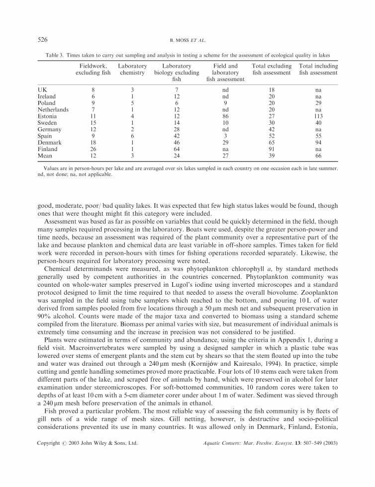
good, moderate, poor/ bad quality lakes. It was expected that few high status lakes would be found, thoughones that were thought might fit this category were included.

Assessment was based as far as possible on variables that could be quickly determined in the field, thoughmany samples required processing in the laboratory. Boats were used, despite the greater person-power andtime needs, because an assessment was required of the plant community over a representative part of thelake and because plankton and chemical data are least variable in off-shore samples. Times taken for fieldwork were recorded in person-hours with times for fishing operations recorded separately. Likewise, theperson-hours required for laboratory processing were noted.

Chemical determinands were measured, as was phytoplankton chlorophyll a, by standard methodsgenerally used by competent authorities in the countries concerned. Phytoplankton community wascounted on whole-water samples preserved in Lugol’s iodine using inverted microscopes and a standardprotocol designed to limit the time required to that needed to assess the overall biovolume. Zooplanktonwas sampled in the field using tube samplers which reached to the bottom, and pouring 10L of waterderived from samples pooled from five locations through a 50 mm mesh net and subsequent preservation in90% alcohol. Counts were made of the major taxa and converted to biomass using a standard schemecompiled from the literature. Biomass per animal varies with size, but measurement of individual animals isextremely time consuming and the increase in precision was not considered to be justified.

Plants were estimated in terms of community and abundance, using the criteria in Appendix 1, during afield visit. Macroinvertebrates were sampled by using a designed sampler in which a plastic tube waslowered over stems of emergent plants and the stem cut by shears so that the stem floated up into the tubeand water was drained out through a 240 mm mesh (Kornij !oow and Kairesalo, 1994). In practice, simplecutting and gentle handling sometimes proved more practicable. Four lots of 10 stems each were taken fromdifferent parts of the lake, and scraped free of animals by hand, which were preserved in alcohol for laterexamination under stereomicroscopes. For soft-bottomed communities, 10 random cores were taken todepths of at least 10 cm with a 5-cm diameter corer under about 1m of water. Sediment was sieved througha 240 mm mesh before preservation of the animals in ethanol.

Fish proved a particular problem. The most reliable way of assessing the fish community is by fleets ofgill nets of a wide range of mesh sizes. Gill netting, however, is destructive and socio-politicalconsiderations prevented its use in many countries. It was allowed only in Denmark, Finland, Estonia,

Table 3. Times taken to carry out sampling and analysis in testing a scheme for the assessment of ecological quality in lakes

Fieldwork,excluding fish

Laboratorychemistry

Laboratorybiology excluding

fish

Field andlaboratory

fish assessment

Total excludingfish assessment

Total includingfish assessment

UK 8 3 7 nd 18 naIreland 6 1 12 nd 20 naPoland 9 5 6 9 20 29Netherlands 7 1 12 nd 20 naEstonia 11 4 12 86 27 113Sweden 15 1 14 10 30 40Germany 12 2 28 nd 42 naSpain 9 6 42 3 52 55Denmark 18 1 46 29 65 94Finland 26 1 64 na 91 naMean 12 3 24 27 39 66

Values are in person-hours per lake and are averaged over six lakes sampled in each country on one occasion each in late summer.nd, not done; na, not applicable.

B. MOSS ET AL.526


Sweden, Spain and Poland, all countries with long traditions of consumption of freshwater fish. A standardprotocol was used with 42m� 1.5 or 0.75m monofilament nylon nets comprising 14 mesh sizes in 3-msection Lundgren nets. Mesh sizes ranged from 6.25 to 100mm. Nets were set close to shore and in mid-lakewith the number of nets proportional to lake area, up to a maximum of eight nets. In Finland and Poland30m x 1.5m monofilament nylon nets with 12 mesh sizes (5-55mm) in 2.5m sections were used (Nordicnets). Nets were set in late afternoon and retrieved the following morning. Double fyke nets, 10m long withcod ends of mesh size 8 and 5mm, were also used for benthic fish species. Catches were expressed as weightof fish caught per net-night.

In other countries, where fish are seen mainly in recreational angling terms, fish biomass could not bereliably measured, other methods such as seining being considered too unreliable, but information on fishcommunity composition was obtained from such methods and from local knowledge.

There is an additional problem in that gill netting gives estimates in terms of catch per unit effort(CPUE), whilst the ecologically meaningful unit is absolute biomass per unit area. Calibration of CPUE isdifficult. Criteria in Version 8 of the scheme are given in absolute biomass terms and it is accepted thatvalues for this variable will be crude. This will be either because inefficient fishing methods that are capableof giving a weight per unit area value have been used, or because gill netting results can only be converted toabsolute measures by comparison with these less efficient measures. Unfortunately, gill netting hence offersno advantage unless the fishing effort can be rigorously standardized and criteria in the scheme expressedonly as standardized CPUE. However, multiple mesh-sized gill netting, in such conditions, is by far the bestmethod to obtain an overview of the fish community composition and size distribution.

RESULTS

Times taken to accomplish the field and laboratory work in testing Version 7 are shown in Table 3. Thesetimings do not include travel between the base laboratory and the lake, which might add several person-hours. Fieldwork, excluding that required for fishing, averaged 12 person-hours, with a wide variation,from 4-26. This reflects largely the size of lake, because logistics and boat crew size are greater for largerlakes as is also the time taken to examine the 10% area required for plant assessment. Laboratorychemistry, averaging 3 person-hours, ranged from 1-6. To some extent, this reflected differences amonglaboratories where a routine system for handling many water samples was available and those where thesystem had to be established for this project.

Biological analyses (average 24 person-hours per lake) took from 6 to 64 person-hours. To some extentthis reflects difference in the richness of samples, but is mostly due to some laboratories having standardand very thorough procedures for biological analyses and being unable to reduce these standards in theinterests of practicability. It also reflects degrees of experience among the personnel used, sometimesrelatively inexperienced graduate students, sometimes technical staff with considerable knowledge. Many ofthese factors will also be present among the laboratories of competent authorities operating such schemes,so that the overall average for non-fish work of 39 person-hours or just over a standard person-week, isprobably realistic for operational purposes.

Estimates for the time taken for fisheries work, available from five of the countries, varied nearly tenfold,again reflecting the number of persons necessary on different-sized lakes and the need in some cases to postguards overnight against theft of nets. On average, fish work alone took almost as long as all other work inthe assessments, giving a final estimate of about 2 person-weeks to carry out the assessment on a singleoccasion. However, provisions of the Directive are that chemical assessments must be carried out at 3-month intervals, and phytoplankton at 6-month intervals. This will increase the time required to assess thequality of a lake by up to a further 45 person-hours, giving a total of 118 person-hours (about 3 person-weeks) per lake. In the initial determination of lake status for the Directive, an investment of the time of



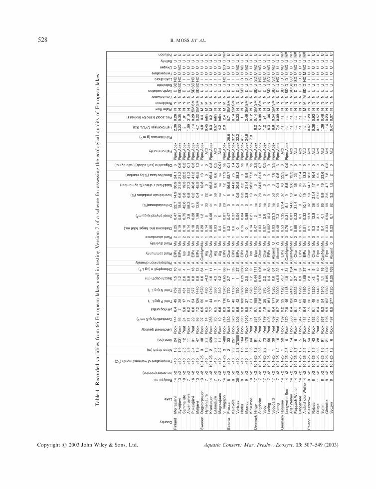
Table4.Recorded

variablesfrom

66Europeanlakes

usedin

testingVersion7ofaschem

eforassessingtheecologicalquality

ofEuropeanlakes

Fin

land

Mer

rasj

ärvi

14>

2>

101.

824

Roc

k14

46.

449

759

1.5

10A

ElP

oM

u2

0.25

0.47

22.7

14.9

30.9

24.1

3P

ipre

,Abe

x2.

360.

26N

NN

DS

DH

DU

UU

US

ylvö

järv

i13

>2

>10

1.9

231

Roc

k92

738

634

1.2

6A

ElP

oM

u1

0.19

0.81

18.5

6.6

21.9

21.3

0.6

Pip

re,A

bex

3.22

0.35

NN

NS

DS

DH

DU

MD

UU

Sam

mal

isto

10>

2>

102.

512

Pea

t24

5.6

1748

12.

64

AIs

oM

u2

0.16

0.75

42.6

3.8

19.3

22.5

0.2

Pip

re,A

bex

21.

01N

NN

DU

IU

UU

UA

hven

lam

mi

7>

2>

103.

911

Roc

k21

6.2

223

75.

81

AIs

oM

u2

0.14

2.8

58.3

6.8

37.3

41.3

0.1

Pip

re,A

bex

1.09

31.9

NN

NU

UI

UU

UU

Puk

alaj

ärvi

16>

2>

102.

431

Pea

t29

6.6

5467

70.

818

AE

lPo

Mo

10.

180.

283.

70.

240

.841

.20.

3P

ipre

,Abe

x1.

140.

29S

MS

MN

SD

SD

HD

UU

UU

Mat

järv

i13

>2

>10

1.5

47R

ock

967.

212

614

400.

812

AE

lPo

Mu

20.

291.

9812

.60.

445

.945

.51.

3P

ipre

,Abe

x4.

70.

22S

MS

MN

SD

SD

HD

UU

UU

Sw

eden

Dag

stor

pssj

on13

<2

10.1

-25

348

Roc

k97

6.5

5015

700.

664

AC

anN

ymM

u 1

0.28

1.2

44

12.8

134

Pip

re,A

bex

4.8

0.4

MM

NU

UI

UU

UU

Hym

enja

ure

7>

2>

101.

32.

2R

ock

146.

58

430

>4.

21

AA

lgM

o1

0.14

833

220

00

Altd

0.45

infin

MM

NU

UI

UU

UU

Kra

nkes

jon

14<

210

.1-2

52

420

Roc

k28

67.

744

1210

1.6

11A

Cha

rM

u3

0.05

0.06

418

65.3

65.4

0.3

Pip

re,A

bex

8.3

0.2

MM

NU

UI

UU

UU

Lass

ejau

re7

>2

>10

3.7

3.2

Roc

k20

6.5

935

04.

31

AA

lgM

u1

0.03

30

598.

68.

60.

5A

ltd0.

57in

finN

NN

UU

IU

UU

UM

agnu

sjau

re7

>2

>10

2.2

1.4

Roc

k10

6.6

734

04.

21

AA

lgM

o1

0.4

5na

nana

na0.

01A

ltd4.

2in

finN

NN

UU

IU

UU

UV

. Rin

gsjo

n14

<2

10.1

-25

314

80R

ock

214

8.9

110

1370

0.65

66A

ElP

oM

u1

0.01

0.01

297

1217

.9na

Pip

re,A

bex

2.9

2.4

MM

ND

UH

DU

SD

UM

PE

ston

iaP

ross

a8

>2

>10

233

Roc

k33

08.

417

770

2.7

7A

Cha

rM

u4

0.2

0.47

06

56.5

52.7

0.1

Pip

re,A

bex

28.6

0.71

SM

SM

ND

UI

UU

UU

Kai

aver

e8

>2

>10

2.2

251

Roc

k37

08.

343

1150

135

AE

lPo

Mu

10.

60.

370

444

.875

1.4

Pip

re,A

bex

37.2

0.14

SM

SM

ND

UI

UU

UU

Vor

tsja

v26

>2

>10

2.8

2700

0R

ock

306

8.6

4275

01

27A

ElP

oM

u1

00.

040

0.5

20.5

38.2

0.4

Pip

re,A

bex

32.2

0.23

NN

ND

UI

UM

DU

UH

arku

8>

2>

101.

616

4R

ock

290

9.8

186

2760

0.25

230

AE

lPo

Mu

20.

150.

040

3.3

3.2

3na

Pip

re,A

bex

41.1

1N

NN

SD

UD

UM

DU

UM

aard

u9

>2

>10

1.6

170

Roc

k10

108.

527

780

2.5

10A

Cha

rM

u3

00.

880

2.8

21.4

9.9

naP

ipre

,Abe

x24

.82.

46S

MS

MN

DU

DU

MD

UU

Kiri

kum

ae10

>2

>10

2.8

64P

eat

217.

521

670

1.2

9A

Iso

Mu

10.

140.

210

1398

.277

.5na

Pip

re,A

bex

7.9

0.12

NN

ND

UD

UU

UU

Den

mar

kH

inge

17<

210

.1-2

51.

291

Pea

t33

19.

118

814

700.

4411

1A

Elp

oM

u1

0.47

3na

00

02.

5P

ipre

,Abe

x6.

20.

14S

MS

MN

SD

US

DU

MD

UU

Stig

shol

m17

<2

10.1

-25

0.8

21P

eat

276

8.9

316

1270

0.59

106

AC

har

Mo

10.

031.

6na

2034

.931

.90.

7P

ipre

,Abe

x5.

20.

98N

SM

ND

UH

DU

MD

UU

Sob

y17

<2

10.1

-25

2.8

73P

eat

179

7.9

2837

52.

28

AC

har

Mu

20.

072.

6na

00

00.

5P

ipre

,Abe

x1.

224

NN

ND

UH

DU

UU

ULa

ding

17<

210

.1-2

51

56P

eat

493

8.1

161

1300

0.4

80A

ElP

oM

o1

0.00

210

.3na

00

00

Pip

re,A

bex

8.3

1.06

MN

NS

DU

SD

UM

DU

US

obyg

ard

17<

210

.1-2

51

39P

eat

469

8.4

171

1525

0.6

61A

Abs

ent

O0

0.03

23.3

na53

37.

83.

5P

ipre

,Abe

x8.

80.

54S

MS

MN

SD

US

DU

MD

UU

Vae

ng17

<2

10.1

-25

1.2

16P

eat

281

8.7

7920

00>

0.9

22A

Abs

ent

O0

0.48

7.3

na20

0.4

0.5

3P

ipre

,Abe

x7.

40.

09N

NN

DU

HD

UU

UU

Ger

man

yR

ohrs

ee14

<2

10.1

-25

150

Roc

k13

99.

239

1126

>1.

74

AE

lPo

Mu

40.

531.

3527

.437

4322

.50

Altd

nana

NN

NS

DD

DU

MD

UM

PLe

ngw

eile

r S

ee14

<2

10.1

-25

2.8

6R

ock

370

7.9

4511

181.

931

AC

anN

ymM

o3

0.76

0.31

5.1

95.

58

0.9

Pip

re,A

bex

nana

NN

NS

DD

DU

MD

UM

PA

lter

Wei

her

14<

210

.1-2

51.

314

Roc

k55

88.

412

624

100.

713

4A

Can

Nym

Mo

20.

10.

0114

.613

2.6

12.3

0A

ltdna

naN

NN

SD

SD

SD

UD

CM

PF

lapp

ach

Weh

er14

<2

10.1

-25

3.7

6R

ock

454

8.1

1339

223.

75

AC

har

Mu

20.

850.

2331

.46

3523

0A

ltdna

naN

NN

DD

SD

UM

DU

MP

Lang

ense

e14

<2

10.1

-25

1.7

5R

ock

347

7.9

6312

280.

937

AE

lPo

Mu

30.

150.

10

2586

37.4

0A

ltdna

naN

NN

DD

DU

DU

MP

And

elsh

ofer

Wei

he14

<2

10.1

-25

2.5

37R

ock

431

8.4

6911

601.

0537

AE

lPo

Mu

10.

010.

3210

.119

2413

.30

Altd

nana

MM

MS

DD

HD

MM

DU

MP

Pol

and

Kle

szcz

ow8

>2

10.1

-25

1.3

54R

ock

117

7.5

3610

802.

84

AC

har

Mu

30.

113

.982

1914

.718

.20

Altd

0.67

1.29

NN

NU

UI

UU

UU

Rot

cze

8>

210

.1-2

51.

943

Roc

k15

29.

149

1220

>3

5A

Cha

rM

u3

0.3

12.8

3821

.417

16.4

0A

ltd0.

380.

93N

NN

UU

IU

UU

UD

lugi

e11

>2

10.1

-25

0.8

28P

eat

129

8.4

5614

40>

0.8

12A

Elp

oM

u3

0.4

3.1

6627

.28

5.5

0A

ltd0.

110.

57N

NN

UU

IU

UU

US

umin

8>

210

.1-2

51.

691

Roc

k36

78.

354

1340

1,1

16A

Can

Nym

Mu

10.

44.

165

9.9

1923

.60

Altd

1.36

0.46

NN

NU

UI

UU

UU

Gle

boki

e8

>2

10.1

-25

3.4

21R

ock

198

9.9

102

1350

0.85

102

AE

lpo

Mu

10.

330.

5488

3.5

4.7

7.8

0.3

Altd

1.14

0.23

NN

NU

UI

UU

UU

Syc

zyn

8>

210

.1-2

51.

26

Roc

k49

78.

527

721

200.

2516

3B

Abs

ent

00

0.23

0.1

823.

21.

52

0A

ltd0.

470.

07N

NN

UU

IU

UU

U

Pollution

Country

Water flow

Residence

Groundwater

Depth variation

Substrate

Lake shore

Temperature

Oxygen

Salinity

Fish ommunity

Fish biomass (g m-2)

Pisc:zoopl (ratio by biomass)

Fish biomass CPUE (kg)

Invertebrate predators (%)

Naid:Naid + chiro (% by number)

Sensitive taxa (% by number)

Oligo:chiro [soft substr] (ratio by no.)

Plant abundance

Cladocera (no. large: total no.)

Zoopl:phytopl (µg:µm3)

Orthocladineae(%)

Chlorophyll a (µg L-1)

Phytoplankton diversity

Plant community

Plant diversity

pH (log units)

Total N (µg L-1)

Total P (µg L-1)

Secchi depth (m)

Mean depth (m)

Area (ha)

Catchment geology

Conductivity (µS cm-2)

Lake

Ecotype no.

Ice cover (months)

Temperature of warmest month (°C)

B. MOSS ET AL.528


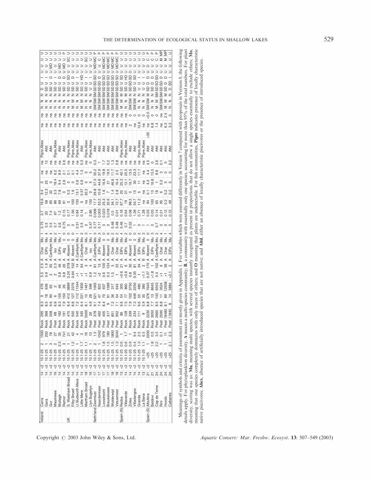
Irel

and

Car

ra14

<2

10.1

-25

215

00R

ock

295

8.3

947

65.

52.

5A

Cha

rM

u1

0.75

3.7

16.6

9.4

0na

naP

ipre

,Abe

xna

naN

NN

DU

IU

UU

UG

ara

14<

210

.1-2

51

202

Roc

k36

88.

518

636

0.9

1.9

AE

lPo

Mu

40.

520

5812

.325

na13

Altd

nana

NN

NS

DU

IU

UU

UG

ur14

<2

10.1

-25

378

Roc

k20

89.

690

652

65A

Can

Nym

Mu

40.

57.

485

320

nana

Altd

nana

NN

NS

DU

DU

MD

UU

Mau

mw

ee16

<2

10.1

-25

227

Pea

t68

6.8

62

22.

3A

Iso

Mu

20.

767

863.

318

.46.

2na

Pip

re,A

bex

nana

NN

NS

DU

IU

UU

UM

ulla

gh14

<2

10.1

-25

2.3

35R

ock

182

8.3

105

460.

846

AE

lPo

Mu

10.

61.

269

7.8

9.4

8.9

naA

ltdna

naN

NN

SD

UD

UM

DU

UR

amor

14<

210

.1-2

53

741

Roc

k19

17.

915

026

0.8

26A

Alg

00

0.75

0.15

910

2.6

2.1

0.6

Altd

nana

NN

NS

DU

DU

MD

UP

UK

S. W

alsh

am B

road

14<

210

.1-2

51

21R

ock

475

8.4

412

3889

0.24

378

AA

bsen

t0

00

0.17

00.

50

0.1

naP

ipre

,Abe

xna

naN

NN

SD

US

DU

US

CU

Filb

y B

road

14<

210

.1-2

51.

242

Roc

k50

08.

812

723

760.

6410

2B

Abs

ent

00

01.

5610

01.

60

0.1

naP

ipre

,Abe

xna

naM

MN

SD

UD

UU

UU

Lt B

udw

orth

Mer

e14

<2

10.1

-25

14

Roc

k54

07.

211

211

544

>1

14A

Can

Nym

Mu

10.

510.

8410

013

.10.

64.

4na

Pip

re,A

bex

nana

NN

NS

DU

IU

UU

ULi

ttle

Mer

e14

<2

10.1

-25

1.7

3R

ock

345

6.4

331

1830

>1

64A

Can

Nym

Mu

20.

50.

140

0.57

0.6

1.3

0.3

Altd

nana

MM

NS

DU

HD

UU

UU

Mar

tham

Bro

ad18

<2

10.1

-25

1.1

16R

ock

5000

8.1

1014

61>

13

AC

har

Mu

30

1na

32.2

00

naP

ipre

,Abe

xna

naN

NN

SD

UI

UU

SC

ULl

yn B

ugei

lyn

16<

210

.1-2

51

13P

eat

264.

928

598

0.9

4A

Iso

Mu

10.

472.

8610

00

55

0P

ipre

,Abe

xna

naN

NN

UU

IU

UU

UN

eth'

land

Zw

emlu

st17

<2

10.1

-25

21.

5P

eat

378

9.1

521

1065

1.2

61A

Can

Nym

Mo

30.

770.

008

17.7

29.8

57.3

35.2

0.3

Altd

nana

SM

SM

SM

SD

SD

SD

UM

DM

CP

Naa

rder

mee

r17

<2

10.1

-25

110

42P

eat

492

7.4

4782

2>

213

AE

lPo

Mu

30.

110.

003

53.2

10.6

44.8

37.9

1A

ltdna

naS

MS

MS

MS

DS

DD

UU

CP

Loos

drec

ht17

<2

10.1

-25

1.8

979

Pea

t40

58.

470

937

0.6

100

AA

bsen

t0

00

0.02

325

.31.

616

.619

.81.

7A

ltdna

naS

MS

MS

MS

DS

DS

DU

MD

MC

PB

reuk

elve

en17

<2

10.1

-25

1.5

180

Pea

t31

79

9115

890.

312

4A

Abs

ent

00

00.

018

32.6

721

19.5

0.2

Altd

nana

SM

SM

SM

SD

SD

SD

UM

DM

CP

Wol

derw

ijd18

<2

10.1

-25

1.5

1800

Pea

t85

17.

236

317

1.5

5A

Cha

rM

o2

0.48

0.5

34.1

1.4

46.6

11.7

1.3

Altd

nana

SM

SM

SM

SD

SD

SD

UM

DM

CP

Vel

uwm

eer

18<

210

.1-2

51.

332

40P

eat

952

7.1

5464

51

22A

Cha

rM

o2

0.48

0.01

72.7

2.8

16.4

2.3

0.8

Altd

nana

SM

SM

SM

SD

SD

SD

UM

DM

CP

Spa

in (

N)R

edos

13<

210

.1-2

50.

61

Roc

k86

9.6

5430

0>

0.6

21A

ElP

oM

u4

0.46

0.18

67.7

2025

.340

.1na

Pip

re,A

bex

nana

MM

MS

DU

SD

UU

UU

Vill

aver

de14

<2

10.1

-25

0.6

1.7

Roc

k12

87.

577

860

>0.

66

AE

lPo

Mu

20.

70.

6419

2112

.125

.5na

Pip

re,A

bex

nana

NN

MS

DU

HD

UU

UU

Zot

es14

<2

10.1

-25

0.9

1R

ock

339

7.9

102

3750

0.8

30A

Abs

ent

00

0.02

0.08

98.5

016

.713

.5na

Altd

20

SM

SM

NS

DS

DS

DD

UU

UV

illad

ango

s14

<2

10.1

-25

0.4

9.4

Roc

k23

47.

344

622

500.

3581

AA

bsen

t0

01

1.28

54.7

1530

23.3

naA

ltdna

0S

MS

MN

SD

US

DU

UU

UG

rand

e14

<2

10.1

-25

1.3

2.5

Roc

k11

19.

655

480

134

AE

lPo

Mu

20

0.71

11.2

511

11.1

naP

ipre

,Abe

x12

.60

NN

NU

UI

UU

UU

La B

ana

13<

210

.1-2

51.

16.

5R

ock

95.

930

380

>1.

12

BE

lPo

Mu

31

1.28

nana

nana

naP

ipre

,Abe

xna

0N

NN

UU

IU

UU

US

pain

(S

)A

lbuf

era

21<

2>

251

2200

Roc

k22

308.

837

676

450.

3717

0A

Abs

ent

00

10.

0394

0.1

4.3

4.4

4.5

Altd

>30

na<

0.5

SM

SM

MS

DD

DU

DC

PB

aldo

vi21

<2

>25

1.8

0.5

Roc

k30

507.

713

8645

>1.

81

AE

lPo

Mu

30

0.03

100

1316

.813

.50

Altd

6.8

0N

NN

SD

DD

UU

CP

Cap

de

Tem

e24

<2

>25

2.2

3.5

Pea

t26

608.

514

065

530.

410

2A

Can

Nym

Mu

20.

70.

1465

181

8.8

3.6

Altd

1.4

0M

MS

MS

DS

DS

DU

UC

PR

ini

24<

2>

251

0.1

Pea

t25

908.

811

3524

>1

6A

Cha

rM

u4

00.

2195

60.

23

0.1

Altd

nana

SM

SM

SM

SD

SD

DU

UM

MP

Hon

do24

<2

>25

111

Pea

t18

480

8.1

8912

938

>1

36A

Cha

rM

u1

00.

120.

20.

20

00

Altd

6.3

2.4

MM

MS

DD

DU

UM

MP

Cab

anes

24<

2>

252.

12.

3P

eat

1184

08

1458

84>

2.1

2A

ElP

oM

u4

00.

1249

0.2

00

0.2

Altd

3.3

0N

NN

DS

DI

UU

UU

Meaningsofsymbolsandcriteria

ofassessm

entare

mostly

given

inAppendix

1.Forvariableswhichwereassesseddifferentlyin

Version7comparedwithproposalsin

Version8,thefollowing

detailsapply.Forphytoplanktondiversity,Ameansamulti-speciescommunity;B,acommunitywithessentiallyonly

onespecies,accountingformore

than95%

ofthetotalnumbers.Forplant

diversity,scoringwasas:

Mu,meaningmultispecies,

withseveralspeciesinstantlyrecognized

aspresentin

proportionsthatdonotallow

asingle

speciesessentiallyto

excludeothers;

Mo,

meaningthatonespeciescompletely

dominateswithonly

tracesofothers;andO

meaningthatplants

are

indetectable.Forfish

communities,Pipre

indicatespresence

oflocallycharacteristic

nativepiscivores;

Abex,absence

ofartificiallyintroducedspeciesthatare

notnative;

andAltd,either

anabsence

oflocallycharacteristicpiscivoresorthepresence

ofintroducedspecies.



more than 60 people per 1000 lakes examined per year might be expected. Surveillance and restorationoperations will keep at least this number of people employed subsequently. It should be remembered thatthis scheme is a minimalist one, its components being much less complicated than many procedurescurrently being examined by competent authorities. However, the time investment needed is likely to besubstantially greater than that involved in current monitoring in some States.

Data obtained for the 66 European lakes are shown in Table 4. There were examples from 13 of the 48possible ecotypes, with a dearth of large lakes. This reflects the prominence of small lakes in Europe as awhole. Among the smaller lakes there were examples from half the possible ecotypes. Assessments ofecological status have been made based on these data using Version 7 of the scheme. This differs in manydetails from Version 8 given in the Appendix, but not so greatly that most assessments would besubstantially altered. In making assessments, the highest possible status was ascribed where the value of avariable would fit more than one category.

Table 5 shows correlations among numerical variables in the data in Table 4. It confirms that there islittle redundancy in the measures used, for most are not significantly correlated. The exception is the groupof variables linked through phytoplankton production and the results here are as expected. Totalphosphorus is linked with chlorophyll and negatively with Secchi disc depth and plant abundance.Chlorophyll is positively correlated with pH and negatively with Secchi transparency. Plant abundance isrelated to Secchi transparency. Correlations between chemistry and invertebrate indicators are few andisolated, suggesting that these are measuring independent properties of the ecosystem.

Assessments of quality were made in several ways. One interpretation of the Directive is that to attain agiven status, all variables must meet that standard (Environment Agency, 2002). Hence we have assessedthe lakes on this criterion of 100% compliance (Table 6). This is undoubtedly unrealistic, because of highnatural variability in most characteristics, but raises the issue of what proportion of individual variablesmust fall into a particular category or better for a given status to have been achieved. Logic suggests thatthis should not be lower than half, so this has been used as a criterion in Table 6 also. Half, however, is nota particularly stringent criterion, so assessments have also been included where 75% of the variables have toachieve a particular status or better for the lake to be given that status. In all cases we have calculated the

Table 5. Relationships among numerical variables obtained from 66 European lakes.Values are correlation coefficients

TP TN Secchi Cphyll Plantabund

Zoopllge:total

Zoopl:phytop

Orthocl(%)

Predat(%)

Naidids(%)

Sensits(%)

oligo:chiro

pH ns ns �0.35* 0.33* ns ns ns ns ns ns ns nsTP �0.52*** 0.63*** �0.35** 0.26* ns ns ns ns ns nsTN 0.36** ns ns ns ns ns ns ns �0.27* nsSecchi �0.54*** 0.32* ns ns ns ns ns ns nsCphyll �0.41** ns ns ns ns ns �0.27* nsPlant abund ns ns ns ns ns ns nsZoopl lge: total ns ns ns ns ns nsZoopl: phytop ns ns ns ns 0.49**Orthocl (%) ns ns ns nsPredat (%) ns ns nsNaidids (%) 0.39** nsSensits (%) ns ns

* p50.05, ** p50.01, *** p50.01; ns, not significant. Abbreviations: TP, total phosphorus concentration; TN, total nitrogenconcentration; Secchi, Secchi disc transparency; Cphyll, chlorophyll a concentration; Plant abund, Plant abundance; Zoopl lge:total,ratio of numbers of large (>0.5mm) Cladocera to total Cladocera; Orthocl (%), Orthocladiniiae as percentage of total chironomidnumbers; Predat, predators as a percentage of total macroinvertebrates; Naidids, Naididae as a percentage of total numbers ofchironomids plus Naididae; Sensits, percentage of sensitive taxa (Naididae, Ephemeroptera, Plecoptera, Trichoptera) of total numberof macroinvertebrates; oligo:chiro, ratio of numbers of oligochaetes to numbers of chironomids in soft sediments.

B. MOSS ET AL.530


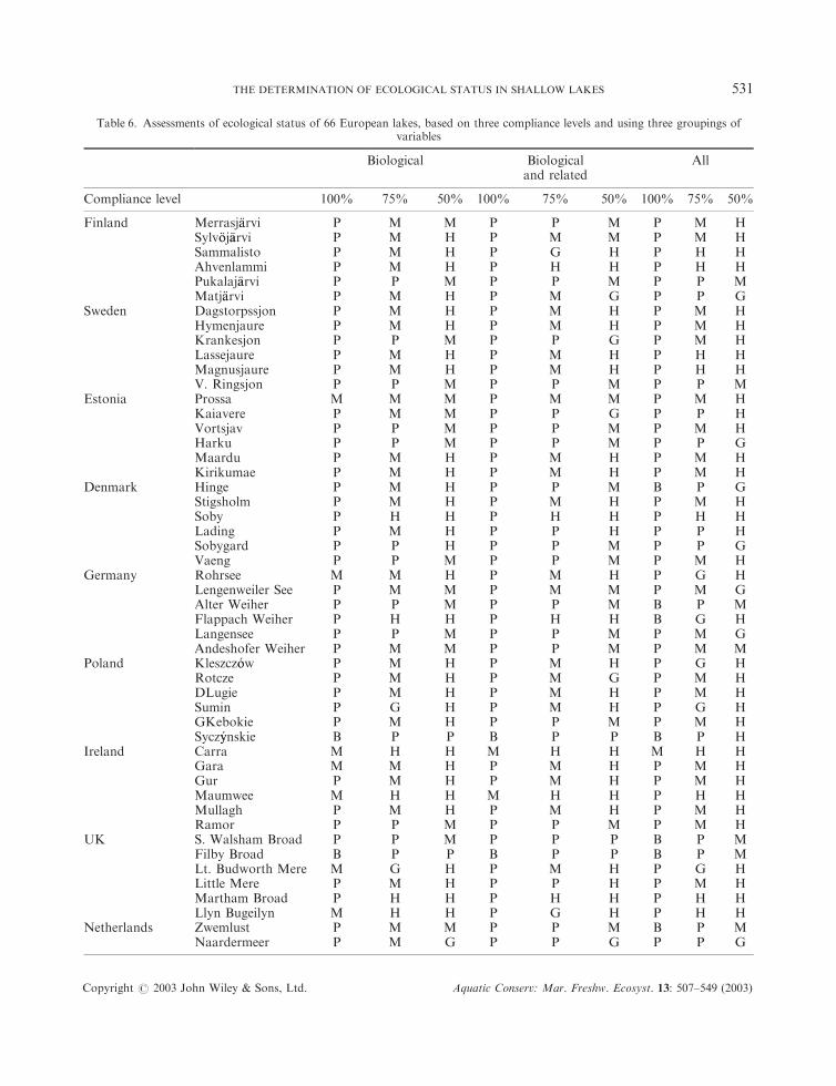
Table 6. Assessments of ecological status of 66 European lakes, based on three compliance levels and using three groupings ofvariables

Biological Biologicaland related

All

Compliance level 100% 75% 50% 100% 75% 50% 100% 75% 50%

Finland Merrasj.aarvi P M M P P M P M HSylv .ooj.aarvi P M H P M M P M HSammalisto P M H P G H P H HAhvenlammi P M H P H H P H HPukalaj.aarvi P P M P P M P P MMatj.aarvi P M H P M G P P G

Sweden Dagstorpssjon P M H P M H P M HHymenjaure P M H P M H P M HKrankesjon P P M P P G P M HLassejaure P M H P M H P H HMagnusjaure P M H P M H P H HV. Ringsjon P P M P P M P P M

Estonia Prossa M M M P M M P M HKaiavere P M M P P G P P HVortsjav P P M P P M P M HHarku P P M P P M P P GMaardu P M H P M H P M HKirikumae P M H P M H P M H

Denmark Hinge P M H P P M B P GStigsholm P M H P M H P M HSoby P H H P H H P H HLading P M H P P H P P HSobygard P P H P P M P P GVaeng P P M P P M P M H

Germany Rohrsee M M H P M H P G HLengenweiler See P M M P M M P M GAlter Weiher P P M P P M B P MFlappach Weiher P H H P H H B G HLangensee P P M P P M P M GAndeshofer Weiher P M M P P M P M M

Poland Kleszcz !oow P M H P M H P G HRotcze P M H P M G P M HDLugie P M H P M H P M HSumin P G H P M H P G HGKebokie P M H P P M P M HSycz!yynskie B P P B P P B P H

Ireland Carra M H H M H H M H HGara M M H P M H P M HGur P M H P M H P M HMaumwee M H H M H H P H HMullagh P M H P M H P M HRamor P P M P P M P M H

UK S. Walsham Broad P P M P P P B P MFilby Broad B P P B P P B P MLt. Budworth Mere M G H P M H P G HLittle Mere P M H P P H P M HMartham Broad P H H P H H P H HLlyn Bugeilyn M H H P G H P H H

Netherlands Zwemlust P M M P P M B P MNaardermeer P M G P P G P P G



assessment based on the total number of variables for which data were available. In many cases fishbiomass data and piscivore to zooplanktivore ratios were not available.

The Directive also indicates that water bodies should be classified according to ecological status andphysical and chemical status and that the final classification shall be determined by the lesser of the two.Assessments here are based on strict ecological status using only biological variables and also on all thevariables combined. Assessments are also made on a compromise group which included the strictlybiological variables (chlorophyll, macrophytes, phytoplankton, zooplankton, macroinvertebrates, fish)together with those that are so closely related as to be ecologically inseparable (pH, TP, TN, Secchi depth,shoreline structure). Thus Table 6 includes nine possible assessments for each lake. These data aresummarized as frequency distributions in Table 7. The distributions can be compared with the expecteddistribution of around one third each of the lakes in each of the groups high/good, moderate and poor/bad.Prior expectations were for 23 high/good, 21 moderate and 22 poor/bad lakes, which is very close to a 1:1:1ratio.

Using a criterion of 100% compliance among all variables, no lakes would be classed as high or good,rather few as moderate and most as poor or bad. Clearly this deviates markedly from expectation (Chisquared test for ratio of high/good : moderate : poor/bad, w2 ¼ 17:8, df ¼ 1, p50.01). Equally, using 50%compliance, a very high proportion emerges as high/good and many fewer as moderate or poor/bad. This isequally deviant (w2 ¼ 13:7, df ¼ 1, p50.01). A closer fit (w2 ¼ 4:0, df ¼ 1, ns) is realized with 75%compliance, though with fewer than notionally expected in the high/good categories. Few of the lakes couldtruly be said to be at high status based on the Directive’s very stringent definition, yet 13.6% fell into thiscategory at the 75% compliance level. This level therefore represents perhaps a less than stringent choice,and operationally perhaps a level of 80% compliance might be more appropriate.

Table 6 (continued)

Biological Biologicaland related

All

Compliance level 100% 75% 50% 100% 75% 50% 100% 75% 50%

Loosdrecht P P P P P P B P PBreukelveen P P P P P P B P PWolderwijd M M H P M H B P GVeluwmeer P M H P M H B P M

Spain (N) Redos P M H P M H B M HVillaverde M M H P M H P M HZotes P P M P P P B P PVilladangos P P M P P M B P MGrande P M M P M M P M HLa Bana B M M B M G B M H

Spain (S) Albufera P P M P P M P P MBaldovi P P G P P G P M HCap de Terme P P H P P M B P MRini M M H P M H P P GHondo P P H P P G P M GCabanes P P M P P M P M H

At the 100% compliance level, all variables had to meet the requirements stipulated for a particular status class or a higher one. For75% compliance at least three quarters had to meet the requirements for a particular class or a higher class and similarly for the 50%compliance level. Biological variables included chlorophyll a, phytoplankton community, and all variables concerned with plants,zooplankton, macroinvertebrates and fish, where available. Biologically related variables included pH, total P, total N, Secchi disctransparency and structure of the lake shore. H, high; G, good; M, moderate; P, poor; B, bad.

B. MOSS ET AL.532


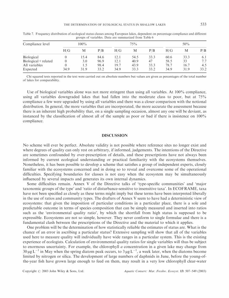
Use of biological variables alone was not more stringent than using all variables. At 100% compliance,using all variables downgraded lakes that had fallen into the moderate class to poor, but at 75%compliance a few were upgraded by using all variables and there was a closer comparison with the notionaldistribution. In general, the more variables that are incorporated, the more accurate the assessment becausethere is an inherent high probability that, on a single sampling occasion, almost any one will be deviant, asinstanced by the classification of almost all of the sample as poor or bad if there is insistence on 100%compliance.

DISCUSSION

No scheme will ever be perfect. Absolute validity is not possible where reference sites no longer exist andwhere degrees of quality can only rest on arbitrary, if informed, judgements. The intentions of the Directiveare sometimes confounded by over-prescription of details, and these prescriptions have not always beeninformed by current ecological understanding or practical familiarity with the ecosystems themselves.Nonetheless, it has been possible to develop a scheme that satisfies a group of independent experts, closelyfamiliar with the ecosystems concerned and in doing so to reveal and overcome some of the operationaldifficulties. Specifying boundaries for classes is not easy when the ecosystem may be simultaneouslyinfluenced by several impacts and generates its own internal dynamics.

Some difficulties remain. Annex V of the Directive talks of ‘type-specific communities’ and ‘majortaxonomic groups of the type’ and ‘ratio of disturbance-sensitive to insensitive taxa’. In ECOFRAME, taxahave not been specified as closely as these terms might imply but these terms have been interpreted liberallyin the use of ratios and community types. The drafters of Annex V seem to have had a deterministic view ofecosystems: that given the imposition of particular conditions in a particular place, there is a sole andpredictable outcome in terms of species composition that can be simply measured and inserted into ratiossuch as the ‘environmental quality ratio’, by which the shortfall from high status is supposed to beexpressible. Ecosystems are not so simple, however. They never conform to single formulae and there is afundamental clash between the prescriptions of the Directive and the material to which it applies.

One problem will be the determination of how statistically reliable the estimates of status are. What is thechance of an error in ascribing a particular status? Extensive sampling will show that all of the variablesused here to measure quality will individually have wide ranges in a particular system. This is the existingexperience of ecologists. Calculation of environmental quality ratios for single variables will thus be subjectto enormous uncertainty. For example, the chlorophyll a concentration in a given lake may change from30 mgL�1 in May when the spring diatom peak occurs, to 3 mgL�1, a week later, when the diatoms becomelimited by nitrogen or silica. The development of large numbers of daphnids in June, before the young-of-the-year fish have grown large enough to feed on them, may result in a very low chlorophyll clear-water

Table 7. Frequency distribution of ecological status classes among European lakes, dependent on percentage compliance and differentgroups of variables. Data are summarized from Table 6

Compliance level 100% 75% 50%

H/G M P/B H/G M P/B H/G M P/B

Biological 0 15.4 84.6 12.1 54.5 33.3 60.6 33.3 6.1Biological+related 0 3.0 96.9 12.1 40.9 47 58.5 33 7.7All variables 0 1.5 98.4 19.7 43.9 33.3 78.7 16.7 4.5Expected 34.9 31.9 33.2 34.9 33.3 33.2 34.9 31.9 33.2

Chi squared tests reported in the text were carried out on absolute numbers but values are given as percentages of the total numberof lakes for comparability.



phase which is replaced a week later by a major peak as the young fish decimate the zooplankton. In asingle lake during the summer, therefore, the entire range specified for different statuses can be met.

Calculation of environmental quality ratios is also impossible where qualitative features such as thenature of the plant community are concerned, yet these are among the most important measures ofecological quality. The assumptions of Annex V of the Directive seem to be that impacts on the systems arereflected in a simple proportional change in a constant set of taxonomic components. This is clearly neverthe case; the system changes to reflect the impact, acquiring new species by colonization and losing some bylocal extinction.

Collectively, however, the use of 28 variables will give a much more reliable way of expressingenvironmental quality ratios in terms of the number of variables attributable to particular classes. It is notpossible to say how reliable without wider-scale testing, but multiple sampling on single sites, andapplication of the assessment on each occasion, will be able to show probabilities of obtaining particularclasses. Data on multiple sampling of pond mesocosms (McKee et al., 2002) indicates that such an exercisewould show very high reliability if based on the entire suite of variables or a substantial majority of them.

An alternative approach is to regard the percentage of variables falling into a particular status class as ameasure of reliability that that status is the true assessment, or alternatively the number of variables fallinginto a given or higher status. This latter is the approach taken in Tables 6 and 7. Expectations of 100%compliance or 50% compliance are unreliable, but 75% compliance gave a pattern that was notsignificantly different from that expected from the choice of sites. Use of percentage compliance thus allowsan assessment of the risk of misclassification to be made. This might be done by regarding the percentage ofvariables falling into a particular class or a higher one as the probability of the lake falling into that class ora higher one. More sophisticated assessments could give different weightings to some variables comparedwith others.

A further approach might be to evaluate the amalgamated percentage compliance across a set of lakes ina given ecotype in a particular River Basin District (the management unit for the Water FrameworkDirective). This would minimize the risk of misclassification of a particular water body owing to stochasticfactors but assumes that all examples of an ecotype in the District are subject to similar impacts. This mayoften be the case, but not always.

Extension of the scheme to all lakes

The Water Framework Directive ultimately has to be applied to all lakes, not just shallow ones. There aretwo obvious differences between shallow lakes as discussed here and deeper lakes. First, the predominanceof bottom primary production is lost to predominance by phytoplankton in a deeper lake simply as afunction of availability of the two sorts of habitat. Second, the water mass will be more likely to stratify,with the possibility that the chemical nature of the water in the hypolimnion will change markedly fromthat in the epilimnion. There is a common presumption that the degree of deoxygenation of thehypolimnion will reflect ecological quality. A reduction from that in the pristine state will certainly indicatethis, but in absolute terms a deoxygenated hypolimnion may be pristine if the volume of the hypolimnion issmall in relation to that of the epilimnion. It is a lake-specific feature and thus cannot be built into a qualityscheme except in the way that ECOFRAME deals with other lake-specific features (see Appendix 1).

In other respects a deep lake will behave much as a shallow one, though the seasonal dynamics of manyvariables will differ owing to the effects of stratification. The scheme developed reflects the ecology of alllakes. In the interests of usability, two possibilities might be suggested. The simplest is that depth is ignoredas a variable in the typology and that samples be taken from epilimnion water and sediments where the lakestratifies, and that the scheme simply be applied to all lakes in the next stage of operational testing. Minoradjustment would be needed to the stipulations for macrophyte coverage to allow for the fact that much ofa deep lake might be unavailable for macrophyte colonization.

B. MOSS ET AL.534


However, Annex II of the Directive implies that depth is a mandatory component of typologies. Thus wesuggest a simple creation of two depth categories, 53m and >3m mean depth, and a simple replication ofthe 48 ecotypes of the present shallow lakes scheme with the characteristics of ecological quality unchanged,except for the proviso concerning macrophyte coverage discussed above.

A final observation

During the workshop discussions of this project, one of us remarked that from a single visit to a lake, anoverview of its catchment, knowledge of its pH and Secchi disc transparency, and a brief examination of itsmacrophytes, an experienced limnologist could easily distinguish high/good from moderate from poor/badstatus. It is the tragedy of our time, perhaps of all times, that we must set up expensive and elaboratemeasures to do what, with experience, and consensus within society as to its environmental goals, could bedone much more easily.

ACKNOWLEDGEMENTS

This work was supported by a Framework 5 contract from the European Commission (ECOFRAME, ContractEVK1–CT1999-00039). LAH was also supported from Swedish MISTRA funds through the VASTRA programme,and EJ and JPJ by the Danish Nature and Forest Agency. We are grateful for very helpful editorial and refereecomments made by Dr P. Boon and Dr C. Duigan.

REFERENCES

Armitage PD, Cranston PS, Pinder, LCV (eds) 1995. The Chironomidae. Biology and Ecology of Non-Biting Midges.Chapman and Hall: London.

Bales M, Moss B, Phillips G, Irvine K, Snook D. 1993. The changing ecosystem of a shallow, brackish lake, HicklingBroad, Norfolk, UK. II. Long-term trends in water chemistry and ecology and their implications for restoration ofthe lake. Freshwater Biology 29: 141–166.

Bazzanti M, Seminara M. 1986. Profundal macrobenthos structure as a measure of long-term environmental stress in apolluted lake. Water, Air and Soil Pollution 33: 435–442.

Bennion H, Juggins S, Anderson NJ. 1996. Predicting epilimnetic phosphorus concentrations using an improveddiatom-based transfer function and its application to lake eutrophication management. Environmental Science andTechnology 30: 2004–2007.

Bennion H, Wunsam S, Schmidt R. 1995. The validation of diatom-phosphorus transfer functions: an example fromMondsee, Austria. Freshwater Biology 34: 271–283.

Berg K. 1938. Studies on the bottom animals of Esrom Lake. Danske Videnskabers Selskab Skrift 7:1–255.Blindow I. 1992. Decline of charophytes during eutrophication: comparison with angiosperms. Freshwater Biology 28:1–14.

Boon PJ. 2000. The development of integrated methods for assessing river conservation value. Hydrobiologia 422:413–428.

Brinkhurst RO. 1974. The Benthos of Lakes. Macmillan: London.Brinkhurst RO, Cook DG (eds). 1980. Aquatic Oligochaete Biology. Plenum: New York.Cahn AR. 1929. The effect of carp on a small lake: the carp as a dominant. Ecology 10: 271–274.Chandler JR. 1970. A biological approach to water quality management. Water Pollution Control 69:415–422.

Charlson RJ, Rodhe H. 1982. Factors controlling the acidity of natural rainwaters. Nature 295: 683–685.Davies BR, Thoms M, Meador M. 1992. An assessment of the ecological impacts of inter-basin transfers, and theirthreats to river basin integrity and conservation. Aquatic Conservation: Marine and Freshwater Ecosystems 2:325–350.

Diehl S, Kornij !oow R. 1998. The influence of macrophytes on trophic interactions among fish and macroinvertebrates.In The Structuring Role of Submerged Macrophytes in Lakes, Jeppesen E, S�ndergaard M, S�ndergaard M,Christoffersen K. (eds). Springer Verlag: New York; 24–46.



Dillon PJ. 1975. The application of the phosphorus-loading concept to eutrophication research. Environment CanadaScience Series 46, Burlington: Ontario.

Environment Agency. 2002. The Water Framework Directive. Guiding Principles on the Technical Requirements.Environment Agency: Bristol.

Hansson L-A, Annadotter H, Bergman E, Hamrin SF, Jeppesen E, Kairesalo T, Luokkanen E, Nilsson PA,S�ndergaard M, Strand J. 1998. Biomanipulation as an application of food-chain theory: constraints, synthesis andrecommendations for temperate lakes. Ecosystems 1: 558–574.

Holdway PA, Watson RA, Moss B. 1978. Aspects of the ecology of Prymnesium parvum (Haptophyta) and waterchemistry in the Norfolk Broads, England. Freshwater Biology 8: 295–311.

Hornung M. 1984. The impact of upland pasture improvement on solute outputs in surface waters. In Agriculture andthe Environment, Jenkins D (ed.). Institute of Terrestrial Ecology: Cambridge; 150–155.

Hurlbert SH, Zedler J, Fairbanks D. 1971. Ecosystem alteration by mosquito fish (Gambusia affinis) predation. Science175: 639–641.

Hynes HBN. 1970. The Biology of Polluted Waters. Liverpool University Press: Liverpool.Irvine K, Moss B, Balls HR. 1989. The loss of submerged plants with eutrophication. II Relationships between fish andzooplankton in a set of experimental ponds, and conclusions. Freshwater Biology 22: 89–107.

Jensen JP, Jeppesen E, Olrik K, Kristensen P. 1994. Impact of nutrients and physical factors on the shift fromcyanobacterial to chlorophyte dominance in shallow Danish lakes. Canadian Journal of Fisheries and Aquatic Sciences51: 1692–1699.

Jeppesen E, Leavitt P, De Meester L, Jensen JP. 2001a. Functional ecology and palaeolimnology: using cladoceranremains to reconstruct anthropogenic impact. Trends in Ecology and Evolution 19: 191–198.

Jeppesen E, Jensen JP, S�ndergaard M, Lauridsen T, Landkildehus F. 2001b. Trophic structure, species richness andbiodiversity in Danish lakes: changes along a phosphorus gradient. Freshwater Biology 45: 201–218.

Jeppesen E, Jensen JP, S�ndergaard M, Lauridsen T, Pedersen LJ, Jensen L. 1997. Top-down control infreshwater lakes: the role of nutrient state, submerged macrophytes and water depth. Hydrobiologia 342/3:151–164.

Jeppesen E, Madsen, EA, Jensen, JP, Anderson NJ. 1996. Reconstructing the past density of planktivorous fish andtrophic structure from sedimentatry zooplankton fossils: a surface sediment calibration data set from shallow lakes.Freshwater Biology 36: 115–127.

Jeppesen E, S�ndergaard M, Kronvang B, Jensen JP, Svendsen LM, Lauridsen TL. 1998. Lake and catchmentmanagement in Denmark. Hydrobiologia 395/396: 419–432.

Jeppesen E, S�ndergaard M, Mortensen E, Kristensen P, Riemann B, Jensen HJ, M .uuller JP, Sortkj!ccr O, Jensen JP,Christoffersen K, Bosselmann S, Dall E. 1990. Fish manipulation as a lake restoration tool in shallow, eutrophictemperate lakes 1: cross-analysis of three Danish case studies. Hydrobiologia 200/201: 205–218.

Jeppesen E, S�ndergaard M, S�ndergaard M, Christoffersen K (eds). 1998. The Structuring Role of SubmergedMacrophytes in Lakes. Ecological Studies, vol 131, Springer Verlag: New York.

Johnes PJ. 1996. Evaluation and management of the impact of land use change on the nitrogen and phosphorus loaddelivered to surface waters: the export coefficient modelling approach. Journal of Hydrology 183: 323–349.

Johnes PJ, Moss B, Phillips GL. 1996. The determination of water quality by land use, livestock numbers andpopulation data } testing of a model for use in conservation and water quality management. Freshwater Biology 36:451–473.

Johnson R, Wiederholm K. 1989. Classification and ordination of profundal macroinvertebrate communities innutrient poor, oligo-mesohumic lakes in relation to environmental data. Freshwater Biology 21: 375–386.

Kajak Z, Bretschko G, Schiemer F, Leveque C. 1980. Zoobenthos. In The Functioning of Freshwater Ecosystems, LeCren ED, Lowe-McConnell RH (eds). Cambridge University Press: Cambridge; 285–307.

Kristensen P, Hansen HO. 1994. European Rivers and Lakes. Assessment of their Environmental State. EEAEnvironmental Monographs, vol 1. European Environment Agency: Copenhagen.

Kornij !oow R, Kairesalo T. 1994. A simple apparatus for sampling epiphytic communities associated with emergentmacrophytes. Hydrobiologia 294: 141–143.

Lazzaro X. 1997. Do the trophic cascade hypothesis and classical biomanipulation approaches apply to tropical lakesand reservoirs? Verhandlungen der Internationalen Vereinigung f .uur theoretische und angewande Limnologie 26:719–730.

Lazzaro X, Drenner RW, Stein R.A, Smith JD. 1992. Planktivores and plankton dynamics - effects of fish biomass andplanktivore type. Canadian Journal of Fisheries and Aquatic Sciences 49: 1466–1473.

Learner MA, Lochhead G, Hughes BD. 1978. A review of the biology of British Naididae (Oligochaeta) with emphasison the lotic environment. Freshwater Biology 8: 357–375.

B. MOSS ET AL.536


Maberley SC, Spence DHN. 1983. Photosynthetic inorganic carbon use by freshwater plants. Journal of Ecology 71:705–724.

Macan TT 1963. Freshwater Ecology. Longman: London.McCauley E, Kalff J. 1981. Empirical relationships between phytoplankton and zooplankton biomass in lakes.Canadian Journal of Fisheries and Aquatic Sciences 38: 458–463.

McGowan S, Britton G, Haworth E, Moss B. 1999. Ancient blue-green blooms. Limnology & Oceanography 44:436–439.

McKee D, Atkinson D, Collings S, Eaton J, Harvey I, Heyes T, Hatton K, Wilson D, Moss B. (2002) Macro-zooplankter responses to simulated climate warming in experimental freshwater microcosms. Freshwater Biology 47:1557–1570.

Madsen TV, Sand-Jensen K. 1991. Photosynthetic carbon assimilation in aquatic macrophytes. Aquatic Botany 41:5–40.

Makarewicz JC, Likens GE. 1975. Niche analysis of a zooplankton community. Science 190: 1000–1002.May RM. 1977. Thresholds and breakpoints in ecosystems with a multiplicity of stable states. Nature 269:471–477.

Moss B. 1999. From algal culture to ecosystem, from information to culture. European Phycological Journal 34:193–204.

Moss B, Kornijow R, Measey GJ. 1998. The effects of nymphaeid (Nuphar lutea L.) density and predation by perch(Perca fluviatilis L.) on the zooplankton communities in a shallow lake. Freshwater Biology 39: 689–697.

Moss B, Johnes PJ, Phillips GL 1997. New approaches to monitoring and classifying standing waters. In FreshwaterQuality: Defining the Indefinable?, Boon PJ, Howell DL (ed.). The Stationery Office: Edinburgh; 118–133.

Moss B, McGowan S, Carvalho L. 1994. Determination of phytoplankton crops by top-down and bottom-upmechanisms in a group of English lakes, the West Midland meres. Limnology and Oceanography 39: 1020–1029.

Moss B, Madgwick J, Phillips G. 1996. A Guide to the Restoration of Nutrient-Enriched Shallow Lakes. EnvironmentAgency, Broads Authority & European Union Life Programme: Norwich.

Organisation for Economic Co-operation and Development. 1982. Eutrophication of Waters: Monitoring, Assessmentand Control. OECD: Paris.

Palmer MA, Bell SL, Butterfield C. 1992. A botanical classification of standing waters in Britain: applications forconservation and monitoring. Aquatic Conservation: Marine and Freshwater Ecosystems 2: 125–143.

Pennington W. 1984. Long-term natural acidification of upland sites in Cumbria: evidence from post-glacial lakesediments. Annual Reports of the Freshwater Biological Association 52: 28–46.

Pimental D, McNair S, Janecka J, Wightman J, Simmonds C, O’Connell C, Wong E, Russel L, Zern J, Aquino T,Tsomondo T. 2001. Economic and environmental threats of alien plant, animal, and microbe invasions. AgriculturalEcosystems and Environment 84: 1–20.

Pollard P and Huxham M. 1998. The European Water Framework Directive: a new era in the management of aquaticecosystem health? Aquatic Conservation: Marine and Freshwater Ecosystems 8: 773–792.

Raven PJ, Fox P, Everard M, Holmes NTH, Dawson FH, 1997. River Habitat Survey: a new system for classifyingrivers according to their habitat quality. In Freshwater Quality: Defining the Indefinable?, Boon PJ, Howell DL (eds).The Stationery Office: Edinburgh; 215–234.

Rawson DS. 1956. Algal indicators of trophic lake types. Limnology & Oceanography 1: 18–25.Reynolds CS. 1984. The Ecology of Freshwater Phytoplankton. Cambridge University Press: Cambridge.Reynolds CS. 1987. The response of phytoplankton communities to changing lake environments. SchweizerischeZeitschrift der Hydrologie 49: 220–236.

Reynolds CS. 2002. On the interannual variability in phytoplankton production in freshwaters. In PhytoplanktonProductivity: Carbon Assimilation in Marine and Freshwater Ecosystems, Williams PJ Le B, Thomas DN, ReynoldsCS (eds). Blackwell Science: Oxford; 187–221.

Saether OA. 1979. Chironomid communities as water quality indicators. Holarctic Ecology 2: 65–74.Sayer C. 2001. Problems with diatom-total phosphorus transfer functions: examples from a shallow English lake.Freshwater Biology 46: 743–758.

Scheffer, M. (1998) Ecology of Shallow Lakes. Chapman & Hall: London.Scheffer M, Hosper SH, Meijer ML, Moss B, Jeppesen E. 1993. Alternative equilibria in shallow lakes. Trends inEcology and Evolution 8: 275–279.

Schindler DW. 1978. Factors regulating phytoplankton production and standing crop in the world’s freshwaters.Limnology & Oceanography 23: 478–86.

Seddon B. 1972. Aquatic macrophytes as limnological indicators. Freshwater Biology 2: 107–130.Sommaruga-W .oograth S, Koinig KA, Schmidt R, Sommaruga R, Tessadri R, Psenner R. 1997. Temperature effects onthe acidity of remote alpine lakes. Nature 387: 64–67.



ter Braak CJF, van Dam H. 1989. Inferring pH from diatoms: a comparison of old and new calibration methods.Hydrobiologia 178: 209–223.

Uzunov JI. 1982. Dissolved oxygen and saprobity as factors for the distribution of aquatic oligochaetes in rivers.Hydrobiology (Sofia) 16: 20–30.

Vallentyne JR. 1969. Sedimentary organic matter and palaeolimnology.Mitteilungen der internationalen Vereinigung furtheoretische und angewande Limnologie 17: 104–110.

Van Donk E, Gulati RD. 1995. Transition of a lake to turbid state six years after biomanipulation: mechanisms andpathways. Water Science & Technology 32: 197–206.

Vollenweider R. 1968. Scientific fundamentals of the eutrophication of lakes and flowing waters, with particularreference to nitrogen and phosphorus as factors in eutrophication. Technical Report Da 5/SC/68.27, OECD: Paris.

Wiederholm T. 1980. Use of benthos in lake monitoring. Journal of the Water Pollution Control Federation 52: 537–547.Wright JF, Sutcliffe DW, Furse MT. 2000. Assessing the Biological Quality of Fresh Waters. Freshwater BiologicalAssociation: Ambleside.

APPENDIX 1. METHODS AND CRITERIA FOR DETERMINING VARIABLES USED IN THE

ECOFRAME VERSION 8 SCHEME FOR THE ASSESSMENT OF ECOLOGICAL STATUS IN

SHALLOW LAKES

Typology

The typology comprises 48 ecotypes based on:Four climatic regions (cold (more than 2 months of ice cover, mean temperature of warmest month5108C; cool (>2

mo,>108C); temperate (52 mo,>105258C); warm (52 mo, >258C)Two lake area categories (5100 km2; >100 km2)Two geological categories (more than half of catchment rock-based; more than half of catchment peat-based)Three water conductivities (5100 mS cm�2; 101-800mS cm�2; >801 mS cm�2)

Methods for determining variables in the scheme and categories used

(a)Water chemistry, chlorophyll a and Secchi disc depth. Samples should be taken offshore in summer to early autumnfor biological variables. A sub-sample should be filtered for chlorophyll a analysis within a few hours. Conductivity andpH should be determined in the field. Samples may be preserved for subsequent total P and total N analyses. Methodsshould be the standard methods normally used by competent authorities.(b) Phytoplankton and zooplankton. Samples should be taken from the whole water column using a tube sampler. A

sub-sample for phytoplankton should be preserved in Lugol’s iodine for subsequent scanning under a compoundmicroscope. Designations are A, several to many species present, and, if only one, absence of obvious surfaceaggregations of algae and of dominance in the sample (>95%) of colonial or filamentous Cyanobacteria orChlorococcales; B, as A but surface aggregations of Cyanobacteria noted or reported intermittently; C, sampledominated by filamentous or colonial Cyanobacteria, blooms obvious or reported frequently.A sample of at least 10L of water, pooled from several locations should be sieved through a 50mm mesh and the

zooplankton preserved in ethanol. Subsamples of Crustacea should be identified to genus level and counted so as to giveestimates of number L�1. Cladoceran counts should be classified as large (Daphnia, Leptodora, Polyphemus,Simocephalus, Sida, Diaphanosoma, Holopedium, Eurycercus) or small species (all others). Some Ceriodaphnia speciesare large (>0.5mm) in which case they should be counted as ‘large’. Counts of all Crustacea should be converted to drybiomass using compilations of data from literature or locally derived. Great precision is unnecessary.(c) Plants and phytobenthos. The community over about 10% of the lake area should be scanned and recorded in one

of the categories described below. The number of species of submerged and floating leaved vascular plants should berecorded and any invasive exotics noted. Abundance should be recorded as noted below following sampling with a stiffpronged grapnel or double headed rake.Plant communityAlg: Low biomass, rocky communities, with aquatic mosses, filamentous desmids and Zygnematales forming small

flocs, macroscopic red algae and sometimes the plum-like colonies of cyanophytes like Aphanocapsa and Nostoc. There

B. MOSS ET AL.538


may also be isolated plants of the isoetid group or, in more base-rich waters, of charophytes and mosses. Theappearance will be of low abundance of small plants, though discrete beds may occur in sheltered areas.Iso: Communities of greater abundance in softwater lakes with extensive sediment deposits, though still of small

species, not growing up to the surface. These communities will be dominated by isoetids (Isoetes, Lobelia, Littorella)which have waxy cuticles and derive much of their carbon dioxide from the sediments through their root systems.Mosses may also be present.Char: Communities of greater abundance in more base-rich waters with extensive sediment deposits, though still of

small species generally not growing up to the water surface and dominated by charophytes, with vascular plant species.The latter may be abundant but generally not more so than the charophytes.Sphag: Communities dominated by Sphagnum, occurring in extensive swards (as opposed to occasional patches),

often with the acid-tolerant rush Juncus bulbosus.ElPo: Communities of elodeids and pondweeds, rooted in sediment and often abundant though with several species

present, often including nymphaeids and some aggressive charophytes. These plants may grow to the surface and formvery dense beds.CanNym: Extensive communities of nymphaeids and/or canopy forming poorly rooted plants like Ceratophyllum

demersum and Lemna trisulca. Small floating lemnids may also be abundant. This community may persist under nearbrackish conditions despite large phytoplankton densities.Diversity Expected numbers of species are specified. The number should be that encountered on a sampling

visit and on inspection of about 10% of the lake area, not a number compiled from records over a long period orexhaustive survey. The absolute diversities obtained in these ways will be higher than the numbers specified in thisScheme. The presence of aggressive alien species is recognized by downgrading the otherwise determined quality by oneclass.Abundance0: no plants visible, nothing on rake.1: some plants visible but sparse, some plants on rake.2: plants present, many rakes produce plant samples (up to 70%) and plants do not interfere with boat movement

(PVI up to approx. 25%).3: plants obvious with most rakes producing plant samples (>70%), plants may interfere with boat movement in

places (approx. PVI >25%).(d) Macroinvertebrates

Ten stems of the characteristic emergent macrophyte species should be cut at sediment level in each of four locationsin the lake and gently scraped free of animals into a jar of ethanol. They should be examined under a stereomicroscopeand classified to family, or group in the case of chironomids. Counts should be classified also as predators and non-predators. Ten soft-bottom samples from the littoral zone should be taken with a corer to about 10 cm, sieved through240mm mesh and preserved for examination in ethanol. Total oligochaetes and total chironomids should be counted.(e) FishFish should be sampled by methods acceptable in the local community, in such a way as to give estimates per unit

area of total biomass and of piscivores and non-piscivores. Species should be identified and local information used tocompile the full species list because any fishing operation is likely to be selective. Symbols used are: Pi (native piscivorespresent), Abex (introduced aggressive species absent), Altd (either native piscivores absent or aggressive introducedspecies present).(f) Hydromorphological and other features

Quantity and dynamics of water flow, residence timeNormal (N): There are no significant schemes for abstraction or addition of water by human activities.

Significant means that more than 5% of the long-term average natural water throughput is changed as a result ofhuman activities. This is within normal variation but not so great that the system would be damaged in an extremeyear.Modified (M):More than 5% of the long-term average natural total water throughput is added or removed by human

activities but less than 10%.Severely modified (SM): More than 10% of the long-term average natural water throughput is added or removed by

human activities.Connection to groundwaterNormal (N): No groundwater abstraction within the catchmentModified (M): Groundwater abstraction leading to changes in lake level that are within 10% of the normal lake level

variation, measured as the long-term mean range in lake level change.Severely modified (SM): Groundwater abstraction leading to changes in water level that are more than 10% of the

normal lake level variation, measured as the long-term mean range in lake level change.



Lake depth variationUndisturbed (U): Catchment vegetation is natural or semi-natural, unimproved by fertilization for domestic stock and

not cleared for cultivation or urban development.Disturbed (D): There is some intensive grazing or clearance but of less than 50% of the catchment.Severely disturbed (SD): There is grazing or clearance of more than 50% of the catchment.Quantity, structure and substrate of the lake bedUndisturbed (U): No removal of substrates or dumping of them by human activities.Disturbed (D): Minor removal of substrates or dumping of substrates, affecting less than 1% of the lake area.Severely disturbed (SD): Removal of substrates or dumping of them, affecting more than 1% of the lake area.Structure of the lake shoreIntact (I): No development of the shoreline and no damage that is permanent (spontaneously repairable within one

year). No alien emergent species of a problematic nature (invasive, suppressive species). Exotic species that are notconsidered problematic may be present.Developed (D): Up to 5% of the shoreline no longer occupied by natural vegetation or permanently damaged or

occupied by problematic invasive alien emergent species.Heavily developed (HD): 5-30% of the shoreline no longer occupied by natural vegetation or permanently damaged or

occupied by emergent, invasive, alien species.Severely developed (SD): More than 30% of the shoreline no longer occupied by natural vegetation or permanently

damaged or occupied by problematic invasive alien emergent species.TemperatureUndisturbed (U): There are no anthropogenic discharges of water or removals of inflow water that would alter the

natural temperature of the lake.Disturbed (D): There are anthropogenic discharges of water or removals of inflow water that alter the mean annual

lake temperature by up to 2.58C.Severely disturbed (SD): There are anthropogenic discharges of water or removals of inflow water that alter the mean

annual lake temperature by more than 2.58C.OxygenUndisturbed (U): There are no anthropogenic sources of discharge to the lake that would cause deoxygenation.Moderately disturbed (MD): There are sources of anthropogenic discharge of deoxygenating substances that are

recognizable, reduce the oxygen concentration of the local water below natural saturation levels but which have nolong-term or extensive effects.Disturbed (D): There are sources of anthropogenic discharge of deoxygenating substances that are obvious and

reduce the oxygen concentrations of parts of the lake beyond the local area of the inflow or discharge point and havesemi-permanent or permanent effects.Severely disturbed (SD): There are sources of anthropogenic discharge that are obvious and permanently reduce the

oxygen concentrations over large areas.SalinityUncontaminated (U): There is no contamination, from human activities, of the lake with water of distinctly different

salinity than that which would be expected in the natural state.Moderately contaminated (MC): There is contamination, from human activities, of the lake with water of distinctly

different salinity from that which would be expected in the natural state, leading to deviations of up to 50% from thenatural state, as determined from uncontaminated water in the general area.Contaminated (C): There is contamination, from human activities, of the lake with water of distinctly different

salinity from that which would be expected in the natural state, leading to deviations of up to 100% (i.e doubling orhalving) from the natural state, as determined from uncontaminated water in the general area.Severely contaminated (SC): There is contamination, from human activities, of the lake with water of distinctly

different salinity from that which would be expected in the natural state, leading to deviations of more than 100% fromthe natural state, as determined from uncontaminated water in the general area.Pollution by other substancesThis variable would be very expensive to determine exhaustively. The presumption is that the lake is unpolluted

unless there is reason to believe otherwise from activities close to it or prominent in the catchment. In sucha case, specialist investigations will have to be carried out. It may be presumed, however, that polluting substanceswill inevitably be present to some extent if any of the catchment is industrial or used for intensive husbandry oragriculture.Unpolluted (U): Concentrations of substances listed in Annex VIII (other than nutrients, natural deoxygenating

substances, natural suspended solids and required heavy metal metabolites) are close to zero and below the limits ofdetection of the most advanced techniques in use.

B. MOSS ET AL.540


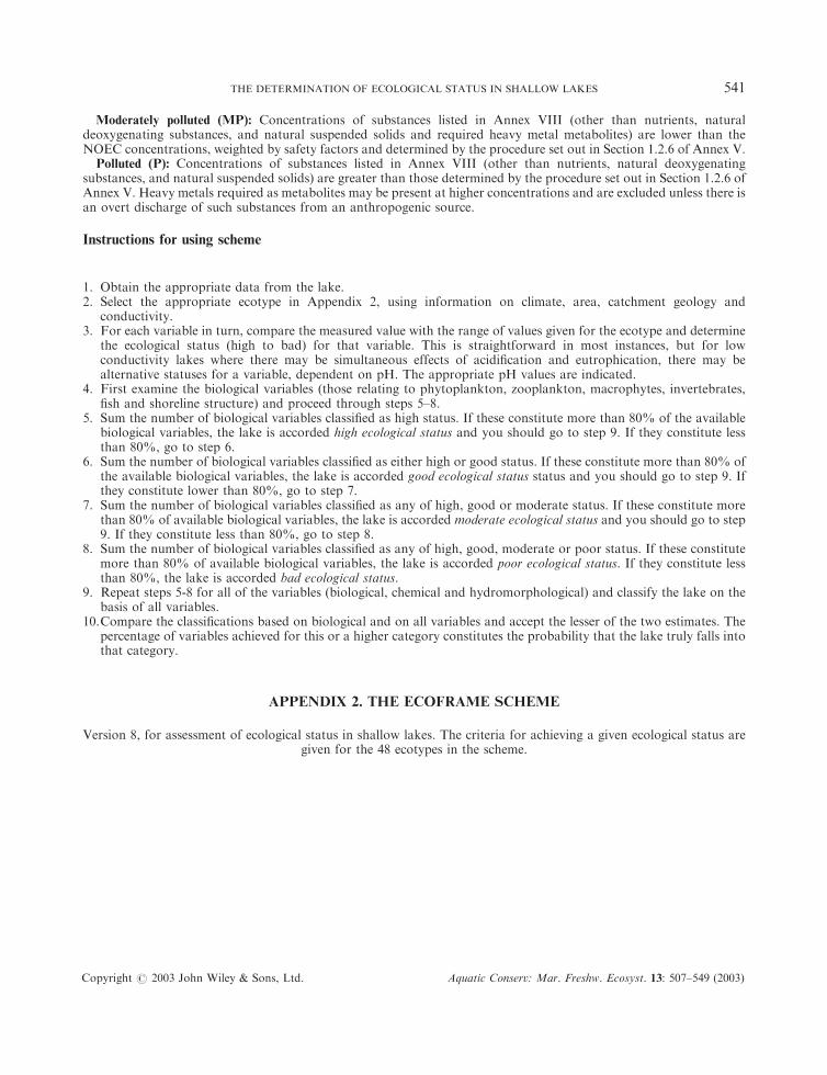
Moderately polluted (MP): Concentrations of substances listed in Annex VIII (other than nutrients, naturaldeoxygenating substances, and natural suspended solids and required heavy metal metabolites) are lower than theNOEC concentrations, weighted by safety factors and determined by the procedure set out in Section 1.2.6 of Annex V.Polluted (P): Concentrations of substances listed in Annex VIII (other than nutrients, natural deoxygenating

substances, and natural suspended solids) are greater than those determined by the procedure set out in Section 1.2.6 ofAnnex V. Heavy metals required as metabolites may be present at higher concentrations and are excluded unless there isan overt discharge of such substances from an anthropogenic source.

Instructions for using scheme

1. Obtain the appropriate data from the lake.2. Select the appropriate ecotype in Appendix 2, using information on climate, area, catchment geology and

conductivity.3. For each variable in turn, compare the measured value with the range of values given for the ecotype and determine

the ecological status (high to bad) for that variable. This is straightforward in most instances, but for lowconductivity lakes where there may be simultaneous effects of acidification and eutrophication, there may bealternative statuses for a variable, dependent on pH. The appropriate pH values are indicated.

4. First examine the biological variables (those relating to phytoplankton, zooplankton, macrophytes, invertebrates,fish and shoreline structure) and proceed through steps 5–8.

5. Sum the number of biological variables classified as high status. If these constitute more than 80% of the availablebiological variables, the lake is accorded high ecological status and you should go to step 9. If they constitute lessthan 80%, go to step 6.

6. Sum the number of biological variables classified as either high or good status. If these constitute more than 80% ofthe available biological variables, the lake is accorded good ecological status status and you should go to step 9. Ifthey constitute lower than 80%, go to step 7.

7. Sum the number of biological variables classified as any of high, good or moderate status. If these constitute morethan 80% of available biological variables, the lake is accorded moderate ecological status and you should go to step9. If they constitute less than 80%, go to step 8.

8. Sum the number of biological variables classified as any of high, good, moderate or poor status. If these constitutemore than 80% of available biological variables, the lake is accorded poor ecological status. If they constitute lessthan 80%, the lake is accorded bad ecological status.

9. Repeat steps 5-8 for all of the variables (biological, chemical and hydromorphological) and classify the lake on thebasis of all variables.

10.Compare the classifications based on biological and on all variables and accept the lesser of the two estimates. Thepercentage of variables achieved for this or a higher category constitutes the probability that the lake truly falls intothat category.

APPENDIX 2. THE ECOFRAME SCHEME

Version 8, for assessment of ecological status in shallow lakes. The criteria for achieving a given ecological status aregiven for the 48 ecotypes in the scheme.



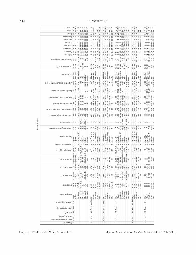
Sm

all c

old

lake

s

1<

10>

2<

100

Roc

k<

100

Hig

h5.

5-8

<15

(pH

>5.

5)<

0.3

>3(

pH>

5.5)

<10

(pH

>5.

5)A

Alg

or

Iso

>10

2>

0.5

>70

>30

>30

>30

<0.

25P

i + A

bex

5 to

10

>1

NN

NU

UI

UU

UU

Goo

d5.

5-8

16-3

0>

0.3<

0.4

>3(

pH>

5.5)

11 to

20

AA

lg o

r Is

o>

102

>0.

5>

70>

20<

30>

20<

3020

-30

>0.

25<

0.5

Pi +

Abe

x5

to 1

0>

1N

NN

DD

DD

MD

MC

MP

Mod

erat

e5.

5-8

31-5

0>

0.4<

0.5

2-2.

921

-30

AE

lpo

or C

anN

Y<

10>

33

0.2-

0.5

30-6

9>

10<

20>

10<

2010

to 2

0>

0.5<

1P

i or

Abe

x10

to 2

00.

5-1.

0M

MM

DD

DD

DC

P

Poo

r (a

cid)

>4.

5<5.

5<

15(p

H<

5.4)

>0.

5>

3(pH

<5.

4)<

10(p

H<

5.4)

AS

phag

<3>

0>

2 (S

ph)

<0.

2<

30>

5<10

>5<

10<

10<

0.25

Altd

<5

<0.

5S

MS

MS

MS

DS

DH

DS

DS

DS

CP

Poo

r (e

utr)

>8.

151

-75

>0.

51.

0-1.

931

-50

AIn

dist

inct

<3>

01

<0.

2<

30>

5<10

>5<

10<

10>

1A

ltd<

5 or

>20

<0.

5S

MS

MS

MS

DS

DH

DS

DS

DS

CP

Bad

(ac

id)

<4.

4<

5(pH

<5.

4)>

0.5

>3(

pH<

5.4)

<5

(pH

<5.

4)A

Sph

ag<

3>0

>2(

Sph

)<

0.2

<30

<5

<5

<10

No

anim

als

Abs

ent

0na

SM

SM

SM

SD

SD

SD

SD

SD

SC

PB

ad (

eutr

)>

8.1

>76

>0.

5<

0.9

>51

BA

bsen

tO

0<

0.2

<30

<5

<5

<10

No

anim

als

Altd

<5

<0.

5S

MS

MS

MS

DS

DS

DS

DS

DS

CP

2<

10>

2<

100

Roc

k10

1-80

0H

igh

6.0-

9.0

<30

<0.

6>

3<

10A

Alg

, Cha

r or

Iso

>10

2>

0.5

>70

>30

>30

>30

<0.

25P

i + A

bex

5 to

20

>1

NN

NN

NN

UU

IU

UU

UG

ood

6.0-

9.0

31-5

0>

0.6<

1.0

>3

11 to

20

AA

lg, C

har

or Is

o>

102

>0.

5>

70>

20<

30>

20<

3020

-30

>0.

25<

0.5

Pi +

Abe

x5

to 2

0>

1D

DD

DM

DM

CM

PM

oder

ate

6.0-

9.0

51-1

00>

1.0<

2.0

2-2.

921

-30

AE

lPo

or C

anN

y<

10>

33

0.2-

0.5

30-6

9>

10<

20>

10<

2010

to 2

0>

0.5<

1P

i or

Abe

x>

200.

5-1.

0M

MM

DD

DD

DC

PP

oor

<5.

9 or

>9.

110

1-15

0>

2.0

1.0-

1.9

31-5

0A

Indi

stin

ct<

3>0

1<

0.2

<30

>5<

10>

5<10

<10

>1

Altd

>20

<0.

5S

MS

MS

MS

DS

DH

DS

DS

DS

CP

Bad

<5.

9 or

>9.

1>

150

>2.

0<

0.9

>51

BA

bsen

tO

0<

0.2

<30

<5

<5

<10

No

anim

als

Altd

<5

<0.

5S

MS

MS

MS

DS

DS

DS

DS

DS

CP

3<

10>

2<

100

Roc

k>

801

Hig

h6.

0-9

<30

<0.

6>

3<

10A

Alg

or

Cha

r>

102

>0.

5>

70>

30>

30>

30<

0.25

Pi +

Abe

x5

to 2

0>

1N

NN

NN

NU

UI

UU

UU

Goo

d6.

0-9

31-5

0>

0.6<

1.0

>3

11 to

20

AA

lg o

r C

har

>10

2>

0.5

>70

>20

<30

>20

<30

20-3

0>

0.25

<0.

5P

i + A

bex

5 to

20

>1

DD

DD

MD

MC

MP

Mod

erat

e6.

0-9

51-1

00>

1.0<

2.0

2-2.

921

-30

AE

lpo

or C

anN

y<

10>

33

0.2-

0.5

30-6

9>

10<

20>

10<

2010

to 2

0>

0.5<

1P

i or

Abe

x>

200.

5-1.

0M

MM

DD

DD

DC

PP

oor

<5.

9 or

>9.

1>

101

>2.

01.

0-1.

931

-50

AIn

dist

inct

<3>

01

<0.

2<

30>

5<10

>5<

10<

10>

1A

ltd>

20<

0.5

SM

SM

SM

SD

SD

HD

SD

SD

SC

PB

ad<

5.9

or >

9.1

>15

0>

2.0

<0.

9>

51B

Abs

ent

O0

<0.

2<

30<

5<

5<

10N

o an

imal

sA

ltd<

5<

0.5

SM

SM

SM

SD

SD

SD

SD

SD

SC

P

4<

10>

2<

100

Pea

t<

100

Hig

h4.

0-8.

0<

15(p

H>

4)<

0.5

>2(

pH>

4)<

10(p

H>

5.5)

AA

lg o

r Is

o>

72

>0.

5>

70>

30>

30>

30<

0.25

Pi +

Abe

x5

to 1

0>

1N

NN

NN

NU

UI

UU

UU

Goo

d4.

0-8.

016

-30

>0.

5<1.

0>

2(pH

>4)

11 to

20

AA

lg o

r Is

o>

72

>0.

5>

70>

20<

30>

20<

3020

-30

>0.

25<

0.5

Pi +

Abe

x5

to 1

0>

1D

DD

DM

DM

CM

PM

oder

ate

4.0-

8.0

31-5

0>

1.0<

1.5

1.0-

1.9

21-3

0A

Elp

o or

Can

NY

<7>

33

0.2-

0.5

30-6

9>

10<

20>

10<

2010

to 2

0>

0.5<

1P

i or

Abe

x10

to 2

00.

5-1.

0M

MM

DD

DD

DC

PP

oor

(aci

d)<

3.9

<15

(pH

<3.

9)>

1.5

>2(

pH<

3.9)

<10

(pH

<5.

4)A

Sph

ag<

3>0

>2

(Sph

)<

0.2

<30

>5<

10>

5<10

<10

<0.

25A

ltd<

5<

0.5

SM

SM

SM

SM

SD

HD

SD

SD

SC

PP

oor

(eut

r)>

8.1

51-7

5>

1.5

1.0-

1.9

31-5

0A

Indi

stin

ct<

3>0

1<

0.2

<30

>5<

10>

5<10

<10

>1

Altd

<5

or >

20<

0.5

SM

SM

SM

SD

SD

HD

SD

SD

SC

PB

ad (

acid

)<

3.9

<5(

pH<

3.9)

>1.

5>

2(pH

<3.

9)<

5 (p

H<

5.4)

AS

phag

<3>

0>

2 (S

ph)

<0.

2<

30<

5<

5<

10N

o an

imal

sA

bsen

t0

naS

MS

MS

MS

DS

DS

DS

DS

DS

CP

Bad

(eu

tr)

>8.

1>

76>

1.5

<0.

9>

51B

Abs

ent

O0

<0.

2<

30<

5<

5<

10N

o an

imal

sA

ltd<

5<

0.5

SM

SM

SM

SD

SD

SD

SD

SD

SC

P

5<

10>

2<

100

Pea

t10

1-80

0H

igh

5.5-

9.0

<30

<0.

5>

2<

10A

Alg

, Cha

r or

Iso

>7

2>

0.5

>70

>30

>30

>30

<0.

25P

i + A

bex

5 to

20

>1

NN

NN

NN

UU

NN

NN

NN

U

IU

UU

U

UU

U

Goo

d5.

5-9.

031

-50

>0.

5<1.

0>

211

to 2

0A

Alg

, Cha

r or

Iso

>7

2>

0.5

>70

>20

<30

>20

<30

20-3

0>

0.25

<0.

5P

i + A

bex

5 to

20

>1

DD

DD

MD

MC

MP

Mod

erat

e5.

5-9.

051

-100

>1.

0<1.

51.

0-1.

921

-30

AE

lPo

or C

anN

y<

7>3

3>

0.2

30-6

9>

10<

20>

10<

2010

to 2

0>

0.5<

1P

i or

Abe

x>

200.

5-1.

0M

MM

DD

DD

DC

PP

oor

<5.

4 or

>9.

110

1-15

0>

1.5

0.5-

0.9

31-5

0A

Indi

stin

ct<

3>0

1<

0.2

<30

>5<

10>

5<10

<10

>1

Altd

>20

<0.

5S

MS

MS

MS

DS

DH

DS

DS

DS

CP

Bad

<5.

4 or

>9.

1>

150

>1.

5<

0.5

>51

BA

bsen

tO

0<

0.2

<30

<5

<5

<10

No

anim

als

Altd

<5

<0.

5S

MS

MS

MS

DS

DS

DS

DS

DS

CP

6<

10>

2<

100

Pea

t>

801

Hig

h6.

0-9

<30

<0.

5>

2<

10A

Alg

or

Cha

r>

72

>0.

5>

70>

30>

30>

30<

0.25

Pi +

Abe

x5

to 2

0>

1U

IU

Goo

d6.

0-9

31-5

0>

0.5<

1.0

>2

11 to

20

AA

lg o

r C

har

>7

2>

0.5

>70

>20

<30

>20

<30

20-3

0>

0.25

<0.

5P

i + A

bex

5 to

20

>1

DD

DD

MD

MC

MP

Mod

erat

e6.

0-9

51-1

00>

1.0<

1.5

1.0-

1.9

21-3

0A

Elp

o or

Can

Ny

<7>

33

>0.

230

-69

>10

<20

>10

<20

10 to

20

>0.

5<1

Pi o

r A

bex

>20

0.5-

1.0

MM

MD

DD

DD

CP

Poo

r<

5.9

or >

9.1

101-

150

>1.

50.

5-0.

931

-50

AIn

dist

inct

<3>

01

<0.

2<

30>

5<10

>5<

10<

10>

1A

ltd>

20<

0.5

SM

SM

SM

SD

SD

HD

SD

SD

SC

PB

ad<

5.9

or >

9.1

>15

0>

1.5

<0.

5>

51B

Abs

ent

O0

<0.

2<

30<

5<

5<

10N

o an

imal

sA

ltd<

5<

0.5

SM

SM

SM

SD

SD

SD

SD

SD

SC

P

Groundwater

Oxygen

Salinity

Pollution

Depth var.n

Substrate

Lake shore

Temperature



Water flow

Residence



Oligo: chiro [soft substr] (ratio by no.)

Fish community

Plant abundance

Cladocera (no. large : total no.)

Zoopl:phytopl (mg:µg chlorophyll a)




Plant community

Plant diversity (species number)

pH (log units)

Total P (µg L-1)

Total N (mg L-1)

Secchi depth (m)

Temp. of warmest month (°C)

Ice cover (months)

Ecotype no.

Ecological status

Area (km2)

Catchment geology


B. MOSS ET AL.542


Sm

all c

ool l

akes

7>

10>

2<

100

Roc

k<

100

Hig

h5.

5-8

<15

(pH

>5.

5)<

0.3

>3(

pH>

5.5)

<10

(pH

>5.

5)A

Iso

>10

2>

0.5

>70

>20

>30

>30

<0.

25P

i + A

bex

5 to

10

>1

NN

NN

NN

UU

NN

NN

NN

U

IU

UU

UG

ood

5.5-

816

-30

>0.

3<0.

4>

3(pH

>5.

5)11

to 2

0A

Iso

>10

2>

0.5

>70

>15

<20

>20

<30

20-3

0>

0.25

<0.

5P

i + A

bex

5 to

10

>1

DD

DD

MD

MC

MP

Mod

erat

e5.

5-8

31-5

0>

0.4<

0.5

2-2.

921

-30

AE

lPo

or C

anN

ym<

10>

33

0.2-

0.5

30-6

9>

10<

15>

10<

2010

to 2

0>

0.5<

1P

i or

Abe

x10

to 2

00.

5-1.

0M

MM

DD

DD

DC

PP

oor

(aci

d)>

4.5<

5.5

<15

(pH

<5.

4)>

0.5

>3(

pH<

5.4)

<10

(pH

<5.

4)A

Sph

ag<

3>0

>2

(Sph

)<

0.2

<30

>5<

10>

5<10

<10

<0.

25A

ltd<

5<

0.5

SM

SM

SM

SD

SD

HD

SD

SD

SC

PP

oor

(eut

r)>

8.1

51-7

5>

0.5

1.0-

1.9

31-5

0B

Indi

stin

ct<

3>0

1<

0.2

<30

>5<

10>

5<10

<10

>1

Altd

<5

or >

20<

0.5

SM

SM

SM

SD

SD

HD

SD

SD

SC

PB

ad (

acid

)<

4.4

<5(

pH<

5.4)

>0.

5>

3(pH

<5.

4)<

5 (p

H<

5.4)

AS

phag

<3>

0>

2(S

ph)

<0.

2<

30<

5<

5<

10N

o an

imal

sA

bsen

t0

naS

MS

MS

MS

DS

DS

DS

DS

DS

CP

Bad

(eu

tr)

>8.

1>

76>

0.5

<0.

9>

51C

Abs

ent

O0

<0.

2<

30<

5<

5<

10N

o an

imal

sA

ltd<

5<

0.5

SM

SM

SM

SD

SD

SD

SD

SD

SC

P

8>

10>

2<

100

Roc

k10

1-80

0H

igh

6.0-

9.0

<30

<0.

6>

3<

10A

Iso

or C

har

>10

2>

0.5

>70

>20

>30

>30

<0.

25P

i + A

bex

5 to

20

>1

UI

UU

UU

Goo

d6.

0-9.

031

-50

>0.

6<1.

0>

311

to 2

0A

Iso

or C

har

>10

2>

0.5

>70

>15

<20

>20

<30

20-3

0>

0.25

<0.

5P

i + A

bex

5 to

20

>1

DD

DD

MD

MC

MP

Mod

erat

e6.

0-9.

051

-100

>1.

0<2.

02-

2.9

21-3

0A

ElP

o or

Can

Nym

<10

>3

30.

2-0.

530

-69

>10

<15

>10

<20

10 to

20

>0.

5<1

Pi o

r A

bex

>20

0.5-

1.0

MM

MD

DD

DD

CP

Poo

r<

5.9

or >

9.1

101-

150

>2.

01.

0-1.

931

-50

BIn

dist

inct

<3>

01

<0.

2<

30>

5<10

>5<

10<

10>

1A

ltd>

20<

0.5

SM

SM

SM

SD

SD

HD

SD

SD

SC

PB

ad<

5.9

or >

9.1

>15

0>

2.0

<0.

9>

51C

Abs

ent

O0

<0.

2<

30<

5<

5<

10N

o an

imal

sA

ltd<

5<

0.5

SM

SM

SM

SD

SD

SD

SD

SD

SC

P

9>

10>

2<

100

Roc

k>

801

Hig

h6.

0-9

<30

<0.

6>

3<

10A

Cha

r>

102

>0.

5>

70>

20>

30>

30<

0.25

Pi +

Abe

x5

to 2

0>

1N

NN

NN

NU

U

NN

NN

NN

U

NN

NN

NN

U

NN

NN

NN

U

IU

UU

UG

ood

6.0-

931

-50

>0.

6<1.

0>

311

to 2

0A

Cha

r>

102

>0.

5>

70>

15<

20>

20<

3020

-30

>0.

25<

0.5

Pi +

Abe

x5

to 2

0>

1D

DD

DM

DM

CM

PM

oder

ate

6.0-

951

-100

>1.

0<2.

02-

2.9

21-3

0A

Elp

o or

Can

Nym

<10

>3

30.

2-0.

530

-69

>10

<15

>10

<20

10 to

20

>0.

5<1

Pi o

r A

bex

>20

0.5-

1.0

MM

MD

DD

DD

CP

Poo

r<

5.9

or >

9.1

>10

1>

2.0

1.0-

1.9

31-5

0B

Indi

stin

ct<

3>0

1<

0.2

<30

>5<

10>

5<10

<10

>1

Altd

>20

<0.

5S

MS

MS

MS

DS

DH

DS

DS

DS

CP

Bad

<5.

9 or

>9.

1>

150

>2.

0<

0.9

>51

CA

bsen

tO

0<

0.2

<30

<5

<5

<10

No

anim

als

Altd

<5

<0.

5S

MS

MS

MS

DS

DS

DS

DS

DS

CP

10>

10>

2<

100

Pea

t<

100

Hig

h4.

0-8.

0<

15(p

H>

4)<

0.5

>2(

pH>

4)<

10(p

H>

5.5)

AIs

o>

72

>0.

5>

70>

20>

30>

30<

0.25

Pi +

Abe

x5

to 1

0>

1U

IU

UU

UG

ood

4.0-

8.0

16-3

0>

0.5<

1.0

>2(

pH>

4)11

to 2

0A

Iso

>7

2>

0.5

>70

>15

<20

>20

<30

20-3

0>

0.25

<0.

5P

i + A

bex

5 to

10

>1

DD

DD

MD

MC

MP

Mod

erat

e4.

0-8.

031

-50

>1.

0<1.

51.

0-1.

921

-30

AE

lPo

or C

anN

Ym

<7>

33

0.2-

0.5

30-6

9>

10<

15>

10<

2010

to 2

0>

0.5<

1P

i or

Abe

x10

to 2

00.

5-1.

0M

MM

DD

DD

DC

PP

oor

(aci

d)<

3.9

<15

(pH

<3.

9)>

1.5

>2(

pH<

3.9)

<10

(pH

<5.

4)A

Sph

ag<

3>0

>2

(Sph

)<

0.2

<30

>5<

10>

5<10

<10

<0.

25A

ltd<

5<

0.5

SM

SM

SM

SM

SD

HD

SD

SD

SC

PP

oor(

eutr

)>

8.1

51-7

5>

1.5

1.0-

1.9

31-5

0B

Indi

stin

ct<

3>0

1<

0.2

<30

>5<

10>

5<10

<10

>1

Altd

<5

or >

20<

0.5

SM

SM

SM

SD

SD

HD

SD

SD

SC

PB

ad (

acid

)<

3.9

<5(

pH<

3.9)

>1.

5>

2(pH

<3.

9)<

5 (p

H<

5.4)

AS

phag

<3>

0>

2 (S

ph)

<0.

2<

30<

5<

5<

10N

o an

imal

sA

bsen

t0

naS

MS

MS

MS

DS

DS

DS

DS

DS

CP

Bad

(eu

tr)

>8.

1>

76>

1.5

<0.

9>

51C

Abs

ent

O0

<0.

2<

30<

5<

5<

10N

o an

imal

sA

ltd<

5<

0.5

SM

SM

SM

SD

SD

SD

SD

SD

SC

P

11>

10>

2<

100

Pea

t10

1-80

0H

igh

5.5-

9.0

<30

<0.

5>

2<

10A

Iso

or C

har

>7

2>

0.5

>70

>20

>30

>30

<0.

25P

i + A

bex

5 to

20

>1

UI

UU

UU

Goo

d5.

5-9.

031

-50

>0.

5<1.

0>

211

to 2

0A

Iso

or C

har

>7

2>

0.5

>70

>15

<20

>20

<30

20-3

0>

0.25

<0.

5P

i + A

bex

5 to

20

>1

DD

DD

MD

MC

MP

Mod

erat

e5.

5-9.

051

-100

>1.

0<1.

51.

0-1.

921

-30

AE

lPo

or C

anN

ym<

7>3

3>

0.2

30-6

9>

10<

15>

10<

2010

to 2

0>

0.5<

1P

i or

Abe

x>

200.

5-1.

0M

MM

DD

DD

DC

PP

oor

<5.

4 or

>9.

110

1-15

0>

1.5

0.5-

0.9

31-5

0B

Indi

stin

ct<

3>0

1<

0.2

<30

>5<

10>

5<10

<10

>1

Altd

>20

<0.

5S

MS

MS

MS

DS

DH

DS

DS

DS

CP

Bad

<5.

4 or

>9.

1>

150

>1.

5<

0.5

>51

CA

bsen

tO

0<

0.2

<30

<5

<5

<10

No

anim

als

Altd

<5

<0.

5S

MS

MS

MS

DS

DS

DS

DS

DS

CP

12>

10>

2<

100

Pea

t>

801

Hig

h6.

0-9

<30

<0.

5>

2<

10A

Cha

r>

72

>0.

5>

70>

20>

30>

30<

0.25

Pi +

Abe

x5

to 2

0>

1U

IU

UU

UG

ood

6.0-

931

-50

>0.

5<1.

0>

211

to 2

0A

Cha

r>

72

>0.

5>

70>

15<

20>

20<

3020

-30

>0.

25<

0.5

Pi +

Abe

x5

to 2

0>

1D

DD

DM

DM

CM

PM

oder

ate

6.0-

951

-100

>1.

0<1.

51.

0-1.

921

-30

AE

lpo

or C

anN

ym<

7>3

3>

0.2

30-6

9>

10<

15>

10<

2010

to 2

0>

0.5<

1P

i or

Abe

x>

200.

5-1.

0M

MM

DD

DD

DC

PP

oor

<5.

9 or

>9.

110

1-15

0>

1.5

0.5-

0.9

31-5

0B

Indi

stin

ct<

3>0

1<

0.2

<30

>5<

10>

5<10

<10

>1

Altd

>20

<0.

5S

MS

MS

MS

DS

DH

DS

DS

DS

CP

Bad

<5.

9 or

>9.

1>

150

>1.

5<

0.5

>51

CA

bsen

tO

0<

0.2

<30

<5

<5

<10

No

anim

als

Altd

<5

<0.

5S

MS

MS

MS

DS

DS

DS

DS

DS

CP

Oxygen

Salinity

Pollution

Ecotype no.

Depth var.n

Substrate

Lake shore

Temperature


Water flow


Residence

Groundwater



Fish community


Plant abundance






Plant community


pH (log units)

Total P (µg L-1)

Total N (mg L-1)

Secchi depth (m)


Ice cover (months)

Ecological status

Area (km2)

Catchment geology




Sm

all t

empe

rate

lake

s

13>

10<

25<

2<

100

Roc

k<

100

Hig

h5.

5-8

<15

(pH

>5.

5)<

0.3

>3(

pH>

5.5)

<10

(pH

>5.

5)A

Iso

>10

2>

0.5

>70

>20

>30

>20

<0.

25P

i + A

bex

5 to

10

>1

NN

NN

NN

UI

UU

UU

Goo

d5.

5-8

16-3

0>

0.3<

0.4

>3(

pH>

5.5)

11 to

20

AIs

o>

102

>0.

5>

70>

15<

20>

20<

30>

20>

0.25

<0.

5P

i + A

bex

5 to

10

>1

DU D

DD

MD

MC

MP

Mod

erat

e5.

5-8

31-5

0>

0.4<

0.5

2-2.

921

-30

AE

lPo

or C

anN

ym<

10>

33

0.2-

0.5

30-6

9>

10<

15>

10<

2010

to 2

0>

0.5<

1P

i or

Abe

x10

to 2

00.

5-1.

0M

MM

DD

DD

DC

PP

oor(

acid

)>

4.5<

5.5

<15

(pH

<5.

4)>

0.5

>3(

pH<

5.4)

<10

(pH

<5.

4)A

Sph

ag<

3>0

>2

(Sph

)<

0.2

<30

>5<

10>

5<10

<10

<0.

25A

ltd<

5<

0.5

SM

SM

SM

SD

SD

HD

SD

SD

SC

PP

oor

(eut

r)>

8.1

51-7

5>

0.5

1.0-

1.9

31-5

0B

Indi

stin

ct<

3>0

1<

0.2

<30

>5<

10>

5<10

<10

>1

Altd

<5

or >

20<

0.5

SM

SM

SM

SD

SD

HD

SD

SD

SC

PB

ad (

acid

)<

4.4

<5(

pH<

5.4)

>0.

5>

3(pH

<5.

4)<

5 (p

H<

5.4)

AS

phag

<3>

0>

2(S

ph)

<0.

2<

30<

5<

5<

10N

o an

imal

sA

bsen

t0

naS

MS

MS

MS

DS

DS

DS

DS

DS

CP

Bad

(eu

tr)

>8.

1>

76>

0.5

<0.

9>

51C

Abs

ent

O0

<0.

2<

30<

5<

5<

10N

o an

imal

sA

ltd<

5<

0.5

SM

SM

SM

SD

SD

SD

SD

SD

SC

P

14>

10<

25<

2<

100

Roc

k10

1-80

0H

igh

6.0-

9.0

<30

<0.

6>

3<

10A

Iso

or C

har

>10

2>

0.5

>70

>20

>30

>20

<0.

25P

i + A

bex

5 to

20

>1

UI

UG

ood

6.0-

9.0

31-5

0>

0.6<

1.0

>3

11 to

20

AIs

o or

Cha

r>

102

>0.

5>

70>

15<

20>

20<

30>

20>

0.25

<0.

5P

i + A

bex

5 to

20

>1

DD

DM

DM

CM

PM

oder

ate

6.0-

9.0

51-1

00>

1.0<

2.0

2-2.

921

-30

AE

lPo

or C

anN

ym<

10>

33

0.2-

0.5

30-6

9>

10<

15>

10<

2010

to 2

0>

0.5<

1P

i or

Abe

x>

200.

5-1.

0M

MM

DD

DD

DC

PP

oor

<5.

9 or

>9.

110

1-15

0>

2.0

1.0-

1.9

31-5

0B

Indi

stin

ct<

3>0

1<

0.2

<30

>5<

10>

5<10

<10

>1

Altd

>20

<0.

5S

MS

MS

MS

DS

DH

DS

DS

DS

CP

Bad

<5.

9 or

>9.

1>

150

>2.

0<

0.9

>51

CA

bsen

tO

0<

0.2

<30

<5

<5

<10

No

anim

als

Altd

<5

<0.

5S

MS

MS

MS

DS

DS

DS

DS

DS

CP

15>

10<

25<

2<

100

Roc

k>

801

Hig

h6.

0-9

<30

<0.

6>

3<

10A

Cha

r>

102

>0.

5>

70>

20>

30>

20<

0.25

Pi +

Abe

x5

to 2

0>

1U

IU

Goo

d6.

0-9

31-5

0>

0.6<

1.0

>3

11 to

20

AC

har

>10

2>

0.5

>70

>15

<20

>20

<30

>20

>0.

25<

0.5

Pi +

Abe

x5

to 2

0>

1D

DD

MD

MC

MP

Mod

erat

e6.

0-9

51-1

00>

1.0<

2.0

2-2.

921

-30

AE

lpo

or C

anN

ym<

10>

33

0.2-

0.5

30-6

9>

10<

15>

10<

2010

to 2

0>

0.5<

1P

i or

Abe

x>

200.

5-1.

0M

MM

DD

DD

DC

PP

oor

<5.

9 or

>9.

1>

101

>2.

01.

0-1.

931

-50

BIn

dist

inct

<3>

01

<0.

2<

30>

5<10

>5<

10<

10>

1A

ltd>

20<

0.5

SM

SM

SM

SD

SD

HD

SD

SD

SC

PB

ad<

5.9

or >

9.1

>15

0>

2.0

<0.

9>

51C

Abs

ent

O0

<0.

2<

30<

5<

5<

10N

o an

imal

sA

ltd<

5<

0.5

SM

SM

SM

SD

SD

SD

SD

SD

SC

P

16>

10<

25<

2<

100

Pea

t<

100

Hig

h4.

0-8.

0<

15(p

H>

4)<

0.5

>2(

pH>

4)<

10(p

H>

5.5)

AIs

o>

72

>0.

5>

70>

20>

30>

20<

0.25

Pi +

Abe

x5

to 1

0>

1U

IU

Goo

d4.

0-8.

016

-30

>0.

5<1.

0>

2(pH

>4)

11 to

20

AIs

o>

72

>0.

5>

70>

15<

20>

20<

30>

20>

0.25

<0.

5P

i + A

bex

5 to

10

>1

DD

DM

DM

CM

PM

oder

ate

4.0-

8.0

31-5

0>

1.0<

1.5

1.0-

1.9

21-3

0A

ElP

o or

Can

NY

m<

7>3

30.

2-0.

530

-69

>10

<15

>10

<20

10 to

20

>0.

5<1

Pi o

r A

bex

10 to

20

0.5-

1.0

MM

MD

DD

DD

CP

Poo

r (a

cid)

<3.

9<

15(p

H<

3.9)

>1.

5>

2(pH

<3.

9)<

10(p

H<

5.4)

AS

phag

<3>

0>

2 (S

ph)

<0.

2<

30>

5<10

>5<

10<

10<

0.25

Altd

<5

<0.

5S

MS

MS

MS

MS

DH

DS

DS

DS

CP

Poo

r (e

utr)

>8.

151

-75

>1.

51.

0-1.

931

-50

BIn

dist

inct

<3>

01

<0.

2<

30>

5<10

>5<

10<

10>

1A

ltd<

5 or

>20

<0.

5S

MS

MS

MS

DS

DH

DS

DS

DS

CP

Bad

(ac

id)

<3.

9<

5(pH

<3.

9)>

1.5

>2(

pH<

3.9)

<5

(pH

<5.

4)A

Sph

ag<

3>0

>2

(Sph

)<

0.2

<30

<5

<5

<10

No

anim

als

Abs

ent

0na

SM

SM

SM

SD

SD

SD

SD

SD

SC

PB

ad (

eutr

)>

8.1

>76

>1.

5<

0.9

>51

CA

bsen

tO

0<

0.2

<30

<5

<5

<10

No

anim

als

Altd

<5

<0.

5S

MS

MS

MS

DS

DS

DS

DS

DS

CP

17>

10<

25<

2<

100

Pea

t10

1-80

0H

igh

5.5-

9.0

<30

<0.

5>

2<

10A

Iso

or C

har

>7

2>

0.5

>70

>20

>30

>20

<0.

25P

i + A

bex

5 to

20

>1

UI

UG

ood

5.5-

9.0

31-5

0>

0.5<

1.0

>2

11 to

20

AIs

o or

Cha

r>

72

>0.

5>

70>

15<

20>

20<

30>

20>

0.25

<0.

5P

i + A

bex

5 to

20

>1

DD

DM

DM

CM

PM

oder

ate

5.5-

9.0

51-1

00>

1.0<

1.5

1.0-

1.9

21-3

0A

ElP

o or

Can

Nym

<7>

33

>0.

230

-69

>10

<15

>10

<20

10 to

20

>0.

5<1

Pi o

r A

bex

>20

0.5-

1.0

MM

MD

DD

DD

CP

Poo

r<

5.4

or >

9.1

101-

150

>1.

50.

5-0.

931

-50

BIn

dist

inct

<3>

01

<0.

2<

30>

5<10

>5<

10<

10>

1A

ltd>

20<

0.5

SM

SM

SM

SD

SD

HD

SD

SD

SC

PB

ad<

5.4

or >

9.1

>15

0>

1.5

<0.

5>

51C

Abs

ent

O0

<0.

2<

30<

5<

5<

10N

o an

imal

sA

ltd<

5<

0.5

SM

SM

SM

SD

SD

SD

SD

SD

SC

P

18>

10<

25<

2<

100

Pea

t>

801

Hig

h6.

0-9

<30

<0.

5>

2<

10A

Cha

r>

72

>0.

5>

70>

20>

30>

20<

0.25

Pi +

Abe

x5

to 2

0>

1U

IU

Goo

d6.

0-9

31-5

0>

0.5<

1.0

>2

11 to

20

AC

har

>7

2>

0.5

>70

>15

<20

>20

<30

>20

>0.

25<

0.5

Pi +

Abe

x5

to 2

0>

1D

DD

MD

MC

MP

Mod

erat

e6.

0-9

51-1

00>

1.0<

1.5

1.0-

1.9

21-3

0A

Elp

o or

Can

Nym

<7>

33

>0.

230

-69

>10

<15

>10

<20

10 to

20

>0.

5<1

Pi o

r A

bex

>20

0.5-

1.0

MM

MD

DD

DD

CP

Poo

r<

5.9

or >

9.1

101-

150

>1.

50.

5-0.

931

-50

BIn

dist

inct

<3>

01

<0.

2<

30>

5<10

>5<

10<

10>

1A

ltd>

20<

0.5

SM

SM

SM

SD

SD

HD

SD

SD

SC

PB

ad<

5.9

or >

9.1

>15

0>

1.5

<0.

5>

51C

Abs

ent

O0

<0.

2<

30<

5<

5<

10N

o an

imal

sA

ltd<

5<

0.5

SM

SM

SM

SD

SD

SD

SD

SD

SC

P

Groundwater

Oxygen

Salinity

Pollution

Depth var.n

Substrate

Lake shore

Temperature



Water flow

Residence




Fish community

Plant abundance






Plant community


pH (log units)

Total P (µg L-1)

Total N (mg L-1)

Secchi depth (m)


Ice cover (months)

Ecotype no.

Ecological status

Area (km2)

Catchment geology


NN

NN

NN

UU

UU D

NN

NN

NN

UU

UU D

NN

NN

NN

UU

UU D

NN

NN

NN

UU

UU D

NN

NN

NN

UU

UU D

B. MOSS ET AL.544


Larg

e co

ld la

kes

25<

10>

2>

100

Roc

k<

100

Hig

h5.

5-8

<15

(pH

>5.

5)<

0.3

>3(

pH>

5.5)

<10

(pH

>5.

5)A

Alg

or

Iso

>10

2>

0.5

>70

>20

>30

>30

<0.

25P

i + A

bex

5 to

10

>1

NN

NU

UI

UU

UU

Goo

d5.

5-8

16-3

0>

0.3<

0.4

>3(

pH>

5.5)

11 to

20

AA

lg o

r Is

o>

102

>0.

5>

70>

15<

20>

20<

3020

-30

>0.

25<

0.5

Pi +

Abe

x5

to 1

0>

1N

NN

DD

DD

MD

MC

MP

Mod

erat

e5.

5-8

31-5

0>

0.4<

0.5

2-2.

921

-30

AE

lpo

or C

anN

Y<

10>

33

0.2-

0.5

30-6

9>

10<

15>

10<

2010

to 2

0>

0.5<

1P

i or

Abe

x10

to 2

00.

5-1.

0M

MM

DD

DD

DC

PP

oor

(aci

d)>

4.5<

5.5

<15

(pH

<5.

4)>

0.5

>3(

pH<

5.4)

<10

(pH

<5.

4)A

Sph

ag<

3>0

>2

(Sph

)<

0.2

<30

>5<

10>

5<10

<10

<0.

25A

ltd<

5<

0.5

SM

SM

SM

SD

SD

HD

SD

SD

SC

PP

oor

(eut

r)>

8.1

51-7

5>

0.5

1.0-

1.9

31-5

0B

Indi

stin

ct<

3>0

1<

0.2

<30

>5<

10>

5<10

<10

>1

Altd

<5

or >

20<

0.5

SM

SM

SM

SD

SD

HD

SD

SD

SC

PB

ad (

acid

)<

4.4

<5(

pH<

5.4)

>0.

5>

3(pH

<5.

4)<

5 (p

H<

5.4)

AS

phag

<3>

0>

2(S

ph)

<0.

2<

30<

5<

5<

10N

o an

imal

sA

bsen

t0

naS

MS

MS

MS

DS

DS

DS

DS

DS

CP

Bod

(eu

tro)

>8.

1>

76>

0.5

<0.

9>

51C

Abs

ent

O0

<0.

2<

30<

5<

5<

10N

o an

imal

sA

ltd<

5<

0.5

SM

SM

SM

SD

SD

SD

SD

SD

SC

P

26<

10>

2>

100

Roc

k10

1-80

0H

igh

6.0-

9.0

<30

<0.

6>

3<

10A

Alg

, Cha

r or

Iso

>10

2>

0.5

>70

>20

>30

>30

<0.

25P

i + A

bex

5 to

20

>1

NN

NU

UI

UU

UU

Goo

d6.

0-9.

031

-50

>0.

6<1.

0>

311

to 2

0A

Alg

, Cha

r or

Iso

>10

2>

0.5

>70

>15

<20

>20

<30

20-3

0>

0.25

<0.

5P

i + A

bex

5 to

20

>1

NN

ND

DD

DM

DM

CM

PM

oder

ate

6.0-

9.0

51-1

00>

1.0<

2.0

2-2.

921

-30

AE

lPo

or C

anN

y<

10>

33

0.2-

0.5

30-6

9>

10<

15>

10<

2010

to 2

0>

0.5<

1P

i or

Abe

x>

200.

5-1.

0M

MM

DD

DD

DC

PP

oor

<5.

9 or

>9.

110

1-15

0>

2.0

1.0-

1.9

31-5

0B

Indi

stin

ct<

3>0

1<

0.2

<30

>5<

10>

5<10

<10

>1

Altd

>20

<0.

5S

MS

MS

MS

DS

DH

DS

DS

DS

CP

Bad

<5.

9 or

>9.

1>

150

>2.

0<

0.9

>51

CA

bsen

tO

0<

0.2

<30

<5

<5

<10

No

anim

als

Altd

<5

<0.

5S

MS

MS

MS

DS

DS

DS

DS

DS

CP

27<

10>

2>

100

Roc

k>

801

Hig

h6.

0-9

<30

<0.

6>

3<

10A

Alg

or

Cha

r>

102

>0.

5>

70>

20>

30>

30<

0.25

Pi +

Abe

x5

to 2

0>

1N

NN

UU

NN

NU

NN

NU

IU

UU

U

UU

U

UU

U

NN

NU

UU

U

Goo

d6.

0-9

31-5

0>

0.6<

1.0

>3

11 to

20

AA

lg o

r C

har

>10

2>

0.5

>70

>15

<20

>20

<30

20-3

0>

0.25

<0.

5P

i + A

bex

5 to

20

>1

NN

ND

D

NN

ND

NN

ND

NN

ND

DD

MD

MC

MP

Mod

erat

e6.

0-9

51-1

00>

1.0<

2.0

2-2.

921

-30

AE

lpo

or C

anN

y<

10>

33

0.2-

0.5

30-6

9>

10<

15>

10<

2010

to 2

0>

0.5<

1P

i or

Abe

x>

200.

5-1.

0M

MM

DD

DD

DC

PP

oor

<5.

9 or

>9.

1>

101

>2.

01.

0-1.

931

-50

BIn

dist

inct

<3>

01

<0.

2<

30>

5<10

>5<

10<

10>

1A

ltd>

20<

0.5

SM

SM

SM

SD

SD

HD

SD

SD

SC

PB

ad<

5.9

or >

9.1

>15

0>

2.0

<0.

9>

51C

Abs

ent

O0

<0.

2<

30<

5<

5<

10N

o an

imal

sA

ltd<

5<

0.5

SM

SM

SM

SD

SD

SD

SD

SD

SC

P

28<

10>

2>

100

Pea

t<

100

Hig

h4.

0-8.

0<

15(p

H>

4)<

0.5

>2(

pH>

4)<

10(p

H>

5.5)

AA

lg o

r Is

o>

72

>0.

5>

70>

20>

30>

30<

0.25

Pi +

Abe

x5

to 1

0>

1U

IU

Goo

d4.

0-8.

016

-30

>0.

5<1.

0>

2(pH

>4)

11 to

20

AA

lg o

r Is

o>

72

>0.

5>

70>

15<

20>

20<

3020

-30

>0.

25<

0.5

Pi +

Abe

x5

to 1

0>

1D

DD

MD

MC

MP

Mod

erat

e4.

0-8.

031

-50

>1.

0<1.

51.

0-1.

921

-30

AE

lpo

or C

anN

Y<

7>3

30.

2-0.

530

-69

>10

<15

>10

<20

10 to

20

>0.

5<1

Pi o

r A

bex

10 to

20

0.5-

1.0

MM

MD

DD

DD

CP

Poo

r (a

cid)

<3.

9<

15(p

H<

3.9)

>1.

5>

2(pH

<3.

9)<

10(p

H<

5.4)

AS

phag

<3>

0>

2 (S

ph)

<0.

2<

30>

5<10

>5<

10<

10<

0.25

Altd

<5

<0.

5S

MS

MS

MS

MS

DH

DS

DS

DS

CP

Poo

r (e

utr)

>8.

151

-75

>1.

51.

0-1.

931

-50

BIn

dist

inct

<3>

01

<0.

2<

30>

5<10

>5<

10<

10>

1A

ltd<

5 or

>20

<0.

5S

MS

MS

MS

DS

DH

DS

DS

DS

CP

Bad

(ac

id)

<3.

9<

5(pH

<3.

9)>

1.5

>2(

pH<

3.9)

<5

(pH

<5.

4)A

Sph

ag<

3>0

>2

(Sph

)<

0.2

<30

<5

<5

<10

No

anim

als

Abs

ent

0na

SM

SM

SM

SD

SD

SD

SD

SD

SC

PB

ad (

eutr

)>

8.1

>76

>1.

5<

0.9

>51

CA

bsen

tO

0<

0.2

<30

<5

<5

<10

No

anim

als

Altd

<5

<0.

5S

MS

MS

MS

DS

DS

DS

DS

DS

CP

29<

10>

2>

100

Pea

t10

1-80

0H

igh

5.5-

9.0

<30

<0.

5>

2<

10A

Alg

, Cha

r or

Iso

>7

2>

0.5

>70

>20

>30

>30

<0.

25P

i + A

bex

5 to

20

>1

UI

UG

ood

5.5-

9.0

31-5

0>

0.5<

1.0

>2

11 to

20

AA

lg, C

har

or Is

o>

72

>0.

5>

70>

15<

20>

20<

3020

-30

>0.

25<

0.5

Pi +

Abe

x5

to 2

0>

1D

DD

MD

MC

MP

Mod

erat

e5.

5-9.

051

-100

>1.

0<1.

51.

0-1.

921

-30

AE

lPo

or C

anN

y<

7>3

3>

0.2

30-6

9>

10<

15>

10<

2010

to 2

0>

0.5<

1P

i or

Abe

x>

200.

5-1.

0M

MM

DD

DD

DC

PP

oor

<5.

4 or

>9.

110

1-15

0>

1.5

0.5-

0.9

31-5

0B

Indi

stin

ct<

3>0

1<

0.2

<30

>5<

10>

5<10

<10

>1

Altd

>20

<0.

5S

MS

MS

MS

DS

DH

DS

DS

DS

CP

Bad

<5.

4 or

>9.

1>

150

>1.

5<

0.5

>51

CA

bsen

tO

0<

0.2

<30

<5

<5

<10

No

anim

als

Altd

<5

<0.

5S

MS

MS

MS

DS

DS

DS

DS

DS

CP

30<

10>

2>

100

Pea

t>

801

Hig

h6.

0-9

<30

<0.

5>

2<

10A

Alg

or

Cha

r>

72

>0.

5>

70>

20>

30>

30<

0.25

Pi +

Abe

x5

to 2

0>

1U

IU

Goo

d6.

0-9

31-5

0>

0.5<

1.0

>2

11 to

20

AA

lg o

r C

har

>7

2>

0.5

>70

>15

<20

>20

<30

20-3

0>

0.25

<0.

5P

i + A

bex

5 to

20

>1

DD

DM

DM

CM

PM

oder

ate

6.0-

951

-100

>1.

0<1.

51.

0-1.

921

-30

AE

lpo

or C

anN

y<

7>3

3>

0.2

30-6

9>

10<

15>

10<

2010

to 2

0>

0.5<

1P

i or

Abe

x>

200.

5-1.

0M

MM

DD

DD

DC

PP

oor

<5.

9 or

>9.

110

1-15

0>

1.5

0.5-

0.9

31-5

0B

Indi

stin

ct<

3>0

1<

0.2

<30

>5<

10>

5<10

<10

>1

Altd

>20

<0.

5S

MS

MS

MS

DS

DH

DS

DS

DS

CP

Bad

<5.

9 or

>9.

1>

150

>1.

5<

0.5

>51

CA

bsen

tO

0<

0.2

<30

<5

<5

<10

No

anim

als

Altd

<5

<0.

5S

MS

MS

MS

DS

DS

DS

DS

DS

CP

Groundwater

Oxygen

Salinity

Pollution

Depth var.n

Substrate

Lake shore

Temperature



Water flow

Residence




Fish community

Plant abundance


Zoopl:phytopl (mg:)


Chlorophylla (µg L-1)


Plant community


pH (log units)

Total P (µg L-1)

Total N (mg L-1)

Secchi depth (m)


Ice cover (months)

Ecotype no.

Ecological status

Area (km2)

Catchment geology




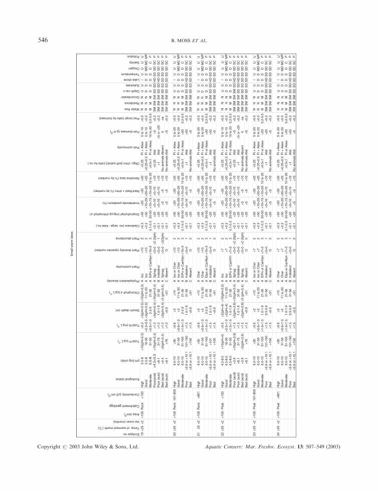
Sm

all w

arm

lake

s

19>

25<

2<

100

Roc

k<

100

Hig

h5.

5-8

<15

(pH

>5.

5)<

0.3

>3(

pH>

5.5)

<10

(pH

>5.

5)A

Iso

>10

2>

0.3

>50

>20

>30

>20

<0.

25P

i + A

bex

5 to

10

>0.

5U

UI

UU

UU

Goo

d5.

5-8

16-3

0>

0.3<

0.5

>3(

pH>

5.5)

11 to

20

AIs

o>

102

>0.

3>

50>

15<

20>

20<

30>

20>

0.25

<0.

5P

i + A

bex

5 to

10

>0.

5D

DD

DM

DM

CM

PM

oder

ate

5.5-

831

-50

>0.

5<1.

02-

2.9

21-3

0A

ElP

o or

Can

Nym

<10

>3

30.

1-0.

320

-50

>10

<15

>10

<20

10 to

20

>0.

5<1

Pi o

r A

bex

10 to

20

0.2-

0.5

MM

MNN

N NN

ND

DD

DD

CP

Poo

r(ac

id)

>4.

5<5.

5<

15(p

H<

5.4)

>1.

0>

3(pH

<5.

4)<

10(p

H<

5.4)

AS

phag

<3>

0>

2 (S

ph)

<0.

1>

20>

5<10

>5<

10<

10<

0.25

Altd

<5

<0.

2S

MS

MS

MS

DS

DH

DS

DS

DS

CP

Poo

r (e

utr)

>8.

151

-75

>1.

01.

0-1.

931

-50

BIn

dist

inct

<3>

01

<0.

1>

20>

5<10

>5<

10<

10>

1A

ltd<

5 or

>20

<0.

2S

MS

MS

MS

DS

DH

DS

DS

DS

CP

Bad

(ac

id)

<4.

4<

5(pH

<5.

4)>

1.0

>3(

pH<

5.4)

<5

(pH

<5.

4)A

Sph

ag<

3>0

>2(

Sph

)<

0.1

>20

<5

<5

<10

No

anim

als

Abs

ent

0na

SM

SM

SM

SD

SD

SD

SD

SD

SC

PB

ad (

eutr

)>

8.1

>76

>1.

0<

0.9

>51

CA

bsen

tO

0<

0.1

>20

<5

<5

<10

No

anim

als

Altd

<5

<0.

2S

MS

MS

MS

DS

DS

DS

DS

DS

CP

20>

25<

2<

100

Roc

k10

1-80

0H

igh

6.0-

10<

30<

0.6

>3

<10

AIs

o or

Cha

r>

102

>0.

3>

50>

20>

30>

20<

0.25

Pi +

Abe

x5

to 2

0>

0.5

UI

UG

ood

6.0-

1031

-50

>0.

6<1.

0>

311

to 2

0A

Iso

or C

har

>10

2>

0.3

>50

>15

<20

>20

<30

>20

>0.

25<

0.5

Pi +

Abe

x5

to 2

0>

0.5

DD

DM

DM

CM

PM

oder

ate

6.0-

1051

-100

>1.

0<1.

52-

2.9

21-3

0A

ElP

o or

Can

Ny m

<10

>3

30.

1-0.

320

-50

>10

<15

>10

<20

10 to

20

>0.

5<1

Pi o

r A

bex

>20

0.2-

0.5

MM

MD

DD

DD

CP

Poo

r<

5.9

or >

10.1

101-

150

>1.

51.

0-1.

931

-50

BIn

dist

inct

<3>

01

<0.

1<

20>

5<10

>5<

10<

10>

1A

ltd>

20<

0.2

SM

SM

SM

SD

SD

HD

SD

SD

SC

PB

ad<

5.9

or >

10.1

>15

0>

1.5

<0.

9>

51C

Abs

ent

O0

<0.

1<

20<

5<

5<

10N

o an

imal

sA

ltd<

5<

0.2

SM

SM

SM

SD

SD

SD

SD

SD

SC

P

2125

<2

<10

0R

ock

>80

1H

igh

6.0-

10<

30<

0.6

>3

<10

AC

har

>10

2>

0.3

>50

>20

>30

>20

<0.

25P

i +A

bex

5 to

20

>0.

5U

IU

Goo

d6.

0-10

31-5

0>

0.6<

1.0

>3

11 to

20

AC

har

>10

2>

0.3

>50

>15

<20

>20

<30

>20

>0.

25<

0.5

Pi +

Abe

x5

to 2

0>

0.5

DD

DM

DM

CM

PM

oder

ate

6.0-

1051

-100

>1.

0<1.

52-

2.9

21-3

0A

Elp

o or

Can

Nym

<10

>3

30.

1-0.

320

-50

>10

<15

>10

<20

10 to

20

>0.

5<1

Pi o

r A

bex

>20

0.2-

0.5

MM

MD

DD

DD

CP

Poo

r<

5.9

or >

10.1

>10

1>

1.5

1.0-

1.9

31-5

0B

Indi

stin

ct<

3>0

1<

0.1

<20

>5<

10>

5<10

<10

>1

Altd

>20

<0.

2S

MS

MS

MS

DS

DH

DS

DS

DS

CP

Bad

<5.

9 or

>10

.1>

150

>1.

5<

0.9

>51

CA

bsen

tO

0<

0.1

<20

<5

<5

<10

No

anim

als

Altd

<5

<0.

2S

MS

MS

MS

DS

DS

DS

DS

DS

CP

22>

25<

2<

100

Pea

t<

100

Hig

h4.

0-8.

0<

15(p

H>

4)<

0.5

>2(

pH>

4)<

10(p

H>

5.5)

AIs

o>

72

>0.

3>

50>

20>

30>

20<

0.25

Pi +

Abe

x5

to 1

0>

0.5

UI

UG

ood

4.0-

8.0

16-3

0>

0.5<

1.0

>2(

pH>

4)11

to 2

0A

Iso

>7

2>

0.3

>50

>15

<20

>20

<30

>20

>0.

25<

0.5

Pi +

Abe

x5

to 1

0>

0.5

DD

DM

DM

CM

PM

oder

ate

4.0-

8.0

31-5

0>

1.0<

1.5

1.0-

1.9

21-3

0A

ElP

o or

Can

NY

m<

7>3

30.

1-0.

320

-50

>10

<15

>10

<20

10 to

20

>0.

5<1

Pi o

r A

bex

10 to

20

0.2-

0.5

MM

MD

DD

DD

CP

Poo

r (a

cid)

<3.

9<

15(p

H<

3.9)

>1.

5>

2(pH

<3.

9)<

10(p

H<

5.4)

AS

phag

<3>

0>

2 (S

ph)

<0.

1>

20>

5<10

>5<

10<

10<

0.25

Altd

<5

<0.

2S

MS

MS

MS

MS

DH

DS

DS

DS

CP

Poo

r (e

utr)

>8.

151

-75

>1.

51.

0-1.

931

-50

BIn

dist

inct

<3>

01

<0.

1>

20>

5<10

>5<

10<

10>

1A

ltd<

5 or

>20

<0.

2S

MS

MS

MS

DS

DH

DS

DS

DS

CP

Bad

(ac

id)

<3.

9<

5(pH

<3.

9)>

1.5

>2(

pH<

3.9)

<5

(pH

<5.

4)A

Sph

ag<

3>0

>2

(Sph

)<

0.1

>20

<5

<5

<10

No

anim

als

Abs

ent

0na

SM

SM

SM

SD

SD

SD

SD

SD

SC

PB

ad (

eutr

)>

8.1

>76

>1.

5<

0.9

>51

CA

bsen

tO

0<

0.1

>20

<5

<5

<10

No

anim

als

Altd

<5

<0.

2S

MS

MS

MS

DS

DS

DS

DS

DS

CP

23>

25<

2<

100

Pea

t10

1-80

0H

igh

6.0-

10<

30<

0.6

>2

<10

AIs

o or

Cha

r>

72

>0.

3>

50>

20>

30>

20<

0.25

Pi +

Abe

x5

to 2

0>

0.5

UI

UG

ood

6.0-

1031

-50

>0.

6<1.

0>

211

to 2

0A

Iso

or C

har

>7

2>

0.3

>50

>15

<20

>20

<30

>20

>0.

25<

0.5

Pi +

Abe

x5

to 2

0>

0.5

DD

DM

DM

CM

PM

oder

ate

6.0-

1051

-100

>1.

0<1.

51.

0-1.

921

-30

AE

lPo

or C

anN

ym<

7>3

30.

1-0.

320

-50

>10

<15

>10

<20

10 to

20

>0.

5<1

Pi o

r A

bex

>20

0.2-

0.5

MM

MD

DD

DD

CP

Poo

r<

5.9

or >

10.1

101-

150

>1.

50.

5-0.

931

-50

BIn

dist

inct

<3>

01

<0.

1<

20>

5<10

>5<

10<

10>

1A

ltd>

20<

0.2

SM

SM

SM

SD

SD

HD

SD

SD

SC

PB

ad<

5.9

or >

10.1

>15

0>

1.5

<0.

5>

51C

Abs

ent

O0

<0.

1<

20<

5<

5<

10N

o an

imal

sA

ltd<

5<

0.2

SM

SM

SM

SD

SD

SD

SD

SD

SC

P

24>

25<

2<

100

Pea

t>

801

Hig

h6.

0-10

<30

<0.

6>

2<

10A

Cha

r>

72

>0.

3>

50>

20>

30>

20<

0.25

Pi +

Abe

x5

to 2

0>

0.5

UI

UG

ood

6.0-

1031

-50

>0.

6<1.

0>

211

to 2

0A

Cha

r>

72

>0.

3>

50>

15<

20>

20<

30>

20>

0.25

<0.

5P

i + A

bex

5 to

20

>0.

5D

DD

MD

MC

MP

Mod

erat

e6.

0-10

51-1

00>

1.0<

1.5

1.0-

1.9

21-3

0A

Elp

o or

Can

Nym

<7>

33

0.1-

0.3

20-5

0>

10<

15>

10<

2010

to 2

0>

0.5<

1P

i or

Abe

x>

200.

2-0.

5M

MM

DD

DD

DC

PP

oor

<5.

9 or

>10

.110

1-15

0>

1.5

0.5-

0.9

31-5

0B

Indi

stin

ct<

3>0

1<

0.1

<20

>5<

10>

5<10

<10

>1

Altd

>20

<0.

2S

MS

MS

MS

DS

DH

DS

DS

DS

CP

Bad

<5.

9 or

>10

.1>

150

>1.

5<

0.5

>51

CA

bsen

tO

0<

0.1

<20

<5

<5

<10

No

anim

als

Altd

<5

<0.

2S

MS

MS

MS

DS

DS

DS

DS

DS

CP

Groundwater

Oxygen

Salinity

Pollution

Depth var.n

Substrate

Lake shore

Temperature



Water flow

Residence




Fish community

Plant abundance






Plant community


pH (log units)

Total P (µg L-1)

Total N (mg L-1)

Secchi depth (m)


Ice cover (months)

Ecotype no.

Ecological status

Area (km2)

Catchment geology


UU

UU

DN

NN N

NN

UU

UU

DN

NN N

NN

UU

UU

DN

NN N

NN

UU

UU

DN

NN N

NN

UU

UU

DN

NN N

NN

B. MOSS ET AL.546


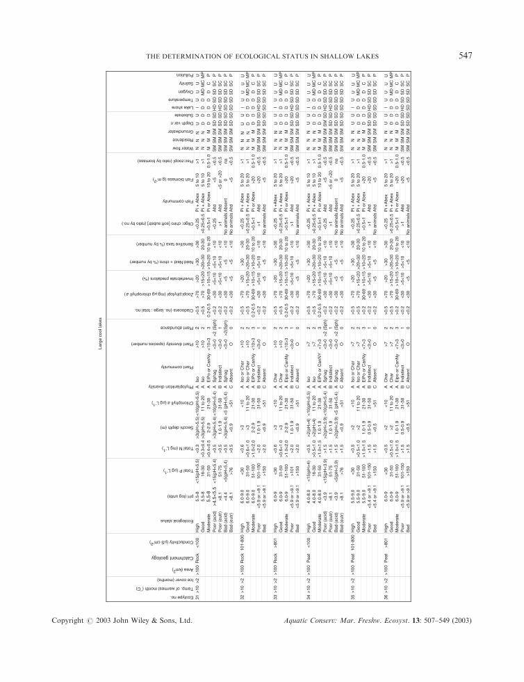
Larg

e co

ol la

kes

31>

10>

2>

100

Roc

k<

100

Hig

h5.

5-8

<15

(pH

>5.

5)<

0.3

>3(

pH>

5.5)

<10

(pH

>5.

5)A

Iso

>10

2>

0.5

>70

>20

>30

>30

<0.

25P

i + A

bex

5 to

10

>1

NN

NN

NN

UU

IU

UU

U

N N NN

NN

NN

NN

NN

N

NN

NN

NU U U

UU

U

Goo

d5.

5-8

16-3

0>

0.3<

0.4

>3(

pH>

5.5)

11 to

20

AIs

o>

102

>0.

5>

70>

15<

20>

20<

3020

-30

>0.

25<

0.5

Pi +

Abe

x5

to 1

0>

1D

DD

DM

DM

CM

PM

oder

ate

5.5-

831

-50

>0.

4<0.

52-

2.9

21-3

0A

ElP

o or

Can

Ny

<10

>3

30.

2-0.

530

-69

>10

<15

>10

<20

10 to

20

>0.

5<1

Pi o

r A

bex

10 to

20

0.5-

1.0

MM

MD

DD

DD

CP

Poo

r (a

cid)

>4.

5<5.

5<

15(p

H<

5.4)

>0.

5>

3(pH

<5.

4)<

10(p

H<

5.4)

AS

phag

<3>

0>

2 (S

ph)

<0.

2<

30>

5<10

>5<

10<

10<

0.25

Altd

<5

<0.

5S

MS

MS

MS

DS

DH

DS

DS

DS

CP

Poo

r (e

utr)

>8.

151

-75

>0.

51.

0-1.

931

-50

BIn

dist

inct

<3>

01

<0.

2<

30>

5<10

>5<

10<

10>

1A

ltd<

5 or

>20

<0.

5S

MS

MS

MS

DS

DH

DS

DS

DS

CP

Bad

(ac

id)

<4.

4<

5(pH

<5.

4)>

0.5

>3(

pH<

5.4)

<5

(pH

<5.

4)A

Sph

ag<

3>0

>2(

Sph

)<

0.2

<30

<5

<5

<10

No

anim

als

Abs

ent

0na

SM

SM

SM

SD

SD

SD

SD

SD

SC

PB

ad (

eutr

)>

8.1

>76

>0.

5<

0.9

>51

CA

bsen

tO

0<

0.2

<30

<5

<5

<10

No

anim

als

Altd

<5

<0.

5S

MS

MS

MS

DS

DS

DS

DS

DS

CP

32>

10>

2>

100

Roc

k10

1-80

0H

igh

6.0-

9.0

<30

<0.

6>

3<

10A

Iso

or C

har

>10

2>

0.5

>70

>20

>30

>30

<0.

25P

i + A

bex

5 to

20

>1

UI

UG

ood

6.0-

9.0

31-5

0>

0.6<

1.0

>3

11 to

20

AIs

o or

Cha

r>

102

>0.

5>

70>

15<

20>

20<

3020

-30

>0.

25<

0.5

Pi +

Abe

x5

to 2

0>

1D

DD

DM

DM

CM

PM

oder

ate

6.0-

9.0

51-1

00>

1.0<

2.0

2-2.

921

-30

AE

lPo

or C

anN

y<

10>

33

0.2-

0.5

30-6

9>

10<

15>

10<

2010

to 2

0>

0.5<

1P

i or

Abe

x>

200.

5-1.

0M

MM

DD

DD

DC

PP

oor

<5.

9 or

>9.

110

1-15

0>

2.0

1.0-

1.9

31-5

0B

Indi

stin

ct<

3>0

1<

0.2

<30

>5<

10>

5<10

<10

>1

Altd

>20

<0.

5S

MS

MS

MS

DS

DH

DS

DS

DS

CP

Bad

<5.

9 or

>9.

1>

150

>2.

0<

0.9

>51

CA

bsen

tO

0<

0.2

<30

<5

<5

<10

No

anim

als

Altd

<5

<0.

5S

MS

MS

MS

DS

DS

DS

DS

DS

CP

33>

10>

2>

100

Roc

k>

801

Hig

h6.

0-9

<30

<0.

6>

3<

10A

Cha

r>

102

>0.

5>

70>

20>

30>

30<

0.25

Pi +

Abe

x5

to 2

0>

1U

IU

UU

UG

ood

6.0-

931

-50

>0.

6<1.

0>

311

to 2

0A

Cha

r>

102

>0.

5>

70>

15<

20>

20<

3020

-30

>0.

25<

0.5

Pi +

Abe

x5

to 2

0>

1D

DD

DM

DM

CM

PM

oder

ate

6.0-

951

-100

>1.

0<2.

02-

2.9

21-3

0A

Elp

o or

Can

Ny

<10

>3

30.

2-0.

530

-69

>10

<15

>10

<20

10 to

20

>0.

5<1

Pi o

r A

bex

>20

0.5-

1.0

MM

MD

DD

DD

CP

Poo

r<

5.9

or >

9.1

>10

1>

2.0

1.0-

1.9

31-5

0B

Indi

stin

ct<

3>0

1<

0.2

<30

>5<

10>

5<10

<10

>1

Altd

>20

<0.

5S

MS

MS

MS

DS

DH

DS

DS

DS

CP

Bad

<5.

9 or

>9.

1>

150

>2.

0<

0.9

>51

CA

bsen

tO

0<

0.2

<30

<5

<5

<10

No

anim

als

Altd

<5

<0.

5S

MS

MS

MS

DS

DS

DS

DS

DS

CP

34>

10>

2>

100

Pea

t<

100

Hig

h4.

0-8.

0<

15(p

H>

4)<

0.5

>2(

pH>

4)<

10(p

H>

5.5)

AIs

o>

72

>0.

5>

70>

20>

30>

30<

0.25

Pi +

Abe

x5

to 1

0>

1U

IU

UU

U

UU

U

Goo

d4.

0-8.

016

-30

>0.

5<1.

0>

2(pH

>4)

11 to

20

AIs

o>

72

>0.

5>

70>

15<

20>

20<

3020

-30

>0.

25<

0.5

Pi +

Abe

x5

to 1

0>

1D

D

NN

NN

NN

U

NN

NN

NN

UD

DD

MD

MC

MP

Mod

erat

e4.

0-8.

031

-50

>1.

0<1.

51.

0-1.

921

-30

AE

lPo

or C

anN

Y<

7>3

30.

2-0.

530

-69

>10

<15

>10

<20

10 to

20

>0.

5<1

Pi o

r A

bex

10 to

20

0.5-

1.0

MM

MD

DD

DD

CP

Poo

r (a

cid)

<3.

9<

15(p

H<

3.9)

>1.

5>

2(pH

<3.

9)<

10(p

H<

5.4)

AS

phag

<3>

0>

2 (S

ph)

<0.

2<

30>

5<10

>5<

10<

10<

0.25

Altd

<5

<0.

5S

MS

MS

MS

MS

DH

DS

DS

DS

CP

Poo

r (e

utr)

>8.

151

-75

>1.

51.

0-1.

931

-50

BIn

dist

inct

<3>

01

<0.

2<

30>

5<10

>5<

10<

10>

1A

ltd<

5 or

>20

<0.

5S

MS

MS

MS

DS

DH

DS

DS

DS

CP

Bad

(ac

id)

<3.

9<

5(pH

<3.

9)>

1.5

>2(

pH<

3.9)

<5

(pH

<5.

4)A

Sph

ag<

3>0

>2

(Sph

)<

0.2

<30

<5

<5

<10

No

anim

als

Abs

ent

0na

SM

SM

SM

SD

SD

SD

SD

SD

SC

PB

ad (

eutr

)>

8.1

>76

>1.

5<

0.9

>51

CA

bsen

tO

0<

0.2

<30

<5

<5

<10

No

anim

als

Altd

<5

<0.

5S

MS

MS

MS

DS

DS

DS

DS

DS

CP

35>

10>

2>

100

Pea

t10

1-80

0H

igh

5.5-

9.0

<30

<0.

5>

2<

10A

Iso

or C

har

>7

2>

0.5

>70

>20

>30

>30

<0.

25P

i + A

bex

5 to

20

>1

UI

UG

ood

5.5-

9.0

31-5

0>

0.5<

1.0

>2

11 to

20

AIs

o or

Cha

r>

72

>0.

5>

70>

15<

20>

20<

3020

-30

>0.

25<

0.5

Pi +

Abe

x5

to 2

0>

1D

DD

MD

MC

MP

Mod

erat

e5.

5-9.

051

-100

>1.

0<1.

51.

0-1.

921

-30

AE

lPo

or C

anN

y<

7>3

3>

0.2

30-6

9>

10<

15>

10<

2010

to 2

0>

0.5<

1P

i or

Abe

x>

200.

5-1.

0M

MM

DD

DD

DC

PP

oor

<5.

4 or

>9.

110

1-15

0>

1.5

0.5-

0.9

31-5

0B

Indi

stin

ct<

3>0

1<

0.2

<30

>5<

10>

5<10

<10

>1

Altd

>20

<0.

5S

MS

MS

MS

DS

DH

DS

DS

DS

CP

Bad

<5.

4 or

>9.

1>

150

>1.

5<

0.5

>51

CA

bsen

tO

0<

0.2

<30

<5

<5

<10

No

anim

als

Altd

<5

<0.

5S

MS

MS

MS

DS

DS

DS

DS

DS

CP

36>

10>

2>

100

Pea

t>

801

Hig

h6.

0-9

<30

<0.

5>

2<

10A

Cha

r>

72

>0.

5>

70>

20>

30>

30<

0.25

Pi +

Abe

x5

to 2

0>

1U

IU

UU

UG

ood

6.0-

931

-50

>0.

5<1.

0>

211

to 2

0A

Cha

r>

72

>0.

5>

70>

15<

20>

20<

3020

-30

>0.

25<

0.5

Pi +

Abe

x5

to 2

0>

1D

DD

DM

DM

CM

PM

oder

ate

6.0-

951

-100

>1.

0<1.

51.

0-1.

921

-30

AE

lpo

or C

anN

y<

7>3

3>

0.2

30-6

9>

10<

15>

10<

2010

to 2

0>

0.5<

1P

i or

Abe

x>

200.

5-1.

0M

MM

DD

DD

DC

PP

oor

<5.

9 or

>9.

110

1-15

0>

1.5

0.5-

0.9

31-5

0B

Indi

stin

ct<

3>0

1<

0.2

<30

>5<

10>

5<10

<10

>1

Altd

>20

<0.

5S

MS

MS

MS

DS

DH

DS

DS

DS

CP

Bad

<5.

9 or

>9.

1>

150

>1.

5<

0.5

>51

CA

bsen

tO

0<

0.2

<30

<5

<5

<10

No

anim

als

Altd

<5

<0.

5S

MS

MS

MS

DS

DS

DS

DS

DS

CP

Groundwater

Oxygen

Salinity

Pollution

Depth var.n

Substrate

Lake shore

Temperature



Water flow

Residence




Fish community

Plant abundance

Cladocera (no. large : total no.





Plant community


pH (log units)

Total P (µg L-1)

Total N (mg L-1)

Secchi depth (m)


Ice cover (months)

Ecotype no.

Ecological status

Area (km2)

Catchment geology




Larg

e te

mpe

rate

lake

s

37>

10<

25<

2>

100

Roc

k<

100

Hig

h5.

5-8

<15

(pH

>5.

5)<

0.3

>3(

pH>

5.5)

<10

(pH

>5.

5)A

Iso

>10

2>

0.5

>70

>20

>30

>20

<0.

25P

i + A

bex

5 to

10

>1

NN

N NU

UI

UU

UU

Goo

d5.

5-8

16-3

0>

0.3<

0.4

>3(

pH>

5.5)

11 to

20

AIs

o>

102

>0.

5>

70>

15<

20>

20<

30>

20>

0.25

<0.

5P

i + A

bex

5 to

10

>1

NN

DD

DD

MD

MC

MP

Mod

erat

e5.

5-8

31-5

0>

0.4<

0.5

2-2.

921

-30

AE

lPo

or C

anN

y<

10>

33

0.2-

0.5

30-6

9>

10<

15>

10<

2010

to 2

0>

0.5<

1P

i or

Abe

x10

to 2

00.

5-1.

0M

MM

DD

DD

DC

PP

oor

(aci

d)>

4.5<

5.5

<15

(pH

<5.

4)>

0.5

>3(

pH<

5.4)

<10

(pH

<5.

4)A

Sph

ag<

3>0

>2

(Sph

)<

0.2

<30

>5<

10>

5<10

<10

<0.

25A

ltd<

5<

0.5

SM

SM

SM

SD

SD

HD

SD

SD

SC

PP

oor

(eut

r)>

8.1

51-7

5>

0.5

1.0-

1.9

31-5

0B

Indi

stin

ct<

3>0

1<

0.2

<30

>5<

10>

5<10

<10

>1

Altd

<5

or >

20<

0.5

SM

SM

SM

SD

SD

HD

SD

SD

SC

PB

ad (

acid

)<

4.4

<5(

pH<

5.4)

>0.

5>

3(pH

<5.

4)<

5 (p

H<

5.4)

AS

phag

<3>

0>

2(S

ph)

<0.

2<

30<

5<

5<

10N

o an

imal

sA

bsen

t0

naS

MS

MS

MS

DS

DS

DS

DS

DS

CP

Bad

(eu

tr)

>8.

1>

76>

0.5

<0.

9>

51C

Abs

ent

O0

<0.

2<

30<

5<

5<

10N

o an

imal

sA

ltd<

5<

0.5

SM

SM

SM

SD

SD

SD

SD

SD

SC

P

38>

10<

25<

2>

100

Roc

k10

1-80

0H

igh

6.0-

9.0

<30

<0.

6>

3<

10A

Iso

or C

har

>10

2>

0.5

>70

>20

>30

>20

<0.

25P

i + A

bex

5 to

20

>1

NN

NU

UI

UU

UU

Goo

d6.

0-9.

031

-50

>0.

6<1.

0>

311

to 2

0A

Iso

or C

har

>10

2>

0.5

>70

>15

<20

>20

<30

>20

>0.

25<

0.5

Pi +

Abe

x5

to 2

0>

1N

NN

DD

DD

MD

MC

MP

Mod

erat

e6.

0-9.

051

-100

>1.

0<2.

02-

2.9

21-3

0A

ElP

o or

Can

Ny

<10

>3

30.

2-0.

530

-69

>10

<15

>10

<20

10 to

20

>0.

5<1

Pi o

r A

bex

>20

0.5-

1.0

MM

MD

DD

DD

CP

Poo

r<

5.9

or >

9.1

101-

150

>2.

01.

0-1.

931

-50

BIn

dist

inct

<3>

01

<0.

2<

30>

5<10

>5<

10<

10>

1A

ltd>

20<

0.5

SM

SM

SM

SD

SD

HD

SD

SD

SC

PB

ad<

5.9

or >

9.1

>15

0>

2.0

<0.

9>

51C

Abs

ent

O0

<0.

2<

30<

5<

5<

10N

o an

imal

sA

ltd<

5<

0.5

SM

SM

SM

SD

SD

SD

SD

SD

SC

P

39>

10<

25<

2>

100

Roc

k>

801

Hig

h6.

0-9

<30

<0.

6>

3<

10A

Cha

r>

102

>0.

5>

70>

20>

30>

20<

0.25

Pi +

Abe

x5

to 2

0>

1N

NN

NN

UU

NN

NN

NN

U

NN

NN

NN

NN

NN

NN

U

IU

UU

U

UU

U

Goo

d6.

0-9

31-5

0>

0.6<

1.0

>3

11 to

20

AC

har

>10

2>

0.5

>70

>15

<20

>20

<30

>20

>0.

25<

0.5

Pi +

Abe

x5

to 2

0>

1N

DD

DD

MD

MC

MP

Mod

erat

e6.

0-9

51-1

00>

1.0<

2.0

2-2.

921

-30

AE

lpo

or C

anN

y<

10>

33

0.2-

0.5

30-6

9>

10<

15>

10<

2010

to 2

0>

0.5<

1P

i or

Abe

x>

200.

5-1.

0M

MM

DD

DD

DC

PP

oor

<5.

9 or

>9.

1>

101

>2.

01.

0-1.

931

-50

BIn

dist

inct

<3>

01

<0.

2<

30>

5<10

>5<

10<

10>

1A

ltd>

20<

0.5

SM

SM

SM

SD

SD

HD

SD

SD

SC

PB

ad<

5.9

or >

9.1

>15

0>

2.0

<0.

9>

51C

Abs

ent

O0

<0.

2<

30<

5<

5<

10N

o an

imal

sA

ltd<

5<

0.5

SM

SM

SM

SD

SD

SD

SD

SD

SC

P

40>

10<

25<

2>

100

Pea

t<

100

Hig

h4.

0-8.

0<

15(p

H>

4)<

0.5

>2(

pH>

4)<

10(p

H>

5.5)

AIs

o>

72

>0.

5>

70>

20>

30>

20<

0.25

Pi +

Abe

x5

to 1

0>

1U

IU

Goo

d4.

0-8.

016

-30

>0.

5<1.

0>

2(pH

>4)

11 to

20

AIs

o>

72

>0.

5>

70>

15<

20>

20<

30>

20>

0.25

<0.

5P

i + A

bex

5 to

10

>1

DD

DD

MD

MC

MP

Mod

erat

e4.

0-8.

031

-50

>1.

0<1.

51.

0-1.

921

-30

AE

lPo

or C

anN

Y<

7>3

30.

2-0.

530

-69

>10

<15

>10

<20

10 to

20

>0.

5<1

Pi o

r A

bex

10 to

20

0.5-

1.0

MM

MD

DD

DD

CP

Poo

r (a

cid)

<3.

9<

15(p

H<

3.9)

>1.

5>

2(pH

<3.

9)<

10(p

H<

5.4)

AS

phag

<3>

0>

2 (S

ph)

<0.

2<

30>

5<10

>5<

10<

10<

0.25

Altd

<5

<0.

5S

MS

MS

MS

MS

DH

DS

DS

DS

CP

Poo

r (e

utr)

>8.

151

-75

>1.

51.

0-1.

931

-50

BIn

dist

inct

<3>

01

<0.

2<

30>

5<10

>5<

10<

10>

1A

ltd<

5 or

>20

<0.

5S

MS

MS

MS

DS

DH

DS

DS

DS

CP

Bad

(ac

id)

<3.

9<

5(pH

<3.

9)>

1.5

>2(

pH<

3.9)

<5

(pH

<5.

4)A

Sph

ag<

3>0

>2

(Sph

)<

0.2

<30

<5

<5

<10

No

anim

als

Abs

ent

0na

SM

SM

SM

SD

SD

SD

SD

SD

SC

PB

ad (

eutr

)>

8.1

>76

>1.

5<

0.9

>51

CA

bsen

tO

0<

0.2

<30

<5

<5

<10

No

anim

als

Altd

<5

<0.

5S

MS

MS

MS

DS

DS

DS

DS

DS

CP

41>

10<

25<

2>

100

Pea

t10

1-80

0H

igh

5.5-

9.0

<30

<0.

5>

2<

10A

Iso

or C

har

>7

2>

0.5

>70

>20

>30

>20

<0.

25P

i + A

bex

5 to

20

>1

UI

UU

UU

Goo

d5.

5-9.

031

-50

>0.

5<1.

0>

211

to 2

0A

Iso

or C

har

>7

2>

0.5

>70

>15

<20

>20

<30

>20

>0.

25<

0.5

Pi +

Abe

x5

to 2

0>

1D

DD

DM

DM

CM

PM

oder

ate

5.5-

9.0

51-1

00>

1.0<

1.5

1.0-

1.9

21-3

0A

ElP

o or

Can

Ny

<7>

33

>0.

230

-69

>10

<15

>10

<20

10 to

20

>0.

5<1

Pi o

r A

bex

>20

0.5-

1.0

MM

MD

DD

DD

CP

Poo

r<

5.4

or >

9.1

101-

150

>1.

50.

5-0.

931

-50

BIn

dist

inct

<3>

01

<0.

2<

30>

5<10

>5<

10<

10>

1A

ltd>

20<

0.5

SM

SM

SM

SD

SD

HD

SD

SD

SC

PB

ad<

5.4

or >

9.1

>15

0>

1.5

<0.

5>

51C

Abs

ent

O0

<0.

2<

30<

5<

5<

10N

o an

imal

sA

ltd<

5<

0.5

SM

SM

SM

SD

SD

SD

SD

SD

SC

P

42>

10<

25<

2>

100

Pea

t>

801

Hig

h6.

0-9

<30

<0.

5>

2<

10A

Cha

r>

72

>0.

5>

70>

20>

30>

20<

0.25

Pi +

Abe

x5

to 2

0>

1U

UI

UU

UU

Goo

d6.

0-9

31-5

0>

0.5<

1.0

>2

11 to

20

AC

har

>7

2>

0.5

>70

>15

<20

>20

<30

>20

>0.

25<

0.5

Pi +

Abe

x5

to 2

0>

1D

DD

DM

DM

CM

PM

oder

ate

6.0-

951

-100

>1.

0<1.

51.

0-1.

921

-30

AE

lpo

or C

anN

y<

7>3

3>

0.2

30-6

9>

10<

15>

10<

2010

to 2

0>

0.5<

1P

i or

Abe

x>

200.

5-1.

0M

MM

DD

DD

DC

PP

oor

<5.

9 or

>9.

110

1-15

0>

1.5

0.5-

0.9

31-5

0B

Indi

stin

ct<

3>0

1<

0.2

<30

>5<

10>

5<10

<10

>1

Altd

>20

<0.

5S

MS

MS

MS

DS

DH

DS

DS

DS

CP

Bad

<5.

9 or

>9.

1>

150

>1.

5<

0.5

>51

CA

bsen

tO

0<

0.2

<30

<5

<5

<10

No

anim

als

Altd

<5

<0.

5S

MS

MS

MS

DS

DS

DS

DS

DS

CP

Groundwater

Oxygen

Salinity

Pollution

Depth var.n

Substrate

Lake shore

Temperature



Water flow

Residence




Fish community

Plant abundance






Plant community


pH (log units)

Total P (µg L-1)

Total N (mg L-1)

Secchi depth (m)


Ice cover (months)

Ecotype no.

Ecological status

Area (km2)

Catchment geology


B. MOSS ET AL.548


Larg

e w

arm

lake

s

43>

25<

2>

100

Roc

k<

100

Hig

h5.

5-8

<15

(pH

>5.

5)<

0.3

>3(

pH>

5.5)

<10

(pH

>5.

5)A

Iso

>10

2>

0.3

>50

>20

>30

>20

<0.

25P

i + A

bex

5 to

10

>0.

5N N

NN

NN

UU

IU

UU

UG

ood

5.5-

816

-30

0.3-

0.5

>3(

pH>

5.5)

11 to

20

AIs

o>

102

>0.

3>

50>

15<

20>

20<

30>

20>

0.25

<0.

5P

i + A

bex

5 to

10

>0.

5D

DD

DM

DM

CM

PM

oder

ate

5.5-

831

-50

0.5-

1.0

2-2.

921

-30

AE

lPo

or C

anN

y<

10>

33

0.1-

0.3

20-5

0>

10<

15>

10<

2010

to 2

0>

0.5<

1P

i or

Abe

x10

to 2

00.

2-0.

5M

MM

DD

DD

DC

PP

oor

(aci

d)4.

5-5.

5<

15(p

H<

5.4)

>1.

0>

3(pH

<5.

4)<

10(p

H<

5.4)

AS

phag

0-3

>2

(Sph

)<

0.1

>20

>5<

10>

5<10

<10

<0.

25A

ltd<

5<

0.2

SM

SM

SM

SD

SD

HD

SD

SD

SC

PP

oor

(eut

r)>

8.1

51-7

5>

1.0

1.0-

1.9

31-5

0B

Indi

stin

ct0-

31

<0.

1>

20>

5<10

>5<

10<

10>

1A

ltd<

5 or

>20

<0.

2S

MS

MS

MS

DS

DH

DS

DS

DS

CP

Bad

(ac

id)

<4.

4<

5(pH

<5.

4)>

1.0

>3(

pH<

5.4)

<5

(pH

<5.

4)A

Sph

ag0-

3>

2(S

ph)

<0.

1>

20<

5<

5<

10N

o an

imal

sA

bsen

t0

naS

MS

MS

MS

DS

DS

DS

DS

DS

CP

Bad

(eu

tr)

>8.

1>

76>

1.0

<0.

9>

51C

Abs

ent

O0

<0.

1>

20<

5<

5<

10N

o an

imal

sA

ltd<

5<

0.2

SM

SM

SM

SD

SD

SD

SD

SD

SC

P

44>

25<

2>

100

Roc

k10

1-80

0H

igh

6.0-

10<

30<

0.6

>3

<10

AIs

o or

Cha

r>

102

>0.

3>

50>

20>

30>

20<

0.25

Pi +

Abe

x5

to 2

0>

0.5

UI

UG

ood

6.0-

1031

-50

0.6-

1.0

>3

11 to

20

AIs

o or

Cha

r>

102

>0.

3>

50>

15<

20>

20<

30>

20>

0.25

<0.

5P

i + A

bex

5 to

20

>0.

5D

DD

MD

MC

MP

Mod

erat

e6.

0-10

51-1

001.

1-1.

52-

2.9

21-3

0A

ElP

o or

Can

Ny

<10

>3

30.

1-0.

320

-50

>10

<15

>10

<20

10 to

20

>0.

5<1

Pi o

r A

bex

>20

0.2-

0.5

MM

MD

DD

DD

CP

Poo

r<

5.9

or >

10.1

101-

150

>1.

51.

0-1.

931

-50

BIn

dist

inct

<3>

01

<0.

1<

20>

5<10

>5<

10<

10>

1A

ltd>

20<

0.2

SM

SM

SM

SD

SD

HD

SD

SD

SC

PB

ad<

5.9

or >

10.1

>15

0>

1.5

<0.

9>

51C

Abs

ent

O0

<0.

1<

20<

5<

5<

10N

o an

imal

sA

ltd<

5<

0.2

SM

SM

SM

SD

SD

SD

SD

SD

SC

P

45>

25<

2>

100

Roc

k>

801

Hig

h6.

0-10

<30

<0.

6>

3<

10A

Cha

r>

102

>0.

3>

50>

20>

30>

20<

0.25

Pi +

Abe

x5

to 2

0>

0.5

UI

UG

ood

6.0-

1031

-50

0.6-

1.0

>3

11 to

20

AC

har

>10

2>

0.3

>50

>15

<20

>20

<30

>20

>0.

25<

0.5

Pi +

Abe

x5

to 2

0>

0.5

DD

DM

DM

CM

PM

oder

ate

6.0-

1051

-100

1.0-

1.5

2-2.

921

-30

AE

lpo

or C

anN

y<

10>

33

0.1-

0.3

20-5

0>

10<

15>

10<

2010

to 2

0>

0.5<

1P

i or

Abe

x>

200.

2-0.

5M

MM

DD

DD

DC

PP

oor

<5.

9 or

>10

.1>

101

>1.

51.

0-1.

931

-50

BIn

dist

inct

<3>

01

<0.

1<

20>

5<10

>5<

10<

10>

1A

ltd>

20<

0.2

SM

SM

SM

SD

SD

HD

SD

SD

SC

PB

ad<

5.9

or >

10.1

>15

0>

1.5

<0.

9>

51C

Abs

ent

O0

<0.

1<

20<

5<

5<

10N

o an

imal

sA

ltd<

5<

0.2

SM

SM

SM

SD

SD

SD

SD

SD

SC

P

46>

25<

2>

100

Pea

t<

100

Hig

h4.

0-8.

0<

15(p

H>

4)<

0.5

>2(

pH>

4)<

10(p

H>

5.5)

AIs

o>

72

>0.

3>

50>

20>

30>

20<

0.25

Pi +

Abe

x5

to 1

0>

0.5

UI

UG

ood

4.0-

8.0

16-3

00.

5-1.

0>

2(pH

>4)

11 to

20

AIs

o>

72

>0.

3>

50>

15<

20>

20<

30>

20>

0.25

<0.

5P

i + A

bex

5 to

10

>0.

5D

DD

MD

MC

MP

Mod

erat

e4.

0-8.

031

-50

1.1-

1.5

1.0-

1.9

21-3

0A

ElP

o or

Can

NY

<7>

33

0.1-

0.3

20-5

0>

10<

15>

10<

2010

to 2

0>

0.5<

1P

i or

Abe

x10

to 2

00.

2-0.

5M

MM

DD

DD

DC

PP

oor

(aci

d)<

3.9

<15

(pH

<3.

9)>

1.5

>2(

pH<

3.9)

<10

(pH

<5.

4)A

Sph

ag<

3>0

>2

(Sph

)<

0.1

>20

>5<

10>

5<10

<10

<0.

25A

ltd<

5<

0.2

SM

SM

SM

SM

SD

HD

SD

SD

SC

PP

oor

(eut

r)>

8.1

51-7

5>

1.5

1.0-

1.9

31-5

0B

Indi

stin

ct<

3>0

1<

0.1

>20

>5<

10>

5<10

<10

>1

Altd

<5

or >

20<

0.2

SM

SM

SM

SD

SD

HD

SD

SD

SC

PB

ad (

acid

)<

3.9

<5(

pH<

3.9)

>1.

5>

2(pH

<3.

9)<

5 (p

H<

5.4)

AS

phag

<3>

0>

2 (S

ph)

<0.

1>

20<

5<

5<

10N

o an

imal

sA

bsen

t0

naS

MS

MS

MS

DS

DS

DS

DS

DS

CP

Bad

(eu

tr)

>8.

1>

76>

1.5

<0.

9>

51C

Abs

ent

O0

<0.

1>

20<

5<

5<

10N

o an

imal

sA

ltd<

5<

0.2

SM

SM

SM

SD

SD

SD

SD

SD

SC

P

47>

25<

2>

100

Pea

t10

1-80

0H

igh

6.0-

10<

30<

0.6

>2

<10

AIs

o or

Cha

r>

72

>0.

3>

50>

20>

30>

20<

0.25

Pi +

Abe

x5

to 2

0>

0.5

UI

UG

ood

6.0-

1031

-50

0.6-

1.0

>2

11 to

20

AIs

o or

Cha

r>

72

>0.

3>

50>

15<

20>

20<

30>

20>

0.25

<0.

5P

i + A

bex

5 to

20

>0.

5D

DD

MD

MC

MP

Mod

erat

e6.

0-10

51-1

001.

0-1.

51.

0-1.

921

-30

AE

lPo

or C

anN

y<

7>3

30.

1-0.

320

-50

>10

<15

>10

<20

10 to

20

>0.

5<1

Pi o

r A

bex

>20

0.2-

0.5

MM

MD

DD

DD

CP

Poo

r<

5.9

or >

10.1

101-

150

>1.

50.

5-0.

931

-50

BIn

dist

inct

<3>

01

<0.

1<

20>

5<10

>5<

10<

10>

1A

ltd>

20<

0.2

SM

SM

SM

SD

SD

HD

SD

SD

SC

PB

ad<

5.9

or >

10.1

>15

0>

1.5

<0.

5>

51C

Abs

ent

O0

<0.

1<

20<

5<

5<

10N

o an

imal

sA

ltd<

5<

0.2

SM

SM

SM

SD

SD

SD

SD

SD

SC

P

48>

25<

2>

100

Pea

t>

801

Hig

h6.

0-10

<30

<0.

6>

2<

10A

Cha

r>

72

>0.

3>

50>

20>

30>

20<

0.25

Pi +

Abe

x5

to 2

0>

0.5

UI

UG

ood

6.0-

1031

-50

0.6-

1.0

>2

11 to

20

AC

har

>7

2>

0.3

>50

>15

<20

>20

<30

>20

>0.

25<

0.5

Pi +

Abe

x5

to 2

0>

0.5

DD

DM

DM

CM

PM

oder

ate

6.0-

1051

-100

1.0-

1.5

1.0-

1.9

21-3

0A

Elp

o or

Can

Ny

<7>

33

0.1-

0.3

20-5

0>

10<

15>

10<

2010

to 2

0>

0.5<

1P

i or

Abe

x>

200.

2-0.

5M

MM

DD

DD

DC

PP

oor

<5.

9 or

>10

.110

1-15

0>

1.5

0.5-

0.9

31-5

0B

Indi

stin

ct<

3>0

1<

0.1

<20

>5<

10>

5<10

<10

>1

Altd

>20

<0.

2S

MS

MS

MS

DS

DH

DS

DS

DS

CP

Bad

<5.

9 or

>10

.1>

150

>1.

5<

0.5

>51

CA

bsen

tO

0<

0.1

<20

<5

<5

<10

No

anim

als

Altd

<5

<0.

2S

MS

MS

MS

DS

DS

DS

DS

DS

CP

Groundwater

Oxygen

Salinity

Pollution

Depth var.n

Substrate

Lake shore

Temperature



Water flow

Residence




Fish community

Plant abundance






Plant community


pH (log units)

Total P (µg L-1)

Total N (mg L-1)

Secchi depth (m)


Ice cover (months)

Ecotype no.

Ecological status

Area (km2)

Catchment geology


N NN

NN

NU

UU

UD

N NN

NN

NU

UU

UD

N NN

NN

NU

UU

UD

N NN

NN

NU

UU

UD

N NN

NN

NU

UU

UD



Documents

The determination of ecological status in shallow lakes ...pcpelagic/s/Moss et al 2003(2).pdf · ABSTRACT 1. The European Water Framework Directive requires the determination of ecological