Embed Size (px)
Citation preview

WORKING PAPER The Determinants of Family and Individual Migration: A Case-Study of Rural Bangladesh Randall S. Kuhn July 2005 Research Program on Population Processes POP2005-05 Population Aging Center PAC2005-04
The Determinants of Family and Individual Migration: A Case-Study of Rural Bangladesh
Randall S. Kuhn* Population Program – Institute of Behavioral Science
October 2004
* The author gratefully acknowledges the support of the International Pre-Dissertation Fellowship of the Social Science Research Council (supported by Ford Foundation and American Council of Learned Societies); the J. William Fulbright Scholarship (funded by United States Information Agency, administered by Institute for International Education); the Population Council Dissertation Fellowship in the Social Sciences; the Mellon Fund for Research in Population in Developing Countries; and the University of Colorado Population Aging Center (funded by National Institute on Aging). Many colleagues provided valuable commentaries on earlier versions of the paper, including Jane Menken, Douglas Massey, Leah Vanwey, Robert Retherford, Jeroen van Ginneken, Lynn Karoly, Erin Trapp, Julie DaVanzo, and Richard Rogers. Most of all, the author wishes to thank the research and technical staff of the Matlab Health and Demographic Surveillance Unit at ICDDR,B: International Centre for Health and Population Research, and the patient and thoughtful citizens of Matlab. Author’s Contact Information Randall Kuhn University of Colorado IBS Population Program - 484 UCB Boulder, CO 80309-0484 [email protected] (303) 492-1476 / Fax: (303) 492-6924
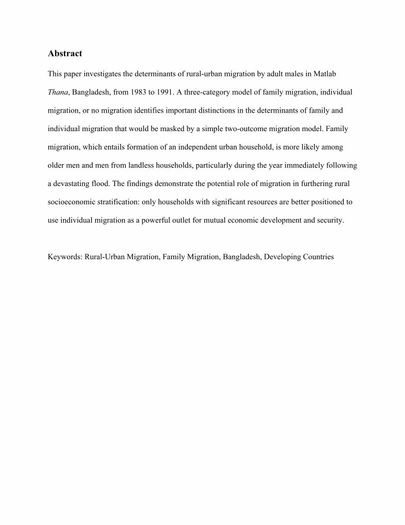
Abstract
This paper investigates the determinants of rural-urban migration by adult males in Matlab
Thana, Bangladesh, from 1983 to 1991. A three-category model of family migration, individual
migration, or no migration identifies important distinctions in the determinants of family and
individual migration that would be masked by a simple two-outcome migration model. Family
migration, which entails formation of an independent urban household, is more likely among
older men and men from landless households, particularly during the year immediately following
a devastating flood. The findings demonstrate the potential role of migration in furthering rural
socioeconomic stratification: only households with significant resources are better positioned to
use individual migration as a powerful outlet for mutual economic development and security.
Keywords: Rural-Urban Migration, Family Migration, Bangladesh, Developing Countries
I. Introduction In attempting to understand migration, social scientists often ignore the heterogeneity in both
migration pattern and motivation that exists in many sending populations. Migration can
maximize the welfare of the migrant as well as the members of a larger family unit. Migration
can involve individuals moving alone as well as entire families. Motives and practices are both
conditioned by life course transitions, as well as characteristics of the migrant and household.
Numerous review articles acknowledge these differences, and some papers find empirical
evidence of multiple motivations for migration in the same population. Yet few papers have
asked how the determinants of migration might differ between different types of migrants within
the same population.
This paper addresses the diversity of motivations for rural-urban migration by men in a
rural area of Bangladesh in two ways. It looks separately at migration before and after marriage,
a life event that both reduces the likelihood of migration and changes the nature of the migration
decision. It also separates the migration of married men into migration alone (referred to as
“individual migration”) or with conjugal family members (referred to as “family migration”). An
iterative cycle of qualitative fieldwork and quantitative analysis has determined that a simple
mover-stayer model of rural-urban migration in this context would mask heterogeneity in the
determinants of family and individual migration. For instance, a simple negative relationship
between land holdings and migration propensity common in many settings could mask a
tendency for family migration to be far more likely among men from landless households.
Results from a standard two-outcome, mover-stayer model are thus compared against
those of a three-outcome model where married men can choose to stay, to migrate as an
individual, or to migrate with a family. Expected differences in the age-, land-, and education
profile of family and individual migrants will suggest substantial differences between the two
2
groups.
The analysis also studies migration patterns in the year immediately following a major
flood. The likelihood of family and individual migration should increase following such a major
ecological and economic catastrophe, yet the characteristics of those practicing family and
individual migration following the flood should diverge considerably.
Each such result should give migration analysts pause to consider whether the purported
opportunities and benefits of migration will apply evenly to all sub-groups within a particular
community. This is very different from suggesting that some migrants will succeed or fail, and
some households will benefit or not. The results of this paper will suggest that family migrants
may enter the migration process coming from substantially more disadvantaged backgrounds and
having substantially fewer prospects than individual migrants. The systematic promise of
negative migration outcomes among certain sub-groups should also give policymakers reason to
redouble their efforts to secure rural livelihoods for at-risk households through pathways other
than migration.
The following section addresses the diversity versus heterogeneity issue in the literature
on the detminants of migration. After discussing the context of rural-urban migration in
Bangladesh, I introduce the Matlab Health and Demographic Surveillance System (HDSS) data,
which are ideally suited to prospectively identifying individual and family migration behavior
and offer a sample size suitable for identifying sub-group differences. Results of a three-outcome
model of migration by adult males in Matlab from 1983 to 1991 are then compared to those of a
two-outcome model. I address this comparison in the context of the effect of individual age and
education, household land holdings, and the migration response to a catastrophic flood in 1988.
II. Theoretical Background and Synthesis Existing microeconomic theories address migration’s role as both an individual labor market and
3
household livelihood decision. Early migration decision-making models were framed around
individual-level labor market decisions. Wage differential models (henceforth referred to as
“WD”) conceive migration as a simple response to an unequal spatial distribution in wages or
earnings (Ranis & Fei 1961). In a single-society context, migration should induce wage
equilibrium between the rural and urban sectors. Decreased rural competition and increased
urban competition should lead to a balance in the labor and wage returns to existing capital in
each area (Lewis 1954). The micro-level WD model predicts migration if an individual’s
expected destination-area income, the expected wage times the probability of employment, is
higher than current income (Todaro 1970; Harris & Todaro 1969). Sjaastad (1962) incorporated
individual characteristics into the expected wage function, particularly the role of human capital
in determining destination-area income.
Acknowledging that migration decisions revolve around issues of family and residence,
not just labor, Mincer (1978) extended the WD model to the migrating family. In this model,
migration stems from a joint family utility maximization, yet not all family members benefit
equally. If only one family member benefits from a move (such as a husband), he must
compensate other family members, who become “tied movers.” Family ties such as marriage
tend to deter migration. Migration is likely only if one member’s incentives substantially
outweigh other members’ disincentives. The model also points to the extreme case in which one
spouse draws substantial benefit and another substantial loss, leading to divorce or separation.
Short of marital dissolution, the empirical literature points to individual migration as a
common result of husband/wife disparities in migration incentives. If migration improves an
individual’s labor market position, but not his family’s residential position, he may move to the
destination area alone, often for long durations, while other family members remain in the origin

4
area. Individual migration is particularly common when political restrictions explicitly limit
mobility, as in the case of international migration, or when location-specific government transfer
programs indirectly limit mobility, as in modern-day China. Individual migration is also common
if urban labor markets are dominated by low-wage, low benefit employment in informal and
export-oriented production, as in many South and Southeast Asian societies (Gereffi &
Korzeniewicz 1994; de Janvry & Garammon 1977). Research on individual migration suggests
that migration can lead to positive economic outcomes even for those who do not move (de Haan
& Rogaly 2002; de Haan 1999; Kanaiaupuni & Donato 1999). Household consumption may
remain fixed in the rural origin area even while a family member lives and works in the urban
labor market.
The New Economic Model of Labor Migration (henceforth referred to as “NE”) extended
the locus of migration decision-making to include the family. Migration enhances income in the
origin area not merely through WD’s reduced competition mechanism, but also through flows of
capital from migrants to specific origin households, commonly referred to as remittances. Were
remittances to increase the long-term income-earning potential of an origin household, they
might encourage migrants to return to their origin households or, indeed, to migrate with the
intention of returning after a fixed period of time.
Moreover, an individual’s migration decision might consider not merely one’s own
income-earning potential in a different location, but the overall income or welfare of a larger
income-pooling unit such as the family or household. Expanding on economic theories of the
family, NE shows how remittances act as a partial remedy for risk management and liquidity
constraints in developing countries, increasing investment and long-term income (Taylor &
Wyatt 1996; Durand et al. 1996; Becker 1991; Stark 1982). Migration may also allow an
5
income-pooling unit to allocate labor efficiently between sectors to maximize current household
earnings, in consideration not just of an individual’s own human capital, but of the household’s
labor and capital demands at a particular point in time (De Haan 1999; Ellis 1998).
Diversity or Heterogeneity?
In their review of the global migration literature, Massey et al. (1998) find extensive support for
both WD and NE in each region of the world. Migration results from low wages and high levels
of unmanaged risk (Stark 1982). Individual decision-makers, whether moving alone or with
family members, may move to serve their own needs or those of a larger family grouping. Few
studies, however, address whether the extent to which migration’s dual purpose reflects diversity
or heterogeneity. To what extent do individual members of a community move to maximize both
their own income and their origin household’s security? To what extent do some maximize their
own income while others maximize household security.
This question is difficult to answer for a number of reasons. First, both low wages and
unmanaged risk prevail in most rural areas of Less Developed Countries (LDCs), so their effects
are difficult to disentangle. Second, although both factors may have a powerful effect on
migration, rates of migration in any particular population at any point in time remain quite low
(Faist 2001). Third, it is difficult to identify methodological approaches that appropriately
address heterogeneity within a single migrant-sending population. Existing studies of migration
tend either to establish the presence of a multiplicity of motivations, without addressing
questions of diversity or heterogeneity, or they choose to focus on one of many motivations for
migration.
Massey and Espinosa’s (1997) study on migration from Western Mexico to the United
Status demonstrates both the achievements and limitations of the first approach. Irrespective of
6
the presence or absence of migrant family members, an individual’s migration likelihood is
modeled in terms of individual-level predictors of earnings (age, education) and community- and
household-level indicators of unmet need for security or liquidity. In doing so, they find support
for each set of factors, yet they do not address how the importance of each set of motivations
might differ between specific migrants or households in the same context.
One solution to addressing the complex effect of household variables such as land
holdings on migration has been to focus principally on one set of motivations. Several studies
focus explicitly on migration’s role in household diversification, applying the assumption that
household land holdings provide an anchor, a source of long-term economic security that
encourages individual, circular or other forms of migration that are aimed at eventually returning
home to the land. VanWey (2003) identifies the complex land-migration relationship among
temporary migrants, disentangling the income maximizing goals of households with small
landholdings from the long-term investment and diversification goals of those with larger
landholdings. This work carefully elicits one kind of heterogeneity, amongst motivations for
temporary migration, but does not address the substantial portion of moves that are of longer
duration or by entire families.
Similarly, a number of studies have focused exclusively on family migration, finding that
family migrants come from poorer and landless groups. In Bangladesh and West Bengal (the
neighboring Indian state), Roy et al. (1992) identify a weak rural security structure and other
“push factors” as reasons for family migration in spite of the predominance of individual
migration in the area. Other studies, primarily in India, have also found that migration of entire
households is more likely to occur among landless, laboring, and low caste households (Lipton
1980; Connell et al. 1976). Connell et al. (1976) identify a limited segment of small-scale studies

7
that suggest that family and individual migration are in fact likely to occur in the same villages,
with individual migrant-sending households using remittance income to accumulate resources
and alter consumption markets, accelerating the process of family migration by landless
households.
This paper’s three-outcome analysis of family, individual and no migration uncovers
those findings that may be missed by two-outcome models. In the case of land holdings, which
measures both individual and household productivity, a single-outcome migration model may
fail to disentangle two factors simultaneously at play. Individuals choosing to move alone may
consider not just the possibility that migration could enhance their own income, but that
migration might improve the productivity or size of existing household land. Individuals moving
with their nuclear families may instead be driven by the absence of any rural economic
opportunity. Before introducing the analytic model, the following section introduces the specific
aspects of the rural Bangladeshi context that may encourage individual and family migration.
III. Research Context Between 1971 and 1996, the proportion of Bangladesh’s population living in cities grew from
7.6 to 18.0%, yet even the latter figure was the lowest among the ten largest Asian nations
(United Nations 1995; 1996). The most prominent rural-urban migration flows involve
movement from areas along the Meghna River Basin in southern Bangladesh, such as Chandpur,
Comilla, and Barisal Districts, to large cities such as Dhaka (Nabi 1992). Matlab, a subdistrict of
Comilla, is the site of the Health and Demographic Surveillance System (HDSS) of the
International Centre for Health and Population Research (known as ICDDR,B). HDSS has
registered and computerized vital events -- birth, death, marriage, divorce, and migration -- for
every resident of a 149 village study area since 1966, also conducting periodic censuses.
Bangladesh’s rapid urbanization reflects a process of rural livelihood diversification and
8
expansion in which migration addresses persistent risks to agricultural production (Ellis 1996).
Located in the flood plain of the Meghna River, a majority of Matlab’s households depend on
underwater rice cultivation for their livelihoods. Households are exposed to high levels of
unmanaged risk due to price fluctuations and severe flooding. The monsoon also results in
extreme seasonal fluctuations in cash-flow, nutrition, employment and prices (Chen et al. 1979).
Small landholders finance production and mitigate the worst seasonal effects of flooding
by taking loans in terms of high, pre-harvest grain prices. These are then repaid in terms of the
lower, post-harvest price, resulting in an effective annualized interest rate of between 30 and
400% (Kuhn 1999; Jensen 1987; Jahangir 1979). In the absence of institutional credit providers,
households employ a complex set of social support relationships with close kin, often those
living in the bari, or residential compound (Jensen 1987; van Schendel 1981; Jahangir 1979).
Small plot sizes, a cycle of debt dependence, and high crop failure rates often result in default,
and the mortgaging or loss of land.1 Rising population density, proportional inheritance rules,
and the liquidity of land markets have reduced average plot sizes closer to the margins of
profitability (Momin 1992; van Schendel & Faraizi 1984).
Migration addresses these risks by introducing a new source of income in the form of
migrant remittances. Remittances pay for agricultural production and growing-season
consumption, reducing the need to incur debt (Kuhn 1999; Gardner 1995; Afsar 1994; Stark
1991). For economically secure households, they further finance provision of credit to indebted
households (Gardner 1995). Among a random sample of older Matlab residents (50+) in 1996,
1 Rates of land-ownership are quite high and property rights are entrenched, owing to a history of peasant ownership and a land reform effort in the 1950s (Jensen 1987). Common lands play a significant economic role, yet are typically owned by local patrons, and are rarely unclaimed or contested. Anthropological studies have shown that land markets are highly liquid and prices are transparent, owing to the fierce competition for land through purchase, mortgage and foreclosure.

9
net transfers from sons living in urban or overseas destinations accounted for 18% of total
income for all households and 27% for migrant-sending households (Kuhn 2001).
Individual migration in particular, or the migration of a single member of a larger family,
facilitates migration’s role as a source of credit and insurance: reductions in rural labor supply
are minimal, while solo movers can minimize the extent of consumption at the higher urban cost
of living (Meillassoux 1972). In Matlab, relative proximity to major urban destinations (about six
to eight hours to Dhaka, versus twenty to twenty five hours for other high out-migration areas)
facilitates temporary and individual migration by allowing migrants to simultaneously participate
in rural and urban life (Lucas 2000). Matlab’s age-sex distribution in 1996 demonstrates the
extent to which this process is dominated by male individual migration (Mostafa et al. 1998).
Whereas the ratio of males to females stands at 1.08 for the 10-14 and 15-19 age groups, it drops
to 0.95 for ages 20-24, 0.78 for 25-29, and 0.79 for 30-34.
Low wages, limited job-related benefits, and housing shortages are among the many
factors encouraging the practice of individual migration. In 1998 the rent for a small apartment
(30-40 m2) in central Dhaka was about $80 per month, equivalent to the salary of a skilled
technical worker or low-ranking civil servant. With few jobs providing financial benefits during
retirement or unemployment, migrants typically must purchase housing to remain in the city.
While renting a small flat or tin-shed house could bring a migrant’s nuclear family to the city in
the medium-term, the long-term goal of purchasing land remains unattainable. In a study of an
inner-city Dhaka neighborhood in 1996, land prices were considerably higher than in
comparably situated neighborhoods in major US cities (Kuhn 1999). Most middle-class rural-
urban migrants in Dhaka, as elsewhere in South Asia, purchase suburban plots, but these too
have grown expensive over time. In a suburb about 30 kilometers north of the original city center
10
and 12 kilometers from the new downtown, empty 300 m2 (3,000 ft2) plots that were valued at
$350 in 1987 were worth $7,500 in 1998, a 40% yearly increase in dollar terms.
While individual migration allows households to diversify their rural livelihoods, family
migration often results from the total loss of livelihood. Many rural households may offer
migrants little income or security from rurally based physical assets, kin-based financial support
or patronage (Das Gupta 1987). For members of these households, the dwindling benefits of low
rural consumption prices and informal rural exchange are overwhelmed by the costs, both
personal and financial, of trying to move between rural and urban areas. Rather than making a
gradual transition to urban economic activity as temporary laborers in support of a rural
household, family migrants make an immediate transition to the city as economic producers,
consumers and permanent residents (Unnithan-Kumar 2003; Roy et al. 1992). In contrast to the
high likelihood of return migration for male individual migrants after four years of urban
residence (42%, see above), only 16% of family migration episodes from the same study resulted
in return migration.
Given the multitude of sending- and receiving-area factors reinforcing the normative
practice of individual migration by adult males, this paper addresses factors that might instead
encourage family migration. In doing so, it addresses an expectation, shared by both researchers
and many respondents in the study area, that migration is a relatively singular process whereby
men move alone, and are joined by family only if their economic fortunes enable them to enter
the middle classes. Family migration may be the best course of action if limitations to current
and future rural opportunities encourage migration but do not facilitate urban-rural cooperation.
IV. Data and Sample Characteristics The 1982 DSS census provided baseline data on household land holdings, as well as age and

11
schooling of each household member.2 The analysis followed all men who were age 15 to 64
and residing in a DSS household during the 1982 census (30,795 were married and 17,177 were
unmarried at the start of the analysis). Yearly observations were included from 1983 through
1991, or until censoring. Censoring occurred if a man died or migrated outside the household
during the observation year. While returned out-migrants were typically tracked upon re-entry
into the DSS area, these observations were excluded to focus on individual characteristics
acquired prior to 1982. Men moved from the unmarried to the married sample upon first
marriage, and were censored upon divorce. The resulting file included 264,184 married and
90,579 unmarried person-years.
The analysis focuses on migration out of the DSS area from 1983 to 1991. Migration
surveillance files include the date, destination, and cause of migration. Migration was recorded
after a six-month absence from the household, excluding most seasonal or circular migration
episodes, business trips, or vacations. These data demonstrate migration’s extraordinary impact
on demographic change (Kuhn 1999). While the area’s population grew from 186,232 in mid-
1982 to 209,843 in mid-1996, the 1996 population would have been 40,327 higher in the absence
of net out-migration. Although rural-urban moves accounted for only 31% of all migration
episodes, they accounted for 63% of net out-migration.
The analysis focused on rural-urban migration by adult males, excluding all women.
During this period, women’s moves largely consisted of rural-rural moves associated with
marriage, or “tied moves” with husbands.3 Rural-urban migration opportunities for unmarried
2 Household rosters are updated to reflect yearly changes in size and structure due to migration, marriage, divorce, birth, and death. These changes are reflected in adjusted controls for household size and structure (not presented). Roster adjustments also capture the movement of women and children who might be involved in family migration episodes. 3 As a result of the practice of women’s exogamy, it is also difficult to compare women’s moves prior to marriage, which may depend on natal household resources, and after marriage, which may depend on marital household resources. While research has shown that daughter’s marriage decisions may reflect parental risk minimization goals (Rosenzweig and Stark 1989), addressing these concerns would require a separate analytic model for women.
12
women emerged only with the expansion of the ready-made garment industry in the mid-1990s
(Amin et al. 1998). From 1983 to 1991, 75% of women’s gross migration involved movement
between rural households and 71% involved women under age 25, compared to only 46 and 41%
for men. Women migrated three times more often than men prior to age 25, yet men accounted
for substantially more net out-migration. After marriage, women’s migration grew less common,
although many moved with or joined their husbands.
Only rural-urban moves were modeled; rural-rural and international migrants were
censored, but no event was recorded.4 Family migration was recorded if the migrant’s wife
moved on the same day to the same destination.5 Individual migration was coded if the man
moved alone or with a group that did not include his wife. At the person-year level, 0.59% of
married observations experienced individual migration and 0.70% experienced family migration,
while 3.87% of unmarried observations experienced individual migration. The cumulative effect
of these small probabilities was substantial, as 4.9% of married men who appeared in the sample
experienced family migration prior to censoring and 4.1% experienced individual migration;
20.5% of unmarried men experienced individual migration.
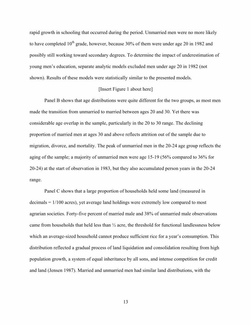
Figure 1 presents distributions of the primary predictors by respondent’s marital status for
each of the married and unmarried person-years in the analysis, starting with the respondent’s
individual resources (education and age). Panel A shows that about half of married and one-third
of unmarried respondents had completed no schooling. Only 8% of each group had completed
secondary school (10th), which is typically the minimum requirement for tenured government or
corporate employment. The higher proportion of unmarried men with any schooling reflects 4 Rural-rural moves, which typically involve individual seasonal migration episodes or nuclear family resettlement, require a separate analytic model that includes destination-specific resources that are relevant in the rural context (land purchase opportunities, local labor opportunities). International moves are difficult to model because income expectations depend more on labor relations and social connections than on education, and because international family migration is a rare event. 5 All models were also tested using a definition of family migration as a husband, wife, and children (if any were alive). Cases in which a husband and wife moved without their children were rare, and the models produced statistically similar results.
13
rapid growth in schooling that occurred during the period. Unmarried men were no more likely
to have completed 10th grade, however, because 30% of them were under age 20 in 1982 and
possibly still working toward secondary degrees. To determine the impact of underestimation of
young men’s education, separate analytic models excluded men under age 20 in 1982 (not
shown). Results of these models were statistically similar to the presented models.
[Insert Figure 1 about here]
Panel B shows that age distributions were quite different for the two groups, as most men
made the transition from unmarried to married between ages 20 and 30. Yet there was
considerable age overlap in the sample, particularly in the 20 to 30 range. The declining
proportion of married men at ages 30 and above reflects attrition out of the sample due to
migration, divorce, and mortality. The peak of unmarried men in the 20-24 age group reflects the
aging of the sample; a majority of unmarried men were age 15-19 (56% compared to 36% for
20-24) at the start of observation in 1983, but they also accumulated person years in the 20-24
range.
Panel C shows that a large proportion of households held some land (measured in
decimals = 1/100 acres), yet average land holdings were extremely low compared to most
agrarian societies. Forty-five percent of married male and 38% of unmarried male observations
came from households that held less than ½ acre, the threshold for functional landlessness below
which an average-sized household cannot produce sufficient rice for a year’s consumption. This
distribution reflected a gradual process of land liquidation and consolidation resulting from high
population growth, a system of equal inheritance by all sons, and intense competition for credit
and land (Jensen 1987). Married and unmarried men had similar land distributions, with the

14
exception of the higher proportion of married observations with no land holdings.6
The observation year distribution, shown in Panel D, was weighted toward earlier years
due to sample censoring. The unmarried sample was weighted toward early years as men shifted
into the married sample. Whereas the married sample gained observations in later years, this
growth did not make up for sample losses due to out-migration, divorce and mortality. The
sample showed no unexpected changes during the flood years of 1988 and 1989
The Great Flood of 1988 Extreme floods are the most devastating ecological crisis affecting inland areas such as Matlab,
destroying crops, altering the course of rivers, and permanently submerging land. The October
1988 flood in Bangladesh occurred at the end of the annual growing season, resulting not from
heavy rains, but from unusual flows of water from rivers draining the Himalayas. A majority of
permanent property loss was sustained by households living on river banks, where buildings and
land were inundated. Yet a broader segment of households suffered a more lasting set of indirect
effects, including disruptions in subsequent planting seasons, broken communications and
transport links, and commodity price distortions. A household’s ability to sustain the short-term
effects of a flood may be determined not merely by ecological factors, but also by a household’s
ability to manage risk and cope with crises.
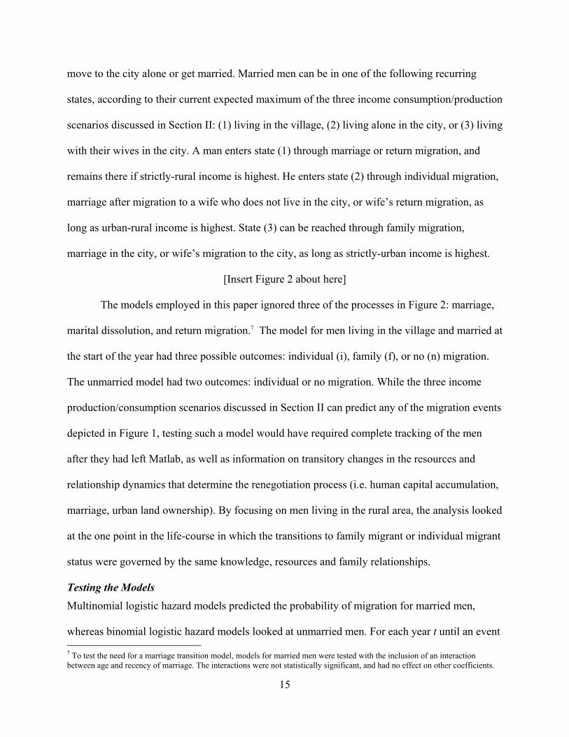
V. Estimating the Model Constructing a Static Model of Individual and Family Migration
Figure 2 depicts life-course migration and marriage decisions for men who reach adulthood
while living in the rural area. All men begin unmarried, after which, in any year, they can either
6 This may reflect a tendency toward earlier marriage among the landless (Barkat-e-Khuda 1987), but it also reflects differences in within-household land ownership. For unmarried men who live in their father’s households, household land holdings report fathers’ land. Married men are more likely to live in their own households, and may have yet to inherit parental land. One implication of this difference is that land estimates are a less perfect estimate of married men’s rural income. To test the impact of this effect, however, the models in Tables 1 and 2 were estimated separately for married men whose fathers had died; they were not statistically significant different from the general model.
15
move to the city alone or get married. Married men can be in one of the following recurring
states, according to their current expected maximum of the three income consumption/production
scenarios discussed in Section II: (1) living in the village, (2) living alone in the city, or (3) living
with their wives in the city. A man enters state (1) through marriage or return migration, and
remains there if strictly-rural income is highest. He enters state (2) through individual migration,
marriage after migration to a wife who does not live in the city, or wife’s return migration, as
long as urban-rural income is highest. State (3) can be reached through family migration,
marriage in the city, or wife’s migration to the city, as long as strictly-urban income is highest.
[Insert Figure 2 about here]
The models employed in this paper ignored three of the processes in Figure 2: marriage,
marital dissolution, and return migration.7 The model for men living in the village and married at
the start of the year had three possible outcomes: individual (i), family (f), or no (n) migration.
The unmarried model had two outcomes: individual or no migration. While the three income
production/consumption scenarios discussed in Section II can predict any of the migration events
depicted in Figure 1, testing such a model would have required complete tracking of the men
after they had left Matlab, as well as information on transitory changes in the resources and
relationship dynamics that determine the renegotiation process (i.e. human capital accumulation,
marriage, urban land ownership). By focusing on men living in the rural area, the analysis looked
at the one point in the life-course in which the transitions to family migrant or individual migrant
status were governed by the same knowledge, resources and family relationships.
Testing the Models Multinomial logistic hazard models predicted the probability of migration for married men,
whereas binomial logistic hazard models looked at unmarried men. For each year t until an event 7 To test the need for a marriage transition model, models for married men were tested with the inclusion of an interaction between age and recency of marriage. The interactions were not statistically significant, and had no effect on other coefficients.
16
occurred or a respondent was censored, the outcome for man k was, Mkt = j, j= i (individual), f
(family) or n (no) migration for married men and i (individual) or n (no) migration for unmarried
men.8 The general equation for both married and unmarried men fit a vector of predictive
coefficients X and a measure of time (t) according to the following equation:
∑=
∑
∑===
=
=
nfij
X
X
kt n
isksjs
n
isksjs
e
enfijjM
,,
),,,Pr(β
β
Because estimation could result in any number of solutions, no migration was chosen as a
reference event for which all values of 0=nβ . If there were no time dependencies (i.e., 0=jtβ )
or time dependencies were the same for all outcomes, the coefficient ijβ could be interpreted by
,)Pr()Pr(
ln iijn
j xMM
β=
the change in the log-odds of outcome j (relative to the reference event) due to a one-unit change
in the value of ix .
Models included village-level fixed-effects specified through controls for village of
origin.9 Fixed-effects were included to eliminate the impact of community-level factors such as
ecology and market development, and community-level variation in migration rates. Fixed-
effects models were statistically similar to those without fixed effects in terms of the joint
significance of any group of variables. This suggests that the individual- or household-level
heterogeneity of interest in the model was not simply the result of between-village differences.
8 Multinomial models must account for the “Independence of Irrelevant Alternatives” (IIA) assumption that the relative choice between outcomes 1 and 2 would not be affected by elimination of outcome 3. Hausmann specification tests compare coefficients and standard errors of possible two-outcome models with those of the chosen model. All tests show no significant differences between the two-outcome models and the chosen model (at the p<=0.01 level). 9 While estimating a fixed-effects multinomial logistic regression is problematic due to the categorical nature of the dependent variable, the inclusion of village-level controls in a standard model results in no bias as long as the number of observations per cell (village) approaches infinity. An average cell contains 1,800 married male person-years, and 600 unmarried ones.

17
Results are presented and interpreted through the use of Multiple Classification Analysis
(MCA) to account for the role of competing risks in multinomial models. Multinomial
coefficients and risk ratios do not bear a straightforward relationship to predicted probabilities, as
they do in binary models. For example, if a variable has a positive association with both family
and individual migration, then its true impact on the probability, say, of family migration
depends not only on the effect itself, but also on the reduced number of cases at risk because the
risk of individual migration has also increased. MCA calculates the predicted probability of each
outcome (family, individual or no migration) allowing the variable (or variables) or interest to
vary, while holding all other variables at their means (Retherford & Choe 1993):
∑=
+
+
∑+
∑===
≠
≠
nfij
XX
XX
rrjr
rssjs
rjrrs
sjs
e
enfijjM
,,1
),,,Pr(ββ
ββ
Results are primarily presented through two sets of graphical comparisons constructed from
MCA tables. The first compared predicted probabilities of any migration between unmarried and
married men. The probability of any migration for married men was calculated from the sum of
the probability of individual and family migration, which provided similar results to predictions
based on a binomial model of any migration for married men. The second broke predicted
probabilities of any migration for married men into their component parts: the predicted
probabilities of family and individual migration.
VI. Results Table 1 presents Model 1, which includes main effects for age, education, observation year and
household land holdings. All models include controls for village fixed effects, respondent’s
household headship status, household size and composition, religion, and whether the man’s
primary occupation is fisherman.
18
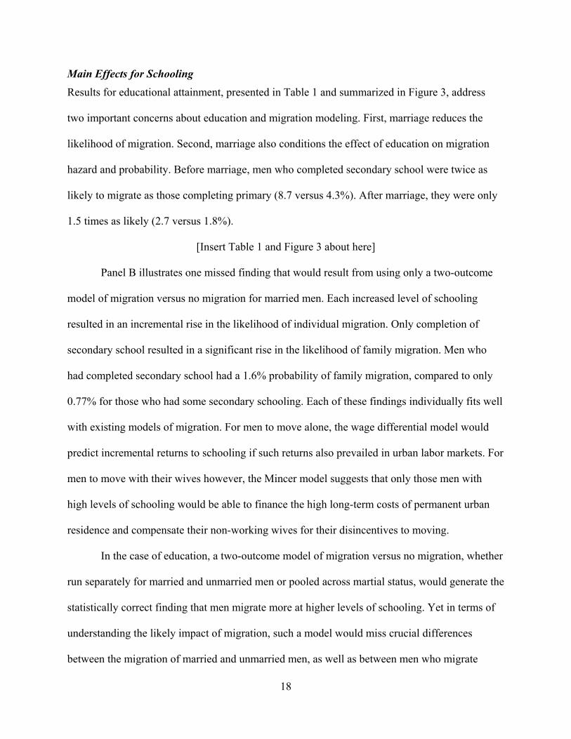
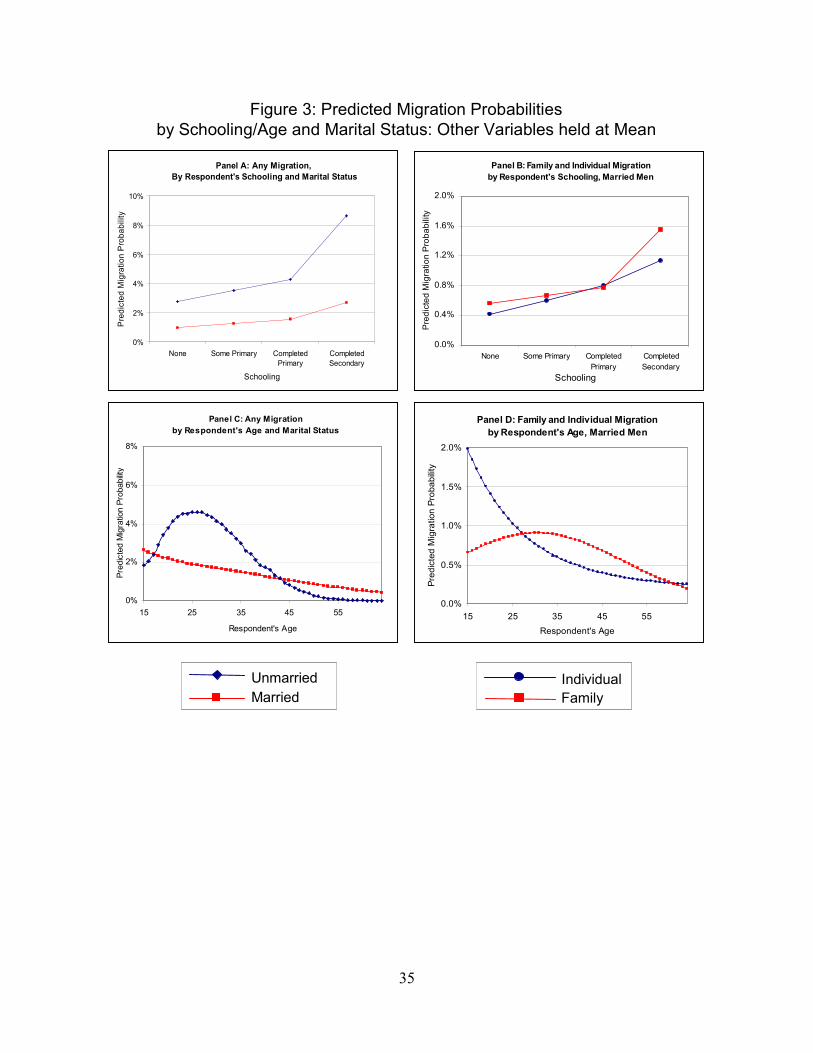
Main Effects for Schooling Results for educational attainment, presented in Table 1 and summarized in Figure 3, address
two important concerns about education and migration modeling. First, marriage reduces the
likelihood of migration. Second, marriage also conditions the effect of education on migration
hazard and probability. Before marriage, men who completed secondary school were twice as
likely to migrate as those completing primary (8.7 versus 4.3%). After marriage, they were only
1.5 times as likely (2.7 versus 1.8%).
[Insert Table 1 and Figure 3 about here]
Panel B illustrates one missed finding that would result from using only a two-outcome
model of migration versus no migration for married men. Each increased level of schooling
resulted in an incremental rise in the likelihood of individual migration. Only completion of
secondary school resulted in a significant rise in the likelihood of family migration. Men who
had completed secondary school had a 1.6% probability of family migration, compared to only
0.77% for those who had some secondary schooling. Each of these findings individually fits well
with existing models of migration. For men to move alone, the wage differential model would
predict incremental returns to schooling if such returns also prevailed in urban labor markets. For
men to move with their wives however, the Mincer model suggests that only those men with
high levels of schooling would be able to finance the high long-term costs of permanent urban
residence and compensate their non-working wives for their disincentives to moving.
In the case of education, a two-outcome model of migration versus no migration, whether
run separately for married and unmarried men or pooled across martial status, would generate the
statistically correct finding that men migrate more at higher levels of schooling. Yet in terms of
understanding the likely impact of migration, such a model would miss crucial differences
between the migration of married and unmarried men, as well as between men who migrate
19
alone and with their families.
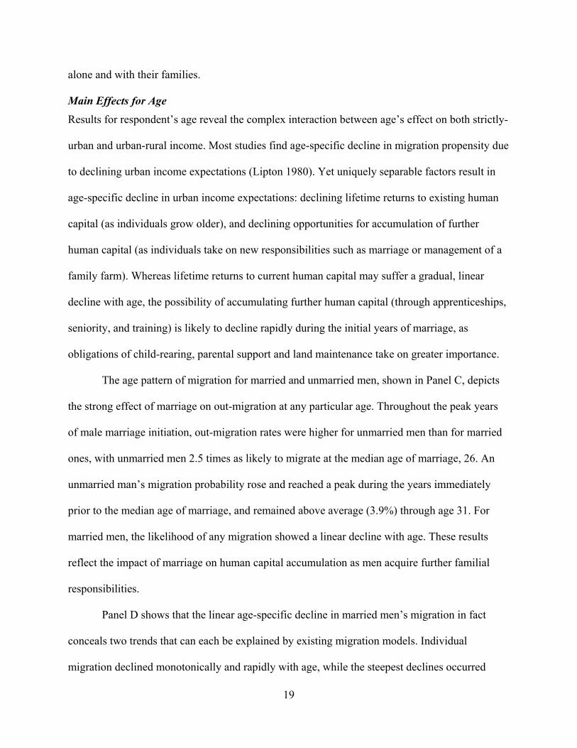
Main Effects for Age Results for respondent’s age reveal the complex interaction between age’s effect on both strictly-
urban and urban-rural income. Most studies find age-specific decline in migration propensity due
to declining urban income expectations (Lipton 1980). Yet uniquely separable factors result in
age-specific decline in urban income expectations: declining lifetime returns to existing human
capital (as individuals grow older), and declining opportunities for accumulation of further
human capital (as individuals take on new responsibilities such as marriage or management of a
family farm). Whereas lifetime returns to current human capital may suffer a gradual, linear
decline with age, the possibility of accumulating further human capital (through apprenticeships,
seniority, and training) is likely to decline rapidly during the initial years of marriage, as
obligations of child-rearing, parental support and land maintenance take on greater importance.
The age pattern of migration for married and unmarried men, shown in Panel C, depicts
the strong effect of marriage on out-migration at any particular age. Throughout the peak years
of male marriage initiation, out-migration rates were higher for unmarried men than for married
ones, with unmarried men 2.5 times as likely to migrate at the median age of marriage, 26. An
unmarried man’s migration probability rose and reached a peak during the years immediately
prior to the median age of marriage, and remained above average (3.9%) through age 31. For
married men, the likelihood of any migration showed a linear decline with age. These results
reflect the impact of marriage on human capital accumulation as men acquire further familial
responsibilities.
Panel D shows that the linear age-specific decline in married men’s migration in fact
conceals two trends that can each be explained by existing migration models. Individual
migration declined monotonically and rapidly with age, while the steepest declines occurred
20
prior to age 30. This result may reflect not merely the process of declining returns to human
capital outlined by the WD model, but also a rapid reduction in the long-term benefits of short-
term circular migration episodes suggested by the NE model.
In contrast, family migration initially rose with age, resulting in a peak at age 31; it
remained the more likely of the two migration outcomes at each age after 27. A number of life
course changes may explain this pattern, which can be split into two questions: 1) why does the
likelihood of family migration not decrease as rapidly as individual migration, and 2) why does
the likelihood of family migration increase?
Likely explanations lay in the typical age pattern of rural income expectations in
Bangladesh. First, rural income expectations may decline if households tend to liquidate land
following the initial 1982 baseline (Jahangir 1979). Second, expected urban-rural income
opportunities may decline over the life courses as a man’s own individual migration
opportunities diminish, as between-sibling cooperation declines, and as elderly parents provide
less labor and require greater support and assistance (Jensen 1987). Research on household
economic life cycles has shown that the period of greatest economic vulnerability occurs when
adults are in early middle age, after their own economic opportunities have diminished, yet
before children are old enough to enter the labor market themselves. After looking at the impact
of rural resources on migration, we revisit this issue by looking at the age-pattern of migration in
1989, the year immediately following a major flood.
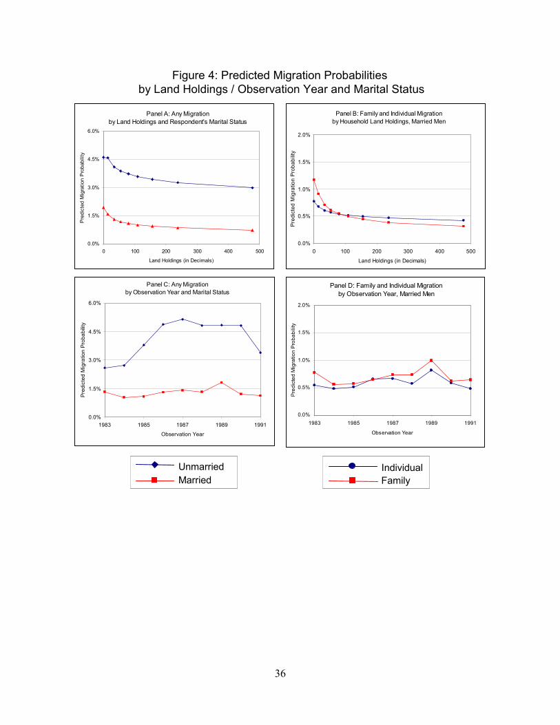
Main Effects for Household Land Holdings Household land holdings have been found to be a key determinant of rural-urban migration in
most settings, and typically individuals are more likely to move if their households own less
land. Yet WD and NE models offer different explanations for this effect, and slightly different
expectations. As the principal determinant of income in most rural settings, WD expects a

21
monotonic negative relationship; more land holdings lead to less income, and thus, other things
being equal, a greater likelihood of migration. NE explains the role of land not just in terms of
income, but in terms of a need for investment capital and insurance against the risks of
agricultural production. Households with large land holdings are better placed to self-insure,
either through crop diversification or other non-agricultural assets, and their members should be
less likely to migrate. Households with no land holdings should be less directly exposed to the
risks of agricultural production, and able to diversify their labor activities into agricultural and
non-agricultural activities; while they may be poorer than households with small land holdings,
their members may also have less reason to migrate.
Two land measures are therefore estimated: an indicator of whether any land was held by
the household and the log of total household land holdings (set to zero for no land). This model
further offered the best fit of all categorical, linear or logged land specifications. Logged land
holdings had a negative association with all forms of migration (Table 1), but a stronger
association with family migration (-0.318 coefficient) than with individual migration by married
(-0.135) or unmarried men (-0.146). For married men, any household land ownership had a
further negative association with family moves, but no significant association with individual
ones. No land ownership effect was found for unmarried men.
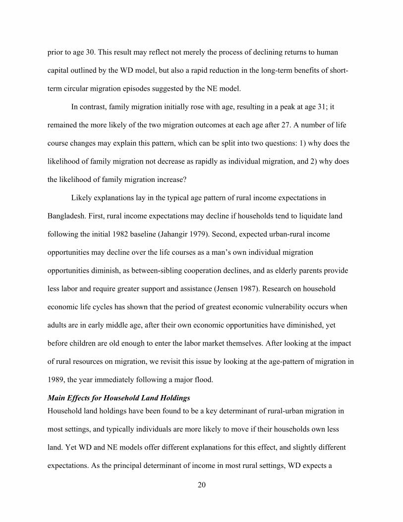
The relationship between land holdings and migration assuming a two-outcome model
are depicted for married and unmarried men in Figure 4, Panel A. Under the two-outcome model,
the likelihood of migration would experience a monotonic, asymptotic decline with increasing
land holdings, with the steepest part of the curve affecting households with 100 decimals of land
or less. Unmarried men would have a 4.6% likelihood of moving out of a landless household,
compared to 3.3% from a household with 100 decimals, while married men’s migration
22
likelihood would decline from 2.0% to 1.0%.
[Insert Figure 4 about here]
Yet Figure 4, Panel B shows that land’s effect on migration depends greatly on the choice
of family or individual migration. Family migration was considerably more likely among men
from landless households (1.2% versus 0.8%). The likelihood of both forms of migration drops
with greater land holdings, yet family migration experiences a much steeper decline (four times
more likely among the landless compared to the top land holding decile, whereas individual
moves were only twice as likely). What results is a crossover: family migration was more likely
among men from households holding less than 100 decimals of land, while individual moves
were preferred among those with more. The individual migration effect offers some support for
both WD and NE models of migration; individuals are encouraged to migrate alone if their
households have small land holdings, indicating a low income, yet perhaps some prospect of
investing migrant earnings into increased production. The family migration effect suggests that
when a man is considering whether to move with his nuclear family, income is of paramount
concern.
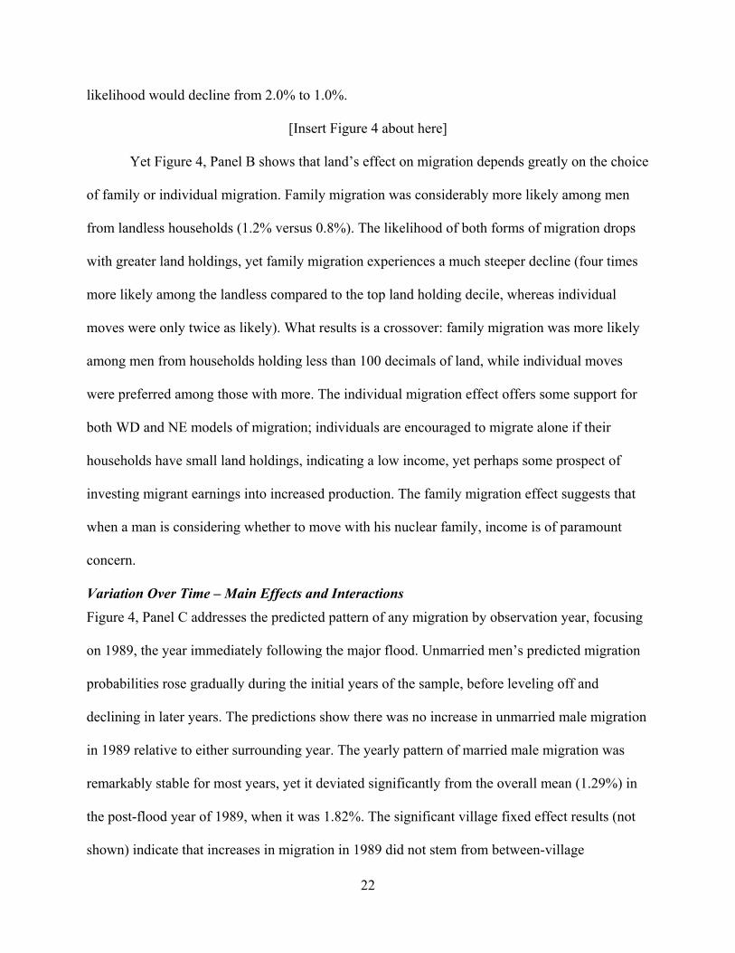
Variation Over Time – Main Effects and Interactions Figure 4, Panel C addresses the predicted pattern of any migration by observation year, focusing
on 1989, the year immediately following the major flood. Unmarried men’s predicted migration
probabilities rose gradually during the initial years of the sample, before leveling off and
declining in later years. The predictions show there was no increase in unmarried male migration
in 1989 relative to either surrounding year. The yearly pattern of married male migration was
remarkably stable for most years, yet it deviated significantly from the overall mean (1.29%) in
the post-flood year of 1989, when it was 1.82%. The significant village fixed effect results (not
shown) indicate that increases in migration in 1989 did not stem from between-village
23
differences such as proximity to a river or flood-control facilities.
WD and NE models both offer insight into the mechanisms linking a major flood to
increasing migration, and each explanation relates further to the role of household land
resources. According to WD, a decline in income, perhaps permanent, might raise the
attractiveness of urban areas relative to the affected rural area. For households already lacking in
land holdings, these effects might be particularly important. According to NE, short-term
migration opportunities might allow households to mitigate the short-term effects of the flood
with an infusion of remittance income. Yet again, factors that allow households to use migration
as a means of mitigating future risks might also be better placed to use migration to alleviate an
ongoing crisis.
To address this issue, Model 2 (Table 2) contains observation-year interactions with
household landlessness. Log-likelihood statistics in Table 2 show the statistical importance of the
included interactions, which reduced the predicted underestimate of migration (family migration
in particular) in 1989 (not shown). Interactions between logged land holdings and observation
year did not significantly improve model fit.
[Insert Table 2 about here]
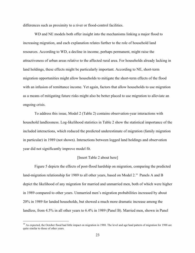
Figure 5 depicts the effects of post-flood hardship on migration, comparing the predicted
land-migration relationship for 1989 to all other years, based on Model 2.10 Panels A and B
depict the likelihood of any migration for married and unmarried men, both of which were higher
in 1989 compared to other years. Unmarried men’s migration probabilities increased by about
20% in 1989 for landed households, but showed a much more dramatic increase among the
landless, from 4.5% in all other years to 6.4% in 1989 (Panel B). Married men, shown in Panel
10 As expected, the October flood had little impact on migration in 1988. The level and age/land pattern of migration for 1988 are quite similar to those of other years.
24
B, were 40% more likely to migrate in 1989 than in other years. Using only the two-outcome
approach, the difference between 1989 and other years was only slightly higher for men from
landless households, who were 50% more likely to move in 1989.
[Insert Figure 5 about here]
Based solely on Panel B, it would appear that migration grows more likely to an equal
extent among households across the land distribution, and thus that household land holdings do
not mediate the use of migration to respond to an economic crisis. Yet Panels C and D reveal
that, as with the likelihood of migration in a typical year, household land holdings determine
whether the increased likelihood of migration is reflected in individual or family moves. For men
from landed households, the probability of individual migration (shown in Panel C) rose by 30%
in 1989 relative to other years combined, compared to only 16% among men from landless
households. Controlling for other factors, the likelihood of family migration (shown in Panel D)
sustained a much sharper increase in 1989, 55%, compared to 27% increase in the likelihood of
individual migration. Furthermore, this increase occurred disproportionately among men from
landless households, who were 80% more likely to move with their families in 1989 (2.0%
compared to 1.1%), than among men from landed households (47% more likely).
VII. Conclusion: A Note on Migration Theory and Policy The results of this paper offer further evidence that the concerns of the two prevailing
microeconomic models of migration, the Wage Differential and New Economic Models, may
both be relevant in the same setting. Yet by incorporating a three-outcome model of migration,
they also suggest not so much a diversity of motivations as heterogeneity in terms of the practice
of migration and the individuals practicing it. Determinants of individual migration are
suggestive both of the income deficits hypothesized by the Wage Differential Model and the
household economic diversification hypothesis of the New Economic Model. Family migration
25
responds more strictly to the concerns of the Wage Differential Model.
A number of specific differences in the determinants of family and individual migration
would be missed were a simple two-outcome model employed. Individual migration is more
likely among those with small land holdings, while family migration is more likely among those
with no land holdings. Following marriage, the likelihood of individual migration declines
rapidly, while the likelihood of family migration rises for several years following the mean age
of marriage. Most importantly, in the aftermath of the major 1988 flood, increasing family
migration accounted for most the substantial increase in the likelihood of migration in 1989.
Furthermore, a two-outcome model would suggest that the 1989 migration increase occurred
across the land distribution, when in fact the increase in family migration occurred
disproportionately among men from landless households.
These results carry both direct and indirect implications for our understanding of the
effects of rural-urban migration on future demographic and sociological trends in a rapidly
urbanizing society such as Bangladesh. For urban migrant-receiving areas, compositional
differences between family and individual migrants are of paramount importance. Past research
has shown that migrant families are more likely than individual movers to settle in slums or
squatter settlements, while asserting that migrating families are likely to be less suited to the
urban economy and less able to fall back on rural family or resources for support or return
migration. This work confirms the latter assertion, showing that family migrants may be older
and come from rural households with fewer land holdings than individual migrants. As a result,
it is likely in particular that those women and children who move to the city are selected from the
lowest rural socioeconomic strata. While LDC cities anticipate massive migrant inflows
following major rural catastrophes such as floods, these results suggest that they should also

26
expect those migrants to move with families, and to be even more strongly selected from the
lowest rural socioeconomic strata.
From the standpoint of rural migrant-sending areas, these results extend research on the
role of resource deprivation in hastening the fission of households and limiting subsequent
interhousehold cooperation to the sphere of interregional social networks. For rural elders in
particular, family migration may reduce the likelihood and value of migrant remittances and
deprive them of the benefits of joint coresidence with daughters-in-law and grandchildren (e.g.
jointly consuming migrant remittances, receiving labor and care). The results suggest that such
an outcome is most likely to affect those with limited land resources, particularly in the year
following a major ecological and economic crisis. Households with sufficient land resources, on
the other hand, appear well-placed to take advantage of the opportunities afforded by individual
migration.
From a stratification and development perspective, the divergence in age- and land-
specific migration patterns would not be a problem were the expected outcomes of family and
individual migration reasonably similar. Yet research in this context and others has shown that
this is not the case (Root & De Jong 1992; Perlman 1976). Family migration is a process that is
not taken lightly: it is costly, typically involves residence in slums, and is often irreversible
(Kuhn 1999). Family migration not only separates the movers from their traditional base of
security, but it also separates stayers from their most dynamic source of economic support. In the
case of the elderly, family migration often removes a primary source of financial support and
labor (a son) as well as a primary source of personal care (a daughter-in-law). From a parent’s
perspective, family migration is akin to losing a son; individual migration is akin to gaining an
income source. In the long run, the results raise further concerns about a disincentive to invest in
27
children; if landless households can expect more limited support from their out-migrant children,
they may find less incentive to invest in children’s education.
This research raises a call for the development of a more synthetic migration theory, and
more innovative tests of the meaning, context, and likely impact of migration. While the specific
causes and uses of migration from rural Bangladesh are unique to its ecosystem and economic
structure, the patterns have general applicability to almost any migrant-sending region, to
internal and international migration, to men’s and women’s migration, and to forced and
voluntary migration. In all cases, migrant outcomes that are considered unique to the context
may in part be explained by a migrant’s desire and ability to maintain strong social and
economic linkages with members of the origin community. There is now a mountain of evidence
explaining why migrants leave home and even more evidence explaining why they never really
leave home, yet we have only begun to ask what allows them to do both.
References Afsar, R. (1994). “Internal Migration and Women: An Insight into Causes, Consequences, and
Policy Implications.” The Bangladesh Development Studies 2 & 3: 217-243. Amin, S., Diamond, I. Naved, R.T., & Newby, M. (1998). “Transition to Adulthood of Female
Garment-Factory Workers in Bangladesh.” Studies in Family Planning 29: 185-200. Becker, G.S. 1974. “A Theory of Social Interactions.” Journal of Political Economy 82
(November/December). no. 6: 1063-94. Chen, L.C., Chowdhury, A.K.M.A. & Huffman, S.L. (1979). Seasonal Dimensions of Energy
Protein Malnutrition in Rural Bangladesh: The Role of Agriculture, Dietary Practices, and Infection. Ecology of Food and Nutrition, 8: 175-187.
Connell, J., Dasgupta, B., Laishley, R. & Lipton, M. (1976). Migration from Rural Areas: The
Evidence from Village Studies. Delhi. Oxford University Press. de Haan, A. (1999). “Livelihoods and Poverty: The Role of Migration – A Cricial Review of the
Migration Literature”. The Journal of Development Studies 36: 1-47. de Haan, A. & Rogaly, B. (2002). “Introduction: Migrant Workers and Their Role in Rural
Change”. Journal of Development Studies, Special Issue on Labour Mobility and Rural Society 38 (5): 1-14.
de Janvry, A. & Garramon, C. (1977). "The Dynamics of Rural Poverty in Latin America".
Journal of Peasant Studies 5(2):206-216. Durand, J., Kandel, W., Parrado, E.A. & Massey, D.S. (1996, May). “International Migration
and Development in Mexican Communities”. Demography 33(2):249-64. Ellis, F. (1998). “Households Livelihood Strategies and Rural Livelihood Diversification”. The
Journal of Development Studies 35: 1-38. Faist, T. (2000). The Volume and Dynamics of International Migration and Transnational Social Spaces. New York: Clarendon Press. Fauveau, V. (Ed.) (1994). Matlab: Women, Children and Health. Dhaka, Bangladesh: ICDDR,B Frankenberg, E. & Kuhn, R. (2001). “Old Age Support from Sons and Daughters: Bangladesh
and Indonesia in Comparison.” Paper presented at the Annual Meeting of the Population Association of America, Washington, DC.
Gardner, K. 1995. Global migrants, local lives: Travel and transformation in rural Bangladesh.
Oxford: Clarendon Press. Gereffi, G. & Korzeniewicz, M., ed. (1994). Commodity Chains and Global Capitalism.
29
Westport, CT: Greenwood Press. Harris, J.R. & Todaro, M.P. (1970). “Migration, Unemployment and Development: A Two
Sector Analysis”. American Economic Review 60(1):126-142. Jahangir, B.K. (1979). Differentiation Polarization and Confrontation in Rural Bangladesh.
Center for Social Studies, University of Dhaka. Jensen, E.G. (1987). Rural Bangladesh: Competition for Scarce Resources. Dhaka, Bangladesh:
University Press Limited. Kanaiaupuni S.M. & Donato, K.M. (1999). “Migradollars and mortality: The effects of migration
on infant survival in Mexico”. Demography 36(3): 339-353. Kuhn, R. (1999). The Logic of Letting Go: Family and Individual Migration from Rural
Bangladesh. Unpublished Doctoral Thesis. Philadelphia: University of Pennsylvania. Kuhn, R. (2000a). Understanding the Social Process of Rural-Urban Migration in Bangladesh.
Unpublished manuscript. Kuhn, R. (2000b). “Elderly Remittances and Urban-Rural Security Relationships in
Bangladesh”. Paper Presented to Conference on Thinking Longitudinally: Issues in the Design and Analysis of Panel Data for Aging Research, February 25, 2000: Singapore.
Lewis, W.A. (1954). Economic Development with Unlimited Supplies of Labor. The Manchester
School of Economic and Social Studies 22:139-191. Lipton, M. (1980). Migration from Rural Areas of Poor Countries: The Impact and on Rural
Productivity and Income Distribution. World Development 8:1-24. Lomnitz, Larissa (1977). Networks and Marginality: Life in a Mexican Shantytown. New York:
Academic Press. Lucas, R.E B. & Stark, O. (1985, October). Motivations to Remit: Evidence from Botswana.
Journal of Political Economy 93:901-18. Massey, D.S. & Parrado, E.A. (1994). Migradollars: The Remittances and Savings of Mexican
Migrants to the United States. Population Research and Policy Review. 13:3-30. Massey, D.S. & Espinosa, K. (1997). What’s Driving Mexico-US Migration: A Theoretical,
Empirical and Policy Analysis. American Journal of Sociology 102:939-999. Massey, D.S., Arango, J., Hugo, G., Kouaouci, A., Pellegrino, A. & Taylor, J.E. (1999). Worlds
in Motion: Understanding International Migration at The End of The Millennium. New York: Oxford University Press.
30
Mincer, J. (1978). Family Migration Decisions. Journal of Political Economy. 8(2):749-773. Nabi, A.K.M.N. (1992). Dynamics of Internal Migration in Bangladesh. Canadian Studies in
Population 19(1):81-98. Perlman, J.E. (1976). The Myth of Marginality: Urban Poverty and Politics in Rio de Janeiro.
Berkeley: University of California Press. Ranis, G. & Fei, J.C.H. (1961). A Theory of Economic Development. American Economic
Review 51:533-565. Retherford, R.D. & Choe, M.K. (1993). Statistical Models for Causal Analysis. New York: John
Wiley and Sons. Root, B.D. & De Jong, G.F. (1991). “Family Migration in a Developing Country”. Population
Studies 45(2): 221-233. Rosenzweig, M.R. & Stark, O. (1989). “Consumption Smoothing, Migration, and Marriage.”
Journal of Political Economy 97: 905-26. Roy, K.C., Tisdell, C. & Alauddin, M. (1992). Rural-Urban Migration and Poverty in South
Asia. Journal of Contemporary Asia 22(1):57-72. Shaw, A. (1988, January). The Income Security Function of the Rural Sector: The Case of
Calcutta, India. Economic Development and Cultural Change 36:303-14. Sjaastad, L.A. (1962). The Costs and Returns of Human Migration. Journal of Political Economy
70:80-93 Stark, O. (1982). Research on Rural-to-Urban Migration in LDCs: The Confusion Frontier and
Why We Should Pause to Rethink Afresh. World Development 10(1):63-70. Stark, O. & Katz, E. (1986). “Labor Migration and Risk Aversion in Less Developed Countries”.
Journal of Labor Economics 4:134-149. Taylor, J.E. & Wyatt, T. J. (1996). The Shadow Value of Migrant Remittances, Income and
Inequality in a Household-farm Economy. The Journal of Development Studies 32:899-912. Todaro, M.P. (1969). A Model of Labor Migration and Urban Unemployment in Less-Developed
Countries. The American Economic Review 59:138-148. Unnithan-Kumar, M. 2003. Spirits of the womb: Migration, motherhood and healthcare in
Rajasthan. Contributions to Indian sociology. 37(1&2): 163-187. VanWey, L.K. (2003). “Land Ownership as a Determinant of Temporary Migration in Nang
Rong, Thailand.” European Journal of Population 19: 121-145.
31
Notes: * p<=0.05; ** p<=0.01; *** p <= .001. Model includes controls for village fixed effects, respondent’s household headship status, household size and composition, religion, and whether occupation is fisherman.
Table 1: Results of Fixed Effects Logistic Models of Migration, Adult Males in Matlab (1983-1991) Model 1: Main Effects Only
Married Men Unmarried Men
Individual Family Individual
Coefficient S.E. Coefficient S.E. Coefficient S.E.
Education (1-4) 0.452*** 0.072 0.198*** 0.066 0.300*** 0.053 Education (5-9) 0.816*** 0.070 0.420*** 0.066 0.662*** 0.049 Education (10+) 1.127*** 0.093 1.181*** 0.079 1.372*** 0.073 Year = 1984 -0.117 0.110 -0.316*** 0.102 0.053 0.070 Year = 1985 -0.051 0.110 -0.280*** 0.102 0.412*** 0.068 Year = 1986 0.204* 0.105 -0.155 0.099 0.682*** 0.069 Year = 1987 0.230** 0.106 -0.012 0.097 0.746*** 0.073 Year = 1988 0.090 0.112 -0.001 0.098 0.687*** 0.079 Year = 1989 0.453*** 0.106 0.309*** 0.093 0.701*** 0.085 Year = 1990 0.112 0.116 -0.159 0.105 0.707*** 0.092 Year = 1991 -0.087 0.126 -0.134 0.107 0.355*** 0.110 Age -0.099*** 0.018 0.078*** 0.019 0.222*** 0.039 Age-Squared 0.001*** 0.000 -0.001*** 0.000 -0.004*** 0.001 Household Has Any Land -0.069 0.085 -0.117* 0.061 0.091 0.069 Log Household Land -0.135*** 0.030 -0.318*** 0.029 -0.146*** 0.020 Constant -1.792*** 0.399 -5.545*** 0.436 -6.118***
0.490
Dependent Variable Mean 0.0059 0.0070 0.0387
Observations 264,184 90,579
Log Likelihood R^2 (DF) 2988.3 (342) 1589.5 (171)

32
Note: Coefficients followed by 3, 2, and 1 stars are significantly different from zero at the 1, 5, and 10 percent level, respectively. Model includes controls for village fixed effects, respondent’s household headship status, household size and composition, religion, and whether occupation is fisherman.
Table 2: Results of Fixed Effects Logistic Models of Migration, Adult Males in Matlab (1983-1991) Model 2: Main Effects and Observation Year Interactions with Age, Land
Married Men Unmarried Men Individual Family Individual Coefficient S.E. Coefficient S.E. Coefficient S.E. Education (1-4) 0.447*** 0.072 0.197*** 0.066 0.297*** 0.053 Education (5-9) 0.818*** 0.070 0.423*** 0.066 0.669*** 0.050 Education (10+) 1.172*** 0.093 1.208*** 0.080 1.363*** 0.074 Year = 1984 0.129 0.344 -0.109 0.376 -0.404 0.409 Year = 1985 0.208 0.340 -0.067 0.373 0.547 0.409 Year = 1986 0.431 0.326 0.373 0.363 1.038** 0.420 Year = 1987 0.770** 0.334 0.181 0.353 1.170** 0.457 Year = 1988 1.183*** 0.366 1.057*** 0.361 2.090*** 0.534 Year = 1989 1.724*** 0.344 0.392 0.341 1.496** 0.592 Year = 1990 1.215*** 0.385 1.335*** 0.398 1.281* 0.667 Year = 1991 1.360*** 0.440 1.197*** 0.405 2.802*** 0.951 Age -0.089*** 0.020 0.082*** 0.019 0.175*** 0.039 Age-Squared 0.001*** 0.000 -0.001*** 0.000 -0.004*** 0.001 Household Has Any Land -0.300* 0.178 -0.505*** 0.143 -0.176 0.139 Log Household Land 0.095 0.069 -0.161** 0.074 -0.283*** 0.095 Age * Log Household Land -0.007*** 0.002 -0.004** 0.002 0.006 0.004 Age * Year = 1984 -0.007 0.010 -0.003 0.010 0.022 0.019 Age * Year = 1985 -0.005 0.010 -0.002 0.010 -0.004 0.019 Age * Year = 1986 -0.004 0.009 -0.007 0.010 -0.014 0.019 Age * Year = 1987 -0.015 0.009 0.001 0.009 -0.016 0.020 Age * Year = 1988 -0.030*** 0.011 -0.023** 0.010 -0.059** 0.023 Age * Year = 1989 -0.036*** 0.010 0.000 0.009 -0.032 0.025 Age * Year = 1990 -0.031*** 0.011 -0.037*** 0.011 -0.022 0.027 Age * Year = 1991 -0.042*** 0.013 -0.033*** 0.011 -0.094** 0.038 Any Land * Year = 1984 0.058 0.248 0.208 0.208 0.062 0.190 Any Land * Year = 1985 0.378 0.258 0.371* 0.210 0.454** 0.194 Any Land * Year = 1986 0.373 0.243 0.760*** 0.212 0.365* 0.188 Any Land * Year = 1987 0.196 0.238 0.612*** 0.201 0.474** 0.201 Any Land * Year = 1988 0.357 0.257 0.710*** 0.204 0.221 0.207 Any Land * Year = 1989 0.322 0.236 0.197 0.182 0.203 0.225 Any Land * Year = 1990 0.229 0.258 0.494** 0.212 0.564** 0.268 Any Land * Year = 1991 0.099 0.275 0.294 0.207 0.456 0.320 Constant -2.467*** 0.456 -6.039*** 0.485 -5.605*** 0.522 Dependent Variable Mean 0.0059 0.0070 0.0387 Observations 264,184 90,579 Log Likelihood R^2 3099.5 (376) 1624.6 (188) Joint Log-Likelihood Tests: Landless/Year Interactions 32.1 (16)*** 11.8 (8) Age/Year Interactions 62.9 (16)*** 15.9 (8)**

33
Figure 1: Distributions of Predictor VariablesAccording to Marital Status: Males Aged 15-65
MarriedUnmarriedMarriedUnmarried
Panel A: Educational Attainment
0%
15%
30%
45%
60%
0 1-4 5-9 10+
Years of Schooling
Per
cent
age
Panel B: Respondent's Age
0%
15%
30%
45%
60%
15-19 25-29 35-39 45-49 55-59Age Group
Per
cent
age
Panel C: Household Land Holdings
0%
6%
12%
18%
24%
0 100 200 300 400 500Decimals of Land
Per
cent
age
Panel D: Observation Year
0%
3%
6%
9%
12%
15%
1983 1985 1987 1989 1991Year
Perc
enta
ge
34
Unmarried, In Village
Married,In Village (1)
Unmarried,Alone in City
Married, Alone in City (2)
Individual Migration
Marriage/
Divorce
Marriage
Individual Migration
Married,Family in City (3)
Urban marriage
Wife’s Migration
Family Migration
Figure 2: Schema of Dynamic Model of Family and Individual Migration
35
Figure 3: Predicted Migration Probabilities by Schooling/Age and Marital Status: Other Variables held at Mean
Panel B: Family and Individual Migrationby Respondent's Schooling, Married Men
0.0%
0.4%
0.8%
1.2%
1.6%
2.0%
None Some Primary CompletedPrimary
CompletedSecondary
Schooling
Pre
dict
ed M
igra
tion
Pro
babi
lity
Panel A: Any Migration, By Respondent's Schooling and Marital Status
0%
2%
4%
6%
8%
10%
None Some Primary CompletedPrimary
CompletedSecondary
Schooling
Pre
dict
ed M
igra
tion
Pro
babi
lity
Panel D: Family and Individual Migration by Respondent's Age, Married Men
0.0%
0.5%
1.0%
1.5%
2.0%
15 25 35 45 55Respondent's Age
Pred
icte
d M
igra
tion
Prob
abilit
yPanel C: Any Migration
by Respondent's Age and Marital Status
0%
2%
4%
6%
8%
15 25 35 45 55
Respondent's Age
Pred
icte
d M
igra
tion
Prob
abilit
y
MarriedUnmarriedMarriedUnmarried Individual
FamilyIndividualFamily
36
Figure 4: Predicted Migration Probabilities by Land Holdings / Observation Year and Marital Status
MarriedUnmarriedMarriedUnmarried Individual
FamilyIndividualFamily
Panel D: Family and Individual Migration by Observation Year, Married Men
0.0%
0.5%
1.0%
1.5%
2.0%
1983 1985 1987 1989 1991
Observation Year
Pre
dict
ed M
igra
tion
Pro
babi
lity
Panel C: Any Migration by Observation Year and Marital Status
0.0%
1.5%
3.0%
4.5%
6.0%
1983 1985 1987 1989 1991
Observation Year
Pred
icte
d M
igra
tion
Prob
abilit
y
Panel B: Family and Individual Migration by Household Land Holdings, Married Men
0.0%
0.5%
1.0%
1.5%
2.0%
0 100 200 300 400 500
Land Holdings (in Decimals)
Pred
icte
d M
igra
tion
Prob
abilit
y
Panel A: Any Migration by Land Holdings and Respondent's Marital Status
0.0%
1.5%
3.0%
4.5%
6.0%
0 100 200 300 400 500
Land Holdings (in Decimals)
Pre
dict
ed M
igra
tion
Pro
babi
lity

37
1989All Other Years1989All Other Years
Figure 5: Predicted Migration Probabilitiesby Household Land Holdings, 1989 vs. All Other Years Combined
Panel C: Individual Migration by Married Men1989 vs. All Other Years
0.0%
0.3%
0.6%
0.9%
1.2%
1.5%
0 100 200 300 400 500Land Holdings (in Decimals)
Mig
ratio
n P
roba
bilit
y
Panel B: Any Migration by Married Men1989 vs. All Other Years
0%
1%
1%
2%
2%
3%
0 100 200 300 400 500Land Holdings (in Decimals)
Mig
ratio
n P
roba
bilit
yPanel D: Family Migration by Married Men
1989 vs. All Other Years
0.0%
0.5%
1.0%
1.5%
2.0%
2.5%
0 100 200 300 400 500
Land Holdings (in Decimals)
Mig
ratio
n Pr
obab
ility
Panel A: Any Migration by Unmarried Men1989 vs. All Other Years
0.0%
1.5%
3.0%
4.5%
6.0%
7.5%
0 100 200 300 400 500Land Holdings (in Decimals)
Mig
ratio
n P
roba
bilit
y
1989All Other Years1989All Other Years