The design, deployment and testing of Kriging models in GEOframeMarialaura Bancheri1, Francesco Serafin1, Michele Bottazzi1, Wuletawu Abera3, Giuseppe Formetta2,and Riccardo Rigon1

1 Department of Civil, Environmental and Mechanical Engineering, University of Trento, Italy2 Centre for Ecology & Hydrology, Crowmarsh Gifford, Wallingford, UK3 International Center for Tropical Agriculture (CIAT), P.O.BOX 5689, Addis Ababa, Ethiopia

Correspondence to: Marialaura Bancheri (marialaura.bancheri@unitn.it)

Abstract. This work presents a software package for the interpolation of climatological variables, such as temperature and

precipitation, using Kriging techniques. The purposes of the paper are: (1) to present a geostatistical software that is easy to

use and easy to plug-in to a hydrological model; (2) to provide a practical example of an accurately designed software from

the perspective of reproducible research; and (3) to demonstrate the goodness of the results of the software and so have a

reliable alternative to other, more traditional tools. Eleven types of theoretical semivariograms and four types of Kriging were5

implemented and gathered into Object Modelling System compliant components. The package provides real time optimization

for semivariogram and kriging parameters. The software was tested using a year’s worth of hourly temperature readings and a

rain storm event (11h) recorded in 2008 and retrieved from 97 meteorological stations in the Isarco River basin, Italy. For both

the variables, good interpolation results were obtained and then compared to the results from the R package, gstat.

1 Introduction10

Meteorological forcing data such as rainfall, temperature, and solar radiation are the dominant controlling factors for the hy-

drological cycle, energy balance and ecosystem processes (Ly et al., 2013). These data, besides being important of themselves,

are the natural input to distributed and semi-distributed hydrological models. Their quality and precision affect the accuracy

of results, (Xu and Singh, 1998; Stooksbury et al., 1999; Balme et al., 2006; Abera et al., 2017). In fact, all the surface water

models require a reliable precipitation dataset that is complete both in space and in time. Quite often, however, datasets of15

hydrological variables suffer from errors and missing data, therefore, filling the gaps in time series by estimating the missing

values is a common approach to solving this problem, (Eischeid et al., 2000; Saghafian and Bondarabadi, 2008; Di Piazza

et al., 2011; Adhikary et al., 2015). Several algorithms for the spatial interpolation of meteorological data are available in the

literature: Thiessen polygons (e.g., Thiessen, 1911; WMO, 1994), inverse distance methods (Ly et al., 2013), interpolation with

splines (e.g., Mitášová and Mitáš, 1993; Hutchinson, 1995), Kriging (e.g., Krige, 1951; Matheron, 1981; Goovaerts, 1997) and20

other types of interpolation (e.g., Robeson, 1992; Li and Heap, 2011, and references therein). Their performances have been

assessed by several authors, among others Tabios and Salas (1985) and Jarvis and Stuart (2001), who have concluded that

Kriging is one of the best techniques for the spatial interpolation of climatological variables. More specifically, Creutin and

1

Obled (1982) and Tabios and Salas (1985) demonstrated that for monthly rainfall and storm totals it is preferable to other

rainfall interpolation methods. Goovaerts (2000), Lloyd (2005), Basistha et al. (2008), Ly et al. (2011) confirmed these results.

Generally, Kriging can be applied to a wide range of datasets (e.g., Stahl et al., 2006; Phillips et al., 1992), and allows

for the estimation of the variance of interpolated quantities (e.g., Li and Heap, 2011). The interpolation can be improved

with the use of auxiliary variables, such as terrain-related parameters (e.g., relief, slope and aspect), as investigated in Attorre5

et al. (2007). Not surprisingly, Carrera-Hernández and Gaskin (2007) found that the use of elevation as a secondary variable

improves temperature prediction.

However, Kriging can be computationally more demanding than other interpolation techniques. To overcome this problem,

most applications that implement Kriging interpolators use either long time series with long time-steps, such as daily, (Verfaillie

et al., 2006; Buytaert et al., 2006), monthly or yearly (Hevesi et al., 1992; Goovaerts, 2000; Boer et al., 2001; Todini, 2001),10

or short time series with shorter time steps (such as rainfall events) [e.g., Haberlandt (2007)]. Having tools that implement

efficient computations could help to extend the interpolation method to real time processes.

Based on these premises, we set ourselves two objectives with this work. The first was to provide an efficient and precise tool

for spatial estimations and interpolation of environmental quantities. The second was to make use of an implementing strategy

that favors the usability of the software, its maintenance, its inspection, its extension and, hopefully, makes scientific work eas-15

ier. This second goal comes under the contemporary efforts to promote open science (e.g., https://www.fosteropenscience.eu/).

However, in order to maintain the right focus, we will not discuss the open science aspects and philosophy directly in this

paper, rather we will present the Kriging software and its design.

The Spatial Interpolation Kriging package (version 0.9.8) (GEOframe-SIK, henceforth simply SIK) is here presented. It

is a package that makes estimates of any spatially distributed environmental data at hourly steps (or sub-hourly when it is20

reasonable). SIK is designed according to the Object Modeling System v.3 (OMS3) framework (David et al., 2013), as such it is

compatible with the GEOframe-NewAGE system, (Formetta et al., 2014; Bancheri, 2017). As a consequence, the package can

be integrated with other GEOframe-NewAGE components and connected to them at run-time to form a variety of Modelling

Solutions (MS). In this work, the SIK package is presented as four components:

1. the first is used for the production of the experimental semivariograms;25

2. the second is used for the production of the theoretical semivariograms;

3. the third is used for the Kriging interpolation;

4. and the last is used for an automatic and easy jackknife resampling to asses the error of estimates.

SIK inherits some previous code used, for instance, in Formetta et al. (2014) and Abera et al. (2017). In particular Abera

et al. (2017) assessed the effects of interpolation of precipitation on long-term mean annual runoff.30

To make the code more flexible, easily extensible, and maintainable, SIK was completely refactored and a systematic use of

Design Patterns (DP), (Gamma, 1994; Freeman et al., 2004), was introduced.

2

Several geostatistical tools have been made available to the scientific community. Among them, PyKrige (https://github.

com/bsmurphy/PyKrige), SAGA GIS kriging (www.saga-gis.org), GRASS (grass.osgeo.org), Surfpack (https://dakota.sandia.

gov/content/surfpack), R gstat (www.cran.r-project.org) and the High Performance Geostatistics Library HPGL (https://www.

github.com/hpgl). However, only some of these can be considered as alternatives to SIK, i.e. the ones that are open source,

comprehensively documented and actively developed:5

– Dakota (Surfpack): C++ software with flexible interface that provides optimization algorithms, uncertainty quantifica-

tion, parameter estimation, and sensitivity analysis for supporting computational models and simulators (Adams et al.,

2009);

– PyKrige: python package that does 2D and 3D ordinary and universal Kriging computation with flexible design for

custom variogram implementation (Murphy, 2014);10

– gstat: R package (computational core coded in C) that supports block Kriging, simple, ordinary and universal (co)Kriging

and many other features (Pebesma, 2004), (Gräler et al., 2016). It is historically the leading software in this field.

While GIS-based tools, such as QGIS and GRASS (v.kriging) Krigings, are easily included into scripts leveraging GIS capa-

bilities, they are not easily included into complicated MS.

As well as being open-source, SIK is the only Java-based and component-based software of those mentioned above. More-15

over, it implements a quick way to plug-in to hydrological models and automatic calibration algorithms. We decided to compare

the performances of SIK and R gstat, since the latter is one of the most widely used tools in the scientific community.

The present paper is organized as follows. First, some preliminary information on Kriging interpolation is given in section

2. Then the structure of the package and the informatics are presented in section 3. Section 4 describes the study area and

the experimental setup. The results of the application of the SIK package to temperature and rainfall datasets are discussed20

in section 5. Finally, a comparison of results with the interpolation of both datasets obtained with the R gstat is presented in

section 6.

2 Algorithms required for kriging

Kriging is a group of geostatistical techniques used to interpolate the value of random fields based on spatial autocorrelation of

measured data (Isaaks and Srivastava, 1989; Goovaerts, 1997; Kitanidis, 1997). The theory is briefly summarized in Appendix25

A.

Three main variants of Kriging can be distinguished, (Goovaerts, 1997):

– Simple Kriging (SK), which considers the mean to be known and constant throughout the study area;

– Ordinary Kriging (OK), which accounts for local fluctuations of the mean, limiting the stationarity to the local neighbor-

hood. In this case, the mean is unknown.30

3

– Kriging with a trend model (here Detrended Kriging, DK), which considers that the local mean varies within the local

neighborhood.

The trend can be, for example, a linear regression model between the investigated variables and an auxiliary variable, such

as elevation or slope. According to the procedure shown in Goovaerts (1997), the DK is performed as follows: i) the trend is

subtracted from the original data and the OK of the residuals performed, ii) the final interpolated values are the sum of the5

interpolated values and the previously estimated trend.

Variants of OK and DK are local ordinary kriging (LOK) and local detrended Kriging (LDK) respectively. In this case the

estimate is only influenced by the measurements belonging to a neighborhood, which are usually defined either in a maximum

searching radius or as a set number of stations which are closer to the interpolation point. In the LDK case, the trend is estimated

locally too, and therefore it can take account for local trend variations.10

The SIK package implements both the OK and the DK, since local mean may vary significantly over the study area and the

SIK assumption about the mean could be too strict (Goovaerts, 1997).

The workflow of the main algorithm for solving an interpolation problem with Kriging can be summarized in the following

steps:

1 - get the data from gauges;15

2 - build the empirical semivariogram;

3 - fit a theoretical model to the semivariogram;

4 - use the theoretical model for solving the Kriging system;

5 - produce continuous surface maps or pointwise time-series of the quantity desired in any point of the domain;

6 - calculate estimation errors.20

The last step underlines that we are not only interested in estimating a variable (temperature, rainfall intensity or other

scalars) but also in evaluating the errors of our estimate. Besides the spatial variable estimate, Kriging also returns a variance

of the estimate. However, Goovaerts (1997) states that the standard deviation cannot be used as a direct measures of estimation

precision, since the Kriging variance is only a ranking index of data geometry (and size) and not a measure of the local spread

of errors (Deutsch and Journel, 1992).25

Therefore, to estimate the errors produced by Kriging interpolations, we chose the Leave-One-Out (LOO) cross validation

technique (Efron, 1982; Isaaks and Srivastava, 1989; Martin and Simpson, 2003; Aidoo et al., 2015). LOO cross validation

consists of removing one data point at a time and performing the interpolation for the location of the removed point by using the

remaining stations. The approach is repeated until every sample has been, in turn, removed and estimates are calculated for each

point. This procedure is straightforward, but cumbersome if performed manually. Therefore, a special module (component)30

was programmed and implemented to do it. LOO estimates errors just over the location where measures are available and,

eventually, these errors can be interpolated themselves to obtain an error estimation in any point of the spatial domain.

4

3 Design, deployment and use cases of the SIK package

On the basis of the analysis of the mathematical problems and of the use cases delineated in the previous section, the design of

the software was organized in four OMS3 components, the logic of which is explained below.

3.1 Overall design of the SIK components

The component-based environmental modeling framework OMS3, (David et al., 2013), was chosen for the development of the5

SIK code. Components are self-contained building blocks, modules or units of code (e.g., Argent, 2004; Van Ittersum et al.,

2008). Each component implements a single modeling concept and the components can be joined together to obtain an MS

that can accomplish a complicated task. The OMS user does not need extensive knowledge of OMS libraries. As its authors

state in David et al. (2013): "there are no interfaces to implement, no classes to extend, no polymorphic methods to override

and no framework-specific data types to use". Besides, when the workflow allows it, components are run in parallel without10

any special effort by the computer programmer (this property is often called “implicit parallelism”).

Besides minimizing couplings, the advantage of building within a modular software framework is the production of a code

that is more flexible and easier to maintain and be inspected by third parties. Multiple algorithms can be implemented within

the same component or in various components and inserted in the MS as alternatives. Thus, inside the same chain of tools,

different candidate solutions to the same hydrological problem can be compared. More details on OMS3 can be found in David15

et al. (2013), Formetta et al. (2014) and in Bancheri (2017). It is clear that the adoption of such a framework as the basis for our

programs has an impact on the software design. However, the initial implementation of Kriging, used in Formetta et al. (2014)

and in Abera et al. (2017) was designed to group all the tasks into a single component. In this case we thought it useful to

split it into four components: the first is SIK-EV, related to the production of experimental variogram from data; the second is

SIK-TV, related to the selection and parameter estimation of the theoretical variogram; the third is SIK-K, for the solution and20

mapping of the Kriging system; and the fourth is SIK-LOO, to manage the error estimation. SIK-LOO does not work alone to

produce its results, it uses the other three components to generate the spatial estimates of errors.

Figure 1 shows the MS for the interpolation and validation process in OMS. Each component is represented by a rectangle

with rounded corners containing the name of the component itself and its inputs and outputs. Arrows represent the connections

between components. This representation is also used in the subsequent sections. The inputs for SIK-EV are the time series25

of the measured variables and the geometry of the measuring stations, in shapefile format with the spatial coordinates. The

outputs are the experimental variogram values and the distance vector.

The distances vector, the name and the parameters for the theoretical semivariogram models (sill, nugget and range), are

the inputs of SIK-TV. Particle Swarm Optimization (PSO), (Eberhart and Kennedy, 1995), is the component that optimizes

the theoretical model parameters. Further inputs for the calibrator are the objective function to be optimized and other internal30

parameters, such as the number of iterations and the tolerance. PSO can be connected to the SIK-K component (blue dashed

arrow) or to the SIK-LOO component (red dashed arrow). Inputs for SIK-K are the shapefiles with the coordinates of the

measuring stations and the interpolation points, the measurement data, the DEM and the optimized parameters of the semivar-

5

SIK-EV@In @OutStationshapefile DistancesMeasurementsDataExperimentalVariogram

ParticleSwarm@In @OutTheoreticalModel

OptimalparametersetMeasurements

SIK-TV@In @Out

Distances TheoreticalVariogram

TheoreticalModel,Range,Sill,Nugget

Checkingconvergenceparameter,Optimizationalgorithmparameters,Objectivefunction

SIK-LOO@In @OutStationshapefile

InterpolatedvalueMeasurementsData

Theoreticalmodel,Semivariogramparams,Station

ID,StationElevationID,inNumCloserStation,maxdist

SIK-K@In @OutStationshapefileInterp.pointsshapefileInterpolatedvalueMeasurementsdataInterpolatedmapsDEM

Theoreticalmodel,Semivariogramparams,Station

ID,StationElevationID,inNumCloserStation,maxdist

Figure 1. Flow chart of interpolation and validation process represented with the relative OMS components.

iogram model. Final outputs are either time series or maps of interpolated values, which can be visualized directly in a GIS

system.

Using the alternative connection, PSO can be connected to SIK-LOO, which implements the iterative procedure necessary

to estimate errors of interpolation. Given n spatially distributed measures, n− 1 measures are used for the interpolation, while

the remaining one is used for comparison to produce the error estimate. The operation is repeated n times, each time excluding5

a different gauged location, to obtain a set of n estimated errors. Because our package needs to deal with time-varying fields,

the operation is repeated for each time step, when measures are available, and the site error is actually a temporal mean over a

period.

3.2 Internal classes design characteristics

Each of the four OMS3 components presented in the previous section can contain alternative solutions. For example, in the10

SIK-TV the software design allows for multiple theoretical variogram models, while in the SIK-K component the four types

of Kriging listed in section 2 were implemented.

In principle, we could have implemented a single component for every single type of variogram and single type of Kriging

but this should have exploded the number of software modules to maintain. However, to "close the code to modification and

keep it open to extensions" (Martin, 2002) and to maintain the code abstract enough to avoid code disruption at any addition15

("program to an interfaces", e.g., Gamma 1994), we adopted the use of DP (Gamma, 1994). This was a further enhancement

with respect to the previous version of the SIK package.

In general, DP implement rules that allow, for instance, to separate code parts that are going to vary from those that are

going to remain the same. The adoption of these DP, once their rationale is understood, makes the code easier to be read

6

Figure 2. Implementation of the Java simple factory for the choice of the theoretical variogram model in the component SIK-TV.

and maintained. While largely known among programmers, DP did not penetrate much in the scientific community, which

has remained largely impervious to these techniques, and just a few examples of good practice can be found in the scientific

literature (Gardner and Manduchi 2002; Donatelli and Rizzoli 2008; Rouson et al. 2011).

The various theoretical semivariogram models or Kriging types to be chosen at run-time were encapsulated by using the

Simple Factory class (Freeman et al., 2004). In this way, adding a new type of variogram to, or deleting an obsolete one from,5

the SIK-TV is straightforward and requires few changes, which are confined to just a class.

Figure 2 shows the implementation of the Simple factory class for the choice of the theoretical semivariogram model. The

concrete classes, Bessel and Spline, implement the same interface, Model. The Simple factory (named SimpleModelFactory in

the Figure) generates objects of a concrete class from given information (i.e. a string containing the name of the chosen model).

The component SIK-TV (named TheoreticalVariogram in the Figure) class uses the pattern to get the object of the concrete10

class.

The dependency inversion principle, according to which high-level modules shouldn’t depend on low-level modules, (Eckel,

2003), was also strictly respected in all the programming. The dependencies of the classes are not demanded by the concrete

subclasses but only by the abstract classes and interfaces, (Ellis et al., 2007). So any changes in a concrete (sub)class do not

affect the overall structure of the program and remain limited to it.15

3.3 Use cases

Figure 3 exemplifies how to plug-in the SIK package to the hydrological model GEOframe-NewAGE. The MS presented allows

one to estimate the relevant variables of the hydrological budget: after the spatial interpolation of precipitation, it is possible

to simulate the components of the energy budget, shortwave and longwave radiations, the snow processes of accumulation and

melting, and the potential evapotranspiration. These are then used as inputs for the rainfall-runoff model, Embedded Reservoirs20

model, (Bancheri, 2017), which provides discharge and actual evapotranspiration. Thanks to the MS, it is possible, for example,

7

Figure 3. Flow chart of the connection of SIK to a GEOframe-NewAGE configuration as used in Bancheri (2017). It allows the determination

of the main elements of the water budget of a catchment.

to test the impact of the type of Kriging used on the rainfall-runoff model outputs or to perform a validation of the SIK package

using remotely sensed data, e.g. MODIS data product, (Turk and Miller, 2005; Hall et al., 2006; Abera et al., 2017). Further

information about this MS solution are presented in Bancheri (2017).

A second MS is presented in Figure 4. This MS interpolates temperature maps, which are the inputs for the shortwave and

longwave radiation components and for the Shymansky-Or EvapoTranspiration (SO-ET) component, built after (Schymanski5

and Or, 2017). Inputs of the SO-ET component are the maps of interpolated temperature, the shortwave and longwave radiation

maps and DEM. Outputs are the ET maps and leaf temperature. Obviously, it is possible to use SO-ET instead of Potential

ET in Figure 3. In that case, two sets of Kriging act concurrently to give maps of temperature and rainfall. Another different

scheme (not shown) is obtained when the parameters of the radiation decomposition model, (Formetta et al., 2013, 2016), i.e.

those parameters which are used to determine the attenuation of radiation due to the atmosphere, are set to be spatially varying.10

In this case a further (third) Kriging set is run.

Figures 3 and 4 are just two examples of MS, point-wise and raster, that can be obtained by plugging-in the SIK package

to the other components available in GEOframe-NewAGE. The flexibility of the package allows one also to use it as a stand

alone, opening up the possibility of using it with other MS involving other softwares.

8

SWRB@In @OutDemmapSkyviewfactormap TotalSWRCentroidsshapefile AirTemperature

LWRB@In @OutCentroidsshapefile UpwellingSkyviewfactormap DownwellingAirTemperature

Modelnameandmodelparameters

SO-ET@In @OutLWR ETmapsSWRDEM LeaftemperatureAirTemperature

Modelparameters

Modelparameters

SIK-EV@In @OutStationshapefile DistancesMeasurementsDataExperimentalVariogram

ParticleSwarm@In @OutModelname OptimalmodelMeasurementsdataOptimalparameterset

SIK-TV@In @OutDistances TheoreticalVariogram

SemivariogramModel,Range,Sill,Nugget

SIK-K@In @OutStationsshapefileInterp.pointsshapefileInterpolatedvalueMeasurementsDataInterpolatedmapsDEM

Semivariogrmmodel,Semivariogramparams,Station

ID,StationElevationID,inNumCloserStation,maxdist

Figure 4. Flow chart of the connection of SIK to the SO-ET component. In this MS, the maps of the temperature, input of SO-ET, are

interpolated.

3.4 SIK development as an RRS tool

Here, we delineate the practices implemented in building the SIK package for making it a Reproducible Research System

(RRS), (e.g. Formetta et al. (2014)).

Although the initial code (let’s call it v 0.1) was already available from a control version system under GPL v3 license

(www.gnu.org/licenses/gpl-3.0.en.html), the repository was owned by the original author. A non-personal repository was5

judged to be better suited to host a collaborative work. Therefore, for SIK and its companion tools the collective GEOframe

organization repository was created under Github (www.github.com), using Git (www.git-scm.com), and can be found at the

following link: www.github.com/geoframecomponents.

9

Code v 0.1 did not include a building tool. These tools can be considered a modern evolution of the Unix ”make” (e.g.,

www.gnu.org/software/make/) and take care of gathering the various concurring libraries and linking them to form the fi-

nal executable file. In our case, the possible choices for Java projects include Apache Ant (www.ant.apache.org), Maven

(www.maven.apache.org) and Gradle (www.gradle.org). All of these provide ways to solve the software dependencies. Both

Maven and Gradle can download and update the remote resources needed. Our final choice was Gradle, since it uses a more5

concise syntax, thanks to the use of the Groovy language (www.groovy-lang.org), compared to the XML (www.w3.org/XML)

used by Maven. Using building tools also allows at abstracting from the use of IDEs. In the current Java market there are

at least three major IDEs for managing large projects: Netbeans (www.netbeans.org), Eclipse (www.eclipse.org) and IntelliJ

(www.jetbrains.com). All of them support both Gradle and Maven and Ant and can import a Gradle or Maven (or Ant) project

seamlessly. These tools are widely used by programmers, but rarely by scientists, who are increasingly struggling with the10

difficulties of maintaining their own code. With these tools, researchers could master others’ codes more easily, especially if

they are open source. Therefore, we think that adopting a proper building tool is useful in promoting collaborative work and

open science.

Another important step in the management of the code was the implementation of a continuous integration system (http:

//www.jenkins.io). It ensures the building and testing of the source code at each commit, forcing the good practice to prepare15

tests for each software module developed.

Continuous integration (Meyer, 2014), is the practice of merging all developer working copies to a shared mainline several

times a day. Unit Tests (Beck, 2003) are built with the code and run each time the merging is done. The continuous integration

service automatically builds the executable codes, checks if the tests are performed correctly and returns a positive answer

if all is done properly. Eventually, major code commits are tagged with release numbers, under the GPL v3 license. For this20

purposes, we chose to use Travis CI (https://travis-ci.org), which uses GitHub as a web-based git repository hosting service,

and is a good choice for a continuous integration service.

Since Github is a repository and not an archival system, we decided to use Zenodo (www.zenodo.org) to provide our products

with a Digital Object Identifier (DOI) and then we put the entire project, as used to obtain the results presented in this work,

on Open Science Framework (www.osf.io). The assignment of the DOI allows researcher peers to retrieve exactly that code in25

the foreseeable future. This could be important when reconstructing which software version was used in a paper and, perhaps,

it could make life easier within research groups.

4 Testing and simulations setup

4.1 Study area and data description

To test the performances of the modeling solutions presented in Figures 3 and 1, we used the SIK components to interpolate30

temperature and rainfall data from 97 stations located in the Isarco River valley, Italy, shown in Figure 5 and detailed in the

complementary material. The Isarco River is a left tributary of the Adige River, in the Trentino-Alto Adige Region, Northern

Italy.

10

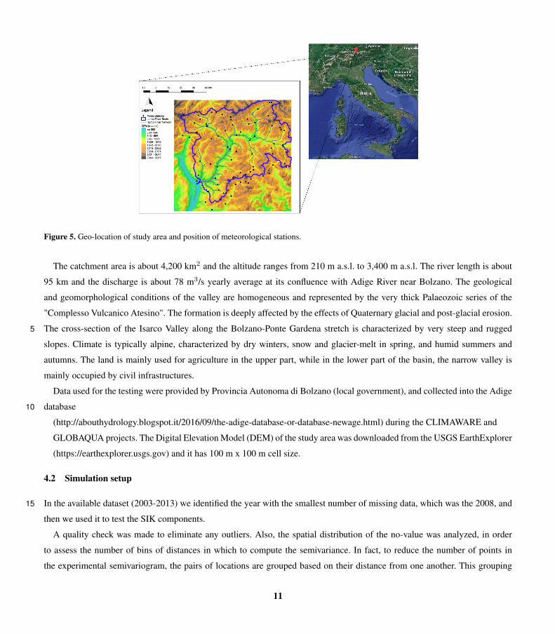
Figure 5. Geo-location of study area and position of meteorological stations.

The catchment area is about 4,200 km2 and the altitude ranges from 210 m a.s.l. to 3,400 m a.s.l. The river length is about

95 km and the discharge is about 78 m3/s yearly average at its confluence with Adige River near Bolzano. The geological

and geomorphological conditions of the valley are homogeneous and represented by the very thick Palaeozoic series of the

"Complesso Vulcanico Atesino". The formation is deeply affected by the effects of Quaternary glacial and post-glacial erosion.

The cross-section of the Isarco Valley along the Bolzano-Ponte Gardena stretch is characterized by very steep and rugged5

slopes. Climate is typically alpine, characterized by dry winters, snow and glacier-melt in spring, and humid summers and

autumns. The land is mainly used for agriculture in the upper part, while in the lower part of the basin, the narrow valley is

mainly occupied by civil infrastructures.

Data used for the testing were provided by Provincia Autonoma di Bolzano (local government), and collected into the Adige

database10

(http://abouthydrology.blogspot.it/2016/09/the-adige-database-or-database-newage.html) during the CLIMAWARE and

GLOBAQUA projects. The Digital Elevation Model (DEM) of the study area was downloaded from the USGS EarthExplorer

(https://earthexplorer.usgs.gov) and it has 100 m x 100 m cell size.

4.2 Simulation setup

In the available dataset (2003-2013) we identified the year with the smallest number of missing data, which was the 2008, and15

then we used it to test the SIK components.

A quality check was made to eliminate any outliers. Also, the spatial distribution of the no-value was analyzed, in order

to assess the number of bins of distances in which to compute the semivariance. In fact, to reduce the number of points in

the experimental semivariogram, the pairs of locations are grouped based on their distance from one another. This grouping

11

process is known as binning. For each time step, we found that about 10% of stations were not recording data. Therefore, since

the mean number of active stations for each time step was 70-80, we decided to use 8 bins. This choice was also supported by

a visual inspection of the shape of the experimental semivariance, which confirmed that by using 8 bins the number of stations

involved were neither too low nor too high.

In order to assess the goodness of SIK performances, two applications were performed:5

– an interpolation of one year of hourly temperature data;

– an interpolation of a rainfall event, also at hourly time steps.

Firstly, the analysis of the semivariance was performed and experimental semivariograms were fitted using all the 11 theo-

retical models. The model that gave the best fitting was then used for the interpolation of the temperature and rainfall variables

using the 4 types of Kriging. Kriging performances were assessed using the leave-one-out cross validation. The two local cases10

(LOK and LDK) were performed using a fixed number of closer stations. In particular, we decided to use 10 stations for the

temperature case, since it was a good compromise between the distance among the stations and the mean number of recording

stations for each time step. Regarding the local interpolation of precipitation, the number of closer stations was 5, given the

prevalently convective nature of summer precipitation and the lower number of active gauge stations for each time step. Finally,

results obtained from the interpolation of the temperature dataset were compared to the results obtained with R gstat, in order15

to assess the differences between the two packages, their easiness of use and their performances.

5 Simulations results

5.1 Application of SIK to a temperature dataset

The first application of SIK components was done using the temperature dataset. The hourly experimental semivariograms

were computed and then fitted using the 11 available theoretical models.20

Figure 6 shows the results of the fitting of the experimental semivariogram for a single time step on 15 June 2008. The black

dots represent the experimental semivariance, while each colored curve represents a different optimized theoretical model. The

Y and X axis show the values of the semivariance γ [h] and the distances in meters respectively.

12

Figure 6. Fitting of the experimental semivariogram using PSO for 15 June 2008 12:00 CET.

Table 1 reports the main indexes of goodness of fit (GOFs), namely NSE, RMSE, R2 and PBIAS, computed between the

experimental semivariogram and the 11 theoretical semivariogram models. The aforementioned GOFs are defined in Appendix

C and were obtained using the R package hydroGOF (https://cran.r-project.org/web/packages/hydroGOF/hydroGOF.pdf),

which computes the GOFs between measured and simulated values (in this case experimental semivariance and theoretical

semivariance). All the semivariogram models gave satisfactory results, with large values of NSE (0.72 : 0.92) and R2 (0.735

: 0.92), low values of RMSE (2.14 oC : 3.99 oC) and PBIAS (-3.80% : -7.90%), confirming the accuracy of the calibration

procedure.

Semivariogram NSE RMSE R2 PBIAS

Bessel 0.92 2.14 0.92 -0.20

Circular 0.88 2.59 0.88 0.0

Exponential 0.92 2.10 0.92 -3.80

Gaussian 0.90 2.39 0.91 0.35

Hole 0.77 3.61 0.81 7.90

Linear 0.91 2.28 0.91 0.0

Logarithmic 0.92 2.17 0.92 0.0

Pentaspherical 0.91 2.29 0.91 0.0

Periodic 0.90 2.18 0.92 0.0

Power 0.72 3.99 0.73 -3.70

Spherical 0.91 2.28 0.91 0.0Table 1. Performance results of semivariogram models used.

13

In order to asses the goodness of the interpolation, we performed the leave-one-out cross validation using the optimized

hourly values of sill, nugget and range for the Bessel model, which is one of the best semivariograms according to the previous

results.

Figure 7 shows the results for the four types of Kriging in terms of NSE. Each point represents the averaged monthly NSE

over the 97 meteorological stations. The two local cases were performed using the ten closest stations to the interpolation point.5

For both the OK and LOK cases the performances were very poor (NSE < 0.5), indicating that mean temperature might have

been a better predictor than the interpolation.

A strong trend between temperature and elevation (R2 ∼ 0.9) was detected during the quality check phase (which was

expected). Therefore, interpolation results obtained using the DK and the LDK present optimal higher values of the goodness

of fit index (maximum NSE of 0.93) compared to the OK and LOK cases.10

-0.5

0.0

0.5

1.0

1 2 3 4 5 6 7 8 9 10 11 12Month

NSE

OK

LOK

DK

LDK

Hourly temperature

Figure 7. Monthly variation of the NSE index over the entire hourly temperature dataset using the Bessel semivariogram model.

The spatialization of temperature was done for each pixel of the DEM, applying the LDK and the Bessel semivariogram

model. Figure 8 shows the maps obtained for two different dates in the 2008, one in winter (15 February 2008 12:00) and

one in summer (15 June 2008 12:00). The bubble plots of the RMSE obtained between the measured and the interpolated

values have been overlapped onto the maps. The size of a bubble represents the magnitude of the error: the largest error for the

interpolation of February 2008 (RMSE = 4.1 oC) corresponds to Station ID 90534 (Z=1385 m a.s.l.), while the largest error15

for June 2008 interpolation (RMSE = 3.2 oC) corresponds to Station ID 90266 (Z=490 m a.s.l.).

14

-12 10 0 10 19

Figure 8. Maps of spatialized temperature for 15 February 2008 and 15 June 2008. Two bubble plots are overlapped, which represent the

RMSE between the measured and interpolated values.

5.2 Application of SIK to a rainfall dataset

The application to a rainfall dataset was made at event scale; specifically, a rainfall event of 11 h between the 29 and 30 June

2008. The event was chosen because it was the longest and most intense recorded by the highest number of stations for 2008.

Figure 9 shows the boxplots of the 11 hourly semivariograms with 8 bins of lag distance, while the red line represents the

best theoretical semivariogram, which in this case was obtained using the Bessel model. The Y and X axis show the values of5

the semivariance γ [h] and the distances in [m], respectively.

15

.1 .2 .3 .4 .5 .6 .7

05

1015

20

Rain event: 30 h

Distance [m]

γ[h]

Rainevent:11h

Figure 9. Boxplots of the semivariograms of the precipitation event of 29th and 30th June 2008.

The optimized values of range, nugget and sill were then used for the 4 types of Kriging interpolations. Figure 10 compares

the results obtained for two stations (ID 1152 and ID 1270) chosen at different elevations (943 m a.s.l. and 2100 m a.s.l.,

respectively). All the interpolators were able to capture the rainfall peak at midnight for both stations. Comparing the volumes

of cumulative rainfall, shown in Table 2, all the interpolators gave good results for the station ID 1152, while there is an

overestimation in the case of station ID 1270; this is due to peaks detected but not recorded between the 21:00 and the 00:00.5

16

Figure 10. Comparison between the four types of Kriging and the measured rainfall.

Table 2 also shows the indexes of goodness of fit between the measured and the interpolated rainfall for the 4 types of

Kriging and the two stations. The performances are overall good in the case of station ID 1152 and the best interpolator is the

LDK computed using the 5 closest stations. Results for station ID 1270 are generally worse, with the highest NSE of 0.62 for

the LOK case. This could be due to the higher elevation of the station, which led to a series of interpolated peaks that were not

recorded.5

ID 1152 ID 1270

Kriging NSE RMSE R2 Cum (mm) NSE RMSE R2 Cum (mm)

OK 0.77 1.42 0.94 20 0.31 1.88 0.45 24

LOK 0.86 1.09 0.94 22 0.62 1.39 0.65 22

DK 0.80 1.33 0.83 22 0.46 1.66 0.54 20

LDK 0.91 0.92 0.92 25 0.35 1.82 0.37 13

Measured - - - 25 - - - 16Table 2. Results in terms of goodness of fit indexes between the measured and interpolated rainfall values for two stations.

The spatial interpolation of the precipitation was also done for each pixel of the DEM, applying the LOK and the Bessel

semivariogram model. Figure 11 shows the results of the interpolation for 30 June 2008 at 00:00. As it appears from the map,

the rainfall intensities are higher in the river valley, with a value of 9.8 mm/h measured at station ID 1152. The bubble plots

17

of the RMSE obtained between the measured and the interpolated values are overlapped. The size of a bubble represents the

magnitude of the error: the largest error is obtained for station ID 90133 (Z=1246 m a.s.l.).

Precipitation(mm/h)

Figure 11. Spatial interpolation of the precipitation applying LOK and the Bessel semivariogram model. The bubble plot of the RMSE is

overlapped.

6 A qualitative comparison with the R package gstat

“A comparison between SIK and the R package gstat was made in order to highlight their differences and similarities, and to

justify the deployment of an alternative software. We performed a qualitative comparison between the two softwares accounting5

for design, the implemented features, and the accuracy of the results. Benchmarks or quantitative performance comparisons

18

would not have been useful or completely truthful since the "velocity" of computation (a classic quantitative comparison)

depends on too many factors, some of which are described below. Moreover, in our opinion, the two tools that we analyzed

have different purposes. This can be seen just by looking at the features of the relative programming languages. The gstat

software is developed in C with a part of the code in R language. It must be executed using the various R environments. SIK

is developed in Java (7) as a group of OMS components and it can be executed within the OMS console, as a stand-alone Java5

programs, or embedded in other codes in languages that support Java bindings. Java is slower than 3rd generation languages

such as C. However, in the course of Java development several optimizations, such as “just-in-time compilation” and “adaptive

optimization”, have been introduced to improve the performance of its Java Virtual Machine (JVM). These techniques identify

recurrently executed algorithms, so called “hot spots”, and dynamically recompile them at run-time. Eventually, the hot spots

gain valuable computational speed. C is one of the fastest compiled languages. But only the computational core of gstat is10

coded in C; the management of temporal steps, such as “for-loops”, and data structures must be scripted in R. Undoubtedly,

R is a very powerful programming language, mainly because of its flat learning curve, and easy syntax and semantics, but it

is fully interpreted, which makes it very slow. As a result, the comparison of the speed of computation for a single temporal

Kriging interpolation is unfair against Java, since the JVM cannot exploit its optimization tools for a single computation. On

the other hand, the comparison of the speed of computation for a year of hourly Kringing interpolations is biased against R,15

because temporal steps affect most of the computational time. In terms of functionality, gstat computes both omnidirectional

and directional semivariongrams, while SIK does not implement directional semivariograms yet (although we have included

this feature on the software wish list). Furthermore, gstat provides four more theoretical semivariogram models with respect to

SIK: Matern, Matern with Stein’s parameterizations, Wave, and Legendre. Adding the desired theoretical model to any SIK-TV

component would be easy and straightforward, thanks to the DP implemented, as shown in Figure 2, but they are not available20

yet. Regarding the estimates that the two packages offer, these are usually different. Comparisons were made with both the

temperature and rainfall datasets used in section 4. Semivariograms were computed using the same number of bins and cutoff

distance.

Figure 12 shows the results of the temperature interpolations done with SIK and gstat, in terms of NSE, RMSE, PBIAS

and R2: the overall performances of both tools are very good. The NSE values are always above the 0.65, while the RMSE are25

always lower then 2 oC.

19

Figure 12. Comparison between the performances of gstat and SIK packages in the interpolation of the temperature dataset.

Figure 13 shows the results of the precipitation interpolation done with SIK and gstat, in terms of NSE, RMSE, PBIAS, R2

and cumulative volumes. Also in this case, both softwares are able to reproduce the rainfall event well, simulating the peaks.

The results obtained for station ID 1152 are very good for both softwares, with a NSE >0.9. Both softwares show slightly

worse results for station ID 2170, with lower values of NSE and R2, higher RMSE, and an overestimation of the total rainfall

(19 mm with gstat and 20 mm with SIK, compared to the 16 mm recorded by the gauges).5

In conclusion, gstat is a powerful, flexible tool to get fast results with fast scripting in answer to single, specific questions

(with some implementation efforts user-side); SIK is a tool that is ready to be integrated into broader MS, specifically because

of its OMS-compliant design. The interpolations of both temperature and rainfall confirm the quality and accuracy of the

predictions obtained using the SIK package, demonstrating that it is a good competitor of R gstat.

20

gstat SIKRMSE 0.88 1.39NSE 0.85 0.62R2 0.86 0.65

Cum (mm) 19 20

  gstat SIKRMSE 0.65 0.92NSE 0.95 0.91R2 0.96 0.92

Cum (mm) 22 25

Figure 13. Comparison between the performances of gstat and SIK packages in the interpolation of the rainfall dataset.

7 Conclusions

This paper presents a new modelling package for the spatial interpolation of environmental variables. It includes 11 theoretical

semivariogram models and 4 types of Kriging interpolations. To test the performance of the SIK package, two applications

were performed: the interpolation of one year of temperatures and the interpolation of a rainfall event. Data were retrieved

from a dataset of 97 stations located in the Isarco Valley in Italy and the resolution of the interpolation grid data was 100 m.5

Several characteristics make the SIK package a good competitor tool among those available in the literature. From the user

perspective:

– it can be used as a stand-alone;

– it can plugged-in to the hydrological modeling system GEOframe-NewAGE;

– it can be used with all OMS compliant components, such as calibration tools for the optimization of the parameters;10

– it includes a tool for the automatic estimation of errors;

– its results are presented in data formats that can be visualized directly by GIS;

– a variety of MS can be obtained, according to user needs;

– it is faster than gstat in every-day use routine, under certain conditions.

From the programmer perspective, the implementation of DP makes the package easy to maintain and suitable for future15

improvements. All the elements are close to modification and open to extension. Further developments of the package are easy

21

and straightforward. Examples of such developments might include: integrating new types of Kriging, implementing a different

selection method of the gauge stations, and the addition of non-linear relationships between the interpolated variable and an

auxiliary variable.

The interpolations of both the temperature and the rainfall gave very good results, with a high agreement between the

measured and the interpolated variables. The tests also show how it is possible to choose between 11 variograms and four5

Kriging alternatives and to compare the outcomes easily. On the other hand, the single rainfall event did not show trend with

elevation.

In comparison with gstat, the SIK package proved to be a good alternative, regarding both the easiness of use and the

accuracy of the interpolation.

Computer Code Availability10

An OSF project with all the components needed to reproduce the results shown in this paper has been created and is available

at the following link: https://osf.io/24rgv. The interested researcher can find the entire OMS project, containing input data,

output, sim files, jar files and R script used for the plots. Moreover, the links to the source codes and to the documentation of

the SIK components are also available in the OSF project. In particular, for the present work, version 0.9.8 is the version of the

codes of the GEOframe-SIK package that we used, available at the following link: https://github.com/geoframecomponents/15

Krigings/tree/v0.9.8.

Author contribution

Marialaura Bancheri, Giuseppe Formetta and Francesco Serafin developed the model code integrated in the GEOframe-SIK

package. Marialaura Bancheri, Francesco Serafin, Michele Bottazzi and Wuletawu Abera designed the experiments and per-

formed the simulations. Riccardo Rigon planned the research, coordinated and supervised all its phases, and provided the20

financial support with his funding. Marialaura Bancheri prepared the manuscript with contributions from all co-authors. Lastly,

the authors declare that they have no conflict of interest.

Acknowledgments

The authors acknowledge Trento University project CLIMAWARE

(http://abouthydrology.blogspot.it/search/ label/CLIMAWARE) and European Union FP7 Collaborative Project GLOBAQUA25

(Managing the effects of multiple stressors on aquatic ecosystems under water scarcity, grant no. 603629-ENV- 2013.6.2.1)

that partially financed this research.

22

Appendix A: Kriging theory

Kriging is a group of geostatistical techniques used to interpolate the value of random fields based on spatial autocorrelation

of measured data, (Isaaks and Srivastava, 1989; Goovaerts, 1997; Kitanidis, 1997). The measurements value z(xα) and the

unknown value z(x), where x is the location given according to a certain cartographic projection, are considered as particular

realizations of the random variables Z(xα) and Z(x) (Isaaks and Srivastava, 1989; Goovaerts, 1997). Let the estimation of5

the (true) random variable Z(x) be Zλ(x). It is obtained as a linear combination of the N random variables at surrounding

points, denoted as xα with α= {1,N}, as in Goovaerts (1999):

Zλ(x)−m(x) =N∑α=1

λα(xα)[Z(xα)−m(xα)] (A1)

where m(x) and m(xα) are the expected values of the random variables Z(x) and Z(xα); λ(xα) at varying α is the N-uple

of weights assigned to the random variable Z(xα) at measured sites. The superscript λ in Zλ(x) denotes that this new random10

variable is parameterized by the weights. These are chosen to satisfy the condition of minimizing the error of variance of the

estimator σ2λ, that is:

argminλ

σ2λ ≡ argmin

λV ar[Zλ(x)−Z(x)] (A2)

under the constraint that the estimate is unbiased, i.e.,

E[Zλ(x)−Z(x)] = 0 (A3)15

The latter condition, implies that:

N∑α=1

λα(xα) = 1 (A4)

As shown in various textbooks, e.g., Kitanidis (1997), the above conditions bring to a linear system with the unknown being

the N-uple of weights, and the system matrix dependent on the semivariograms (defined below in a simplified case).In synthetic

notation, the linear system can be written as:20

ΓΛ =B (A5)

where Γ is the matrix of two point variograms (defined below), Λ is the N-uple of unknown weights and B (the so called

known term) is an N-uple containing the variograms between the ungauged site and the measured sites. Further information is

required for (A5) to be a solvable linear system. In fact, B is still unknown at this stage.

If isotropy of the spatial statistics of the quantity analyzed is assumed, then the semivariogram is given by, (e.g., Cressie25

and Cassie (1993)):

γ(h) =1

2Nh

Nh∑i=1

[Z(x)−Z(xi)]2 (A6)

23

where Nh denotes the number of observation points at location xi at distance h from x for any h. When random variables are

substituted by their available realizations (i.e. z(xi), indicated with normal letters) an empirical semivariogram is obtained. In

order to be extended to any distance, γ [h] needs to be fitted to a theoretical semivariogram model, i.e. an assumed function

form, as those detailed in Appendix D. The fitting to the theoretical semivariogram model is also necessary to get B. In

fact, when a theoretical semivariogram is selected, only position information for the ungauged location is required to get its5

semivariogram with respect to any of the measured locations.

Once B has been determined, the system (A5) can be solved. This procedure is clearly delineated in literature and explained

for instance in Kitanidis (1997). Optimized semivariogram models are used to estimate the weighted parameters of kriging

algorithm.

Appendix B: List of acronyms10

Acronyms Meaning

m a.s.l. meter above sea level

CET central European time

DEM digital elevation model

DK detrended kriging

DOI digital object identifier

DP design patterns

GIS geographical information systems

LDK local detrended kriging

LOK local ordinary kriging

LOO leave-one-out

MS modeling solutions

NSE Nash-Sutcliffe efficiency

OMS3 object modeling system v.3

OK ordinary kriging

PBIAS percent bias

PSO particle swarm optimization

R2 coefficient of determination

RMSE root mean square error

SIK spatial interpolation kriging

24

Appendix C: Goodness of fit indices

– Coefficient of determination

The coefficient of determination, R2, is the proportion of variance in the dependent variable that is predictable from the

independent variable(s):

R2 = 1−∑ni=1(Mi−Si)2∑ni=1(Mi−Mi)2

(C1)5

where Mi is the true value, Mi is the mean of Mi and Si is the predicted value. It varies between 0 to 1, where 1

corresponds to the maximum agreement between predicted and true values.

– Nash - Sutcliffe efficiency

The Nash-Sutcliffe Efficiency (NSE) is a normalized model efficiency coefficient. It determines the relative magnitude

of the residual variance compared to the measured data variance (Nash and Sutcliffe, 1970)10

NSE = 1−∑ni=1(Si−Mi)

2∑ni=1(Mi−Mi)2

(C2)

where Si is the predicted value and Mi is the observed value at a given time step. It varies from −∞ to 1, where 1

corresponds to the maximum agreement between predicted and observed values.

– Percentage bias

Percent bias (PBIAS) measures the average tendency of the simulated values to be larger or smaller than the correspond-15

ing measured ones. The optimal value of PBIAS is 0, with small values indicating accurate model simulation. Positive

values indicate overestimation bias, while negative values indicate model underestimation bias.

PBIAS = 100 ·

N∑i=1

(Si−Mi)

N∑i=1

Mi

(C3)

where Si is the predicted value and Mi is the observed value.

– Root mean square error20

The Root Mean Square Error (RMSE) is given by:

RMSE =

√√√√ 1

N

N∑i=1

(Mi−Si)2 (C4)

25

where M and S represent the measured and simulated time-series respectively and N is the number of components in the

series.

Appendix D: List of semivariogram models implemented in SIK

Using n to represent nugget, h to represent lag distance, r to represent range, and s to represent sill, the 11 theoretical semi-

variogram models most frequently used in literature are:5

– Bessel semivariogram

γ(h) = s

(1− h

rk1

(h

r

))(D1)

– Circular semivariogramγ(h) = n+ s

{2π

[hr

√1−

(hr

)2]+ arcsin

(hr

)}h < r

γ(h) = n+ s h≥ r(D2)

– Exponential semivariogram10

γ(h) = n+ s(1− e−hr ) (D3)

– Gaussian semivariogram

γ(h) = n+ s[1− e−(hr )

2

] (D4)

– Hole semivariogram

γ(h) = n+ s

[1−

sin(hr )hr

](D5)15

– Linear semivariogramγ(h) = n+ shr h < r

γ(h) = n+ s h≥ r(D6)

– Logarithmic semivariogram

γ(h) = n+ s log

(h

r

)(D7)

26

– Pentaspherical semivariogramγ(h) = n+ s

{158hr +

(hr

)3[− 5

4 + 38

(hr

)5]}h < r

γ(h) = n+ s h≥ r(D8)

– Periodic semivariogram

γ(h) = n+ s

[1− cos

(2πh

r

)](D9)

– Power semivariogram5

γ(h) = n+ shr (D10)

– Spherical semivariogramγ(h) = n+ s

[1.5hr − 0.5

(hr

)3]h < r

γ(h) = n+ s h≥ r(D11)

27

References

Abera, W., Formetta, G., Borga, M., and Rigon, R.: Estimating the water budget components and their variability in a pre-alpine basin with

JGrass-NewAGE, Advances in Water Resources, 104, 37–54, 2017.

Adams, B. M., Bohnhoff, W., Dalbey, K., Eddy, J., Eldred, M., Gay, D., Haskell, K., Hough, P. D., and Swiler, L. P.: Dakota, a multilevel

parallel object-oriented framework for design optimization, parameter estimation, uncertainty quantification, and sensitivity analysis:5

Version 5.0 user’s manual, Sandia National Laboratories, Tech. Rep. SAND2010-2183, 2009.

Adhikary, S. K., Muttil, N., and Yilmaz, A. G.: Genetic programming-based ordinary kriging for spatial interpolation of rainfall, Journal of

Hydrologic Engineering, 21, 04015 062, 2015.

Aidoo, E. N., Mueller, U., Goovaerts, P., and Hyndes, G. A.: Evaluation of geostatistical estimators and their applicability to characterise the

spatial patterns of recreational fishing catch rates, Fisheries Research, 168, 20–32, 2015.10

Argent, R. M.: An overview of model integration for environmental applications—components, frameworks and semantics, Environmental

Modelling & Software, 19, 219–234, 2004.

Attorre, F., Alfo, M., De Sanctis, M., Francesconi, F., and Bruno, F.: Comparison of interpolation methods for mapping climatic and biocli-

matic variables at regional scale, International Journal of Climatology, 27, 1825–1843, 2007.

Balme, M., Vischel, T., Lebel, T., Peugeot, C., and Galle, S.: Assessing the water balance in the Sahel: Impact of small scale rainfall variability15

on runoff: Part 1: Rainfall variability analysis, Journal of Hydrology, 331, 336–348, 2006.

Bancheri, M.: A flexible approach to the estimation of water budgets and its connection to the travel time theory, Ph.D. thesis, University of

Trento, 2017.

Basistha, A., Arya, D., and Goel, N.: Spatial distribution of rainfall in Indian himalayas–a case study of Uttarakhand region, Water Resources

Management, 22, 1325–1346, 2008.20

Beck, K.: Test-driven development: by example, Addison-Wesley Professional, 2003.

Boer, E. P., de Beurs, K. M., and Hartkamp, A. D.: Kriging and thin plate splines for mapping climate variables, International Journal of

Applied Earth Observation and Geoinformation, 3, 146–154, 2001.

Buytaert, W., Celleri, R., Willems, P., Bièvre, B. D., and Wyseure, G.: Spatial and temporal rainfall variability in mountainous areas: A case

study from the south Ecuadorian Andes, Journal of Hydrology, 329, 413–421, 2006.25

Carrera-Hernández, J. and Gaskin, S.: Spatio temporal analysis of daily precipitation and temperature in the Basin of Mexico, Journal of

Hydrology, 336, 231–249, 2007.

Cressie, N. A. and Cassie, N. A.: Statistics for spatial data, vol. 900, Wiley New York, 1993.

Creutin, J. and Obled, C.: Objective analyses and mapping techniques for rainfall fields: an objective comparison, Water Resources Research,

18, 413–431, 1982.30

David, O., Ascough Ii, J., Lloyd, W., Green, T., Rojas, K., Leavesley, G., and Ahuja, L.: A software engineering perspective on environmental

modeling framework design: The Object Modeling System, Environmental Modelling & Software, 39, 201–213, 2013.

Deutsch, C. V. and Journel, A. G.: Geostatistical software library and user&s guide, vol. 1996, Oxford university press New York, 1992.

Di Piazza, A., Conti, F. L., Noto, L., Viola, F., and La Loggia, G.: Comparative analysis of different techniques for spatial interpolation

of rainfall data to create a serially complete monthly time series of precipitation for Sicily, Italy, International Journal of Applied Earth35

Observation and Geoinformation, 13, 396–408, 2011.

28

Donatelli, M. and Rizzoli, A.-E.: A design for framework-independent model components of biophysical systems, in: Proceedings of the

iEMSs Fourth Biennial Meeting, Barcelona, Catalonia. International Congress on Environmental Modelling and Software iEMSs 2008.,

pp. 727–734, 2008.

Eberhart, R. and Kennedy, J.: A new optimizer using particle swarm theory, in: Micro Machine and Human Science, 1995. MHS’95.,

Proceedings of the Sixth International Symposium on, pp. 39–43, IEEE, 1995.5

Eckel, B.: Thinking in JAVA, Prentice Hall Professional, 2003.

Efron, B.: The jackknife, the bootstrap and other resampling plans, vol. 38, SIAM, 1982.

Eischeid, J. K., Pasteris, P. A., Diaz, H. F., Plantico, M. S., and Lott, N. J.: Creating a serially complete, national daily time series of

temperature and precipitation for the western United States, Journal of Applied Meteorology, 39, 1580–1591, 2000.

Ellis, B., Stylos, J., and Myers, B.: The factory pattern in API design: A usability evaluation, in: Proceedings of the 29th international10

conference on Software Engineering, pp. 302–312, IEEE Computer Society, 2007.

Formetta, G., Rigon, R., Chávez, J., and David, O.: Modeling shortwave solar radiation using the JGrass-NewAge system, Geoscientific

Model Development, 6, 915–928, 2013.

Formetta, G., Antonello, A., Franceschi, S., David, O., and Rigon, R.: Hydrological modelling with components: A GIS-based open-source

framework, Environmental Modelling & Software, 55, 190–200, 2014.15

Formetta, G., Bancheri, M., David, O., and Rigon, R.: Site specific parameterizations of longwave radiation, 2016.

Freeman, E., Robson, E., Bates, B., and Sierra, K.: Head First Design Patterns: A Brain-Friendly Guide, " O’Reilly Media, Inc.", 2004.

Gamma, E.: Design patterns: elements of reusable object-oriented software, Pearson Education India, 1994.

Gardner, H. and Manduchi, G.: Design Patterns for e-Science, 2002.

Goovaerts, P.: Geostatistics for natural resources evaluation, Oxford university press, 1997.20

Goovaerts, P.: Geostatistics in soil science: state-of-the-art and perspectives, Geoderma, 89, 1–45, 1999.

Goovaerts, P.: Geostatistical approaches for incorporating elevation into the spatial interpolation of rainfall, Journal of Hydrology, 228,

113–129, 2000.

Gräler, B., Pebesma, E., and Heuvelink, G.: Spatio-Temporal Interpolation using gstat, The R Journal, 8, 204–218, https://journal.r-project.

org/archive/2016-1/na-pebesma-heuvelink.pdf, 2016.25

Haberlandt, U.: Geostatistical interpolation of hourly precipitation from rain gauges and radar for a large-scale extreme rainfall event, Journal

of Hydrology, 332, 144–157, 2007.

Hall, D. K., Riggs, G. A., and Salomonson, V. V.: MODIS snow and sea ice products, in: Earth science satellite remote sensing, pp. 154–181,

Springer, 2006.

Hevesi, J. A., Istok, J. D., and Flint, A. L.: Precipitation estimation in mountainous terrain using multivariate geostatistics. Part I: structural30

analysis, Journal of Applied Meteorology, 31, 661–676, 1992.

Hutchinson, M.: Interpolating mean rainfall using thin plate smoothing splines, International Journal of Geographical Information Systems,

9, 385–403, 1995.

Isaaks, E. H. and Srivastava, R. M.: An introduction to applied geostatistics, vol. 561, Oxford University Press New York, 1989.

Jarvis, C. H. and Stuart, N.: A comparison among strategies for interpolating maximum and minimum daily air temperatures. Part I: The35

selection of “guiding” topographic and land cover variables, Journal of Applied Meteorology, 40, 1060–1074, 2001.

Kitanidis, P. K.: Introduction to geostatistics: applications in hydrogeology, Cambridge University Press, 1997.

29

Krige, D. G.: A statistical approach to some basic mine valuation problems on the Witwatersrand, Journal of the Southern African Institute

of Mining and Metallurgy, 52, 119–139, 1951.

Li, J. and Heap, A. D.: A review of comparative studies of spatial interpolation methods in environmental sciences: performance and impact

factors, Ecological Informatics, 6, 228–241, 2011.

Lloyd, C.: Assessing the effect of integrating elevation data into the estimation of monthly precipitation in Great Britain, Journal of Hydrol-5

ogy, 308, 128–150, 2005.

Ly, S., Charles, C., and Degre, A.: Geostatistical interpolation of daily rainfall at catchment scale: the use of several variogram models in the

Ourthe and Ambleve catchments, Belgium, Hydrology & Earth System Sciences, 15, 2011.

Ly, S., Charles, C., and Degré, A.: Different methods for spatial interpolation of rainfall data for operational hydrology and hydrological

modeling at watershed scale. A review, 2013.10

Martin, J. D. and Simpson, T. W.: A study on the use of kriging models to approximate deterministic computer models, in: Proceedings of

DETC, vol. 3, pp. 2–6, 2003.

Martin, R. C.: Agile software development: principles, patterns, and practices, Prentice Hall, 2002.

Matheron, G.: Splines and kriging: their formal equivalence, Down-to-earth statistics: solutions looking for geological problems, 8, 77–95,

1981.15

Meyer, M.: Continuous integration and its tools, IEEE software, 31, 14–16, 2014.

Mitášová, H. and Mitáš, L.: Interpolation by regularized spline with tension: I. Theory and implementation, Mathematical Geology, 25,

641–655, 1993.

Murphy, B.: PyKrige: development of a kriging toolkit for Python, in: AGU fall meeting abstracts, 2014.

Nash, J. and Sutcliffe, J.: River flow forecasting through conceptual models part I — A discussion of principles, Journal of Hydrol-20

ogy, 10, 282 – 290, https://doi.org/http://dx.doi.org/10.1016/0022-1694(70)90255-6, http://www.sciencedirect.com/science/article/pii/

0022169470902556, 1970.

Pebesma, E. J.: Multivariable geostatistics in S: the gstat package, Computers & Geosciences, 30, 683–691, 2004.

Phillips, D. L., Dolph, J., and Marks, D.: A comparison of geostatistical procedures for spatial analysis of precipitation in mountainous

terrain, Agricultural and Forest Meteorology, 58, 119–141, 1992.25

Robeson, S. M.: Spatial interpolation, network bias, and terrestrial air temperature variability, 1992.

Rouson, D., Xia, J., and Xu, X.: Scientific software design: the object-oriented way, Cambridge University Press, 2011.

Saghafian, B. and Bondarabadi, S. R.: Validity of regional rainfall spatial distribution methods in mountainous areas, Journal of Hydrologic

Engineering, 13, 531–540, 2008.

Schymanski, S. J. and Or, D.: Leaf-scale experiments reveal an important omission in the Penman-Monteith equation, Hydrology and Earth30

System Sciences, 21, 685, 2017.

Stahl, K., Moore, R., Floyer, J., Asplin, M., and McKendry, I.: Comparison of approaches for spatial interpolation of daily air temperature in

a large region with complex topography and highly variable station density, Agricultural and Forest Meteorology, 139, 224–236, 2006.

Stooksbury, D. E., Idso, C. D., and Hubbard, K. G.: The effects of data gaps on the calculated monthly mean maximum and minimum

temperatures in the continental United States: A spatial and temporal study, Journal of Climate, 12, 1524–1533, 1999.35

Tabios, G. Q. and Salas, J. D.: A comparative analysis of techniques for spatial interpolation of precipitation1, 1985.

Thiessen, A. H.: Precipitation averages for large areas, Monthly weather review, 39, 1082–1089, 1911.

30

Todini, E.: Influence of parameter estimation uncertainty in Kriging: Part 1-Theoretical Development, Hydrology and Earth System Sciences

Discussions, 5, 215–223, 2001.

Turk, F. J. and Miller, S. D.: Toward improved characterization of remotely sensed precipitation regimes with MODIS/AMSR-E blended

data techniques, IEEE Transactions on Geoscience and Remote Sensing, 43, 1059–1069, 2005.

Van Ittersum, M. K., Ewert, F., Heckelei, T., Wery, J., Olsson, J. A., Andersen, E., Bezlepkina, I., Brouwer, F., Donatelli, M., Flichman, G.,5

et al.: Integrated assessment of agricultural systems–A component-based framework for the European Union (SEAMLESS), Agricultural

systems, 96, 150–165, 2008.

Verfaillie, E., Van Lancker, V., and Van Meirvenne, M.: Multivariate geostatistics for the predictive modelling of the surficial sand distribution

in shelf seas, Continental Shelf Research, 26, 2454–2468, 2006.

WMO: WMO. 1994: Guide to hydrological practices: Data acquisition and processing, analysis, forecasting and other applications. WMO10

Publication No. 168., 1994.

Xu, C.-Y. and Singh, V. P.: A review on monthly water balance models for water resources investigations, Water Resources Management, 12,

20–50, 1998.

31