Embed Size (px)
Citation preview

3The population of the United States has been increasing
since 1790, when the first census was taken. Over the past
few decades, the population has not only been increasing,
but the level of diversity has also been increasing. This fact
is important to school districts, businesses, and government
officials. Using examples in the third section of this chapter,
we explore two rates of change related to the increase in
minority population. In the first example, we calculate an
average rate of change; in the second, we calculate the rate
of change at a particular time. This latter rate is an example
of a derivative, the subject of this chapter.
3.1 Limits
3.2 Continuity
3.3 Rates of Change
3.4 Definition of the Derivative
3.5 Graphical Differentiation
Chapter 3 Review
Extended Application: A Model for Drugs Administered Intravenously
The Derivative
133
M03_LIAL8774_11_AIE_C03_133-208.indd 133 23/06/15 11:30 AM
Not for Sale
Copyright Pearson. All rights reserved.
ChAptER 3 the Derivative 134
the algebraic problems considered in earlier chapters dealt with static situations:
■ What is the revenue when 100 items are sold?■ how much interest is earned in three years?■ What is the equilibrium price?
Calculus, on the other hand, deals with dynamic situations:
■ At what rate is the demand for a product changing?■ how fast is a car moving after 2 hours?■ When does the growth of a population begin to slow down?
the techniques of calculus allow us to answer these questions, which deal with rates of change.
the key idea underlying calculus is the concept of limit, so we will begin by studying limits.
LimitsWhat happens to the demand of an essential commodity as its price continues to increase?
APPLY IT
3.1
We will find an answer to this question in Exercise 84 using the concept of limit.
The limit is one of the tools that we use to describe the behavior of a function as the values of x approach, or become closer and closer to, some particular number.
Finding a Limit
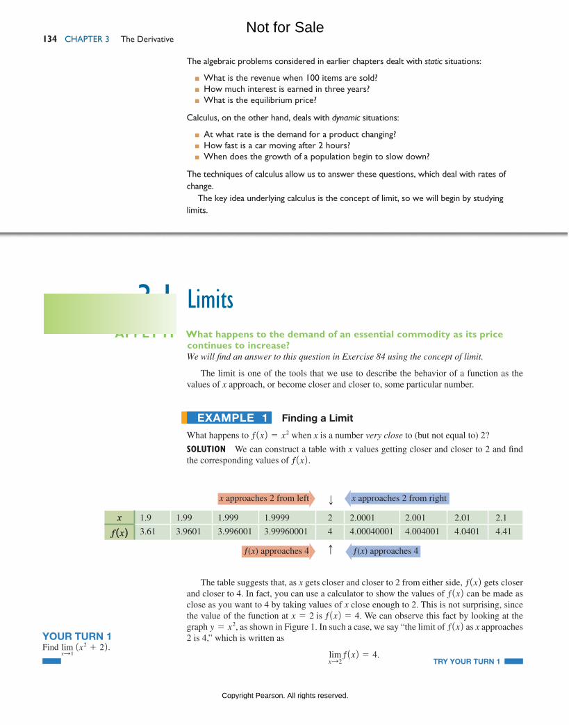
What happens to ƒ1x2 = x2 when x is a number very close to (but not equal to) 2?
Solution We can construct a table with x values getting closer and closer to 2 and find the corresponding values of ƒ1x2.
ExampLE 1
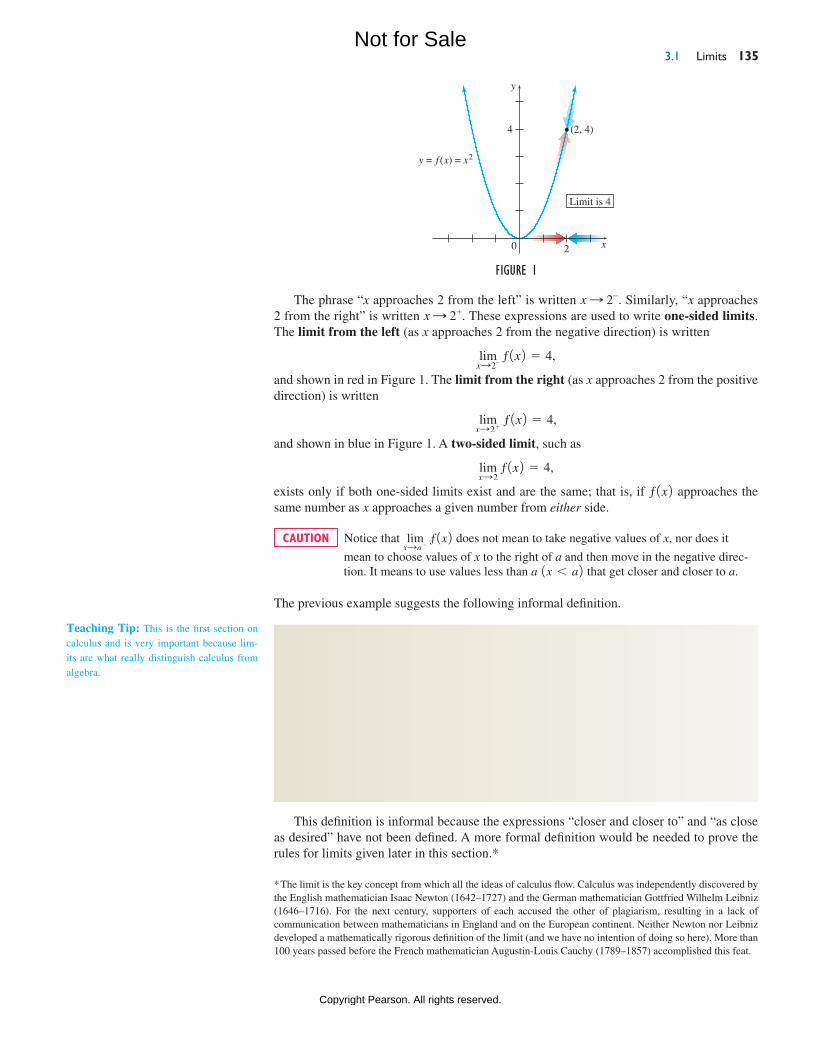
The table suggests that, as x gets closer and closer to 2 from either side, ƒ1x2 gets closer and closer to 4. In fact, you can use a calculator to show the values of ƒ1x2 can be made as close as you want to 4 by taking values of x close enough to 2. This is not surprising, since the value of the function at x = 2 is ƒ1x2 = 4. We can observe this fact by looking at the graph y = x2, as shown in Figure 1. In such a case, we say “the limit of ƒ1x2 as x approaches 2 is 4,” which is written as
limxS2
ƒ1x2 = 4. TRY YOUR TURN 1
YOUR TURN 1Find lim
xS1 1x2 + 22.
x 1.9 1.99 1.999 1.9999 2 2.0001 2.001 2.01 2.1
ƒ 1x 2 3.61 3.9601 3.996001 3.99960001 4 4.00040001 4.004001 4.0401 4.41
x approaches 2 from left x approaches 2 from right
ƒ(x) approaches 4 ƒ(x) approaches 4Sd
M03_LIAL8774_11_AIE_C03_133-208.indd 134 23/06/15 11:30 AM
Not for Sale
Copyright Pearson. All rights reserved.
3.1 Limits 135
The phrase “x approaches 2 from the left” is written x S 2-. Similarly, “x approaches 2 from the right” is written x S 2+. These expressions are used to write one-sided limits. The limit from the left (as x approaches 2 from the negative direction) is written
limxS2- ƒ1x2 = 4,
and shown in red in Figure 1. The limit from the right (as x approaches 2 from the positive direction) is written
limxS2 + ƒ1x2 = 4,
and shown in blue in Figure 1. A two-sided limit, such as
limxS2
ƒ1x2 = 4,
exists only if both one-sided limits exist and are the same; that is, if ƒ1x2 approaches the same number as x approaches a given number from either side.
Notice that limxSa - ƒ1x2 does not mean to take negative values of x, nor does it
mean to choose values of x to the right of a and then move in the negative direc-tion. It means to use values less than a 1x 6 a2 that get closer and closer to a.
The previous example suggests the following informal definition.
Limit of a FunctionLet ƒ be a function and let a and L be real numbers. If
1. as x takes values closer and closer (but not equal) to a on both sides of a, the corresponding values of ƒ1x2 get closer and closer (and perhaps equal) to L; and
2. the value of ƒ1x2 can be made as close to L as desired by taking values of x close enough to a;
then L is the limit of ƒ1x2 as x approaches a, written
limxSa
ƒ 1x 2 = L.
This definition is informal because the expressions “closer and closer to” and “as close as desired” have not been defined. A more formal definition would be needed to prove the rules for limits given later in this section.*
caution
Figure 1
y = f (x) = x2
20 x
4 (2, 4)
Limit is 4
y
Teaching Tip: This is the first section on calculus and is very important because lim-its are what really distinguish calculus from algebra.
* The limit is the key concept from which all the ideas of calculus flow. Calculus was independently discovered by the English mathematician Isaac Newton (1642–1727) and the German mathematician Gottfried Wilhelm Leibniz (1646–1716). For the next century, supporters of each accused the other of plagiarism, resulting in a lack of communication between mathematicians in England and on the European continent. Neither Newton nor Leibniz developed a mathematically rigorous definition of the limit (and we have no intention of doing so here). More than 100 years passed before the French mathematician Augustin-Louis Cauchy (1789–1857) accomplished this feat.
M03_LIAL8774_11_AIE_C03_133-208.indd 135 23/06/15 11:30 AM
Not for Sale
Copyright Pearson. All rights reserved.
ChAptER 3 the Derivative 136
The definition of a limit describes what happens to ƒ1x2 when x is near, but not equal to, the value a. It is not affected by how (or even whether) ƒ1a2 is defined. Also the definition implies that the function values cannot approach two different numbers, so that if a limit exists, it is unique. These ideas are illustrated in the following examples.
Note that the limit is a value of y, not x.
Finding a Limit
Find limxS2
g1x2, where g1x2 =x3 - 2x2
x - 2 .
Solution
The function g1x2 is undefined when x = 2, since the value x = 2 makes the denominator 0. However, in determining the limit as x approaches 2 we are concerned only with the values of g1x2 when x is close to but not equal to 2. To determine if the limit exists, consider the value of g at some numbers close to but not equal to 2, as shown in the following table.
caution
ExampLE 2
Method 1 using a table
Notice that this table is almost identical to the previous table, except that g is undefined at x = 2. This suggests that lim
xS2 g1x2 = 4, in spite of the fact that the function g does not exist
at x = 2.
A second approach to this limit is to analyze the function. By factoring the numerator,
x3 - 2x2 = x21x - 22,g1x2 simplifies to
g1x2 =x21x - 22
x - 2= x2, provided x Z 2.
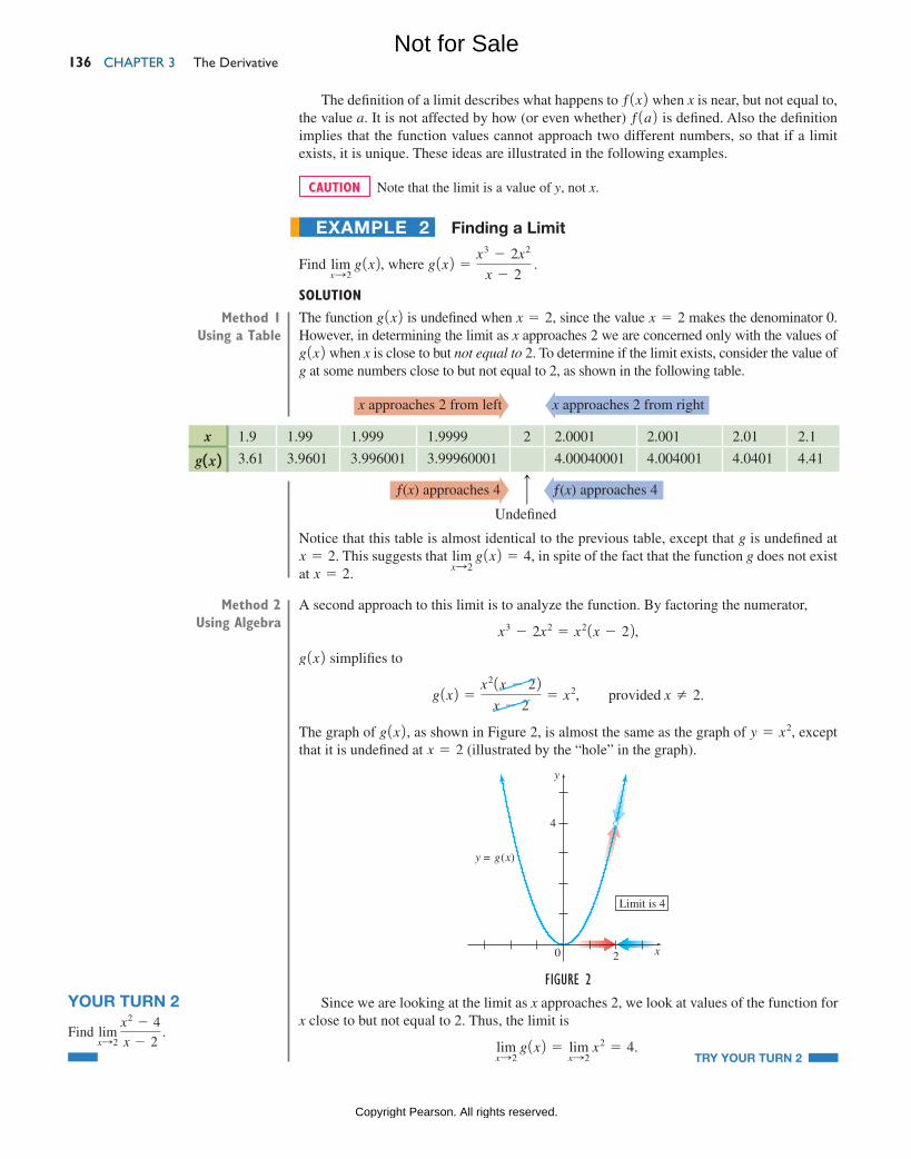
The graph of g1x2, as shown in Figure 2, is almost the same as the graph of y = x2, except that it is undefined at x = 2 (illustrated by the “hole” in the graph).
Method 2 using algebra
Figure 2
y = g(x)
20 x
4
Limit is 4
y
Since we are looking at the limit as x approaches 2, we look at values of the function for x close to but not equal to 2. Thus, the limit is
limxS2
g1x2 = limxS2
x2 = 4.
TRY YOUR TURN 2
YOUR TURN 2
Find limxS2
x2 - 4
x - 2 .
x 1.9 1.99 1.999 1.9999 2 2.0001 2.001 2.01 2.1
g 1x 2 3.61 3.9601 3.996001 3.99960001 4.00040001 4.004001 4.0401 4.41
x approaches 2 from left x approaches 2 from right
ƒ(x) approaches 4 ƒ(x) approaches 4
Undefined¡
M03_LIAL8774_11_AIE_C03_133-208.indd 136 23/06/15 11:30 AM
Not for Sale
Copyright Pearson. All rights reserved.
3.1 Limits 137
Note that a limit can be found in three ways:
1. algebraically;
2. using a graph (either drawn by hand or with a graphing calculator); and
3. using a table (either written out by hand or with a graphing calculator).
Which method you choose depends on the complexity of the function and the accuracy required by the application. Algebraic simplification gives the exact answer, but it can be difficult or even impossible to use in some situations. Calculating a table of numbers or trac-ing the graph may be easier when the function is complicated, but be careful, because the results could be inaccurate, inconclusive, or misleading. A graphing calculator does not tell us what happens between or beyond the points that are plotted.
Finding a Limit
Determine limxS2
h1x2 for the function h defined by
h1x2 = e x2,
1,
if x Z 2,
if x = 2.
Solution A function defined by two or more cases is called a piecewise function. The domain of h is all real numbers, and its graph is shown in Figure 5. Notice that h122 = 1, but h1x2 = x2 when x Z 2. To determine the limit as x approaches 2, we are concerned only with the values of h1x2 when x is close but not equal to 2. Once again,
limxS2
h1x2 = limxS2
x2 = 4.
TRY YOUR TURN 3
ExampLE 3
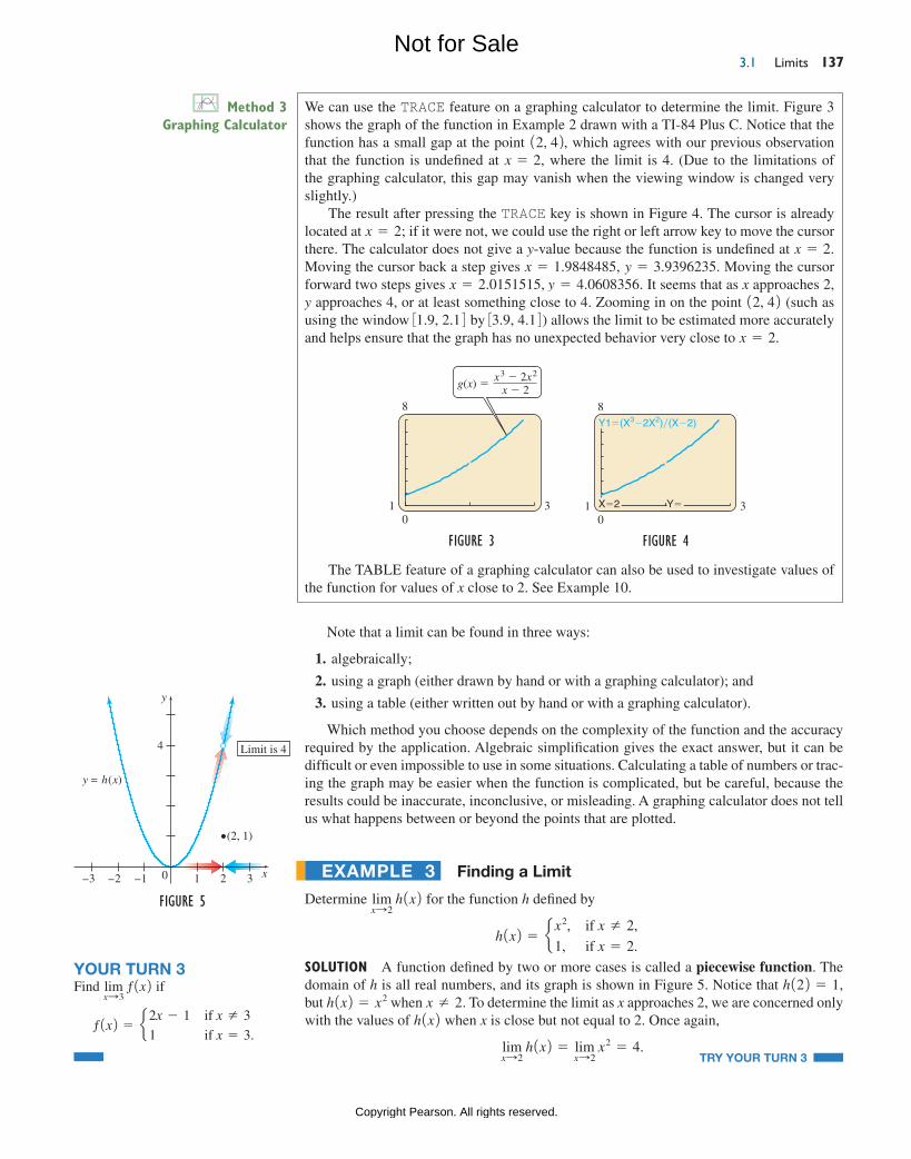
We can use the TRACE feature on a graphing calculator to determine the limit. Figure 3 shows the graph of the function in Example 2 drawn with a TI-84 Plus C. Notice that the function has a small gap at the point 12, 42, which agrees with our previous observation that the function is undefined at x = 2, where the limit is 4. (Due to the limitations of the graphing calculator, this gap may vanish when the viewing window is changed very slightly.)
The result after pressing the TRACE key is shown in Figure 4. The cursor is already located at x = 2; if it were not, we could use the right or left arrow key to move the cursor there. The calculator does not give a y-value because the function is undefined at x = 2. Moving the cursor back a step gives x = 1.9848485, y = 3.9396235. Moving the cursor forward two steps gives x = 2.0151515, y = 4.0608356. It seems that as x approaches 2, y approaches 4, or at least something close to 4. Zooming in on the point 12, 42 (such as using the window 31.9, 2.14 by 33.9, 4.14) allows the limit to be estimated more accurately and helps ensure that the graph has no unexpected behavior very close to x = 2.
Method 3 Graphing calculator
Figure 3
1 3
8
0
g(x) � x3 � 2x2
x � 2
Figure 4
1 3
8
0
Y1�(X3�2X2)�(X�2)Y1�(X3�2X2)�(X�2)
X�2 Y�
The TABLE feature of a graphing calculator can also be used to investigate values of the function for values of x close to 2. See Example 10.
YOUR TURN 3Find lim
xS3 ƒ1x2 if
ƒ1x2 = e2x - 1
1
if x Z 3
if x = 3.
Figure 5
y = h(x)
–3 –2 –1 2 310 x
y
4 Limit is 4
(2, 1)
M03_LIAL8774_11_AIE_C03_133-208.indd 137 23/06/15 11:30 AM
Not for Sale
Copyright Pearson. All rights reserved.
ChAptER 3 the Derivative 138
Finding a Limit
Find limxS-2
ƒ1x2, where
ƒ1x2 =3x + 2
2x + 4 .
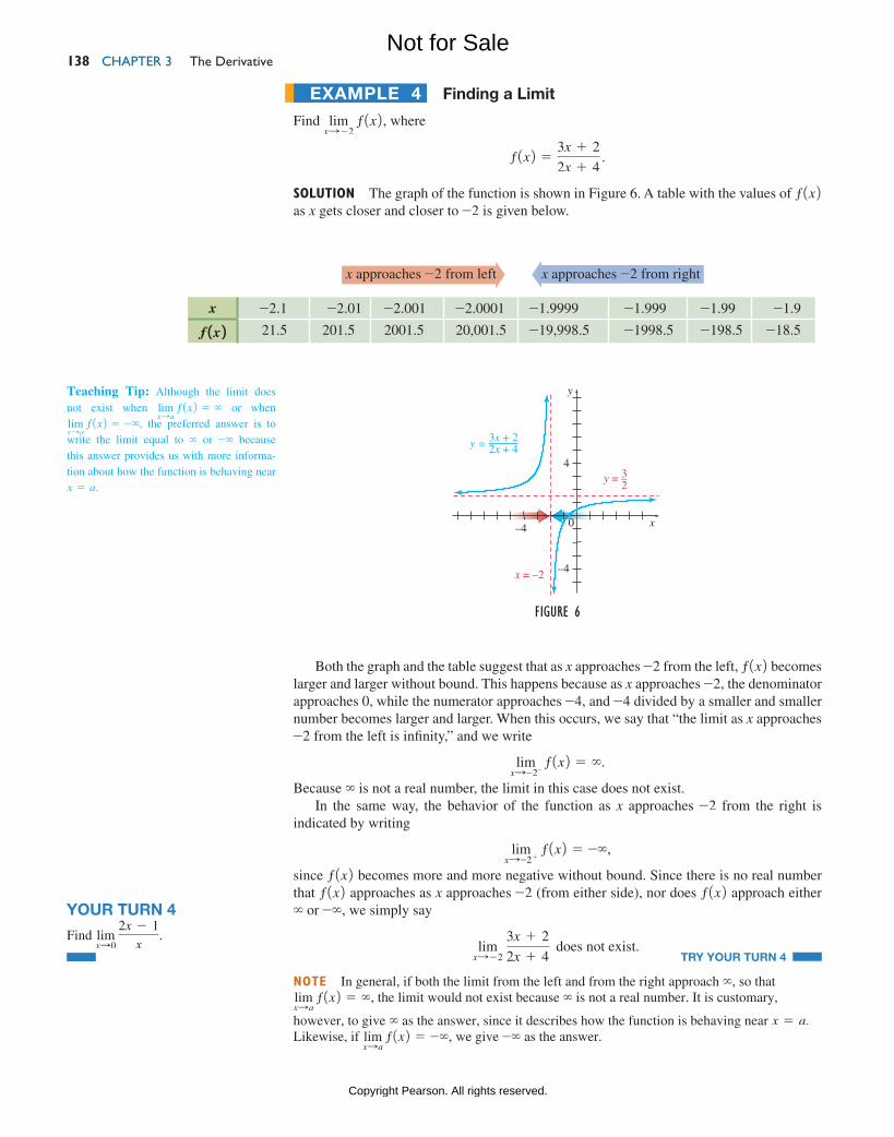
Solution The graph of the function is shown in Figure 6. A table with the values of ƒ1x2 as x gets closer and closer to -2 is given below.
ExampLE 4
x -2.1 -2.01 -2.001 -2.0001 -1.9999 -1.999 -1.99 -1.9
ƒ 1x 2 21.5 201.5 2001.5 20,001.5 -19,998.5 -1998.5 -198.5 -18.5
x approaches -2 from left x approaches -2 from right
Both the graph and the table suggest that as x approaches -2 from the left, ƒ1x2 becomes larger and larger without bound. This happens because as x approaches -2, the denominator approaches 0, while the numerator approaches -4, and -4 divided by a smaller and smaller number becomes larger and larger. When this occurs, we say that “the limit as x approaches -2 from the left is infinity,” and we write
limxS-2- ƒ1x2 = ∞.
Because ∞ is not a real number, the limit in this case does not exist.In the same way, the behavior of the function as x approaches -2 from the right is
indicated by writing
limxS-2 + ƒ1x2 = -∞,
since ƒ1x2 becomes more and more negative without bound. Since there is no real number that ƒ1x2 approaches as x approaches -2 (from either side), nor does ƒ1x2 approach either ∞ or -∞, we simply say
limxS-2
3x + 2
2x + 4 does not exist.
TRY YOUR TURN 4
note In general, if both the limit from the left and from the right approach ∞, so that limxSa
ƒ1x2 = ∞, the limit would not exist because ∞ is not a real number. It is customary,
however, to give ∞ as the answer, since it describes how the function is behaving near x = a. Likewise, if lim
xSa ƒ1x2 = -∞, we give -∞ as the answer.
YOUR TURN 4
Find limxS0
2x - 1
x.
Figure 6
y
x
x = –2 –4
4
–4 0
y = –32
3x + 22x + 4y =
Teaching Tip: Although the limit does not exist when lim
xSa ƒ1x2 = ∞ or when
limxSa
ƒ1x2 = -∞, the preferred answer is to write the limit equal to ∞ or -∞ because this answer provides us with more informa-tion about how the function is behaving near x = a.
M03_LIAL8774_11_AIE_C03_133-208.indd 138 23/06/15 11:30 AM
Not for Sale
Copyright Pearson. All rights reserved.
3.1 Limits 139
Finding a Limit
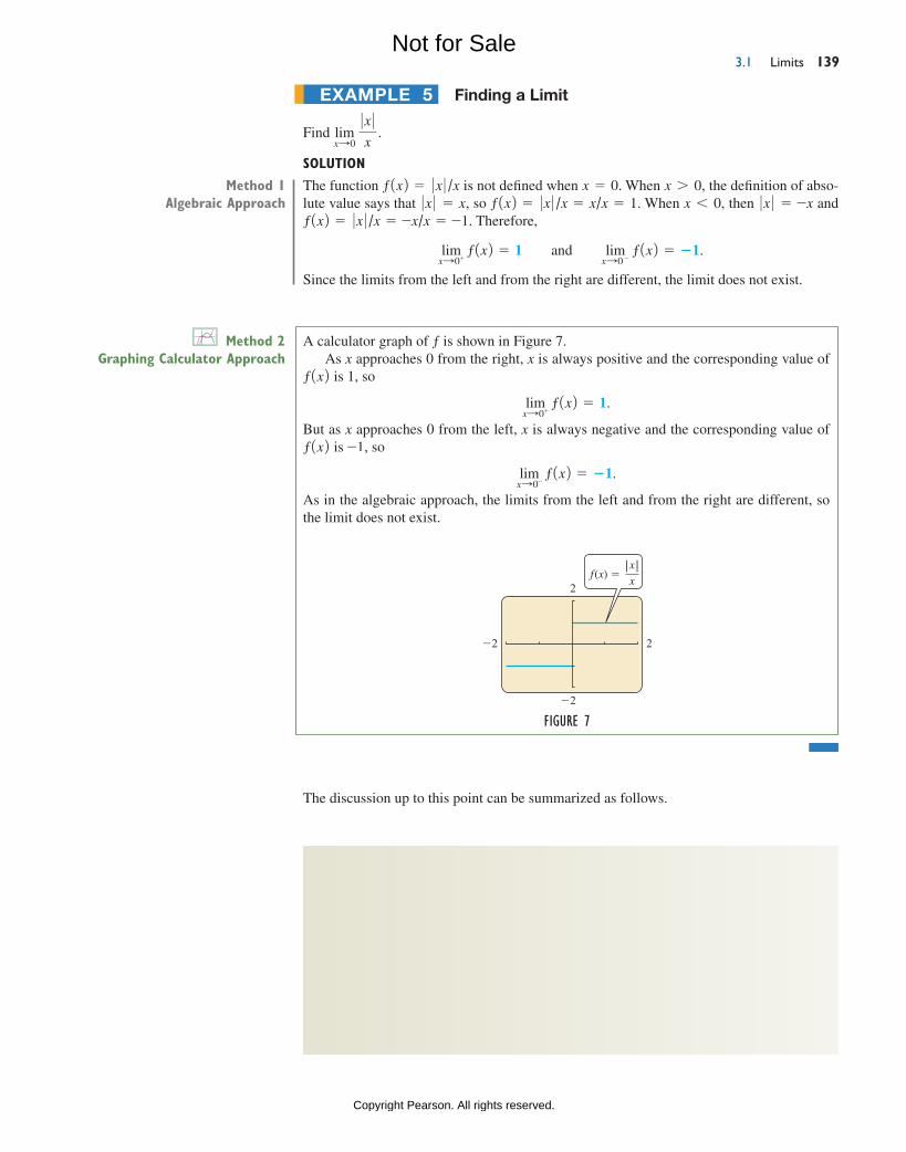
Find limxS0
0 x 0x
.
Solution
The function ƒ1x2 = 0 x 0 /x is not defined when x = 0. When x 7 0, the definition of abso-lute value says that 0 x 0 = x, so ƒ1x2 = 0 x 0 /x = x/x = 1. When x 6 0, then 0 x 0 = -x and ƒ1x2 = 0 x 0 /x = -x/x = -1. Therefore,
limxS0+ ƒ1x2 = 1 and lim
xS0 - ƒ1x2 = −1.
Since the limits from the left and from the right are different, the limit does not exist.
ExampLE 5
The discussion up to this point can be summarized as follows.
Method 1 Algebraic Approach
Method 2 Graphing Calculator Approach
Figure 7
�2 2
2
�2
f(x) �|x |x
A calculator graph of ƒ is shown in Figure 7.As x approaches 0 from the right, x is always positive and the corresponding value of
ƒ1x2 is 1, so
limxS0+ ƒ1x2 = 1.
But as x approaches 0 from the left, x is always negative and the corresponding value of ƒ1x2 is -1, so
limxS0- ƒ1x2 = −1.
As in the algebraic approach, the limits from the left and from the right are different, so the limit does not exist.
existence of LimitsThe limit of ƒ as x approaches a may not exist.
1. If ƒ1x2 becomes infinitely large in magnitude (positive or negative) as x approaches the number a from either side, we write lim
xSa ƒ1x2 = ∞ or lim
xSa ƒ1x2 = -∞. In either
case, the limit does not exist.
2. If ƒ1x2 becomes infinitely large in magnitude (positive) as x approaches a from one side and infinitely large in magnitude (negative) as x approaches a from the other side, then lim
xSa ƒ1x2 does not exist.
3. If limxSa- ƒ1x2 = L and lim
xSa+ ƒ1x2 = M, and L Z M, then limxSa
ƒ1x2 does not exist.
M03_LIAL8774_11_AIE_C03_133-208.indd 139 27/06/15 12:26 PM
Not for Sale
Copyright Pearson. All rights reserved.
ChAptER 3 the Derivative 140
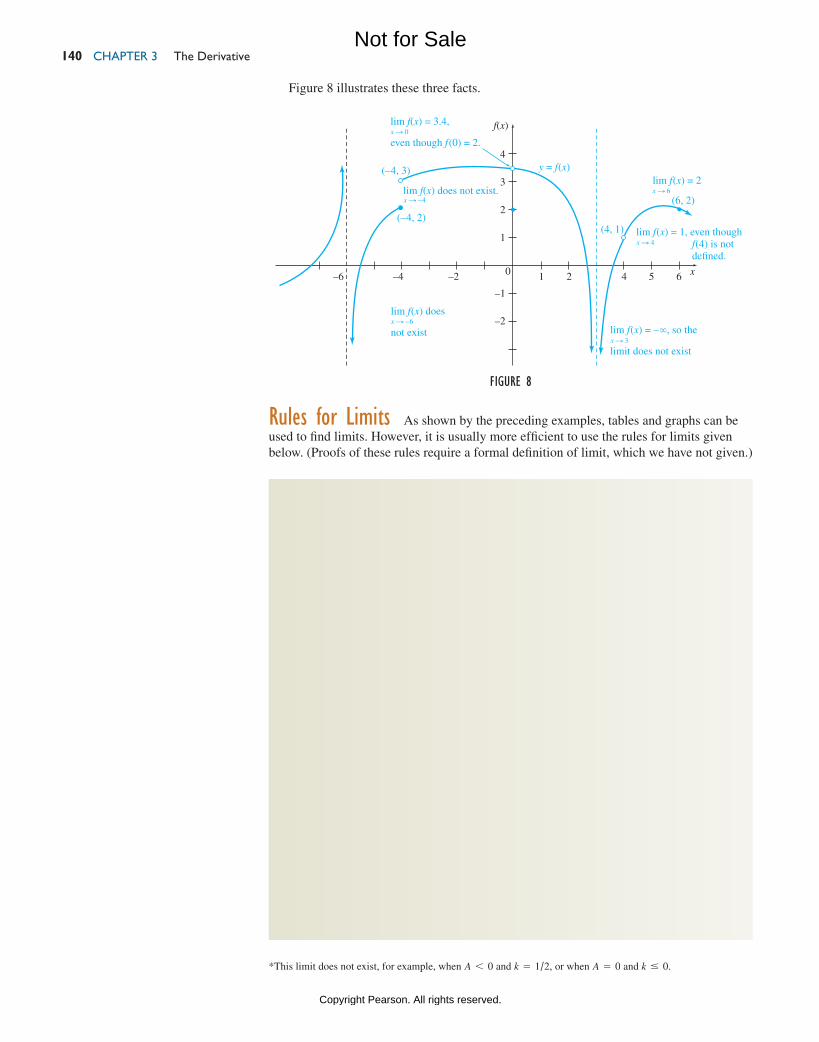
Figure 8 illustrates these three facts.
Figure 8
f(x)
x
y = f(x)
–1
1
2
3
4
–4–6 –2 10 2 4 5 6
–2
(–4, 3)
(–4, 2)
lim f(x) = 3.4,
even though f(0) = 2.
lim f(x) does
not exist lim f(x) = –∞, so the
limit does not exist
lim f(x) = 1, even though f(4) is not de�ned.
lim f(x) = 2
(6, 2)
(4, 1)
lim f(x) does not exist.
x S 0
x S –4
x S –6
x S 4
x S 6
x S 3
rules for Limits As shown by the preceding examples, tables and graphs can be used to find limits. However, it is usually more efficient to use the rules for limits given below. (Proofs of these rules require a formal definition of limit, which we have not given.)
*This limit does not exist, for example, when A 6 0 and k = 1/2, or when A = 0 and k … 0.
rules for LimitsLet a, A, and B be real numbers, and let ƒ and g be functions such that
limxSa
ƒ1x2 = A and limxSa
g1x2 = B.
1. If k is a constant, then limxSa
k = k and limxSa
[k # ƒ1x2] = k # limxSa
ƒ1x2 = k # A.
2. limxSa
3ƒ1x2 ± g1x24 = limxSa
ƒ1x2 ± limxSa
g1x2 = A ± B
(The limit of a sum or difference is the sum or difference of the limits.)
3. limxSa
3ƒ1x2 # g1x24 = 3limxSa
ƒ1x24 # 3limxSa
g1x24 = A # B
(The limit of a product is the product of the limits.)
4. limxSa
ƒ1x2g1x2 =
limxSa
ƒ1x2limxSa
g1x2=
A
B if B Z 0
(The limit of a quotient is the quotient of the limits, provided the limit of the denomi-nator is not zero.)
5. If p1x2 is a polynomial, then limxSa
p1x2 = p1a2.
6. For any real number k, limxSa
3 ƒ1x24 k = 3limxSa
ƒ1x24 k = Ak, provided this limit exists.*
7. limxSa
ƒ1x2 = limxSa
g1x2 if ƒ1x2 = g1x2 for all x Z a.
8. For any real number b 7 0, limxSa
bƒ1x2 = b3limxSa
ƒ1x24 = b A.
9. For any real number b such that 0 6 b 6 1 or 1 6 b,
limxSa
3log b
ƒ1x24 = logb 3limxSa
ƒ1x24 = logb A if A 7 0.
M03_LIAL8774_11_AIE_C03_133-208.indd 140 23/06/15 11:30 AM
Not for Sale
Copyright Pearson. All rights reserved.
3.1 Limits 141
This list may seem imposing, but these limit rules, once understood, agree with common sense. For example, Rule 3 says that if ƒ1x2 becomes close to A as x approaches a, and if g1x2 becomes close to B, then ƒ1x2 # g1x2 should become close to A # B, which seems plausible.
Rules for Limits
Suppose limxS2
ƒ1x2 = 3 and limxS2
g1x2 = 4. Use the limit rules to find the following limits.
(a) limxS2
3ƒ1x2 + 5g1x24Solution
limxS2
3 ƒ1x2 + 5g1x24 = limxS2
ƒ1x2 + limxS2
5g1x2 Rule 2
= limxS2
ƒ1x2 + 5 limxS2
g1x2 Rule 1
= 3 + 5142
= 23
(b) limxS2
3 ƒ1x242ln g1x2
Solution
limxS2
3ƒ1x24
2
ln g1x2 =limxS2
3ƒ1x24
2
limxS2
ln g1x2 Rule 4
=3limxS2
ƒ1x24
2
ln3limxS2
g1x24 Rule 6 and Rule 9
=32
ln 4
≈9
1.38629≈ 6.492
TRY YOUR TURN 5
Finding a Limit
Find limxS3
x2 - x - 11x + 1
.
Solution
limxS3
x2 - x - 11x + 1
=limxS3
1x2 - x - 12limxS3
1x + 1 Rule 4
=limxS3
1x2 - x - 122limxS3
1x + 12 Rule 6 11a = a1/2 2
=32 - 3 - 113 + 1
Rule 5
=514
=5
2
As Examples 6 and 7 suggest, the rules for limits actually mean that many limits can be found simply by evaluation. This process is valid for polynomials, rational functions, exponential functions, logarithmic functions, and roots and powers, as long as this does
ExampLE 6
ExampLE 7
YOUR TURN 5Find lim
xS2 3 ƒ1x2 + g1x242.
M03_LIAL8774_11_AIE_C03_133-208.indd 141 23/06/15 11:31 AM
Not for Sale
Copyright Pearson. All rights reserved.
ChAptER 3 the Derivative 142
not involve an illegal operation, such as division by 0 or taking the logarithm of a negative number. Division by 0 presents particular problems that can often be solved by algebraic simplification, as the following example shows.
Finding a Limit
Find limxS2
x2 + x - 6
x - 2 .
Solution Rule 4 cannot be used here, since
limxS21x - 22 = 0.
The numerator also approaches 0 as x approaches 2, and 0/0 is meaningless. For x Z 2, we can, however, simplify the function by rewriting the fraction as
x2 + x - 6
x - 2=1x + 321x - 22
x - 2= x + 3.
Now Rule 7 can be used.
limxS2
x2 + x - 6
x - 2= lim
xS21x + 32 = 2 + 3 = 5
TRY YOUR TURN 6
note Mathematicians often refer to a limit that gives 0/0, as in Example 8, as an indeter-minate form. This means that when the numerator and denominator are polynomials, they must have a common factor, which is why we factored the numerator in Example 8.
Finding a Limit
Find limxS4
1x - 2
x - 4 .
Solution
As x S 4, the numerator approaches 0 and the denominator also approaches 0, giving the meaningless expression 0/0. In an expression such as this involving square roots, rather than trying to factor, you may find it simpler to use algebra to rationalize the numerator by multiplying both the numerator and the denominator by 2x + 2. This gives
1x - 2
x - 4# 1x + 21x + 2
=11x22 - 22
1x - 4211x + 22 1a − b 2 1a + b 2 = a2 − b2
=x - 4
1x - 4211x + 22 =11x + 2
if x Z 4. Now use the rules for limits.
limxS4
1x - 2
x - 4= lim
xS4
11x + 2=
114 + 2=
1
2 + 2=
1
4
Alternatively, we can take advantage of the fact that x - 4 = 12x22 - 22 =12x + 2212x - 22 because of the factoring a2 - b2 = 1a + b21a - b2. Then
limxS4
2x - 2
x - 4= lim
xS4
2x - 2
12x + 2212x - 22
= lim xS4
12x + 2
=124 + 2
=1
2 + 2=
1
4 .
TRY YOUR TURN 7
ExampLE 8
ExampLE 9
YOUR TURN 6 Find
limxS-3
x2 - x - 12
x + 3 .
YOUR TURN 7
Find limxS1
1x - 1
x - 1 .
Method 1 Rationalizing the numerator
Method 2 Factoring
M03_LIAL8774_11_AIE_C03_133-208.indd 142 23/06/15 11:31 AM
Not for Sale
Copyright Pearson. All rights reserved.
3.1 Limits 143
Simply because the expression in a limit is approaching 0/0, as in Examples 8 and 9, does not mean that the limit is 0 or that the limit does not exist. For such a limit, try to simplify the expression using the following principle: To calculate the limit of ƒ 1x 2 /g 1x 2 as x approaches a, where ƒ 1a 2 = g 1a 2 = 0, you should attempt to factor x − a from both the numerator and the denominator.
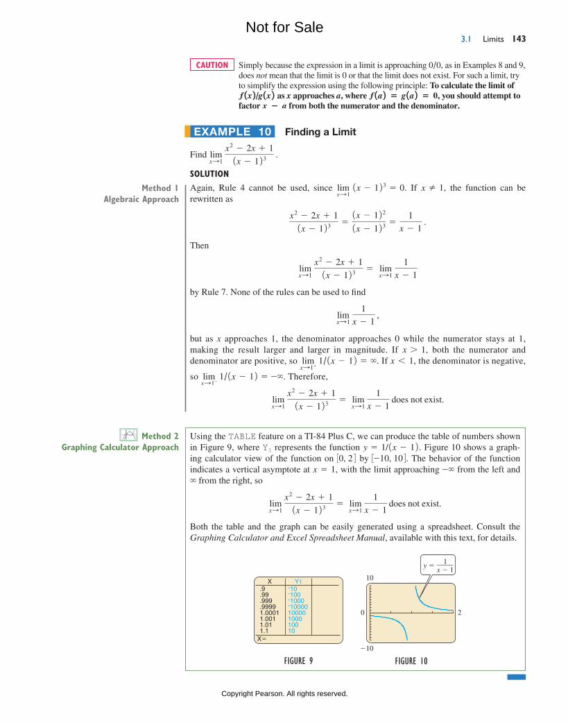
Finding a Limit
Find limxS1
x2 - 2x + 11x - 123 .
Solution
Again, Rule 4 cannot be used, since limxS1
1x - 123 = 0. If x Z 1, the function can be rewritten as
x2 - 2x + 11x - 123 =
1x - 122
1x - 123 =1
x - 1 .
Then
limxS1
x2 - 2x + 11x - 123 = lim
xS1
1
x - 1
by Rule 7. None of the rules can be used to find
limxS1
1
x - 1 ,
but as x approaches 1, the denominator approaches 0 while the numerator stays at 1, making the result larger and larger in magnitude. If x 7 1, both the numerator and denominator are positive, so lim
xS1+ 1/1x - 12 = ∞. If x 6 1, the denominator is negative,
so limxS1-
1/1x - 12 = -∞. Therefore,
limxS1
x2 - 2x + 11x - 123 = lim
xS1
1
x - 1 does not exist.
caution
ExampLE 10
Method 2 Graphing calculator approach
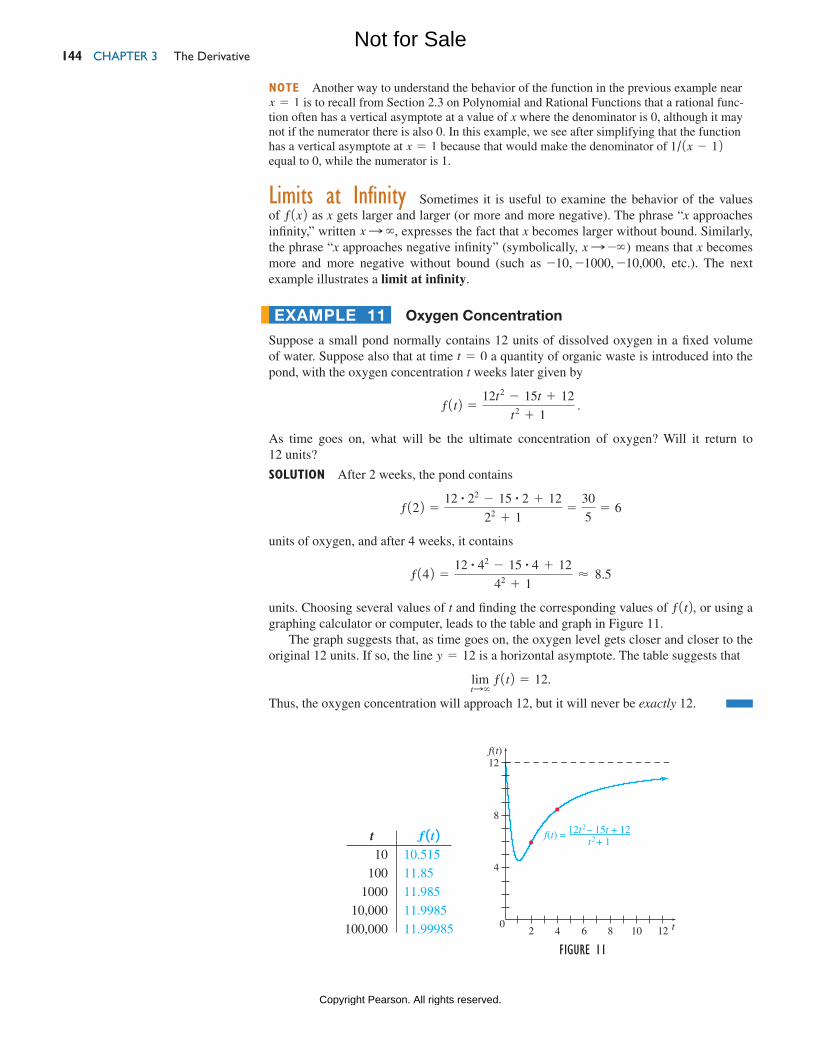
Using the TABLE feature on a TI-84 Plus C, we can produce the table of numbers shown in Figure 9, where Y1 represents the function y = 1/1x - 12. Figure 10 shows a graph-ing calculator view of the function on 30, 24 by 3-10, 104. The behavior of the function indicates a vertical asymptote at x = 1, with the limit approaching -∞ from the left and ∞ from the right, so
limxS1
x2 - 2x + 11x - 123 = lim
xS1
1
x - 1 does not exist.
Both the table and the graph can be easily generated using a spreadsheet. Consult the Graphing Calculator and Excel Spreadsheet Manual, available with this text, for details.
Figure 9
.9
.99
.999
.99991.00011.0011.01
-10-100-1000-1000010000100010010
Y1-10-100-1000-1000010000100010010
X�
X Y1
1.1
Figure 10
0 2
10
�10
y �1
x � 1
Method 1 algebraic approach
M03_LIAL8774_11_AIE_C03_133-208.indd 143 23/06/15 11:31 AM
Not for Sale
Copyright Pearson. All rights reserved.
ChAptER 3 the Derivative 144
note Another way to understand the behavior of the function in the previous example near x = 1 is to recall from Section 2.3 on Polynomial and Rational Functions that a rational func-tion often has a vertical asymptote at a value of x where the denominator is 0, although it may not if the numerator there is also 0. In this example, we see after simplifying that the function has a vertical asymptote at x = 1 because that would make the denominator of 1/1x - 12 equal to 0, while the numerator is 1.
Limits at infinity Sometimes it is useful to examine the behavior of the values of ƒ1x2 as x gets larger and larger (or more and more negative). The phrase “x approaches infinity,” written x S ∞, expresses the fact that x becomes larger without bound. Similarly, the phrase “x approaches negative infinity” (symbolically, x S -∞) means that x becomes more and more negative without bound (such as -10, -1000, -10,000, etc.). The next example illustrates a limit at infinity.
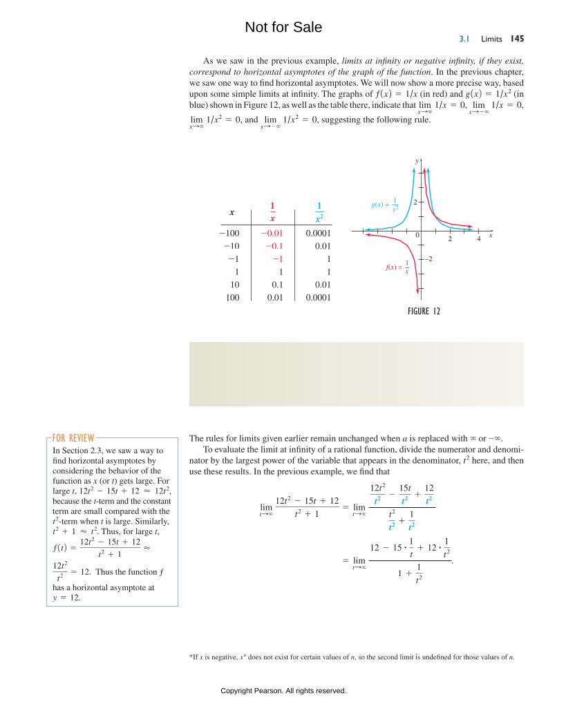
Oxygen Concentration
Suppose a small pond normally contains 12 units of dissolved oxygen in a fixed volume of water. Suppose also that at time t = 0 a quantity of organic waste is introduced into the pond, with the oxygen concentration t weeks later given by
ƒ1t2 =12t2 - 15t + 12
t2 + 1 .
As time goes on, what will be the ultimate concentration of oxygen? Will it return to 12 units?
Solution After 2 weeks, the pond contains
ƒ122 =12 # 22 - 15 # 2 + 12
22 + 1=
30
5= 6
units of oxygen, and after 4 weeks, it contains
ƒ142 =12 # 42 - 15 # 4 + 12
42 + 1≈ 8.5
units. Choosing several values of t and finding the corresponding values of ƒ1t2, or using a graphing calculator or computer, leads to the table and graph in Figure 11.
The graph suggests that, as time goes on, the oxygen level gets closer and closer to the original 12 units. If so, the line y = 12 is a horizontal asymptote. The table suggests that
limtS∞
ƒ1t2 = 12.
Thus, the oxygen concentration will approach 12, but it will never be exactly 12.
ExampLE 11
Figure 11
12
8
4
20
4 6 10 128
f(t)
t
212t – 15t + 12t + 1
f(t) = 2 t ƒ 1 t 2 10 10.515
100 11.85
1000 11.985
10,000 11.9985
100,000 11.99985
M03_LIAL8774_11_AIE_C03_133-208.indd 144 23/06/15 11:31 AM
Not for Sale
Copyright Pearson. All rights reserved.
3.1 Limits 145
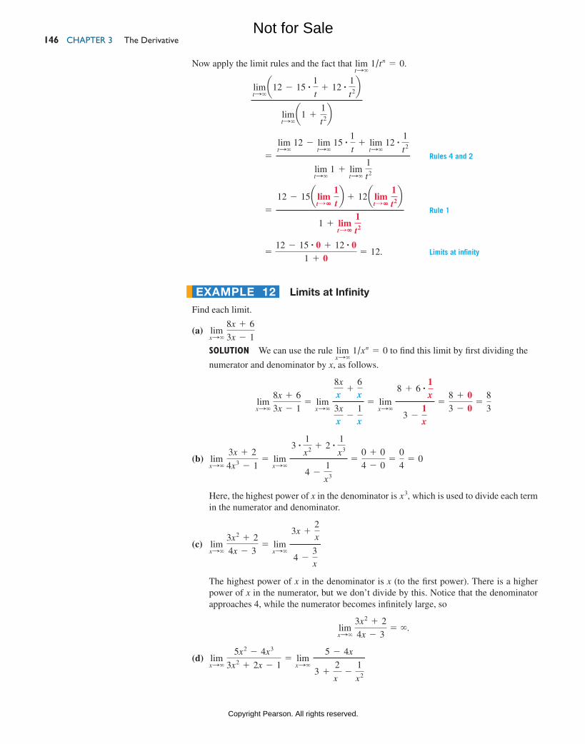
As we saw in the previous example, limits at infinity or negative infinity, if they exist, correspond to horizontal asymptotes of the graph of the function. In the previous chapter, we saw one way to find horizontal asymptotes. We will now show a more precise way, based upon some simple limits at infinity. The graphs of ƒ1x2 = 1/x (in red) and g1x2 = 1/x2 (in blue) shown in Figure 12, as well as the table there, indicate that lim
xS∞ 1/x = 0, lim
xS-∞ 1/x = 0,
limxS∞
1/x2 = 0, and limxS-∞
1/x2 = 0, suggesting the following rule.
*If x is negative, xn does not exist for certain values of n, so the second limit is undefined for those values of n.
Limits at infinityFor any positive real number n,
limxSH
1xn = 0 and lim
xS−H 1xn = 0.*
The rules for limits given earlier remain unchanged when a is replaced with ∞ or -∞.To evaluate the limit at infinity of a rational function, divide the numerator and denomi-
nator by the largest power of the variable that appears in the denominator, t2 here, and then use these results. In the previous example, we find that
limtS∞
12t2 - 15t + 12
t2 + 1= lim
tS∞
12t2
t2 -15t
t2 +12
t2
t2
t2 +1
t2
= limtS∞
12 - 15 # 1
t+ 12 # 1
t2
1 +1
t2
.
For reviewIn Section 2.3, we saw a way to find horizontal asymptotes by considering the behavior of the function as x (or t) gets large. For large t, 12t2 - 15t + 12 ≈ 12t2, because the t-term and the constant term are small compared with the t2-term when t is large. Similarly, t2 + 1 ≈ t2. Thus, for large t,
ƒ1t2 =12t2 - 15t + 12
t2 + 1 ≈
12t2
t2 = 12. Thus the function ƒ
has a horizontal asymptote at y = 12.
Figure 12
0 2 4
–2
y
x
f(x) = 1x
2g(x) = 1x
2
x 1x
1
x2
-100 -0.01 0.0001
-10 -0.1 0.01
-1 -1 1
1 1 1
10 0.1 0.01
100 0.01 0.0001
M03_LIAL8774_11_AIE_C03_133-208.indd 145 23/06/15 11:31 AM
Not for Sale
Copyright Pearson. All rights reserved.
ChAptER 3 the Derivative 146
Now apply the limit rules and the fact that limtS∞
1/tn = 0.
limtS∞a12 - 15 # 1
t+ 12 # 1
t2b
limtS∞a1 +
1
t2b
=limtS∞
12 - limtS∞
15 # 1
t+ lim
tS∞ 12 # 1
t2
limtS∞
1 + limtS∞
1
t2
Rules 4 and 2
=12 - 15a lim
tSH 1tb + 12a lim
tSH 1
t2b
1 + limtSH
1
t2
Rule 1
=12 - 15 # 0 + 12 # 0
1 + 0= 12. Limits at infinity
Limits at Infinity
Find each limit.
(a) limxS∞
8x + 6
3x - 1
Solution We can use the rule limxS∞
1/xn = 0 to find this limit by first dividing the
numerator and denominator by x, as follows.
limxS∞
8x + 6
3x - 1= lim
xS∞
8xx
+6x
3xx
-1x
= limxS∞
8 + 6 # 1x
3 -1x
=8 + 03 - 0
=8
3
(b) limxS∞
3x + 2
4x3 - 1= lim
xS∞
3 # 1
x2 + 2 # 1
x3
4 -1
x3
=0 + 0
4 - 0=
0
4= 0
Here, the highest power of x in the denominator is x3, which is used to divide each term in the numerator and denominator.
(c) limxS∞
3x2 + 2
4x - 3= lim
xS∞
3x +2x
4 -3x
The highest power of x in the denominator is x (to the first power). There is a higher power of x in the numerator, but we don’t divide by this. Notice that the denominator approaches 4, while the numerator becomes infinitely large, so
limxS∞
3x2 + 2
4x - 3= ∞.
(d) limxS∞
5x2 - 4x3
3x2 + 2x - 1= lim
xS∞
5 - 4x
3 +2
x-
1
x2
ExampLE 12
M03_LIAL8774_11_AIE_C03_133-208.indd 146 23/06/15 11:31 AM
Not for Sale
Copyright Pearson. All rights reserved.
3.1 Limits 147
The highest power of x in the denominator is x2. The denominator approaches 3, while the numerator becomes a negative number that is larger and larger in magnitude, so
limxS∞
5x2 - 4x3
3x2 + 2x - 1= -∞.
TRY YOUR TURN 8
The method used in Example 12 is a useful way to rewrite expressions with fractions so that the rules for limits at infinity can be used.
Finding Limits at infinityIf ƒ1x2 = p1x2/q1x2, for polynomials p1x2 and q1x2, q1x2 Z 0, lim
xS-∞ ƒ1x2 and lim
xS∞ ƒ1x2
can be found as follows.
1. Divide p1x2 and q1x2 by the highest power of x in q1x2. 2. Use the rules for limits, including the rules for limits at infinity,
limxSH
1xn = 0 and lim
xS−H 1xn = 0,
to find the limit of the result from Step 1.
For an alternate approach to finding limits at infinity, see Exercise 83.
YOUR TURN 8 Find
limxS∞
2x2 + 3x - 4
6x2 - 5x + 7 .
Teaching Tip: Students will have the best understanding of limits if they have studied them graphically (as in Exercises 5–12), numerically (as in Exercises 15–20), and analytically (as in Exercises 31–52).
3.1 exercisesIn Exercises 1–4, choose the best answer for each limit.
1. If limxS2-
ƒ1x2 = 5 and limxS2+
ƒ1x2 = 6, then limxS2
ƒ1x2 (c)
(a) is 5. (b) is 6.
(c) does not exist. (d) is infinite.
2. If limxS2-
ƒ1x2 = limxS2+
ƒ1x2 = -1, but ƒ122 = 1, then limxS2
ƒ1x2 (a)
(a) is -1. (b) does not exist.
(c) is infinite. (d) is 1.
3. If limxS4-
ƒ1x2 = limxS4+
ƒ1x2 = 6, but ƒ142 does not exist, then
limxS4
ƒ1x2 (b)
(a) does not exist. (b) is 6.
(c) is -∞. (d) is ∞.
4. If limxS1-
ƒ1x2 = -∞ and limxS1+
ƒ1x2 = -∞, then limxS1
ƒ1x2 (b)
(a) is ∞. (b) is -∞.
(c) does not exist. (d) is 1.
Factor each of the following expressions. (Sec. R.2)3.1 warm-up exercises
W1. 8x2 + 22x + 15 12x + 3214x + 52
W4. 2x2 + x - 15
x2 - 9 12x - 52/1x - 32
W2. 12x2 - 7x - 12 13x - 4214x + 32Simplify each of the following expressions. (Sec. R.3)
W3. 3x2 + x - 14
x2 - 4 13x + 72/1x + 22
M03_LIAL8774_11_AIE_C03_133-208.indd 147 23/06/15 11:31 AM
Not for Sale
Copyright Pearson. All rights reserved.
ChAptER 3 the Derivative 148
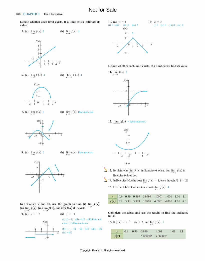
Decide whether each limit exists. If a limit exists, estimate its value.
5. (a) limxS3
ƒ1x2 3 (b) limxS0
ƒ1x2 1
10. (a) a = 1 (b) a = 2
0 21
–2
3 4
f (x)
x
4
3
2
1
0 21–1–2 3
F(x)
x
4
2
6. (a) limxS2
F 1x2 4 (b) limxS-1
F 1x2 4
7. (a) limxS0
ƒ1x2 0 (b) limxS2
ƒ1x2 Does not exist
8. (a) limxS3
g1x2 2 (b) limxS5
g1x2 Does not exist
–3
f(x)
2–4 –2 x
3
0
0 3–2–2
g(x)
x
2
In Exercises 9 and 10, use the graph to find (i) limxSa−
ƒ 1x 2 , (ii) lim
xSa+ ƒ 1x 2 , (iii) lim
xSa ƒ 1x 2 , and (iv) ƒ 1a 2 if it exists.
9. (a) a = -2 (b) a = -1
(a) (i) -1; (ii) -1/2 (iii) Does not exist; (iv) Does not exist
(b) (i) -1/2 (ii) -1/2 (iii) -1/2 (iv) -1/20
f(x)1
–1
–2 –1 1
x
(i) 1 (ii) 1 (iii) 1 (iv) 2 (i) 0 (ii) 0 (iii) 0 (iv) 0
0
f(x)
1
–2
2
–2 1 2 3 x
Decide whether each limit exists. If a limit exists, find its value.
11. limxS∞
ƒ1x2 3
12. limxS-∞
g1x2 ∞ (does not exist)
0
f(x)
3
–2 4 x
0
g(x)
3
–3
6
–2 4 x
13. Explain why limxS2
F 1x2 in Exercise 6 exists, but limxS-2
ƒ1x2 in
Exercise 9 does not.
14. In Exercise 10, why does limxS1
ƒ1x2 = 1, even though ƒ112 = 2?
15. Use the table of values to estimate limxS1
ƒ1x2. 4
x 0.9 0.99 0.999 0.9999 1.0001 1.001 1.01 1.1
ƒ 1x 2 3.9 3.99 3.999 3.9999 4.0001 4.001 4.01 4.1
Complete the tables and use the results to find the indicated limits.
16. If ƒ1x2 = 2x2 - 4x + 7, find limxS1
ƒ1x2. 5
x 0.9 0.99 0.999 1.001 1.01 1.1
ƒ 1x 2 5.000002 5.000002
M03_LIAL8774_11_AIE_C03_133-208.indd 148 23/06/15 11:31 AM
Not for Sale
Copyright Pearson. All rights reserved.
3.1 Limits 149
17. If k1x2 =x3 - 2x - 4
x - 2 , find lim
xS2 k1x2. 10
x 1.9 1.99 1.999 2.001 2.01 2.1
k 1x 2
18. If ƒ1x2 =2x3 + 3x2 - 4x - 5
x + 1 , find lim
xS-1 ƒ1x2. -4
x -1.1 -1.01 -1.001 -0.999 -0.99 -0.9
ƒ 1x 2
19. If h1x2 =2x - 2
x - 1 , find lim
xS1 h1x2. Does not exist
x 0.9 0.99 0.999 1.001 1.01 1.1
h 1x 2
20. If ƒ1x2 =2x - 3
x - 3 , find lim
xS3 ƒ1x2. Does not exist
x 2.9 2.99 2.999 3.001 3.01 3.1
ƒ 1x 2
Let limxS4
ƒ 1x 2 = 9 and limxS4
g 1x 2 = 27. Use the limit rules to find
each limit.
53. Let ƒ1x2 = e x3 + 2
5
if x Z -1
if x = -1. Find lim
xS-1 ƒ1x2. 1
54. Let g1x2 = e012 x
2 - 3
if x = -2
if x Z -2. Find lim
xS-2 g1x2. -1
55. Let ƒ1x2 = •x - 1
2
x + 3
if x 6 3
if 3 … x … 5 .
if x 7 5
(a) Find limxS3
ƒ1x2. 2 (b) Find limxS5
ƒ1x2.
56. Let g1x2 = •5
x2 - 2
7
if x 6 0
if 0 … x … 3 .
if x 7 3
(a) Find limxS0
g1x2. (b) Find limxS3
g1x2. 7
57. Does a value of k exist such that the following limit exists?
limxS2
3x2 + kx - 2
x2 - 3x + 2
If so, find the value of k and the corresponding limit. If not, explain why not. -5, 7
58. Repeat the instructions of Exercise 57 for the following limit.
limxS3
2x2 + kx - 9
x2 - 4x + 3
In Exercises 59–62, calculate the limit in the specified exercise, using a table such as in Exercises 15–20. Verify your answer by using a graphing calculator to zoom in on the point on the graph.
21. limxS4
3ƒ1x2 - g1x24 -18 22. limxS4
3 g1x2 # ƒ1x24 243
23. limxS4
ƒ1x2g1x2 1/3
24. lim
xS4 log3 ƒ1x2 2
25. limxS4
2ƒ1x2 3 26. limxS4
23 g1x2 3
27. limxS4
2ƒ1x2 512 28. limxS4
31 + ƒ1x242 100
29. limxS4
ƒ1x2 + g1x2
2g1x2 2/3 30. limxS4
5g1x2 + 2
1 - ƒ1x2 -137/8
59. Exercise 31 6 60. Exercise 32 -4
61. Exercise 33 1.5 62. Exercise 34 1.2
45. limxS-∞
3x2 + 2x
2x2 - 2x + 1 3/2 46. lim
xS∞ x2 + 2x - 5
3x2 + 2 1/3
49. limxS∞
2x3 - x - 3
6x2 - x - 1 50. lim
xS∞ x4 - x3 - 3x
7x2 + 9
39. limxS25
1x - 5
x - 25 1/10 40. lim
xS36 1x - 6
x - 36 1/12
31. limxS3
x2 - 9
x - 3 6 32. lim
xS-2 x2 - 4
x + 2 -4
35. limxS-2
x2 - x - 6
x + 2 -5 36. lim
xS5 x2 - 3x - 10
x - 5 7
63. Let F1x2 =3x
1x + 223 .
(a) Find limxS-2
F1x2. Does not exist
(b) Find the vertical asymptote of the graph of F1x2. x = -2
(c) Compare your answers for parts (a) and (b). What can you conclude?
64. Let G1x2 =-6
1x - 422 .
(a) Find limxS4
G1x2. -∞ (does not exist)
(b) Find the vertical asymptote of the graph of G1x2. x = 4
(c) Compare your answers for parts (a) and (b). Are they related? How?
47. limxS∞
3x3 + 2x - 1
2x4 - 3x3 - 2 0 48. lim
xS∞ 2x2 - 1
3x4 + 2 0
51. limxS∞
2x2 - 7x4
9x2 + 5x - 6 52. lim
xS∞ -5x3 - 4x2 + 8
6x2 + 3x + 2
41. limhS0
1x + h22 - x2
h 2x 42. lim
hS0 1x + h23 - x3
h 3x2
43. limxS∞
3x
7x - 1 3/7 44. lim
xS-∞ 8x + 2
4x - 5 2
33. limxS1
5x2 - 7x + 2
x2 - 1 3/2 34. lim
xS-3
x2 - 9
x2 + x - 6 6/5
37. limxS0
1/1x + 32 - 1/3
x -1/9 38. lim
xS0 -1/1x + 22 + 1/2
x 1/4
Use the properties of limits to help decide whether each limit exists. If a limit exists, find its value.
∞ (does not exist) ∞ (does not exist)
-∞ (does not exist) -∞ (does not exist)
Does not exist
Does not exist
-3, 9/2
If x = a is a vertical asymptote for the graph of ƒ1x2, then lim
xSa ƒ1x2 does not exist.
If x = a is a vertical asymptote, then limxSa
ƒ1x2 does not exist
M03_LIAL8774_11_AIE_C03_133-208.indd 149 23/06/15 11:31 AM
Not for Sale
Copyright Pearson. All rights reserved.
ChAptER 3 the Derivative 150
65. Describe how the behavior of the graph in Figure 10 near x = 1 can be predicted by the simplified expression for the function y = 1/1x - 12.
66. A friend who is confused about limits wonders why you investi-gate the value of a function closer and closer to a point, instead of just finding the value of a function at the point. How would you respond?
67. Use a graph of ƒ1x2 = ex to answer the following questions.
(a) Find limxS-∞
ex. 0
(b) Where does the function ex have a horizontal asymptote?
68. Use a graphing calculator to answer the following questions.
(a) From a graph of y = xe-x, what do you think is the value of lim
xS∞ xe-x? Support this by evaluating the function for
several large values of x. 0
(b) Repeat part (a), this time using the graph of y = x2e-x . 0
(c) Based on your results from parts (a) and (b), what do you think is the value of lim
xS∞ xne-x, where n is a positive
integer? Support this by experimenting with other positive integers n. 0
69. Use a graph of ƒ1x2 = ln x to answer the following questions.
(a) Find limxS0+
ln x. -∞ (does not exist)
(b) Where does the function ln x have a vertical asymptote?
70. Use a graphing calculator to answer the following questions.
(a) From a graph of y = x ln x, what do you think is the value of lim
xS0+ x ln x? Support this by evaluating the function for
several small values of x. 0
(b) Repeat part (a), this time using the graph of y = x1ln x22. 0
(c) Based on your results from parts (a) and (b), what do you think is the value of lim
xS0+ x1ln x2n, where n is a positive integer?
Support this by experimenting with other positive integers n.
71. Explain in your own words why the rules for limits at infinity should be true.
72. Explain in your own words what Rule 4 for limits means.
Find each of the following limits (a) by investigating values of the function near the x-value where the limit is taken, and (b) using a graphing calculator to view the function near that value of x.
83. Explain why the following rules can be used to find limxS∞
3 p1x2/q1x24:(a) If the degree of p1x2 is less than the degree of q1x2, the
limit is 0.
(b) If the degree of p1x2 is equal to the degree of q1x2, the limit is A/B, where A and B are the leading coefficients of p1x2 and q1x2, respectively.
(c) If the degree of p1x2 is greater than the degree of q1x2, the limit is ∞ or -∞.
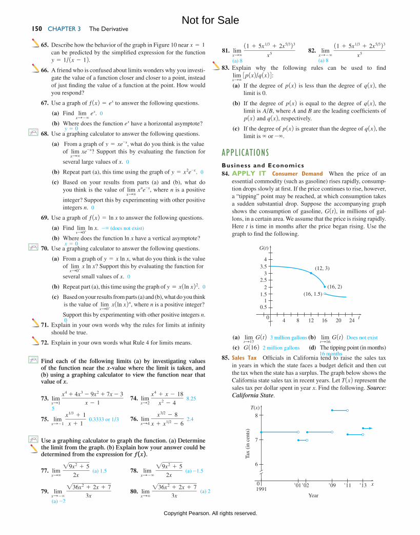
appLicationsBusiness and Economics 84. APPLY IT consumer Demand When the price of an
essential commodity (such as gasoline) rises rapidly, consump-tion drops slowly at first. If the price continues to rise, however, a “tipping” point may be reached, at which consumption takes a sudden substantial drop. Suppose the accompanying graph shows the consumption of gasoline, G1t2, in millions of gal-lons, in a certain area. We assume that the price is rising rapidly. Here t is time in months after the price began rising. Use the graph to find the following.
81. limxS∞
11 + 5x1/3 + 2x5/323
x5 82. limxS- ∞
11 + 5x1/3 + 2x5/323
x5
77. limxS∞
29x2 + 5
2x (a) 1.5 78. lim
xS-∞ 29x2 + 5
2x (a) -1.5
79. limxS-∞
236x2 + 2x + 7
3x 80. lim
xS∞ 236x2 + 2x + 7
3x
73. limxS1
x4 + 4x3 - 9x2 + 7x - 3
x - 1
y = 0
x = 0
0
5
74. limxS2
x4 + x - 18
x2 - 4 8.25
75. limxS-1
x1/3 + 1
x + 1 0.3333 or 1/3 76. lim
xS4
x3/2 - 8
x + x1/2 - 6 2.4
Use a graphing calculator to graph the function. (a) Determine the limit from the graph. (b) Explain how your answer could be determined from the expression for ƒ 1x 2 .
(a) -2
(a) 2
(a) 8 (a) 8
0 4 168 12 20 24t
G(t)
3.5
2.5
4
3
21.5
10.5
(12, 3)
(16, 2)(16, 1.5)
16 months
(a) limtS12
G1t2 3 million gallons (b) limtS16
G1t2 Does not exist
(c) G1162 2 million gallons (d) The tipping point (in months)
85. Sales tax Officials in California tend to raise the sales tax in years in which the state faces a budget deficit and then cut the tax when the state has a surplus. The graph below shows the California state sales tax in recent years. Let T1x2 represent the sales tax per dollar spent in year x. Find the following. Source: California State.
7
8
6
1991’01 ’09’02 x
T(x)
’11 ’130
Year
Tax
(in
cent
s)
M03_LIAL8774_11_AIE_C03_133-208.indd 150 23/06/15 11:31 AM
Not for Sale
Copyright Pearson. All rights reserved.
3.1 Limits 151
a perpetuity, receive payments that take the form of an annu-ity in that the amount of the payment never changes. However, normally the payments for preferred stock do not end but theo-retically continue forever. Find the limit of this present value equation as n approaches infinity to derive a formula for the present value of a share of preferred stock paying a periodic dividend R. Source: Robert D. Campbell. R/i
91. Growing Annuities For some annuities encountered in busi-ness finance, called growing annuities, the amount of the peri-odic payment is not constant but grows at a constant periodic rate. Leases with escalation clauses can be examples of growing annuities. The present value of a growing annuity takes the form
P =R
i - g c 1 - a1 + g
1 + ib
n
d ,
where
R = amount of the next annuity payment,
g = expected constant annuity growth rate,
i = required periodic return at the time the annuity is evaluated,
n = number of periodic payments.
A corporation’s common stock may be thought of as a claim on a growing annuity where the annuity is the company’s annual dividend. However, in the case of common stock, these payments have no contractual end but theoretically continue forever. Com-pute the limit of the expression above as n approaches infinity to derive the Gordon–Shapiro Dividend Model popularly used to estimate the value of common stock. Make the reasonable assumption that i 7 g. (Hint: What happens to an as n S ∞ if 0 6 a 6 1?) Source: Robert D. Campbell. R/1i - g2
Life Sciences 92. Alligator Teeth Researchers have developed a mathematical
model that can be used to estimate the number of teeth N1t2 at time t (days of incubation) for Alligator mississippiensis, where
N1t2 = 71.8e-8.96e-0.0685t
.
Source: Journal of Theoretical Biology.
(a) Find N1652, the number of teeth of an alligator that hatched after 65 days. 65 teeth
(b) Find limtS∞
N1t2 and use this value as an estimate of the number of teeth of a newborn alligator. (Hint: See Exer-cise 67.) Does this estimate differ significantly from the estimate of part (a)? 72 teeth
93. Sediment To develop strategies to manage water quality in polluted lakes, biologists must determine the depths of sedi-ments and the rate of sedimentation. It has been determined that the depth of sediment D1t2 (in centimeters) with respect to time (in years before 1990) for Lake Coeur d’Alene, Idaho, can be estimated by the equation
D1t2 = 15511 - e -0.0133t2. Source: Mathematics Teacher.
(a) Find D1202 and interpret.
(b) Find limtS∞
D1t2 and interpret.
+
50
40
30
’02 ’06 ’08
’09
’12 ’14
’13’07 x0
Year
Cos
t (in
cen
ts)
2001
C(t)
(a) limxS94
T1x2 7.25 cents (b) limxS13-
T1x2 7.25 cents
(c) limxS13+
T1x2 7.5 cents (d) limxS13
T1x2 Does not exist
(e) T1132 7.5 cents
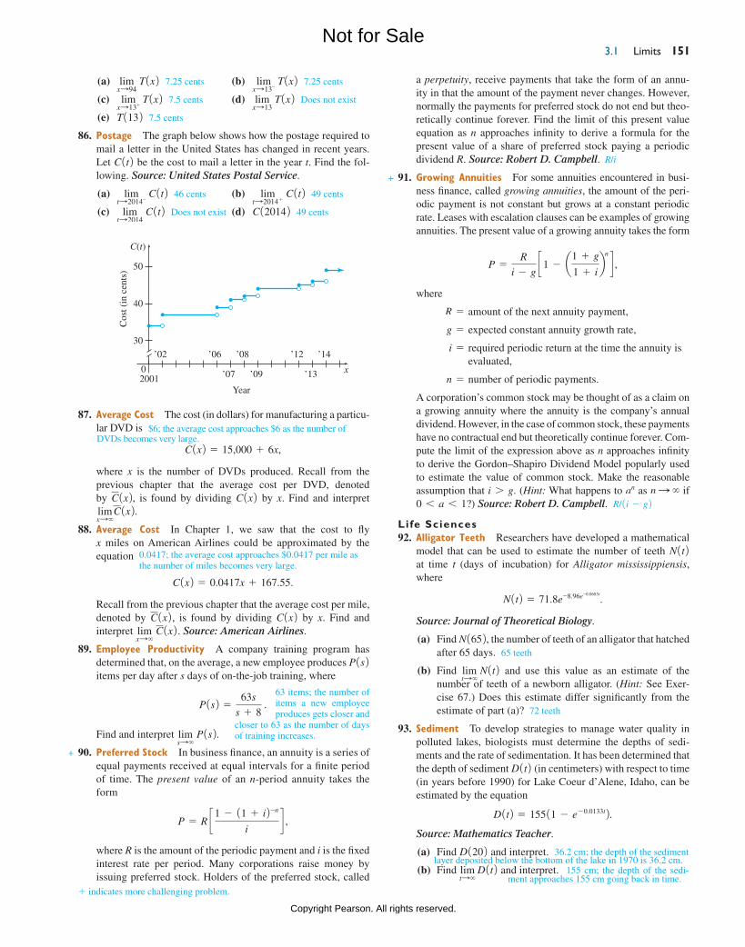
86. Postage The graph below shows how the postage required to mail a letter in the United States has changed in recent years. Let C1t2 be the cost to mail a letter in the year t. Find the fol-lowing. Source: United States Postal Service.
(a) limtS2014-
C1t2 46 cents (b) limtS2014 +
C1t2 49 cents
(c) limtS2014
C1t2 Does not exist (d) C120142 49 cents
+ indicates more challenging problem.
87. Average Cost The cost (in dollars) for manufacturing a particu-lar DVD is
C1x2 = 15,000 + 6x,
where x is the number of DVDs produced. Recall from the previous chapter that the average cost per DVD, denoted by C1x2, is found by dividing C1x2 by x. Find and interpret limxS∞
C1x2. 88. Average Cost In Chapter 1, we saw that the cost to fly
x miles on American Airlines could be approximated by the equation
C1x2 = 0.0417x + 167.55.
Recall from the previous chapter that the average cost per mile, denoted by C1x2, is found by dividing C1x2 by x. Find and interpret lim
xS∞ C1x2. Source: American Airlines.
89. Employee Productivity A company training program has determined that, on the average, a new employee produces P1s2 items per day after s days of on-the-job training, where
P1s2 =63s
s + 8 .
Find and interpret limsS∞
P1s2. 90. Preferred Stock In business finance, an annuity is a series of
equal payments received at equal intervals for a finite period of time. The present value of an n-period annuity takes the form
P = R c 1 - 11 + i2-n
id ,
where R is the amount of the periodic payment and i is the fixed interest rate per period. Many corporations raise money by issuing preferred stock. Holders of the preferred stock, called
+
63 items; the number of items a new employee produces gets closer and
closer to 63 as the number of days of training increases.
$6; the average cost approaches $6 as the number of DVDs becomes very large.
36.2 cm; the depth of the sediment
155 cm; the depth of the sedi-layer deposited below the bottom of the lake in 1970 is 36.2 cm.
ment approaches 155 cm going back in time.
0.0417; the average cost approaches $0.0417 per mile as the number of miles becomes very large.
M03_LIAL8774_11_AIE_C03_133-208.indd 151 03/07/15 12:31 PM
Not for Sale
Copyright Pearson. All rights reserved.
ChAptER 3 the Derivative 152
94. Drug concentration The concentration of a drug in a patient’s bloodstream h hours after it was injected is given by
A1h2 =0.17h
h2 + 2 .
Find and interpret limhS∞
A1h2.Social Sciences 95. legislative Voting Members of a legislature often must vote
repeatedly on the same bill. As time goes on, members may change their votes. Suppose that p0 is the probability that an individual legislator favors an issue before the first roll call vote, and suppose that p is the probability of a change in posi-tion from one vote to the next. Then the probability that the legislator will vote “yes” on the nth roll call is given by
pn =1
2+ ap0 -
1
2b 11 - 2p2n.
For example, the chance of a “yes” on the third roll call vote is
p3 =1
2+ ap0 -
1
2b 11 - 2p23.
Source: Mathematics in the Behavioral and Social Sciences.
Suppose that there is a chance of p0 = 0.7 that Congressman Stephens will favor the budget appropriation bill before the first roll call, but only a probability of p = 0.2 that he will change his mind on the subsequent vote. Find and interpret the following.
(a) p2 0.572 (b) p4 0.526
(c) p8 0.503 (d) limnS∞
pn
YOUR TURN aNSWERS 1. 3 2. 4 3. 5 4. Does not exist.
5. 49 6. -7 7. 1/2 8. 1/3
0; the concentration of the drug in the bloodstream approaches 0 as the number of hours after injection increases.
95. (d) 0.5; the numbers in (a), (b), and (c) give the probability that the legislator will vote yes on the second, fourth, and eighth votes. In (d), as the number of roll calls increases, the probability of a yes vote approaches 0.5 but is never less than 0.5.
continuityHow does the average cost per day of a rental car change with the number of days the car is rented?
APPLY IT
3.2
We will answer this question in Exercise 38.
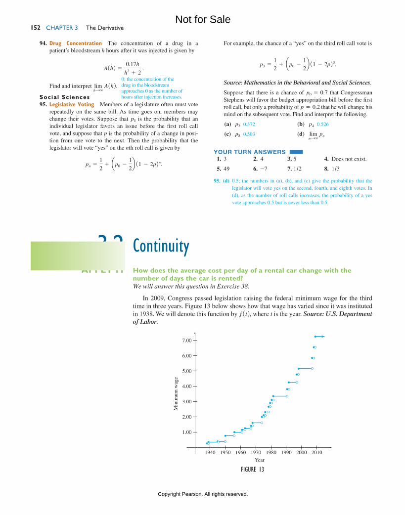
In 2009, Congress passed legislation raising the federal minimum wage for the third time in three years. Figure 13 below shows how that wage has varied since it was instituted in 1938. We will denote this function by ƒ1t2, where t is the year. Source: U.S. Department of Labor.
1940 1950 1960 1970 1980 1990 20102000
1.00
2.00
3.00
4.00
7.00
6.00
5.00
Min
imum
wag
e
Year
Figure 13
M03_LIAL8774_11_AIE_C03_133-208.indd 152 23/06/15 11:31 AM
Not for Sale
Copyright Pearson. All rights reserved.
3.2 Continuity 153
Notice from the graph that limtS1997 -
ƒ1t2 = 4.75 and that limtS1997 +
ƒ1t2 = 5.15, so that
limtS1997
ƒ1t2 does not exist. Notice also that ƒ119972 = 5.15. A point such as this, where a
function has a sudden sharp break, is a point where the function is discontinuous. In this case, the discontinuity is caused by the jump in the minimum wage from $4.75 per hour to $5.15 per hour in 1997.
Intuitively speaking, a function is continuous at a point if you can draw the graph of the function in the vicinity of that point without lifting your pencil from the paper. As we already mentioned, this would not be possible in Figure 13 if it were drawn correctly; there would be a break in the graph at t = 1997, for example. Conversely, a function is discon-tinuous at any x-value where the pencil must be lifted from the paper in order to draw the graph on both sides of the point. A more precise definition is as follows.
continuity at x = cA function ƒ is continuous at x = c if the following three conditions are satisfied:
1. ƒ1c2 is defined,
2. limxSc
ƒ1x2 exists, and
3. limxSc
ƒ1x2 = ƒ1c2.
If ƒ is not continuous at c, it is discontinuous there.
The following example shows how to check a function for continuity at a specific point. We use a three-step test, and if any step of the test fails, the function is not continuous at that point.
Continuity
Determine if each function is continuous at the indicated x-value.
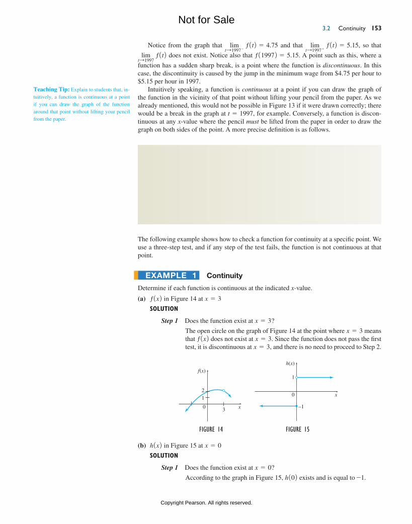
(a) ƒ1x2 in Figure 14 at x = 3
Solution
Step 1 Does the function exist at x = 3?
The open circle on the graph of Figure 14 at the point where x = 3 means that ƒ1x2 does not exist at x = 3. Since the function does not pass the first test, it is discontinuous at x = 3, and there is no need to proceed to Step 2.
ExampLE 1
Teaching Tip: Explain to students that, in-tuitively, a function is continuous at a point if you can draw the graph of the function around that point without lifting your pencil from the paper.
0 3 x
f(x)
2
1
Figure 14
h(x)
0 x
1
–1
Figure 15
(b) h1x2 in Figure 15 at x = 0
Solution
Step 1 Does the function exist at x = 0?
According to the graph in Figure 15, h102 exists and is equal to -1.
M03_LIAL8774_11_AIE_C03_133-208.indd 153 23/06/15 11:31 AM
Not for Sale
Copyright Pearson. All rights reserved.
ChAptER 3 the Derivative 154
Step 2 Does the limit exist at x = 0?
As x approaches 0 from the left, h1x2 is -1. As x approaches 0 from the right, however, h1x2 is 1. In other words,
limxS0-
h1x2 = -1,
while
limxS0 +
h1x2 = 1.
Since no single number is approached by the values of h1x2 as x approaches 0, the limit lim
xS0 h1x2 does not exist. Since the function does not pass the
second test, it is discontinuous at x = 0, and there is no need to proceed to Step 3.
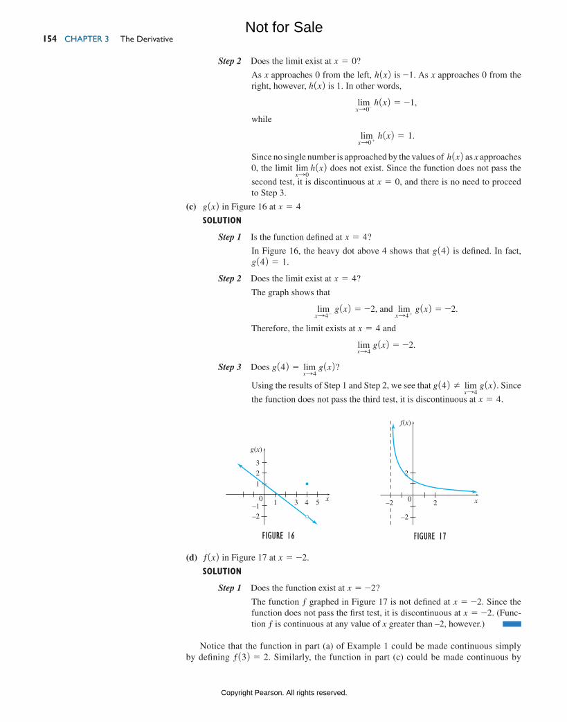
(c) g1x2 in Figure 16 at x = 4
Solution
Step 1 Is the function defined at x = 4?
In Figure 16, the heavy dot above 4 shows that g142 is defined. In fact, g142 = 1.
Step 2 Does the limit exist at x = 4?
The graph shows that
limxS4 -
g1x2 = -2, and limxS4 +
g1x2 = -2.
Therefore, the limit exists at x = 4 and
limxS4
g1x2 = -2.
Step 3 Does g142 = limxS4
g1x2? Using the results of Step 1 and Step 2, we see that g142 Z lim
xS4 g1x2. Since
the function does not pass the third test, it is discontinuous at x = 4.
Figure 17
0 2–2
f(x)
x
2
–2
Figure 16
0 31 4 5
g(x)
x
3
2
1
–1–2
(d) ƒ1x2 in Figure 17 at x = -2.
Solution
Step 1 Does the function exist at x = -2?
The function ƒ graphed in Figure 17 is not defined at x = -2. Since the function does not pass the first test, it is discontinuous at x = -2. (Func-tion ƒ is continuous at any value of x greater than –2, however.)
Notice that the function in part (a) of Example 1 could be made continuous simply by defining ƒ132 = 2. Similarly, the function in part (c) could be made continuous by
M03_LIAL8774_11_AIE_C03_133-208.indd 154 23/06/15 11:31 AM
Not for Sale
Copyright Pearson. All rights reserved.
3.2 Continuity 155
redefining g142 = -2. In such cases, when the function can be made continuous at a specific point simply by defining or redefining it at that point, the function is said to have a removable discontinuity.
A function is said to be continuous on an open interval if it is continuous at every x-value in the interval. Continuity on a closed interval is slightly more complicated because we must decide what to do with the endpoints. We will say that a function ƒ is continuous from the right at x = c if lim
xSc+ ƒ1x2 = ƒ1c2. A function ƒ is continuous from the left at x = c
if limxSc-
ƒ1x2 = ƒ1c2. With these ideas, we can now define continuity on a closed interval.
Figure 18
0
y
x
0.5
1
–0.5
–0.5
–1
–1 10.5
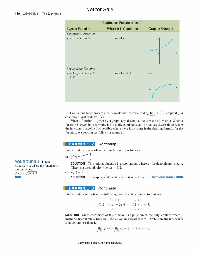
Continuous Functions
Type of Function Where It Is Continuous Graphic Example
Polynomial Function
y = anxn + an-1x
n-1 + g + a1x + a0, where
an, an-1, . . . , a1, a0 are real numbers, not all 0
For all x
Rational Function
y =p1x2q1x2 , where p1x2 and
q1x2 are polynomials, with q1x2 Z 0
For all x where
q1x2 Z 0
Root Function
y = 2ax + b , where a and b are real numbers,
with a Z 0 and ax + b Ú 0
For all x where
ax + b Ú 0
y
x0
y
x0
y
x0
(continued)
continuity on a closed intervalA function is continuous on a closed interval 3a, b4 if
1. it is continuous on the open interval 1a, b2, 2. it is continuous from the right at x = a, and
3. it is continuous from the left at x = b.
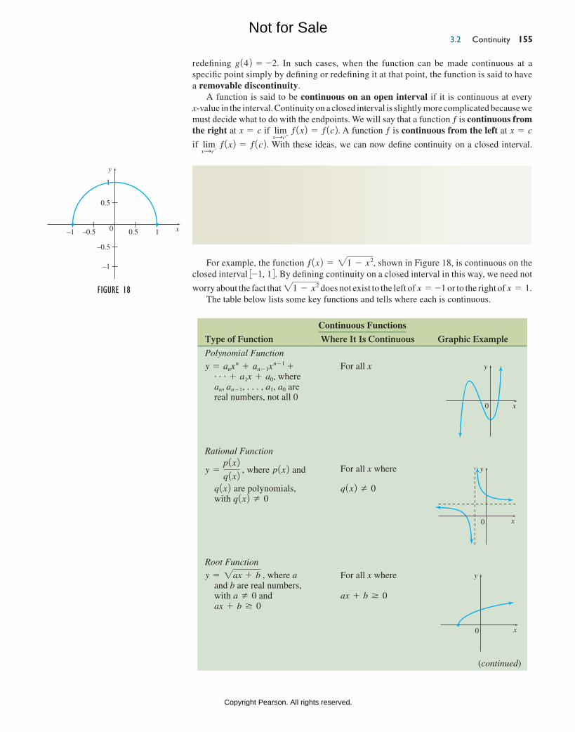
For example, the function ƒ1x2 = 21 - x2, shown in Figure 18, is continuous on the closed interval 3-1, 14. By defining continuity on a closed interval in this way, we need not
worry about the fact that 21 - x2 does not exist to the left of x = -1 or to the right of x = 1.The table below lists some key functions and tells where each is continuous.
M03_LIAL8774_11_AIE_C03_133-208.indd 155 23/06/15 11:31 AM
Not for Sale
Copyright Pearson. All rights reserved.
ChAptER 3 the Derivative 156
Continuous functions are nice to work with because finding limxSc
ƒ1x2 is simple if ƒ is continuous: just evaluate ƒ1c2.
When a function is given by a graph, any discontinuities are clearly visible. When a function is given by a formula, it is usually continuous at all x-values except those where the function is undefined or possibly where there is a change in the defining formula for the function, as shown in the following examples.
Continuous Functions (cont.)
Type of Function Where It Is Continuous Graphic Example
Exponential Function
y = ax where a 7 0 For all x
Logarithmic Function
y = loga x where a 7 0, a Z 1
For all x 7 0
y
x0
y
x0
YOUR TURN 1 Find all values x = a where the function is discontinuous.ƒ1x2 = 25x + 3
Continuity
Find all values x = a where the function is discontinuous.
(a) ƒ1x2 =4x - 3
2x - 7
Solution This rational function is discontinuous wherever the denominator is zero. There is a discontinuity when a = 7/2.
(b) g1x2 = e2x-3
Solution This exponential function is continuous for all x. TRY YOUR TURN 1
ExampLE 2
Continuity
Find all values of x where the following piecewise function is discontinuous.
ƒ1x2 = c x + 1
x2 - 3x + 4
5 - x
if x 6 1
if 1 … x … 3.
if x 7 3
Solution Since each piece of this function is a polynomial, the only x-values where ƒ might be discontinuous here are 1 and 3. We investigate at x = 1 first. From the left, where x-values are less than 1,
limxS1-
ƒ1x2 = limxS1-1x + 12 = 1 + 1 = 2.
ExampLE 3
M03_LIAL8774_11_AIE_C03_133-208.indd 156 23/06/15 11:31 AM
Not for Sale
Copyright Pearson. All rights reserved.
3.2 Continuity 157
From the right, where x-values are greater than 1,
limxS1+
ƒ1x2 = limxS1+1x2 - 3x + 42 = 12 - 3 + 4 = 2.
Furthermore, ƒ112 = 12 - 3 + 4 = 2, so limxS1
ƒ1x2 = ƒ112 = 2. Thus ƒ is continuous at x = 1, since ƒ112 = lim
xS1 ƒ1x2.
Now let us investigate x = 3. From the left,
limxS3-
ƒ1x2 = limxS3-1x2 - 3x + 42 = 32 - 3132 + 4 = 4.
From the right,
limxS3+
ƒ1x2 = limxS3+15 - x2 = 5 - 3 = 2.
Because limxS3-
ƒ1x2 Z limxS3+
ƒ1x2, the limit limxS3
ƒ1x2 does not exist, so ƒ is discontinuous at
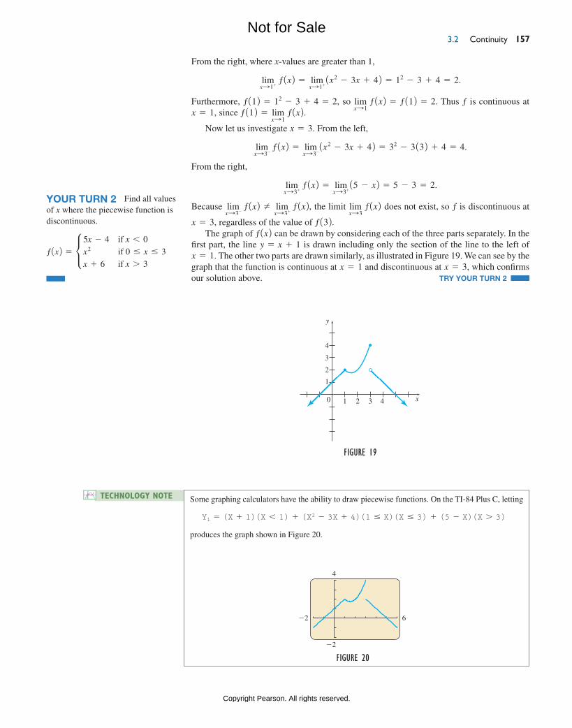
x = 3, regardless of the value of ƒ132.The graph of ƒ1x2 can be drawn by considering each of the three parts separately. In the
first part, the line y = x + 1 is drawn including only the section of the line to the left of x = 1. The other two parts are drawn similarly, as illustrated in Figure 19. We can see by the graph that the function is continuous at x = 1 and discontinuous at x = 3, which confirms our solution above. TRY YOUR TURN 2
YOUR TURN 2 Find all values of x where the piecewise function is discontinuous.
ƒ1x2 = c 5x - 4
x2
x + 6
if x 6 0
if 0 … x … 3
if x 7 3
Figure 19
2
1
3
4
42 310 x
y
technoloGy note Some graphing calculators have the ability to draw piecewise functions. On the TI-84 Plus C, letting
Y1 = (X + 1)(X 6 1) + (X2 - 3X + 4)(1 … X)(X … 3) + (5 - X)(X 7 3)
produces the graph shown in Figure 20.
Figure 20
�2 6
4
�2
M03_LIAL8774_11_AIE_C03_133-208.indd 157 23/06/15 11:31 AM
Not for Sale
Copyright Pearson. All rights reserved.
ChAptER 3 the Derivative 158
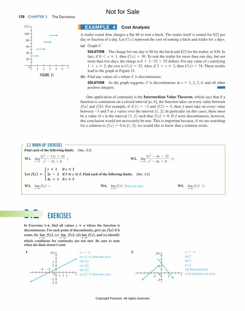
Cost analysis
A trailer rental firm charges a flat $8 to rent a hitch. The trailer itself is rented for $22 per day or fraction of a day. Let C1x2 represent the cost of renting a hitch and trailer for x days.
(a) Graph C.
Solution The charge for one day is $8 for the hitch and $22 for the trailer, or $30. In fact, if 0 6 x … 1, then C1x2 = 30. To rent the trailer for more than one day, but not more than two days, the charge is 8 + 2 # 22 = 52 dollars. For any value of x satisfying 1 6 x … 2, the cost is C1x2 = 52. Also, if 2 6 x … 3, then C1x2 = 74. These results lead to the graph in Figure 21.
(b) Find any values of x where C is discontinuous.
Solution As the graph suggests, C is discontinuous at x = 1, 2, 3, 4, and all other positive integers.
One application of continuity is the Intermediate Value Theorem, which says that if a function is continuous on a closed interval [a, b], the function takes on every value between ƒ1a2 and ƒ1b2. For example, if ƒ112 = -3 and ƒ122 = 5, then ƒ must take on every value between -3 and 5 as x varies over the interval [1, 2]. In particular (in this case), there must be a value of x in the interval 11, 22 such that ƒ1x2 = 0. If ƒ were discontinuous, however, this conclusion would not necessarily be true. This is important because, if we are searching for a solution to ƒ1x2 = 0 in [1, 2], we would like to know that a solution exists.
ExampLE 4
Figure 21
0 21 3 4 5
C(x)
x
100
80
60
40
20
Find each of the following limits. (Sec. 3.1)3.2 warm-up exercises
W1. limxS2
2x2 - 11x + 14
x2 - 5x + 6 3 W2. lim
xS4 3x2 - 4x - 32
x2 - 6x + 8 10
Let ƒ 1x 2 = •x + 1 if x * 32x − 2 if 3 " x " 5.4x + 1 if x + 5
Find each of the following limits. (Sec. 3.1)
W3. limxS3
ƒ1x2 4 W4. limxS5
ƒ1x2 Does not exist W5. limxS6
ƒ1x2 25
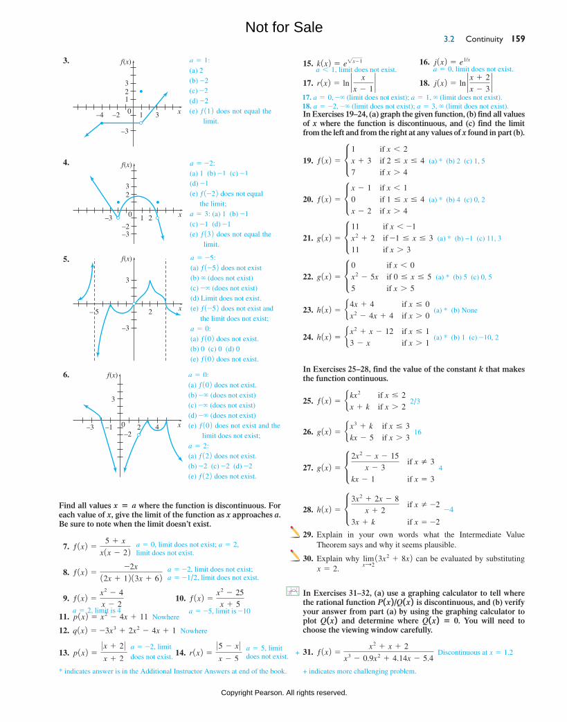
3.2 exercisesIn Exercises 1–6, find all values x = a where the function is discontinuous. For each point of discontinuity, give (a) ƒ 1a 2 if it exists, (b) lim
xSa- ƒ 1x 2 , (c) lim
xSa+ ƒ 1x 2 , (d) lim
xSa ƒ 1x 2 , and (e) identify
which conditions for continuity are not met. Be sure to note when the limit doesn’t exist.
1. f(x)
–3
32
–2210 3 x
–4 –2
2. f(x)
2
–22–2 0 x
a = -1:(a) ƒ1-12 does not exist.(b) 1/2(c) 1/2(d) 1/2(e) ƒ1-12 does not exist.
a = -1:(a) 2(b) 2(c) 4(d) Does not exist.(e) Limit does not exist.
M03_LIAL8774_11_AIE_C03_133-208.indd 158 23/06/15 11:31 AM
Not for Sale
Copyright Pearson. All rights reserved.
3.2 Continuity 159
3. f(x)
123
–3
0 31–2–4 x
4. f(x)
23
–3–2
0 21–3 x
5. f(x)
3
–3
2– 5 x
6. f(x)
3
2–2
4–3 –1 0 x
Find all values x = a where the function is discontinuous. For each value of x, give the limit of the function as x approaches a. Be sure to note when the limit doesn’t exist.
7. ƒ1x2 =5 + x
x1x - 22
8. ƒ1x2 =-2x
12x + 1213x + 62
13. p1x2 =0 x + 2 0x + 2
14. r1x2 =0 5 - x 0x - 5
15. k1x2 = e2x-1 16. j1x2 = e1/x
In Exercises 19–24, (a) graph the given function, (b) find all values of x where the function is discontinuous, and (c) find the limit from the left and from the right at any values of x found in part (b).
19. ƒ1x2 = c 1
x + 3
7
if x 6 2
if 2 … x … 4
if x 7 4
(a) * (b) 2 (c) 1, 5
20. ƒ1x2 = c x - 1
0
x - 2
if x 6 1
if 1 … x … 4
if x 7 4
(a) * (b) 4 (c) 0, 2
21. g1x2 = c 11
x2 + 2
11
if x 6 -1
if -1 … x … 3
if x 7 3
(a) * (b) −1 (c) 11, 3
22. g1x2 = c 0
x2 - 5x
5
if x 6 0
if 0 … x … 5
if x 7 5
(a) * (b) 5 (c) 0, 5
23. h1x2 = b4x + 4
x2 - 4x + 4
if x … 0
if x 7 0 (a) * (b) None
24. h1x2 = b x2 + x - 12
3 - x
if x … 1
if x 7 1 (a) * (b) 1 (c) -10, 2
17. r1x2 = ln ` x
x - 1` 18. j1x2 = ln ` x + 2
x - 3`
a = 1:(a) 2(b) -2(c) -2(d) -2(e) ƒ112 does not equal the
limit.
a = -2:(a) 1 (b) -1 (c) -1(d) -1(e) ƒ1-22 does not equal
the limit;a = 3: (a) 1 (b) -1 (c) -1 (d) -1(e) ƒ132 does not equal the
limit.
a = -5:(a) ƒ1-52 does not exist(b) ∞ (does not exist)(c) -∞ (does not exist)(d) Limit does not exist.(e) ƒ1-52 does not exist and
the limit does not exist;a = 0:(a) ƒ102 does not exist.(b) 0 (c) 0 (d) 0(e) ƒ102 does not exist.
a = 0:(a) ƒ102 does not exist.(b) -∞ (does not exist)(c) -∞ (does not exist)(d) -∞ (does not exist)(e) ƒ102 does not exist and the
limit does not exist;a = 2:(a) ƒ122 does not exist.(b) -2 (c) -2 (d) -2(e) ƒ122 does not exist.
a = 0, limit does not exist; a = 2, limit does not exist.
a = -2, limit does not exist; a = -1/2, limit does not exist.
a = -2, limit does not exist.
a = 5, limit does not exist.
a 6 1, limit does not exist. a = 0, limit does not exist.
9. ƒ1x2 =x2 - 4
x - 2 10. ƒ1x2 =
x2 - 25
x + 5
11. p1x2 = x2 - 4x + 11 Nowhere
12. q1x2 = -3x3 + 2x2 - 4x + 1 Nowhere
a = 2, limit is 4 a = -5, limit is -10
In Exercises 25–28, find the value of the constant k that makes the function continuous.
25. ƒ1x2 = b kx2
x + k
if x … 2
if x 7 2 2/3
26. g1x2 = b x3 + k
kx - 5
if x … 3
if x 7 3 16
27. g1x2 = c 2x2 - x - 15
x - 3
kx - 1
if x Z 3
if x = 3 4
28. h1x2 = c 3x2 + 2x - 8
x + 2
3x + k
if x Z -2
if x = -2
-4
29. Explain in your own words what the Intermediate Value Theorem says and why it seems plausible.
30. Explain why limxS213x2 + 8x2 can be evaluated by substituting
x = 2.
In Exercises 31–32, (a) use a graphing calculator to tell where the rational function P 1x 2 /Q 1x 2 is discontinuous, and (b) verify your answer from part (a) by using the graphing calculator to plot Q 1x 2 and determine where Q 1x 2 = 0. You will need to choose the viewing window carefully.
31. ƒ1x2 =x2 + x + 2
x3 - 0.9x2 + 4.14x - 5.4 Discontinuous at x = 1.2+
* indicates answer is in the Additional Instructor Answers at end of the book. + indicates more challenging problem.
17. a = 0, -∞ (limit does not exist); a = 1, ∞ (limit does not exist).18. a = -2, -∞ (limit does not exist); a = 3, ∞ (limit does not exist).
M03_LIAL8774_11_AIE_C03_133-208.indd 159 23/06/15 11:32 AM
Not for Sale
Copyright Pearson. All rights reserved.
ChAptER 3 the Derivative 160
32. ƒ1x2 =x2 + 3x - 2
x3 - 0.9x2 + 4.14x + 5.4
33. Let g1x2 =x + 4
x2 + 2x - 8. Determine all values of x at which g
is discontinuous, and for each of these values of x, define g in such a manner so as to remove the discontinuity, if possible. Choose one of the following. Source: Society of Actuaries. (a)
(a) g is discontinuous only at -4 and 2. Define g1-42 = -
16 to make g continuous at -4.
g122 cannot be defined to make g continuous at 2.
(b) g is discontinuous only at -4 and 2. Define g1-42 = -
16 to make g continuous at -4.
Define g122 = 6 to make g continuous at 2.
(c) g is discontinuous only at -4 and 2. g1-42 cannot be defined to make g continuous at -4. g(2) cannot be defined to make g continuous at 2.
(d) g is discontinuous only at 2. Define g122 = 6 to make g continuous at 2.
(e) g is discontinuous only at 2. g122 cannot be defined to make g continuous at 2.
34. Tell at what values of x the function ƒ1x2 in Figure 8 from the previous section is discontinuous. Explain why it is discontinu-ous at each of these values.
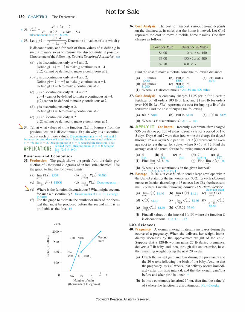
appLicationsBusiness and Economics 35. Production The graph shows the profit from the daily pro-
duction of x thousand kilograms of an industrial chemical. Use the graph to find the following limits.
(a) limxS6
P1x2 $500 (b) limxS10-
P1x2 $1500
(c) limxS10+
P1x2 $1000 (d) limxS10
P1x2 Does not exist
(e) Where is the function discontinuous? What might account for such a discontinuity?
(f ) Use the graph to estimate the number of units of the chem-ical that must be produced before the second shift is as profitable as the first. 15
+
+
36. cost analysis The cost to transport a mobile home depends on the distance, x, in miles that the home is moved. Let C1x2 represent the cost to move a mobile home x miles. One firm charges as follows.
Cost per Mile Distance in Miles
$4.00 0 6 x … 150
$3.00 150 6 x … 400
$2.50 400 6 x
Find the cost to move a mobile home the following distances.
(a) 130 miles (b) 150 miles (c) 210 miles
(d) 400 miles (e) 500 miles
(f ) Where is C discontinuous?
37. cost analysis A company charges $1.25 per lb for a certain fertilizer on all orders 100 lb or less, and $1 per lb for orders over 100 lb. Let F1x2 represent the cost for buying x lb of the fertilizer. Find the cost of buying the following.
(a) 80 lb $100 (b) 150 lb $150 (c) 100 lb
(d) Where is F discontinuous? At x = 100
38. APPLY IT car Rental Recently, a car rental firm charged $36 per day or portion of a day to rent a car for a period of 1 to 5 days. Days 6 and 7 were then free, while the charge for days 8 through 12 was again $36 per day. Let A1t2 represent the aver-age cost to rent the car for t days, where 0 6 t … 12. Find the average cost of a rental for the following number of days.
(a) 4 (b) 5 (c) 6 (d) 7 (e) 8
(f) Find limxS5-
A1t2. 36 (g) Find limxS5+
A1t2. 36
(h) Where is A discontinuous on the given interval?
39. Postage In 2014, it cost $0.98 to send a large envelope within the United States for the first ounce, and $0.21 for each additional ounce, or fraction thereof, up to 13 ounces. Let C1x2 be the cost to mail x ounces. Find the following. Source: U.S. Postal Service.
(a) limxS3-
C1x2 (b) limxS3 +
C1x2 (c) limxS3
C1x2(d) C132 (e) lim
xS8.5-C1x2 (f) lim
xS8.5 +C1x2
(g) limxS8.5
C1x2 (h) C18.52(i) Find all values on the interval 10,132 where the function C
is discontinuous. 1, 2, 3, . . . , 12
Life Sciences 40. Pregnancy A woman’s weight naturally increases during the
course of a pregnancy. When she delivers, her weight imme-diately decreases by the approximate weight of the child. Suppose that a 120-lb woman gains 27 lb during pregnancy, delivers a 7-lb baby, and then, through diet and exercise, loses the remaining weight during the next 20 weeks.
(a) Graph the weight gain and loss during the pregnancy and the 20 weeks following the birth of the baby. Assume that the pregnancy lasts 40 weeks, that delivery occurs immedi-ately after this time interval, and that the weight gain/loss before and after birth is linear. *
(b) Is this a continuous function? If not, then find the value(s) of t where the function is discontinuous. No; 40 weeks
Discontinuous at x = -0.926
P(x)
2000
1500
1000
500
15 206 1050 x
Pro�
t (in
dol
lars
)
Number of units(thousands of kilograms)
(10, 1500)
(10, 1000)
Secondshift
Firstshift
$520 $600 $630
$1200 $1250At 150 and 400 miles
$125
t = 1, 2, 3, 4, 7, 8, 9, 10, 11
$36 $36 $30 $25.71 $27
$1.40 $1.61Does not exist
$1.40 $2.66
$2.66$2.66 $2.66
Discontinuous at x = 10; a change in shifts
because the limit does not exist there. Also, the function is not defined at x = -6 and x = 3. Discontinuous at x = 4 because the function is not
Discontinuous at x = -6, -4, and 3
defined there. Discontinuous at x = 0 because limxS0
ƒ1x2 Z ƒ102.
M03_LIAL8774_11_AIE_C03_133-208.indd 160 23/06/15 11:32 AM
Not for Sale
Copyright Pearson. All rights reserved.
3.3 Rates of Change 161
This question will be answered in Example 4 of this section as we develop a method for finding the rate of change of one variable with respect to a unit change in another variable.
average rate of change One of the main applications of calculus is deter-mining how one variable changes in relation to another. A marketing manager wants to know how profit changes with respect to the amount spent on advertising, while a physician wants to know how a patient’s reaction to a drug changes with respect to the dose.
For example, suppose we take a trip from San Francisco driving south. Every half-hour we note how far we have traveled, with the following results for the first three hours.
Distance Traveled
Time in Hours 0 0.5 1 1.5 2 2.5 3
Distance in Miles 0 30 55 80 104 124 138
If s is the function whose rule is
s1t2 = Distance from San Francisco at time t,
then the table shows, for example, that s102 = 0, s112 = 55, s12.52 = 124, and so on. The distance traveled during, say, the second hour can be calculated by s122 - s112 = 104 - 55 = 49 miles.
Distance equals time multiplied by rate (or speed); so the distance formula is d = rt. Solving for rate gives r = d/t, or
Average speed =Distance
Time .
For example, the average speed over the time interval from t = 0 to t = 3 is
Average speed =s132 - s102
3 - 0=
138 - 0
3= 46,
41. Poultry Farming Researchers at Iowa State University and the University of Arkansas have developed a piecewise function that can be used to estimate the body weight (in grams) of a male broiler during the first 56 days of life according to
W1t2 = e48 + 3.64t + 0.6363t2 + 0.00963t3 if 1 … t … 28,
-1004 + 65.8t if 28 6 t … 56,
where t is the age of the chicken (in days). Source: Poultry Science.
(a) Determine the weight of a male broiler that is 25 days old. About 687 g
(b) Is W1t2 a continuous function? No
(c) Use a graphing calculator to graph W1t2 on 31, 564 by 30, 30004. Comment on the accuracy of the graph. *
(d) Comment on why researchers would use two different types of functions to estimate the weight of a chicken at various ages.
YOUR TURN aNSWERS 1. Discontinuous when a 6 -3/5.
2. Discontinuous at x = 0.
rates of changeHow does the manufacturing cost of a DVD change as the number of DVDs manufactured changes?
APPLY IT
3.3
M03_LIAL8774_11_AIE_C03_133-208.indd 161 23/06/15 11:32 AM
Not for Sale
Copyright Pearson. All rights reserved.
ChAptER 3 the Derivative 162
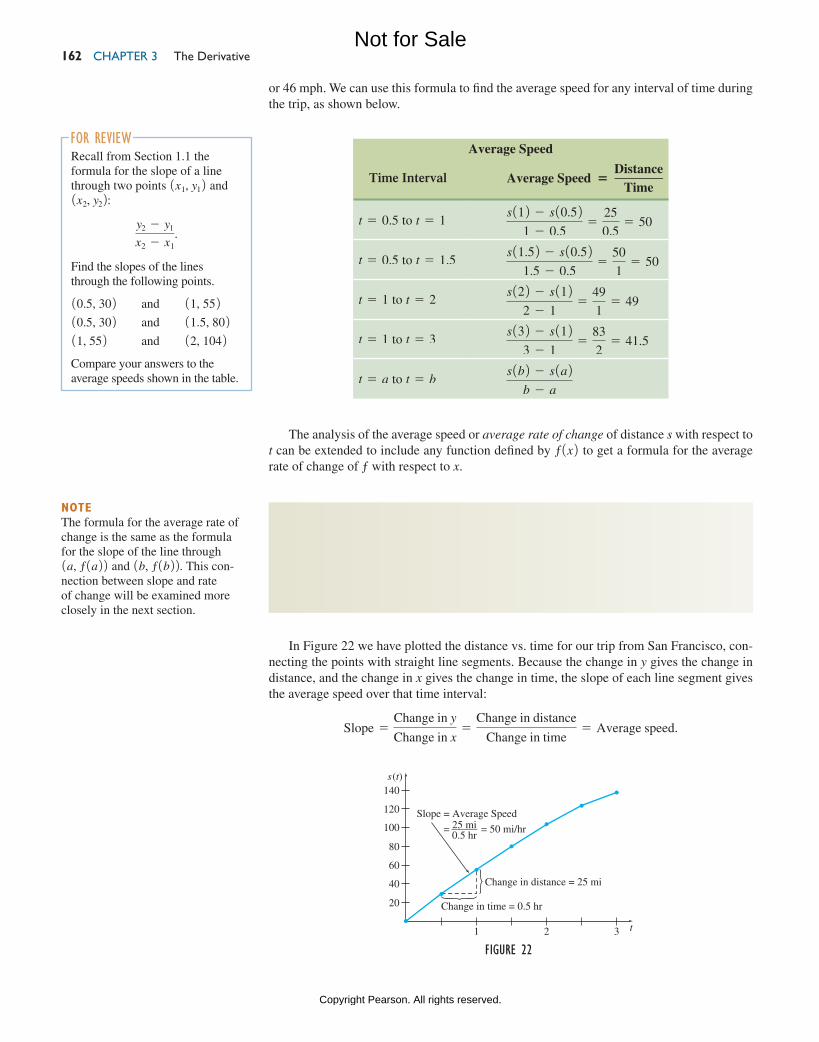
or 46 mph. We can use this formula to find the average speed for any interval of time during the trip, as shown below.
Average Speed
Time Interval Average Speed =Distance
Time
t = 0.5 to t = 1s112 - s10.52
1 - 0.5=
25
0.5= 50
t = 0.5 to t = 1.5s11.52 - s10.52
1.5 - 0.5=
50
1= 50
t = 1 to t = 2s122 - s112
2 - 1=
49
1= 49
t = 1 to t = 3s132 - s112
3 - 1=
83
2= 41.5
t = a to t = bs1b2 - s1a2
b - a
The analysis of the average speed or average rate of change of distance s with respect to t can be extended to include any function defined by ƒ1x2 to get a formula for the average rate of change of ƒ with respect to x.
average rate of changeThe average rate of change of ƒ1x2 with respect to x for a function ƒ as x changes from a to b is
ƒ 1b 2 − ƒ 1a 2b − a
.
In Figure 22 we have plotted the distance vs. time for our trip from San Francisco, con-necting the points with straight line segments. Because the change in y gives the change in distance, and the change in x gives the change in time, the slope of each line segment gives the average speed over that time interval:
Slope =Change in y
Change in x=
Change in distance
Change in time= Average speed.
noteThe formula for the average rate of change is the same as the formula for the slope of the line through 1a, ƒ1a22 and 1b, ƒ1b22. This con-nection between slope and rate of change will be examined more closely in the next section.
For reviewRecall from Section 1.1 the formula for the slope of a line through two points 1x1, y12 and 1x2, y22:
y2 - y1
x2 - x1.
Find the slopes of the lines through the following points.
10.5, 302 and 11, 552 10.5, 302 and 11.5, 802 11, 552 and 12, 1042Compare your answers to the average speeds shown in the table.
Figure 221 2 3
s(t)
20
40
60
80
100
120
140
Change in time = 0.5 hr
Change in distance = 25 mi
Slope = Average Speed25 mi0.5 hr
= = 50 mi/hr
t
M03_LIAL8774_11_AIE_C03_133-208.indd 162 23/06/15 11:32 AM
Not for Sale
Copyright Pearson. All rights reserved.
3.3 Rates of Change 163
minority population
The United States population is becoming more diverse. Based on the U.S. Census popula-tion projections for 2000 to 2050, the projected Hispanic population (in millions) can be modeled by the exponential function
H1t2 = 37.79111.0212t,
where t = 0 corresponds to 2000 and 0 … t … 50. Use H to estimate the average rate of change in the Hispanic population from 2000 to 2010. Source: U.S. Census Bureau.
Solution On the interval from t = 0 120002 to t = 10 120102, the average rate of change was
H1102 - H102
10 - 0=
37.79111.021210 - 37.79111.02120
10
≈46.521 - 37.791
10=
8.73
10
= 0.873,
or 0.873 million. Based on this model, it is estimated that the Hispanic population in the United States increased, on average, at a rate of about 873,000 people per year between 2000 and 2010. TRY YOUR TURN 1
Education Spending
Figure 23 below shows the total amount appropriated annually (in billions of dollars) for the U.S. Department of Education in recent years. Find the average rate of change per year in Department of Education appropriation from 2009 to 2013. Source: U.S. Department of Education.
ExampLE 1
ExampLE 2
YOUR TURN 1 The projected U.S. Asian population (in millions) for this same time period is A1t2 = 11.1411.0232t. Use A to estimate the average rate of change from 2000 to 2010.
Figure 23 2008 2009
63.5264.14
68.35 68.11
65.70
2010 2011 2012 2014201363
64
65
66
67
68
69
Am
ount
(in
bill
ions
of
dolla
rs)
Solution Let A1t2 be the total amount appropriated for the Department of Education (in billions of dollars) in the year t. Then the average rate of change from 2009 to 2013 was
A120132 - A1200922013 - 2009
=65.70 - 63.52
4=
2.18
4= 0.545.
On average, the amount appropriated went up by 0.545 billion dollars, or $545 million, per year during these years. TRY YOUR TURN 2
instantaneous rate of change Suppose a car is stopped at a traffic light. When the light turns green, the car begins to move along a straight road. Assume that the distance traveled by the car is given by the function
s1t2 = 3t2, for 0 … t … 15,
YOUR TURN 2 In Example 2, find the average rate of change per year in the amount appropriated for the Department of Education from 2011 to 2013.
M03_LIAL8774_11_AIE_C03_133-208.indd 163 23/06/15 11:32 AM
Not for Sale
Copyright Pearson. All rights reserved.
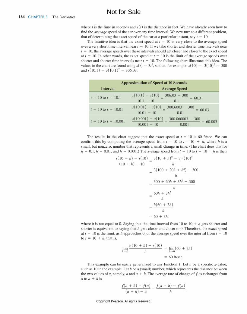
ChAptER 3 the Derivative 164
where t is the time in seconds and s1t2 is the distance in feet. We have already seen how to find the average speed of the car over any time interval. We now turn to a different problem, that of determining the exact speed of the car at a particular instant, say t = 10.
The intuitive idea is that the exact speed at t = 10 is very close to the average speed over a very short time interval near t = 10. If we take shorter and shorter time intervals near t = 10, the average speeds over these intervals should get closer and closer to the exact speed at t = 10. In other words, the exact speed at t = 10 is the limit of the average speeds over shorter and shorter time intervals near t = 10. The following chart illustrates this idea. The values in the chart are found using s1t2 = 3t2, so that, for example, s1102 = 311022 = 300 and s110.12 = 3110.122 = 306.03.
Approximation of Speed at 10 Seconds
Interval Average Speed
t = 10 to t = 10.1s110.12 - s1102
10.1 - 10=
306.03 - 300
0.1= 60.3
t = 10 to t = 10.01s110.012 - s1102
10.01 - 10=
300.6003 - 300
0.01= 60.03
t = 10 to t = 10.001s110.0012 - s1102
10.001 - 10=
300.060003 - 300
0.001= 60.003
The results in the chart suggest that the exact speed at t = 10 is 60 ft/sec. We can confirm this by computing the average speed from t = 10 to t = 10 + h, where h is a small, but nonzero, number that represents a small change in time. (The chart does this for h = 0.1, h = 0.01, and h = 0.001.) The average speed from t = 10 to t = 10 + h is then
s110 + h2 - s1102110 + h2 - 10
=3110 + h22 - 3 # 11022
h
=31100 + 20h + h22 - 300
h
=300 + 60h + 3h2 - 300
h
=60h + 3h2
h
=h160 + 3h2
h
= 60 + 3h,
where h is not equal to 0. Saying that the time interval from 10 to 10 + h gets shorter and shorter is equivalent to saying that h gets closer and closer to 0. Therefore, the exact speed at t = 10 is the limit, as h approaches 0, of the average speed over the interval from t = 10 to t = 10 + h; that is,
limhS0
s 110 + h2 - s1102
h = lim
hS0160 + 3h2
= 60 ft/sec.
This example can be easily generalized to any function ƒ. Let a be a specific x-value, such as 10 in the example. Let h be a (small) number, which represents the distance between the two values of x, namely, a and a + h. The average rate of change of ƒ as x changes from a to a + h is
ƒ1a + h2 - ƒ1a21a + h2 - a
=ƒ1a + h2 - ƒ1a2
h ,
M03_LIAL8774_11_AIE_C03_133-208.indd 164 23/06/15 11:32 AM
Not for Sale
Copyright Pearson. All rights reserved.
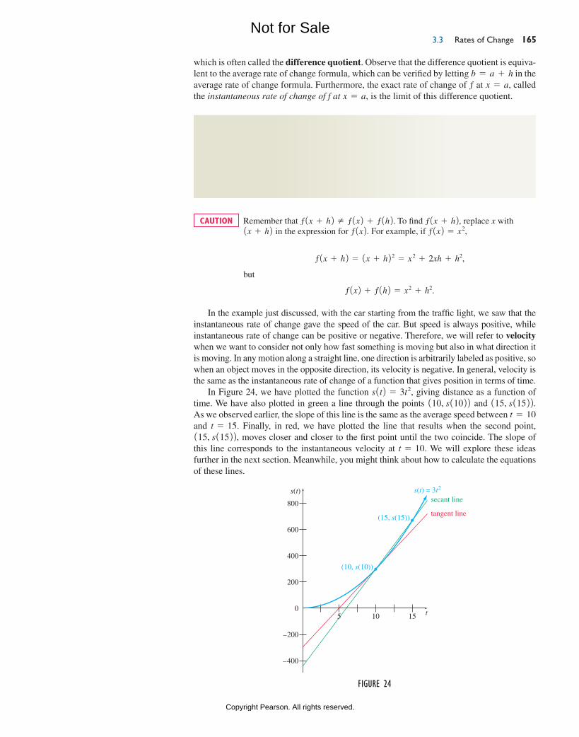
3.3 Rates of Change 165
which is often called the difference quotient. Observe that the difference quotient is equiva-lent to the average rate of change formula, which can be verified by letting b = a + h in the average rate of change formula. Furthermore, the exact rate of change of ƒ at x = a, called the instantaneous rate of change of f at x = a, is the limit of this difference quotient.
instantaneous rate of changeThe instantaneous rate of change for a function ƒ when x = a is
limhS0
f 1a + h 2 − f 1a 2
h ,
provided this limit exists.
Remember that ƒ1x + h2 Z ƒ1x2 + ƒ1h2. To find ƒ1x + h2, replace x with 1x + h2 in the expression for ƒ1x2. For example, if ƒ1x2 = x2,
ƒ1x + h2 = 1x + h22 = x2 + 2xh + h2,
but
ƒ1x2 + ƒ1h2 = x2 + h2.
In the example just discussed, with the car starting from the traffic light, we saw that the instantaneous rate of change gave the speed of the car. But speed is always positive, while instantaneous rate of change can be positive or negative. Therefore, we will refer to velocity when we want to consider not only how fast something is moving but also in what direction it is moving. In any motion along a straight line, one direction is arbitrarily labeled as positive, so when an object moves in the opposite direction, its velocity is negative. In general, velocity is the same as the instantaneous rate of change of a function that gives position in terms of time.
In Figure 24, we have plotted the function s1t2 = 3t2, giving distance as a function of time. We have also plotted in green a line through the points 110, s11022 and 115, s11522. As we observed earlier, the slope of this line is the same as the average speed between t = 10 and t = 15. Finally, in red, we have plotted the line that results when the second point, 115, s11522, moves closer and closer to the first point until the two coincide. The slope of this line corresponds to the instantaneous velocity at t = 10. We will explore these ideas further in the next section. Meanwhile, you might think about how to calculate the equations of these lines.
caution
Figure 24
800
600
400
200
–200
0
–400
5 10 15
s(t)
t
(10, s(10))
(15, s(15))
s(t) = 3t2
secant line
tangent line
M03_LIAL8774_11_AIE_C03_133-208.indd 165 23/06/15 11:32 AM
Not for Sale
Copyright Pearson. All rights reserved.
ChAptER 3 the Derivative 166
An alternate, but equivalent, approach is to let a + h = b in the definition for instan-taneous rate of change, so that h = b - a. This makes the instantaneous rate of change formula look more like the average rate of change formula.
Method 1 Standard From
Method 2 alternate From
instantaneous rate of change (alternate Form)The instantaneous rate of change for a function ƒ when x = a can be written as
limbSa
ƒ 1b 2 − ƒ 1a 2
b − a ,
provided this limit exists.
Velocity
The distance in feet of an object from a starting point is given by s1t2 = 2t2 - 5t + 40, where t is time in seconds.
(a) Find the average velocity of the object from 2 seconds to 4 seconds.
Solution The average velocity is
s142 - s1224 - 2
=52 - 38
2=
14
2= 7,
or 7 ft per second.
(b) Find the instantaneous velocity at 4 seconds.
Solution
For t = 4, the instantaneous velocity is
limhS0
s14 + h2 - s142
h
ft per second. We first calculate s14 + h2 and s142, that is,
s14 + h2 = 214 + h22 - 514 + h2 + 40
= 2116 + 8h + h22 - 20 - 5h + 40
= 32 + 16h + 2h2 - 20 - 5h + 40
= 2h2 + 11h + 52,
and
s142 = 21422 - 5142 + 40 = 52.
Therefore, the instantaneous velocity at t = 4 is
limhS0
12h2 + 11h + 522 - 52
h= lim
hS0 2h2 + 11h
h= lim
hS0
h12h + 112h
= limhS012h + 112 = 11,
or 11 ft per second.
For t = 4, the instantaneous velocity is
limbS4
s1b2 - s142
b - 4
ft per second. We first calculate s1b2 and s142, that is,
s1b2 = 2b2 - 5b + 40
ExampLE 3
M03_LIAL8774_11_AIE_C03_133-208.indd 166 23/06/15 11:32 AM
Not for Sale
Copyright Pearson. All rights reserved.
3.3 Rates of Change 167
and
s142 = 21422 - 5142 + 40 = 52.
The instantaneous rate of change is then
limbS4
2b2 - 5b + 40 - 52
b - 4= lim
bS4 2b2 - 5b - 12
b - 4 Simplify the numerator.
= limbS4
12b + 321b - 42b - 4
Factor the numerator.
= limbS4
12b + 32 Cancel the b − 4.
= 11, Calculate the limit.
or 11 ft per second. TRY YOUR TURN 3
manufacturing
A company determines that the cost in dollars to manufacture x cases of the DVD “Math-ematicians Caught in Embarrassing Moments” is given by
C1x2 = 100 + 15x - x2 10 … x … 72.(a) Find the average change, per case, in the total cost if the number of cases manufactured
changes from 1 to 5 cases.
Solution Use the formula for average rate of change. The average rate of change of cost is
C152 - C1125 - 1
=150 - 114
4= 9.
Thus, the total cost, on average, increases by $9 for each additional case when produc-tion increased from 1 to 5 cases.
(b) Find the additional cost when production is increased from 1 to 2 cases.
Solution The additional cost can be found by calculating the cost to produce 2 cases, and subtracting the cost to produce 1 case; that is,
C122 - C112 = 126 - 114 = 12.
The additional cost to produce the second case is $12.
(c) Find the instantaneous rate of change of cost with respect to the number of cases pro-duced when just one case is produced.
Solution The instantaneous rate of change for x = 1 is given by
limhS0
C11 + h2 - C112
h
= limhS0
3100 + 1511 + h2 - 11 + h224 - 3100 + 15112 - 124
h
= limhS0
100 + 15 + 15h - 1 - 2h - h2 - 114
h
= limhS0
13h - h2
h Combine terms.
= limhS0
h113 - h2
h Factor.
= limhS0113 - h2 Divide by h.
= 13. Calculate the limit.
ExampLE 4
APPLY IT
YOUR TURN 3 For the func-tion in Example 3, find the instanta-neous velocity at 2 seconds.
M03_LIAL8774_11_AIE_C03_133-208.indd 167 23/06/15 11:32 AM
Not for Sale
Copyright Pearson. All rights reserved.
ChAptER 3 the Derivative 168
When 1 case is manufactured, the cost is increasing at the rate of $13 per case. Notice that this is close to the value calculated in part (b).
As we mentioned in Chapter 1, economists sometimes define the marginal cost as the cost of producing one additional item and sometimes as the instantaneous rate of change of the cost function. These definitions are considered to be essentially equivalent. If a company (or an econ-omy) produces millions of items, it makes little difference whether we let h = 1 or take the limit as h goes to 0, because 1 is very close to 0 when production is in the millions. The advantage of taking the instantaneous rate of change point of view is that it allows all the power of calculus to be used, including the Fundamental Theorem of Calculus, which is discussed later in this book.
Throughout this textbook, we define the marginal cost to be the instantaneous rate of change of the cost function. It can then be interpreted as the approximate cost of producing one additional item. For simplicity, we will make this interpretation even when production numbers are fairly small.
manufacturing
For the cost function in the previous example, find the instantaneous rate of change of cost when 5 cases are made.
Solution The instantaneous rate of change for x = 5 is given by
limhS0
C15 + h2 - C152
h
= limhS0
3100 + 1515 + h2 - 15 + h224 - 3100 + 15152 - 524
h
= limhS0
100 + 75 + 15h - 25 - 10h - h2 - 150
h
= limhS0
5h - h2
h Combine terms.
= limhS0
h15 - h2
h Factor.
= limhS015 - h2 Divide by h.
= 5. Calculate the limit.
When 5 cases are manufactured, the cost is increasing at the rate of $5 per case; that is, the marginal cost when x = 5 is $5. Notice that as the number of items produced goes up, the marginal cost goes down, as might be expected. TRY YOUR TURN 4
minority population
Estimate the instantaneous rate of change in 2010 in the Hispanic population of the United States.
Solution We saw in Example 1 that the U.S. Hispanic population is approximately given by H1t2 = 37.79111.0212t, where t = 0 corresponds to 2000. Unlike the previous example, in which the function was a polynomial, the function in this example is an exponential, mak-ing it harder to compute the limit directly using the formula for instantaneous rate of change at t = 10 (the year 2010):
limhS0
37.79111.021210+h - 37.79111.021210
h.
Instead, we will approximate the instantaneous rate of change by using smaller and smaller values of h. See the table on the next page. The limit seems to be approaching 0.96682 (million). Thus, the instantaneous rate of change in the U.S. Hispanic population was about 966,820 people per year in 2010. TRY YOUR TURN 5
ExampLE 5
ExampLE 6
Teaching Tip: We will define marginal cost (or revenue or profit) as the instanta-neous rate of change of the cost (or revenue or profit) function. We will interpret it as the approximate cost (or revenue or profit) of one additional item.
YOUR TURN 4 If the cost function is given by C1x2 = x2 - 2x + 12, find the instantaneous rate of change of cost when x = 4.
YOUR TURN 5 Estimate the instantaneous rate of change in 2010 in the Asian population of the United States. An estimate of the U.S. Asian population is given by A1t2 = 11.1411.0232t, where t = 0 corresponds to 2000.
M03_LIAL8774_11_AIE_C03_133-208.indd 168 23/06/15 11:32 AM
Not for Sale
Copyright Pearson. All rights reserved.
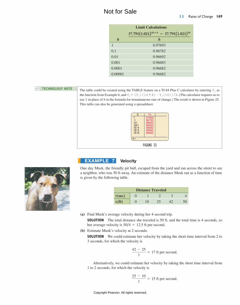
3.3 Rates of Change 169
Velocity
One day Musk, the friendly pit bull, escaped from the yard and ran across the street to see a neighbor, who was 50 ft away. An estimate of the distance Musk ran as a function of time is given by the following table.
Distance Traveled
t (sec) 0 1 2 3 4
s (ft) 0 10 25 42 50
(a) Find Musk’s average velocity during her 4-second trip.
Solution The total distance she traveled is 50 ft, and the total time is 4 seconds, so her average velocity is 50/4 = 12.5 ft per second.
(b) Estimate Musk’s velocity at 2 seconds.
Solution We could estimate her velocity by taking the short time interval from 2 to 3 seconds, for which the velocity is
42 - 25
1= 17 ft per second.
Alternatively, we could estimate her velocity by taking the short time interval from 1 to 2 seconds, for which the velocity is
25 - 10
1= 15 ft per second.
ExamplE 7
Limit Calculations
h
37.791 11.021 2 10+h − 37.791 11.021 2 10
h
1 0.97693
0.1 0.96782
0.01 0.96692
0.001 0.96683
0.0001 0.96682
0.00001 0.96682
technology note The table could be created using the TABLE feature on a TI-84 Plus C calculator by entering Y1 as the function from Example 6, and Y2 = (Y1)(10 + X) – Y1(10))/X. (The calculator requires us to use X in place of h in the formula for instantaneous rate of change.) The result is shown in Figure 25. This table can also be generated using a spreadsheet.
Figure 25
1.1.01.0011E-41E-51E-6
.97693
.96782
.96692
.96683
.96682
.96682
.96682
Y2.97693.96782.96692.96683.96682.96682.96682
X�
X Y2
M03_LIAL8774_11_AIE_C03_133-208.indd 169 03/07/15 12:31 PM
Not for Sale
Copyright Pearson. All rights reserved.
ChAptER 3 the Derivative 170
A better estimate is found by averaging these two values to get
17 + 15
2= 16 ft per second.
Another way to get this same answer is to take the time interval from 1 to 3 seconds, for which the velocity is
42 - 10
2= 16 ft per second.
This answer is reasonable if we assume Musk’s velocity changes at a fairly steady rate and does not increase or decrease drastically from one second to the next. It is impossible to calculate Musk’s exact velocity without knowing her position at times arbitrarily close to 2 seconds, or without a formula for her position as a function of time, or without a radar gun or speedometer on her. (In any case, she was very happy when she reached the neighbor.)
Suppose the position of an object moving in a straight line is given by s 1 t 2 = 5t2 − 2t − 7. Find the instantaneous velocity at each time. 23. Explain the difference between the average rate of change of y
as x changes from a to b, and the instantaneous rate of change of y at x = a.
21. ƒ1x2 = x ln x at x = 2 22. ƒ1x2 = x ln x at x = 3
Use the formula for instantaneous rate of change, approximating the limit by using smaller and smaller values of h, to find the instantaneous rate of change for each function at the given value.
11. t = 2 18 12. t = 3 28
19. ƒ1x2 = xx at x = 2 6.773 20. ƒ1x2 = xx at x = 3 56.66 9. t = 6 17 10. t = 1 7
1.121
3.3 exercisesFind the average rate of change for each function over the given interval.
1. y = x2 + 2x between x = 1 and x = 3 6
2. y = -4x2 - 6 between x = 2 and x = 6 -32
3. y = -3x3 + 2x2 - 4x + 1 between x = -2 and x = 1
4. y = 2x3 - 4x2 + 6x between x = -1 and x = 4 20
5. y = 2x between x = 1 and x = 4 1/3
6. y = 23x - 2 between x = 1 and x = 2 1
7. y = ex between x = -2 and x = 0 0.4323
8. y = ln x between x = 2 and x = 4 0.3466
Suppose the position of an object moving in a straight line is given by s 1t 2 = t2 + 5t + 2. Find the instantaneous velocity at each time.
Find the instantaneous rate of change for each function at the given value.
15. ƒ1x2 = x2 + 2x at x = 0 2
16. s1t2 = -4t2 - 6 at t = 2 -16
17. g1t2 = 1 - t2 at t = -1 2
18. F1x2 = x2 + 2 at x = 0 0
Suppose the position of an object moving in a straight line is given by s 1t 2 = t3 + 2t + 9. Find the instantaneous velocity at each time.
13. t = 1 5 14. t = 4 50
-15
2.449
For the function ƒ 1x 2 = 2x2 + 3x + 4, find and simplify each of the following. (Sec. 2.1)
W1. ƒ15 + h2 2h2 + 23h + 69 W2. ƒ12 + h2 - ƒ122
h 2h + 11
For the function ƒ 1x 2 = 2x + 1
, find and simplify each of the
following. (Sec. 2.1)
W3. ƒ13 + h2 2/14 + h2 W4. ƒ14 + h2 - ƒ142
h -2/3515 + h24
3.3 warm-up exercises
M03_LIAL8774_11_AIE_C03_133-208.indd 170 23/06/15 11:32 AM
Not for Sale
Copyright Pearson. All rights reserved.
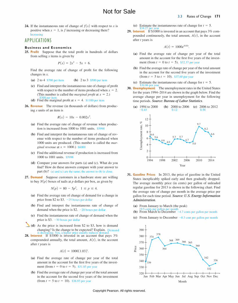
3.3 Rates of Change 171
24. If the instantaneous rate of change of ƒ1x2 with respect to x is positive when x = 1, is ƒ increasing or decreasing there?
appLicationsBusiness and Economics 25. Profit Suppose that the total profit in hundreds of dollars
from selling x items is given by
P1x2 = 2x2 - 5x + 6.
Find the average rate of change of profit for the following changes in x.
(a) 2 to 4 $700 per item (b) 2 to 3 $500 per item
(c) Find and interpret the instantaneous rate of change of profit with respect to the number of items produced when x = 2. (This number is called the marginal profit at x = 2.)
(d) Find the marginal profit at x = 4. $1100 per item
26. Revenue The revenue (in thousands of dollars) from produc-ing x units of an item is
R1x2 = 10x - 0.002x2.
(a) Find the average rate of change of revenue when produc-tion is increased from 1000 to 1001 units. $5998
(b) Find and interpret the instantaneous rate of change of rev-enue with respect to the number of items produced when 1000 units are produced. (This number is called the mar-ginal revenue at x = 1000.) $6000
(c) Find the additional revenue if production is increased from 1000 to 1001 units. $5998
(d) Compare your answers for parts (a) and (c). What do you find? How do these answers compare with your answer to part (b)? (a) and (c) are the same; the answer to (b) is close.
27. Demand Suppose customers in a hardware store are willing to buy N1p2 boxes of nails at p dollars per box, as given by
N1p2 = 80 - 5p2, 1 … p … 4.
(a) Find the average rate of change of demand for a change in price from $2 to $3. -25 boxes per dollar
(b) Find and interpret the instantaneous rate of change of demand when the price is $2. -20 boxes per dollar
(c) Find the instantaneous rate of change of demand when the price is $3. -30 boxes per dollar
(d) As the price is increased from $2 to $3, how is demand changing? Is the change to be expected? Explain.
28. interest If $1000 is invested in an account that pays 3% compounded annually, the total amount, A1t2, in the account after t years is
A1t2 = 100011.032t.(a) Find the average rate of change per year of the total
amount in the account for the first five years of the invest-ment (from t = 0 to t = 5). $31.85 per year
(b) Find the average rate of change per year of the total amount in the account for the second five years of the investment (from t = 5 to t = 10). $36.93 per year
(c) Estimate the instantaneous rate of change for t = 5.
29. interest If $1000 is invested in an account that pays 3% com-pounded continuously, the total amount, A1t2, in the account after t years is
A1t2 = 1000e0.03t.
(a) Find the average rate of change per year of the total amount in the account for the first five years of the invest-ment (from t = 0 to t = 5). $32.37 per year
(b) Find the average rate of change per year of the total amount in the account for the second five years of the investment (from t = 5 to t = 10). $37.60 per year
(c) Estimate the instantaneous rate of change for t = 5.
30. unemployment The unemployment rates in the United States for the years 1994–2014 are shown in the graph below. Find the average change per year in unemployment for the following time periods. Source: Bureau of Labor Statistics.
(a) 1994 to 2000 (b) 2000 to 2006 (c) 2006 to 2012
$300 per item
Demand
$34.27 per year
$34.86 per year
1994
6.65.6
4.64.0
5.7 5.74.7
5.0
9.7
8.2
6.6
1998 2002 2006
Year
2010 20140
2
4
6
8
10
12
Une
mpl
oym
ent r
ate,
%
31. Gasoline Prices In 2013, the price of gasoline in the United States inexplicably spiked early and then gradually dropped. The average monthly price (in cents) per gallon of unleaded regular gasoline for 2013 is shown in the following chart. Find the average rate of change per month in the average price per gallon for each time period. Source: U.S. Energy Information Administration.
(a) From January to March (the peak)
(b) From March to December -4.7 cents per gallon per month
(c) From January to December -0.3 cent per gallon per month
Jan Feb Apr Jun
Month
Aug DecMar May Jul Sep Oct Nov320
330
340
360
350
370
380
390
Pric
e
339
374378
364
366 365360
342336
332
368 369
-0.43 0.12 0.58
19.5 cents per gallon per month
Increasing
is decreasing. Yes, a higher price usually reduces demand.
M03_LIAL8774_11_AIE_C03_133-208.indd 171 23/06/15 11:32 AM
Not for Sale
Copyright Pearson. All rights reserved.
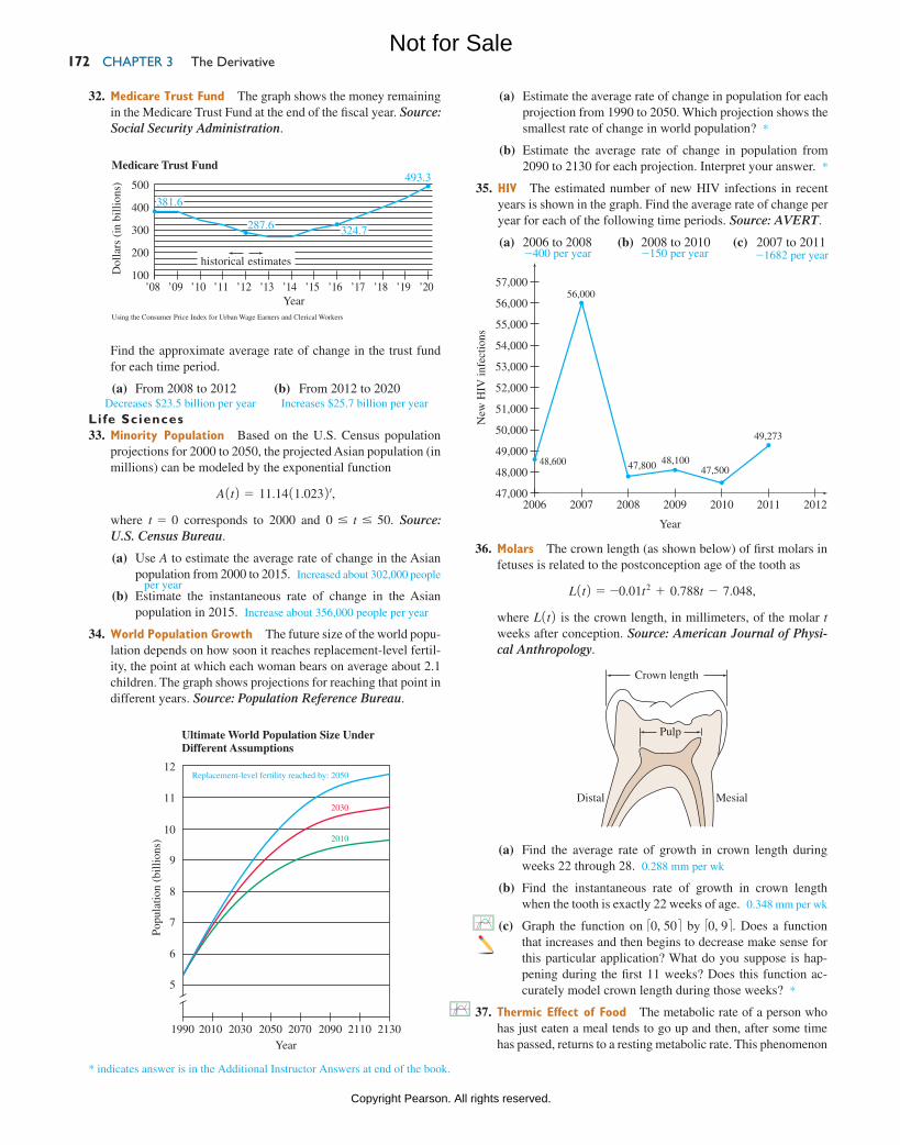
ChAptER 3 the Derivative 172
32. Medicare trust Fund The graph shows the money remaining in the Medicare Trust Fund at the end of the fiscal year. Source: Social Security Administration.
(a) Estimate the average rate of change in population for each projection from 1990 to 2050. Which projection shows the smallest rate of change in world population? *
(b) Estimate the average rate of change in population from 2090 to 2130 for each projection. Interpret your answer. *
35. hiV The estimated number of new HIV infections in recent years is shown in the graph. Find the average rate of change per year for each of the following time periods. Source: AVERT.
(a) 2006 to 2008 (b) 2008 to 2010 (c) 2007 to 2011
400
500
300
100
200
’08 ’09 ’10 ’11 ’12 ’20’19’18’17’16’15’14’13Year
Medicare Trust Fund
Dol
lars
(in
bill
ions
)
Using the Consumer Price Index for Urban Wage Earners and Clerical Workers
historical estimates
381.6
287.6 324.7
493.3
Find the approximate average rate of change in the trust fund for each time period.
(a) From 2008 to 2012 (b) From 2012 to 2020
Life Sciences 33. Minority Population Based on the U.S. Census population
projections for 2000 to 2050, the projected Asian population (in millions) can be modeled by the exponential function
A1t2 = 11.1411.0232t, where t = 0 corresponds to 2000 and 0 … t … 50. Source:
U.S. Census Bureau.
(a) Use A to estimate the average rate of change in the Asian population from 2000 to 2015. Increased about 302,000 people
per year(b) Estimate the instantaneous rate of change in the Asian
population in 2015. Increase about 356,000 people per year
34. World Population Growth The future size of the world popu-lation depends on how soon it reaches replacement-level fertil-ity, the point at which each woman bears on average about 2.1 children. The graph shows projections for reaching that point in different years. Source: Population Reference Bureau.
Decreases $23.5 billion per year Increases $25.7 billion per year
12
11
9
8
7
6
10
5
2050 2070 2090 2110 2130203020101990
Popu
latio
n (b
illio
ns)
Year
Ultimate World Population Size UnderDifferent Assumptions
Replacement-level fertility reached by: 2050
2030
2010
2006
48,60047,500
49,273
47,800 48,100
56,000
Year
2007 2008 2009 2010 2011 201247,000
48,000
49,000
50,000
52,000
51,000
53,000
54,000
55,000
56,000
57,000
New
HIV
infe
ctio
ns
36. Molars The crown length (as shown below) of first molars in fetuses is related to the postconception age of the tooth as
L1t2 = -0.01t2 + 0.788t - 7.048,
where L1t2 is the crown length, in millimeters, of the molar t weeks after conception. Source: American Journal of Physi-cal Anthropology.
-400 per year -150 per year -1682 per year
* indicates answer is in the Additional Instructor Answers at end of the book.
Crown length
Distal Mesial
Pulp
(a) Find the average rate of growth in crown length during weeks 22 through 28. 0.288 mm per wk
(b) Find the instantaneous rate of growth in crown length when the tooth is exactly 22 weeks of age. 0.348 mm per wk
(c) Graph the function on 30, 504 by 30, 94. Does a function that increases and then begins to decrease make sense for this particular application? What do you suppose is hap-pening during the first 11 weeks? Does this function ac-curately model crown length during those weeks? *
37. thermic effect of Food The metabolic rate of a person who has just eaten a meal tends to go up and then, after some time has passed, returns to a resting metabolic rate. This phenomenon
M03_LIAL8774_11_AIE_C03_133-208.indd 172 23/06/15 11:32 AM
Not for Sale
Copyright Pearson. All rights reserved.
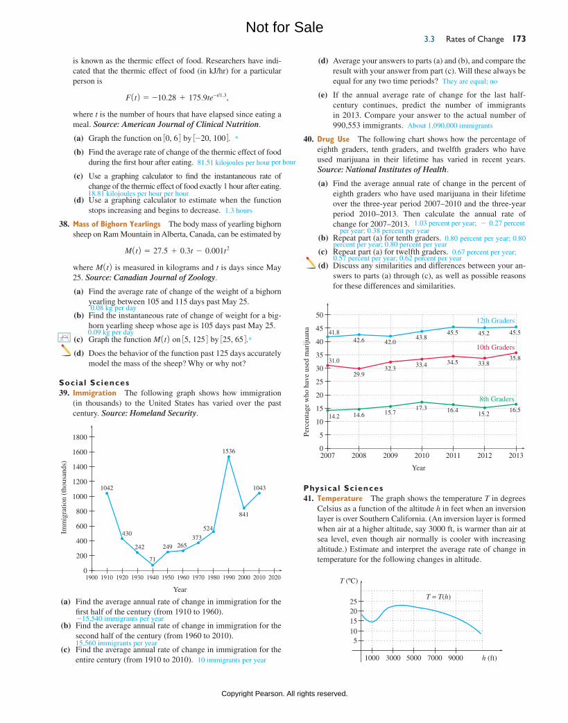
3.3 Rates of Change 173
is known as the thermic effect of food. Researchers have indi-cated that the thermic effect of food (in kJ/hr) for a particular person is
F1t2 = -10.28 + 175.9te-t/1.3,
where t is the number of hours that have elapsed since eating a meal. Source: American Journal of Clinical Nutrition.
(a) Graph the function on 30, 64 by 3-20, 1004. *
(b) Find the average rate of change of the thermic effect of food during the first hour after eating.
(c) Use a graphing calculator to find the instantaneous rate of change of the thermic effect of food exactly 1 hour after eating.
(d) Use a graphing calculator to estimate when the function stops increasing and begins to decrease. 1.3 hours
38. Mass of Bighorn yearlings The body mass of yearling bighorn sheep on Ram Mountain in Alberta, Canada, can be estimated by
M1t2 = 27.5 + 0.3t - 0.001t2
where M1t2 is measured in kilograms and t is days since May 25. Source: Canadian Journal of Zoology.
(a) Find the average rate of change of the weight of a bighorn yearling between 105 and 115 days past May 25.
(b) Find the instantaneous rate of change of weight for a big-horn yearling sheep whose age is 105 days past May 25.
(c) Graph the function M1t2 on 35, 1254 by 325, 654.*(d) Does the behavior of the function past 125 days accurately
model the mass of the sheep? Why or why not?
Social Sciences 39. immigration The following graph shows how immigration
(in thousands) to the United States has varied over the past century. Source: Homeland Security.
(d) Average your answers to parts (a) and (b), and compare the result with your answer from part (c). Will these always be equal for any two time periods? They are equal; no
(e) If the annual average rate of change for the last half-century continues, predict the number of immigrants in 2013. Compare your answer to the actual number of 990,553 immigrants. About 1,090,000 immigrants
40. Drug use The following chart shows how the percentage of eighth graders, tenth graders, and twelfth graders who have used marijuana in their lifetime has varied in recent years. Source: National Institutes of Health.
(a) Find the average annual rate of change in the percent of eighth graders who have used marijuana in their lifetime over the three-year period 2007–2010 and the three-year period 2010–2013. Then calculate the annual rate of change for 2007–2013.
(b) Repeat part (a) for tenth graders.
(c) Repeat part (a) for twelfth graders.
(d) Discuss any similarities and differences between your an-swers to parts (a) through (c), as well as possible reasons for these differences and similarities.
0.08 kg per day
0.09 kg per day
1900 1910
1042
430
242 249 265373
524
1536
841
1043
71
1930 1950
Year
1970 20101920 1940 1960 1980 1990 2000 20200
200
400
800
600
1000
1200
1400
1600
1800
Imm
igra
tion
(tho
usan
ds)
(a) Find the average annual rate of change in immigration for the first half of the century (from 1910 to 1960).
(b) Find the average annual rate of change in immigration for the second half of the century (from 1960 to 2010).
(c) Find the average annual rate of change in immigration for the entire century (from 1910 to 2010). 10 immigrants per year
-15,540 immigrants per year
15,560 immigrants per year
1.03 percent per year; - 0.27 percent per year; 0.38 percent per year
0.80 percent per year; 0.80 percent per year; 0.80 percent per year
0.67 percent per year; 0.57 percent per year; 0.62 percent per year
2007
14.2 14.6 15.7 16.417.315.2
16.5
31.0
29.932.3
34.533.4 33.835.8
41.842.6 42.0
45.543.8
45.2 45.5
Year
12th Graders
10th Graders
8th Graders
2008 2009 2010 2011 2012 20130
5
10
15
25
20
30
35
40
45
50Pe
rcen
tage
who
hav
e us
ed m
ariju
ana
T (ºC)
252015105
7000500030001000 9000 h (ft)
T = T(h)
Physical Sciences 41. temperature The graph shows the temperature T in degrees
Celsius as a function of the altitude h in feet when an inversion layer is over Southern California. (An inversion layer is formed when air at a higher altitude, say 3000 ft, is warmer than air at sea level, even though air normally is cooler with increasing altitude.) Estimate and interpret the average rate of change in temperature for the following changes in altitude.
18.81 kilojoules per hour per hour
81.51 kilojoules per hour per hour
M03_LIAL8774_11_AIE_C03_133-208.indd 173 23/06/15 11:32 AM
Not for Sale
Copyright Pearson. All rights reserved.
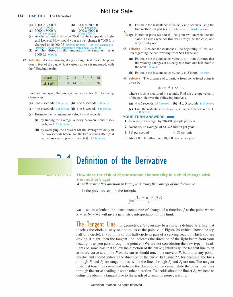
ChAptER 3 the Derivative 174
(c) 3000 to 9000 ft (d) 1000 to 9000 ft
(e) At what altitude at or below 7000 ft is the temperature high-est? Lowest? How would your answer change if 7000 ft is changed to 10,000 ft?
(f) At what altitude is the temperature the same as it is at 1000 ft? 9000 ft
42. Velocity A car is moving along a straight test track. The posi-tion in feet of the car, s1t2, at various times t is measured, with the following results.
t (sec) 0 2 4 6 8 10
s 1 t 2 (ft) 0 10 14 20 30 36
Find and interpret the average velocities for the following changes in t.
(a) 0 to 2 seconds 5 ft per sec (b) 2 to 4 seconds 2 ft per sec
(c) 4 to 6 seconds 3 ft per sec (d) 6 to 8 seconds 5 ft per sec
(e) Estimate the instantaneous velocity at 4 seconds
(i) by finding the average velocity between 2 and 6 sec-onds, and 2.5 ft per sec;
(ii) by averaging the answers for the average velocity in the two seconds before and the two seconds after (that is, the answers to parts (b) and (c)). 2.5 ft per sec
(f) Estimate the instantaneous velocity at 6 seconds using the two methods in part (e). (i) 4 ft per sec; (ii) 4 ft per sec
(g) Notice in parts (e) and (f) that your two answers are the same. Discuss whether this will always be the case, and why or why not.
43. Velocity Consider the example at the beginning of this sec-tion regarding the car traveling from San Francisco.
(a) Estimate the instantaneous velocity at 1 hour. Assume that the velocity changes at a steady rate from one half-hour to the next. 50 mph
(b) Estimate the instantaneous velocity at 2 hours. 44 mph
44. Velocity The distance of a particle from some fixed point is given by
s1t2 = t2 + 5t + 2,
where t is time measured in seconds. Find the average velocity of the particle over the following intervals.
(a) 4 to 6 seconds 15 ft per sec (b) 4 to 5 seconds 14 ft per sec
(c) Find the instantaneous velocity of the particle when t = 4.
YOUR TURN aNSWERS 1. Increase, on average, by 284,000 people per year
2. Decrease, on average, of $1.325 billion per year
3. 3 ft per second 4. $6 per unit
5. About 0.318 million, or 318,000 people per year
-4/3° per 1000 ft 0° per 1000 ft
3000 ft; 1000 ft; if 7000 ft is changed to 10,000 ft, the lowest temperature would be at 10,000 ft.
13 ft per sec
Definition of the DerivativeHow does the risk of chromosomal abnormality in a child change with the mother’s age?
APPLY IT
3.4We will answer this question in Example 3, using the concept of the derivative.
In the previous section, the formula
limhS0
ƒ1a + h2 - ƒ1a2
h
was used to calculate the instantaneous rate of change of a function ƒ at the point where x = a. Now we will give a geometric interpretation of this limit.
the tangent Line In geometry, a tangent line to a circle is defined as a line that touches the circle at only one point, as at the point P in Figure 26 (which shows the top half of a circle). If you think of this half-circle as part of a curving road on which you are driving at night, then the tangent line indicates the direction of the light beam from your headlights as you pass through the point P. (We are not considering the new type of head-lights on some cars that follow the direction of the curve.) Intuitively, the tangent line to an arbitrary curve at a point P on the curve should touch the curve at P, but not at any points nearby, and should indicate the direction of the curve. In Figure 27, for example, the lines through P1 and P3 are tangent lines, while the lines through P2 and P5 are not. The tangent lines just touch the curve and indicate the direction of the curve, while the other lines pass through the curve heading in some other direction. To decide about the line at P4, we need to define the idea of a tangent line to the graph of a function more carefully.
(a) 1000 to 3000 ft (b) 1000 to 5000 ft4° per 1000 ft 1.75° per 1000 ft
M03_LIAL8774_11_AIE_C03_133-208.indd 174 23/06/15 11:32 AM
Not for Sale
Copyright Pearson. All rights reserved.
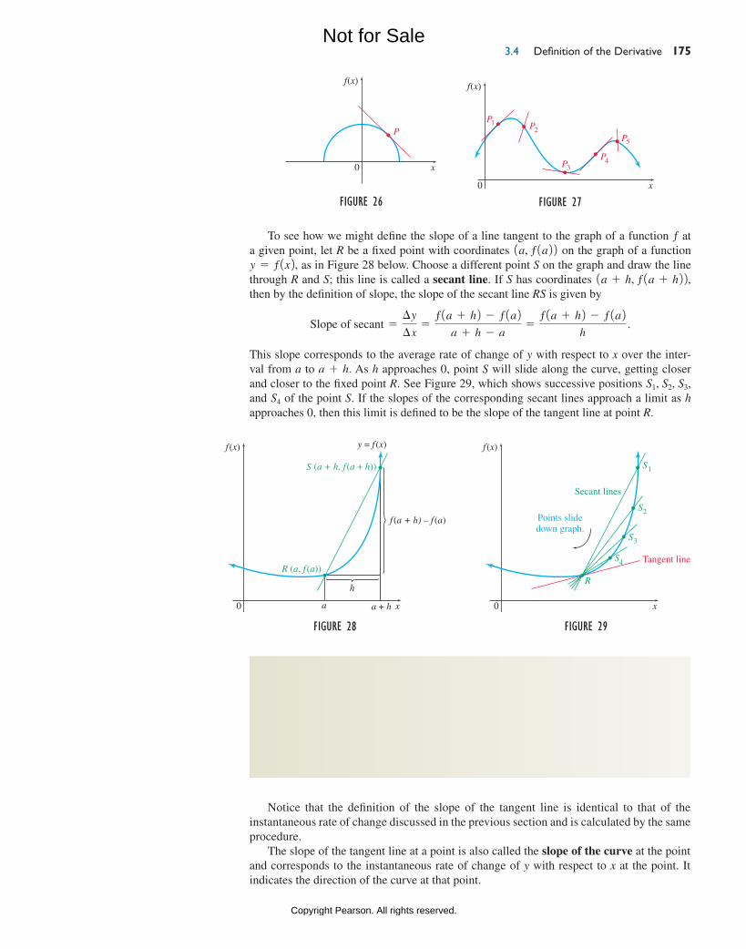
3.4 Definition of the Derivative 175
Figure 26
f(x)
0 x
P
Figure 27
f(x)
0 x
PP
PP
P2
1
34
5
To see how we might define the slope of a line tangent to the graph of a function ƒ at a given point, let R be a fixed point with coordinates 1a, ƒ1a22 on the graph of a function y = ƒ1x2, as in Figure 28 below. Choose a different point S on the graph and draw the line through R and S; this line is called a secant line. If S has coordinates 1a + h, ƒ1a + h22, then by the definition of slope, the slope of the secant line RS is given by
Slope of secant =∆y
∆x=
ƒ1a + h2 - ƒ1a2a + h - a
=ƒ1a + h2 - ƒ1a2
h .
This slope corresponds to the average rate of change of y with respect to x over the inter-val from a to a + h. As h approaches 0, point S will slide along the curve, getting closer and closer to the fixed point R. See Figure 29, which shows successive positions S1, S2, S3, and S4 of the point S. If the slopes of the corresponding secant lines approach a limit as h approaches 0, then this limit is defined to be the slope of the tangent line at point R.
Figure 28
R (a, f (a))
S
a + h
h
f (a + h) – f (a)
(a + h, f (a + h))
a
y = f (x)f (x)
0 x
Figure 29
f (x)
0 x
S
S
S
S
R
Points slidedown graph.
Secant lines
Tangent line
2
1
3
4
slope of the tangent LineThe tangent line of the graph of y = ƒ1x2 at the point 1a, ƒ1a22 is the line through this point having slope
limhS0
ƒ 1a + h 2 − ƒ 1a 2
h ,
provided this limit exists. If this limit does not exist, then there is no tangent at the point.
Notice that the definition of the slope of the tangent line is identical to that of the instantaneous rate of change discussed in the previous section and is calculated by the same procedure.
The slope of the tangent line at a point is also called the slope of the curve at the point and corresponds to the instantaneous rate of change of y with respect to x at the point. It indicates the direction of the curve at that point.
M03_LIAL8774_11_AIE_C03_133-208.indd 175 23/06/15 11:32 AM
Not for Sale
Copyright Pearson. All rights reserved.
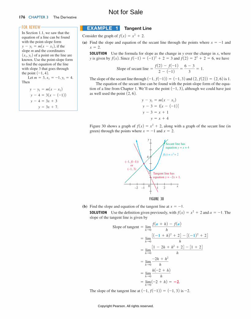
ChAptER 3 the Derivative 176
Tangent Line
Consider the graph of ƒ1x2 = x2 + 2.
(a) Find the slope and equation of the secant line through the points where x = -1 and x = 2.
Solution Use the formula for slope as the change in y over the change in x, where y is given by ƒ1x2. Since ƒ1-12 = 1-122 + 2 = 3 and ƒ122 = 22 + 2 = 6, we have
Slope of secant line =ƒ122 - ƒ1-12
2 - 1-12 =6 - 3
3= 1.
The slope of the secant line through 1-1, ƒ1-122 = 1-1, 32 and 12, ƒ1222 = 12, 62 is 1.The equation of the secant line can be found with the point-slope form of the equa-
tion of a line from Chapter 1. We’ll use the point 1-1, 32, although we could have just as well used the point 12, 62.
y - y1 = m1x - x12 y - 3 = 13x - 1-124y - 3 = x + 1
y = x + 4
Figure 30 shows a graph of ƒ1x2 = x2 + 2, along with a graph of the secant line (in green) through the points where x = -1 and x = 2.
ExampLE 1
Figure 30
0 1–1 2–2
y
x
4
2
f(x) = x + 22
Tangent line hasequation y = –2x + 1.
Secant line hasequation y = x + 4
(–1, f(–1))or
(–1, 3)
(b) Find the slope and equation of the tangent line at x = -1.
Solution Use the definition given previously, with ƒ1x2 = x2 + 2 and a = -1. The slope of the tangent line is given by
Slope of tangent = limhS0
ƒ1a + h2 - ƒ1a2
h
= limhS0
31−1 + h22 + 24 - 31−122 + 24
h
= limhS0
31 - 2h + h2 + 24 - 31 + 24
h
= limhS0
-2h + h2
h
= limhS0
h1-2 + h2
h
= limhS01-2 + h2 = −2.
The slope of the tangent line at 1-1, ƒ1-122 = 1-1, 32 is -2.
For reviewIn Section 1.1, we saw that the equation of a line can be found with the point-slope formy - y1 = m1x - x12, if the slope m and the coordinates 1x1, y12 of a point on the line are known. Use the point-slope form to find the equation of the line with slope 3 that goes through the point 1-1, 42.
Let m = 3, x1 = -1, y1 = 4. Then
y - y1 = m1x - x12 y - 4 = 31x - 1-122 y - 4 = 3x + 3
y = 3x + 7.
M03_LIAL8774_11_AIE_C03_133-208.indd 176 23/06/15 11:32 AM
Not for Sale
Copyright Pearson. All rights reserved.
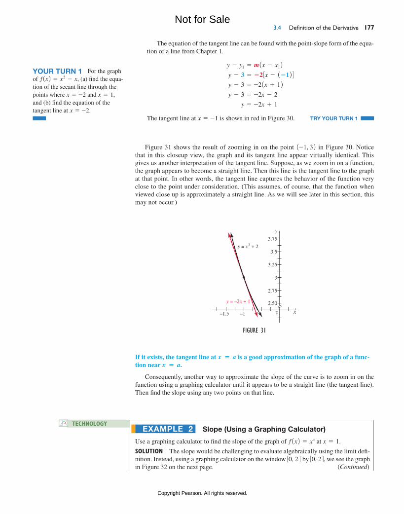
3.4 Definition of the Derivative 177
The equation of the tangent line can be found with the point-slope form of the equa-tion of a line from Chapter 1.
y - y1 = m1x - x12 y - 3 = −2 3x - 1−124 y - 3 = -21x + 12 y - 3 = -2x - 2
y = -2x + 1
The tangent line at x = -1 is shown in red in Figure 30. TRY YOUR TURN 1
YOUR TURN 1 For the graph of ƒ1x2 = x2 - x, (a) find the equa-tion of the secant line through the points where x = -2 and x = 1, and (b) find the equation of the tangent line at x = -2.
Figure 31
2.50
2.75
3
3.75
3.5
3.25
–1–1.5 0 x
y
y = x2 + 2
y = –2x + 1
Slope (Using a Graphing Calculator)
Use a graphing calculator to find the slope of the graph of ƒ1x2 = xx at x = 1.
Solution The slope would be challenging to evaluate algebraically using the limit defi-nition. Instead, using a graphing calculator on the window 30, 24 by 30, 24, we see the graph in Figure 32 on the next page.
ExampLE 2technoloGy
(Continued)
Figure 31 shows the result of zooming in on the point 1-1, 32 in Figure 30. Notice that in this closeup view, the graph and its tangent line appear virtually identical. This gives us another interpretation of the tangent line. Suppose, as we zoom in on a function, the graph appears to become a straight line. Then this line is the tangent line to the graph at that point. In other words, the tangent line captures the behavior of the function very close to the point under consideration. (This assumes, of course, that the function when viewed close up is approximately a straight line. As we will see later in this section, this may not occur.)
If it exists, the tangent line at x = a is a good approximation of the graph of a func-tion near x = a.
Consequently, another way to approximate the slope of the curve is to zoom in on the function using a graphing calculator until it appears to be a straight line (the tangent line). Then find the slope using any two points on that line.
M03_LIAL8774_11_AIE_C03_133-208.indd 177 23/06/15 11:32 AM
Not for Sale
Copyright Pearson. All rights reserved.
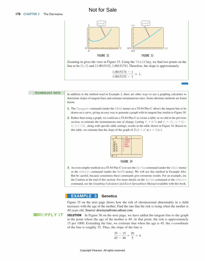
Chapter 3 the Derivative 178
Zooming in gives the view in Figure 33. Using the TRACE key, we find two points on the line to be 11, 12 and 11.0015152, 1.00151742. Therefore, the slope is approximately
1.0015174 - 1
1.0015152 - 1≈ 1.
0 2
2
0
y � x x
Figure 32
0.9 1.1
1.1
0.9
y � x x
Figure 33
Technology noTe In addition to the method used in Example 2, there are other ways to use a graphing calculator to determine slopes of tangent lines and estimate instantaneous rates. Some alternate methods are listed below.
1. The Tangent command (under the DRAW menu) on a TI-84 Plus C allows the tangent line to be drawn on a curve, giving an easy way to generate a graph with its tangent line similar to Figure 30.
2. Rather than using a graph, we could use a TI-84 Plus C to create a table, as we did in the previous section, to estimate the instantaneous rate of change. Letting Y1 = X^X and Y2 = (Y1(1 + X)— Y1(1))/X, along with specific table settings, results in the table shown in Figure 34. Based on this table, we estimate that the slope of the graph of ƒ1x2 = xx at x = 1 is 1.
Figure 34
1.01.0011E-41E-51E-6
1.10531.01011.0011.000111
Y21.10531.01011.0011.000111
X�.1
X Y2
3. An even simpler method on a TI-84 Plus C is to use the dy/dx command (under the CALC menu) or the nDeriv command (under the MATH menu). We will use this method in Example 4(b). But be careful, because sometimes these commands give erroneous results. For an example, see the Caution at the end of this section. For more details on the dy/dx command or the nDeriv command, see the Graphing Calculator and Excel Spreadsheet Manual available with this book.
Genetics
Figure 35 on the next page shows how the risk of chromosomal abnormality in a child increases with the age of the mother. Find the rate that the risk is rising when the mother is 40 years old. Source: downsyndrome.about.com.
SoluTion In Figure 36 on the next page, we have added the tangent line to the graph at the point where the age of the mother is 40. At that point, the risk is approximately 15 per 1000. Extending the line, we estimate that when the age is 45, the y-coordinate of the line is roughly 35. Thus, the slope of the line is
35 - 15
45 - 40=
20
5= 4.
ExamplE 3
APPLY IT
M03_LIAL8774_11_AIE_C03_133-208.indd 178 03/07/15 12:31 PM
Not for Sale
Copyright Pearson. All rights reserved.
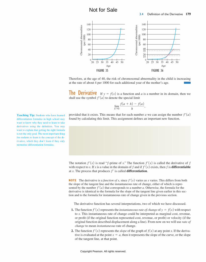
3.4 Definition of the Derivative 179
DerivativeThe derivative of the function ƒ at x is defined as
ƒ′ 1x 2 = limhS0
ƒ 1x + h 2 − ƒ 1x 2
h ,
provided this limit exists.
Chr
omos
omal
abn
orm
aliti
es(p
er 1
000)
Age
100
120
140
60
80
20
40
302520 35 40 45 500
Figure 35
Chr
omos
omal
abn
orm
aliti
es(p
er 1
000)
Age
100
120
140
60
80
2015
4035
302520 35 40 45 500
Figure 36
Teaching Tip: Students who have learned differentiation formulas in high school may want to know why they need to learn to take derivatives using the definition. You may want to explain that getting the right formula is not the only goal. The most important thing for students to learn is the concept of the de-rivative, which they don’t learn if they only memorize differentiation formulas.
note The derivative is a function of x, since ƒ′1x2 varies as x varies. This differs from both the slope of the tangent line and the instantaneous rate of change, either of which is repre-sented by the number ƒ′1a2 that corresponds to a number a. Otherwise, the formula for the derivative is identical to the formula for the slope of the tangent line given earlier in this sec-tion and to the formula for instantaneous rate of change given in the previous section.
The derivative function has several interpretations, two of which we have discussed.
1. The function ƒ′1x2 represents the instantaneous rate of change of y = ƒ1x2 with respect to x. This instantaneous rate of change could be interpreted as marginal cost, revenue, or profit (if the original function represented cost, revenue, or profit) or velocity (if the original function described displacement along a line). From now on we will use rate of change to mean instantaneous rate of change.
2. The function ƒ′1x2 represents the slope of the graph of ƒ1x2 at any point x. If the deriva-tive is evaluated at the point x = a, then it represents the slope of the curve, or the slope of the tangent line, at that point.
The notation ƒ′1x2 is read “ƒ-prime of x.” The function ƒ′1x2 is called the derivative of ƒ with respect to x. If x is a value in the domain of ƒ and if ƒ′1x2 exists, then ƒ is differentiable at x. The process that produces ƒ′ is called differentiation.
Therefore, at the age of 40, the risk of chromosomal abnormality in the child is increasing at the rate of about 4 per 1000 for each additional year of the mother’s age.
the Derivative If y = ƒ1x2 is a function and a is a number in its domain, then we shall use the symbol ƒ′1a2 to denote the special limit
limhS0
ƒ1a + h2 - ƒ1a2
h ,
provided that it exists. This means that for each number a we can assign the number ƒ′1a2 found by calculating this limit. This assignment defines an important new function.
M03_LIAL8774_11_AIE_C03_133-208.indd 179 23/06/15 11:32 AM
Not for Sale
Copyright Pearson. All rights reserved.
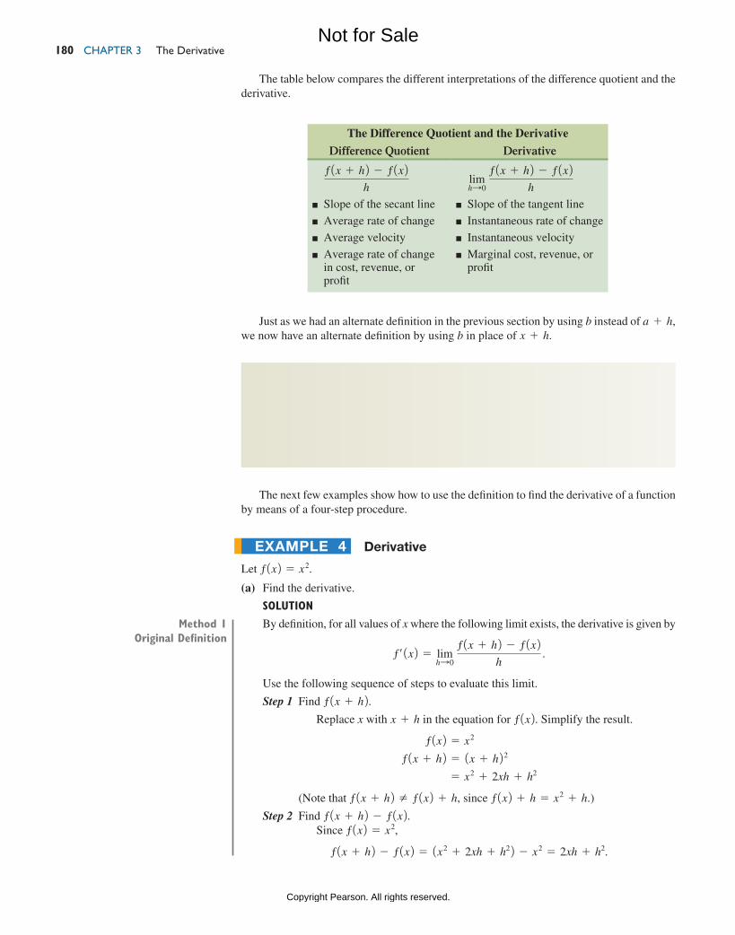
ChAptER 3 the Derivative 180
Just as we had an alternate definition in the previous section by using b instead of a + h, we now have an alternate definition by using b in place of x + h.
Derivative (alternate Form)The derivative of function ƒ at x can be written as
ƒ′ 1x 2 = limbSx
ƒ 1b 2 − ƒ 1x 2
b − x ,
provided this limit exists.
The next few examples show how to use the definition to find the derivative of a function by means of a four-step procedure.
Derivative
Let ƒ1x2 = x2.
(a) Find the derivative.
Solution
By definition, for all values of x where the following limit exists, the derivative is given by
ƒ′1x2 = limhS0
ƒ1x + h2 - ƒ1x2
h .
Use the following sequence of steps to evaluate this limit.
Step 1 Find ƒ1x + h2.Replace x with x + h in the equation for ƒ1x2. Simplify the result.
ƒ1x2 = x2
ƒ1x + h2 = 1x + h22
= x2 + 2xh + h2
(Note that ƒ1x + h2 Z ƒ1x2 + h, since ƒ1x2 + h = x2 + h.)
Step 2 Find ƒ1x + h2 - ƒ1x2.Since ƒ1x2 = x2,
ƒ1x + h2 - ƒ1x2 = 1x2 + 2xh + h22 - x2 = 2xh + h2.
ExampLE 4
The Difference Quotient and the Derivative
Difference Quotient Derivative
ƒ1x + h2 - ƒ1x2h
limhS0
ƒ1x + h2 - ƒ1x2
h
■ Slope of the secant line
■ Average rate of change
■ Average velocity
■ Average rate of change in cost, revenue, or profit
■ Slope of the tangent line
■ Instantaneous rate of change
■ Instantaneous velocity
■ Marginal cost, revenue, or profit
Method 1 original Definition
The table below compares the different interpretations of the difference quotient and the derivative.
M03_LIAL8774_11_AIE_C03_133-208.indd 180 23/06/15 11:32 AM
Not for Sale
Copyright Pearson. All rights reserved.
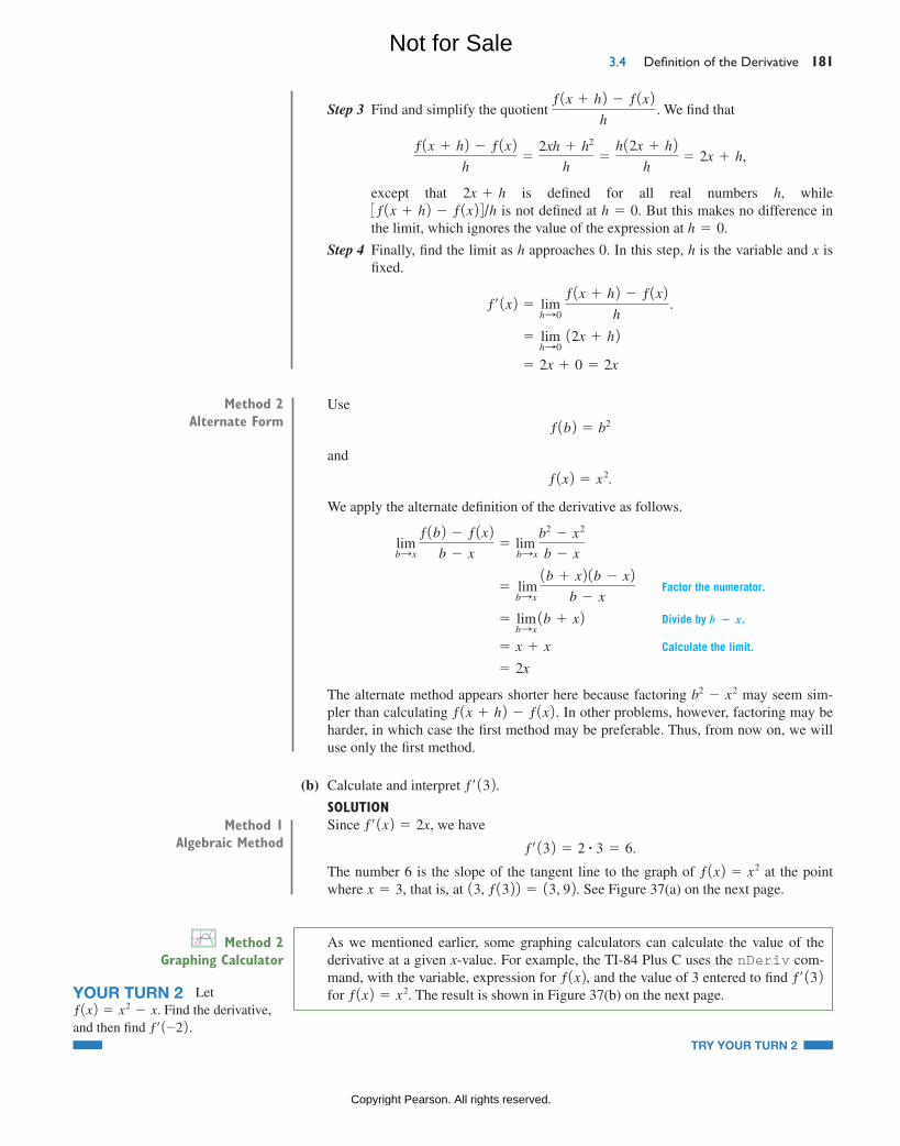
3.4 Definition of the Derivative 181
Step 3 Find and simplify the quotient ƒ1x + h2 - ƒ1x2
h . We find that
ƒ1x + h2 - ƒ1x2h
=2xh + h2
h=
h12x + h2h
= 2x + h,
except that 2x + h is defined for all real numbers h, while 3 ƒ1x + h2 - ƒ1x24/h is not defined at h = 0. But this makes no difference in the limit, which ignores the value of the expression at h = 0.
Step 4 Finally, find the limit as h approaches 0. In this step, h is the variable and x is fixed.
ƒ′1x2 = limhS0
ƒ1x + h2 - ƒ1x2
h .
= limhS0
12x + h2 = 2x + 0 = 2x
Use
ƒ1b2 = b2
and
ƒ1x2 = x2.
We apply the alternate definition of the derivative as follows.
lim bSx
ƒ1b2 - ƒ1x2b - x
= lim bSx
b2 - x2
b - x
= limbSx
1b + x21b - x2b - x
Factor the numerator.
= limbSx1b + x2 Divide by b − x.
= x + x Calculate the limit.
= 2x
The alternate method appears shorter here because factoring b2 - x2 may seem sim-pler than calculating ƒ1x + h2 - ƒ1x2. In other problems, however, factoring may be harder, in which case the first method may be preferable. Thus, from now on, we will use only the first method.
(b) Calculate and interpret ƒ′132.SolutionSince ƒ′1x2 = 2x, we have
ƒ′132 = 2 # 3 = 6.
The number 6 is the slope of the tangent line to the graph of ƒ1x2 = x2 at the point where x = 3, that is, at 13, ƒ1322 = 13, 92. See Figure 37(a) on the next page.
Method 2 alternate Form
Method 1 algebraic Method
As we mentioned earlier, some graphing calculators can calculate the value of the derivative at a given x-value. For example, the TI-84 Plus C uses the nDeriv com-mand, with the variable, expression for ƒ1x2, and the value of 3 entered to find ƒ′132 for ƒ1x2 = x2. The result is shown in Figure 37(b) on the next page.
Method 2 Graphing calculator
TRY YOUR TURN 2
YOUR TURN 2 Let ƒ1x2 = x2 - x. Find the derivative, and then find ƒ′1-22.
M03_LIAL8774_11_AIE_C03_133-208.indd 181 23/06/15 11:32 AM
Not for Sale
Copyright Pearson. All rights reserved.
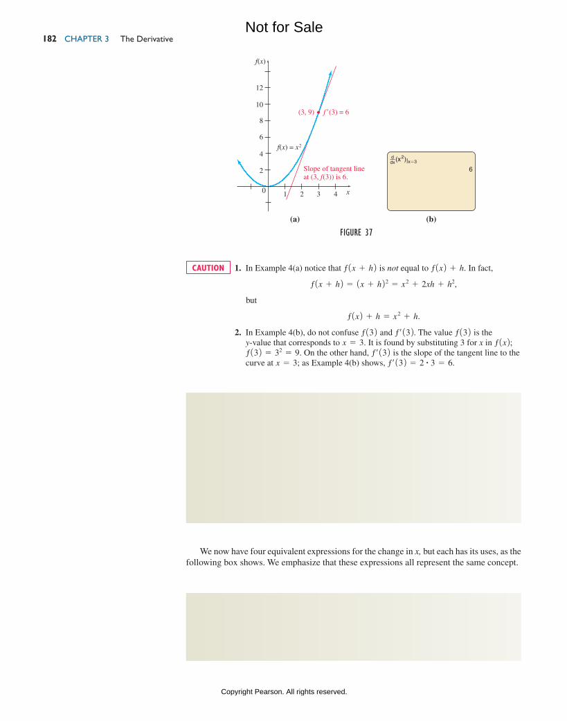
Chapter 3 the Derivative 182
1. In Example 4(a) notice that ƒ1x + h2 is not equal to ƒ1x2 + h. In fact,
ƒ1x + h2 = 1x + h22 = x2 + 2xh + h2,
but
ƒ1x2 + h = x2 + h.
2. In Example 4(b), do not confuse ƒ132 and ƒ′132. The value ƒ132 is the y-value that corresponds to x = 3. It is found by substituting 3 for x in ƒ1x2;ƒ132 = 32 = 9. On the other hand, ƒ′132 is the slope of the tangent line to the curve at x = 3; as Example 4(b) shows, ƒ′132 = 2 # 3 = 6.
Finding ƒ′ 1x 2 from the Definition of DerivativeThe four steps used to find the derivative ƒ′1x2 for a function y = ƒ1x2 are summarized here.
1. Find ƒ1x + h2. 2. Find and simplify ƒ1x + h2 - ƒ1x2.
3. Divide by h to get ƒ1x + h2 - ƒ1x2
h .
4. Let h S 0; ƒ′1x2 = limhS0
ƒ1x + h2 - ƒ1x2
h , if this limit exists.
We now have four equivalent expressions for the change in x, but each has its uses, as the following box shows. We emphasize that these expressions all represent the same concept.
Equivalent Expressions for the Change in xx2 - x1 Useful for describing the equation of a line through two pointsb - a A way to write x2 - x1 without the subscripts∆x Useful for describing the change in x without referring to the individual pointsh A way to write ∆x with just one symbol
caution
0 1 2 3 4
f(x)
x
6
10
4
8
12
2
f(x) = x2
Slope of tangent lineat (3, f(3)) is 6.
(a)
(3, 9) f ′(3) = 6
(x2)|x�3ddx
6
(b)
FigurE 37
M03_LIAL8774_11_AIE_C03_133-208.indd 182 03/07/15 12:31 PM
Not for Sale
Copyright Pearson. All rights reserved.
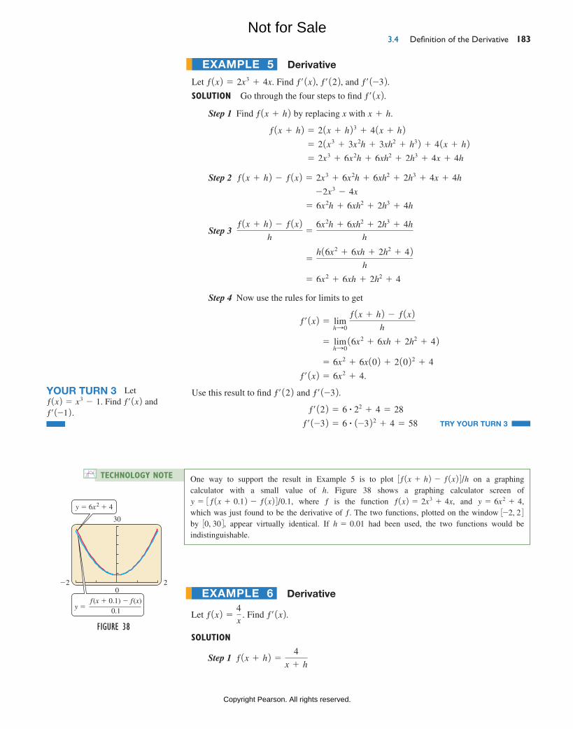
3.4 Definition of the Derivative 183
Derivative
Let ƒ1x2 = 2x3 + 4x. Find ƒ′1x2, ƒ′122, and ƒ′1-32.Solution Go through the four steps to find ƒ′1x2.
Step 1 Find ƒ1x + h2 by replacing x with x + h.
ƒ1x + h2 = 21x + h23 + 41x + h2 = 21x3 + 3x2h + 3xh2 + h32 + 41x + h2 = 2x3 + 6x2h + 6xh2 + 2h3 + 4x + 4h
Step 2 ƒ1x + h2 - ƒ1x2 = 2x3 + 6x2h + 6xh2 + 2h3 + 4x + 4h
= - 2x3 - 4x
= 6x2h + 6xh2 + 2h3 + 4h
Step 3 ƒ1x + h2 - ƒ1x2
h=
6x2h + 6xh2 + 2h3 + 4h
h
=h16x2 + 6xh + 2h2 + 42
h
= 6x2 + 6xh + 2h2 + 4
Step 4 Now use the rules for limits to get
ƒ′1x2 = limhS0
ƒ1x + h2 - ƒ1x2
h
= limhS016x2 + 6xh + 2h2 + 42
= 6x2 + 6x10² + 21022 + 4
ƒ′1x2 = 6x2 + 4.
Use this result to find ƒ′122 and ƒ′1-32. ƒ′122 = 6 # 22 + 4 = 28
ƒ′1-32 = 6 # 1-322 + 4 = 58 TRY YOUR TURN 3
ExampLE 5
YOUR TURN 3 Let ƒ1x2 = x3 - 1. Find ƒ′1x2 and ƒ′1-12.
technoloGy note One way to support the result in Example 5 is to plot 3ƒ1x + h2 - ƒ1x24/h on a graphing calculator with a small value of h. Figure 38 shows a graphing calculator screen of y = 3 ƒ1x + 0.12 - ƒ1x24/0.1, where ƒ is the function ƒ1x2 = 2x3 + 4x, and y = 6x2 + 4, which was just found to be the derivative of ƒ. The two functions, plotted on the window 3-2, 24 by 30, 304, appear virtually identical. If h = 0.01 had been used, the two functions would be indistinguishable.
�2 2
30
0
y � 6x2 � 4
y �f (x � 0.1) � f (x)
0.1
Figure 38
Derivative
Let ƒ1x2 =4x
. Find ƒ′1x2.
Solution
Step 1 ƒ1x + h2 =4
x + h
ExampLE 6
M03_LIAL8774_11_AIE_C03_133-208.indd 183 23/06/15 11:32 AM
Not for Sale
Copyright Pearson. All rights reserved.
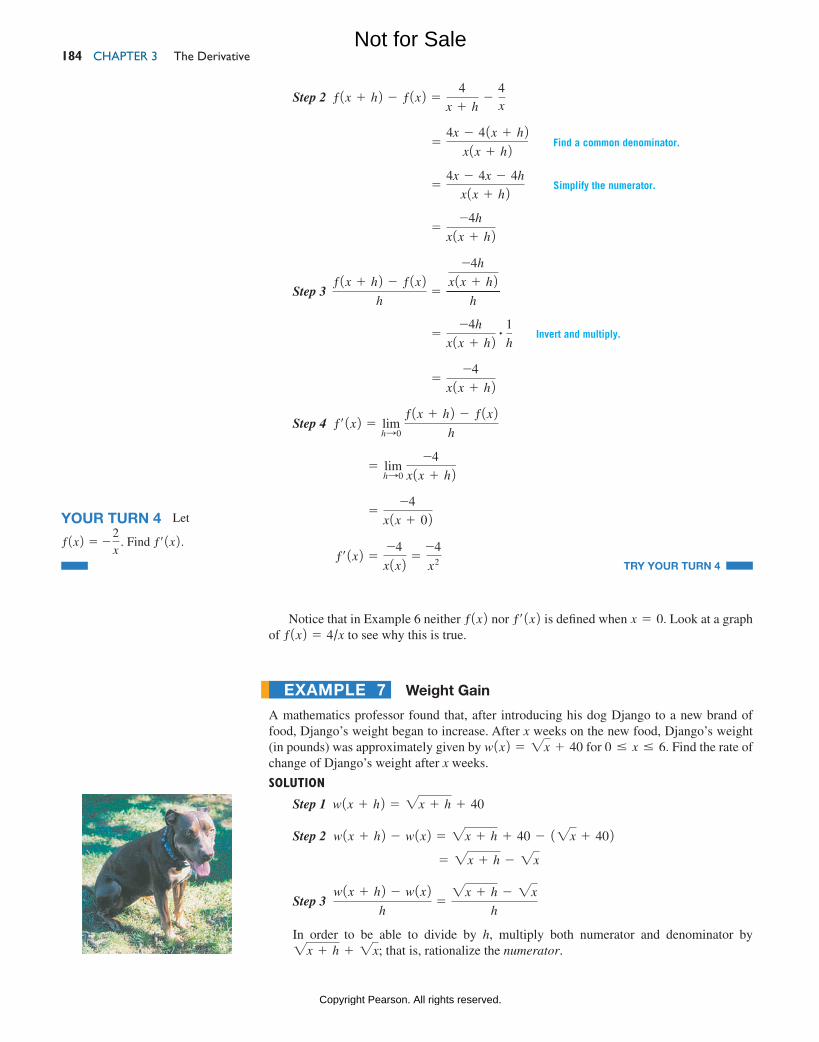
ChAptER 3 the Derivative 184
Step 2 ƒ1x + h2 - ƒ1x2 =4
x + h-
4x
=4x - 41x + h2
x1x + h2 Find a common denominator.
=4x - 4x - 4h
x1x + h2 Simplify the numerator.
=-4h
x1x + h2
Step 3 ƒ1x + h2 - ƒ1x2
h=
-4h
x1x + h2h
=-4h
x1x + h2# 1
h Invert and multiply.
=-4
x1x + h2
Step 4 ƒ′1x2 = limhS0
ƒ1x + h2 - ƒ1x2
h
= limhS0
-4
x1x + h2
=-4
x1x + 02
ƒ′1x2 =-4
x1x2 =-4
x2 TRY YOUR TURN 4
Notice that in Example 6 neither ƒ1x2 nor ƒ′1x2 is defined when x = 0. Look at a graph of ƒ1x2 = 4/x to see why this is true.
Weight Gain
A mathematics professor found that, after introducing his dog Django to a new brand of food, Django’s weight began to increase. After x weeks on the new food, Django’s weight (in pounds) was approximately given by w1x2 = 2x + 40 for 0 … x … 6. Find the rate of change of Django’s weight after x weeks.
Solution
Step 1 w1x + h2 = 2x + h + 40
Step 2 w1x + h2 - w1x2 = 2x + h + 40 - 12x + 402 = 2x + h - 2x
Step 3 w1x + h2 - w1x2
h=2x + h - 2x
h
In order to be able to divide by h, multiply both numerator and denominator by 2x + h + 2x; that is, rationalize the numerator.
ExampLE 7
YOUR TURN 4 Let
ƒ1x2 = - 2x
. Find ƒ′1x2.
M03_LIAL8774_11_AIE_C03_133-208.indd 184 23/06/15 11:33 AM
Not for Sale
Copyright Pearson. All rights reserved.
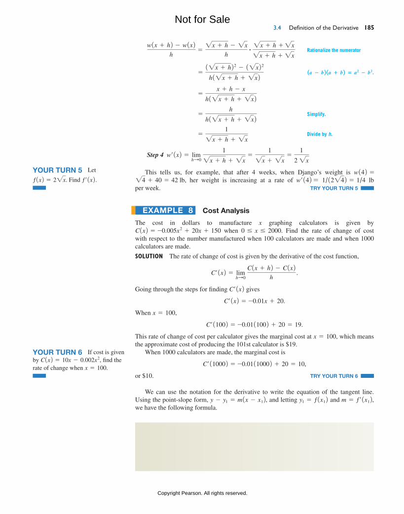
3.4 Definition of the Derivative 185
w1x + h2 - w1x2
h=2x + h - 2x
h# 2x + h + 2x2x + h + 2x
Rationalize the numerator
=12x + h22 - 12x22
h12x + h + 2x2 1a − b 2 1a + b 2 = a2 − b2.
=x + h - x
h12x + h + 2x2
=h
h12x + h + 2x2 Simplify.
=12x + h + 2x
Divide by h.
Step 4 w′1x2 = limhS0
12x + h + 2x
=12x + 2x
=1
2 2x
This tells us, for example, that after 4 weeks, when Django’s weight is w142 = 24 + 40 = 42 lb, her weight is increasing at a rate of w′142 = 1/12242 = 1/4 lb per week. TRY YOUR TURN 5
Cost analysis
The cost in dollars to manufacture x graphing calculators is given by C1x2 = -0.005x2 + 20x + 150 when 0 … x … 2000. Find the rate of change of cost with respect to the number manufactured when 100 calculators are made and when 1000 calculators are made.
Solution The rate of change of cost is given by the derivative of the cost function,
C′1x2 = limhS0
C1x + h2 - C1x2
h .
Going through the steps for finding C′1x2 gives
C′1x2 = -0.01x + 20.
When x = 100,
C′11002 = -0.0111002 + 20 = 19.
This rate of change of cost per calculator gives the marginal cost at x = 100, which means the approximate cost of producing the 101st calculator is $19.
When 1000 calculators are made, the marginal cost is
C′110002 = -0.01110002 + 20 = 10,
or $10. TRY YOUR TURN 6
We can use the notation for the derivative to write the equation of the tangent line. Using the point-slope form, y - y1 = m1x - x12, and letting y1 = ƒ1x12 and m = ƒ′1x12, we have the following formula.
equation of the tangent LineThe tangent line to the graph of y = ƒ1x2 at the point 1x1, ƒ1x122 is given by the equation
y − ƒ 1x1 2 = ƒ′ 1x1 2 1x − x1 2 ,provided ƒ′1x2 exists.
ExampLE 8
YOUR TURN 5 Let
ƒ1x2 = 22x. Find ƒ′1x2.
YOUR TURN 6 If cost is given by C1x2 = 10x - 0.002x2, find the rate of change when x = 100.
M03_LIAL8774_11_AIE_C03_133-208.indd 185 23/06/15 11:33 AM
Not for Sale
Copyright Pearson. All rights reserved.
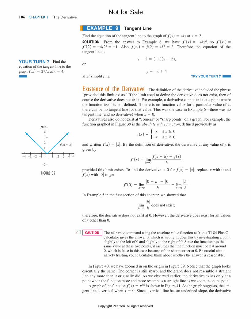
ChAptER 3 the Derivative 186
Tangent Line
Find the equation of the tangent line to the graph of ƒ1x2 = 4/x at x = 2.
Solution From the answer to Example 6, we have ƒ′1x2 = -4/x2, so ƒ′1x12 =ƒ′122 = -4/22 = -1. Also ƒ1x12 = ƒ122 = 4/2 = 2. Therefore the equation of the tangent line is
y - 2 = 1-121x - 22,or
y = -x + 4after simplifying. TRY YOUR TURN 7
existence of the Derivative The definition of the derivative included the phrase “provided this limit exists.” If the limit used to define the derivative does not exist, then of course the derivative does not exist. For example, a derivative cannot exist at a point where the function itself is not defined. If there is no function value for a particular value of x, there can be no tangent line for that value. This was the case in Example 6—there was no tangent line (and no derivative) when x = 0.
Derivatives also do not exist at “corners” or “sharp points” on a graph. For example, the function graphed in Figure 39 is the absolute value function, defined previously as
ƒ1x2 = b-x
-x
if x Ú 0
if x 6 0,
and written ƒ1x2 = 0 x 0 . By the definition of derivative, the derivative at any value of x is given by
ƒ′1x2 = limhS0
ƒ1x + h2 - ƒ1x2
h ,
provided this limit exists. To find the derivative at 0 for ƒ1x2 = 0 x 0 , replace x with 0 and ƒ1x2 with 00 0 to get
ƒ′102 = limhS0
00 + h 0 - 00 0
h= lim
hS0 0h 0h
.
In Example 5 in the first section of this chapter, we showed that
limhS0
0h 0h
does not exist;
therefore, the derivative does not exist at 0. However, the derivative does exist for all values of x other than 0.
The nDeriv command using the absolute value function at 0 on a TI-84 Plus C calculator gives the answer 0, which is wrong. It does this by investigating a point slightly to the left of 0 and slightly to the right of 0. Since the function has the same value at these two points, it assumes that the function must be flat around 0, which is false in this case because of the sharp corner at 0. Be careful about naively trusting your calculator; think about whether the answer is reasonable.
In Figure 40, we have zoomed in on the origin in Figure 39. Notice that the graph looks essentially the same. The corner is still sharp, and the graph does not resemble a straight line any more than it originally did. As we observed earlier, the derivative exists only at a point when the function more and more resembles a straight line as we zoom in on the point.
A graph of the function ƒ1x2 = x1/3 is shown in Figure 41. As the graph suggests, the tan-gent line is vertical when x = 0. Since a vertical line has an undefined slope, the derivative
ExampLE 9
caution
YOUR TURN 7 Find the equation of the tangent line to the graph ƒ1x2 = 22x at x = 4.
Figure 39
–2
2
1
4
3
42 31–2–3–4 –1 0 x
f(x)
f (x) = |x |
M03_LIAL8774_11_AIE_C03_133-208.indd 186 23/06/15 11:33 AM
Not for Sale
Copyright Pearson. All rights reserved.
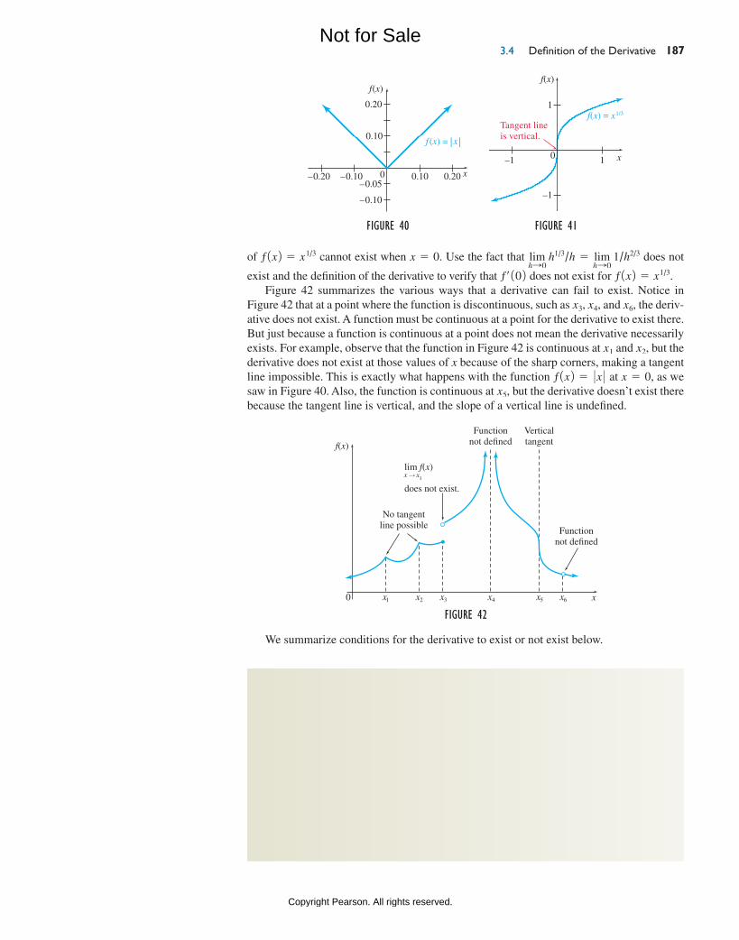
3.4 Definition of the Derivative 187
of ƒ1x2 = x1/3 cannot exist when x = 0. Use the fact that limhS0
h1/3/h = lim
hS0 1/h2/3 does not
exist and the definition of the derivative to verify that ƒ′102 does not exist for ƒ1x2 = x1/3.Figure 42 summarizes the various ways that a derivative can fail to exist. Notice in
Figure 42 that at a point where the function is discontinuous, such as x3, x4, and x6, the deriv-ative does not exist. A function must be continuous at a point for the derivative to exist there. But just because a function is continuous at a point does not mean the derivative necessarily exists. For example, observe that the function in Figure 42 is continuous at x1 and x2, but the derivative does not exist at those values of x because of the sharp corners, making a tangent line impossible. This is exactly what happens with the function ƒ1x2 = 0 x 0 at x = 0, as we saw in Figure 40. Also, the function is continuous at x5, but the derivative doesn’t exist there because the tangent line is vertical, and the slope of a vertical line is undefined.
Figure 40
–0.10
–0.05
0.10
0.20
0.200.10–0.10–0.20 0 x
f(x)
f (x) = |x |
Figure 41
0 1
1
–1
–1
f(x)
x
f(x) = x1/3
Tangent lineis vertical.
Figure 42
f(x)
0 x x x x x x x1 2 3 4 5 6
Functionnot de�ned
Verticaltangent
Functionnot de�ned
No tangentline possible
lim f(x)
does not exist.3x x
We summarize conditions for the derivative to exist or not exist below.
existence of the DerivativeThe derivative exists when a function ƒ satisfies all of the following conditions at a point.
1. ƒ is continuous,
2. ƒ is smooth, and
3. ƒ does not have a vertical tangent line.
The derivative does not exist when any of the following conditions are true for a function at a point.
1. ƒ is discontinuous,
2. ƒ has a sharp corner, or
3. ƒ has a vertical tangent line.
M03_LIAL8774_11_AIE_C03_133-208.indd 187 23/06/15 11:33 AM
Not for Sale
Copyright Pearson. All rights reserved.
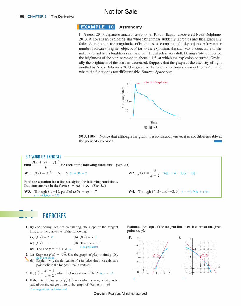
ChAptER 3 the Derivative 188
astronomy
In August 2013, Japanese amateur astronomer Koichi Itagaki discovered Nova Delphinus 2013. A nova is an exploding star whose brightness suddenly increases and then gradually fades. Astronomers use magnitudes of brightness to compare night sky objects. A lower star number indicates brighter objects. Prior to the explosion, the star was undetectable to the naked eye and had a brightness measure of +17, which is very dull. During a 24-hour period the brightness of the star increased to about +4.5, at which the explosion occurred. Gradu-ally the brightness of the star has decreased. Suppose that the graph of the intensity of light emitted by Nova Delphinus 2013 is given as the function of time shown in Figure 43. Find where the function is not differentiable. Source: Space.com.
ExampLE 10
Figure 43
4
8
12
16
Vis
ual m
agni
tude
Point of explosion
Timet
Solution Notice that although the graph is a continuous curve, it is not differentiable at the point of explosion.
Find ƒ 1x + h 2 − ƒ 1x 2
h for each of the following functions. (Sec. 2.1)
3.4 warm-up exercises
W1. ƒ1x2 = 3x2 - 2x - 5 6x + 3h - 2 W2. ƒ1x2 =3
x - 2 -3/31x + h - 221x - 224
Find the equation for a line satisfying the following conditions. Put your answer in the form y = mx + b. (Sec. 1.1)
W3. Through 14, -12, parallel to 5x + 6y = 7 W4. Through 16, 22 and 1-2, 52 y = -13/82 x + 17/4y = -15/62x + 7/3
1. By considering, but not calculating, the slope of the tangent line, give the derivative of the following.
(a) ƒ1x2 = 5 0 (b) ƒ1x2 = x 1
(c) ƒ1x2 = -x -1 (d) The line x = 3
(e) The line y = mx + b m
2. (a) Suppose g1x2 = 23 x . Use the graph of g1x2 to find g′102.(b) Explain why the derivative of a function does not exist at a
point where the tangent line is vertical.
3. If ƒ1x2 =x2 - 1
x + 2 , where is ƒ not differentiable? At x = -2
4. If the rate of change of ƒ1x2 is zero when x = a, what can be said about the tangent line to the graph of ƒ1x2 at x = a?
3.4 exercisesEstimate the slope of the tangent line to each curve at the given point 1x, y 2 .
Does not exist
Does not exist
The tangent line is horizontal.
5.
0 2 4 6
4
y
x
6
2
(5, 3)
6. y
–2
2
4
2–2 0 x
(2, 2)
2 -1
M03_LIAL8774_11_AIE_C03_133-208.indd 188 23/06/15 11:33 AM
Not for Sale
Copyright Pearson. All rights reserved.
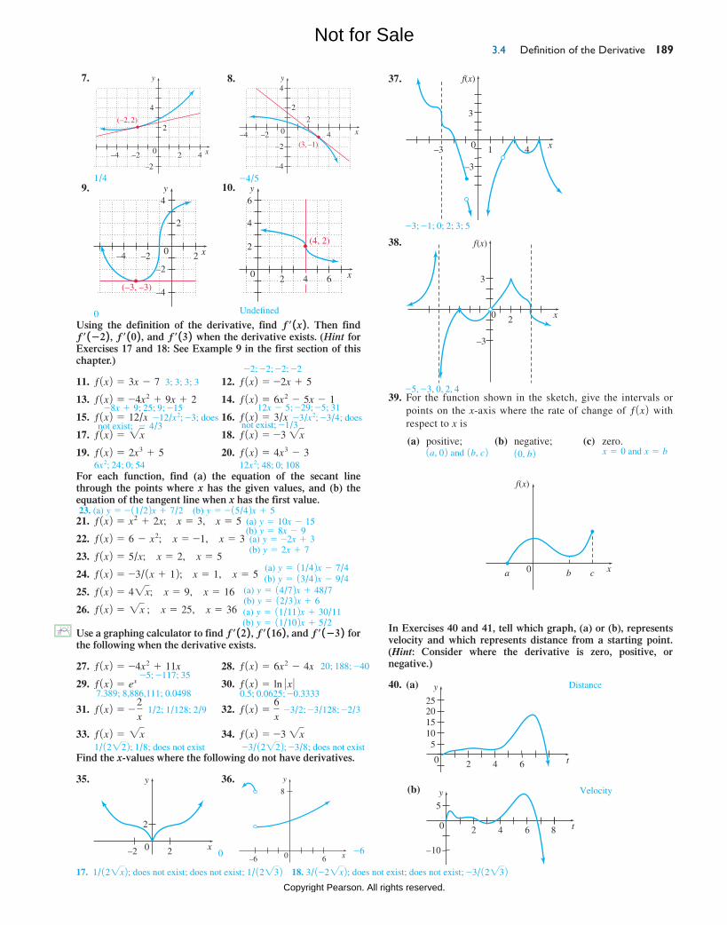
3.4 Definition of the Derivative 189
Using the definition of the derivative, find ƒ′ 1x 2 . Then find ƒ′ 1−2 2 , ƒ′ 10 2 , and ƒ′ 13 2 when the derivative exists. (Hint for Exercises 17 and 18: See Example 9 in the first section of this chapter.)
11. ƒ1x2 = 3x - 7 3; 3; 3; 3 12. ƒ1x2 = -2x + 5
13. ƒ1x2 = -4x2 + 9x + 2 14. ƒ1x2 = 6x2 - 5x - 1
15. ƒ1x2 = 12/x 16. ƒ1x2 = 3/x 17. ƒ1x2 = 2x 18. ƒ1x2 = -3 2x
19. ƒ1x2 = 2x3 + 5 20. ƒ1x2 = 4x3 - 3
For each function, find (a) the equation of the secant line through the points where x has the given values, and (b) the equation of the tangent line when x has the first value.
21. ƒ1x2 = x2 + 2x; x = 3, x = 5
22. ƒ1x2 = 6 - x2; x = -1, x = 3
23. ƒ1x2 = 5/x; x = 2, x = 5
24. ƒ1x2 = -3/1x + 12; x = 1, x = 5
25. ƒ1x2 = 42x; x = 9, x = 16
26. ƒ1x2 = 2x ; x = 25, x = 36
Use a graphing calculator to find ƒ′ 12 2 , ƒ′ 116 2 , and ƒ′ 1−3 2 for the following when the derivative exists.
27. ƒ1x2 = -4x2 + 11x 28. ƒ1x2 = 6x2 - 4x
29. ƒ1x2 = ex 30. ƒ1x2 = ln 0 x 0 31. ƒ1x2 = -
2x 1/2; 1/128; 2/9 32. ƒ1x2 =
6x -3/2; -3/128; -2/3
33. ƒ1x2 = 2x 34. ƒ1x2 = -3 2x
Find the x-values where the following do not have derivatives.
35. y
0 x2
2
–2
36. y
8
6–6 0 x
7. y
–2
4
2
2 4–2–4 0 x
(–2, 2)
8. y
–2
–4
4
2
2
–2 4–4 0 x
(3, –1)
37.
0 41–3
–3
f(x)
x
3
38.
0 2
–3
f(x)
x
3
39. For the function shown in the sketch, give the intervals or points on the x-axis where the rate of change of ƒ1x2 with respect to x is
(a) positive; (b) negative; (c) zero.
1/4 -4/5 9. y
–2
–4
4
2
2–2–4 0 x
(–3, –3)
10. y
2
6
4
62 40 x
(4, 2)
0 Undefined
-2; -2; -2; -2
-8x + 9; 25; 9; -15 12x - 5; -29; -5; 31-12/x2; -3; does -3/x2; -3/4; does
12x2; 48; 0; 1086x2; 24; 0; 54
not exist; -1/3not exist; - 4/3
(a) y = 10x - 15(b) y = 8x - 9(a) y = -2x + 3(b) y = 2x + 7
(a) y = 11/42x - 7/4(b) y = 13/42x - 9/4
(a) y = 14/72x + 48/7(b) y = 12/32x + 6(a) y = 11/112x + 30/11(b) y = 11/102x + 5/2
-5; -117; 3520; 188; -40
7.389; 8,886,111; 0.0498 0.5; 0.0625; -0.3333
1/12222; 1/8; does not exist -3/12222; -3/8; does not exist
0 -6
-3; -1; 0; 2; 3; 5
-5, -3, 0, 2, 4
1a, 02 and 1b, c2 10, b2 x = 0 and x = b
f(x)
b ca 0 x
In Exercises 40 and 41, tell which graph, (a) or (b), represents velocity and which represents distance from a starting point. (Hint: Consider where the derivative is zero, positive, or negative.)
40. (a)
0 2 4 6
510152025
y
t
(b)
5
y
0 2 4 6 8
–10
t
Distance
Velocity
17. 1/122x2; does not exist; does not exist; 1/12232 18. 3/1-22x2; does not exist; does not exist; -3/12232
23. (a) y = -11/22x + 7/2 (b) y = -15/42x + 5
M03_LIAL8774_11_AIE_C03_133-208.indd 189 03/07/15 9:47 AM
Not for Sale
Copyright Pearson. All rights reserved.
ChAptER 3 the Derivative 190
41. (a)
0 2 4 8
40302010
y
t
(b)
0 2 6 8
302010
y
t
In Exercises 42–45, find the derivative of the function at the given point.
(a) Approximate the definition of the derivative with small values of h.
(b) Use a graphing calculator to zoom in on the function until it appears to be a straight line, and then find the slope of that line.
42. ƒ1x2 = xx; a = 2 6.773 43. ƒ1x2 = xx; a = 3 56.66
44. ƒ1x2 = x1/x; a = 2 0.1085 45. ƒ1x2 = x1/x; a = 3
46. For each function in Column A, graph 3ƒ1x + h2 - ƒ1x24/h for a small value of h on the window 3-2, 24 by 3-2, 84 . Then graph each function in Column B on the same window. Compare the first set of graphs with the second set to choose from Column B the derivative of each of the functions in Column A.
Column A Column B
ln 0 x 0 ex
ex 3x2
x3 1x
47. Explain whyƒ1x + h2 - ƒ1x - h2
2h should give a reasonable approximation of ƒ′1x2 when ƒ′1x2
exists and h is small.
48. (a) For the function ƒ1x2 = -4x2 + 11x, find the value of ƒ′132, as well as the approximation using
ƒ1x + h2 - ƒ1x2h
and using the formula in Exercise 47 with h = 0.1.
(b) Repeat part (a) using h = 0.01. -13.04, -13
(c) Repeat part (a) using the function ƒ1x2 = -2/x and h = 0.1.
(d) Repeat part (c) using h = 0.01. 0.221484, 0.222225
(e) Repeat part (a) using the function ƒ1x2 = 2x and h = 0.1.
(f) Repeat part (e) using h = 0.01. 0.288435, 0.288676
(g) Using the results of parts (a) through (f), discuss which approximation formula seems to give better accuracy.
appLicationsBusiness and Economics 49. Demand Suppose the demand for a certain item is given by
D1p2 = -2p2 - 4p + 300, where p represents the price of the item in dollars.
(a) Find the rate of change of demand with respect to price. -4p - 4
(b) Find and interpret the rate of change of demand when the price is $10.
50. Profit The profit (in thousands of dollars) from the expen-diture of x thousand dollars on advertising is given by P1x2 =1000 + 32x - 2x2. Find the marginal profit at the following expenditures. In each case, decide whether the firm should increase the expenditure.
(a) $8000 (b) $6000 (c) $12,000 (d) $20,000
51. Revenue The revenue in dollars generated from the sale of x
picnic tables is given by R1x2 = 20x -x2
500 .
(a) Find the marginal revenue when 1000 tables are sold.
(b) Estimate the revenue from the sale of the 1001st table by finding R′110002. $16
(c) Determine the actual revenue from the sale of the 1001st table. $15.998 (or $16)
(d) Compare your answers for parts (b) and (c). What do you find? The marginal revenue gives a good approximation of the actual revenue from the sale of the 1001st table.
52. cost The cost in dollars of producing x tacos is C1x2 = -0.00375x2 + 1.5x + 1000, for 0 … x … 180.
(a) Find the marginal cost.
(b) Find and interpret the marginal cost at a production level of 100 tacos. $0.75
(c) Find the exact cost to produce the 101st taco. $0.74625
(d) Compare the answers to parts (b) and (c). How are they related? They are very close.
(e) Show that whenever C1x2 = ax2 + bx + c, 3C1x + 12 - C1x24 - C′1x2 = a. Source: The College
Mathematics Journal.
(f) Show that whenever C1x2 = ax2 + bx + c,
C1x + 12 - C1x2 = C′ax +1
2b.
53. Social Security assets The table on the next page gives actual and projected year-end assets in Social Security trust funds, in trillions of current dollars, where Year represents the number of years since 2000. The polynomial function defined by
ƒ1x2 = 0.0000329x3 - 0.00450x2 + 0.0613x + 2.34
models the data quite well. Source: Social Security Administration.
(a) To verify the fit of the model, find ƒ1102, ƒ1202, and ƒ1302. 2.54; 2.03; 1.02
(b) Use a graphing calculator with a command such as nDeriv to find the slope of the tangent line to the graph of ƒ at the following x-values: 0, 10, 20, 30, and 35.
Distance
Velocity
-0.0158
The derivative of ln x is 1/x, the derivative of ex is ex, and the derivative of x3 is 3x2.
-13, -13.4, -13
0.222222, 0.215054, 0.222469
0.288675, 0.286309, 0.288715
-44; demand is decreasing at a rate of about 44 items for each increase in price of $1.
$0; no $8000; yes -$16,000; no -$48,000; no
$16 per table
C>1x2 = -0.0075x + 1.5, 0 … x … 180
Answers are in trillions of dollars.
0.061; -0.019; -0.079; -0.120; -0.133
M03_LIAL8774_11_AIE_C03_133-208.indd 190 23/06/15 11:33 AM
Not for Sale
Copyright Pearson. All rights reserved.
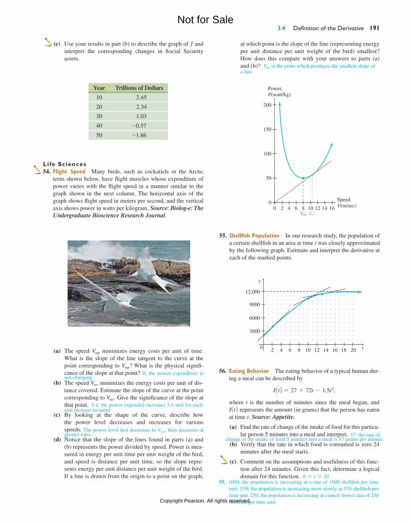
3.4 Definition of the Derivative 191
Life Sciences 54. Flight Speed Many birds, such as cockatiels or the Arctic
terns shown below, have flight muscles whose expenditure of power varies with the flight speed in a manner similar to the graph shown in the next column. The horizontal axis of the graph shows flight speed in meters per second, and the vertical axis shows power in watts per kilogram. Source: Biolog-e: The Undergraduate Bioscience Research Journal.
55. Shellfish Population In one research study, the population of a certain shellfish in an area at time t was closely approximated by the following graph. Estimate and interpret the derivative at each of the marked points.
(a) The speed Vmp minimizes energy costs per unit of time. What is the slope of the line tangent to the curve at the point corresponding to Vmp? What is the physical signifi-cance of the slope at that point?
(b) The speed Vmr minimizes the energy costs per unit of dis-tance covered. Estimate the slope of the curve at the point corresponding to Vmr. Give the significance of the slope at that point.
(c) By looking at the shape of the curve, describe how the power level decreases and increases for various speeds.
(d) Notice that the slope of the lines found in parts (a) and (b) represents the power divided by speed. Power is mea-sured in energy per unit time per unit weight of the bird, and speed is distance per unit time, so the slope repre-sents energy per unit distance per unit weight of the bird. If a line is drawn from the origin to a point on the graph,
146 124
150
100
200
50
01610820
SpeedV(m/sec)
Vmp Vmr
Power,P(watt/kg)
9000
12,000
6000
3000
2 64 108 14 1612 18 20 t
y
0
56. eating Behavior The eating behavior of a typical human dur-ing a meal can be described by
I1t2 = 27 + 72t - 1.5t2,
where t is the number of minutes since the meal began, and I1t2 represents the amount (in grams) that the person has eaten at time t. Source: Appetite.
(a) Find the rate of change of the intake of food for this particu-lar person 5 minutes into a meal and interpret.
(b) Verify that the rate in which food is consumed is zero 24 minutes after the meal starts.
(c) Comment on the assumptions and usefulness of this func-tion after 24 minutes. Given this fact, determine a logical domain for this function. 0 … t … 24
55. 1000; the population is increasing at a rate of 1000 shellfish per time unit. 570; the population is increasing more slowly at 570 shellfish per time unit. 250; the population is increasing at a much slower rate of 250 shellfish per time unit.
57, the rate of change of the intake of food 5 minutes into a meal is 57 grams per minute.
0, the power expenditure is not changing.
5.4, the power expended increases 5.4 unit for each unit increase in speed
The power level first decreases to Vmp, then increases at greater rates.
(c) Use your results in part (b) to describe the graph of ƒ and interpret the corresponding changes in Social Security assets.
Year Trillions of Dollars
10 2.45
20 2.34
30 1.03
40 -0.57
50 -1.86
at which point is the slope of the line (representing energy per unit distance per unit weight of the bird) smallest? How does this compare with your answers to parts (a) and (b)? Vmr is the point which produces the smallest slope of a line.
M03_LIAL8774_11_AIE_C03_133-208.indd 191 23/06/15 11:33 AM
Not for Sale
Copyright Pearson. All rights reserved.
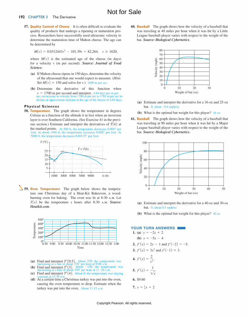
ChAptER 3 the Derivative 192
60. Baseball The graph shows how the velocity of a baseball that was traveling at 40 miles per hour when it was hit by a Little League baseball player varies with respect to the weight of the bat. Source: Biological Cybernetics.
At 500 ft, the temperature decreases 0.005° per
T (ºC)
252015105
7000500030001000 9000 h (ft)
T = T(h)
foot. At about 1500 ft, the temperature increases 0.008° per foot. At 5000 ft, the temperature decreases 0.00125° per foot.
59. oven temperature The graph below shows the tempera-ture one Christmas day of a Heat-Kit Bakeoven, a wood- burning oven for baking. The oven was lit at 8:30 a.m. Let T1x2 be the temperature x hours after 8:30 a.m. Source: Heatkit.com.
8:300º
100º200º300º400º500º
9:309:00 10:00 10:30 11:00 11:30 12:00 12:30 1:00
Tem
pera
ture
Time
70
30
60
20
50
80
40
100
100 20 30Weight of bat (oz)
Vel
ocity
(m
ph)
80
60
20
100
40
020 40100 30 50
Weight of bat (oz)
Vel
ocity
(m
ph)
(a) Estimate and interpret the derivative for a 16-oz and 25-oz bat. 0; about -0.6 mph/oz
(b) What is the optimal bat weight for this player? 16 oz
61. Baseball The graph shows how the velocity of a baseball that was traveling at 90 miles per hour when it was hit by a Major League baseball player varies with respect to the weight of the bat. Source: Biological Cybernetics.
(a) Estimate and interpret the derivative for a 40-oz and 30-oz bat. 0; about 0.5 mph/oz
(b) What is the optimal bat weight for this player? 40 oz
YOUR TURN aNSWERS 1. (a) y = -2x + 2
(b) y = -5x - 4
2. ƒ′1x2 = 2x - 1 and ƒ′1-22 = -5.
3. ƒ′1x2 = 3x2 and ƒ′1-12 = 3.
4. ƒ′1x2 =2
x2 .
5. ƒ′1x2 =12x
6. $9.60
7. y = 12 x + 2
57. Quality control of cheese It is often difficult to evaluate the quality of products that undergo a ripening or maturation pro-cess. Researchers have successfully used ultrasonic velocity to determine the maturation time of Mahon cheese. The age can be determined by
M1v2 = 0.0312443v2 - 101.39v + 82,264, v Ú 1620,
where M1v2 is the estimated age of the cheese (in days) for a velocity v (m per second). Source: Journal of Food Science.
(a) If Mahon cheese ripens in 150 days, determine the velocity of the ultrasound that one would expect to measure. (Hint: Set M1v2 = 150 and solve for v.) 1690 m per sec
(b) Determine the derivative of this function when v = 1700 m per second and interpret.
Physical Sciences 58. temperature The graph shows the temperature in degrees
Celsius as a function of the altitude h in feet when an inversion layer is over Southern California. (See Exercise 41 in the previ-ous section.) Estimate and interpret the derivatives of T1h2 at the marked points.
4.84 days per m per sec; an increase in velocity from 1700 m per sec to 1701 m per sec in-dicates an approximate increase in the age of the cheese of 4.84 days.
About 270; the temperature was increasing at a rate of about 270° per hour at 9:00 a.m.
About -150; the temperature was decreasing at a rate of about 150° per hour at 11 :30 a.m.
About 0; the temperature was staying constant at 12:30 p.m.
(a) Find and interpret T′10.52.(b) Find and interpret T′132.(c) Find and interpret T′142.(d) At a certain time a Christmas turkey was put into the oven,
causing the oven temperature to drop. Estimate when the turkey was put into the oven. About 11:15 a.m.
M03_LIAL8774_11_AIE_C03_133-208.indd 192 23/06/15 11:33 AM
Not for Sale
Copyright Pearson. All rights reserved.
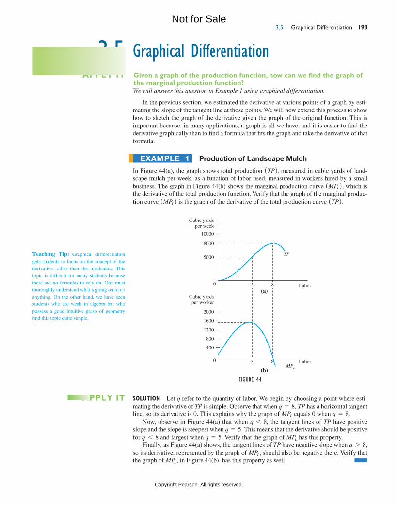
3.5 Graphical Differentiation 193
We will answer this question in Example 1 using graphical differentiation.
In the previous section, we estimated the derivative at various points of a graph by esti-mating the slope of the tangent line at those points. We will now extend this process to show how to sketch the graph of the derivative given the graph of the original function. This is important because, in many applications, a graph is all we have, and it is easier to find the derivative graphically than to find a formula that fits the graph and take the derivative of that formula.
production of Landscape mulch
In Figure 44(a), the graph shows total production 1TP2, measured in cubic yards of land-scape mulch per week, as a function of labor used, measured in workers hired by a small business. The graph in Figure 44(b) shows the marginal production curve 1MPL2, which is the derivative of the total production function. Verify that the graph of the marginal produc-tion curve 1MPL2 is the graph of the derivative of the total production curve 1TP2.
ExampLE 1
graphical DifferentiationGiven a graph of the production function, how can we find the graph of the marginal production function?
APPLY IT
3.5
Teaching Tip: Graphical differentiation gets students to focus on the concept of the derivative rather than the mechanics. This topic is difficult for many students because there are no formulas to rely on. One must thoroughly understand what’s going on to do anything. On the other hand, we have seen students who are weak in algebra but who possess a good intuitive grasp of geometry find this topic quite simple.
Figure 44
Cubic yardsper week
2000
800
1200
1600
0
400
85 LaborMPL
Cubic yardsper worker
10000
8000
0
5000
85 Labor
TP
(a)
(b)
Solution Let q refer to the quantity of labor. We begin by choosing a point where esti-mating the derivative of TP is simple. Observe that when q = 8, TP has a horizontal tangent line, so its derivative is 0. This explains why the graph of MPL equals 0 when q = 8.
Now, observe in Figure 44(a) that when q 6 8, the tangent lines of TP have positive slope and the slope is steepest when q = 5. This means that the derivative should be positive for q 6 8 and largest when q = 5. Verify that the graph of MPL has this property.
Finally, as Figure 44(a) shows, the tangent lines of TP have negative slope when q 7 8, so its derivative, represented by the graph of MPL, should also be negative there. Verify that the graph of MPL, in Figure 44(b), has this property as well.
APPLY IT
M03_LIAL8774_11_AIE_C03_133-208.indd 193 23/06/15 11:33 AM
Not for Sale
Copyright Pearson. All rights reserved.
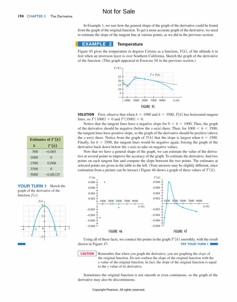
ChAptER 3 the Derivative 194
In Example 1, we saw how the general shape of the graph of the derivative could be found from the graph of the original function. To get a more accurate graph of the derivative, we need to estimate the slope of the tangent line at various points, as we did in the previous section.
Temperature
Figure 45 gives the temperature in degrees Celsius as a function, T1h2, of the altitude h in feet when an inversion layer is over Southern California. Sketch the graph of the derivative of the function. (This graph appeared in Exercise 58 in the previous section.)
ExampLE 2
Estimates of T′ 1h 2h T′ 1h 2
500 -0.005
1000 0
1500 0.008
3500 0
5000 -0.00125
Figure 45
T (ºC)
252015105
7000500030001000 9000 h (ft)
T = T(h)
Solution First, observe that when h = 1000 and h = 3500, T1h2 has horizontal tangent lines, so T′110002 = 0 and T′135002 = 0.
Notice that the tangent lines have a negative slope for 0 6 h 6 1000. Thus, the graph of the derivative should be negative (below the x-axis) there. Then, for 1000 6 h 6 3500, the tangent lines have positive slope, so the graph of the derivative should be positive (above the x-axis) there. Notice from the graph of T1h2 that the slope is largest when h = 1500. Finally, for h 7 3500, the tangent lines would be negative again, forcing the graph of the derivative back down below the x-axis to take on negative values.
Now that we have a general shape of the graph, we can estimate the value of the deriva-tive at several points to improve the accuracy of the graph. To estimate the derivative, find two points on each tangent line and compute the slope between the two points. The estimates at selected points are given in the table to the left. (Your answers may be slightly different, since estimation from a picture can be inexact.) Figure 46 shows a graph of these values of T′1h2.
T′(h)
0.008
0.006
0.004
0.002
–0.002
–0.004
–0.006
–0.008
50001000 3000 7000 9000
h (ft)
Figure 46
T′(h)
0.008
0.006
0.004
0.002
–0.002
–0.004
–0.006
–0.008
50001000 3000 7000 9000
h (ft)
Figure 47
Using all of these facts, we connect the points in the graph T′1h2 smoothly, with the result shown in Figure 47. TRY YOUR TURN 1
YOUR TURN 1 Sketch the graph of the derivative of the function ƒ1x2.
–2
2
4
42–2–4 0 x
f(x)
Remember that when you graph the derivative, you are graphing the slope of the original function. Do not confuse the slope of the original function with the y-value of the original function. In fact, the slope of the original function is equal to the y-value of its derivative.
Sometimes the original function is not smooth or even continuous, so the graph of the derivative may also be discontinuous.
caution
M03_LIAL8774_11_AIE_C03_133-208.indd 194 23/06/15 11:33 AM
Not for Sale
Copyright Pearson. All rights reserved.
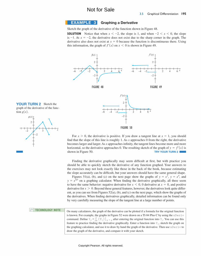
3.5 Graphical Differentiation 195
Graphing a Derivative
Sketch the graph of the derivative of the function shown in Figure 48.
Solution Notice that when x 6 -2, the slope is 1, and when -2 6 x 6 0, the slope is -1. At x = -2, the derivative does not exist due to the sharp corner in the graph. The derivative also does not exist at x = 0 because the function is discontinuous there. Using this information, the graph of ƒ′1x2 on x 6 0 is shown in Figure 49.
ExamplE 3
Figure 48
–2
f(x)
2 4 6–6 –4 –2 x
2
Figure 49
–2
f ′(x)
2 4 6–6 –2–4 x
2
Figure 50
–2
f ′(x)
2 4 6–6 –2–4 x
2
For x 7 0, the derivative is positive. If you draw a tangent line at x = 1, you should find that the slope of this line is roughly 1. As x approaches 0 from the right, the derivative becomes larger and larger. As x approaches infinity, the tangent lines become more and more horizontal, so the derivative approaches 0. The resulting sketch of the graph of y = ƒ′1x2 is shown in Figure 50. TRY YOUR TURN 2
YOUR TURN 2 Sketch the graph of the derivative of the func-tion g1x2.
–2
g(x)
3–2 x
2
technology note On many calculators, the graph of the derivative can be plotted if a formula for the original function is known. For example, the graphs in Figure 52 were drawn on a TI-84 Plus C by using the nDeriv command. Define Y2 = (Y1) 0 x = x after entering the original function into Y1. You can use this feature to practice finding the derivative graphically. Enter a function into Y1, sketch the graph on the graphing calculator, and use it to draw by hand the graph of the derivative. Then use nDeriv to draw the graph of the derivative, and compare it with your sketch.
d dx
Finding the derivative graphically may seem difficult at first, but with practice you should be able to quickly sketch the derivative of any function graphed. Your answers to the exercises may not look exactly like those in the back of the book, because estimating the slope accurately can be difficult, but your answers should have the same general shape.
Figures 51(a), (b), and (c) on the next page show the graphs of y = x2, y = x4, and y = x4/3 on a graphing calculator. When finding the derivative graphically, all three seem to have the same behavior: negative derivative for x 6 0, 0 derivative at x = 0, and positive derivative for x 7 0. Beyond these general features, however, the derivatives look quite differ-ent, as you can see from Figures 52(a), (b), and (c) on the next page, which show the graphs of the derivatives. When finding derivatives graphically, detailed information can be found only by very carefully measuring the slope of the tangent line at a large number of points.
M03_LIAL8774_11_AIE_C03_133-208.indd 195 03/07/15 9:50 AM
Not for Sale
Copyright Pearson. All rights reserved.
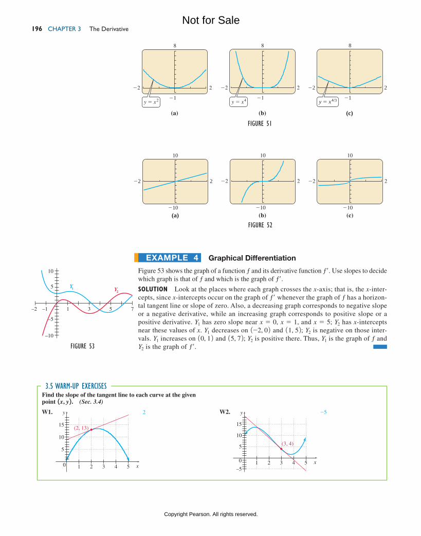
ChAptER 3 the Derivative 196
Figure 52
22 2
10
210(a)
22 2
10
210
(b)
22 2
10
210
(c)
Graphical Differentiation
Figure 53 shows the graph of a function ƒ and its derivative function ƒ′. Use slopes to decide which graph is that of ƒ and which is the graph of ƒ′.Solution Look at the places where each graph crosses the x-axis; that is, the x-inter-cepts, since x-intercepts occur on the graph of ƒ′ whenever the graph of ƒ has a horizon-tal tangent line or slope of zero. Also, a decreasing graph corresponds to negative slope or a negative derivative, while an increasing graph corresponds to positive slope or a positive derivative. Y1 has zero slope near x = 0, x = 1, and x = 5; Y2 has x-intercepts near these values of x. Y1 decreases on 1-2, 02 and 11, 52; Y2 is negative on those inter-vals. Y1 increases on 10, 12 and 15, 72; Y2 is positive there. Thus, Y1 is the graph of ƒ and Y2 is the graph of ƒ′.
ExampLE 4
Figure 53
1 3 5 7–2 –1
–10
–5
5
10
Y1 Y2
Find the slope of the tangent line to each curve at the given point 1x, y 2 . (Sec. 3.4)
3.5 warm-up exercises
W1.
0 1
y
x
5
(2, 13)
10
15
2 3 4 5
2 W2.
(3, 4)
0 1
y
x
5
10
–5
15
2 3 4 5
-5
Figure 51
22 2
8
21y 5 x2
(a)
22 2
8
21y 5 x4
(b)
22 2
8
21y 5 x4/3
(c)
M03_LIAL8774_11_AIE_C03_133-208.indd 196 23/06/15 11:33 AM
Not for Sale
Copyright Pearson. All rights reserved.
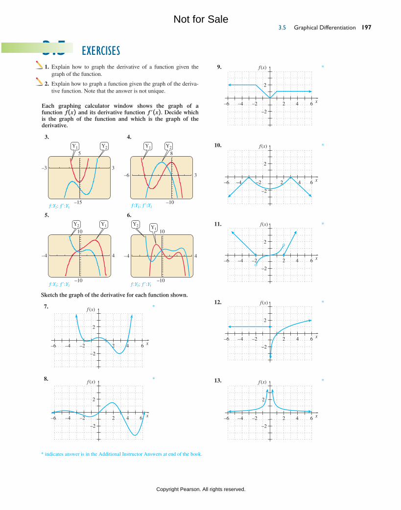
3.5 Graphical Differentiation 197
3.5 exercises 1. Explain how to graph the derivative of a function given the
graph of the function.
2. Explain how to graph a function given the graph of the deriva-tive function. Note that the answer is not unique.
9.
–2
(x)
2 4 6–6 –2–4 x
2
f *
10.
–2
4 6–6 –2–4 x
2
(x)f
2
*
11.
–2
(x)
2–2 4 6–6 –4 x
2
f *
12.
–2
(x)
2–2 4 6–6 –4 x
2
f *
13.
–2
(x)
2 4 6–6 –2–4 x
2
f *
7.
–2
(x)
2 4 6–6 –4 –2 x
2
f *
8.
–2
f(x)
2 4 6–6 –4 –2 x
2
f *
Sketch the graph of the derivative for each function shown.
ƒ:Y2; ƒ′:Y1 ƒ:Y1; ƒ′:Y2
ƒ:Y1; ƒ′:Y2 ƒ:Y2; ƒ′:Y1
* indicates answer is in the Additional Instructor Answers at end of the book.
3.
Y1 Y2
5
–15
–3 3
4.
Y1 Y2
8
–10
–6 3
5.
Y1Y2
10
–10
–4 4
6.
Y1Y2
10
–10
–4 4
Each graphing calculator window shows the graph of a function ƒ 1x 2 and its derivative function ƒ′ 1x 2 . Decide which is the graph of the function and which is the graph of the derivative.
M03_LIAL8774_11_AIE_C03_133-208.indd 197 23/06/15 11:33 AM
Not for Sale
Copyright Pearson. All rights reserved.
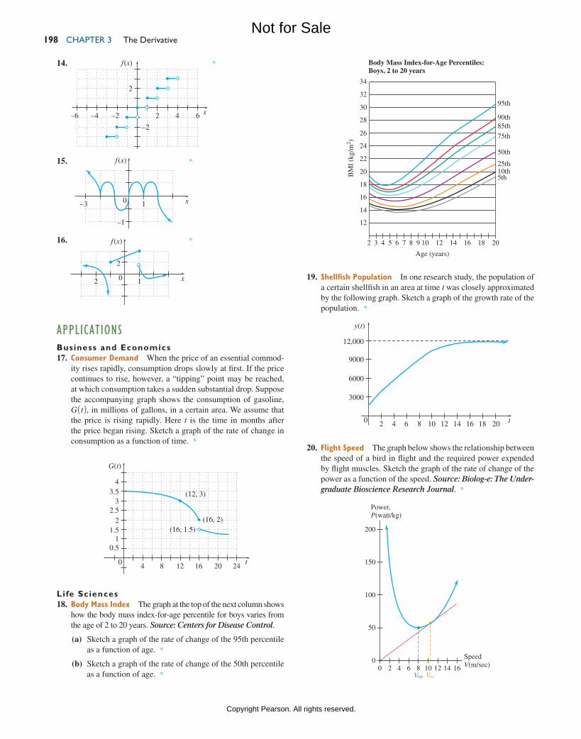
ChAptER 3 the Derivative 198
14.
–2
(x)
2 4 6–6 –2–4 x
2
f *
15. f (x)
x–3
–1
10
*
16. f (x)
x0
2
2 1
*
appLicationsBusiness and Economics 17. consumer Demand When the price of an essential commod-
ity rises rapidly, consumption drops slowly at first. If the price continues to rise, however, a “tipping” point may be reached, at which consumption takes a sudden substantial drop. Suppose the accompanying graph shows the consumption of gasoline, G1t2, in millions of gallons, in a certain area. We assume that the price is rising rapidly. Here t is the time in months after the price began rising. Sketch a graph of the rate of change in consumption as a function of time. *
Life Sciences 18. Body Mass index The graph at the top of the next column shows
how the body mass index-for-age percentile for boys varies from the age of 2 to 20 years. Source: Centers for Disease Control.
(a) Sketch a graph of the rate of change of the 95th percentile as a function of age. *
(b) Sketch a graph of the rate of change of the 50th percentile as a function of age. *
0 4 168 12 20 24t
G(t)
3.5
2.5
4
3
21.5
10.5
(12, 3)
(16, 2)(16, 1.5)
12
14
16
18
20
22
24
26
28
30
32
34
2 3 4 5 6 7 8 9 10 12 14 16 18 20
Age (years)
Body Mass Index-for-Age Percentiles:Boys, 2 to 20 years
BM
I (k
g/m
2 )
95th
90th85th
75th
50th
25th10th5th
19. Shellfish Population In one research study, the population of a certain shellfish in an area at time t was closely approximated by the following graph. Sketch a graph of the growth rate of the population. *
9000
12,000
6000
3000
2 64 108 14 1612 18 20 t
y(t)
0
20. Flight Speed The graph below shows the relationship between the speed of a bird in flight and the required power expended by flight muscles. Sketch the graph of the rate of change of the power as a function of the speed. Source: Biolog-e: The Under-graduate Bioscience Research Journal. *
146 124
150
100
200
50
01610820
SpeedV(m/sec)
Vmp Vmr
Power,P(watt/kg)
M03_LIAL8774_11_AIE_C03_133-208.indd 198 23/06/15 11:33 AM
Not for Sale
Copyright Pearson. All rights reserved.
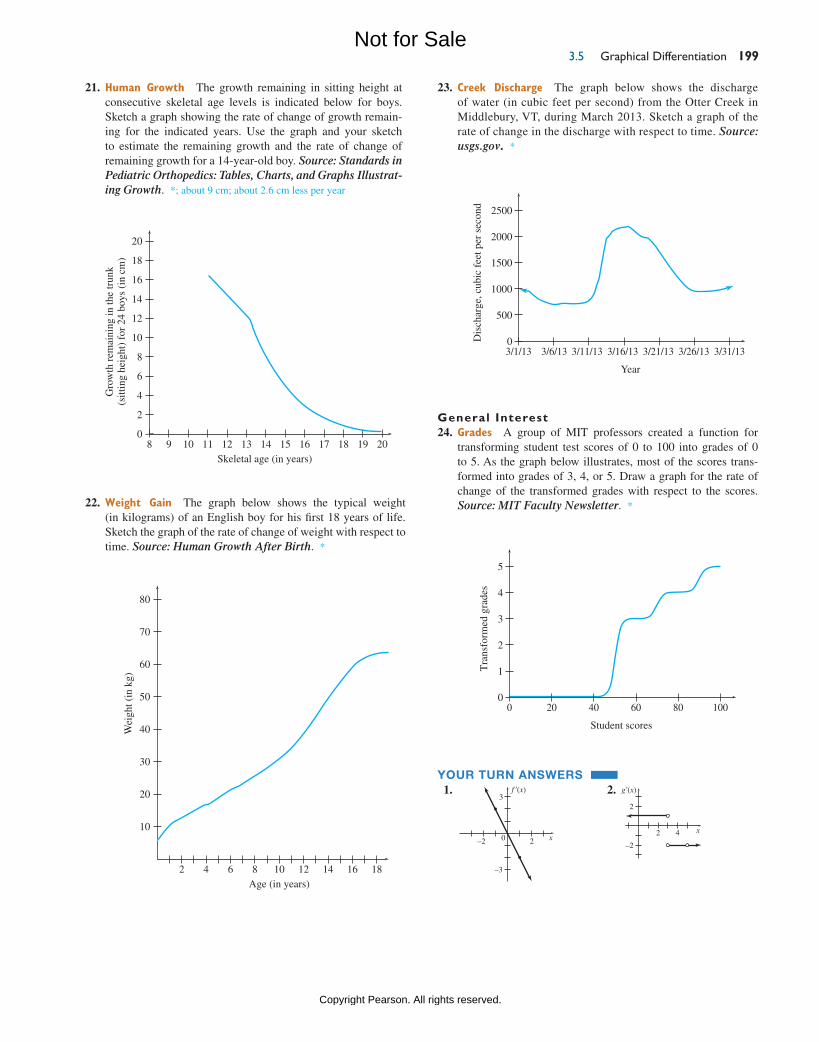
3.5 Graphical Differentiation 199
208 9 10 11 12 13 14 15 16 17 18 19
Gro
wth
rem
aini
ng in
the
trun
k(s
ittin
g he
ight
) fo
r 24
boy
s (i
n cm
)
0
20
18
16
14
12
10
8
6
4
2
Skeletal age (in years)
21. Human Growth The growth remaining in sitting height at consecutive skeletal age levels is indicated below for boys. Sketch a graph showing the rate of change of growth remain-ing for the indicated years. Use the graph and your sketch to estimate the remaining growth and the rate of change of remaining growth for a 14-year-old boy. Source: Standards in Pediatric Orthopedics: Tables, Charts, and Graphs Illustrat-ing Growth. *; about 9 cm; about 2.6 cm less per year
2 4 6 8 10 12 14 16 18
Wei
ght (
in k
g)
10
20
30
40
50
60
70
80
Age (in years)
3/1/13 3/6/13 3/11/13 3/16/13
Year
3/26/13 3/31/133/21/130
500
1000
1500
2000
2500
Dis
char
ge, c
ubic
fee
t per
sec
ond
0 20 40 60
Student scores
80 1000
1
2
3
4
5
Tra
nsfo
rmed
gra
des
General Interest 24. Grades A group of MIT professors created a function for
transforming student test scores of 0 to 100 into grades of 0 to 5. As the graph below illustrates, most of the scores trans-formed into grades of 3, 4, or 5. Draw a graph for the rate of change of the transformed grades with respect to the scores. Source: MIT Faculty Newsletter. *
Your Turn Answers 1.
3
–3
2–2 0 x
f ′(x) 2.
x
g′(x)
2
2 4
–2
22. Weight Gain The graph below shows the typical weight (in kilograms) of an English boy for his first 18 years of life. Sketch the graph of the rate of change of weight with respect to time. Source: Human Growth After Birth. *
23. Creek Discharge The graph below shows the discharge of water (in cubic feet per second) from the Otter Creek in Middlebury, VT, during March 2013. Sketch a graph of the rate of change in the discharge with respect to time. Source: usgs.gov. *
M03_LIAL8774_11_AIE_C03_133-208.indd 199 03/07/15 9:51 AM
Not for Sale
Copyright Pearson. All rights reserved.
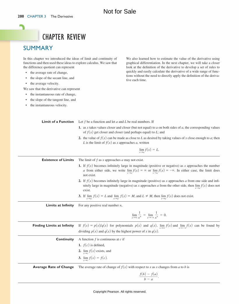
ChAptER 3 the Derivative 200
In this chapter we introduced the ideas of limit and continuity of functions and then used these ideas to explore calculus. We saw that the difference quotient can represent
• theaveragerateofchange,
• theslopeofthesecantline,and
• theaveragevelocity.
We saw that the derivative can represent
• theinstantaneousrateofchange,
• theslopeofthetangentline,and
• theinstantaneousvelocity.
We also learned how to estimate the value of the derivative using graphical differentiation. In the next chapter, we will take a closer look at the definition of the derivative to develop a set of rules to quickly and easily calculate the derivative of a wide range of func-tions without the need to directly apply the definition of the deriva-tive each time.
SuMMARy
3 cHapter review
Limit of a Function Let ƒ be a function and let a and L be real numbers. If
1. as x takes values closer and closer (but not equal) to a on both sides of a, the corresponding values of ƒ1x2 get closer and closer (and perhaps equal) to L; and
2. the value of ƒ1x2 can be made as close to L as desired by taking values of x close enough to a; then L is the limit of ƒ1x2 as x approaches a, written
limxSa
ƒ1x2 = L.
Existence of Limits The limit of ƒ as x approaches a may not exist.
1. If ƒ1x2 becomes infinitely large in magnitude (positive or negative) as x approaches the number a from either side, we write lim
xSa ƒ1x2 = ∞ or lim
xSa ƒ1x2 = -∞. In either case, the limit does
not exist.
2. If ƒ1x2 becomes infinitely large in magnitude (positive) as x approaches a from one side and infi-nitely large in magnitude (negative) as x approaches a from the other side, then lim
xSa ƒ1x2 does not
exist.
3. If limxSa- ƒ1x2 = L and lim
xSa+ ƒ1x2 = M, and L Z M, then limxSa
ƒ1x2 does not exist.
Limits at Infinity For any positive real number n,
limxS∞
1
xn = limxS-∞
1
xn = 0.
Finding Limits at Infinity If ƒ1x2 = p1x2/q1x2 for polynomials p1x2 and q1x2, limxS∞
ƒ1x2 and limxS-∞
ƒ1x2 can be found by
dividing p1x2 and q1x2 by the highest power of x in q1x2.
Continuity A function ƒ is continuous at c if
1. ƒ1c2 is defined,
2. limxSc
ƒ1x2 exists, and
3. limxSc
ƒ1x2 = ƒ1c2.
Average Rate of Change The average rate of change of ƒ1x2 with respect to x as x changes from a to b is
ƒ1b2 - ƒ1a2b - a
.
M03_LIAL8774_11_AIE_C03_133-208.indd 200 23/06/15 11:34 AM
Not for Sale
Copyright Pearson. All rights reserved.
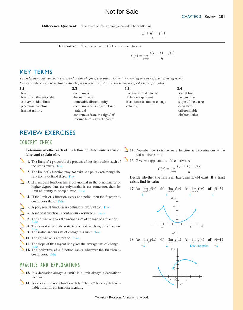
ChAptER 3 Review 201
Difference Quotient The average rate of change can also be written as
ƒ1x + h2 - ƒ1x2h
.
Derivative The derivative of ƒ1x2 with respect to x is
ƒ′1x2 = limhS0
ƒ1x + h2 - ƒ1x2
h .
KEy tERMS
3.1limitlimit from the left/rightone-/two-sided limitpiecewise functionlimit at infinity
3.2continuousdiscontinuousremovable discontinuitycontinuous on an open/closed intervalcontinuous from the right/leftIntermediate Value Theorem
3.3average rate of changedifference quotientinstantaneous rate of changevelocity
3.4secant linetangent lineslope of the curvederivativedifferentiabledifferentiation
To understand the concepts presented in this chapter, you should know the meaning and use of the following terms. For easy reference, the section in the chapter where a word (or expression) was first used is provided.
Determine whether each of the following statements is true or false, and explain why.
1. The limit of a product is the product of the limits when each of the limits exists. True
2. The limit of a function may not exist at a point even though the function is defined there. True
3. If a rational function has a polynomial in the denominator of higher degree than the polynomial in the numerator, then the limit at infinity must equal zero. True
4. If the limit of a function exists at a point, then the function is continuous there. False
5. A polynomial function is continuous everywhere. True
6. A rational function is continuous everywhere. False
7. The derivative gives the average rate of change of a function. False 8. The derivative gives the instantaneous rate of change of a function.
9. The instantaneous rate of change is a limit. True
10. The derivative is a function. True
11. The slope of the tangent line gives the average rate of change. False 12. The derivative of a function exists wherever the function is
continuous. False
REvIEW ExERCISES
concept cHeck 15. Describe how to tell when a function is discontinuous at the
real number x = a.
16. Give two applications of the derivative
ƒ′1x2 = limhS0
ƒ1x + h2 - ƒ1x2
h .
Decide whether the limits in Exercises 17–34 exist. If a limit exists, find its value.
17. (a) limxS-3 -
ƒ1x2 (b) limxS-3+
ƒ1x2 (c) limxS-3
ƒ1x2 (d) ƒ1-32 4 4 4 4
–2
f(x)
3–3 x
4
18. (a) limxS-1-
g1x2 (b) limxS-1+
g1x2 (c) limxS-1
g1x2 (d) g1-12 -2 2 Does not exist -2
–2
g(x)
2–2 x
2
0
practice anD expLorations 13. Is a derivative always a limit? Is a limit always a derivative?
Explain.
14. Is every continuous function differentiable? Is every differen-tiable function continuous? Explain.
True
M03_LIAL8774_11_AIE_C03_133-208.indd 201 23/06/15 11:34 AM
Not for Sale
Copyright Pearson. All rights reserved.
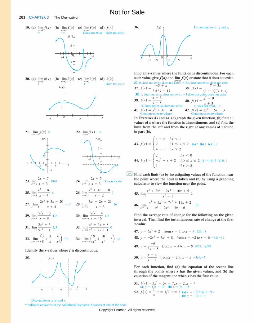
Chapter 3 the Derivative 202
19. (a) limxS4-
ƒ1x2 (b) limxS4+
ƒ1x2 (c) limxS4
ƒ1x2 (d) ƒ142 ∞ -∞ Does not exist Does not exist
f(x)
–4 4 x
3
0
–3
20. (a) limxS2-
h1x2 (b) limxS2+
h1x2 (c) limxS2
h1x2 (d) h122 1 1 1 Does not exist
h(x)
–2 2 x
1
0
21. limxS-∞
g1x2 ∞
–2
g(x)
2–2 x
2
0
22. limxS∞
ƒ1x2 -3
f(x)
4–4 x
3
–3
0
23. limxS6
2x + 7
x + 3 19/9 24. lim
xS-3 2x + 5
x + 3 Does not exist
25. limxS4
x2 - 16
x - 4 8 26. lim
xS2 x2 + 3x - 10
x - 2 7
27. limxS-4
2x2 + 3x - 20
x + 4 -13 28. lim
xS3 3x2 - 2x - 21
x - 3 16
29. limxS9
2x - 3
x - 9 1/6 30. lim
xS16 2x - 4
x - 16 1/8
31. limxS∞
2x2 + 5
5x2 - 1 2/5 32. lim
xS∞ x2 + 6x + 8
x3 + 2x + 1 0
33. limxS-∞
a38
+3x
-6
x2b 3/8 34. limxS-∞
a 9
x4 +10
x2 - 6b -6
Identify the x-values where ƒ is discontinuous.
35. f(x)
x0x1 x2 x3 x4
Discontinuous at x2 and x4
* indicates answer is in the Additional Instructor Answers at end of the book.
37. 0, does not exist, does not exist; -1/3, does not exist, does not exist
38. 1, does not exist, does not exist; -3 does not exist, does not exist
36. f(x)
0x x x xx1 2 3 4
Discontinuous at x1 and x4
Find all x-values where the function is discontinuous. For each such value, give ƒ 1a 2 and lim
xS a ƒ 1x 2 or state that it does not exist.
37. ƒ1x2 =-5 + x
3x13x + 12 38. ƒ1x2 =7 - 3x
11 - x213 + x2
39. ƒ1x2 =x - 6
x + 5-5, does not exist, does not exist
40. ƒ1x2 =x2 - 9
x + 3-3, does not exist, -6
41. ƒ1x2 = x2 + 3x - 4 Continuous everywhere
42. ƒ1x2 = 2x2 - 5x - 3 Continuous everywhere
In Exercises 43 and 44, (a) graph the given function, (b) find all values of x where the function is discontinuous, and (c) find the limit from the left and from the right at any values of x found in part (b).
43. ƒ1x2 = c 1 - x
2
4 - x
if x 6 1
if 1 … x … 2
if x 7 2
(a) * (b) 1 (c) 0, 2
44. ƒ1x2 = c 2
-x2 + x + 2
1
if x 6 0
if 0 … x … 2
if x 7 2
(a) * (b) 2 (c) 0, 1
Find each limit (a) by investigating values of the function near the point where the limit is taken and (b) by using a graphing calculator to view the function near the point.
45. limxS1
x4 + 2x3 + 2x2 - 10x + 5
x2 - 1 2
46. limxS-2
x4 + 3x3 + 7x2 + 11x + 2
x3 + 2x2 - 3x - 6 -13
Find the average rate of change for the following on the given interval. Then find the instantaneous rate of change at the first x-value.
47. y = 6x3 + 2 from x = 1 to x = 4 126; 18
48. y = -2x3 - 3x2 + 8 from x = -2 to x = 6 -68; -12
49. y =-6
3x - 5 from x = 4 to x = 9 9/77; 18/49
50. y =x + 4
x - 1 from x = 2 to x = 5 -5/4; -5
For each function, find (a) the equation of the secant line through the points where x has the given values, and (b) the equation of the tangent line when x has the first value.
51. ƒ1x2 = 3x2 - 5x + 7; x = 2, x = 4 (a) y = 13x - 17 (b) y = 7x - 5
52. ƒ 1x2 =1x
; x = 1/2, x = 3 (a) y = -12/32x + 7/3 (b) y = -4x + 4
M03_LIAL8774_11_AIE_C03_133-208.indd 202 03/07/15 9:52 AM
Not for Sale
Copyright Pearson. All rights reserved.
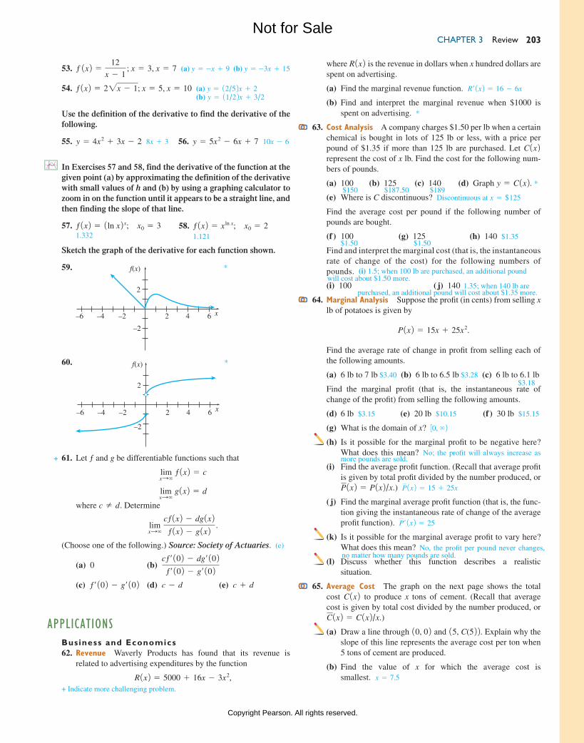
CHAPTER 3 Review 203
53. ƒ 1x2 =12
x - 1 ; x = 3, x = 7 (a) y = -x + 9 (b) y = -3x + 15
54. ƒ1x2 = 22x - 1; x = 5, x = 10 (a) y = 12/52x + 2 (b) y = 11/22x + 3/2
Use the definition of the derivative to find the derivative of the following.
55. y = 4x2 + 3x - 2 8x + 3 56. y = 5x2 - 6x + 7 10x - 6
In Exercises 57 and 58, find the derivative of the function at the given point (a) by approximating the definition of the derivative with small values of h and (b) by using a graphing calculator to zoom in on the function until it appears to be a straight line, and then finding the slope of that line.
57. ƒ1x2 = 1ln x2x; x0 = 3 1.332
58. ƒ1x2 = x ln x; x0 = 2 1.121
Sketch the graph of the derivative for each function shown.
59.
–2
f(x)
2 4–4 6–6 –2 x
2
*
60.
–2
f(x)
2 4 6–6 –2–4 x
2
*
61. Let ƒ and g be differentiable functions such that
limxS∞
ƒ1x2 = c
limxS∞
g1x2 = d
where c Z d. Determine
limxS∞
cƒ1x2 - dg1x2ƒ1x2 - g1x2 .
(Choose one of the following.) Source: Society of Actuaries. (e)
(a) 0 (b) cƒ′102 - dg′102ƒ′102 - g′102
(c) ƒ′102 - g′102 (d) c - d (e) c + d
+
where R1x2 is the revenue in dollars when x hundred dollars are spent on advertising.
(a) Find the marginal revenue function. R′1x2 = 16 - 6x
(b) Find and interpret the marginal revenue when $1000 is spent on advertising. *
63. Cost Analysis A company charges $1.50 per lb when a certain chemical is bought in lots of 125 lb or less, with a price per pound of $1.35 if more than 125 lb are purchased. Let C1x2 represent the cost of x lb. Find the cost for the following num-bers of pounds.
(a) 100 (b) 125 (c) 140 (d) Graph y = C1x2. *$150 $187.50 $189
(e) Where is C discontinuous? Discontinuous at x = +125
Find the average cost per pound if the following number of pounds are bought.
(f ) 100 (g) 125 (h) 140 $1.35$1.50 $1.50
Find and interpret the marginal cost (that is, the instantaneous rate of change of the cost) for the following numbers of pounds.
(i) 100 ( j) 140
64. Marginal Analysis Suppose the profit (in cents) from selling x lb of potatoes is given by
P1x2 = 15x + 25x2.
Find the average rate of change in profit from selling each of the following amounts.
(a) 6 lb to 7 lb $3.40 (b) 6 lb to 6.5 lb $3.28 (c) 6 lb to 6.1 lb
Find the marginal profit (that is, the instantaneous rate of change of the profit) from selling the following amounts.
(d) 6 lb $3.15 (e) 20 lb $10.15 (f ) 30 lb $15.15
(g) What is the domain of x? 30, ∞2 (h) Is it possible for the marginal profit to be negative here?
What does this mean? No; the profit will always increase as more pounds are sold.
(i) Find the average profit function. (Recall that average profit is given by total profit divided by the number produced, or P1x2 = P1x2/x.) P1x2 = 15 + 25x
( j) Find the marginal average profit function (that is, the func-tion giving the instantaneous rate of change of the average profit function). P′1x2 = 25
(k) Is it possible for the marginal average profit to vary here? What does this mean?
(l) Discuss whether this function describes a realistic situation.
65. Average Cost The graph on the next page shows the total cost C1x2 to produce x tons of cement. (Recall that average cost is given by total cost divided by the number produced, or C1x2 = C1x2/x.)
(a) Draw a line through 10, 02 and 15, C(522. Explain why the slope of this line represents the average cost per ton when 5 tons of cement are produced.
(b) Find the value of x for which the average cost is smallest. x = 7.5
ApplicAtionsBusiness and Economics 62. Revenue Waverly Products has found that its revenue is
related to advertising expenditures by the function
R1x2 = 5000 + 16x - 3x2,+ Indicate more challenging problem.
(i) 1.5; when 100 lb are purchased, an additional pound
No, the profit per pound never changes, no matter how many pounds are sold.
1.35; when 140 lb are
$3.18
will cost about $1.50 more.
purchased, an additional pound will cost about $1.35 more.
M03_LIAL8774_11_AIE_C03_133-208.indd 203 03/07/15 9:54 AM
Not for Sale
Copyright Pearson. All rights reserved.
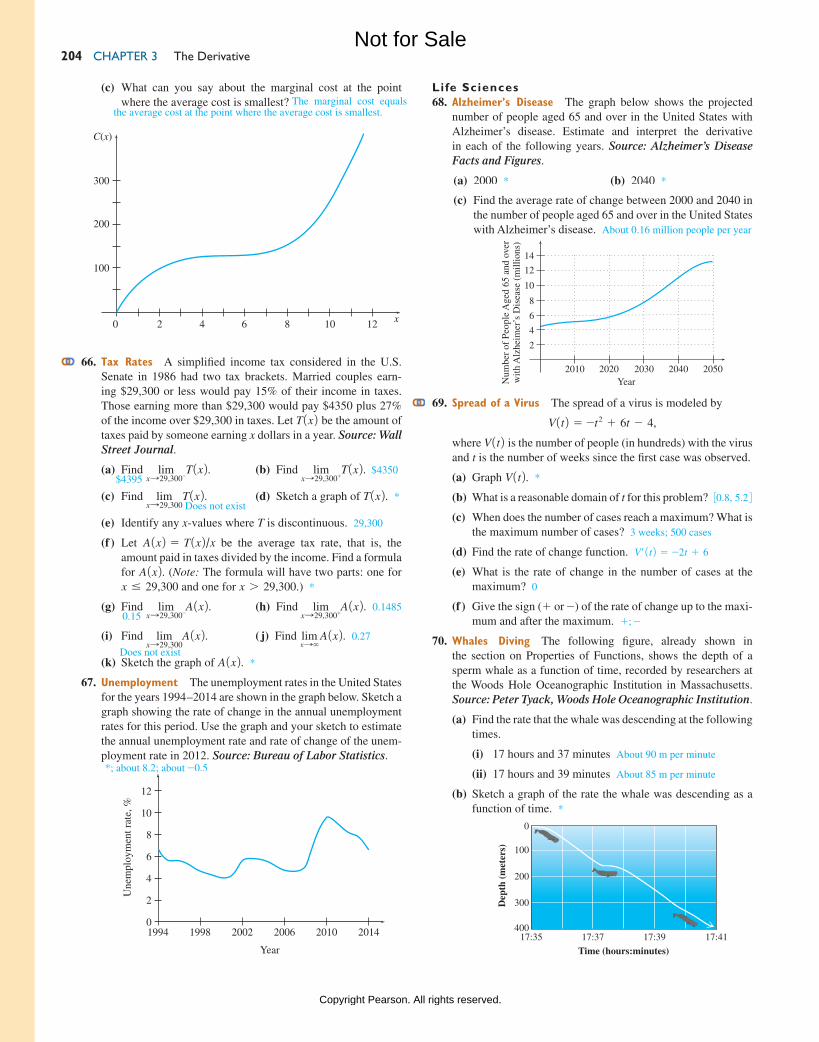
ChAptER 3 the Derivative 204
(c) What can you say about the marginal cost at the point where the average cost is smallest?
Life Sciences 68. alzheimer’s Disease The graph below shows the projected
number of people aged 65 and over in the United States with Alzheimer’s disease. Estimate and interpret the derivative in each of the following years. Source: Alzheimer’s Disease Facts and Figures.
(a) 2000 * (b) 2040 *
(c) Find the average rate of change between 2000 and 2040 in the number of people aged 65 and over in the United States with Alzheimer’s disease. About 0.16 million people per year
2010 2020 2030 2040 2050
4
8
12
14
2
6
10
Num
ber
of P
eopl
e A
ged
65 a
nd o
ver
with
Alz
heim
er’s
Dis
ease
(m
illio
ns)
Year
69. Spread of a Virus The spread of a virus is modeled by
V1t2 = -t2 + 6t - 4,
where V1t2 is the number of people (in hundreds) with the virus and t is the number of weeks since the first case was observed.
(a) Graph V1t2. *
(b) What is a reasonable domain of t for this problem? 30.8, 5.24(c) When does the number of cases reach a maximum? What is
the maximum number of cases? 3 weeks; 500 cases
(d) Find the rate of change function. V′1t2 = -2t + 6
(e) What is the rate of change in the number of cases at the maximum? 0
(f ) Give the sign (+ or -) of the rate of change up to the maxi-mum and after the maximum. + ; -
70. Whales Diving The following figure, already shown in the section on Properties of Functions, shows the depth of a sperm whale as a function of time, recorded by researchers at the Woods Hole Oceanographic Institution in Massachusetts. Source: Peter Tyack, Woods Hole Oceanographic Institution.
(a) Find the rate that the whale was descending at the following times.
(i) 17 hours and 37 minutes About 90 m per minute
(ii) 17 hours and 39 minutes About 85 m per minute
(b) Sketch a graph of the rate the whale was descending as a function of time. *
17:35 17:37 17:39 17:41400
300
200
100
0
Dep
th (
met
ers)
Time (hours:minutes)
420 6 8 10 12
C(x)
x
200
300
100
The marginal cost equals
66. tax Rates A simplified income tax considered in the U.S. Senate in 1986 had two tax brackets. Married couples earn-ing $29,300 or less would pay 15% of their income in taxes. Those earning more than $29,300 would pay $4350 plus 27% of the income over $29,300 in taxes. Let T1x2 be the amount of taxes paid by someone earning x dollars in a year. Source: Wall Street Journal.
(a) Find limxS29,300-
T1x2. (b) Find limxS29,300+
T1x2. $4350$4395
(c) Find limxS29,300
T1x2. (d) Sketch a graph of T1x2. *Does not exist
(e) Identify any x-values where T is discontinuous. 29,300
(f ) Let A1x2 = T1x2/x be the average tax rate, that is, the amount paid in taxes divided by the income. Find a formula for A1x2. (Note: The formula will have two parts: one for x … 29,300 and one for x 7 29,300.) *
(g) Find limxS29,300-
A1x2. (h) Find limxS29,300+
A1x2. 0.14850.15
(i) Find limxS29,300
A1x2. ( j) Find limxS∞
A1x2. 0.27
Does not exist(k) Sketch the graph of A1x2. *
67. unemployment The unemployment rates in the United States for the years 1994–2014 are shown in the graph below. Sketch a graph showing the rate of change in the annual unemployment rates for this period. Use the graph and your sketch to estimate the annual unemployment rate and rate of change of the unem-ployment rate in 2012. Source: Bureau of Labor Statistics.*; about 8.2; about -0.5
1994 1998 2002 2006
Year
2010 20140
2
4
6
8
10
12
Une
mpl
oym
ent r
ate,
%the average cost at the point where the average cost is smallest.
M03_LIAL8774_11_AIE_C03_133-208.indd 204 23/06/15 11:34 AM
Not for Sale
Copyright Pearson. All rights reserved.

CHAPTER 3 Review 205
71. Body Mass Index The following graph shows how the body mass index-for-age percentile for girls varies from the age of 2 to 20 years. Source: Centers for Disease Control.
(a) Sketch a graph of the rate of change of the 95th percentile as a function of age.
(b) Sketch a graph of the rate of change of the 50th percentile as a function of age.
Body Mass Index-for-Age Percentiles:Girls, 2 to 20 years
12
14
16
18
20
22
24
26
28
30
32
34
2 3 4 5 6 7 8 9 10 12 14 16 18 20
Age (years)
BM
I (k
g/m
2 )
95th
97th
90th
85th
75th
50th
25th10th3rd
72. Human Growth The growth remaining in sitting height for girls at consecutive skeletal age levels is indicated on the graph in the next column. Sketch a graph showing the rate of change of growth remaining for the indicated years. Use the graph and your sketch to estimate the remaining growth and the rate of change of remaining growth for a 10-year-old girl. Source: Standards in Pediatric Orthopedics: Tables, Charts, and Graphs Illustrating Growth.
208 9 10 11 12 13 14 15 16 17 18 19
Gro
wth
rem
aini
ng in
the
trun
k(s
ittin
g he
ight
in c
m)
0
20
18
16
14
12
10
8
6
4
2
Skeletal age (in years)
Physical Sciences 73. Temperature Suppose a gram of ice is at a temperature of
-100°C. The graph shows the temperature of the ice as increas-ing numbers of calories of heat are applied. It takes 80 calories to melt one gram of ice at 0°C into water, and 540 calories to boil one gram of water at 100°C into steam.
(a) Where is this graph discontinuous? Nowhere
(b) Where is this graph not differentiable? 50, 130, 230, 770
(c) Sketch the graph of the derivative.
200
–100500
50
T (degrees C)
0 Q (calories)
71. (a)
206 10
1
–1
–2
2
Rat
e of
cha
nge
of B
MI
Age (years)
(b)
206 10
1
–1
–2
2
Rat
e of
cha
nge
of B
m2
Age (years)
72. The remaining growth is about 14 cm and the rate of change is about -2.75 cm per year.
73. (c)
M03_LIAL8774_11_AIE_C03_133-208.indd 205 03/07/15 9:57 AM
Not for Sale
Copyright Pearson. All rights reserved.
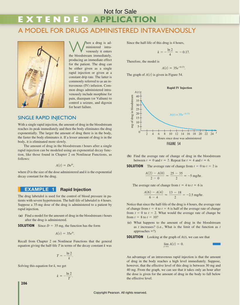
206 PB
A MoDEL foR DRuGS ADMInIStERED IntRAvEnouSLy
When a drug is ad-ministered intra-venously it enters
the bloodstream immediately, producing an immediate effect for the patient. The drug can be either given as a single rapid injection or given at a constant drip rate. The latter is commonly referred to as an in-travenous (IV) infusion. Com-mon drugs administered intra-venously include morphine for pain, diazepam (or Valium) to control a seizure, and digoxin for heart failure.
SInGLE RApID InjECtIonWith a single rapid injection, the amount of drug in the bloodstream reaches its peak immediately and then the body eliminates the drug exponentially. The larger the amount of drug there is in the body, the faster the body eliminates it. If a lesser amount of drug is in the body, it is eliminated more slowly.
The amount of drug in the bloodstream t hours after a single rapid injection can be modeled using an exponential decay func-tion, like those found in Chapter 2 on Nonlinear Functions, as follows:
A1t2 = Dekt,
where D is the size of the dose administered and k is the exponential decay constant for the drug.
E x t E n d E d APPLICATIon
ExampLE 1 Rapid InjectionThe drug labetalol is used for the control of blood pressure in pa-tients with severe hypertension. The half-life of labetalol is 4 hours. Suppose a 35-mg dose of the drug is administered to a patient by rapid injection.
(a) Find a model for the amount of drug in the bloodstream t hours after the drug is administered.
Solution Since D = 35 mg, the function has the form
A1t2 = 35ekt.
Recall from Chapter 2 on Nonlinear Functions that the general equation giving the half-life T in terms of the decay constant k was
T = - ln 2
k .
Solving this equation for k, we get
k = - ln 2
T .
Since the half-life of this drug is 4 hours,
k = - ln 2
4 ≈ - 0.17.
Therefore, the model is
A1t2 = 35e-0.17t.
The graph of A1t2 is given in Figure 54.
Figure 54
510
1520253035
40
mg
of d
rug
in b
lood
stre
am
Rapid IV Injection
Hours since dose was administered
2 4 6 8 10 12 14 16 18 20 22 240
A (t )
t
A (t ) = 35e–0.17t
(b) Find the average rate of change of drug in the bloodstream between t = 0 and t = 2. Repeat for t = 4 and t = 6.
Solution The average rate of change from t = 0 to t = 2 is
A122 - A1022 - 0
≈25 - 35
2= -5 mg/hr.
The average rate of change from t = 4 to t = 6 is
A162 - A1426 - 4
≈13 - 18
2= -2.5 mg/hr.
Notice that since the half-life of the drug is 4 hours, the average rate of change from t = 4 to t = 6 is half of the average rate of change from t = 0 to t = 2. What would the average rate of change be from t = 8 to t = 10?
(c) What happens to the amount of drug in the bloodstream as t increases? (i.e., What is the limit of the function as t approaches ∞?)
Solution Looking at the graph of A(t), we can see that
limtS∞
A1t2 = 0.
An advantage of an intravenous rapid injection is that the amount of drug in the body reaches a high level immediately. Suppose, however, that the effective level of this drug is between 30 mg and 40 mg. From the graph, we can see that it takes only an hour after the dose is given for the amount of drug in the body to fall below the effective level.
M03_LIAL8774_11_AIE_C03_133-208.indd 206 23/06/15 11:35 AM
Not for Sale
Copyright Pearson. All rights reserved.
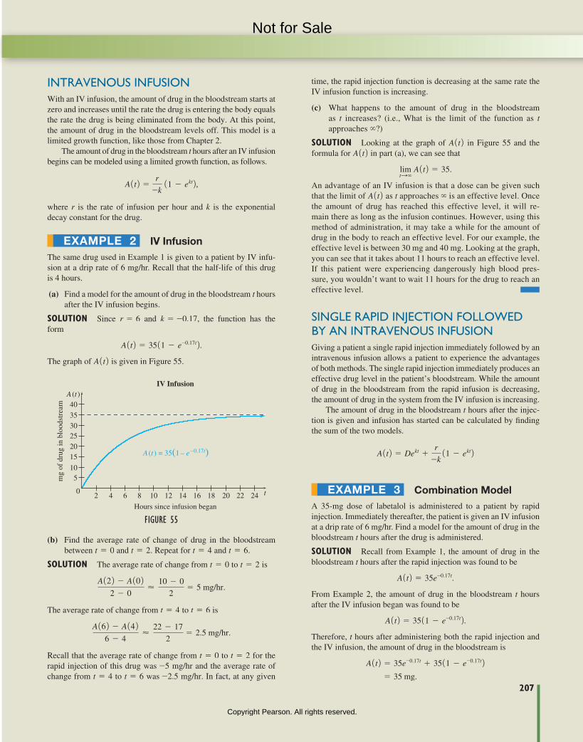
PB 207
IntRAvEnouS InfuSIonWith an IV infusion, the amount of drug in the bloodstream starts at zero and increases until the rate the drug is entering the body equals the rate the drug is being eliminated from the body. At this point, the amount of drug in the bloodstream levels off. This model is a limited growth function, like those from Chapter 2.
The amount of drug in the bloodstream t hours after an IV infusion begins can be modeled using a limited growth function, as follows.
A1t2 =r
-k 11 - ekt2,
where r is the rate of infusion per hour and k is the exponential decay constant for the drug.
ExampLE 2 IV InfusionThe same drug used in Example 1 is given to a patient by IV infu-sion at a drip rate of 6 mg/hr. Recall that the half-life of this drug is 4 hours.
(a) Find a model for the amount of drug in the bloodstream t hours after the IV infusion begins.
Solution Since r = 6 and k = -0.17, the function has the form
A1t2 = 3511 - e-0.17t2.The graph of A1t2 is given in Figure 55.
Figure 55
510
1520253035
40
mg
of d
rug
in b
lood
stre
am
IV Infusion
Hours since infusion began
2 4 6 8 10 12 14 16 18 20 22 240
A (t )
t
A (t ) = 35(1 – e–0.17t)
(b) Find the average rate of change of drug in the bloodstream between t = 0 and t = 2. Repeat for t = 4 and t = 6.
Solution The average rate of change from t = 0 to t = 2 is
A122 - A1022 - 0
≈10 - 0
2= 5 mg/hr.
The average rate of change from t = 4 to t = 6 is
A162 - A1426 - 4
≈22 - 17
2= 2.5 mg/hr.
Recall that the average rate of change from t = 0 to t = 2 for the rapid injection of this drug was -5 mg/hr and the average rate of change from t = 4 to t = 6 was -2.5 mg/hr. In fact, at any given
time, the rapid injection function is decreasing at the same rate the IV infusion function is increasing.
(c) What happens to the amount of drug in the bloodstream as t increases? (i.e., What is the limit of the function as t approaches ∞?)
Solution Looking at the graph of A1t2 in Figure 55 and the formula for A1t2 in part (a), we can see that
limtS∞
A1t2 = 35.
An advantage of an IV infusion is that a dose can be given such that the limit of A1t2 as t approaches ∞ is an effective level. Once the amount of drug has reached this effective level, it will re-main there as long as the infusion continues. However, using this method of administration, it may take a while for the amount of drug in the body to reach an effective level. For our example, the effective level is between 30 mg and 40 mg. Looking at the graph, you can see that it takes about 11 hours to reach an effective level. If this patient were experiencing dangerously high blood pres-sure, you wouldn’t want to wait 11 hours for the drug to reach an effective level.
SInGLE RApID InjECtIon foLLoWED by An IntRAvEnouS InfuSIonGiving a patient a single rapid injection immediately followed by an intravenous infusion allows a patient to experience the advantages of both methods. The single rapid injection immediately produces an effective drug level in the patient’s bloodstream. While the amount of drug in the bloodstream from the rapid infusion is decreasing, the amount of drug in the system from the IV infusion is increasing.
The amount of drug in the bloodstream t hours after the injec-tion is given and infusion has started can be calculated by finding the sum of the two models.
A1t2 = Dekt +r
-k 11 - ekt2
ExampLE 3 Combination modelA 35-mg dose of labetalol is administered to a patient by rapid injection. Immediately thereafter, the patient is given an IV infusion at a drip rate of 6 mg/hr. Find a model for the amount of drug in the bloodstream t hours after the drug is administered.
Solution Recall from Example 1, the amount of drug in the bloodstream t hours after the rapid injection was found to be
A1t2 = 35e-0.17t.
From Example 2, the amount of drug in the bloodstream t hours after the IV infusion began was found to be
A1t2 = 3511 - e-0.17t2.Therefore, t hours after administering both the rapid injection and the IV infusion, the amount of drug in the bloodstream is
A1t2 = 35e-0.17t + 3511 - e-0.17t2 = 35 mg.
M03_LIAL8774_11_AIE_C03_133-208.indd 207 23/06/15 11:35 AM
Not for Sale
Copyright Pearson. All rights reserved.
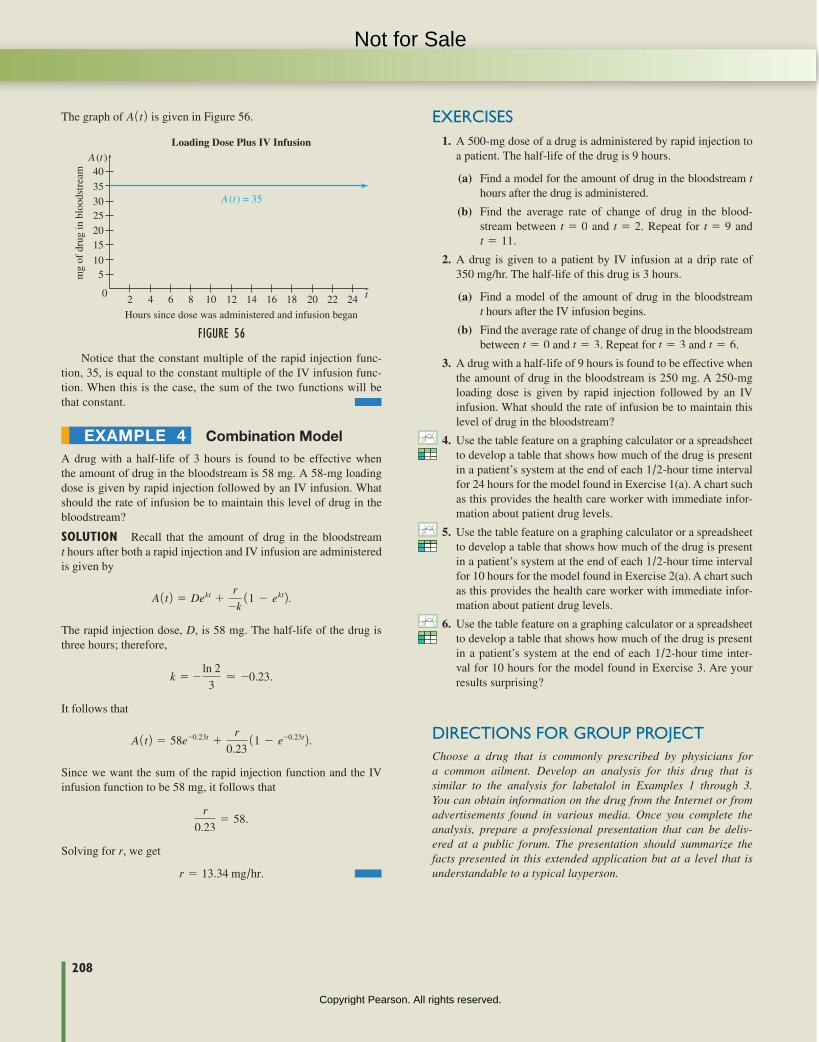
208 PB
The graph of A1t2 is given in Figure 56.
Figure 56
510
1520253035
40
mg
of d
rug
in b
lood
stre
am
Loading Dose Plus IV Infusion
Hours since dose was administered and infusion began
2 4 6 8 10 12 14 16 18 20 22 240
A (t )
t
A (t ) = 35
Notice that the constant multiple of the rapid injection func-tion, 35, is equal to the constant multiple of the IV infusion func-tion. When this is the case, the sum of the two functions will be that constant.
ExampLE 4 Combination modelA drug with a half-life of 3 hours is found to be effective when the amount of drug in the bloodstream is 58 mg. A 58-mg loading dose is given by rapid injection followed by an IV infusion. What should the rate of infusion be to maintain this level of drug in the bloodstream?
Solution Recall that the amount of drug in the bloodstream t hours after both a rapid injection and IV infusion are administered is given by
A1t2 = Dekt +r
-k 11 - ekt2.
The rapid injection dose, D, is 58 mg. The half-life of the drug is three hours; therefore,
k = - ln 2
3≈ -0.23.
It follows that
A1t2 = 58e-0.23t +r
0.23 11 - e-0.23t2.
Since we want the sum of the rapid injection function and the IV infusion function to be 58 mg, it follows that
r
0.23= 58.
Solving for r, we get
r = 13.34 mg/hr.
ExERCISES 1. A 500-mg dose of a drug is administered by rapid injection to
a patient. The half-life of the drug is 9 hours.
(a) Find a model for the amount of drug in the bloodstream t hours after the drug is administered.
(b) Find the average rate of change of drug in the blood-stream between t = 0 and t = 2. Repeat for t = 9 and t = 11.
2. A drug is given to a patient by IV infusion at a drip rate of 350 mg/hr. The half-life of this drug is 3 hours.
(a) Find a model of the amount of drug in the bloodstream t hours after the IV infusion begins.
(b) Find the average rate of change of drug in the bloodstream between t = 0 and t = 3. Repeat for t = 3 and t = 6.
3. A drug with a half-life of 9 hours is found to be effective when the amount of drug in the bloodstream is 250 mg. A 250-mg loading dose is given by rapid injection followed by an IV infusion. What should the rate of infusion be to maintain this level of drug in the bloodstream?
4. Use the table feature on a graphing calculator or a spreadsheet to develop a table that shows how much of the drug is present in a patient’s system at the end of each 1/2-hour time interval for 24 hours for the model found in Exercise 1(a). A chart such as this provides the health care worker with immediate infor-mation about patient drug levels.
5. Use the table feature on a graphing calculator or a spreadsheet to develop a table that shows how much of the drug is present in a patient’s system at the end of each 1/2-hour time interval for 10 hours for the model found in Exercise 2(a). A chart such as this provides the health care worker with immediate infor-mation about patient drug levels.
6. Use the table feature on a graphing calculator or a spreadsheet to develop a table that shows how much of the drug is present in a patient’s system at the end of each 1/2-hour time inter-val for 10 hours for the model found in Exercise 3. Are your results surprising?
DIRECtIonS foR GRoup pRojECtChoose a drug that is commonly prescribed by physicians for a common ailment. Develop an analysis for this drug that is similar to the analysis for labetalol in Examples 1 through 3. You can obtain information on the drug from the Internet or from advertisements found in various media. Once you complete the analysis, prepare a professional presentation that can be deliv-ered at a public forum. The presentation should summarize the facts presented in this extended application but at a level that is understandable to a typical layperson.
M03_LIAL8774_11_AIE_C03_133-208.indd 208 23/06/15 11:35 AM
Not for Sale
Copyright Pearson. All rights reserved.