The Delivery Option in Credit Default Swaps

R. Jankowitsch†, R. Pullirsch‡, T. Veza††

Working paper

First version: May 18, 2006This version: October 18, 2006

Abstract

Under standard assumptions the reduced-form credit risk model is not capable of ac-curately pricing the two fundamental credit risk instruments – bonds and credit defaultswaps (CDS) – simultaneously. Using a data set of euro-denominated corporate bonds andCDS our paper quantifies this mispricing by calibrating such a model to the bond data andsubsequently using it to price CDS, resulting in model CDS spreads up to 50% lower onaverage than observed in the market. An extended model is presented which includes thedelivery option implicit in CDS contracts emerging since a basket of bonds is deliverable indefault. By using a constant recovery rate standard models assume equal recoveries for allbonds and hence zero value for the delivery option. Contradicting this common assumption,case studies of Chapter 11 filings presented in the paper show that corporate bonds do not

trade at equal levels following default. Our extension models the implied expected recov-ery rate of the cheapest-to-deliver bond and, applied to the data, it largely eliminates themispricing. The calibrated recovery values lie between 8% and 47% for different obligors,exhibiting strong variation among rating classes and industries. A cross-sectional analysisreveals that the implied recovery parameter depends on proxies for the delivery option,primarily the number of available bonds and the bond pricing errors. No evidence is foundfor the influence of liquidity proxies.

JEL classification: C13, G12, G13, G15

Keywords: credit risk, default, corporate bond, credit default swap, reduced-form model,recovery rate, delivery option

†Corresponding author. Vienna University of Economics and Business Administration,rainer.jankowitsch@wu-wien.ac.at

‡Bank Austria–Creditanstalt, rainer.pullirsch@ba-ca.com††Vienna University of Economics and Business Administration, tanja.veza@wu-wien.ac.at

1 Introduction

The pace at which the credit derivatives market has been growing since its inceptionabout ten years ago topped all projections1, increasingly calling for the development ofmore and more accurate pricing tools for these products since market reality often revealsthat the assumptions underlying the prevalent models are inadequate and misleading.

The instrument this paper focuses on is a credit default swap (CDS). This is a bilateralcontract aimed at transferring the credit risk of a (corporate or sovereign) borrower fromone market participant (the protection buyer) to another (the protection seller). The CDSbuyer pays a periodical premium for the assurance that the CDS seller will compensatehim for the loss in case the borrower defaults during the term of the contract. If so,the protection seller pays the notional amount of the contract to the protection buyer ascompensation for the loss incurred. The latter, in turn, must deliver obligations (usuallybonds) of the defaulted borrower with total principal equal to the notional amount of theCDS contract.

Since the CDS is a derivative instrument based on defaultable debt as the underlyingasset, it is natural to enquire about the relation between the prices of credit risk in thebond and derivatives markets charged for resp. to a particular borrower. Such a relationis of crucial importance for pricing and hedging credit exposures. Duffie [8] showsthat it is only under highly restrictive and simplifying assumptions that the intuitiveequality between the premium on a CDS and the yield spread of a bond over its risk-freecounterpart (written on resp. issued by the same corporate borrower) holds. In a staticsetting, taking merely no-arbitrage arguments into account, the equivalence is valid forpar floating-rate notes rather than for par fixed-rate notes. As expected, applying thisargument to observable CDS and bond yield spreads, pricing discrepancies are uncovered.The differences do not vanish even if one actually models the credit risk by employingstandard pricing models (cf. e.g. Schonbucher [24]) instead of simply replicating cashflows. Not even complex credit risk models are presently able to price in the observeddifferences. In the market this differential between CDS and bond spreads (of equalmaturities, usually 5 years) has become known as the CDS basis. Precisely this divergencein the pricing of instruments in the bond and derivatives markets for corporate debt isthe topic of our research.

This paper explores the relation between the prices in the bond and derivatives mar-kets on a representative and diverse cross-section of euro-denominated corporate bondsand CDS. Using standard assumptions we quantify the above mentioned mispricing whenemploying a deterministic reduced-form framework. In an extensive comparison of thepricing properties in the bond market for several parameterizations of the default in-tensity the Nelson-Siegel specification turns out to be optimal. This parametrization issubsequently used to price CDS, resulting in model CDS spreads up to 50% lower on

1The statement is based on a comparison of the figures projected in the BBA Credit Derivatives Survey2001/2002 and the latest market statistics provided e.g. by ISDA Market Surveys for the global marketat www.isda.org or by the OCC Bank Derivatives Reports for the US market at www.occ.treas.gov.

1

average than observed in the market. A model extension is therefore proposed whichexplicitly incorporates the delivery option implicit in CDS contracts: Since in settlementthe protection buyer is entitled to choose from a basket of pari passu deliverable obliga-tions (bonds), she will prefer to deliver the cheapest bond in the market at default. Ourextension thus models the implied recovery value of the cheapest-to-deliver bond. Ap-plying the extension to the data, the new recovery parameter considerably improves thepricing properties in the CDS market, as expected. The average implied recovery ratesrange from 8% to 47% and strongly vary across obligors and within individual ratingsand industries. Analyzing the implied recovery rates a cross-sectional regression revealsa statistically and economically significant dependence on delivery option proxies. Ourpaper thus points out the necessity for incorporating the random structure of recoveryrates into credit risk models in order to accurately price credit-risky instruments.

Considering the academic literature, there are several papers dealing with the pricingdifference, as measured by the CDS basis, from a wholly descriptive point of view, i.e. notattempting to model, but simply to present and discuss possible explanatory approaches.Hjort et al. [15] and O’Kane and McAdie [23] distinguish between fundamentaland technical (market) factors, describing their likely effects on the relative valuationin the two markets. According to their reasoning, factors such as legal and regulatoryrisk, new bond issuance, difficulties in shorting corporate bonds, the embedded deliveryoption for the CDS buyer, the positivity of CDS spreads, and exotic bond features (e.g.coupon step-ups, convertibility) drive CDS spreads higher, whereas funding costs of bonds,counterparty risk, and leveraging opportunities constitute factors reducing CDS spreads,while liquidity is identified as having an ambiguous pricing effect. To the best of ourknowledge, due largely to their complexity there have only been very few attempts toinclude some of the above stated factors in an actual valuation.

The empirical literature on this rather narrow topic is scarce because until recentlystudies have usually restricted themselves to examining features of just one of the twomarkets. Rather than fitting a specific credit risk model to their data, Aunon-Nerinet al. [2] and Benkert [4] test for the influence on CDS spreads of theoretical factorsmotivated by the reduced-form and structural models via linear and semi-logarithmicregressions. In a similar manner Collin-Dufresne, Goldstein and Martin [7] in-vestigate the determinants of corporate bond spreads. The main message of these papersis that CDS spreads react more intensely to firm-specific variables such as (historic or im-plied) volatility, whereas bond spreads respond more strongly to macroeconomic factorssuch as interest rates.

There exist two strands of recent empirical literature dealing with the relation be-tween the CDS and bond markets. In the work by Zhu [25] and Blanco, Brennanand Marsh [6] vector time series analysis is applied to investigate the long-term pricingaccuracy and the short-term pricing efficiency (dynamic linkages) between the two mar-kets, i.e. these studies test the validity of the theoretical no-arbitrage equality betweenCDS and bond spreads as deduced by Duffie [8]. Both papers analyze only CDS andbond spreads with a maturity of five years. They find that although credit risk is priced

2

equally in both markets in the long run, there exist substantial mean-reverting discrep-ancies in the short run. Furthermore, they report that the European and Asian bondmarkets incorporate new information more quickly than the local CDS markets, contraryto the situation in the US. The reasons they suspect to lie at the heart of these phenomenacorrespond to the factors specified in the above mentioned heuristic surveys: the cost-liness of shorting corporate bonds, the delivery option, and liquidity. In addition, theyanalyze the determinants of the spread differentials, essentially confirming the findings ofthe separate studies referred to above.

The line of research our work is embedded in are studies relying on the reduced-formmodel and its extensions. In a work by Houweling and Vorst [16], a reduced-formmodel with a polynomial intensity function and a fixed recovery rate is fitted to bonddata and subsequently used to calculate model CDS spreads. The paper points out thedifferential pricing in the bond and derivatives markets by first directly comparing quotedCDS spreads to bond yield spreads and then to model CDS spreads. Their finding centralto our paper is that bond spreads as well as model CDS spreads are lower compared tomarket CDS spreads. This mispricing is especially pronounced for speculative-grade bor-rowers, though not equally as clear-cut for investment-grade ones. In the paper the pricingcharacteristics of a simple reduced-form model specification are examined, but explica-tions for their observations and suggestions for possible model extensions are presentedonly verbally.

The most popular explanation proposed in the literature for the divergence in the pricesof credit risk between the bond and derivatives markets has been liquidity, although thereis no consensus about its actual effect on the prices. In a classic paper by Jarrow [20]liquidity risk is modelled in a reduced-form framework as a general convenience yield pro-cess affecting corporate bond prices. A subsequent empirical paper by Janosi, Jarrowand Yildirim [19] calibrates a concrete specification of this model to corporate bondprices adding an affine function of market variables as the convenience yield. Their datashows that the price fluctuations not captured by interest-rate and credit risk processesare largely idiosyncratic, i.e. do not depend on systematic factors. More importantly, thecalibrated convenience yield process changes the sign, which casts doubt on its relationto liquidity. Furthermore, the paper does not test this process against liquidity proxies.

Modelling in a reduced-form framework as well, Longstaff, Mithal and Neis [21]attach a liquidity discount process to corporate cash flows, but, arguing that CDS are themore liquid instrument, do not apply it to CDS spreads. They split the corporate bondspread into a default and a non-default component, inferring the former from the CDSspread. Their non-default component exhibits rapid mean reversion and dependence onmarket-wide and firm-specific liquidity proxies. As in the Houweling and Vorst [16]paper a model-independent comparison between bond and CDS spreads is performed, butsurprisingly with the opposite outcome: bond spreads are higher on average than marketCDS spreads, and this effect increases (in absolute terms) with lower rating. We suspectthat both the sign of the mispricing and the significant dependence of the non-defaultcomponent on liquidity proxies are a consequence of the specific data set used in the

3

study since the offered liquidity argument would unlikely hold for the data sets analyzedin Houweling and Vorst [16], Blanco, Brennan and Marsh [6] and Janosi,Jarrow and Yildirim [19].

The bottom line is that literature hitherto still leaves open both the actual directionand the determinants of the pricing differences, as well as which explanatory approachshould be taken. Applying a standard reduced-form model to our data set results in modelCDS spreads which are up to 50% lower than the observed market spreads – a findingqualitatively in line with Houweling and Vorst [16]. Since on average we observe anunderpricing of CDS, the liquidity adjustment in Longstaff, Mithal and Neis [21]seems not to be the appropriate choice of a model extension in our case. Therefore, incontrast to the papers discussed above, this paper studies an alternative approach toexplaining the divergence in the pricing between the bond and derivatives market: theexistence of a delivery option for the protection buyer in a CDS contract with physicaldelivery. Commonly debt of the same seniority is assumed to trade at the same levelfollowing a default, which is reflected by the modelling assumption of identical recoveryrates for the defaulted bonds. In contrast to this simplification economically significantprice differences routinely persist, as we show in several case studies of recent Chapter11 filings (cf. Section 3.2). The CDS spread must thus reflect the value of the deliveryoption at the inception of the CDS contract additionally to capturing the default risk ofthe borrower. The aim of the present paper is therefore to incorporate the delivery optionin the model specification in order to achieve superior pricing across both markets.

Bond prices at default enter the valuation of CDS through the expected recoveryrate of the cheapest-to-deliver bond. Since the delivery option essentially depends onthe minimum bond price at default, it must be related to the recovery value expectedby market participants at inception of the CDS contract. Therefore we include this(risk-neutral) implied recovery value of the cheapest-to-deliver bond in the model andextract it from CDS data as an indicator for the implicit value of the delivery option.The implied recovery parameter considerably improves the pricing properties in the CDSmarket and strongly vary across obligors and within individual ratings and industries.Using regression analysis we explore the driving factors of the implied recovery rates. Across-sectional regression reveals a statistically and economically significant dependenceon delivery option proxies. In order to test whether liquidity possesses any explanatorypower, the implied recovery rates are regressed against liquidity proxies, but they prove tobe unambiguously insignificant. In summary, our paper provides solid evidence that thedocumented differences in pricing between the bond and CDS market can be attributedto the effect of the delivery option the CDS buyer has at the time of default.

The paper is structured as follows: Section 2 presents the standard reduced-form modeland evidences its weakness in the simultaneous pricing of bonds and CDS. In Section 3we motivate, introduce and empirically examine an extension to the standard setup basedon the delivery option. Finally, Section 4 summarizes our findings.

4

2 Credit Risk Modelling

In this section standard reduced-form credit risk models are applied to bond and CDSdata in order to analyze their performance when pricing simultaneously in these twomarkets. Since the existing literature lacks a systematic comparison of available modelspecifications, the pricing ability of several parameterizations is examined by calibratingthem to the bond market. Subsequently, the pricing accuracy in the CDS market isexamined for the best performing model specification. Given that previous studies reportboth over- and undervaluations of CDS contracts, as outlined in Section 1, further insightis thus provided into the direction of the mispricings. Since an accurate estimate of themispricing is crucial for the choice of a model extension, details of CDS contracts neglectedin other studies are precisely taken into account, especially the exact maturity and accrualpayments.

2.1 Bond Valuation

In line with standard reduced-form modelling, as e.g. presented in Schonbucher [24],an arbitrage-free market without transaction costs is assumed, where uncertainty is mod-elled by a filtered probability space (Ω,F , Ft, Q). The measure Q denotes the pricingmeasure associated with the (riskless) money market account. In this market risklessand defaultable zero-coupon bonds and defaultable coupon bonds are traded. Denoteby P (t, T ) the time-t value of a riskless zero-coupon bond with maturity T , and by τthe random default time, implicitly independent of the riskless term structure under thepricing measure. Let Q(t, T ) = EQ

t [1τ>T] be the risk-neutral survival probability overthe time period 〈t, T ].

Consider a defaultable coupon bond with outstanding coupon payments c at timest1 < t2 < . . . < tN , maturity tN and a face value normalized to 1. Denote by δ(tn−1, tn)the fraction of the year between the payment dates tn−1 and tn taking into account therelevant day count convention. Under the recovery of face value assumption (cf. Section2.3.2), i.e. a fixed fraction π of face value being paid at the default time τ , the time-tprice C(t, tn, c, π) of this coupon bond is obtained by applying the risk-neutral valuationprinciple to the coupon, face value and recovery cash flows:

C(t, tn, c, π) =N∑

n=1

c δ(tn−1, tn) P (t, tn) EQt

[1τ>tn

]+ P (t, tN) EQ

t

[1τ>tN

]+

+ EQt

[π P (t, τ) 1τ≤tN

]=

N∑n=1

c δ(tn−1, tn) P (t, tn) Q(t, tn) + P (t, tN) Q(t, tN) +

+ π

∫ tN

t

P (t, s) fτ (t, s) ds , (1)

5

where t0 = t and fτ (t, s) denotes the probability density function of the default time τgiven information at time t. The density exists if the survival probability function Q(t, T )is differentiable from the right in T and in that case it can be expressed as:

fτ (t, s) = − ∂

∂sQ(t, s) .

The required differentiability is ensured in all our model specifications (cf. Section 2.3.1).The integral in Eq. (1) is therefore numerically approximated via differences over a timegrid t = s0 < s1 < . . . < sM = tN :∫ tN

t

P (t, s) fτ (t, s) ds ≈M∑

m=1

P (t, sm)(Q(t, sm−1)−Q(t, sm)

). (2)

Effectively, the mesh of the time grid corresponds to the time step in our observa-tions whether default has yet occurred, the underlying simplifying assumption being thatrecovery is paid at the observation time immediately following default. Basically, the ac-curacy of the discretization increases by raising the default observation frequency. In theempirical evaluations monthly time steps are used since higher frequencies, e.g. weeklytime steps, result in practically identical prices.

2.2 CDS Valuation

There are two sides to a CDS contract: the fixed leg, comprising of the regular paymentsby the protection buyer, and the default leg, containing the contingent payment by theprotection seller. The exact cash flow structure of the fixed leg in a standard ISDAcontract (cf. 2003 ISDA Credit Derivatives Definitions [18]) is specified as follows:Premium payment dates are fixed and do not depend on the specific contract date. Theyare quarterly and happen on the 20th of March, June, September and December. Thus, ifa CDS is contracted between those dates, the first period is not a full quarter and the firstpremium payment is adjusted accordingly. In addition, we account for the now variablematurity of CDS contracts: As a result of fixing the premium payment dates, the lengthof the protection period varies and depends on the contract date since the quoted CDSmaturity begins on the first premium payment date. Furthermore, the accrued premiumin case of default must be taken into account. Lastly, the day count convention used inCDS contracts is actual/360.

Consider a CDS with outstanding premium payments p at times t1 < t2 < . . . < tN ,maturity tN and notional normalized to 1. The same recovery assumption as for corporatebonds is employed. Denoting the time-t value of the fixed leg by V fix(t, tn, p) and thetime-t value of the default leg by V def(t, tN , π), then the time-t value of the CDS contractto the buyer is V def(t, tN , π)− V fix(t, tn, p).

If default happens within the protection period, the protection buyer has made I(τ) =

6

max1 ≤ n ≤ N : tn ≤ τ premium payments, the remaining ones I(τ) + 1, . . . , N beingno longer due, except for an accrual payment of p δ(tI(τ), τ) at time τ . Hence, the time-tvalue of the fixed leg is given by

V fix(t, tn, p) =N∑

n=1

p δ(tn−1, tn) P (t, tn) EQt

[1τ>tn

]+

+ EQt

[p δ(tI(τ), τ) P (t, τ) 1τ≤tN

]=

N∑n=1

p δ(tn−1, tn) P (t, tn) Q(t, tn) +

+ p

∫ tN

t

δ(tI(s), s) P (t, s) fτ (t, s) ds ,

where t0 = t. On the other hand, the time-t value of the default leg is given by

V def(t, tN , π) = EQt

[(1− π) P (t, τ) 1τ≤tn

]= (1− π)

∫ tN

t

P (t, s) fτ (t, s) ds . (3)

In both valuation formulas the integral is approximated in the same manner as in Eq. (2).

At initiation of a CDS the premium p(t, tn, π) is chosen such that the contract valueto both parties is zero, and since the value of the fixed leg is homogeneous of degree 1 inp, it follows that

p(t, tn, π) =V def(t, tN , π)

V fix(t, tn, 1). (4)

2.3 Model Specification

In order to complete the valuation a precise model parametrization must be chosen forthe intensity function, the recovery rate, and the riskless interest rate to be used in theempirical study.

2.3.1 Intensity Function

The fundamental choice when modelling the default intensity is whether it should bestochastic or deterministic. We consider the deterministic model to be entirely adequate,as already argued by Houweling and Vorst [16] and Malherbe [22]. A stochasticrepresentation may appear more realistic though, the more so as dependencies with otherrisk factors (e.g. interest rate risk and recovery risk) can be implemented in this case.Surprisingly, the theoretically additional flexibility of stochastic models with dependentrisk factors does not substantially improve the model fit (as documented e.g. in Duffie,Pedersen and Singleton [9]), so independent risk factors are mostly assumed (as

7

in all previously mentioned studies), thereby reducing the main advantage of stochasticmodelling. Moreover, the scarcity of data in the corporate bond market poses seriousrestrictions on the number of model parameters to be estimated (cf. Section 2.4).

Assuming the existence of a non-negative bounded deterministic function λ(t) repre-senting the intensity of the default time τ under the pricing measure Q, the risk-neutralsurvival probability can be expressed as

Q(t, T ) = exp

−

T∫t

λ(s) ds

.

To the best of our knowledge, the academic literature lacks a comprehensive com-parison between the pricing abilities of the available parameterizations for the intensityfunction. There exists a tradeoff when choosing a specific functional form since on the onehand the intensity should reproduce market prices as accurately as possible, and on theother hand it should be specified as parsimoniously as possible to cope with data restric-tions. This study examines six functional forms commonly encountered in the literatureto find the one optimal for our corporate credit risk data. The following specifications areemployed (cf. Table 1): polynomials up to order 3 (as in Houweling and Vorst [16]),a log-linear function, and the Nelson-Siegel and Svensson functions.

2.3.2 Recovery Rate

As stated in Sections 2.1 and 2.2 on valuation, the recovery payoff in default is expressedin the recovery of face value (also called recovery of par) formulation, where a fraction π ofthe contract’s notional amount is paid back in default. The idea underlying this recoveryformulation is a liquidation of the defaulted obligor’s assets by a bankruptcy court, inwhich case all claims are only on the notional (e.g. bond coupons are disregarded) andrelative priority of claims is respected. Thus, in default the investor receives a fractionof the face value of an asset depending on its seniority. We opted for this formulationbecause it coincides with the definition of the default payment in CDS contracts, whereonly the face value of debt is protected.

As common in academic literature and practical applications, the recovery parameterπ is assumed constant. In our calculations it is set equal to 40% in both markets (asassumed e.g. by Malherbe [22] and in standard pricing tools in Bloomberg as well). Inanalyses not reported here we employ recovery rates in a range between 20% and 60%,but the effect on prices is negligible since the default intensity adjusts accordingly.

2.3.3 Riskless Rate

For the valuation of bonds and CDS one additionally needs a term structure of risklessinterest rates. Although a natural choice is offered by interest rates derived from gov-

8

ernment bonds, lately it has repeatedly been evidenced that investors have shifted to use(plain vanilla) interest rate swaps as the reference riskless curve instead of governmentbonds (as reported e.g. in Houweling and Vorst [16] and Hull, Predescu andWhite [17]). This shift could have originated from several factors, for instance from theintroduction of the euro, which caused the bonds of the member countries to trade atdifferent interest rate levels in the same currency making a definite choice impossible (cf.Geyer, Kossmeier and Pichler [12]). A further drawback of government securitiesis their illiquidity in comparison to interest rate swaps arising from the fact that in na-ture bonds are in limited supply, whereas the notional in an interest rate swap can becontracted almost arbitrarily large.

A disadvantage of the swap rate is that it actually entails credit risk from two sources,namely counterparty risk and the underlying floating payments being indexed to a de-faultable short-term interbank rate (cf. Feldhutter and Lando [11]). Nevertheless,interest rate swaps are the most liquidly traded interest rate product and reflect the cur-rent term structure of riskless interest rates most accurately. For this reason we employriskless zero-coupon term structures derived from swap rates.

2.4 Data

The data set underlying our study consists of daily price quotations for euro-denominatedbonds and CDS of a broad cross-section of corporate borrowers. The data span twoyears from January 2003 to January 2005. We use senior unsecured plain vanilla couponbonds without any optional features and CDS on senior obligations with specified physicaldelivery and the ‘modified modified restructuring’ clause, which is common in Europe.All quotes are snapshots taken from Reuters at 15:00 GMT/BST with a time window ofplus/minus 90 minutes. The riskless term structure of interest rates is constructed fromsynchronous money market and swap rates.

Since the reliability of data is a critical issue in corporate credit markets, in orderto ensure the quality of quotations, all bond quotes entering the analysis represent av-erages over at least three quotes stemming from different contributors, with an upperbound for the respective bid-ask spreads and for the discrepancy between the pairs ofquotes. Nevertheless, the data set contains merely quotations and not actual trade prices.However, these quotations are used by practitioners in daily business and typically holdfor a contract size in the order of magnitude of 10 million euro, with most transactionstaking place within the quoted bid-ask spread. Similar quality checks are also applied tothe CDS quotes, which are additionally compared to actual trade data from brokers todiscard quotations potentially far from actual prices. In our analyses we use the mid ofthe bid-ask quotations.

Regarding the maturity structure of the data, there exists a high concentration of CDSquotes at the five-year maturity, which led most studies dealing with corporate creditdata to focus on this one specific maturity where data is available for a larger number of

9

borrowers (as e.g. in [6], [21] and [25]). This approach has the obvious disadvantage thatcredit risk effects are only observed for one single point on the term structure. In orderfor our study to provide a more detailed insight, we select borrowers with enough datato estimate a complete term structure of the default intensity on a daily basis. Thoughthis requirement significantly reduces the number of eligible borrowers, it provides theopportunity to observe credit risk effects for the whole maturity spectrum.

We choose obligors for which both bond and CDS quotes are available for at least twomaturities on approximately 75% of all trading days in the two-year period, additionallyrequiring that the bond and CDS maturity ranges sufficiently overlap: Bonds with matu-rities longer than ten years are excluded since longer-dated CDS are seldom traded. Oneach day, only CDS with maturities not shorter than the shortest bond maturity and notlonger than one year after the longest bond maturity are included in the analysis.

Based on these criteria twelve corporate borrowers, presented in Table 2, are singledout. Although we only have a small sample available, it consists of high quality dataand enables us to carry out term structure estimations. The selected companies cover awide range of industries and rating classes therefore constituting a representative sample.For each obligor there are on average 3.8 bonds and 3.1 CDS available for estimationon each day. The maturity range spanned by the bonds and CDS is roughly five years,concentrated in the maturities between three and seven years.

2.5 Methodology

Using the presented data set we analyze to which extent common deterministic reduced-form models are able to simultaneously price bonds and CDS by first calibrating themodels to bond data and subsequently examining their pricing ability in the CDS market.

All six models are calibrated on a daily basis to the bond quotations for each of theissuers. Denote by θ the parameter vector and by Θ the space of admissible parametersfor the respective model. Suppressing the issuer and model indices, on every day t thereare It bonds available with observable market quotes C mkt

i,t , 1 ≤ i ≤ It. The calibration iscarried out by minimizing the mean absolute bond pricing errors of the respective model:

θ∗t = arg minθ∈Θ

It∑i=1

|C mkt

i,t − Ci(t, tin, ci, π; θ)| .

The estimation is implemented via non-linear optimization.

The various parameterizations of the intensity are compared on the basis of resultingbond pricing errors to find the optimal functional form exhibiting an acceptable meanabsolute error and a parsimonious number of free parameters. To analyze the pricing per-formance in the CDS market, on each day model-implied CDS spreads are calculated formaturities lying within the bond maturity range, employing the best performing intensityfunction.

10

2.6 Results

We identify the optimal parametrization of the intensity function for our bond data bycomparing the model and market bond prices. Table 3 displays the resulting mean abso-lute pricing errors (MAE) for the various specifications.

Overall, the Svensson function provides the lowest MAE of 9.02 bp based on six freeparameters. Comparing the two functional forms with four parameters, the Nelson-Siegelfunction exhibits a 9.62 bp MAE, which is lower than the 13.94 bp MAE for the cubicfunction. Considering three-parameter families, the log-linear function (MAE 14.92 bp)performs better than the quadratic function (MAE 25.51 bp). Finally, the linear function,being a model with only two parameters, has the highest MAE of 41.42 bp. The pricingperformance of most models thus lies within an average bid-ask spread of roughly 30 bpusually encountered in the corporate bond market.

Although the pricing accuracy of a model is the dominant criterion, a parsimoniousrepresentation is almost equally important since the scarcity of data presents a consider-able modelling constraint in corporate debt markets. Judging by the MAE, polynomialfunctions as employed in Houweling and Vorst [16] seem to be an unsatisfactorychoice for the intensity because there exist alternative functional forms with an equalnumber of parameters providing lower MAE, namely the Svensson and Nelson-Siegel pa-rameterizations. A further advantage of the latter two functional forms over the log-linearand polynomial functions is the convergence of the intensity to a long-term limiting value,which is especially useful for extrapolations. Taking the scarcity of data into account, theNelson-Siegel function appears to represent an acceptable tradeoff: Its pricing accuracy isnearly as high as for the Svensson function, but the number of parameters is considerablylower (four vs. six). We therefore choose the Nelson-Siegel specification for all followinganalyses.

Having identified the functional form for the intensity with the least feasible numberof free parameters reproducing observed bond prices sufficiently closely, we examine itspricing performance in the CDS market by comparing the observed to the model-impliedCDS spreads. Table 4 presents the CDS pricing errors for each obligor.

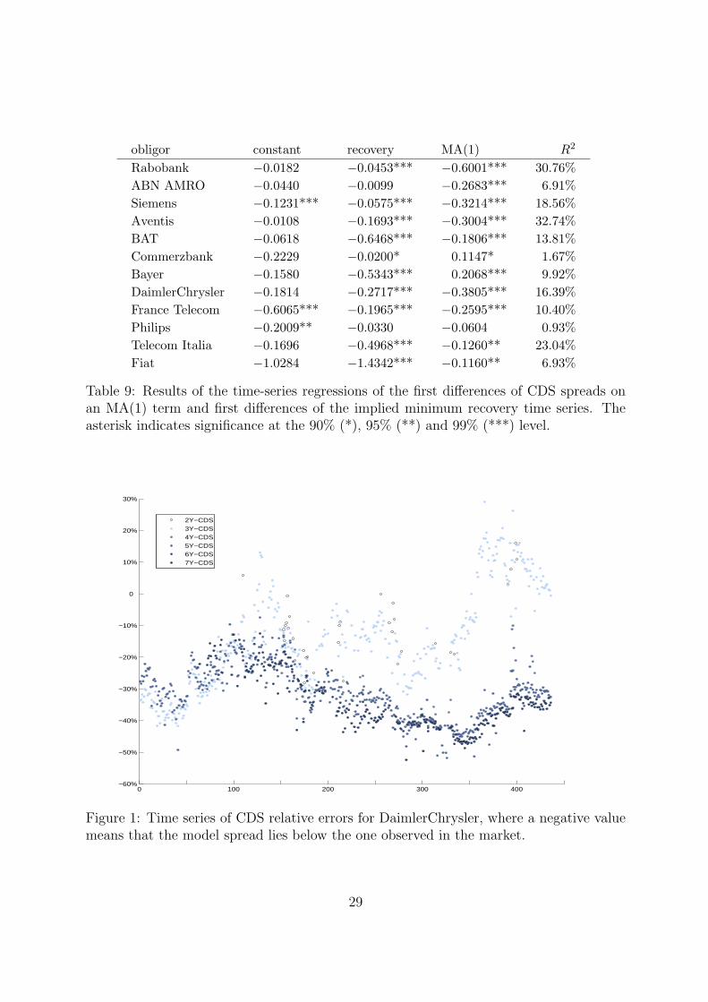
On average the mean absolute pricing error (MAE) is 24.30 bp or 23.92% expressed inrelation to the spread size, which constitutes a considerable mispricing. The mean relativeabsolute errors (MRAE) lie within a minimum of 10.25% and a maximum of 57.53% ofthe spread. Moreover, the mean pricing errors (ME) are biased: For eight obligors themodel CDS spread is lower on average then the market CDS spread, and higher for fourobligors. The mean difference between model and market CDS spreads is thus negativeand tends to increase with lower rating grades when measured in basis points, but notwhen measured as a percentage of the market spread. Figure 1 shows the time series ofCDS pricing errors for the different maturities for DaimlerChrysler as a representativeexample.

The findings are qualitatively in line with Houweling and Vorst [16] and Blanco,

11

Brennan and Marsh [6], but opposed to the CDS basis reported in Longstaff,Mithal and Neis [21], where the model-independent CDS spread, proxied by the bondspread, turns out higher than the market CDS spread, with the difference getting morepronounced for lower rating grades. The lack of pricing accuracy in the CDS market thusobviously necessitates an extension of the standard setup to obtain a credit risk modelable to accurately price CDS and bonds at the same time. In the next section we thereforediscuss potential extensions and motivate our decision to model the delivery option of theCDS contract.

3 Modelling Extension

The literature proposes a multitude of potential factors for explaining the origin of thedifferences in the pricing between the bond and CDS markets. As mentioned in theintroductory section, these are put forward e.g. in studies by Hjort et al. [15] andO’Kane and McAdie [23], though in a purely descriptive manner. The explanatoryfactors most often cited in the literature are liquidity and the delivery option, the restbeing even less tangible.

3.1 Liquidity vs Delivery Option

The traditionally popular explanation for real-world market imperfections – liquidity –has hitherto already been thoroughly analyzed in the literature, yet with conflicting con-clusions. The studies fail to unambiguously answer several crucial questions: First of all,it is still unclear whether liquidity actually presents a valid explanation in the first placesince the arguments produced could affect spreads either way, i.e. which market shouldbe more liquid than the other and why. Even after accepting liquidity as the driver of themispricings, it remains unresolved whether the difference in liquidity is perhaps betweenCDS and bonds of single maturities rather than between the markets as a whole, whetherthe level of (relative) liquidity alternates with time between the two markets and/or be-tween instruments, or whether the bond and CDS markets for similar issuers (e.g. of aparticular rating) must exhibit similar relative liquidity properties.

The paper by Janosi, Jarrow and Yildirim [19] reveals the difficulty: Theircalibrated convenience yield process exhibits a varying sign, which raises doubts on itsrelation to liquidity. Longstaff, Mithal and Neis [21] indeed report a dependence onliquidity proxies of their residual yield spread obtained by calibrating an extra discountprocess to corporate bonds; since in addition they report an overestimation of CDS spreadsbefore adjusting for liquidity – which is in contrast to most other studies – our conjectureis that both the observed direction of the mispricings and the liquidity dependence are inall likelihood attributable to the specific data set used. Their argument would unlikelyhold for the data sets analyzed in Houweling and Vorst [16], Blanco, Brennanand Marsh [6] and Janosi, Jarrow and Yildirim [19]. The data set at our disposal

12

displays mispricings in line with the ones reported in Houweling and Vorst [16] andBlanco, Brennan and Marsh [6], and furthermore it turns out that liquidity proxiesdo not possess any explanatory power (cf. Section 3.4).

For the stated reasons this paper considers the delivery option as an alternative expla-nation for the mispricing between the bond and CDS market stemming from the mannerin which a CDS is usually settled in default. Since the form of settlement prevailing inthe CDS market by far is physical delivery of defaulted assets (in contrast to cash set-tlement), one must examine its implications for CDS pricing. Namely, a CDS contractcommonly refers not to one single deliverable obligation only, but to a basket of deliv-erable obligations satisfying certain conditions, the crucial one being the seniority of thedebt delivered. As illustrated by event studies in Section 3.2, contrary to the commonmodelling assumption of equal bond prices in default, the differences between post-defaultprices of deliverable bonds cannot be ignored.

One conceivable origin of differing bond values in and after default is put forth in arecent theoretical paper by Guo, Jarrow and Zeng [14] for instance, who develop areduced-form model based on the idea that a default does not need to immediately leadto bankruptcy. According to their definition, the issuer continues to operate after defaultdepending on whether she is solvent or not. As a result, the issuer’s bonds continueto exist as well, and trade at different levels depending on their characteristics (couponand maturity). Studies by Guha [13] or Duffie and Singleton [10] also suggest thatbond prices at default could reflect market expectations whether the obligor will continueoperating after the credit event or rather be liquidated straight away. Another possibleorigin could be deduced for example from particular supply and demand considerationsin default, e.g. when one market participant is accumulating debt of a defaulted borrowerto influence the outcome of the bond settlement process. A third origin of differing bondprices in and after default could arise from trading frictions (e.g. high transaction costs)and market imperfections (e.g. the impossibility of shorting), which induce individualbonds to trade away from their supposedly fair values. Bond pricing errors as calculatedin Section 2.6 are a possible indicator of such deviations.

The protection buyer thus possesses an option to deliver the cheapest bond(s) upondefault. Obviously, the spread at the inception of the CDS contract must reflect theuncertain recovery values (i.e. bond prices) in default, additionally to capturing the defaultrisk of the borrower. The common modelling assumption of a recovery value which isconstant and identical across both markets has several consequences: For one, it impliesthat bond prices are equal in default, making the delivery option worthless. Moreover,such a recovery rate forces the CDS spread to be driven exclusively by the default riskof the underlying, as can be clearly discerned from Eq. (3), potentially causing unnaturalfluctuations in the implied default intensity. Lastly, from a modelling point of view,plugging in constant recovery rates precludes the analysis of their mutual dependence onthe default intensities.

As observed in Section 2.6, mispricing arises when equal recovery values are used in

13

the bond and CDS markets. The aim of the present paper is to analyze whether theinclusion of variable CDS recovery values representing the cheapest-to-deliver bond pricein default can bring about pricing effects and explain the emergence of the CDS basis.

3.2 Case Studies of Defaults

For the purpose of verifying the conjecture that the delivery option potentially possessesvalue, we inspect the behavior of bond prices during the time period immediately beforeand after default for three companies which filed for Chapter 11 bankruptcy protectionduring 2005. The obligors are Delta Air Lines, Inc. and Northwest Airlines, Inc., whichfiled for Chapter 11 on Wednesday, September 14th, 2005, and Delphi Corp., which filedfor Chapter 11 on Saturday, October 8th, 2005. Price quotations from Bloomberg are atour disposal for four (senior unsecured) bonds issued by Delta and Northwest Airlines eachand for three (senior unsecured) bonds of Delphi. The price information is available for thewhole month in which the respective defaults occurred and consists of the mid-quotationsof the daily low, high and closing prices for each bond.

Figure 2 shows the daily average closing prices for each company in its month ofdefault. The default event had a clear impact on the bond prices of Northwest andDelphi, whereas the default of Delta apparently happened as no surprise to the marketsince it had no noticeable effect on bond prices. Comparing the average closing prices atdefault, we observe that the price levels of the three obligors are quite dispersed: Deltahad the lowest price level with an average bond price of 15.92 (per 100 of face value),followed by Northwest with 26.81 and Delphi with 57.92. These figures point at highvariations in the recovery between different corporate defaults.

Since the delivery option in a CDS is worthless in default if bond prices of the companycoincide, our main interest lies in comparing the individual bond prices of each obligor todetect their potential discrepancies. In the ideal case one seeks to compare price informa-tion for different bonds obtained at exactly the same points in time. Since only the dailylow, high and closing prices for each bond are at our disposal, we are merely able to infercertain bounds on the contemporaneous maximum price differences, as described below.Closing prices provide some indication of contemporaneous price differences, though withtwo drawbacks: First, closing prices might not be contemporaneous since the end-of-dayvalues could stem from different points in time during the trading day, and second, intra-day price deviations might be both lower and higher than suggested by closing prices.Information on the intra-day price differences is therefore inferred by looking at the dailylow and high of each bond price.

Let us assume for a moment that an obligor has only two bonds outstanding on defaultday, bond A and bond B. We have at our disposal the high and low for both bonds ondefault day. Without loss of generality, let bond A have the smaller low price. In theperiod during this trading day when bond A was at its low, bond B was by definitiontrading at a price greater or equal to its own low. It follows that if the difference between

14

these lows is non-zero, there must have existed a period during the day when the pricedifference between these bonds was at least that much. For this reason we term this valuethe lower bound of the contemporaneous (maximum) price differences. On the other hand,bond B traded at most at its own high price on this day, and especially in the period whenbond A was at its low. The difference between these values is thus an upper bound onthe contemporaneous price differences. This is the highest possible price difference whichmight have been realized on this day. The case with more than two bonds outstandingat the time of default is analogous. In order to infer the lower bound we compare themaximum and the minimum of the bonds’ low prices, and for the upper bound we considerthe maximum of the highs and the minimum of the lows.

Table 5 contains the bounds for the contemporaneous price difference for each obligoron its day of default. For Delta Airlines the values are in the range between 4.42 and 8.67,and the dispersion of closing prices amounts to 1.81. For Delphi the price differences areof comparable magnitude with 1.50 between closing prices, a lower bound of 3.00, and anupper bound of 8.50. For Northwest Airlines the differences are even higher with a 6.00difference between closing prices, a 3.39 lower bound, and a 12.40 upper bound. Overall,we find substantial contemporaneous price deviations in the range of 3 to 12, stronglyindicating that the delivery option is valuable and requires further consideration.

Since on the one hand the default event is anticipated by the market for some obligors,e.g. Delta Airlines, and on the other hand the settlement period for CDS contracts lasts30 days following a default, price differences before and after default are of additionalinterest. Figure 3 shows the daily lower and upper bounds of the price differences in themonth of default for each company. The price differences before and after default arequite similar for Delta Airlines and Delphi, whereas for Northwest Airlines significantlyhigher differences are observed before default possibly because it happened as a surpriseto the market. After default, the lower bounds are in the range of 1 to 8 and the upperbounds are between 3 and 14 for all companies, strengthening the argument against equaldefault prices. Furthermore, bond prices vary strongly over time after the default event:Comparing the maximum high and the minimum low of bond prices over the post-defaultperiod (cf. Table 5) yields 9.6 vs. 22 for Delta Airlines, 19.5 vs. 32 for Northwest Airlines,and 49.2 vs. 70.5 for Delphi.

The findings described above are in line with the ones in a more comprehensive studyof corporate defaults by Guha [13]. Upon closer inspection of Table VIII in the citedpaper, which shows the bond-price ranges of all obligors in the sample on default day, onefinds that obligors with a price range wider than one dollar are almost as numerous as theones with prices converging to approximately the same value (i.e. price range within onedollar). Incomprehensibly, the author claims that “in the vast majority of cases bondsof the same issuer and seniority are valued equally or within one dollar by the market,irrespective of their time to maturity” [13, p. 21, emph. added]. This claim obviouslycontradicts his observations, the more so as bond price differences in default are likelyto be even higher when focusing only on the subset of obligors which are actively tradedin the CDS market and taking into account not just their day of default, but the whole

15

period up to the CDS settlement day.

In this case study we have uncovered substantial bond price differences both contem-poraneously and over time, showing the complex stochastic nature of recovery rates. Thefindings indicate that the delivery option is potentially valuable and thus needs to beexplicitly accounted for in credit risk models. One drawback of our case study is that thedata only include mid-prices, but the deviations of the individual bonds are neverthelessobvious and should hold when the bid-ask spread is included.

3.3 Extended Methodology

As discussed in the preceding sections, within the reduced-form framework little hasbeen written on the implementation of recovery rate models although they are equally assignificant to the accuracy of a credit risk model as is the default likelihood. Hence, sincethe aim of this paper is to analyze the influence of the delivery option, we are compelledto go beyond the customary model, which implicitly ignores its existence.

The prevailing intensity-based model values bonds and CDS with the same underlyingcredit risk using a constant recovery parameter equal for both markets, usually inferredfrom surveys of historically realized recovery rates such as Altman, Resti and Sironi[1]. This is exactly the setup we adopted in our basic analysis in Section 2, finding out thatit is inadequate for simultaneous pricing in both the underlying and derivatives market.

Going beyond the usual model means that we need to induce uncertainty in the recov-ery rates of bonds at the time of default. Formally, a straightforward way of achieving thisgoal within the reduced-form framework is augmenting the Poisson (one-point) processmodelling the survival and default of an obligor by a vector of random markers represent-ing the recovery rates of bonds and drawn at the time of default. In this respect our setupbuilds on Schonbucher [24]. Based on a general model exhibiting random recovery ratesas a motivation for our approach, we deduce and justify the assumptions adopted in thesubsequent empirical analysis in order to reduce the parameters to a computationallytractable number.

Taking one step back, not only are realized recovery rates among bonds in defaultdifferent, but there is another source of randomness driving the correct recovery parameterin the pricing of CDS – the number of deliverable bonds outstanding at the time of default.Buhler and Dullmann [5] face a similar problem when developing a conversion factorsystem for a multi-issuer bond futures contract. The paper conveniently assumes that theclearing house pledges to substitute defaulted bonds by bonds of similar characteristics inorder to avoid dealing with a random number of deliverable bonds. Analogously, we alsomake the assumption that the number of deliverable bonds, K, is constant and known atinception of the CDS contract. It can be argued that the firms in the sample are matureenough to have reached a balanced number of outstanding debt instruments over time,so though some debt may mature before the maturity of the CDS, in all likelihood newdebt will be issued instead. Based on this assumption we next present our methodology.

16

Denote by G(t, dπ) the K-dimensional distribution (under the martingale measure Q)on [0, 1]K of the random vector π of recovery rates conditional on default happening in theinfinitesimal time interval 〈t, t + dt]. The randomness is introduced ad hoc because thepresent literature does not yet agree about which fundamental factors (such as the firm’sasset value, bond maturity or coupon amount) influence the bond value at default andhow. For this reason we deliberately leave aside the potential origin of the differences inrecovery rates wanting to focus rather on their consequences for now. The only technicalrequirement placed on this distribution is integrability with respect to the martingalemeasure Q.

The only part of the bond valuation formula (1) affected by these considerations isthe recovery payment in default. In full generality, the time-t value of the now randomrecovered amount πk(τ) on bond k, 1 ≤ k ≤ K, with maturity T k is expressed as:

EQt

[πk(τ) P (t, τ) 1t<τ≤T k

]=

∫ T k

t

∫[0,1]K

πk(s) P (t, s) Q(t, s) G(s, dπ) λ(s) ds

=

∫ T k

t

πek(s) P (t, s) Q(t, s) λ(s) ds ,

where πek(t) :=

∫[0,1]K

πk(t) G(t, dπ) denotes the locally (i.e. time-t) expected recovery rate

for bond k.

In general, it is justified to use the locally expected recovery rate when pricing acorporate bond because its payoff depends linearly on the recovery rate – as is convenientlythe case with both bonds and CDS, but is violated e.g. by recovery swaps.

The modeler is now free to choose the (deterministic) locally expected recovery func-tion she deems appropriate, though data availability poses considerable constraints, ren-dering impossible a calibration of both the intensity function and an elaborate recoveryfunction (potentially even separately for each of the bonds), which leads us to adopt thefollowing simplifying assumption when pricing bonds:

Assumption 1. (bonds)All one-dimensional marginal distributions of the vector of recovery rates have identicalexpectations regardless of the timing of default:

πek(t) = πe ∈ [0, 1] for all 1 ≤ k ≤ K and t ≥ 0.

Since we are only looking at bonds of a single seniority this assumption makes senseeconomically nevertheless: Though bonds in the same class are expected to recover iden-tical amounts in the event of default, the actual realizations need not be equal. Notealso that the assumption corresponds to our recovery specification in the basic model (cf.Section 2).

Having dealt with bond valuation under random recovery, we next turn to CDS pricing.The default-contingent payoff of a CDS contract with physical delivery depends on the

17

value of the cheapest-to-deliver bond, i.e. on the minimum recovery rate over all deliverableobligations at the time of default:

πmin(τ) = min1≤k≤K

πk(τ).

Analogously to the above, only the default-contingent loss payment in a CDS is affectedby these considerations. In full generality, the present value of the now random losscompensation 1− πmin(τ) in a CDS with maturity T is expressed as

EQt

[(1− πmin(τ)) P (t, τ) 1t<τ≤T

]=

∫ T

t

∫[0,1]K

(1− πmin(s)) P (t, s) Q(t, s) G(s, dπ) λ(s) ds

=

∫ T

t

(1− πemin(s)) P (t, s) Q(t, s) λ(s) ds ,

where πemin(t) :=

∫[0,1]K

πmin(t) G(t, dπ) denotes the locally (i.e. time-t) expected minimumrecovery rate.

Once more, the modeler is now free to choose an appropriate (deterministic) locallyexpected minimum recovery function, but the data pose restrictions again. Therefore, weabstain from calibrating a complex minimum recovery function, but adopt the followingsimplifying assumption when pricing CDS in the extended setting:

Assumption 2. (CDS)The distribution of the locally expected minimum recovery rate has identical expectationsregardless of the timing of default:

πemin(t) = πe

min ∈ [0, 1] for all t ≥ 0.

πemin therefore represents the expected value of the cheapest-to-deliver bond, identical

for all possible default times. Thus, the main consequence of our extension is that theexpected recovery rate for each bond πe and the expected minimum recovery rate πe

min inthe CDS are now allowed to differ.

In the implementation, we fix the recovery rate for each individual bond (at 40%) asin standard credit risk models. Additionally the implied minimum recovery parameteris calibrated to CDS data. For the purpose of measuring the influence of the deliveryoption this parameterization is sufficient, since the implicit value of the delivery option isreflected by the difference in the recoveries.

We calibrate the implied minimum recovery parameter every day to CDS data ofeach issuer. Suppressing the issuer and day indices, let there be J CDS available withobservable market quotes pmkt

j , 1 ≤ j ≤ J . The implied expected minimum recovery

18

parameter is obtained by minimizing the mean absolute CDS pricing errors of the model:

πemin = arg min

π∈[0,1]

1

J

J∑j=1

∣∣pmkt

j − pj(·, tjn, π; θ∗)∣∣ ,

where θ∗ is the parameter vector of the Nelson-Siegel model already calibrated to bondprices (cf. Section 2.5). As previously, the estimation is implemented via non-linear opti-mization.

3.4 Results

The average implied minimum recovery lies in the range between 8.87% and 46.34% (cf.Table 6) and exhibits substantial dispersion among the analyzed obligors. It stronglyvaries even within an individual rating and industry class, thereby strengthening our ar-gument for a firm-specific delivery option. The average standard deviation of the impliedrecovery values is approximately 10%, indicating significant fluctuation over time. Figure4 shows the time series of the implied minimum recovery rate estimated for Daimler-Chrysler and is representative of the time-series properties for the whole sample. Theimplied recovery for DaimlerChrysler averages 11.5% and exhibits a seemingly cyclical ormean-reverting behavior over time.

The findings indicate that the effect of the delivery option on the CDS spread is strongenough to result in plausible implied recovery values, i.e. one does not observe a dominanceof boundary solutions (0% or 100%) which would suggest that the delivery option cannotexplain the CDS pricing errors and thus does not drive CDS spreads. Considering thelowest and highest implied minimum recovery in the time series per obligor (cf. Table 6),the value of 100% is never estimated as the optimal parameter, whereas for half of theobligors the value of 0% is estimated at least once, which could be deemed too low andcould indicate that effects other than the delivery option may be at work, which are alsoreflected in the calibrated recovery parameter.

Basically, these additional effects could have been introduced by the simplifying as-sumptions on the recovery parameter. One effect may be a dependence of the minimumrecovery on the CDS maturity because for CDS with longer maturities not all bondsmight be available for delivery in default as some may mature without being replaced.Furthermore, the default intensity and the recovery rate could be correlated in reality.Finally, the implied recovery parameter could be driven by other factors, such as liquidity.All these effects potentially influence the calibrated implied recoveries. For this reason,we conduct a cross-sectional analysis of the implied recoveries to demonstrate that thisparameter is primarily driven by the value of the delivery option.

Modelling the delivery option by introducing the implied minimum recovery rate weexpect a significant improvement in pricing ability for the CDS market. Table 7 documentsthe pricing performance of the extended model on CDS. The average MAE is reduced from

19

24.3 bp to 7.9 bp, resp. from 23.6% to 11.1% expressed as relative error. Compared to therange of bid-ask spreads of 3 to 10 bp (with the exception of Fiat, where bid-ask spreadsare up to 40 bp), these pricing errors seem acceptable, which is a crucial improvement withrespect to the initial model. From a technical point of view pricing errors are naturallyexpected to decrease by adding a further parameter to the model, so as a next step it isessential to demonstrate that the additional parameter possesses an economic justification.

To this end, we investigate whether the implied recovery rates are linked to factorsdriving the value of the delivery option by taking a regression-based approach. Liquidityproxies are taken into account as control variables in order to test whether liquidity affectsthe estimated recovery rates. The following list presents the presumptive proxies for thevalue of the delivery option and our hypotheses for their influence on the implied minimumrecovery:

number of bonds:The more bonds available for delivery, the lower the expected minimum price indefault, which is exactly the recovery of the cheapest-to-deliver bond. In our dataset the average number of available bonds per obligor is in the range from two toseven bonds.

maximum bond price difference:The maximum bond price difference is defined as the difference between the highestand the lowest market bond price. If the difference persists in default, corporateswith higher price differences will exhibit lower implied recovery rates. In our samplethe average maximum bond price differences lie in the range from 2.56 to 15.74.

absolute bond pricing error:In principle, pricing errors indicate that there exist bonds whose market values de-viate from their model prices. If the magnitude of the deviations persists in default,corporates with higher bond absolute pricing errors will exhibit lower implied re-covery rates. As displayed in Table 7, in our sample the bond MAE is in the rangefrom 0.24 bp to 39.06 bp.

minimum bond pricing error:The minimum bond pricing error is defined as the pricing error of the bond with thelargest deviation below its model price. If the magnitude of the deviations persistsin default, corporates with higher minimum bond pricing errors will exhibit lowerimplied recovery rates. In our sample the average minimum bond pricing errors fallin the range from 0.003 bp to 63.6 bp.

The following liquidity proxies are also included in the regressions: the average bid-askspread (between 18.07 bp and 78.03 bp), the notional amount outstanding (in the range0.6 bn to 2.5 bn euro), the average bond coupon (4.34% to 6.27%) and the rating (cf.Table 2), all employed in Longstaff, Mithal and Neis [21] as well.

20

Time averages of the implied minimum recovery values and all explanatory variablesare determined for each obligor and the implied recovery rate is cross-sectionally regressedseparately against each proxy. Table 8 presents the regression statistics. All four variablesrepresenting the delivery option are both statistically and economically significant, andthe hypothesized sign of the respective coefficients is confirmed. Based on the R2, thenumber of bonds and the minimum bond pricing errors have the highest explanatorypower. Interpreting the influence of these two factors, it follows that the implied minimumrecovery decreases by 6% on average if an additional bond is available, and by 5.4% onaverage if the minimum bond pricing error increases by 10 bp. Due to the small cross-section of only twelve obligors, one needs to examine whether the significance of theparameters in the regressions possibly stems from outliers. To this end, we plot the datasets and lay the respective regression lines on top, but no indication of such misfitting isfound. As a representative example the scatter plot of the average implied recovery rateagainst the number of bonds is included in Figure 5.

On the other hand, all four variables representing liquidity are statistically insignificantand not even close to the 90% confidence interval, indicating that in our sample there isno serious influence of liquidity on the estimated implied recovery rates – at least not theway we measure it. The importance of including the delivery option into credit pricingmodels is thereby further strengthened. As a consistency check the time series is splitinto two parts (2003 and 2004), and the cross-sectional regression analysis repeated onboth subperiods, but the results stay virtually the same (details not reported).

Finally, a time series analysis is performed for each obligor to explore the effect of theimplied recovery rate on the CDS spread. Since the CDS spread is driven both by defaultrisk and by recovery risk, the implied recovery rate is expected to account for part of theobserved variation in CDS spreads over time, i.e. an increase in the recovery rate shouldresult in a decrease of the CDS spread. To explore this relation we specify a univariatetime series model for the CDS spread and include the recovery rate as an explanatoryvariable. The autocorrelation structure of CDS spreads is taken into account by modellingfirst differences as an MA(1) process. First differences of the implied recovery rate areadded to this model setup as an explanatory variable. Table 9 contains the main regressionstatistics. The coefficients of the implied recovery rate exhibit the expected negative signfor all obligors, meaning that a decrease in the implied recovery rate induces an increase inthe CDS spread, and for ten out of twelve obligors the implied recovery rate is significantfor explaining the CDS spread (even after accounting for autocorrelation effects, whichitself could be caused by recovery risk). Lastly, one notices that there exist differences inthe relative importance of default risk and recovery rate risk for the individual obligors,as indicated by the differing R2 levels.

21

4 Conclusion

The tremendous growth rates and the increasing diversity of products in the credit riskmarket are continuously calling for the development of more and more sophisticated pric-ing methods. As shown in recent academic studies, under standard assumptions reduced-form credit risk models are not fully capable of accurately pricing the two fundamentalcredit risk instruments – bonds and credit default swaps (CDS) – simultaneously.

Using a data set of euro-denominated corporate bonds and CDS this paper quantifiesthe mispricing observed when employing a deterministic reduced-form framework. In anextensive comparison of the pricing properties in the bond market for several parameter-izations of the default intensity the Nelson-Siegel specification turns out to be optimal.This parametrization is subsequently used to price CDS, resulting in model CDS spreadsup to 50% lower on average than observed in the market.

The traditionally popular explanation for real-world imperfections in credit markets –liquidity – has already been thoroughly analyzed in academic literature, yet with conflict-ing conclusions. The studies fail to unambiguously answer questions such as which marketis more liquid or whether liquidity is priced at all. In this paper an alternative extensionis therefore presented which models the delivery option implicit in CDS contracts: Sincein default a basket of bonds is deliverable, the effect of the cheapest-to-deliver bond priceneeds to be accounted for in CDS valuation. By using a constant recovery rate standardcredit risk models assume equal recoveries for all bonds, and hence implicitly assume zerovalue for the delivery option.

Contradicting this common modelling assumption, case studies of recent Chapter 11filings presented in this paper illustrate that bonds of a defaulted obligor do not tradeat equal levels following default. Our extension therefore models the implied expectedrecovery rate of the cheapest-to-deliver bond and, applied to the data, it largely eliminatesthe mispricing. The calibrated recovery values lie in the range between 8% and 47% forthe different obligors, exhibiting strong variation among rating classes and industries. Across-sectional analysis reveals that the implied recovery parameter depends on proxiesfor the delivery option: The variables with the highest explanatory power are the numberof available bonds and the bond pricing errors. No evidence is found for the influence ofliquidity proxies.

Our paper thus points out the necessity for incorporating the random structure ofrecovery rates at default into credit risk models in order to accurately price credit-riskyinstruments.

22

References

[1] E. Altman, A. Resti, A. Sironi, Default Recovery rates in Credit Risk Modelling: AReview of the Literature and Empirical Evidence, Economic Notes by Banca Montedei Paschi di Siena SpA, Vol. 33 (2004), No. 2.

[2] D. Aunon-Nerin, D. Cossin, T. Hricko, Z. Huang, Exploring for the Determinants ofCredit Risk in Credit Default Swap Transaction Data: Is Fixed-Income Markets’ In-formation Sufficient to Evaluate Credit Risk?, FAME Research Paper No. 65 (2002).

[3] G. Bakshi, D. Madan, F. Zhang, Understanding the Role of Recovery in Default RiskModels: Empirical Comparisons and Implied Recovery Rates, Working Paper (2001).

[4] C. Benkert, Explaining Credit Default Swap Premia, Journal of Futures Markets, Vol.24 (2004), No. 1.

[5] W. Buhler, K. Dullmann, Conversion Factor Systems and the Delivery Option of aMulti-Issuer Bond Future, Working Paper (2005).

[6] R. Blanco, S. Brennan, I.W. Marsh, An Empirical Analysis of the Dynamic Relationbetween Investment-Grade Bonds and Credit Default Swaps, Journal of Finance, Vol.60 (2005), No. 5.

[7] P. Collin-Dufresne, R.S. Goldstein, J.S. Martin, The Determinants of Credit SpreadChanges, Journal of Finance, Vol. 56 (2001), No. 6.

[8] D. Duffie, Credit Swap Valuation, Financial Analysts Journal, Jan./Feb. Issue (1999).

[9] D. Duffie, L.H. Pedersen, K.J. Singleton, Modeling Sovereign Yield Spreads: A CaseStudy of Russian Debt, Journal of Finance, Vol. 53 (2003), No. 1.

[10] D. Duffie, K.J. Singleton, Modeling Term Structures of Defaultable Bonds, Review ofFinancial Studies, Vol. 12 (1999), No. 4.

[11] P. Feldhutter, D. Lando, Decomposing Swap Spreads, Working Paper (2005).

[12] A. Geyer, S. Kossmeier, S. Pichler, Measuring Systematic Risk in EMU GovernmentYield Spreads, Review of Finance, Vol. 8 (2004), No. 2.

[13] R. Guha, Recovery of Face Value at Default: Theory and Empirical Evidence, Work-ing Paper (Dec. 2002).

[14] X. Guo, R.A. Jarrow, Y. Zeng, Modeling the Recovery Rate in a Reduced Form Model,Working Paper (Sep. 2005).

[15] V. Hjort, S. Dulake, M. Engineer, N.A. McLeish, The High Beta Market – Exploringthe Default Swap Basis, Morgan Stanley Credit Derivative Strategy Special Report(2002).

23

[16] P. Houweling, T. Vorst, Pricing Default Swaps: Empirical Evidence, Journal of In-ternational Money and Finance, Vol. 24 (2005), No. 8.

[17] J.C. Hull, M. Predescu, A. White, Bond Prices, Default Probabilities and Risk Pre-miums, Journal of Credit Risk, Vol. 1 (2005), No. 2.

[18] International Swaps and Derivatives Association, Inc., 2003 ISDA Credit DerivativesDefinitions.

[19] T. Janosi, R. Jarrow, Y. Yildirim, Estimating Expected Losses and Liquidity Dis-counts Implicit in Debt Prices, Working Paper (2002).

[20] R. Jarrow, Default Parameter Estimation Using Market Prices, Financial AnalystsJournal, Sep./Oct. Issue (2001).

[21] F.A. Longstaff, S. Mithal, E. Neis, Corporate Yield Spreads: Default Risk or Liquid-ity? New Evidence from the Credit Default Swap Market, Journal of Finance, Vol.60 (2005), No. 5.

[22] E. de Malherbe, A Simple Probabilistic Approach to the Pricing of Credit DefaultSwap Covenants, Journal of Risk, Vol. 8 (2006), No. 3.

[23] D. O’Kane, R. McAdie, Explaining the Basis: Cash versus Default Swap, LehmanBrothers Structured Credit Research (2001).

[24] P.J. Schonbucher, Credit Derivatives Pricing Models: Models, Pricing and Imple-mentation., John Wiley & Sons, 2003.

[25] H. Zhu, An Empirical Comparison of Credit Spreads Between the Bond Market andthe Credit Default Swap Market, BIS Working Paper No. 160 (2004).

24

functional forms free parameters

linear α0 + α1t 2

quadratic α0 + α1t + α2t2 3

cubic α0 + α1t + α2t2 + α3t

3 4

log-linear α0 + α1t + κ1

1+t3

Nelson-Siegel β0 + β1e− t

κ1 + β2t

κ1e− t

κ1 4

Svensson β0 + β1e− t

κ1 + β2t

κ1e− t

κ1 + β3t

κ2e− t

κ2 6

Table 1: Specifications of the intensity function examined. αi, βi and κi denote themodel parameters satisfying the usual constraints for the Nelson-Siegel and Svenssonparameterizations. The term log-linear applies here to the integrated intensity function.

obligor Moody’s rating industry

Rabobank Aaa Banking

ABN AMRO Aa3 Banking

Siemens Aa3 Electrical Equipment

Aventis A1 Pharmaceuticals

British American Tobacco (BAT) A2 Tobacco

Commerzbank A2 Banking

Bayer A3 Pharmaceuticals

DaimlerChrysler A3 Automobiles

France Telecom A3 Telecom

Philips Baa1 Electronics

Telecom Italia Baa2 Telecom

Fiat Ba3 Automobiles

Table 2: Obligors selected for the study with corresponding rating and industry.

25

obligor linear quadratic cubic log-linear Nelson-Siegel SvenssonRabobank 16.32 bp 15.01 bp 15.76 bp 17.39 bp 15.35 bp 15.58 bpABN AMRO 7.27 bp 4.47 bp 7.37 bp 5.01 bp 9.59 bp 5.81 bpSiemens 3.64 bp 1.97 bp 5.52 bp 0.14 bp 1.22 bp 3.62 bpAventis 4.47 bp 4.22 bp 4.12 bp 0.14 bp 0.24 bp 1.30 bpBAT 47.08 bp 17.40 bp 8.84 bp 11.19 bp 5.65 bp 2.01 bpCommerzbank 9.05 bp 7.27 bp 8.77 bp 9.70 bp 13.16 bp 11.63 bpBayer 35.58 bp 17.39 bp 15.08 bp 8.36 bp 1.70 bp 3.92 bpDaimlerChrysler 56.13 bp 36.66 bp 12.83 bp 10.50 bp 9.37 bp 7.62 bpFrance Telecom 32.04 bp 16.10 bp 16.24 bp 46.88 bp 15.23 bp 16.67 bpPhilips 26.00 bp 10.98 bp 9.78 bp 7.17 bp 2.15 bp 3.10 bpTelecom Italia 43.04 bp 22.13 bp 18.76 bp 13.87 bp 2.78 bp 3.69 bpFiat 216.43 bp 152.49 bp 44.18 bp 48.64 bp 39.06 bp 33.25 bpoverall 41.42 bp 25.51 bp 13.94 bp 14.92 bp 9.62 bp 9.02 bp

Table 3: Mean absolute pricing errors (MAE) for the bonds of each obligor over the periodexamined for the six specifications of the intensity function.

bonds CDSobligor ME MAE ME MRE MAE MRAERabobank −0.98 bp 15.35 bp −5.03 bp −52.48% 5.51 bp 57.53%ABN AMRO 0.52 bp 9.59 bp −2.12 bp −12.25% 3.02 bp 17.41%Siemens −1.22 bp 1.22 bp −5.73 bp −19.78% 8.04 bp 27.73%Aventis −0.24 bp 0.24 bp 4.95 bp 26.90% 5.11 bp 27.74%BAT −2.06 bp 5.65 bp 6.85 bp 9.53% 7.37 bp 10.25%Commerzbank −2.18 bp 13.16 bp −8.62 bp −26.31% 9.17 bp 28.02%Bayer −1.69 bp 1.70 bp 6.36 bp 10.60% 7.26 bp 12.10%DaimlerChrysler −1.69 bp 9.37 bp −26.83 bp −28.80% 27.27 bp 29.27%France Telecom −1.55 bp 15.23 bp −13.62 bp −16.30% 14.52 bp 17.37%Philips −1.55 bp 2.15 bp 0.56 bp 1.01% 6.23 bp 11.21%Telecom Italia −1.11 bp 2.78 bp −4.80 bp −5.93% 8.43 bp 10.40%Fiat −5.38 bp 39.06 bp −186.80 bp −37.38% 189.63 bp 37.95%overall 9.62 bp 24.30 bp 23.92%

Table 4: Pricing properties over the period examined for the Nelson-Siegel specification ofthe intensity function. Reported are the mean pricing errors (ME) and the mean absolutepricing errors (MAE) of both bonds and CDS, as well as the mean relative pricing errors(MRE) and the mean relative absolute pricing errors (MRAE) for CDS. A negative valuemeans that the model price resp. spread lies below the one observed in the market.

26

Delta Northwest Delphi

Chapter 11 filing 14.09.2005 14.09.2005 08.10.2005Day of default 14.09.2005 14.09.2005 10.10.2005Observation period 09/2005 09/2005 10/2005

Contemporaneous (maximum) price differences on default day:

Closing price 1.81 6.00 1.50Lower bound 4.42 3.39 3.00Upper bound 8.87 12.40 8.50

Prices in the post-default period:

Minimum price 9.58 19.50 49.20Maximum price 22.00 32.00 70.50

Table 5: Summarized details of case studies of defaults (differences resp. prices per 100of face value).

mean std. dev. min maxRabobank 8.87% 18.72% 0.00% 73.61%ABN AMRO 35.34% 12.88% 0.00% 61.54%Siemens 31.86% 9.86% 0.00% 57.68%Aventis 46.11% 6.91% 24.50% 62.98%BAT 45.93% 4.37% 24.88% 74.86%Commerzbank 27.14% 13.32% 0.00% 58.87%Bayer 46.34% 4.97% 29.92% 71.11%DaimlerChrysler 11.48% 9.55% 0.00% 33.62%France Telecom 29.97% 6.78% 0.00% 73.10%Philips 43.91% 6.85% 31.34% 81.83%Telecom Italia 33.37% 8.14% 15.50% 52.65%Fiat 13.74% 13.42% 0.00% 53.19%

Table 6: Descriptive statistics of the implied minimum recovery rate.

27

bonds CDSobligor ME MAE ME MRE MAE MRAERabobank −0.98 bp 15.35 bp −3.23 bp −33.74% 3.55 bp 37.02%ABN AMRO 0.52 bp 9.59 bp −1.24 bp −7.15% 1.76 bp 10.15%Siemens −1.22 bp 1.22 bp −2.50 bp −8.64% 5.30 bp 18.27%Aventis −0.24 bp 0.24 bp 2.45 bp 13.31% 3.17 bp 17.23%BAT −2.06 bp 5.65 bp −0.71 bp −0.99% 0.75 bp 1.04%Commerzbank −2.18 bp 13.16 bp −3.18 bp −9.72% 3.35 bp 10.22%Bayer −1.69 bp 1.70 bp 0.55 bp 0.91% 1.78 bp 2.97%DaimlerChrysler −1.69 bp 9.37 bp 2.38 bp 2.56% 6.84 bp 7.34%France Telecom −1.55 bp 15.23 bp −3.57 bp −4.27% 6.75 bp 8.08%Philips −1.55 bp 2.15 bp −3.30 bp −5.94% 3.42 bp 6.16%Telecom Italia −1.11 bp 2.78 bp 1.54 bp 1.90% 2.63 bp 3.25%Fiat −5.38 bp 39.06 bp −46.96 bp −9.40% 55.04 bp 11.02%overall 9.62 bp 7.86 bp 11.06%

Table 7: Pricing properties over the period examined of the extended model. Reportedare the mean pricing errors (ME) and the mean absolute pricing errors (MAE) of bothbonds and CDS, as well as the mean relative pricing errors (MRE) and the mean relativeabsolute pricing errors (MRAE) for CDS. A negative value means that the model priceresp. spread lies below the one observed in the market.

constant coefficient p-value R2

nr of bonds 0.5481 −0.0634 0.0004 73.25%max. price difference 0.4865 −0.0237 0.0041 57.73%abs. bond error 0.3936 −0.0085 0.0168 45.07%min. bond error 0.4017 −0.0054 0.0025 61.47%bid-ask spread 0.3637 −0.0016 0.5732 3.28%principal 0.1702 0.0001 0.1693 17.99%coupon 0.2803 0.0060 0.9393 0.06%rating 0.3176 −0.0009 0.9514 0.04%

Table 8: Results of the univariate cross-sectional regressions of the implied minimumrecovery rate on proxies of the delivery option and liquidity.

28

obligor constant recovery MA(1) R2

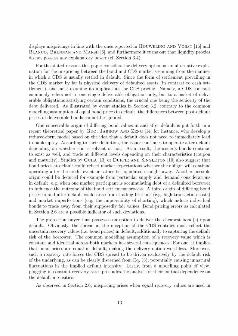
Rabobank −0.0182 −0.0453*** −0.6001*** 30.76%ABN AMRO −0.0440 −0.0099 −0.2683*** 6.91%Siemens −0.1231*** −0.0575*** −0.3214*** 18.56%Aventis −0.0108 −0.1693*** −0.3004*** 32.74%BAT −0.0618 −0.6468*** −0.1806*** 13.81%Commerzbank −0.2229 −0.0200* 0.1147* 1.67%Bayer −0.1580 −0.5343*** 0.2068*** 9.92%DaimlerChrysler −0.1814 −0.2717*** −0.3805*** 16.39%France Telecom −0.6065*** −0.1965*** −0.2595*** 10.40%Philips −0.2009** −0.0330 −0.0604 0.93%Telecom Italia −0.1696 −0.4968*** −0.1260** 23.04%Fiat −1.0284 −1.4342*** −0.1160** 6.93%

Table 9: Results of the time-series regressions of the first differences of CDS spreads onan MA(1) term and first differences of the implied minimum recovery time series. Theasterisk indicates significance at the 90% (*), 95% (**) and 99% (***) level.

0 100 200 300 400−60%

−50%

−40%

−30%

−20%

−10%

0

10%

20%

30%

2Y−CDS3Y−CDS4Y−CDS5Y−CDS6Y−CDS7Y−CDS

Figure 1: Time series of CDS relative errors for DaimlerChrysler, where a negative valuemeans that the model spread lies below the one observed in the market.

29

Delta Airlines

01.09.2005 09.09.2005 16.09.2005 23.09.2005 30.09.200510

11

12

13

14

15

16

17

18

19

20

Northwest Airlines

01.09.2005 09.09.2005 16.09.2005 23.09.2005 30.09.200520

25

30

35

40

45

50

Delphi

03.10.2005 10.10.2005 17.10.2005 24.10.2005 31.10.200555

60

65

70

Figure 2: Daily average closing prices for bonds in the month of default. The vertical lineindicates the day of the Chapter 11 filing.

30

Delta Airlines

Northwest Airlines

Delphi

Figure 3: Daily lower and upper bound for the contemporaneous maximum bond pricedifferences in the month of default. The vertical line indicates the day of the Chapter 11filing.

31

100 200 300 400

5%

10%

15%

20%

25%

30%

35%

Figure 4: Time series of the implied minimum recovery rate for DaimlerChrysler.

1 2 3 4 5 6 7 85%

10%

15%

20%

25%

30%

35%

40%

45%

50%

average number of bonds per day

aver

age

impl

ied

min

imum

reco

very

rate

Figure 5: Cross-sectional scatter plot of the average implied minimum recovery rateagainst the average number of bonds per day.

32