Nanoscale

PAPER

Cite this: Nanoscale, 2015, 7, 10101

Received 29th March 2015,Accepted 29th April 2015

DOI: 10.1039/c5nr02012c

www.rsc.org/nanoscale

The defect level and ideal thermal conductivity ofgraphene uncovered by residual thermal reffusivityat the 0 K limit†

Yangsu Xie,a Zaoli Xu,a Shen Xu,a Zhe Cheng,a Nastaran Hashemi,a Cheng Denga andXinwei Wang*a,b

Due to its intriguing thermal and electrical properties, graphene has been widely studied for potential

applications in sensor and energy devices. However, the reported value for its thermal conductivity spans

from dozens to thousands of W m−1 K−1 due to different levels of alternations and defects in graphene

samples. In this work, the thermal diffusivity of suspended four-layered graphene foam (GF) is character-

ized from room temperature (RT) down to 17 K. For the first time, we identify the defect level in graphene

by evaluating the inverse of thermal diffusivity (termed “thermal reffusivity”: Θ) at the 0 K limit. By using

the Debye model of Θ = Θ0 + C × e−θ/2T and fitting the Θ–T curve to the point of T = 0 K, we identify the

defect level (Θ0) and determine the Debye temperature of graphene. Θ0 is found to be 1878 s m−2 for the

studied GF and 43–112 s m−2 for three highly crystalline graphite materials. This uncovers a 16–43-fold

higher defect level in GF than that in pyrolytic graphite. In GF, the phonon mean free path solely induced

by defects and boundary scattering is determined as 166 nm. The Debye temperature of graphene is

determined to be 1813 K, which is very close to the average theoretical Debye temperature (1911 K) of the

three acoustic phonon modes in graphene. By subtracting the defect effect, we report the ideal thermal

diffusivity and conductivity (κideal) of graphene presented in the 3D foam structure in the range of

33–299 K. Detailed physics based on chemical composition and structure analysis are given to explain the

κideal–T profile by comparing with those reported for suspended graphene.

1. Introduction

Graphene, a form of carbon with a monolayer honeycomblattice, has been the focus of extensive investigations since itsdiscovery in 2004. Due to a number of intriguing properties,such as extremely high electrical1 and thermal conductivity,2

mechanical strength to weight ratios,3 and large specificsurface area,4 graphene has become an attractive candidate forpromising applications in various areas. Potential grapheneapplications include lightweight and flexible touch screens,5

electric circuits,6 solar cells,7 next generation batteries,8 lowcost water desalination,9 drug delivery,10 etc. Understandingthe fundamental physics and the underlying mechanism con-trolling those amazing properties can pave the way for its wideapplications.

Among its numerous outstanding properties, the highestthermal conductivity (κ) is of significant importance for gra-phene’s applications. Different approaches have been develo-ped to characterize the thermal conductivity of graphene. Thefirst experimental measurement was conducted at the Univer-sity of California Riverside2 using a “noncontact techniquebased on micro-Raman spectroscopy”. In their experiment, anextremely high thermal conductivity of single-layered graphenewas found in a range of (4.84 ± 0.44) × 103 to (5.30 ± 0.48) × 103

W m−1 K−1 at RT. This value exceeds the measured thermalconductivity of other carbon materials, such as CNTs anddiamond. As for isotopically pure 12C graphene, the in-planethermal conductivity was determined to be higher than 4000W m−1 K−1 at 320 K by Chen et al. using the optothermalRaman technique.11 Despite the reported high conductivity,other smaller values were also obtained. Lee et al. performedmeasurements for suspended pristine SLG using Raman scat-tering spectroscopy. The resulting thermal conductivity is∼1800 W m−1 K−1 near 325 K to ∼710 W m−1 K−1 near 500 K.12

Faugeras et al. obtained value ≈630 W m−1 K−1 at a tempera-ture of about 600 K by employing micro-Raman scatteringexperiments for the suspended large graphene membrane.13

†Electronic supplementary information (ESI) available. See DOI: 10.1039/c5nr02012c

aDepartment of Mechanical Engineering, Iowa State University, Ames, IA 50011, USA.

E-mail: xwang3@iastate.edu; Tel: +1 515 2948023bSchool of Urban Development and Environmental Engineering, Shanghai Second

Polytechnic University, Shanghai 201209, P. R. China

This journal is © The Royal Society of Chemistry 2015 Nanoscale, 2015, 7, 10101–10110 | 10101

Publ

ishe

d on

01

May

201

5. D

ownl

oade

d by

Iow

a St

ate

Uni

vers

ity o

n 28

/05/

2015

14:

55:3

2.

View Article OnlineView Journal | View Issue

Their graphene membranes were obtained by depositing largegraphene crystals onto a silicon wafer. Many impuritiesresulted from the PMMA copper film and acetone may existdue to the sample fabrication process.

A large discrepancy exists between these experimentalresults. So far the value of the measured κ of graphene rangesfrom dozens to thousands of W m−1 K−1. The lower bound canbe further lowered for more defective samples.14 This discre-pancy can be induced by many factors: mainly the sampledefects, different isotope compositions, substrate effects,different temperatures and uncertainties in the measurements.Some factors can be controlled and compared. Coupling andphonon scattering at the substrate can be averted by suspend-ing graphene samples.2,15,16 The isotope purified and struc-tured uniform monolayer graphene has also been measuredand studied.11 However, the defect level in the samples is extre-mely difficult to measure. Defects including charged impuri-ties,17 functionalized groups,18 Stone–Wales defects, vacancydefects, stains, etc. are complex and random, and hard tointerpret in detail. Obtaining the ideal thermal conductivity ofdifferent graphene samples experimentally remains a chal-lenge. Given the difficulty of the experiment, theoretical mod-eling and simulation play an important role in investigatingthe ideal thermal properties of graphene. Nika et al. calculatedthe thermal conductivity of graphene using the valence-forcefield method. The obtained thermal conductivity of single-layered graphene ranges from 2000 to 5000 W m−1 K−1

depending on the flake size, edge roughness and defect con-centration.19 Zhang et al. characterized the thermo-physicalproperties of 2D graphene nanoribbons using the transientmolecular dynamics technique. Quantum correction wasapplied in temperature calculations, and a thermal conduc-tivity of 149 W m−1 K−1 at 692.3 K and 317 W m−1 K−1 at300.6 K was obtained for the 1.99 nm wide GNR with infinitelength.20 Other results using MD simulations,21 Boltzmanntransport equation22 and Ballistic theory23 predicted the idealthermal conductivity. It was found that without defect scatter-ing, κ spans a range of 2400–10 000 W m−1 K−1 depending ondifferent graphene flake sizes.

Compared to 2D graphene sheets, three-dimensional gra-phene macro-scale foam (GF) with controllable microscopicstructure is mechanically robust and thus greatly simplifiesthe experimental measurement. As one of the most promisingforms of graphene for practical application, GF has attractedwide attention.24–26 Its continuously and covalently bondedstructure makes it possible to overcome the interface thermalresistance for application as thermal interface materials.27

Pettes et al. investigated the effects of processing conditionson the thermal conductivity of GF (κGF).

27 They obtained κGFdirectly by measuring the electrical resistance during electricalheating. It was found that κGF follows a quadratic correlationwith temperature at low temperature and has a peak of250–650 W m−1 K−1 at about 150 K. This work revealed thedifferent dominant phonon scattering mechanisms from lowtemperature to near RT for GF. The low effective κGF was attrib-uted to the very low volume fraction and high porosity. Lin

et al. studied the thermal diffusivity of GF samples at RT usingthe transient electro-thermal (TET) technique. The radiationeffect was excluded rigorously by measuring GF samples atdifferent lengths. The intrinsic κ of the two-layered grapheneinside GF was originally determined without measuringthe porosity of the GF sample, which highly improved theaccuracy of thermal characterization of graphene from GFexperiments.15

In this work, we experimentally investigate the thermaldiffusivity of GF samples varying with temperature rangingfrom RT to 17.0 K. Using the Schuetz’s model, the intrinsicthermal diffusivity of graphene was determined accurately.A novel method is presented to subtract the defect scatteringeffects and obtain the ideal thermal conductivity of gra-phene. Using the concept of thermal reffusivity, we identifythe defect effect and the Debye temperature of graphene.Finally, the ideal thermal conductivity of graphene in thetemperature range of 33 K to RT is presented. The results arediscussed and further interpreted by comparing with otherstudies.

2. Sample characterization andmethods for thermal characterization

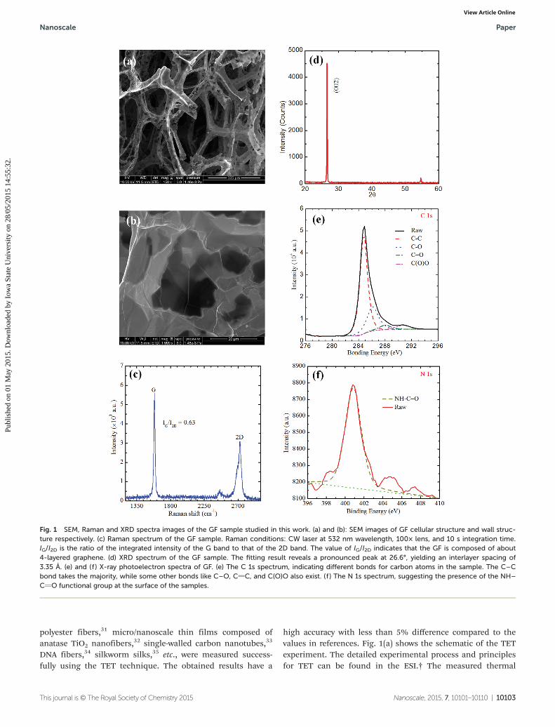
The graphene foam (purchased from Advanced Chemical Sup-plier Material Company) was synthesized by the chemicalvapor deposition (CVD) method. Fig. 1(a) and (b) show theimages of GF samples under a scanning electron microscope(SEM) from low to high magnification, where 3D porous foam-like structure of GF can be clearly seen. Fig. 1(c) presents theRaman spectrum of the GF sample. The ratio of the integratedintensity of G band to that of 2D band (IG/I2D) is 0.63, indicat-ing that there are about 4 layers of graphene in our GFsample.28 The crystal structure was examined by X-ray diffrac-tion (XRD) analysis presented in Fig. 1(c) and (d). The fittingresults in an interlayer spacing of 3.35 Å, which is very close tothe reported value of 3.4 nm for bilayered and three-layeredgraphene.29 The XPS result shows that the GF is mainly com-posed of carbon (89%), oxygen (8.43%), nitrogen (0.43%), andsilicon (2.14%). Fig. 1(e) shows the C 1s spectrum of GF. The N1s is presented in Fig. 1(f ), indicating the presence of a smallamount of the NH–CvO functional group on the surface of GFsamples.30 Details of the structure characterization can befound in the ESI.†

The thermal diffusivity of GF samples at different tempera-tures was measured to study how the thermal diffusivity varieswith decreasing temperature. A Janis closed cycle refrigerator(CCR) system is employed to provide a stable and reliableenvironmental temperature from 295 K to 10 K. The transientelectro-thermal (TET) technique developed by our laboratory isused in the experiment. The TET technique has been proven tobe an accurate and reliable approach to measuring thethermal diffusivity of various solid materials, including con-ductive, semi-conductive or nonconductive materials. Thethermal diffusivity of different materials, such as micro-scale

Paper Nanoscale

10102 | Nanoscale, 2015, 7, 10101–10110 This journal is © The Royal Society of Chemistry 2015

Publ

ishe

d on

01

May

201

5. D

ownl

oade

d by

Iow

a St

ate

Uni

vers

ity o

n 28

/05/

2015

14:

55:3

2.

View Article Online

polyester fibers,31 micro/nanoscale thin films composed ofanatase TiO2 nanofibers,32 single-walled carbon nanotubes,33

DNA fibers,34 silkworm silks,35 etc., were measured success-fully using the TET technique. The obtained results have a

high accuracy with less than 5% difference compared to thevalues in references. Fig. 1(a) shows the schematic of the TETexperiment. The detailed experimental process and principlesfor TET can be found in the ESI.† The measured thermal

Fig. 1 SEM, Raman and XRD spectra images of the GF sample studied in this work. (a) and (b): SEM images of GF cellular structure and wall struc-ture respectively. (c) Raman spectrum of the GF sample. Raman conditions: CW laser at 532 nm wavelength, 100× lens, and 10 s integration time.IG/I2D is the ratio of the integrated intensity of the G band to that of the 2D band. The value of IG/I2D indicates that the GF is composed of about4-layered graphene. (d) XRD spectrum of the GF sample. The fitting result reveals a pronounced peak at 26.6°, yielding an interlayer spacing of3.35 Å. (e) and (f ) X-ray photoelectron spectra of GF. (e) The C 1s spectrum, indicating different bonds for carbon atoms in the sample. The C–Cbond takes the majority, while some other bonds like C–O, CvC, and C(O)O also exist. (f ) The N 1s spectrum, suggesting the presence of the NH–CvO functional group at the surface of the samples.

Nanoscale Paper

This journal is © The Royal Society of Chemistry 2015 Nanoscale, 2015, 7, 10101–10110 | 10103

Publ

ishe

d on

01

May

201

5. D

ownl

oade

d by

Iow

a St

ate

Uni

vers

ity o

n 28

/05/

2015

14:

55:3

2.

View Article Online

diffusivity from TET is a combination of the real thermal diffu-sivity and the radiation effect:

αmeasure ¼ αþ 1ρcp

8εrσT03

DL2

π2; ð1Þ

where αmeasure is the measured thermal diffusivity, and α is thereal thermal diffusivity of GF. εr is the effective heat emissivityof GF, and σ = 5.67 × 10−8 W m−2 K−4 is the Stefan–Boltzmannconstant. D and L are the thickness and length of the sample,respectively. T0 is the environmental temperature and ρcp isthe specific heat of graphene foam per unit volume.

TET measurements were conducted at every 25 K ofenvironmental temperature from 295 K to 100 K. Denser datapoints are collected at low temperatures (<100 K) to have aclearer view of low temperature effects. After that, the sampleis taken out and cut shorter for the next experiment. Experi-

ments are repeated with the same sample with three differentlengths. The measured samples are detailed in Table 1. Thevoltage evolution (Vexp) was recorded using an oscilloscope(Tektronix DPO 3052 Digital Phosphor Oscilloscope). As azero-gap semiconductor, graphene’s resistance is inverselyproportional to its increasing temperature, which shouldbe linearly reflected in the decreasing voltage in our TETmeasurement. The inset in Fig. 2(b) shows the resistanceagainst temperature profile for sample 1 from 295 K to 10 K,

Table 1 Details of GF samples characterized in this work

Sample Sample_1 Sample_2 Sample_3

Length (mm) 5.14 3.74 1.01Width (mm) 1.37 1.38 1.37

Fig. 2 (a) Schematic of the experimental setup and data collection for the TET technique. The GF sample is suspended between two gold-coatedsilicon electrodes and compressed tightly by two smooth silicon wafers. The whole sample base is mounted on the cold head of the CCR system. Acurrent source supplies the step current and an oscilloscope records the voltage evolution for the GF sample. (b) The raw voltage against time datacollected by the oscilloscope for sample 1 at the environmental temperature of 195 K. The inset demonstrates the linear relationship between resist-ance and temperature for sample 1 from 295 K to 10 K. (c) Microscopy image of the GF sample (sample 1) suspended between two gold-coatedsilicon electrodes. (d) Theoretical fitting of the normalized temperature rise for sample 1 at different environmental temperatures: 295 K, 195 K, and10 K. Dots represent the experimental data and solid lines show the fitting result. These experiments are conducted in a vacuum lower than0.5 mTorr. The time for reaching the steady state in TET measurements becomes shorter and shorter as T0 decreases from 295 K to 10 K, demon-strating that the measured thermal diffusivity increases with decreasing temperature.

Paper Nanoscale

10104 | Nanoscale, 2015, 7, 10101–10110 This journal is © The Royal Society of Chemistry 2015

Publ

ishe

d on

01

May

201

5. D

ownl

oade

d by

Iow

a St

ate

Uni

vers

ity o

n 28

/05/

2015

14:

55:3

2.

View Article Online

which confirms the linear R–T relationship. A linear fitting canbe used to describe the R–T relationship: R = 26.85–0.0196 × T.Fig. 2(b) shows one of the voltage evolutions (sample 1 at195 K). The voltage before electrical heating is 1.104 V. Uponthe step current, the voltage begins to decrease and finallyreaches a steady voltage at about 1.091 V, resulting in thevoltage change of 1.18%. Given that the step current for thismeasurement is 47.2 mA, the resistance can be calculated as23.39 Ω and 23.11 Ω before and after the heating respectively.Based on the linear R–T relationship of sample 1, the tempera-ture increase is determined as 14.29 K. The recorded experi-mental V–t data are theoretically fitted using different trialvalues of the thermal diffusivity subsequently. Using eqn (2) inthe ESI† and MATLAB programming, the experimental dataare fitted by comparing with the theoretical curve withdifferent trial values of measured thermal diffusivity (αmeasure).Applying the least squares fitting technique, the value givingthe best fit of Vexp is taken as αmeasure. The αmeasure representsthe thermal diffusivity during the joule heating process. Thecorresponding real temperature can be approximated by theaverage of the environmental temperature (T0) and the stabletemperature of the sample (T1). Here, the real temperature (T )is taken as 195 + 14.29/2 ≈ 202 K. To determine the uncertaintyof the fittings, different trial values are also used for thefitting. It is found that when the trial values are changedby ±10%, the fitting curve obviously deviates from theexperimental data. Thus the fitting uncertainty was estimatedas 10%, but the real error should be much smaller since wemeasured each value of thermal diffusivity 30 times and tookthe average value as the final thermal diffusivity. In thisexample, αmeasure is determined as 2.38 × 10−4 m2 s−1 at thereal temperature of 202 K. The normalized temperature risecan be obtained using T* = [V(t ) − V0]/[V(t → ∞) − V0]. Fig. 2(d)shows the normalized temperature rise for sample 1 atdifferent environmental temperatures: 295 K, 195 K, and 10 K.As illustrated in the figure, the time for reaching the stabilitybecomes shorter and shorter as T0 decreases from 295 K to10 K, indicating that the measured thermal diffusivity isincreasing with decreasing temperature.

3. Thermal properties and defectlevel3.1. Thermal diffusivity of graphene foam and its variationagainst T

The result for αmeasure of the three samples against real temp-erature T [=(T0 + T1)/2] is summarized in Fig. 3. Here, αmeasure

is still a combination of the real thermal diffusivity (αreal) andthe radiation effect. The GF samples are cut from an equal-thickness GF film. From Table 1, the widths of the threesamples are almost equal with an error of less than 0.8%. Thelengths and widths were measured with INFINITY ANALYZEunder the microscope with a high accuracy. From eqn (1), wecan express αmeasure as: αmeasure = α + 8εrσT0

3L2/ρcpDπ2. Assum-ing uniform density, emissivity and αreal for the three samples,

which is reasonable considering that they are actually thesample with different lengths, the radiation effect should belinearly related to its length square L2. We plot the αmeasure–L

2

of the three samples at each temperature (see Fig. 3 inset forexample). αreal is then obtained by linear fitting and extra-polating to the point of L2 = 0. The real thermal diffusivity isalso plotted in Fig. 3.

αreal shows an increasing behavior as T goes down from299 K to 104 K. Below 104 K, αreal tends to be stable with aslight decrease from 43 K to 17 K. From the Wiedemann–Franzlaw, the contribution of electron transport to the thermal con-ductivity of graphene is negligible. The thermal behavior ofgraphene is governed by propagating phonons in the graphenelattice. The thermal transport ability of graphene is limited byphonon scattering in several mechanisms, mainly includingUmklapp phonon–phonon scattering (U-scattering), phonon-defect scattering and phonon-boundary scattering. Onlyphonons with wave vectors (kp) of the order of G/2 (G is thereciprocal lattice vector of the first Brillouin zone) participatein the U-scattering by collision. At near RT, the phonon energyis so high that almost all phonons possess high enough kp toparticipate in the thermal transfer. Thus U-scattering domi-nates the scattering process at near RT. As T goes down, latticeelastic vibrations in graphene weaken and phonon populationdecreases. The U-scattering weakens correspondingly, which

Fig. 3 The measured thermal diffusivity αmeasure against temperature Tfor the three GF samples and the resulting real thermal diffusivity of GF(αreal). αreal follows a linear increase with decreasing temperature from299 K to 104 K. At 104 K, αreal tends to be stable with a slight decreasefrom 43 K to 17 K. The top right inset is the measured thermal diffusivityagainst length square (L2) for the three GF samples at a temperature of54 K, showing one of the fitting process for determining the realthermal diffusivity of the sample. Triangles are for the experimental data,and the solid line represents the linear fitting.

Nanoscale Paper

This journal is © The Royal Society of Chemistry 2015 Nanoscale, 2015, 7, 10101–10110 | 10105

Publ

ishe

d on

01

May

201

5. D

ownl

oade

d by

Iow

a St

ate

Uni

vers

ity o

n 28

/05/

2015

14:

55:3

2.

View Article Online

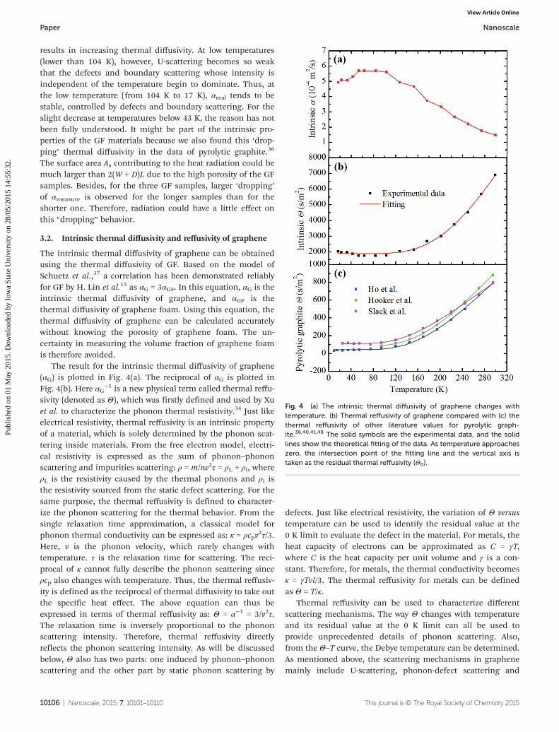
results in increasing thermal diffusivity. At low temperatures(lower than 104 K), however, U-scattering becomes so weakthat the defects and boundary scattering whose intensity isindependent of the temperature begin to dominate. Thus, atthe low temperature (from 104 K to 17 K), αreal tends to bestable, controlled by defects and boundary scattering. For theslight decrease at temperatures below 43 K, the reason has notbeen fully understood. It might be part of the intrinsic pro-perties of the GF materials because we also found this ‘drop-ping’ thermal diffusivity in the data of pyrolytic graphite.36

The surface area As contributing to the heat radiation could bemuch larger than 2(W + D)L due to the high porosity of the GFsamples. Besides, for the three GF samples, larger ‘dropping’of αmeasure is observed for the longer samples than for theshorter one. Therefore, radiation could have a little effect onthis “dropping” behavior.

3.2. Intrinsic thermal diffusivity and reffusivity of graphene

The intrinsic thermal diffusivity of graphene can be obtainedusing the thermal diffusivity of GF. Based on the model ofSchuetz et al.,37 a correlation has been demonstrated reliablyfor GF by H. Lin et al.15 as αG = 3αGF. In this equation, αG is theintrinsic thermal diffusivity of graphene, and αGF is thethermal diffusivity of graphene foam. Using this equation, thethermal diffusivity of graphene can be calculated accuratelywithout knowing the porosity of graphene foam. The un-certainty in measuring the volume fraction of graphene foamis therefore avoided.

The result for the intrinsic thermal diffusivity of graphene(αG) is plotted in Fig. 4(a). The reciprocal of αG is plotted inFig. 4(b). Here αG

−1 is a new physical term called thermal reffu-sivity (denoted as Θ), which was firstly defined and used by Xuet al. to characterize the phonon thermal resistivity.34 Just likeelectrical resistivity, thermal reffusivity is an intrinsic propertyof a material, which is solely determined by the phonon scat-tering inside materials. From the free electron model, electri-cal resistivity is expressed as the sum of phonon–phononscattering and impurities scattering: ρ = m/ne2τ = ρL + ρi, whereρL is the resistivity caused by the thermal phonons and ρi isthe resistivity sourced from the static defect scattering. For thesame purpose, the thermal reffusivity is defined to character-ize the phonon scattering for the thermal behavior. From thesingle relaxation time approximation, a classical model forphonon thermal conductivity can be expressed as: κ = ρcpv

2τ/3.Here, v is the phonon velocity, which rarely changes withtemperature. τ is the relaxation time for scattering. The reci-procal of κ cannot fully describe the phonon scattering sinceρcp also changes with temperature. Thus, the thermal reffusiv-ity is defined as the reciprocal of thermal diffusivity to take outthe specific heat effect. The above equation can thus beexpressed in terms of thermal reffusivity as: Θ = α−1 = 3/v2τ.The relaxation time is inversely proportional to the phononscattering intensity. Therefore, thermal reffusivity directlyreflects the phonon scattering intensity. As will be discussedbelow, Θ also has two parts: one induced by phonon–phononscattering and the other part by static phonon scattering by

defects. Just like electrical resistivity, the variation of Θ versustemperature can be used to identify the residual value at the0 K limit to evaluate the defect in the material. For metals, theheat capacity of electrons can be approximated as C = γT,where C is the heat capacity per unit volume and γ is a con-stant. Therefore, for metals, the thermal conductivity becomesκ = γTvl/3. The thermal reffusivity for metals can be definedas Θ = T/κ.

Thermal reffusivity can be used to characterize differentscattering mechanisms. The way Θ changes with temperatureand its residual value at the 0 K limit can all be used toprovide unprecedented details of phonon scattering. Also,from the Θ–T curve, the Debye temperature can be determined.As mentioned above, the scattering mechanisms in graphenemainly include U-scattering, phonon-defect scattering and

Fig. 4 (a) The intrinsic thermal diffusivity of graphene changes withtemperature. (b) Thermal reffusivity of graphene compared with (c) thethermal reffusivity of other literature values for pyrolytic graph-ite.36,40,41,48 The solid symbols are the experimental data, and the solidlines show the theoretical fitting of the data. As temperature approacheszero, the intersection point of the fitting line and the vertical axis istaken as the residual thermal reffusivity (Θ0).

Paper Nanoscale

10106 | Nanoscale, 2015, 7, 10101–10110 This journal is © The Royal Society of Chemistry 2015

Publ

ishe

d on

01

May

201

5. D

ownl

oade

d by

Iow

a St

ate

Uni

vers

ity o

n 28

/05/

2015

14:

55:3

2.

View Article Online

phonon-boundary scattering. According to Matthiessen’s rule,it is generally a good approximation to linearly add all the scat-tering effects for the overall scattering effect:

1τc

¼ 1τu

þ 1τdefects

þ 1τboundary

ð2Þ

For U-scattering, lattice elastic vibration weakens as thetemperature decreases, resulting in reduced U-scattering andincreased relaxation time τu. Thus, as the temperatureapproaches 0 K, the overall reversed relaxation time (1/τc)slowly reaches 1/τdefects + 1/τboundary. Thus Θ decreases to a con-stant: Θ(T →0) = 3/[v2(τdefect + τboundary)], which correspond-ingly reflects the defect and boundary scattering effects in thethermal reffusivity. It is defined as the residual thermal reffu-sivity (Θ0). For rare-defect crystallite materials, with no defectsand boundary scattering existing, Θ is expected to be zero atthe 0 K limit. To demonstrate this theory, we have studiedsome near-perfect materials in our previous work, for example,silicon, germanium, NaCl and NaF. When the temperaturegoes down to 0 K, their Θ truly decreases to zero just as thetheory predicts.34

Fig. 4(b) shows the profile of the intrinsic thermal reffusiv-ity of graphene varying with temperature. Clearly, Θ decreasesas the temperature decreases from 299 K to 100 K. When T isbelow 100 K, Θ gradually becomes stable and comes to Θ0. Tocompensate for the data fluctuation at low temperatures andreduce the error, the experimental data are fitted by a modelof phonon-scattering. From solid state physics, the phononpopulation of U-scattering follows a behavior of e−θ/2T at lowtemperatures,38 where θ is the Debye temperature of gra-phene. Our experiments are conducted at temperatures muchlower than θ (around 2000 K39). Combined with the residualthermal reffusivity theory, the model for thermal reffusivity isexpressed as Θ = Θ0 + C × e−θ/2T, where C is a constant. UsingOriginPro, the nonlinear curve fitting based on this equationfor GF is Θ = 1878 + 1.03 × 105 × e−906.6×T. Θ0 is accordinglydetermined as 1878 s m−2 and θ is 1813 ± 48 K. For our gra-phene foam sample, the residual thermal reffusivity Θ0 =1878 s m−2, taking about 27.2% of the RT reffusivity. Thefitting is also plotted in Fig. 4(b) with the experimental data.The fitting line shows excellent agreement with the data,demonstrating the U-scattering effect on the thermal trans-port. Our resulting Debye temperature is 1813 K. Althoughmany theoretical analyses suggested that the flexural acoustic(ZA) phonons provide the dominant contribution to thethermal transfer in graphene,20 our value is very close to theaverage θ (=1911 K) of the three acoustic modes in graphene,which is 2840 K for longitudinal mode (LA), 1775 K for trans-verse mode (TA) and 1120 K for ZA.20 This could result fromthe effect of the functional groups and other elements in GFas observed in XPS, which interrupt the phonon propagationand increase the energy coupling among ZA, LA and TAmodes.

To further demonstrate our residual thermal reffusivitytheory in graphene, we calculate the Θ evolution using some

experimental data of pyrolytic graphite in the litera-ture36,40,41,48 and fit these data using our thermal reffusivitymodel Θ = Θ0 + C × e−θ/2T. The results are presented in Fig. 4(c)for comparison. As seen from Fig. 4(c), the model gives excel-lent fittings for the three data groups. All the three groups of Θexperience the same decreasing pattern as the temperaturegoes down. Finally they reach each Θ0 value, which is deter-mined by the different defect level in their samples. For thedata from Ho et al.,40 Hooker et al.48 and Slack et al.,36 theresulting residual thermal reffusivity Θ0 are 43.3, 84.7 and112.1 s m−2 respectively. Considering that their Θ at roomtemperature are 795.4 s m−2, 881.8 s m−2 and 800.0 s m−2

respectively, the residual Θ0 takes only about 5%, 9.6% and14% of the whole reffusivity at room temperature. Theseresults indicate the highly oriented graphene layers and lowdefect structure in those pyrolytic graphite samples. TheirDebye temperatures are estimated as 1349 K, 1381 K and1133 K respectively. Their estimated Debye temperatures arevery close to the value of the ZA mode (1120 K), reflecting thedominance of the ZA mode phonon in heat conduction.

With the knowledge of Θ0, the mean free path of phonons(ls) induced by boundary and defect scattering can be esti-mated. ls represents the average distance that a phonontravels between two scatterings. When the temperatureapproaches 0 K, U-scattering gradually vanishes, and theremaining scattering mechanisms are primarily boundaryand defect scattering. When the temperature approachesabsolute zero, the residual thermal reffusivity can be writtenas Θ0 = 3/v2(τdefect + τboundary) = 3/vls under single relaxationtime approximation. To calculate the phonon velocity, thephonon dispersion relation of graphite given by Wirtz et al.42

is used. Phonon velocity is estimated as 9171 m s−1, which isthe average of the three branches: out-of-plane acoustic (ZA),longitudinal acoustic (LA), and transverse acoustic (TA). As aresult, ls from our data is estimated as 166 nm, which shouldbe smaller than the crystallite sizes of GF. For some rare-defect materials, such as silicon and NaCl, the point defectscattering can be rather small. Their crystallite sizes can beestimated by ls precisely using this method. For the pyrolyticgraphite sample, the corresponding mean free paths fromdefect and boundary scattering are determined as 7.56 μm,3.86 μm, and 2.92 μm for the data from Ho et al., Hookeret al. and Slack et al., respectively, which are close to thereported a-direction crystallite size of pyrolytic graphite.43

These result further indicate the low defect level in the pyro-lytic graphite samples.

3.3. Ideal thermal conductivity of graphene

By subtracting Θ0 from Θ, the ideal thermal diffusivity isobtained by αideal = 1/(Θ − Θ0). To reduce the error of data, weuse the fitting data as Θ. Using αideal and the specific heatcapacity of graphene, the ideal thermal conductivity of gra-phene can be determined as κideal = ρcpαideal, in which ρcp isthe volumetric specific heat of graphene. The literaturethermal conductivity of graphene ranges from dozens to thou-sands of W m−1 K−1 due to the different defect levels in each

Nanoscale Paper

This journal is © The Royal Society of Chemistry 2015 Nanoscale, 2015, 7, 10101–10110 | 10107

Publ

ishe

d on

01

May

201

5. D

ownl

oade

d by

Iow

a St

ate

Uni

vers

ity o

n 28

/05/

2015

14:

55:3

2.

View Article Online

graphene sample. Using our method, the difficulties formeasuring the defects levels in graphene samples can beaverted. Instead, the defect effect can be identified by Θ0.Fig. 5(a) shows the obtained ideal thermal diffusivity of gra-phene. αideal clearly has an eθ/2T dependence, suggesting thedominating Umklapp phonon scattering mechanism.

By multiplying ρcp, we are able to calculate κideal. As far aswe know, there has not been any experimental data for thespecific heat of graphene at low temperatures. In the tempera-ture range of 10 K to 300 K, the specific heat of graphite is nor-mally taken as that of graphene. Fig. 5(b) presents themeasured heat capacity of graphite by Desorbo et al.,44 whichis used here to calculate κideal. Fig. 5(c) shows κideal varyingwith temperature. At RT, κideal is about 300 W m−1 K−1. Thisvalue is much smaller than the previously reported thermalconductivity of 1500–5000 W m−1 K−1 for suspended gra-

phene.45 The difference might result from the curvatures andfolds of graphene planes inside the GF sample as seen in SEMimages [Fig. 1(b)], which largely increases the phonon scatter-ing. In addition, there are other chemical elements (N, O, Hand Si) and the residual functional group on the surface of theGF samples from the XPS results. For our GF, oxygen takesabout 8.43% in the sample. It has been reported by Mu et al.that oxygen coverage of 5% reduced the graphene thermal con-ductivity by 90%.46 These extra atoms inevitably distort theorder of the lattice so as to interrupt the phonon propagationin graphene planes and even impede the neighboring planes.As the temperature goes down, κideal increases all the way to17 K, which further confirms the absence of the defect scatter-ing effect. For the literature reported thermal conductivity pro-files of graphene, their peaks occur at temperatures from100 K to near RT. The peak position was determined by thedefect level in graphene samples. It has been suggested that asthe perfection of the graphite samples is improved, the peak ofthermal conductivity shifts from RT to about 80 K.47 In ourresult, since the defect effect has been completely subtracted,αideal increases all the way as expected. Numerous studiessuggest that the specific heat of graphite follows the Debye T3

law at very low temperature (<10 K), and transforms to ∼T2 inthe intermediate temperature range (10–100 K). The thermaldiffusivity of graphene has a temperature dependence as αideal ∼eθ/2T. Therefore, the resulting thermal conductivity should havea behavior of κideal ∼ T2 × eθ/2T, where θ = 1813 K in our work.As the temperature goes down from 300 K to 10 K, e1813/2T

increases faster than the decreasing rate of T2. Accordingly,κideal increases with decreasing temperature all the way. Theideal thermal conductivity of pyrolytic graphite was also calcu-lated from the literature data using our model. It can be seenfrom Fig. 5(c) that κideal of the three pyrolytic graphite followthe same pattern as the temperature goes down.

Our κideal value is smaller than that of pyrolytic graphite atnear RT (100–299 K), while it exceeds the value of pyrolyticgraphite below 100 K. This demonstrates the superior thermalconductivity of graphene compared with pyrolytic graphite. Asthe temperature goes down, κideal increases rapidly and goesbeyond 105 W m−1 K−1 below 80 K based on our calculations.The data below 80 K should be used with less confidence sincethe specific heat values are taken from graphite experiments,which may be higher than the real specific heat of graphene.14

In addition, the error of fitted thermal reffusivity is larger atlow temperatures due to the data perturbation at low tempera-tures, which results in the larger error in the value of idealthermal diffusivity. In this work, the low temperature range ischosen in order to identify the defect level of graphene foam.These results illustrate the phonon scattering mechanism ingraphene at low temperatures and shed light on understand-ing the thermal behavior of graphene-based materials againsttemperature variation. The ideal thermal conductivity of gra-phene and the corresponding scattering mechanisms at hightemperatures (room temperature to 1000 °C) will be furtherinvestigated in the near future once our new high-temperaturevacuum stage is ready to use.

Fig. 5 (a) The ideal thermal diffusivity of graphene. (b) The experimentaldata for specific heat of graphite.44 (c) The ideal thermal conductivity ofgraphene (κideal) against temperature compared with what we obtainedfrom other literature data of pyrolytic graphite.36,40,41,48 The data insidethe orange rectangle (below 80 K) are less reliable due to the error of αGat low temperatures and the undecided difference of specific heatbetween graphene and graphite.

Paper Nanoscale

10108 | Nanoscale, 2015, 7, 10101–10110 This journal is © The Royal Society of Chemistry 2015

Publ

ishe

d on

01

May

201

5. D

ownl

oade

d by

Iow

a St

ate

Uni

vers

ity o

n 28

/05/

2015

14:

55:3

2.

View Article Online

4. Conclusion

This work investigated the thermal transport in graphenefoam from RT to 17 K using the TET technique. The three-dimensional interconnected foam-like samples basicallyconsist of four-layered graphene. The XPS result uncovers thechemical composition of carbon (89%), oxygen (8.43%), nitro-gen (0.43%), and silicon (2.14%). The N 1s spectrum indicatesthe presence of a small amount of NH–CvO functional groupon the surface of the GF sample. The intrinsic thermal diffu-sivity (αG) of graphene is accurately determined after subtract-ing the radiation effect. We identified the defect-inducedphonon scattering effects in thermal transport of graphene byfitting the thermal reffusivity Θ to the point of T = 0 K. Usingthe residual thermal reffusivity (Θ0), we are able to evaluate theDebye temperature and the defect-phonon scattering meanfree path of graphene. Θ0 is found to be 1878 s m−2 for thestudied graphene foam, and 43–112 s m−2 for three highlycrystalline graphite materials. This indicates the orders ofmagnitude higher defect level in the GF. The defect-inducedphonon scattering gave a long mean free path of 166 nm. TheDebye temperature of graphene was determined at 1813 K,agreeing well with the average theoretical Debye temperature(1911 K) of TA, ZA, and LA phonons in graphene. By subtract-ing the residual thermal reffusivity, we obtained the idealthermal diffusivity and conductivity of the studied graphene.The ideal thermal conductivity (κideal) resulting from Umklappphonon–phonon scattering was found to increase all theway up with decreasing temperature. At RT, κideal is around300 W m−1 K−1. It could go up to greater than 105 W m−1 K−1

when the temperature goes down to 80 K. The ideal thermalconductivity of several reference graphite samples shows asimilar trend and comparable results.

Acknowledgements

Army Research Office (W911NF-12-1-0272), Office of NavalResearch (N000141210603), and National Science Foundation(CBET1235852, CMMI1264399, and CMMI1200397) are grate-fully acknowledged for support of this work. X.W. acknowl-edges the partial support from the “Eastern Scholar” Programof Shanghai, China. Y.X is supported by the China ScholarshipCouncil.

Notes and references

1 M. A. Worsley, P. J. Pauzauskie, T. Y. Olson, J. Biener,J. H. Satcher and T. F. Baumann, J. Am. Chem. Soc., 2010,132, 14067–14069.

2 A. A. Balandin, S. Ghosh, W. Z. Bao, I. Calizo,D. Teweldebrhan, F. Miao and C. N. Lau, Nano Lett., 2008,8, 902–907.

3 H. Y. Sun, Z. Xu and C. Gao, Adv. Mater., 2013, 25, 2554–2560.

4 C. Wang, L. Zhang, Z. H. Guo, J. G. Xu, H. Y. Wang,K. F. Zhai and X. Zhuo, Microchim. Acta, 2010, 169,1–6.

5 F. Bonaccorso, Z. Sun, T. Hasan and A. C. Ferrari, Nat.Photonics, 2010, 4, 611–622.

6 S. Ghosh, I. Calizo, D. Teweldebrhan, E. P. Pokatilov,D. L. Nika, A. A. Balandin, W. Bao, F. Miao and C. N. Lau,Appl. Phys. Lett., 2008, 92, 151911–151911.

7 X. Wang, L. J. Zhi and K. Mullen, Nano Lett., 2008, 8, 323–327.

8 H. L. Wang, L. F. Cui, Y. A. Yang, H. S. Casalongue,J. T. Robinson, Y. Y. Liang, Y. Cui and H. J. Dai, J. Am.Chem. Soc., 2010, 132, 13978–13980.

9 D. Cohen-Tanugi and J. C. Grossman, Nano Lett., 2012, 12,3602–3608.

10 X. M. Sun, Z. Liu, K. Welsher, J. T. Robinson, A. Goodwin,S. Zaric and H. J. Dai, Nano Res., 2008, 1, 203–212.

11 S. S. Chen, Q. Z. Wu, C. Mishra, J. Y. Kang, H. J. Zhang,K. J. Cho, W. W. Cai, A. A. Balandin and R. S. Ruoff, Nat.Mater., 2012, 11, 203–207.

12 J. U. Lee, D. Yoon, H. Kim, S. W. Lee and H. Cheong, Phys.Rev. B: Condens. Matter, 2011, 83, 081419.

13 C. Faugeras, B. Faugeras, M. Orlita, M. Potemski, R. R. Nairand A. K. Geim, ACS Nano, 2010, 4, 1889–1892.

14 E. Pop, V. Varshney and A. K. Roy, MRS Bull., 2012, 37,1273–1281.

15 H. Lin, S. Xu, X. W. Wang and N. Mei, Nanotechnology,2013, 24, 415706.

16 W. W. Cai, A. L. Moore, Y. W. Zhu, X. S. Li, S. S. Chen,L. Shi and R. S. Ruoff, Nano Lett., 2010, 10, 1645–1651.

17 J. H. Chen, C. Jang, S. Adam, M. S. Fuhrer, E. D. Williamsand M. Ishigami, Nat. Phys., 2008, 4, 377–381.

18 H. C. Schniepp, J. L. Li, M. J. McAllister, H. Sai, M. Herrera-Alonso, D. H. Adamson, R. K. Prud’homme, R. Car,D. A. Saville and I. A. Aksay, J. Phys. Chem. B, 2006, 110,8535–8539.

19 D. L. Nika, E. P. Pokatilov, A. S. Askerov and A. A. Balandin,Phys. Rev. B: Condens. Matter, 2009, 79, 155413.

20 J. C. Zhang, X. P. Huang, Y. N. Yue, J. M. Wang andX. W. Wang, Phys. Rev. B: Condens. Matter, 2011, 84,235416.

21 W. J. Evans, L. Hu and P. Keblinski, Appl. Phys. Lett., 2010,96, 203112.

22 L. Lindsay, D. A. Broido and N. Mingo, Phys. Rev. B:Condens. Matter, 2010, 82, 161402.

23 E. Munoz, J. X. Lu and B. I. Yakobson, Nano Lett., 2010, 10,1652–1656.

24 F. Yavari, Z. P. Chen, A. V. Thomas, W. C. Ren, H. M. Chengand N. Koratkar, Sci. Rep., 2011, 1, 166.

25 Y. Zhao, J. Liu, Y. Hu, H. H. Cheng, C. G. Hu, C. C. Jiang,L. Jiang, A. Y. Cao and L. T. Qu, Adv. Mater., 2013, 25, 591–595.

26 N. Li, Q. Zhang, S. Gao, Q. Song, R. Huang, L. Wang,L. W. Liu, J. W. Dai, M. L. Tang and G. S. Cheng, Sci. Rep.,2013, 3, 1604.

Nanoscale Paper

This journal is © The Royal Society of Chemistry 2015 Nanoscale, 2015, 7, 10101–10110 | 10109

Publ

ishe

d on

01

May

201

5. D

ownl

oade

d by

Iow

a St

ate

Uni

vers

ity o

n 28

/05/

2015

14:

55:3

2.

View Article Online

27 M. T. Pettes, H. X. Ji, R. S. Ruoff and L. Shi, Nano Lett.,2012, 12, 2959–2964.

28 D. Graf, F. Molitor, K. Ensslin, C. Stampfer, A. Jungen,C. Hierold and L. Wirtz, Nano Lett., 2007, 7, 238–242.

29 E. V. Castro, K. S. Novoselov, S. V. Morozov, N. M. R. Peres,J. M. B. L. Dos Santos, J. Nilsson, F. Guinea, A. K. Geim andA. H. Castro Neto, Phys. Rev. Lett., 2007, 99, 216802.

30 Z. Q. Luo, S. H. Lim, Z. Q. Tian, J. Z. Shang, L. F. Lai,B. MacDonald, C. Fu, Z. X. Shen, T. Yu and J. Y. Lin, J.Mater. Chem., 2011, 21, 8038–8044.

31 X. H. Feng and X. W. Wang, Thin Solid Films, 2011, 519,5700–5705.

32 X. Feng, X. Wang, X. Chen and Y. Yue, Acta Mater., 2011,59, 1934–1944.

33 J. Q. Guo, X. W. Wang and T. Wang, J. Appl. Phys., 2007,101, 063537.

34 Z. L. Xu, X. W. Wang and H. Q. Xie, Polymer, 2014, 55,6373–6380.

35 G. Q. Liu, X. P. Huang, Y. J. Wang, Y. Q. Zhang andX. W. Wang, Soft Matter, 2012, 8, 9792–9799.

36 G. A. Slack, Phys. Rev., 1962, 127, 694–701.37 M. A. Schuetz and L. R. Glicksman, J. Cell Plast., 1984, 20,

114–121.

38 C. Kittel and P. McEuen, Introduction to solid state physics,J. Wiley, Hoboken, NJ, 8th edn, 2005, p. 126.

39 L. A. Falkovsky, Phys. Rev. B: Condens. Matter, 2007, 75,033409.

40 C. Y. Ho, R. W. Powell and P. E. Liley, Thermal conductivityof the elements: a comprehensive review, American ChemicalSociety, Washington, 1975, p. 150.

41 S. S. Chen, A. L. Moore, W. W. Cai, J. W. Suk, J. H. An,C. Mishra, C. Amos, C. W. Magnuson, J. Y. Kang, L. Shi andR. S. Ruoff, ACS Nano, 2011, 5, 321–328.

42 L. Wirtz and A. Rubio, Solid State Commun., 2004, 131,141–152.

43 R. A. Morant, J. Phys. D: Appl. Phys., 1970, 3, 1367–1373.

44 W. Desorbo and W. W. Tyler, J. Chem. Phys., 1953, 21,1660–1663.

45 A. A. Balandin, Nat. Mater., 2011, 10, 569–581.46 X. Mu, X. F. Wu, T. Zhang, D. B. Go and T. F. Luo, Sci. Rep.,

2014, 4, 3909.47 J. W. Klett, A. D. McMillan, N. C. Gallego and C. A. Walls,

J. Mater. Sci., 2004, 39, 3659–3676.48 C. N. Hooker, A. R. Ubbelohd and D. A. Young, Proc. R. Soc.

London, Ser. A, 1965, 284, 17.

Paper Nanoscale

10110 | Nanoscale, 2015, 7, 10101–10110 This journal is © The Royal Society of Chemistry 2015

Publ

ishe

d on

01

May

201

5. D

ownl

oade

d by

Iow

a St

ate

Uni

vers

ity o

n 28

/05/

2015

14:

55:3

2.

View Article Online