The Deep Space Network Radio Astronomy UserGuide

March 9, 2020

Document Owner: Joseph Lazio (Jet Propulsion Laboratory, California Institute of Technology)c⃝2020. California Institute of Technology. Government sponsorship acknowledged.

Contents

Changes to this Document . . . . . . . . . . . . . . . . . . . . . . . . . . . . . . . . . . . . ivAcknowledgments . . . . . . . . . . . . . . . . . . . . . . . . . . . . . . . . . . . . . . . . . v

1 Introduction 1

2 Proposal Submission and DSN Scheduling 3

3 70 m Subnetwork 43.1 Antennas . . . . . . . . . . . . . . . . . . . . . . . . . . . . . . . . . . . . . . . . . . 43.2 Efficiency and Gain . . . . . . . . . . . . . . . . . . . . . . . . . . . . . . . . . . . . . 43.3 Resolution . . . . . . . . . . . . . . . . . . . . . . . . . . . . . . . . . . . . . . . . . . 5

4 34 m Subnetwork 74.1 Antennas . . . . . . . . . . . . . . . . . . . . . . . . . . . . . . . . . . . . . . . . . . 74.2 Efficiency and Gain . . . . . . . . . . . . . . . . . . . . . . . . . . . . . . . . . . . . . 84.3 Resolution . . . . . . . . . . . . . . . . . . . . . . . . . . . . . . . . . . . . . . . . . . 104.4 Polarization . . . . . . . . . . . . . . . . . . . . . . . . . . . . . . . . . . . . . . . . . 10

5 Receiving Systems 125.1 Radio Astronomical K Band (17 GHz–27 GHz) . . . . . . . . . . . . . . . . . . . . . 125.2 Radio Astronomical Q Band (38 GHz–50 GHz) . . . . . . . . . . . . . . . . . . . . . 135.3 L Band (1628 MHz–1708 MHz) . . . . . . . . . . . . . . . . . . . . . . . . . . . . . . 135.4 S Band (2200 MHz–2300 MHz) . . . . . . . . . . . . . . . . . . . . . . . . . . . . . . 135.5 X Band (8200 MHz–8600 MHz) . . . . . . . . . . . . . . . . . . . . . . . . . . . . . . 145.6 Spacecraft Tracking K Band (25.5 GHz–27 GHz) . . . . . . . . . . . . . . . . . . . . 145.7 Ka Band (31.8 GHz–32.3 GHz) . . . . . . . . . . . . . . . . . . . . . . . . . . . . . . 14

6 Signal Transport 18

7 Backends 217.1 Fast Fourier Transform Spectrometer (FFTS)-Madrid . . . . . . . . . . . . . . . . . 217.2 DSN Pulsar Processor-Canberra . . . . . . . . . . . . . . . . . . . . . . . . . . . . . 217.3 DSN Radio Astronomy Spectrometer-Canberra . . . . . . . . . . . . . . . . . . . . . 22

7.3.1 Level 0 Data . . . . . . . . . . . . . . . . . . . . . . . . . . . . . . . . . . . . 227.3.2 Level 1 Data . . . . . . . . . . . . . . . . . . . . . . . . . . . . . . . . . . . . 22

7.4 VLBI Radio Astronomy (VRA) Assembly . . . . . . . . . . . . . . . . . . . . . . . . 23

A Proposal Preparation and Observation Planning 24

i

List of Figures

1.1 The DSN radio antennas and locations. . . . . . . . . . . . . . . . . . . . . . . . . . 1

3.1 DSS-43, the 70 m antenna at the Canberra Complex . . . . . . . . . . . . . . . . . . 5

4.1 Illustration of key aspects of a DSN 34 m beam wave guide antenna . . . . . . . . . 8

5.1 Overview of the DSS-43 radio astronomical K-band system. . . . . . . . . . . . . . . 155.2 Low-noise assembly (“front-end”) for the DSS-43 K-band system . . . . . . . . . . . 165.3 Downconverter for the DSS-43 K-band system . . . . . . . . . . . . . . . . . . . . . . 17

6.1 Signal transport at the Canberra Deep Space Communications Complex . . . . . . . 196.2 Signal transport at the Madrid Deep Space Communications Complex . . . . . . . . 20

A.1 Visibility of sources from Canberra Deep Space Communications Complex . . . . . . 25A.2 Visibility of sources from the Madrid Deep Space Communications Complex . . . . . 26A.3 Visibility of sources from the Goldstone Deep Space Communications Complex . . . 27

ii

List of Tables

1.1 Deep Space Network Complexes . . . . . . . . . . . . . . . . . . . . . . . . . . . . . . 1

2.1 DSN Radio Astronomy proposal categories . . . . . . . . . . . . . . . . . . . . . . . 3

3.1 70 m Aperture Efficiencies and Gains . . . . . . . . . . . . . . . . . . . . . . . . . . . 63.2 70 m Antenna Beam Widths . . . . . . . . . . . . . . . . . . . . . . . . . . . . . . . 6

4.1 Future DSN 34 m Beam Wave Guide Antennas . . . . . . . . . . . . . . . . . . . . . 74.2 34 m Aperture Efficiencies and Gains . . . . . . . . . . . . . . . . . . . . . . . . . . . 94.3 34 m Antenna Beam Widths . . . . . . . . . . . . . . . . . . . . . . . . . . . . . . . 104.4 34 m Antenna Polarization Capabilities . . . . . . . . . . . . . . . . . . . . . . . . . 11

7.1 DSN Radio Astronomy Spectrometer modes . . . . . . . . . . . . . . . . . . . . . . . 22

iii

Changes to this Document

Revision Date Summary

Original 2020 March

iv

Acknowledgments

This document reflects the work and input of many individuals and builds upon a significant historyof radio astronomy within NASA’s Deep Space Network. Further, the radio astronomy activitieswithin the Deep Space Network would not be possible without the efforts of the many engineersand technicians, at all three Complexes, who maintain the antennas and related infrastructure andhave kept the Deep Space Network operating “around-the-clock” for over 50 years.

A likely incomplete list of those having provided notable efforts to DSN Radio Astronomyinclude

• Graham Baines (Canberra Deep Space Communications Complex)

• Alina Bedrossian (Jet Propulsion Laboratory, California Institute of Technology)

• Shinji Horiuchi (Canberra Deep Space Communications Complex)

• Thomas Kuiper (Jet Propulsion Laboratory, California Institute of Technology, retired)

• Danny Luong (Jet Propulsion Laboratory, California Institute of Technology)

• Luis Neira (Madrid Deep Space Communications Complex)

• Ricardo Rizzo (Centro de Astrobiologıa)

• Lawrence Teitelbaum (Jet Propulsion Laboratory, California Institute of Technology)

• Manuel Vazquez (Madrid Deep Space Communications Complex)

• Cristina Garcia-Miro

• Manuel Franco (deceased)

• Michael Klein (deceased)

We thank the authors of the Green Bank Telescope Proposal Guide and the Parkes RadioTelescope proposal guide for the guidance in producing this document.

This work was carried out at the Jet Propulsion Laboratory, California Institute of Technology,under a contract with the National Aeronautics and Space Administration (80NM0018D004).

v

Chapter 1

Introduction

The Deep Space Network (DSN) is the spacecraft tracking and communication infrastructure forNASA’s deep space missions. It consists of three sites, approximately equally separated in (terres-trial) longitude, with multiple radio antennas at each site. Table 1.1 summarizes the key charac-teristics of the three sites; Figure 1.1 illustrates the locations of the various sites.

Table 1.1: Deep Space Network ComplexesName Longitude Latitude Antennas

Goldstone 116◦ 46′ 44′′ W 35◦ 16′ 53′′ N DSS-14 (70 m), DSS-24, DSS-25, DSS-26 (34 m)Canberra 148◦ 58′ 56′′ E 35◦ 24′ 06′′ S DSS-43 (70 m), DSS-34, DSS-35, DSS-36 (34 m)Madrid 4◦ 14′ 59′′ W 40◦ 25′ 45′′ N DSS-63 (70 m), DSS-54, DSS-55 (34 m)

Figure 1.1: The DSN radio antennas and locations.

The DSN antennas have a long history of radio astronomical observations. Contributions ofDSN antennas to astronomical discoveries include the first identification of superluminal motion

1

(Cohen et al. 1971); demonstration of space-based very long baseline interferometry (VLBI) fromwhich a clear indication of violation of the inverse Compton limit and constraints on the physicalprocesses occurring in the central engines resulted (Levy et al. 1986, 1989; Linfield et al. 1989); thefirst detection of the infall and the inside-out collapse process during stellar formation (Velusamy,Kuiper, & Langer 1995; Kuiper et al. 1996); and demonstration of a continued gap in understandingof stellar structure and Galactic chemical evolution (the so-called “3He problem”) by detection ofa hyperfine line of 3He+ in the planetary nebula IC 418 (Guzman-Ramirez et al. 2016).

DSN antennas also have played an integral role in establishing and maintaining realizationsof the International Celestial Reference Frame (ICRF, Fey et al. 2015; Charlot et al. 2020). TheICRF is not only the defining frame used for specifying the coordinates of all astronomical sources,it serves as the reference against which the plane-of-sky positions of deep space spacecraft aredetermined for navigation of NASA’s deep space missions.

The focus of this document is on passive radio astronomical observations, of solar system objectsother than the Sun or of celestial sources beyond the solar system, and including astrometricobservations. Radar astronomy observations of solar system bodies is beyond the scope of thisdocument but is described by Dvorsky et al. (1992) and Slade et al. (2011) and references within.In a similar spirit, the transmit capabilities of the DSN antennas are not described here.

Much of this material is also presented in a series of documents contained in the DSN’s Telecom-munications Interfaces (2019), known colloquially as the 810-005 (with Modules 101, 104, and 211of most relevance to radio astronomical observations), but it is presented here in a manner that ismore common for radio astronomical observations.

2

Chapter 2

Proposal Submission and DSNScheduling

The DSN antennas can be used in a stand alone capacity or as part of a very long baseline inter-ferometry (VLBI) observation. Three important principles apply to all proposals to use the DSNfor radio astronomy:

• The prime responsibility of the DSN antennas is for spacecraft telemetry, tracking, and com-mand (TT&C). While every effort will be made to accommodate projects that require timecritical observations or observations at specific epochs, such observations can be challengingto schedule given the TT&C needs of the various missions that depend upon the DSN.

• The DSN schedules time four to six months in advance. While every effort will be made toaccommodate proposals submitted less than six months in advance, review and scheduling ofprojects will be facilitated by submission six months in advance.

• It is a basic requirement for all proposals to use one or more DSN antennas for radio astronomymust specify how the proposed observations require some unique capability of the DSN.

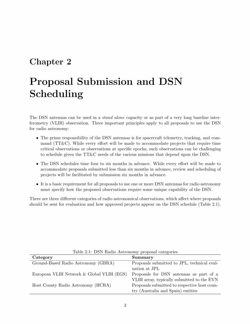
There are three different categories of radio astronomical observations, which affect where proposalsshould be sent for evaluation and how approved projects appear on the DSN schedule (Table 2.1).

Table 2.1: DSN Radio Astronomy proposal categoriesCategory Summary

Ground-Based Radio Astronomy (GBRA) Proposals submitted to JPL, technical eval-uation at JPL

European VLBI Network & Global VLBI (EGS) Proposals for DSN antennas as part of aVLBI array, typically submitted to the EVN

Host County Radio Astronomy (HCRA) Proposals submitted to respective host coun-try (Australia and Spain) entities

3

Chapter 3

70 m Subnetwork

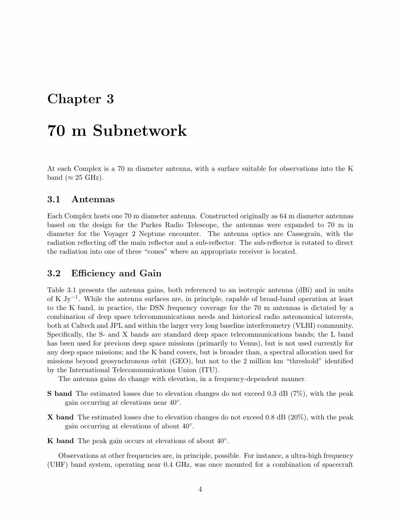
At each Complex is a 70 m diameter antenna, with a surface suitable for observations into the Kband (≈ 25 GHz).

3.1 Antennas

Each Complex hosts one 70 m diameter antenna. Constructed originally as 64 m diameter antennasbased on the design for the Parkes Radio Telescope, the antennas were expanded to 70 m indiameter for the Voyager 2 Neptune encounter. The antenna optics are Cassegrain, with theradiation reflecting off the main reflector and a sub-reflector. The sub-reflector is rotated to directthe radiation into one of three “cones” where an appropriate receiver is located.

3.2 Efficiency and Gain

Table 3.1 presents the antenna gains, both referenced to an isotropic antenna (dBi) and in unitsof K Jy−1. While the antenna surfaces are, in principle, capable of broad-band operation at leastto the K band, in practice, the DSN frequency coverage for the 70 m antennas is dictated by acombination of deep space telecommunications needs and historical radio astronomical interests,both at Caltech and JPL and within the larger very long baseline interferometry (VLBI) community.Specifically, the S- and X bands are standard deep space telecommunications bands; the L bandhas been used for previous deep space missions (primarily to Venus), but is not used currently forany deep space missions; and the K band covers, but is broader than, a spectral allocation used formissions beyond geosynchronous orbit (GEO), but not to the 2 million km “threshold” identifiedby the International Telecommunications Union (ITU).

The antenna gains do change with elevation, in a frequency-dependent manner.

S band The estimated losses due to elevation changes do not exceed 0.3 dB (7%), with the peakgain occurring at elevations near 40◦.

X band The estimated losses due to elevation changes do not exceed 0.8 dB (20%), with the peakgain occurring at elevations of about 40◦.

K band The peak gain occurs at elevations of about 40◦.

Observations at other frequencies are, in principle, possible. For instance, a ultra-high frequency(UHF) band system, operating near 0.4 GHz, was once mounted for a combination of spacecraft

4

Figure 3.1: DSS-43, the 70 m antenna at the Canberra Complex. Two of the three receiver cones arevisible below the subreflector; the third is hidden behind the two visible cones. (In the backgroundis a 34 m beam wave guide antenna.)

telecommunications and potential radio astronomical observations. Installation of systems at otherfrequencies can be considered; discussions with contacts identified earlier in this document (§2) areencouraged.

3.3 Resolution

The beamwidths of the antennas are well modeled by a symmetric function of θ = 16.2′(1GHz/ν),for a frequency in units of gigahertz, or θ = 0.54′(λ/1 cm). Table 3.2 summarizes the half-powerbeamwidth of the antennas for the specific operational frequencies.

5

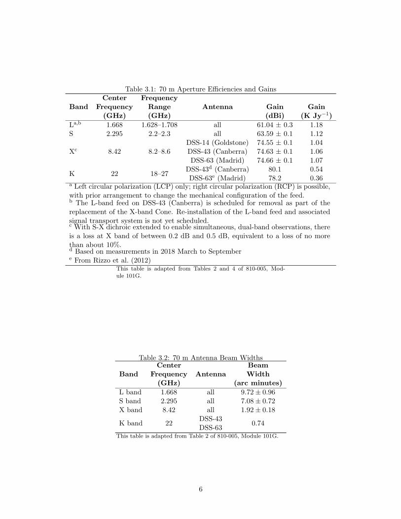
Table 3.1: 70 m Aperture Efficiencies and GainsCenter Frequency

Band Frequency Range Antenna Gain Gain(GHz) (GHz) (dBi) (K Jy−1)

La,b 1.668 1.628–1.708 all 61.04 ± 0.3 1.18S 2.295 2.2–2.3 all 63.59 ± 0.1 1.12

Xc 8.42 8.2–8.6DSS-14 (Goldstone) 74.55 ± 0.1 1.04DSS-43 (Canberra) 74.63 ± 0.1 1.06DSS-63 (Madrid) 74.66 ± 0.1 1.07

K 22 18–27DSS-43d (Canberra) 80.1 0.54DSS-63e (Madrid) 78.2 0.36

a Left circular polarization (LCP) only; right circular polarization (RCP) is possible,with prior arrangement to change the mechanical configuration of the feed.b The L-band feed on DSS-43 (Canberra) is scheduled for removal as part of thereplacement of the X-band Cone. Re-installation of the L-band feed and associatedsignal transport system is not yet scheduled.c With S-X dichroic extended to enable simultaneous, dual-band observations, thereis a loss at X band of between 0.2 dB and 0.5 dB, equivalent to a loss of no morethan about 10%.d Based on measurements in 2018 March to Septembere From Rizzo et al. (2012)

This table is adapted from Tables 2 and 4 of 810-005, Mod-ule 101G.

Table 3.2: 70 m Antenna Beam WidthsCenter Beam

Band Frequency Antenna Width(GHz) (arc minutes)

L band 1.668 all 9.72± 0.96S band 2.295 all 7.08± 0.72X band 8.42 all 1.92± 0.18

K band 22DSS-43

0.74DSS-63

This table is adapted from Table 2 of 810-005, Module 101G.

6

Chapter 4

34 m Subnetwork

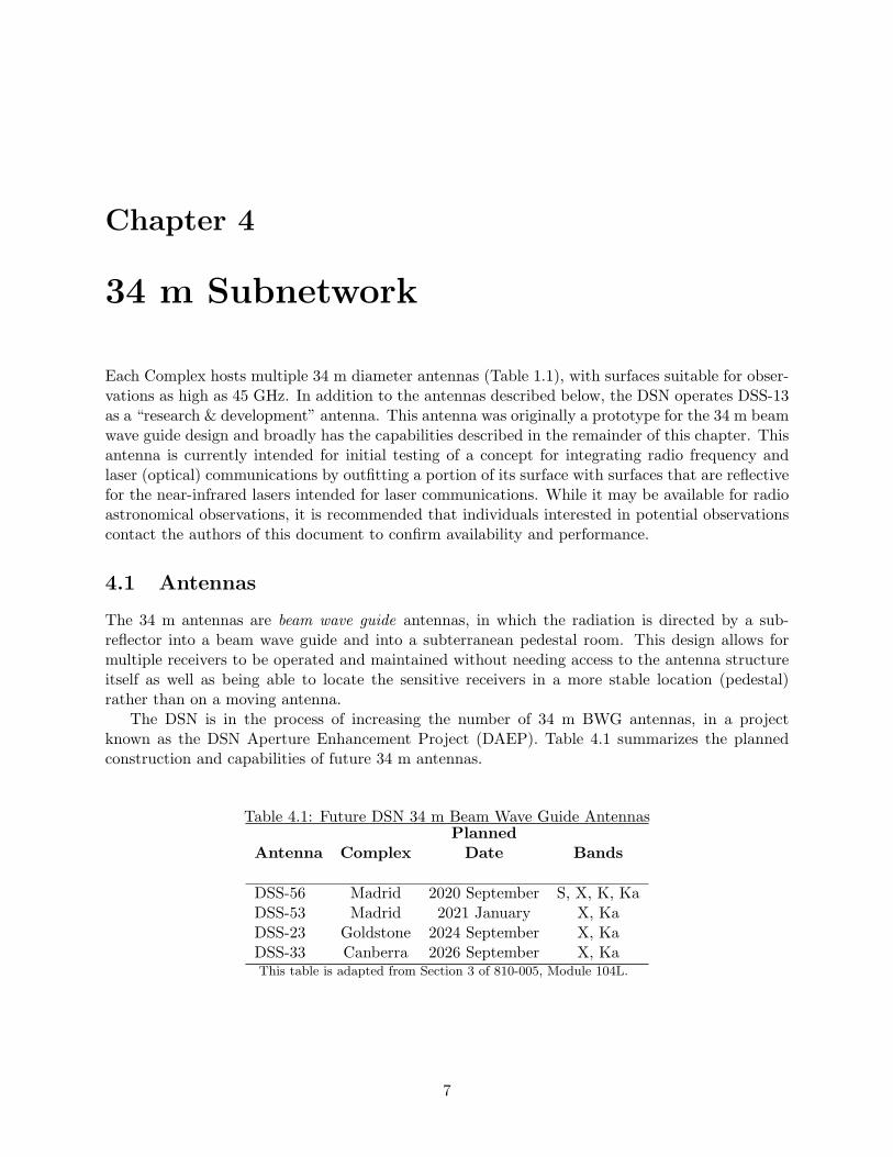
Each Complex hosts multiple 34 m diameter antennas (Table 1.1), with surfaces suitable for obser-vations as high as 45 GHz. In addition to the antennas described below, the DSN operates DSS-13as a “research & development” antenna. This antenna was originally a prototype for the 34 m beamwave guide design and broadly has the capabilities described in the remainder of this chapter. Thisantenna is currently intended for initial testing of a concept for integrating radio frequency andlaser (optical) communications by outfitting a portion of its surface with surfaces that are reflectivefor the near-infrared lasers intended for laser communications. While it may be available for radioastronomical observations, it is recommended that individuals interested in potential observationscontact the authors of this document to confirm availability and performance.

4.1 Antennas

The 34 m antennas are beam wave guide antennas, in which the radiation is directed by a sub-reflector into a beam wave guide and into a subterranean pedestal room. This design allows formultiple receivers to be operated and maintained without needing access to the antenna structureitself as well as being able to locate the sensitive receivers in a more stable location (pedestal)rather than on a moving antenna.

The DSN is in the process of increasing the number of 34 m BWG antennas, in a projectknown as the DSN Aperture Enhancement Project (DAEP). Table 4.1 summarizes the plannedconstruction and capabilities of future 34 m antennas.

Table 4.1: Future DSN 34 m Beam Wave Guide AntennasPlanned

Antenna Complex Date Bands

DSS-56 Madrid 2020 September S, X, K, KaDSS-53 Madrid 2021 January X, KaDSS-23 Goldstone 2024 September X, KaDSS-33 Canberra 2026 September X, KaThis table is adapted from Section 3 of 810-005, Module 104L.

7

Figure 4.1: (left) Illustration of key aspects of a DSN 34 m beam wave guide antenna. (FromImbriale 2003.) (right) DSS-36, the most recently constructed 34 m beam wave guide antenna inAustralia. The beam wave guide shroud is apparent behind the reflector.

4.2 Efficiency and Gain

Table 4.2 presents the antenna gains, both referenced to an isotropic antenna (dBi) and in unitsof K Jy−1. At present, the DSN frequency coverage for the 34 m antennas is dictated solely byspacecraft telecommunications needs, with the exception of DSS-54 at MDSCC, at which there isa radio astronomical Q band system installed (§5.2). Specifically, the S-, X-, and Ka bands arestandard deep space telecommunications bands; there is also a K band capability for “near Earth”telecommunications.1 Further, the frequency coverage is not uniform at all antennas, with someantennas having frequency capabilities that others do not.

These values do change with elevation, in a frequency-dependent manner.

S band The estimated losses due to elevation changes do not exceed 0.4 dB (10%), with the peakgain occurring at elevations near 40◦.

X band The estimated losses due to elevation changes do not exceed 0.6 dB (15%), with the peakgain occurring at elevations of about 50◦.

K band The estimated losses due to elevation changes do not exceed 1.2 dB (30%) under goodweather conditions but can approach 4 dB (over a factor of 2) under poor weather conditions.The peak gain occurs at elevations of about 50◦.

Ka band The estimated losses due to elevation changes do not exceed 2 dB (58%) under goodweather conditions but can approach 4 dB (over a factor of 2) under poor weather conditions.The peak gain occurs at elevations of about 50◦.

1The boundary between deep space and near-Earth is defined by the International Telecommunications Union as2 million km.

8

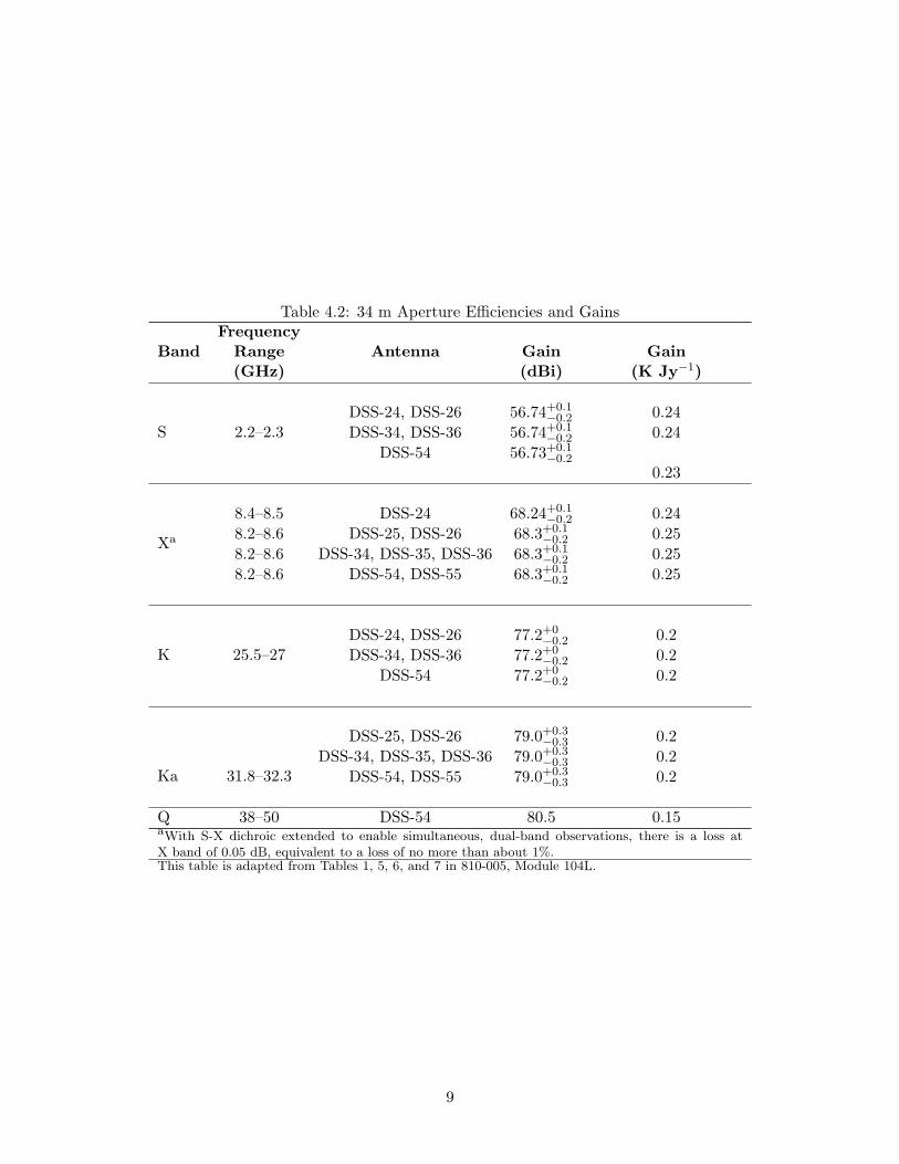
Table 4.2: 34 m Aperture Efficiencies and GainsFrequency

Band Range Antenna Gain Gain(GHz) (dBi) (K Jy−1)

S 2.2–2.3DSS-24, DSS-26 56.74+0.1

−0.2 0.24

DSS-34, DSS-36 56.74+0.1−0.2 0.24

DSS-54 56.73+0.1−0.2

0.23

Xa

8.4–8.5 DSS-24 68.24+0.1−0.2 0.24

8.2–8.6 DSS-25, DSS-26 68.3+0.1−0.2 0.25

8.2–8.6 DSS-34, DSS-35, DSS-36 68.3+0.1−0.2 0.25

8.2–8.6 DSS-54, DSS-55 68.3+0.1−0.2 0.25

K 25.5–27DSS-24, DSS-26 77.2+0

−0.2 0.2

DSS-34, DSS-36 77.2+0−0.2 0.2

DSS-54 77.2+0−0.2 0.2

Ka 31.8–32.3

DSS-25, DSS-26 79.0+0.3−0.3 0.2

DSS-34, DSS-35, DSS-36 79.0+0.3−0.3 0.2

DSS-54, DSS-55 79.0+0.3−0.3 0.2

Q 38–50 DSS-54 80.5 0.15aWith S-X dichroic extended to enable simultaneous, dual-band observations, there is a loss atX band of 0.05 dB, equivalent to a loss of no more than about 1%.This table is adapted from Tables 1, 5, 6, and 7 in 810-005, Module 104L.

9

Table 4.3: 34 m Antenna Beam WidthsBeam

Band Antenna Width

S DSS-24, DSS-26, DSS-34, DSS-36, DSS-54 14.5′

X all 4′

K DSS-24, DSS-34, DSS-36, DSS-54 1.3′

Ka DSS-25, DSS-26, DSS-34, DSS-35, DSS-36, DSS-54, DSS-55 1′

Q DSS-54 43′′

This table is adapted from Tables 5, 6, and 7 in 810-005, Module 104L.

Further, at K-, Ka-, and Q bands, the antenna gains can be affected significantly by the zenithopacity due to the amount of water vapor in the atmosphere above the antenna. Under generallyclear conditions, the additional zenith opacity does not exceed 5% at either band. However, undercloudy conditions zenith opacities can be 10%. In general, opacities tend to be lowest at Goldstone,due to its arid climate, and highest at Canberra, with Madrid showing intermediate values.

4.3 Resolution

Table 4.3 summarizes the half-power beamwidth of the antennas for the specific operational fre-quencies.

4.4 Polarization

In general, only a single polarization is available, which can be either right circular polarization(RCP) or left (LCP). Table 4.4 summarizes the antennas for which there are exceptions.

10

Table 4.4: 34 m Antenna Polarization CapabilitiesAntenna Band Polarization

DSS-24 (Goldstone) X RCP and LCPDSS-25 (Goldstone) X RCP and LCPa

DSS-26 (Goldstone) X RCP and LCPDSS-34 (Canberra) X RCP and LCPDSS-35 (Canberra) X RCP and LCPDSS-35 (Canberra) X RCP and LCPDSS-55 (Madrid) X RCP and LCP

DSS-25 (Goldstone) Ka RCP and LCPDSS-26 (Goldstone) Ka RCP and LCPDSS-34 (Canberra) Ka RCP and LCPDSS-35 (Canberra) Ka RCP and LCPDSS-36 (Canberra) Ka RCP and LCPDSS-54 (Madrid) Ka RCP and LCPDSS-55 (Madrid) Ka RCP and LCP

DSS-54 (Madrid) Q RCP and LCP

If not listed, an antenna should be assumed to have only either RCP or LCP.aOne, selectable polarization will have less sensitivity than the other

This table is adapted from Table 1 in 810-005, Module 104L.

11

Chapter 5

Receiving Systems

Echoing the discussion in §3.2, the current suite of receivers reflects both the DSN’s mission forspacecraft tracking and historical precedent. The order of this section is in terms of those receiversand bands developed primarily for radio astronomy observations followed by those that are standardfor spacecraft TT&C but also available for radio astronomical observations.

5.1 Radio Astronomical K Band (17 GHz–27 GHz)

DSS-43 is equipped with a radio astronomical system operating in the 17 GHz–27 GHz band.Figure 5.1 provides an overview of the system, and Figures 5.2–5.3 show the major components ofthe system. Kuiper et al. (2019) provide a more detailed description of this system.

The LNA Assembly (or “front-end”) contains two feed horns, allowing for simultaneous ob-servations of both a target source and a secondary position (e.g., for calibration purposes). Eachfeed horn produces linear polarization, and the two feed horns are separated by 2.1′ (equivalentto 2.8 half-power beamwidths at 22 GHz). Each linear polarization from each feed horn is con-nected to a cryogenic LNA. Ambient temperature microwave absorbers and phase calibrationsignals (with 1 MHz or 4 MHz frequency combs) can be inserted into the signal path for calibrationpurposes.

The Downconverter receives the output from the LNA Assembly and produces intermediatefrequencies (IFs). There are four signal chains (labelled E1, H1, E2, and H2 for the E- and H-plane polarizations of Feeds 1 and 2), and switches allow the signals to be switched in a manner tocancel gain profiles. Each signal chain is then passed to a set of bandpass filters, producing 2 GHzsub-bands centered at 18 GHz, 20 GHz, 22 GHz, 24 GHz, and 26 GHz. Following the bandpassfilters, polarization converters allow the signals to be converted from linear polarization to circularpolarization, if desired. Finally, local oscillators (LOs) are mixed with the sub-bands to produce1 GHz IFs. These 1 GHz IFs are then transported by fiber optic cables from the antenna to theSignal Processing Center for detection and post-processing.

Estimates of the receiver temperature, extrapolated to outside the atmosphere, are TRX = 29 K,with approximately 10% uncertainty or variation from feed-polarization channel to channel. Undernear-ideal conditions (clear skies and cold ambient temperatures), total system temperatures Tsys

approaching 40 K have been measured.

12

5.2 Radio Astronomical Q Band (38 GHz–50 GHz)

The DSS-54 (34 m) antenna at the Madrid DSCC is equipped with a Q band receiving system, de-veloped under the auspices of the Spanish host country radio astronomy community. This materialis extracted from a larger discussion by Rizzo et al. (2012).

The Q-band front-end has a useful frequency range of 38 GHz–50 GHz per polarization. At thefront-end, the band is mixed with an LO at 62 GHz, providing 12 GHz of transported bandwidthfrom 12 GHz to 24 GHz. At the IF processor, this transported bandwidth is split into two 8 GHzwide sub-bands (labeled LO and HI, respectively). The LO sub-band is 12 GHz–20 GHz, and theHI sub-band is 18 GHz–26 GHz. The IF processor further downconverts each sub-band to a tunable1.5 GHz baseband per polarization.

The final output of the Q-band system is thus four simultaneous signals, 1.5 GHz baseband right-and left-circular polarization in the HI sub-band (mapping to sky frequencies 44 GHz–38 GHz)and 1.5 GHz baseband right- and left-circular polarization in the LO sub-band (mapping to skyfrequencies 42 GHz–50 GHz). Because of the processing within the IF processor, the HI sub-bandsignals are mirrored in frequency.

5.3 L Band (1628 MHz–1708 MHz)

The 70 m antennas are equipped with an L-band feed, normally configured to receive left circularpolarization (LCP) though, with sufficient advance notice, it can be reconfigured (manually) toreceive RCP. The position of the L-band feed requires that the antenna subreflector be rotated toilluminate the L-band feed, which prevents other frequencies from being simultaneously available.

For DSS-14 and DSS-63, the L-band feed is a so-called “Potter horn” (Potter 1963), whichis a relatively narrowband design optimized for 1.668 GHz and a single polarization. Experiencesuggests that somewhat wider bandwidths than the original design may be able to be obtained.

For DSS-43, a “wide-band” feed was designed (Hoppe et al. 2015) and installed. However,current plans are that this feed will be removed as part of the 2020 Depot Level Maintenance ofDSS-43; whether it will be reinstalled is not yet determined.

The low-noise amplifiers (LNAs) are cooled HEMT devices, with typical noise temperaturesof 27 K.

After amplification, the L-band signal is up-converted to S band and sent to the S-band Sig-nal Distribution Assembly for subsequent downconversion and transmission through the S-bandtransmission system.

5.4 S Band (2200 MHz–2300 MHz)

All 70 m antennas and at least one 34 m antenna at each Complex are equipped with S-bandreceiving systems. These systems are designed primarily for spacecraft TT&C, hence their relativelynarrow bandwidths relative to current radio astronomical systems.

The main reflector illuminates the S-band feed via an S-X dichroic plate. Following the feed is anorthomode junction, enabling dual polarization observations. However, because of the TT&C needs,one of the polarizations is always fed to a diplexer resulting in a slightly higher system temperaturefor that polarization (≈ 10% higher). The signals are then amplified by an LNA, cooled HEMTdevices, and fed to the S-band signal distribution assembly before being downconverted to anintermediate frequency (IF) for signal transport (Chap. 6).

13

Typical (zenith) system temperatures are 17 K (DSS-14 and DSS-43) and 20 K (DSS-63).Because of the S-X dichroic plate, there is also a configuration enabling dual frequency-singlepolarization observations between S- and X bands. The dual S-X capability increases the noiseS-band temperature by approximately 5 K.

Experience suggests that the S-band systems can be affected significantly by radio frequencyinterference (RFI).

5.5 X Band (8200 MHz–8600 MHz)

All 70 m antennas and at least one 34 m antenna at each Complex are equipped with X-bandreceiving systems. These systems are designed primarily for spacecraft TT&C, hence their relativelynarrow bandwidths relative to current radio astronomical systems. In particular, the X-bandcoverage at DSS-24 is even more restricted than the general 34 m antennas, being restricted to therange 8400 MHz–8500 MHz.

The X-band feed is followed by a diplexing junction in order to allow for injection of trans-missions (for spacecraft TT&C), by an orthomode junction in order to enable dual polarizationobservations, and by LNAs that are cooled HEMT devices.

Typical (zenith) system temperatures are 17 K (70 m antennas). With the S-X dichroic plateextended, dual frequency-single polarization observations between S- and X bands. The dual S-X capability increases the X-band noise temperature by approximately 1 K.

5.6 Spacecraft Tracking K Band (25.5 GHz–27 GHz)

Within the DSN, this band is also called the “near-Earth Ka band” or the “Ka2 band.”At least one 34 m antenna at each Complex is equipped with a K-band receiving system. These

systems are designed primarily for spacecraft TT&C, hence their relatively narrow bandwidthsrelative to current radio astronomical systems.

This receiving system can be used in combination with the TT&C S-band receiving system(§5.4).

5.7 Ka Band (31.8 GHz–32.3 GHz)

Most of the 34 m antenna at each Complex are equipped with a Ka-band receiving system. Thesesystems are designed primarily for spacecraft TT&C, hence their relatively narrow bandwidthsrelative to current radio astronomical systems.

This receiving system can be used in combination with the TT&C X-band receiving system(§5.4. The simultaneous reception of X- and Ka-band signals involves the extension of a dichroicplate, which produces a small decrease in the antenna gain (approximately 0.15 dBi).

14

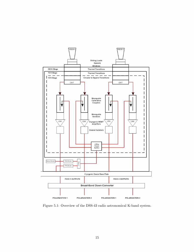
Figure 5.1: Overview of the DSS-43 radio astronomical K-band system.

15

Figure 5.2: Low-noise assembly (“front-end”) for the DSS-43 K-band system. Visible are the twofeeds at top, the waveguide calibration couplers (vertical rectangular units), and the plane on whichthe LNAs and 4-way power splitter are mounted.

16

Figure 5.3: Downconverter for the DSS-43 K-band system.(left) Block diagram;(right) Rotated viewof the unit prior to mounting on the antenna. Matching the orientation of the above schematic, thefour inputs from the outputs of the feed horns are on the top of this image, with signals traveling“downward.” The downconverter modules, producing the 40 IF outputs, are the green boxes atthe bottom.

17

Chapter 6

Signal Transport

Following conditioning at the antenna, the signals are downconverted from the sky frequency toan intermediate frequency (IF). The (analog) IF signals are transported over fiber optic linksfrom the antenna to the Signal Processing Center (SPC). Typically, the IF is 500 MHz wide,from 100 MHz to 600 MHz, though it can be narrower at S band. (The S-band allocation for deepspace telecommunications is only 10 MHz wide.)

Radio astronomical systems can employ slightly different signal transport systems than thestandard DSN systems, but the overall signal flow is substantially similar.

Figures 6.1–6.2 provide a graphical view of the signal transport from the antennas to the variousprocessing backends for each Complex. For clarity, two figures are shown for each complex, one forthe 70 m antenna at that Complex and one for the 34 m beam waveguide antennas.

For the DSS-43 K-band system, following downconversion, the signals are transported in 1 GHzbands over fiber optic links to the Canberra Signal Processing Center.

18

Figure 6.1: top Signal transport for DSS-43 at the CDSCC.bottom Signal transport for 34 m beamwaveguide antennas at the CDSCC. Not every 34 m beam waveguide antenna offers all frequencies,viz. Table 4.2.

19

Figure 6.2: top Signal transport for DSS-63 at the MDSCC.bottom Signal transport for 34 m beamwaveguide antennas at the MDSCC. Not every 34 m beam waveguide antenna offers all frequencies,viz. Table 4.2.

20

Chapter 7

Backends

The various DSN Complexes host different processing backends, dictated largely by previous sci-entific interests of Caltech and JPL staff and external users. Each backend is summarized briefly;in many cases, there are more detailed publications providing additional information.

For the backends at Canberra, they are typically configured to work with the radio astronomicalK-band system, though, in principle, they can accept input from any of the available bands (radioastronomical or spacecraft TT&C) at the Complex (Chapter 5).

The development of additional backends or user-provided backends is both feasible and en-couraged. Interested individuals should contact DSN Radio Astronomy staff for discussions andassessment of feasibility.

7.1 Fast Fourier Transform Spectrometer (FFTS)-Madrid

The Fast Fourier Transform Spectrometer (FFTS) is a Spanish host-country backend, installed atthe Madrid Complex. This material is extracted from a longer description by Rizzo et al. (2012).

The FFTS accepts four analog 1.5 GHz baseband inputs, corresponding to the right- and left-circularly polarized HI and LO sub-bands for the Madrid Complex (§5.2). Each baseband is digi-tized, with an 8-bit digitizer, and then transformed to the frequency domain via a four-tap polyphasefilterbank. The default configuration is 8192 frequency channels, providing 183 kHz spectral reso-lution across the full 1.5 GHz bandwidth, equivalent to a velocity resolution of 1.24 km s−1 at afiducial frequency of 44 GHz. Higher spectral resolutions across a narrower bandwidth may also beavailable upon request.

7.2 DSN Pulsar Processor-Canberra

The DSN Pulsar Processor is installed at the Canberra Complex. This material is extracted froma longer description by Kocz et al. (2016).

The pulsar processor provides both timing (coherent) and searching (incoherent) modes. Insearching mode, a 1024-pt filterbank is obtained. Sampling times are frequency dependent, butcan range from 32 µs to 512 µs. For timing mode, real-time dedispersion is conducted. However,experience shows that RFI can affect the usable bandwidth, which can in turn affect sampling timesand dispersion measures that can be observed.

21

Table 7.1: DSN Radio Astronomy Spectrometer modesMode Summary

1 32k spectral points, FFT-based2 8k spectral points, polyphase filter-based3 512k spectral points [TBC]

7.3 DSN Radio Astronomy Spectrometer-Canberra

The DSN Radio Astronomy Spectrometer is installed at the Canberra Complex. It is designedspecifically to accommodate the output of the Radio Astronomical K-band system, but, in principle,can process any of the outputs from any of the systems at the Canberra Complex. Table 7.1summarizes the available modes for this spectrometer.

Data from the Radio Astronomy Spectrometer will be provided in single-dish FITS (SDFITS)format (Garwood 2000) in a series of levels reflecting increasing data processing.

7.3.1 Level 0 Data

The header contains relevant data about the antenna and details of the observations.The primary data consist of the spectra acquired during the observation, with each entry being

the spectrum for each scan.Additional data tables (structured as FITS BINTABLE) are provided, which contain information

about the observation that is used for subsequent processing to higher level data products. Onedata table provides the antenna’s elevation as a function of time during each scan, and a seconddata table provides an estimate of the system temperature Tsys as a function of time during eachscan.

7.3.2 Level 1 Data

These data products are intended to be a notional processing of the Level 0 data, in a mannerthat is consistent with producing data products sufficient for analysis and publication but alsofor alternate or additional processing. The intent is to provide a basic estimate of the antennatemperature using the standard position-switching technique,

T ∗ant =

Ton − Toff

ToffTsys, (7.1)

where Ton is the measured temperature (power) toward a source, Toff is the measured temperature(power) toward an “off” position, and Tsys is the system temperature.

Level 1a Data

The Level 1a data product performs the first portion of the calibration, forming the factor Ton − Toff/Toff

using the nearest-neighbor “off” scan. This division in the calibration is structured in this mannerfor a number of motivations. With this initial “ON−OFF” calculation an investigator can assessthe calibration at this stage, there may be some cases in which only relative calibration (withoutthe system temperature) may be valuable, and there are alternate approaches to identifying the“off” scan (e.g., linear interpolation between the two “off” scans nearest in time).

22

Level 1b Data

The Level 1b data product uses the Level 1a data product and an estimate of the system temper-ature Tsys to form the antenna temperature T ∗

ant of equation (7.1).

7.4 VLBI Radio Astronomy (VRA) Assembly

This backend is planned for deployment into the DSN in 2021. It will provide high-bandwidthrecording, with data rates up to 2 Gbps.

For radio astronomical purposes, data can be obtained in the VLBI Data Interchange Format(VDIF).

23

Appendix A

Proposal Preparation andObservation Planning

This appendix is designed to provide a variety of information that proposers may find useful indeveloping a proposal or planning observations.

Figures A.1, A.2, and A.3 show the visibilities of sources as a function of hour angle and decli-nation. These guides should be taken as approximate. All of the Complexes have local topographythat can restrict the lowest available elevation at some azimuths. DSN Telecommunications In-terfaces Module 301L (2019) provides specific elevation limits, as a function of hour angle, forindividual antennas as well as precise antenna locations in various coordinate systems.

24

Figure A.1: Visibility of sources from the Canberra Deep Space Communications Complex. Theabscissa is the hour angle, and the ordinate is the elevation. The different curves are labeled bythe declination of a source.

25

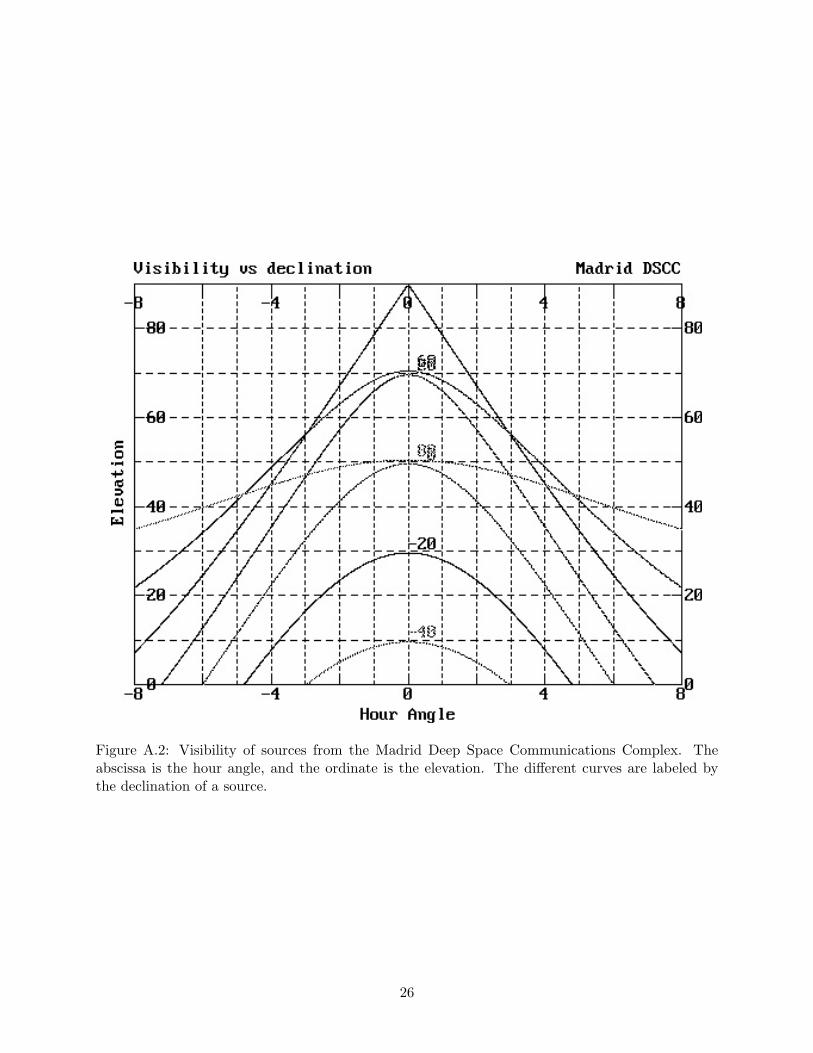
Figure A.2: Visibility of sources from the Madrid Deep Space Communications Complex. Theabscissa is the hour angle, and the ordinate is the elevation. The different curves are labeled bythe declination of a source.

26

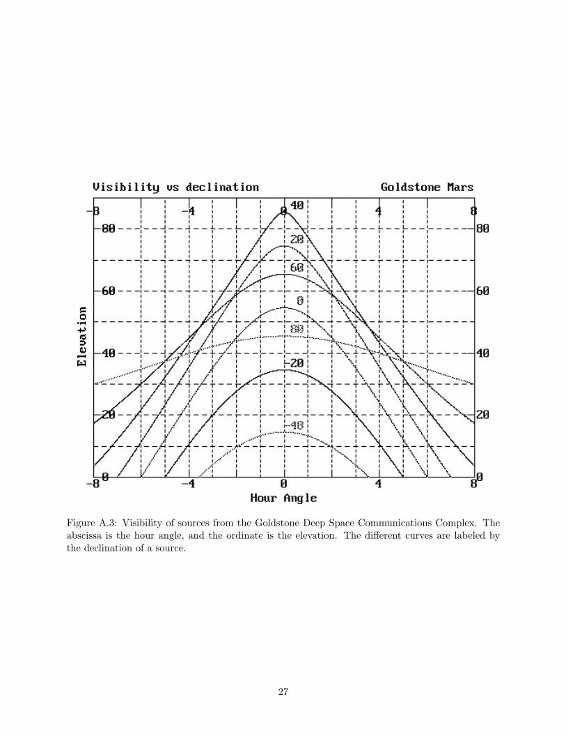
Figure A.3: Visibility of sources from the Goldstone Deep Space Communications Complex. Theabscissa is the hour angle, and the ordinate is the elevation. The different curves are labeled bythe declination of a source.

27

Bibliography

Charlot, P., et al. 2020, Astron. & Astrophys., in preparation; http://hpiers.obspm.fr/icrs-pc/newwww/icrf/icrf3-ReadMe.txt

Cohen, M. H., Cannon, W., Purcell, G. H., Shaffer, D. B., Broderick, J. J., Kellermann, K. I., &Jauncey, D. L. 1971, “The Small-Scale Structure of Radio Galaxies and Quasi-Stellar Sourcesat 3.8 Centimeters,” Astrophys. J., 170, 207; doi: 10.1086/151204

Deep Space Network Telecommunications Interfaces, DSN No. 810-005;http://deepspace.jpl.nasa.gov/dsndocs/810-005/

Dvorsky, J., Renzetti, N., & Fulton, D. 1992, “The Goldstone Solar System Radar: A ScienceInstrument for Planetary Research,” JPL Publication 92-29 (Jet Propulsion Laboratory, Cali-fornia Institute of Technology: Pasadena, CA)

Fey, A. L., Gordon, D., Jacobs, C. S., et al. 2015, “The Second Realization of the InternationalCelestial Reference Frame by Very Long Baseline Interferometry,” Astron. J., 150, 58; doi:10.1088/0004-6256/150/2/58

Hoppe, D. J., Khayatian, B., Lopez, B., Torrez, T., Long, E., Sosnowski, J., Franco, M., & Teit-elbaum, L. 2015, “Broadband Upgrade for the 1.668-GHz (L-Band) Radio Astronomy FeedSystem on the DSN 70-m Antennas,” IPN Progress Report 42-202, Jet Propulsion Laboratory,Pasadena, CA

Garwood, R. W. 2000, “SDFITS: A Standard for Storage and Interchange of Single Dish Data,”in Astronomical Data Analysis Software and Systems IX, Astronomical Society of the PacificConference Proceedings, Vol. 216, eds. N. Manset, C. Veillet, & D. Crabtree (AstronomicalSociety of the Pacific: San Francisco) p. 243; ISBN 1-58381-047-1

Guzman-Ramirez, L., Rizzo, J. R., Zijlstra, A. A., Garcıa-Miro, C., Morisset, C., & Gray, M. D.2016, “First detection of 3He+ in the planetary nebula IC 418,” Mon. Not. R. Astron. Soc.,460, L35; doi: 10.1093/mnrasl/slw070

Imbriale, W. A. 2003, Large Antennas of the Deep Space Network, Volume 4, Deep Space Commu-nications and Navigation Series, ed. J. H. Yuen, Jet Propulsion Laboratory, California Instituteof Technology; (John Wiley & Sons: San Francisco, CA) ISBN: 978-0-471-44537-1

Kocz, J., Majid, W., White, L., Snedeker, L., & Franco, M. 2016, “Pulsar Timing at the Deep SpaceNetwork,” J. Astron. Inst., 05, 1641013; doi: https://doi.org/10.1142/S2251171716410130

Kuiper, T. B. H., Langer, W. D., & Velusamy, T. 1996, “Evolutionary Status of the Pre-protostellarCore L1498,” Astrophys. J., 468, 761; doi: 10.1086/177732

28

uiper, T. B. H., Franco, M., Smith, S., Baines, G., Greenhill, L. J., Horiuchi, S., Olin, T., Price,D. C., Shaff, D., Teitelbaum, L. P., Weinreb, S., White, L., & Zaw, I. 2019, “The 17–27 GHzDual Horn Receiver on the NASA 70 m Canberra Antenna,” J. Astron. Inst., 8, 1950014; doi:10.1142/S2251171719500144

Levy, G. S., Linfield, R. P., Ulvestad, J. S., et al. 1986, “Very long baseline interferometricobservations made with an orbiting radio telescope,” Science, 234, 187; doi: 10.1126/sci-ence.234.4773.187

Levy, G. S., Linfield, R. P., Edwards, C. D., et al. 1989, “VLBI using a telescope in Earth orbit. I- The observations,” Astrophys. J., 336, 1098; doi: 10.1086/167080

Linfield, R. P., Levy, G. S., Ulvestad, J. S., et al. 1989, “VLBI using a telescope in Earth orbit. II -Brightness temperatures exceeding the inverse Compton limit,” Astrophys. J., 336, 1105; doi:10.1086/167081

Potter, P. D. 1963, “A New Horn Antenna with Suppressed Sidelobes and Equal Beamwidths,”JPL Technical Report 32-354, Jet Propulsion Laboratory, Pasadena, CA

Rizzo, J. R., Pedreira, A., Garcıa Mio, Sotuela, .I, Kuiper, T. B. H., Cernicharo, J., Castro Cero,J. M, Larranag,a J. R., &Ojalvo, L. 2012, “The wideband backend for host country radio astron-omy in the Spanish DSN Robledo complex,” in Proc. SPIE 8452, Millimeter, Submillimeter, andFar-Infrared Detectors and Instrumentation for Astronomy VI, 84522S; doi: 10.1117/12.926085

Slade, M. A., Benner, L. A., & Silva, A. 2011, “Goldstone Solar System Radar Observatory: Earth-Based Planetary Mission Support and Unique Science Results,” Proc. IEEE, 99

Velusamy, T., Kuiper, T. B. H., & Langer, W. D. 1995, “CCS Observations of the ProtostellarEnvelope of B335,” Astrophysical Journal, 451, L75; doi: 10.1086/309691

29