Embed Size (px)
Citation preview

Journal of Development Economics 29 (1988) 271-306. North-Holland
THE DEBT CRISIS*
Structural Explanations of Country Performance
Andrew BERG
Massachusetts Institute of Technology, Cambridge, MA 02139, USA
Jeffrey SACHS
Harvard University, Cambridge, MA 02138, VSA
This paper develops a cross-country statistical model of debt rescheduling, and the secondary market valuation of LDC debt, which links these variables to key structural characteristics of developing countries, such as the trade regime, the degree of income inequality, and the share of agriculture in GNP. Our most striking finding is that higher income inequality is a significant predictor of a higher probability of debt rescheduling in a cross-section of middle-income countries. We attribute this correlation to various difliculties of political management in economies with extreme inequality. We also find that outward-orientation of the trade regime is a significant predictor of a reduced probability of debt rescheduling.
1. Introduction
The debt crisis can be studied as a problem in epidemiology. A powerful virus, high world interest rates, hit the population of capital-importing developing countries in the early 1980s. Some countries succumbed to the virus, having to reschedule their debts on an emergency basis, while others did not. And of those countries that arrived for emergency treatment, some recovered sufftciently to enter a period of quiet convalescence, while others are still suffering from febrile seizures in the IMF’s intensive care unit.
The epidemiologist studies the progression of a disease in order to understand the disease better, and to recommend improved forms of treatment. For the same reason, it is important to understand why some countries fell prey to the debt crisis while others did not, and why some countries have recovered from the crisis while other countries remain deeply enmeshed in it. The goal of our paper is to find answers to these questions, and then to draw inferences about the fundamental nature of the debt crisis itself. Was the crisis mainly the result of external shocks, internal policy mistakes, the organization of political power within the debtor countries, or
*We are grateful to the participants in the First InterAmerican Seminar on Economics, and in particular to Albert Fishlow and our discussants Marcel0 Selowsky and Ernest0 Zedillo. Andrew Berg acknowledges linancial support from an NSF Graduate Fellowship. The research supported here is part of the NBER’s research program in International Studies. Any opinions expressed are those of the authors and not those of the National Burea of Economic Research.
030~3878/88/$3.50 0 1988, Elsevier Science Publishers B.V. (North-Holland)
212 A. Berg and J. Sachs, The debt crisis
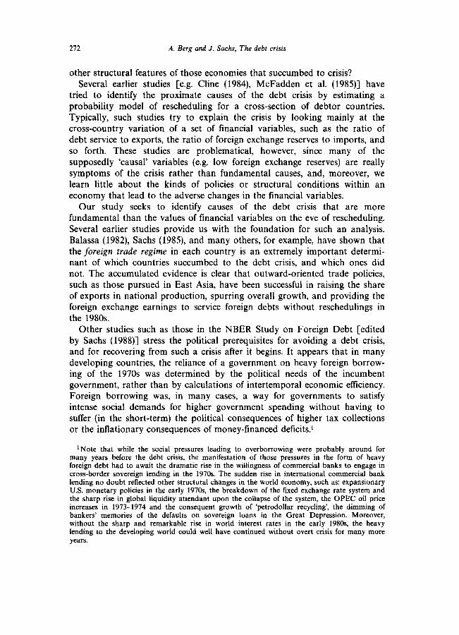
other structural features of those economies that succumbed to crisis? Several earlier studies [e.g. Cline (1984), McFadden et al. (1985)] have
tried to identify the proximate causes of the debt crisis by estimating a probability model of rescheduling for a cross-section of debtor countries. Typically, such studies try to explain the crisis by looking mainly at the cross-country variation of a set of financial variables, such as the ratio of debt service to exports, the ratio of foreign exchange reserves to imports, and so forth. These studies are problematical, however, since many of the supposedly ‘causal’ variables (e.g. low foreign exchange reserves) are really symptoms of the crisis rather than fundamental causes, and, moreover, we learn little about the kinds of policies or structural conditions within an economy that lead to the adverse changes in the financial variables.
Our study seeks to identify causes of the debt crisis that are more fundamental than the values of financial variables on the eve of rescheduling. Several earlier studies provide us with the foundation for such an analysis. Balassa (1982), Sachs (1985), and many others, for example, have shown that the foreign trade regime in each country is an extremely important determi- nant of which countries succumbed to the debt crisis, and which ones did not. The accumulated evidence is clear that outward-oriented trade policies, such as those pursued in East Asia, have been successful in raising the share of exports in national production, spurring overall growth, and providing the foreign exchange earnings to service foreign debts without reschedulings in the 1980s.
Other studies such as those in the NBER Study on Foreign Debt [edited by Sachs (1988)] stress the political prerequisites for avoiding a debt crisis, and for recovering from such a crisis after it begins. It appears that in many developing countries, the reliance of a government on heavy foreign borrow- ing of the 1970s was determined by the political needs of the incumbent government, rather than by calculations of intertemporal economic efficiency. Foreign borrowing was, in many cases, a way for governments to satisfy intense social demands for higher government spending without having to suffer (in the short-term) the political consequences of higher tax collections or the inflationary consequences of money-financed deficits.’
‘Note that while the social pressures leading to overborrowing were probably around for many years before the debt crisis, the manifestation of those pressures in the form of heavy foreign debt had to await the dramatic rise in the willingness of commercial banks to engage in cross-border sovereign lending in the 1970s. The sudden rise in international commercial bank lending no doubt reflected other structural changes in the world economy, such as: expansionary U.S. monetary policies in the early 1970s the breakdown of the fixed exchange rate system and the sharp rise in global liquidity attendant upon the collapse of the system, the OPEC oil price increases in 1973-1974 and the consequent growth of ‘petrodollar recycling’, the dimming of bankers’ memories of the defaults on sovereign loans in the Great Depression. Moreover, without the sharp and remarkable rise in world interest rates in the early 198Os, the heavy lending to the developing world could well have continued without overt crisis for many more years.
A. Berg and J. Sachs, The debt crisis 273
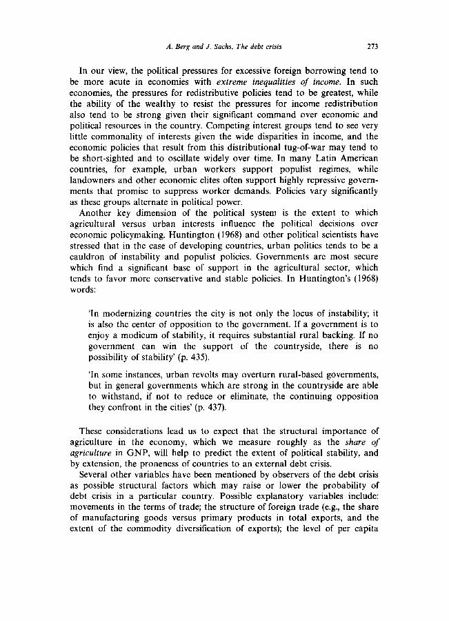
In our view, the political pressures for excessive foreign borrowing tend to be more acute in economies with extreme inequalities of income. In such economies, the pressures for redistributive policies tend to be greatest, while the ability of the wealthy to resist the pressures for income redistribution also tend to be strong given their significant command over economic and political resources in the country. Competing interest groups tend to see very little commonality of interests given the wide disparities in income, and the economic policies that result from this distributional tug-of-war may tend to be short-sighted and to oscillate widely over time. In many Latin American countries, for example, urban workers support populist regimes, while landowners and other economic elites often support highly repressive govern- ments that promise to suppress worker demands. Policies vary significantly as these groups alternate in political power.
Another key dimension of the political system is the extent to which agricultural versus urban interests influence the political decisions over economic policymaking. Huntington (1968) and other political scientists have stressed that in the case of developing countries, urban politics tends to be a cauldron of instability and populist policies. Governments are most secure which find a significant base of support in the agricultural sector, which tends to favor more conservative and stable policies. In Huntington’s (1968) words:
‘In modernizing countries the city is not only the locus of instability; it is also the center of opposition to the government. If a government is to enjoy a modicum of stability, it requires substantial rural backing. If no government can win the support of the countryside, there is no possibility of stability’ (p. 435).
‘In some instances, urban revolts may overturn rural-based governments, but in general governments which are strong in the countryside are able to withstand, if not to reduce or eliminate, the continuing opposition they confront in the cities’ (p. 437).
These considerations lead us to expect that the structural importance of agriculture in the economy, which we measure roughly as the share of agriculture in GNP, will help to predict the extent of political stability, and by extension, the proneness of countries to an external debt crisis.
Several other variables have been mentioned by observers of the debt crisis as possible structural factors which may raise or lower the probability of debt crisis in a particular country. Possible explanatory variables include: movements in the terms of trade; the structure of foreign trade (e.g., the share of manufacturing goods versus primary products in total exports, and the extent of the commodity diversification of exports); the level of per capita
214 A. Berg and J. Sachs, The debt crisis
income in the country; and the geographical location of the country, especially if there are regional ‘contagion effects’ in commercial bank lending.
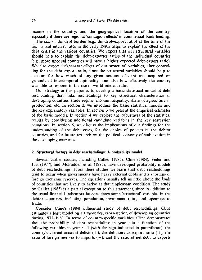
The size of the debt burden (e.g., the debt-export ratio) at the time of the rise in real interest rates in the early 1980s helps to explain the effect of the debt crisis in the various countries. We expect that our structural variables should help to explain the debtexporter ratios of the individual countries (e.g., more unequal countries will have a higher expected debt&export ratio). We also expect independent effects of our structural variables, after control- ling for the debt-export ratio, since the structural variables should help to account for how much of any given amount of debt was acquired on grounds of intertemporal optimality, and also how effectively the country was able to respond to the rise in world interest rates.
Our strategy in this paper is to develop a basic statistical model of debt rescheduling that links reschedulings to key structural characteristics of developing countries: trade regime, income inequality, share of agriculture in production, etc. In section 2, we introduce the basic statistical models and the key explanatory variables. In section 3 we present the empirical estimates of the basic models. In section 4 we explore the robustness of the statistical results by considering additional candidate variables in the key regression equations. In section 5, we discuss the implications of our findings for the understanding of the debt crisis, for the choice of policies in the debtor countries, and for future research on the political economy of stabilization in the developing countries.
2. Structural factors in debt reschedulings: A probability model
Several earlier studies, including Callier (1985), Cline (1984), Feder and Just (1977), and McFadden et al. (1985), have developed probability models of debt reschedulings. From these studies we learn that debt reschedulings tend to occur when governments have heavy external debts and a shortage of foreign exchange reserves. The equations usually tell us little about the kinds of countries that are likely to arrive at that unpleasant condition. The study by Callier (1985) is a partial exception to this statement, since in addition to the usual financial indicators he consideres some ‘structural’ variables in the debtor countries, including population, investment rates, and openness to trade.
Consider Cline’s (1984) influential study of debt reschedulings. Cline estimates a logit model on a time-series, cross-section of developing countries during 1972-1983. In terms of country-specific variables, Cline demonstrates that the probability of debt rescheduling in year t is a function of the following variables in year t- 1 (with the sign indicated in parentheses): the country’s current account deficit (+), the debt serviceexport ratio (+), the ratio of foreign reserves to imports (-), and the ratio of net debt to exports

A. Berg and J. Sachs, The debt crisis 275
(+). Other structural variables that Cline includes in his model, such as the economy’s growth rate, per capita income level, and savings rate, turn out to have little explanatory power.
Our approach differs from Cline’s treatment by attempting, like Callier, to relate debt reschedulings to deeper structural characteristics of the econo- mies, characteristics which change slowly over the course of a decade and thus can be considered as temporarily prior to the financial distress itself. In general, where the data are available we measure these structural characteris- tics during the 1970s (e.g., as an average for 197&1980), to emphasize that we are looking at country characteristics that preceded the debt crisis itself.
We develop two basic probability models, the first for the onset of the debt crisis, and the second for the difficulties of the various countries in overcoming the crisis. The first model is a standard cross-section probit model of rescheduling, of the form
Prob (Ri = 1) = @(Zip),
where Ri is a variable equal to 1 if country i rescheduled its debt during 1982-1987, and equal to 0 if there was no rescheduling. The vector Zi includes the economic and political variables in the model. @ is the cumulative standard normal distribution.
The second model is a cobit model, based on the secondary market value of the country’s debt as of July 1987. The idea is as follows. The secondary market value of a country’s debt can be used as a cardinal measure of the country’s creditworthiness. Countries which have escaped the debt crisis will have debt that sells at par or very close to par in the secondary market. Countries enmeshed in the crisis will have debt that sells at a discount relative to par, with the size of the discount providing a good indicator of the political and economic incapacity of the country to service its debt.
A tobit model allows us to test for the factors that determine the size of the discount on the debt, taking into account the fact that for a range of creditworthiness the discount will be zero. The tobit model is specified as follows:
Di=Zi+&i if Di>O,
=o otherwise, (2)
where Di is the discount on the debt and Zi is, as before, the vector of explanatory variables in the model.
Throughout this study, our attention is focussed on commercial borrowers and commercial bank reschedulings, as defined by the World Bank. The World Bank and International Monetary Fund define commercial borrowers as those developing countries for which at least one-third of foreign

276 A. Berg and J. Sachs, The debt crisis
borrowing is from private sector creditors. Thus, we restrict our attention to the subset of developing countries with access to commercial bank lending during the 197Os, and do not analyze the conditions leading to reschedulings of official debt in the Paris Club. While our sample includes a few low- income countries that did have access to commercial loans (e.g., India, Sri Lanka, and China) most of the focus is on middle-income developing countries with per capita incomes above $600 per capita. Even with the restriction to commercial borrowers, the range of countries is enormous, with per capita GNP in 1981 ranging from $260 in India to $5,670 in Trinidad and Tobago.
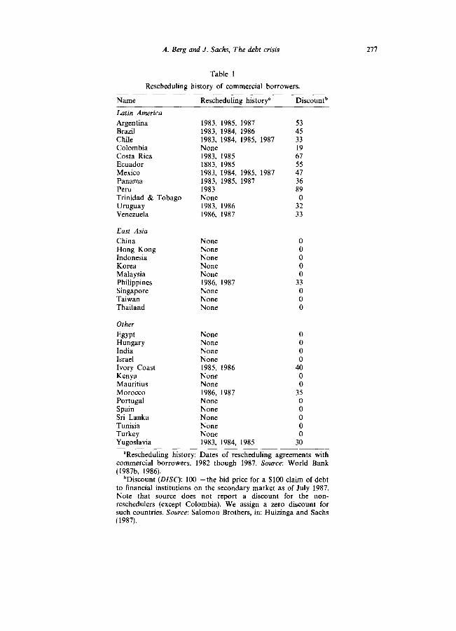
Our sample is further restricted to countries with a population in excess of 1 million in 1980, and to countries for which the key income distributional data are available. The resulting list of countries with their rescheduling histories is shown in table 1. Note that there are 35 countries in the sample, of which 15 have rescheduled with commercial creditors. In Latin America and the Caribbean, ten of twelve countries are reschedulers, with Colombia and Trinidad and Tobago the only two non-reschedulers.* In East Asia, only one of nine countries, the Philippines, is a commercial rescheduler. In sub-Saharan Africa, one of three countries rescheduled (Ivory Coast), while two did not (Kenya and Mauritius). In Europe and North Africa, two out of four countries rescheduled (Morocco and Yugoslavia).
We must stress the severe but inevitable problem of working with a very small sample. Not only are we restricted to a subset of commercial borrowers, but our hypothesis testing is limited by the fact that the number of non-Latin American reschedulers is only five. Note that all of the significance tests reported for the probits and tobits are justified asymptoti- cally. Moreover, it should be recognized that our explanatory variables are no doubt measured with error (especially the distribution of household income, and the index of outward orientation).
We now turn to our principal explanatory variables.
A. Trade regime
There is now a considerable amount of evidence that outward orientation of trade policy enhances the growth prospects of developing countries, as well as their capacity to adjust to external shocks. Several classic studies have addressed the relative merits of outward orientation versus inward, import-substitution policies, as a strategy of long-term development. Vir-
*Colombia has not rescheduled its principal, but it has lost a measure of access to new lending on normal market terms. In 1985, it negotiated a ‘concerted’ loan of $1 billion from the commercial bank creditors, while remaining current on debt servicing obligations. As noted later in the test, we may interpret Colombia as having had a ‘mini-debt crisis’. Interestingly, in our probit model, it turns out that Colombia is almost always estimated to be just on the borderline between rescheduling and non-rescheduling.
A. Berg and J. Sachs, The debt crisis 277
Table 1
Rescheduling history of commercial borrowers.
Name Rescheduling history” Discountb
Latin America
Argentina Brazil Chile Colombia Costa Rica Ecuador Mexico Panama Peru Trinidad & Tobago Uruguay Venezuela
1983, 1985, 1987 53 1983, 1984, 1986 45 1983, 1984, 1985, 1987 33 None 19 1983, 1985 67 1883, 1985 55 1983, 1984, 1985, 1987 47 1983, 1985, 1987 36 1983 89 None 0 1983, 1986 32 1986, 1987 33
East Asia
China Hong Kong Indonesia Korea Malaysia Philippines Singapore Taiwan Thailand
None None None None None 1986, 1987 None None None
Other
Egypt Hungary India Israel Ivory Coast Kenya Mauritius Morocco Portugal Spain Sri Lanka Tunisia Turkey Yugoslavia
None None None None 1985, 1986 None None 1986, 1987 None None None None None 1983, 1984, 1985
0 0 0 0 0
33 0 0 0
0 0 0 0
40 0 0
35 0 0 0 0 0
30
“Rescheduling history: Dates of rescheduling agreements with commercial borrowers, 1982 though 1987. Source: World Bank (1987b, 1986).
“Discount (DISC): 100 -the bid price for a $100 claim of debt to financial institutions on the secondary market as of July 1987. Note that source does not report a discount for the non- reschedulers (except Colombia). We assign a zero discount for such countries. Source: Salomon Brothers, in: Huizinga and Sachs (1987).

278 A. Berg and J. Sachs, The debt crisis
tually all such studies reach the conclusion that outward orientation has produced superior results in the intermediate term [see for example, Little, Scitovsky and Scott (1970), the Bhagwati-Krueger NBER Study (see Krueger (1978) for a summary of the conclusions), and Balassa (1982)]. More recently, several authors have stressed that outward orientation has led not only to better growth performance but also an enhanced ability to adjust to external shocks, including the debt crisis of the 1980s. Balassa (1984) and Sachs (1985) give evidence in support of such a conclusion.
It should be stressed that outward orientation refers to the relative incentives given to the production of exportables versus importables (with a zero bias or a pro-export bias both considered to be outward oriented), and not to the extent to which the trade regime is laissez faire. As argued by many authors, e.g., Bradford (1987), Lin (1985), Sachs (1987), several of the most outward-oriented economies (such as Korea and Taiwan) have highly dirigiste governments, with highly regulated trade. The difference of these countries from the inward-oriented policies elsewhere is that the dirigisme is directed towards export promotion rather than import substitution.
There are several linkages between trade orientation and the probability of debt rescheduling. Most directly, outward-oriented economies have typically maintained a lower ratio of debt service to exports, because of the rapid rise of export earnings. Moreover, outward-oriented economies have tended to maintain exchange rates at levels necessary to maintain export profitability, given that exporters represent a major interest group with strong influence on exchange rate policies. These countries therefore have avoided the political commitments to overvalued exchange rates that characterized many Latin American economies in the late 1970s and early 1980s (e.g., Mexico and Venezuela during 1980-1982), and thus have avoided the worst excesses of capital flight that were produced by exchange rate overvaluations.
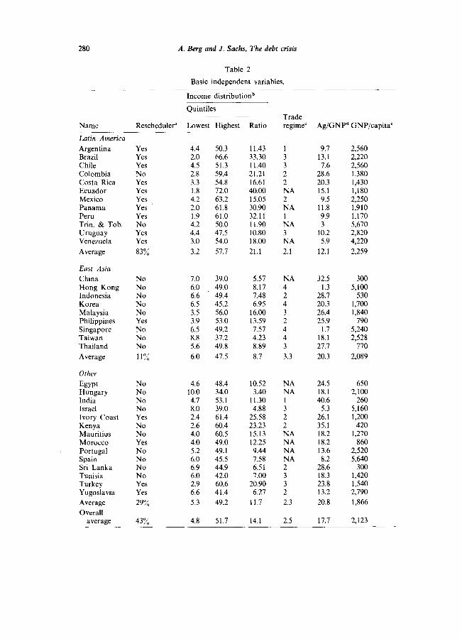
Our basic measure of outward orientation comes from the World Bank (1987) categorization of trade policies in 41 developing countries. The data are reported in the fourth data column of table 2. The World Bank variable divides countries into four categories (strongly outward oriente6moderately outward oriented, moderately inward oriented, and strongly inward oriented), and we use this fourfold division as an index ranging from 1 (most inward oriented) to 4. The great advantage of the World Bank measure over other indicators of the trade regime, such as the growth in exports or the share of exports in GNP, is that it is based on an assessment of trade policies in the developing countries rather than trade outcomes.
It has two major problems however. First, it is available for only 24 of the 35 countries in our sample. To handle this we run two sets of regressions: one with the 24 observations, and one with the 35, but correcting for the missing observations (see details below). The second problem is one of timing. The variable is constructed for the ‘average’ policy orientation during
A. Berg and J. Sachs, The debt crisis 219
196C1973, which is too early for our analysis, and for the average during 1973-1985, which is a bit too late, since it includes years after the onset of the debt crisis. After experimenting with both measures, we have used the later measure despite this timing problem (it turns out that an average over the two periods produces similar results to the variable that we use).
We experimented with other ‘outcome-based’ measures of the trade regime, such as the growth of the export-GNP ratio and the excess of the export- GNP ratio over a predicted value. In general these alternative measures entered the models with the expected sign but often with much less explanatory power than did the World Bank variable. Their use did not change the explanatory power of the other included variables. For the sake of brevity, we do not report the estimates using the alternative measures.
B. Political determinants
For many countries, the debt crisis reflects a political crisis as well as an economic crisis. The political crisis shows up most directly in the inability or unwillingness of governments to restrain large and chronic public sector deficits. In some cases, the large deficits reflect a decline in the legitimacy of a governing party, which attempts to use public spending to maintain political support and to buy off the opposition for as long as possible. In some cases, the regime is so narrowly based and so precarious that it chooses to use the public purse to enrich a small part of the population, aware that political power may slip away at any time. The time horizon of fiscal policymaking becomes short, and the incentives for any particular government in power to balance the budget become extremely weak. In yet other cases, the political process is paralyzed, because power is too widely dispersed among various groups who hold a veto over economic policy, but who cannot coalesce around a consistent economic program.
Because of data limitations, we cannot directly test for the importance of fiscal deficits in the debt crisis, since available cross-country data on budget deficits in developing countries are very poor. Without a detailed analysis of the fiscal data, as in the country monographs in the NBER study on Foreign Debt and Economic Performance; the Country Studies, edited by Sachs (1988b), it is not possible to make a meaningful cross-country comparison of budget deficits.
More generally, it is also not possible to construct clear direct measures of the political determinants of country performance. In particular, we are concerned that political weakness and instability come in many guises. We may observe, for example, continuing political stalemate, a rapid alternation of governments, the attempt of a ruling group to buy off the opposition through unsustainable expansionary macroeconomic policies, political violence, and so forth. We therefore choose to follow a ‘reduced form’ strategy, by identifying two structural characteristics in the economies of the
280 A. Berg and J. Sachs, The debt crisis
Table 2
Basic independent variables.
Income distribution”
Name
Quintiles Trade
Rescheduler” Lowest Highest Ratio regime’ Ag/GNPd GNP/capita’
Latin America
Argentina Brazil Chile Colombia Costa Rica Ecuador Mexico Panama Peru Trin. & Tob. Uruguay Venezuela
Average
East Asia
China Hong Kong Indonesia Korea Malaysia Philippines Singapore Taiwan Thailand
Average
Other
Egypt Hungary India Israel Ivory Coast Kenya Mauritius Morocco Portugal Spain Sri Lanka Tunisia Turkey Yugoslavia
Average
Overall average
Yes Yes Yes No Yes Yes Yes Yes Yes No Yes Yes
83%
4.4 50.3 11.43 1 9.7 2,560 2.0 66.6 33.30 3 13.1 2,220 4.5 51.3 11.40 3 1.6 2,560 2.8 59.4 21.21 2 28.6 1.380 3.3 54.8 16.61 2 20.3 1,430 1.8 72.0 40.00 NA 15.1 1,180 4.2 63.2 15.05 2 9.5 2,250 2.0 61.8 30.90 NA 11.8 1,910 1.9 61.0 32.11 1 9.9 1,170 4.2 50.0 11.90 NA 3 5,670 4.4 47.5 10.80 3 10.2 2,820 3.0 54.0 18.00 NA 5.9 4.220
3.2 51.7 21.1 2.1 12.1 2,259
No 7.0 39.0 5.57 NA 32.5 300 No 6.0 49.0 8.17 4 1.3 5,100 No 6.6 49.4 7.48 2 28.7 530 No 6.5 45.2 6.95 4 20.3 1,700 No 3.5 56.0 16.00 3 26.4 1,840 Yes 3.9 53.0 13.59 2 25.9 790 No 6.5 49.2 1.57 4 1.7 5,240 No 8.8 31.2 4.23 4 18.1 2,528 No 5.6 49.8 8.89 3 27.1 770
11% 6.0 47.5 8.7 3.3 20.3 2,089
No No No No Yes No No Yes No No No No Yes Yes
29%
4.6 48.4 10.52 NA 24.5 650 10.0 34.0 3.40 NA 18.1 2,100 4.7 53.1 11.30 1 40.6 260 8.0 39.0 4.88 3 5.3 5,160 2.4 61.4 25.58 2 26.1 1,200 2.6 60.4 23.23 2 35.1 420 4.0 60.5 15.13 NA 18.2 1,270 4.0 49.0 12.25 NA 18.2 860 5.2 49.1 9.44 NA 13.6 2,520 6.0 45.5 7.58 NA 8.2 5,640 6.9 44.9 6.51 2 28.6 300 6.0 42.0 7.00 3 18.3 1,420 2.9 60.6 20.90 3 23.8 1,540 6.6 41.4 6.27 2 13.2 2,790
5.3 49.2 11.7 2.3 20.8 1,866
43% 4.8 51.7 14.1 2.5 17.7 2,123
A. Berg and J. Sachs, The debt crisis 281
Table 2 continued
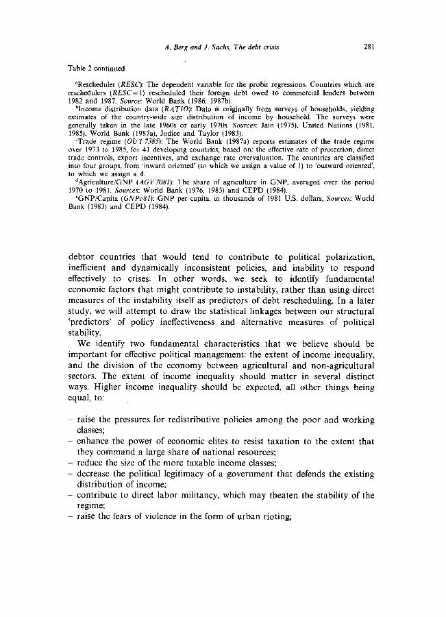
“Rescheduler (RESC): The dependent variable for the probit regressions. Countries which are reschedulers (RESC= 1) rescheduled their foreign debt owed to commercial lenders between 1982 and 1987. Source: World Bank (1986, 1987b).
‘Income distribution data (RATIO): Data is originally from surveys of households, yielding estimates of the country-wide size distribution of income by household. The surveys were generally taken in the late 1960s or early 1970s. Sources: Jain (1975) United Nations (1981, 1985), World Bank (1987a), Jodice and Taylor (1983).
‘Trade regime (OUT7385): The World Bank (1987a) reports estimates of the trade regime over 1973 to 1985, for 41 developing countries, based on: the effective rate of protection, direct trade controls, export incentives, and exchange rate overvaluation. The countries are classified into four groups, from ‘inward oriented (to which we assign a value of 1) to ‘outward oriented’, to which we assign a 4.
“Agriculture/GNP (AGV7081): The share of agriculture in GNP, averaged over the period 1970 to 1981. Sources: World Bank (1976, 1983) and CEPD (1984).
‘GNP/Capita (GNPc81): GNP per capita, in thousands of 1981 U.S. dollars, Sources: World Bank (1983) and CEPD (1984).
debtor countries that would tend to contribute to political polarization, inefficient and dynamically inconsistent policies, and inability to respond effectively to crises. In other words, we seek to identify fundamental economic factors that might contribute to instability, rather than using direct measures of the instability itself as predictors of debt rescheduling. In a later study, we will attempt to draw the statistical linkages between our structural ‘predictors’ of policy ineffectiveness and alternative measures of political stability.
We identify two fundamental characteristics that we believe should be important for effective political management: the extent of income inequality, and the division of the economy between agricultural and non-agricultural sectors. The extent of income inequality should matter in several distinct ways. Higher income inequality should be expected, all other things being equal, to:
_ raise the pressures for redistributive policies among the poor and working classes;
_ enhance the power of economic elites to resist taxation to the extent that they command a large share of national resources;
- reduce the size of the more taxable income classes; - decrease the political legitimacy of a government that defends the existing
distribution of income; - contribute to direct labor militancy, which may theaten the stability of the
regime; _ raise the fears of violence in the form of urban rioting;
282 A. Berg and J. Sachs, The debt crisis
- increase the prospects of a military coup, by requiring a civilian govern- ment to rely on the army to maintain civil peace;
- decrease the support for export-promotion measures that threaten to reduce the labor share of income in the short term;
_ increase the likelihood and importance of capital flight to the extent that financial wealth is highly concentrated;
- more generally, impede the development of a social consensus around policies that promote development in the long term, but which may impose costs on some social groups in the short term.
Thus, one of our central hypotheses is that a high degree of income inequality should be associated with a high probability of rescheduling, since the income inequality undermines the political stability and political effective- ness needed for successful macroeconomic management.
Alesina and Tabellini (1987) have presented a formal model showing how distributional cleavages among competing income classes in a society can contribute to a debt crisis. In their model, a left-wing labor force competes with capitalists for political power (the competition may or may not be via the electoral process). The groups alternate randomly in their hold on power, and both groups recognize that each government’s tenure is likely to be quite short. When labor is in power, it has an interest in squeezing the profits of capitalists, while capitalist governments have the incentive to tax labor heavily.
Whichever group is in power, there is a strong incentive of that govern- ment to borrow up to the lending limit of the foreign banks. This is because the group in power can benefit heavily from an increase in contemporaneous government spending (financed by foreign funds), while there is a good chance that the opposing group will be saddled with the debts, assuming that political power alternates in the future. The shorter is the expected longevity of the government, the greater is the government’s incentive to over-borrow from abroad (relative to the amount that the government would borrow were it certain that it would maintain its hold on government forever). At the same time, the risk of political alternation induces all residents in the economy to hold their wealth outside of the country (i.e., to engage in capital flight), and thereby to keep their wealth beyond the tax collections of the opposing group.
Note that the focus on income distribution as a causal factor in explaining economic performance reverses the usual focus in the development literature on explaining income distribution as the result of government policies and the development process itself. In Adelman and Robinson’s (1987) valuable survey of ‘Income Distribution and Development’, for example, almost the entire focus is on the effects of growth on income distribution, rather than
A. Berg and J. Sachs, The debt crisis 283
the possible effects of income distribution on growth. They focus on the problem that in the growth process in developing countries the income distribution tends to become more unequal before it begins to equalize [as was suggested by Kuznets (1955)], and suggest that there may be an ethical case for equalizing incomes (e.g., via land reform) before the growth process begins (a strategy that Adelman has termed ‘redistribution before growth’, in contrast to ‘redistribution with growth’).
A few authors have adopted the strategy here of reversing the direction of causality, and attempting to explain economic performance as a result of the income distribution. Pyo (1987) Sachs (1987), and Williamson (1987), all suggest that the relatively equal income distribution in East Asia is an important factor in that region’s strong economic performance in the post- War period. For a broad cross-section of developing countries, Pyo shows that the Gini coefficient has a significantly negative effect on aggregate growth during 1960-1980 (i.e., higher inequality is associated with slower average growth). In our sample of countries it is also true that the average GNP growth rate between 1960 and 1980 is highly and negatively correlated with the degree of income inequality. 3 Political scientists more than economists have studied the effects of income distribution on social out- comes. For a useful survey of the political science literature, and some empirical results linking income inequality to political violence [see Sigelman and Simpson ( 1977)].4
In many of the countries under study, the adverse effects of high income inequality on policymaking are readily observable. According to the analysis of Mexico by Buffie and Sangines in Sachs (1988b), for example, attempts to contain social conflict during 1970-1982 contributed to heavy government spending with a populist - redistributive aim, while at the same time the government bowed to the objections of the economic elites, and dropped tax reform measures that might have provided an adequate revenue base for the increased government spending. The government spending boom was there- fore financed heavily by foreign borrowing and by oil in the late 1970s and early 1980s. This precarious financing base collapsed in 1982.
In Argentina, similar problems (inadequate tax revenues and pressures for large government spending) have afflicted virtually all governments since World War II. But the problems are greatly exacerbated relative to Mexico
3We use as a measure of inequality the ratio of income of the richest quintile of households to the poorest quintile of households (we label this variable RATIO). Then, in a regression of the average growth during 1965-1985 on RATIO we find:
GROWTH6080=4.24-O.O79*RATIO (7.45) (2.33)
with R2 = 0.12 (c-statistics in parentheses). 4Sigelman and Simpson (1977) summarize the political science literature up till 1977 as
holding that ‘antisystem frustrations are apt to be high where a substantial proportion of the public does not share fully in the allocation of scarce resources’ (p. 106).

284 A. Berg and .I. Sachs, The debt crisis
by the powerful and well-organized Argentine labor movement, which has resisted real wage cuts and fiscal austerity through direct labor militancy. As a famous example, the worker riots in Cordoba during 1969 (known as the ‘Cordobazo’) effectively killed the Krieger-Vasena stabilization program begun under a military government in 1967, and thereby set the economy on a trajectory of sharply rising deficits and inflation. That instability continued to worsen for several years, and led to the return of Juan Peron from exile in 1973, and eventually to a military coup that toppled Peron’s wife from power in 1976.
In Brazil, the fears have centered less on labor militancy than on the potential for direct and destabilizing violence in the favelas of Rio and Sao Paulo. It is frequently said of Brazilian governments in the past fifteen years that they dared not risk a slowdown in the economy because of the possible consequence of unleashing uncontrollable social conflict, and because of the concern for protecting the course of redemocratization that has been underway during this period. The government’s felt need to maintain growth at all costs because of the social pressures was a major contributing factor in Brazil’s eventual crisis. Rather than cooling off the economy in the late 1970s the government kept the economy in high-gear with heavy foreign borrowing. At a crucial moment in 1979, when Brazil still had the chance of avoiding crisis by slowing the economy, the Brazilian finance minister Mario Simonsen was sacked for recommending austerity, and was replaced by Delfim Netto, whose policies helped to run the economy straight into its debt crisis.
Countries with a low degree of income inequality can likely avoid many of these policy debacles. Sachs (1987) has suggested, for example, that the extremely low levels of inequality immediately after World War II in Japan, Korea, and Taiwan, can help to account for the economic success of those countries, by giving the governments in power the opportunity to focus on issues of growth rather than redistribution.5 To some extent, the low levels of inequality were fortuitous outcomes of the political upheavals of the time. In Japan, the destruction caused by the war, followed by massive land reform under the U.S. occupation authorities, and the high post-war inflation, resulted in a profound narrow of income inequalities. In Korea and Taiwan, the same factors (war, land reform, and high inflation) played a similar role, as did the decolonization from Japan, which removed a class of wealthy overlords from the two economies.
In more recent years, these economies have displayed the capacity to
5Dornbusch and Park (1987) suggest for the Korean case: ‘Exactly how income distribution has influenced growth, other than by promoting social stability, is open to discussion. But it would certainly shape the domestic market firms face, it may influence saving behavior, must influence politics, and may have important implications for the ease with which the government can shift economic policies’.
A. Berg and J. Sachs, The debt crisis 285
Table 3
Kuznets curve estimaticn, with regional dummies (OLS estimation).
Regression Dependent no. variable Constant GNPc8F (GNPc~~)~ L.uCaDb EaAsD’ R2
3.1 Ratio 13.47 0.0025 - 6.5E-07 0.03 (3.18) (0.65) (1.05)
3.2 Ratio 16.24 - 0.0032 2.3E-07 10.85 -2.61 0.35 (4.41) (0.94) (0.42) (3.47) (0.83)
“GNPcSl: GNP per capita in 1981, thousands of 1981 U.S. dollars, Source: World Bank (1983) and CEPD (1984).
bLaCaD: Latin American/Carribean dummy variable. ‘EaAsD: East Asia dummy.
adjust to external shocks with little public upheaval. At the same time that Brazil sacked its finance minister in 1979 for urging fiscal restraint, South Korea embarked on a period of fiscal austerity in response to the early signs of tightening foreign credit conditions. Between 1980 and 1983, South Korea reduced its budget deficits [from 3.2 percent of GNP to 1.6 percent of GNP, according to Collins and Park, table 4 in Sachs (1988b)J while Brazil’s inflation-corrected deficit soared to 15.2 percent of GDP in 1983 [see Cardoso and Fishlow, table 1 in Sachs (1988b)].
We are fully aware of the fact that a given degree of income inequality by itself will have quite varying effects on the political order depending on the political institutions in place in the society. Huntington (1968) suggests that a country with strong political parties may be able to channel the grievances over income distribution into partisan political conflict, with little jeopardy to the fundamental political order. Similarly, a country with competing interests organized by peak associations (e.g., a unified national labor organization) may be able to incorporate potential opponents of the regime at relative low cost, and thereby purchase a degree of political stability. This is the strategy known as neo-corporatism, which is exemplified in the developed countries by Sweden, and in the developing countries by Mexico.
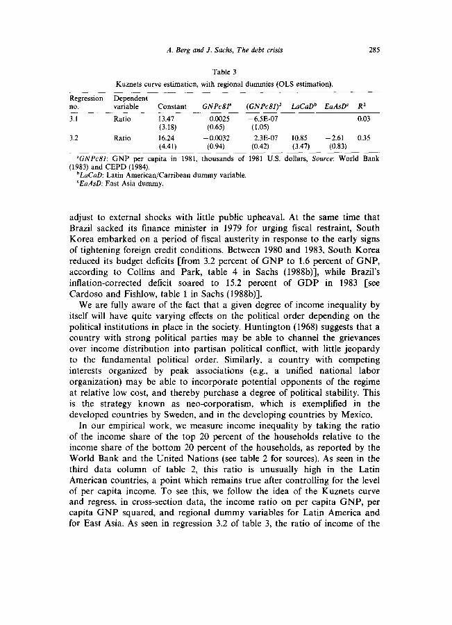
In our empirical work, we measure income inequality by taking the ratio of the income share of the top 20 percent of the households relative to the income share of the bottom 20 percent of the households, as reported by the World Bank and the United Nations (see table 2 for sources). As seen in the third data column of table 2, this ratio is unusually high in the Latin American countries, a point which remains true after controlling for the level of per capita income. To see this, we follow the idea of the Kuznets curve and regress, in cross-section data, the income ratio on per capita GNP, per capita GNP squared, and regional dummy variables for Latin America and for East Asia. As seen in regression 3.2 of table 3, the ratio of income of the
286 A. Berg and .I. Sachs, The debt crisis
top to the bottom 20 percent is significantly higher in Latin America than in East Asia. The ratio average 21.1 in Latin America (the per household income of the rich is 21.1 times greater than the per household income of the poor), and only 8.7 in East Asia.
We have restricted ourselves to income distribution data which in principle come from household surveys of the entire population, use a common unit (the household), and include income from all sources. This variable is measured with error, of course; we can only hope that the cross-country variation will dominate measurement error. For a discussion of the sources and quality of this data, see for example Jain (1975).
A second indicator of political stability that we investigate is the share of the national production that is located in the agricultural sector, as reported in the fifth data column in table 2. The share of agriculture in production is included to offer a rough indication of the extent to which governments can derive their political backing from rural interests rather than urban interests, on the theory that a rural power base tends to be more stable and more supportive of export-promoting policies.
We have already touched on Huntington’s analysis of the links between a rural base of power and political instability. Mobilized opposition to the government tends to be found in the urban centers, where students, government works, industrial workers, and so on, can be successfully organized. Not only can these groups threaten the survival of a regime, they can also apply effective pressure for government spending and low taxes on the urban population as the price for political peace. There may also be a direct link between agriculture and trade policy: in most countries agriculture is a tradeable good that is hurt by an overvalued exchange rate and by a heavy emphasis on import-substitution policies.
These ideas find initial support in our sample of countries. It is noteworthy that among the 35 countries that we are considering, the incidence of violent coups in the 1970s can be partially explained in a probit model as a negative function of the share of agriculture in GNP during the decade, controlling for the level of per capita income (higher income countries, ceteris paribus, showed a smaller probability of a violent COUP).~ To see why this relationship is found, note that of the 15 countries in the sample with a share of agriculture in GNP of 15 percent or less, six countries (40 percent) experienced a violent coup during the 1970s. Of the eleven countries with a
6The probit regression takes the form
COUP7080=2.01-0.115 * AGV 7081- 1.4E-7 *(GNPc81)‘, (1.78) (2.34) (1.84)
where 80% of the countries are correctly predicted and t-statistics are in parentheses. COUP7080 is a dummy variable which takes a 1 if there was a coup during the 1970s for that particular country and 0 otherwise.
A. Berg and J. Sachs, The debt crisis 287
share of agriculture in GNP of 25 percent or more, only Thailand (nine percent of the cases) experienced a violent coup.’
In our view, it is the importance of the rural base of politics that helps to explain why Colombia is the only commercial borrower in Latin America to have escaped a debt crisis in the 1980s. Colombia’s share of agriculture in GNP averaged 29 percent during 197Sl981, which was by far the highest for the region, and more than twice the overall average for Latin America and the Caribbean, 12.1 percent of GNP. It has been suggested by some observers that the heavy political influence of the coffee growers in Colombia contributed importantly to the government’s decision to introduce the crawling-peg exchange rate in 1967, a policy innovation which has been instrumental in the past two decades in permitting Colombia to avoid the worst ravages of currency overvaluation.
Along a similar line, Urritia [in Sachs (1988a)] explains Colombia’s relative fiscal prudence during the 1970s according to the unusual structure of its politics:
Finally, the government in 19741978 had a large rural base of support, and the President had developed a strong commitment to promoting development in the rural sector and dismantling the import substitution model of development. He was against subsidizing organized labor and industrialists, was anti-bureaucracy, and had his urban support among the unorganized who suffered most from inflation.. . . The main objective of the government in power between 1974 and 1978 was to control inflation, and with this objective, it carried out a tax reform in 1974, and also to control inflation, the government did not increase the foreign debt.
In contrast, in the early eighties, another government, whose political base was largely the bureaucracy, increased debt and government expenditure rapidly. That policy created a mini-debt crisis in 1983-1984, but Colombia was the only country in Latin America that adjusted successfully after 1982. It did it by almost wiping out the fiscal deficit in 1984-1985, not only by decreasing expenditures, but also by increasing taxation.
3. Empirical implementation of the probability model
We now turn to the empirical implementation of the probability models. We run two basic equations: a probit model that estimates a probability function for reschedulings with commercial creditors, and a tobit model that
‘The countries with at least one violent coup in the 1970s are: Argentina, Chile, Ecuador, Peru, Thailand, Portugal, and Turkey.
288 A. Berg and .I. Sachs, The debt crisis
estimates the size of the discounts on borrowing country debt sold in the secondary markets. For each model, we use two distinct samples: a sample of the 24 countries for which the World Bank’s outward-orientation variable is available, and a more inclusive sample of 35 commercial borrowers.
In order to include the outward-orientation variable in the large sample, we follow a standard procedure [see for example Maddala (1977)]. In a tirst- stage regression, we regress the outward-orientation measure on the other right-hand side variables in our sample of 24 countries. Using the estimated coefficients, we then create a fitted measure of outward orientation for the 11 missing countries, by applying the regression coefficients to the right-hand side values for the 11 countries. The new synthetic outward-orientation variable now has 35 observations, the 24 original observations and 11 fitted values.8
The basic probit model attempts to explain the pattern of reschedulings and non-reschedulings according to four variables: the income distribution (ratio of household income of top 20 percentiles over bottom 20 percentiles, RATIO), outward orientation of policies during 1973-1985 (OUT7385), the share of agriculture in GNP during 1970-1981 (AGu7081), and the level of per capita GNP (in %U.S.) in 1981 (GNPc81). The last variable is included for several reasons. First, higher-income countries may be less likely to reschedule than poorer countries since the costs of rescheduling (a loss of access to new lending on normal market terms, a partial disruption of normal trade relations, IMF surveillance, and so forth) would tend to be more onerous for more advanced economics. Second, the high levels of per capita income may reflect other characteristics of a country that would tend to reduce the chances for debt rescheduling, e.g., more effective economic and political institutions (controlling for income distribution, agricultural share of GNP, etc.). Third, the other explanatory variables are also known to be a function of per capita GNP. It is thus especially important to verify that income distribution and the agricultural share are not simply proxying for the level of economic development, but are indeed reflecting a deeper structural feature of the economy.
In most of the regressions that follow, GNP per capita is actually entered as GNP per capita squared, since some preliminary regressions indicated that
8This procedure will improve the efficiency of estimation in that it allows us to use a larger sample of data. However, the use of the estimated explanatory variable will introduce heteroskedasticity as well as additional small sample bias. The net effect is uncertain. Furthermore the t-statistics shown in the paper are calculated as if the estimated values were the true ones. They should probably be corrected for degrees of freedom, although of course these tests are only asymptotically valid anyway. Finally, this procedure is consistent only for linear estimation, since the expectation of a non-linear function is not equal to the function evaluated at the expectation of its arguments. However, to make a careful correction for this problem would require very special assumptions about the distributions. All this should serve to emphasize that our econometric results are designed primarily to be descriptive of the data, not rigorous statistical tests.
A. Berg and J. Sachs, The debt crisis 289
the non-linear specification slightly improves the performance of the model. The variable always enters with a negative sign, suggesting that indeed higher income countries are less likely to reschedule than poorer countries. Since the variable enters best as a squared term, we find that the very high income countries in our sample are considerably less likely to reschedule than the poorer countries. Indeed, none of the countries with a per capita income above $5,000 actually reschedules. Venezuela, at $4,220 per capita, is the country with the highest per capita income to reschedule.
The probit equation for the sample of 24 countries proves to be an embarrassment of riches. Specifically, the four variables in the model perfectly discriminate among the reschedulers versus the non-reschedulers. What this means is that there exists a linear combination of the right-hand side variables such that a rescheduling probability of less than 0.5 is assigned by the probit model for all countries that do not reschedule, and a probability of greater than 0.5 is assigned for all countries that do reschedule. Suppose that fi is an estimated vector of coefficients with that property (technically, Zfi is greater than 0.5 if and only if R, = 1). Then, any multiple of p, u * B for u> 1, will also perfectly discriminate among the reschedulers. Indeed, higher and higher values of u will raise the estimated likelihood function, since higher v will assign probabilities closer to 1.0 for countries that actually reschedule, and 0.0 for countries that do not.
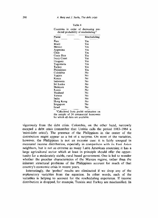
The upshot of all of this is that because of the small sample, and the ‘perfect’ tit, we cannot actually estimate coefficients and standard errors for the probit equation. We can, however, get an ordinal ranking of the probabilities of rescheduling from ‘most likely’ to reschedule to ‘least likely’ to reschedule. This list is shown in table 4. As advertised, the equation perfectly orders the countries: those that are ‘most likely’ to have rescheduled are exactly those at the top of the list, and those ‘least likely’ are on the bottom.
The list itself is extremely illuminating. The ‘worst’ case is Peru. It is has a highly unequal income distribution, a low share of agriculture in GNP, a low per capita income, and an inward-oriented trade policy. It is perhaps not surprising then that Peru’s debt is also the lowest valued of all the commercial borrower debt on the secondary market as of the end of 1987. For all of the reasons that Peru is likely to have rescheduled, Israel escaped rescheduling: the income distribution is quite equal, the agricultural share in GNP is large, per capita income is large, and trade policy is outward oriented. Looking at the ranking of countries, it is evident that the Latin American countries rank near the very top (with the exception of Colombia), while the East Asian economies are near the bottom.
The ‘hard’ cases are the countries like Turkey, Tunisia, Philippines, and Colombia, which fall in the middle of the probability distribution. Interest- ingly, Turkey is probably the rescheduling country that has recovered most
290 A. Berg and J. Sachs, The debt crisis
Table 4
Countries in order of decreasing pre- dicted probability of rescheduling.”
Name Rescheduling
Peru Brazil Mexico Argentina Chile Costa Rica Ivory Coast Uruguay Yugoslavia Turkey Philippines Colombia Tunisia Kenya Indonesia Sri Lanka Malaysia Korea Thailand Taiwan India Hong Kong Singapore Israel
Yes Yes Yes Yes Yes Yes Yes Yes Yes Yes Yes No No No No No No No No No No No No No
“Calculated from probit estimation on the sample of 24 commercial borrowers for which all data are available.
vigorously from the debt crisis. Colombia, on the other hand, narrowly escaped a debt crisis (remember that Urritia calls the period 1983-1984 a ‘mini-debt crisis’). The presence of the Philippines in the center of the distribution might appear as a bit of a surprise. On most of the variables, however, the Philippines is not an extreme case: it is fairly unequal in measured income distribution, especially in comparison with its East Asian neighbors, but is not as extreme as many Latin American countries; it has a large agricultural sector which at least in principle should offer the oppor- tunity for a moderately stable, rural based government. One is led to wonder whether the peculiar characteristics of the Marcos regime, rather than the inherent structural problems of the Philippines account for much of that country’s economic crisis in recent years.
Interestingly, the ‘perfect’ results are eliminated if we drop any of the explanatory variables from the equation. In other words, each of the variables is helping to account for the rescheduling experience. If income distribution is dropped, for example, Tunisia and Turkey are misclassified. In
A. Berg and J. Sachs, The debt crisis 291
Table 5
Probit 6.1 with omitted variables.
Omitted variable
Predicted to reschedule
Predicted not to reschedule
RATIO Tunisia Turkey
AGV 7081 Colombia Chile India Uruguay Kenya Yugoslavia
OUT 7385 Tunisia Philippines
GNPc81 Colombia Philippines Israel Turkey
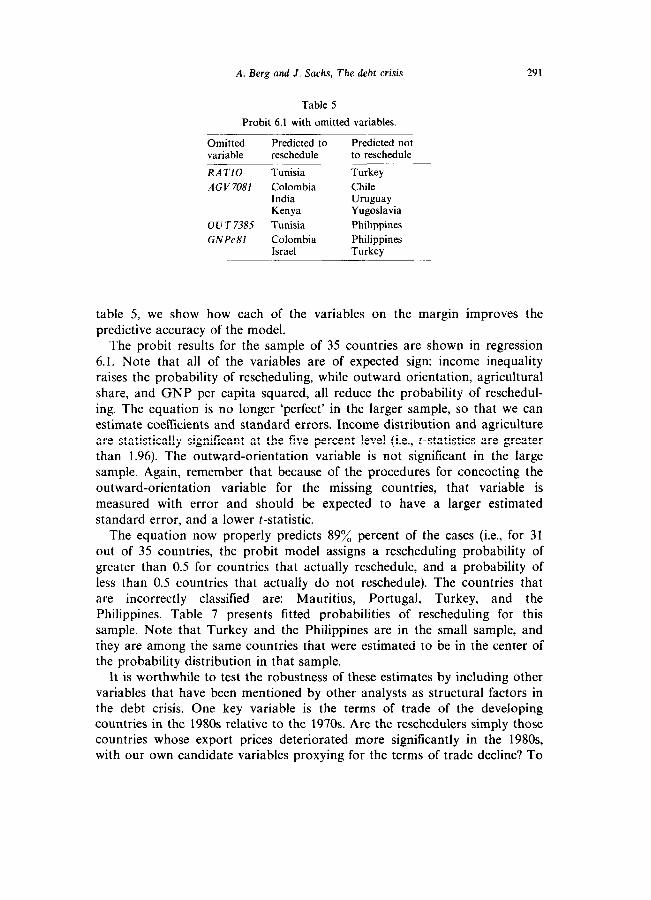
table 5, we show how each of the variables on the margin improves the predictive accuracy of the model.
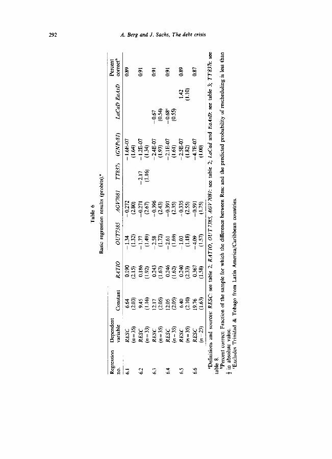
The probit results for the sample of 35 countries are shown in regression 6.1. Note that all of the variables are of expected sign: income inequality raises the probability of rescheduling, while outward orientation, agricultural share, and GNP per capita squared, all reduce the probability of reschedul- ing. The equation is no longer ‘perfect’ in the larger sample, so that we can estimate coefficients and standard errors. Income distribution and agriculture are statistically significant at the five percent level (i.e., c-statistics are greater than 1.96). The outward-orientation variable is not significant in the large sample. Again, remember that because of the procedures for concocting the outward-orientation variable for the missing countries, that variable is measured with error and should be expected to have a larger estimated standard error, and a lower t-statistic.
The equation now properly predicts 89% percent of the cases (i.e., for 31 out of 35 countries, the probit model assigns a rescheduling probability of greater than 0.5 for countries that actually reschedule, and a probability of less than 0.5 countries that actually do not reschedule). The countries that are incorrectly classified are: Mauritius, Portugal, Turkey, and the Philippines. Table 7 presents fitted probabilities of rescheduling for this sample. Note that Turkey and the Philippines are in the small sample, and they are among the same countries that were estimated to be in the center of the probability distribution in that sample.
It is worthwhile to test the robustness of these estimates by including other variables that have been mentioned by other analysts as structural factors in the debt crisis. One key variable is the terms of trade of the developing countries in the 1980s relative to the 1970s. Are the reschedulers simply those countries whose export prices deteriorated more significantly in the 198Os, with our own candidate variables proxying for the terms of trade decline? To
Tab
le
6
Bas
ic
regr
essi
on
resu
lts
(pro
bits
).”
Reg
ress
ion
Dep
ende
nt
Perc
ent
no.
vari
able
C
onst
ant
RA
TIO
O
UT
7385
A
GV
7081
T
T83
7s
(GN
P&)
LaC
aD
EaA
sD
corr
ectb
6.1
RE
SC
6.64
0.
190
- 1.
34
-0.2
12
- -
1.6E
-07
0.89
(n
=35)
(2
.03)
(2
.15)
(1
.32)
(2
.80)
(1
.64)
6.2
RE
SC
9.45
0.
186
-1.7
7 -0
.271
-2
.17
- 1.
2E-0
7 0.
91
(n=3
3)
(1.1
6)
(1.9
2)
( 1.4
9)
(2.6
7)
(1.1
6)
(1.3
4)
6.3
RE
SC
12.1
7 0.
243
- 2.
58
-0.3
96
- 2.
4E-0
1 -0
.67
0.91
(n
=35)
(2
.05)
(1
.67)
(1
.72)
(2
.43)
(1
.93)
(0
.54)
6.4
RE
SC
12.0
5 0.
246
-2.6
1 -0
.391
-2
.lE-0
7 -
0.68
’ 0.
91
(n=3
5)
(2.0
5)
(1.6
2)
(1.6
9)
(2.3
5)
(1.6
1)
(0.5
5)
6.5
RE
SC
6.40
0.
240
- 1.
03
-0.3
35
-2.5
E-0
7 1.
42
0.89
(n
=35)
(2
.10)
(2
.33)
(1
.18)
(2
.55)
(1
.82)
(1
.10)
6.6
RE
SC
19.7
6 0.
367
-4.0
9 -0
.591
-4
.lE-0
1 0.
87
(n=2
3)
(1.6
3)
(1.5
8)
(1.5
7)
(1.7
5)
(LO
O)
“Del
initi
ons
and
sour
ces:
R
ESC
: se
e ta
ble
2; R
AT
IO,
OU
T73
85
AG
V70
81:
see
tabl
e 2;
L&
ad
and
EaA
sD:
see
tabl
e 3;
T
T83
7s:
see
tabl
e 8.
‘P
erce
nt
corr
ect:
Frac
tion
of t
he
sam
ple
for
whi
ch
the
diff
eren
ce
betw
een
Res
t an
d th
e pr
edic
ted
prob
abili
ty
of r
esch
edul
ing
is l
ess
than
f
in
abso
lute
va
lue.
‘E
xclu
des
Tri
nida
d &
T
obag
o fr
om
Lat
in
Am
eric
a/C
arib
bean
co
untr
ies.

Name
Peru Ecuador Panama Brazil Argentina Mexico Chile Venezuela Ivory Coast Costa Rica Mauritius Morocco Uruguay Yugoslavia Portugal Colombia Turkey Philippines Kenya
Egypt Tunisia Hong Kong Hungary Malaysia Singapore Israel Trinidad & Tobago Indonesia Sri Lanka Thailand Korea India Taiwan China Spain
Fitted probability of rescheduling
l.oooooO 1S0OOOO l.OOOOOO 0.999998 0.999920 0.999690 0.951620 0.934080 0.933460 0.898180 0.886290 0.774910 0.728700 0.615020 0.537960 0.464500 0.399410 0.274890 0.116730 0.109160 0.088340 0.038940 0.021690 0.019490 0.013080 0.012420 0.011230 0.006740 0.004700 0.000450 0.000350 0.000150 0.000050 O.OOOOO6 o.OOOOO3
A. Berg and .I. Sachs, The debt crisis 293
Table 7
Comparison of fitted probability of rescheduling with actual event (from regression 6.2).
Rescheduler
Yes Yes Yes Yes Yes Yes Yes Yes Yes Yes No Yes Yes Yes No No Yes Yes No No No No No No No No No No No No No No No No No
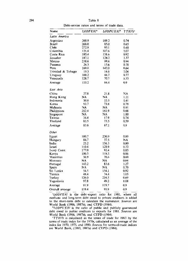
test this possibility, we include as a right-hand side variable the terms of trade of the countries in 1983 relative to an average terms of trade in the 1970s (measured as the simple average for 1970, 1975, and 1980). As seen in table 8, most of the countries experienced a terms of trade decline in the 1980s but there is little evidence that the extent of the terms-of-trade deterioration in fact played a major role in affecting which countries required rescheduling and which ones did not. Many oil exporters (e.g. Venezuela), for example, enjoyed a terms of trade improvement comparing the 1980s and the 1970s but in fact succumbed to rescheduling, while many oil importers (such
294
Name LODPX81’ LODPUX81b TT837s’
Table 8
Debt-service ratios and terms of trade data.
Latin America
Argentina Brazil Chile Colombia Costa Rica Ecuador Mexico Panama Peru Trinidad & Tobago Uruguay Venezuela
Average
East Asia
China Hong Kong Indonesia Korea Malaysia
Singapore Taiwan Thailand
Average
Other
Egypt Hungary India Israel Ivory Coast Kenya Mauritius Morocco Portugal Spain Sri Lanka Tunisia Turkey Yugoslavia
Average 91.9 0.9
Overall average 119.4 0.9
“LODPX81 is the debtexport ratio for 1981, where all medium- and long-term debt owed to private creditors is added to the short-term debt to calculate the numerator. Sources are World Bank (1986, 1987b), and CEPD (1984).
268.9 268.0 272.8 121.4 185.4 187.1 238.6
26.3 160.0
19.3 100.2 128.7
155.2
27.8 NA
50.8 93.7
NA 212.4 NA
34.4 82.5
83.6
100.7 84.7 23.2
110.4 177.0 loo.3
36.9 NA 143.2 NA
54.5 48.4
126.0 97.8
109.2 85.0 93.1
107.6 131.6 124.2 99.8 15.6
142.0 14.6 44.7 70.7
84.4
21.8 NA
53.5 73.8
NA 161.9 NA
17.9 73.5
67.1
230.9 37.5
156.3 128.9 92.4
118.5 76.6
NA 83.6
NA 154.1 74.4
234.5 49.2
119.7
95.9
0.74 0.65 0.48 1.07 0.92 1.37 0.94 0.78 0.64 1.04 0.77 1.53
0.9
NA 1.11 1.41 0.78 0.91 0.68 1.00 0.74 0.59
0.9
0.89 NA 0.80 0.73 0.85 0.86 0.60 0.64 1.27 0.70 0.92 1.05 0.69 1.08
bLODPUX81 is the ratio of public and publicly guaranteed debt owed to public creditors to exports for 1981. Sources are World Bank (1986, 1987b), and CEPD (1984).
“TT837s is calculated as the terms of trade for 1983 by the terms of trade index for the 1970s. calculated as an average of the index for 1970, 1975, and 1980. Sources for terms-of-trade indices are World Bank, (1983, 1987a) and CEPD (1984).
A. Berg and J. Sachs, The debt crisis 295
as Israel, Korea, Taiwan, and Thailand) suffered a sharp terms-of-trade deterioration without a rescheduling.
The probit model in the sample of 35 countries is estimated with the terms of trade in regression 6.2. The terms of trade is statistically insignificant, while the other variables maintain their earlier signs and approximate magnitudes. The variables for income distribution and agricultural shares remain significant. The weak finding on the terms of trade is consistent with earlier studies, particularly Sachs (1985) who showed that the differences in experiences of Latin American and East Asian economies could not be explained by differing patterns in the terms of trade.
Since most of the rescheduling countries are in Latin America, and since the Latin American economies are characterized by extremely unequal income distributions, it is important to check whether the income distri- bution variable is merely proxying for other characteristics of the Latin American economies (note that ten of the 12 economies in Latin America and the Caribbean reschedule, while only tive of the remaining 23 countries reschedule). In other words, is the income distribution effect truly structural, or is it merely a dummy variable for Latin America? To examine this question, we introduce in regressions 6.3 and 6.4 two alternative dummy variables for the region, depending on whether we count Trinidad and Tobago as part of Latin America. (If the idea of the dummy variable is to measure an effect specific to ‘Latin’ societies, Trinidad and Tobago should be excluded; if the idea is to capture a geographical effect in which the creditor banks redline the developing economies of the Western Hemisphere, then Trinidad and Tobago should be included in the dummy variable).
Rather remarkably, the both versions of the Latin American dummy variable are statistically insignificant, and while their introduction reduces the significance of income distribution, the magnitude of the coefficient on income distribution increases and the dummy variable for Latin America has the unexpected sign (lower probability of rescheduling, controlling for the other variables)! In other words, once our structural variables are included, the fact that a country is in Latin American does not seem to have raised the probability of rescheduling. It is also worthwhile to verify that the equation is not proxying for the East Asian economies. A dummy variable for East Asia also is insignificant, has less effect on the other variables [eq. (6.5)], and also has the unexpected sign. Adding both the Latin American and East Asian dummy variables yields similar results (not shown).
Another convincing way to verify that we are picking up something more than a ‘Latin’ effect in our regression model is to run the probit model for the non-Latin American sample. There are, of course, a very small number of countries that remain in the sample, but as seen in regression 6.6, all of the structural variables maintain their signs and increase in magnitude in the non-Latin sample of countries. Given the small size of the sample, the
296 A. Berg and .I. Sachs, The debt crisis
statistical significance of the explanatory variables is reduced, but the income distribution variable remains near the ten percent level of significance.
The next step in our investigation is to estimate a tobit model of the size of the discount on each country’s debt in the secondary market. The idea of the tobit model is as follows. We assume that the discount on the debt is a non-linear function of the explanatory variables that we have already introduced, with the non-linearity arising from the fact that the discount on the debt can be positive or zero, but never negative (the discount measures the percentage difference in the par value of the debt and the secondary market value). For a range of creditworthiness, the debt will sell at par, i.e., with a zero discount, If the creditworthiness falls below a certain threshold, then the discount on the debt becomes positive.
The specific model is as follows. Let DT be a latent creditworthiness variable for country i, that is a function of the explanatory variables Zi and a random error term ui distributed normally, so that
D* =ZiB + Vi,
where p is a vector of coefficients. Higher 0: signifies lower creditworthiness. For 0: less than or equal to zero, the actual discount Di is equal to zero, while for Df greater than zero, the actual discount Di is set equal to 0;. That is,
Di=O for D:<O,
=Dr for Dr>O. (4)
In general, 0: represents a threshold for rescheduling. For countries that have not rescheduled, the discount is zero (or very close to zero), while for countries that have rescheduled, the discount tends to be positive.
In practice, this last observation may be violated. For example, Colombian debt sold at a 40 percent discount at the end of 1987, despite the fact that Colombia never rescheduled. For most countries that have not rescheduled, the secondary market price of the debt is not publicly quoted (e.g., by the investment banks, that send newsletters on secondary market prices). For those countries, we assume in the tobit regressions that follow that the actual market discount is equal to zero. This is probably a good assumption, since if the country’s debt in fact traded at a discount, the secondary market price of the country’s debt would tend to be quoted.
It is our basic assumption that the variables that conduce to reschedulings are the same ones that lead to low secondary market prices for a country’s debt. This conclusion is borne out by the battery of tobit regressions reported in table 9. As usual, regression results are reported for samples of 24

Tab
le
9
Bas
ic
regr
essi
on
resu
lts
(tob
its).
” ~_
__~
Reg
ress
ion
Dep
ende
nt
no.
vari
able
C
onst
ant
RA
TIO
O
UT
7385
A
GV
7081
(G
NPc
81)’
L
.uC
aD
EaA
sD
TT
83 7
s
9.1
DIS
C
1.11
0.
012
-0.2
3 -
0.03
0 -
1.8E
-08
(n=3
5)
(4.4
3)
(2.6
1)
(3.1
3)
(4.2
1)
(1.8
0)
9.2
DIS
C
1.15
0.
014
-0.2
0 -0
.031
-
2.6E
-08
(n =
24)
(5
.43)
(2
.81)
(3
.53)
(5
.18)
(2
.12)
9.3
DIS
C
1.23
0.
011
-0.2
3 -
0.02
8 -
1.8E
-08
-0.1
5 (n
=
33)
(3.9
6)
(1.8
7)
(2.4
3)
(3.9
0)
(2.1
4)
(0.8
8)
9.4
DIS
C
4.19
0.
013
-0.2
0 -0
.031
-
2.6E
-08
- 0.
02
(n =
24)
(4
.19)
(2
.62)
(3
.50)
(4
.85)
(2
.08)
(0
.1 I
)
9.5
DIS
C
1.00
0.
007
-0.2
0 -
0.02
4 -
2.4E
-08
0.20
(n
=35)
(3
.74)
(1
.37)
(3
.10)
(3
.47)
(2
.67)
(1
.77)
9.6
DIS
C
0.94
0.
011
-0.1
8 -
0.02
4 -
2.2E
-08
0.15
(n
=
24)
(3.8
2)
(2.2
4)
(3.3
4)
(3.4
8)
(1.5
8)
(1.4
6)
9.7
DIS
C
0.92
0.
007
-0.2
0 -
0.22
0 -
1.9E
-08
0.20
b (n
=35)
(3
.53)
(1
.45)
(3
.16)
(3
.20)
(1
.89)
(1
.84)
9.8
DIS
C
1.07
0.
014
-0.2
3 -0
.036
-2
.lE-0
8 0.
044
(n=3
5)
(4.2
0)
(2.9
5)
(2.8
6)
(4.0
6)
(2.0
2)
(0.3
1)
9.9
DIS
C
1.15
0.
014
-0.0
2 -0
.031
-
2.6E
-08
0.00
3 (n
= 2
4)
(5.4
3)
(2.7
4)
(3.4
6)
(5.0
7)
(2.1
3)
(0.0
3)
“Def
initi
ons
and
sour
ces:
D
ISC
: se
e ta
ble
1;
RA
TIO
, O
UT
7385
, A
GV
7081
: se
e ta
ble
2;
LaC
aD
and
EuA
sD:
see
tabl
e 3;
T
T83
7s:
see
tab
le
8.
%ig
niIi
es
the
excl
usio
n of
T
rini
dad
&
Tob
ago
from
th
e co
untr
ies
desi
gnat
ed
to
be
Lat
in
Am
eric
an.

298 A. Berg and J. Sachs, The debt crisis
Table 10
Fitted and actual discounts from regression 9.2.
Discount
Name Fitted Actual Residual
Argentina Brazil Chile Colombia Costa Rica Ivory Coast Mexico Peru Philippines Uruguay Yugoslavia
0.63 0.47 0.30 0.10 0.29 0.25 0.53 1.05 0.12 0.17 0.22
0.53 -0.10 0.45 -0.02 0.33 0.03 0.19 0.09 0.67 0.38 0.40 0.15 0.47 -0.06 0.89 -0.16 0.33 0.21 0.32 0.15 0.30 0.08
and 35. In both cases, the income distribution variable is always positive (higher inequality leads to a greater discount on the debt), while the outward-orientation variable, the agricultural share variable, and GNP per capita squared, are always negative (higher values tend to decrease the secondary market discount). In most regressions, all of the explanatory variables are statistically significant.
Consider the basic regression over the sample of 24 countries, reported as regression 9.1. For those countries with a reported secondary market discount, the actual and fitted values of the debt are reported in table 10. Note that among countries with a discount on the debt, Peru has the largest fitted discount, and the largest discount actually reported in the data, while the fitted discount on Colombia is the lowest among the countries with a positive discount. It is instructive to consider the sources of the fitted discount on Peru as compared with the fitted discount on a hypothetical average East Asian country. Peru’s fitted discount is actually above 100 percent, at 105 percent, versus the discount of about -2 percent for ‘East Asia’.9 Of this difference of 197 percentage points, 31 can be attributed to Peru’s worse income distribution; another 31 can be attributed to the lower level of agriculture in Peru; another 44 can be attributed to the greater outward orientation of ‘East Asia’; and, finally, a negligible amount can be attributed to Peru’s lower level of per capita income.
The tobit model is also an appropriate model for testing the role of terms of trade shocks, and dummy variables for Latin America and East Asia.
9The ‘predicted discount’ cannot actually be negative, of course, but the prediction for the average of the region is near enough to zero that no great violation is committed.
A. Berg and J. Sachs, The debt crisis 299
Various results are reported in table 9. We find that the terms of trade has even less effect in accounting for the size of the discount on the debt. While the dummy variables for Latin America and East Asia are always small and insignificant once we control for the structural variables in our model, the Latin American dummy variable does have more power than in the probit regressions.
Many earlier studies have shown that the probability of debt rescheduling is a positive function of the debt-export ratio. It is therefore worthwhile to ask whether our variables help to account for the debt&export ratio, or whether our variables work through some alternative mechanism (in which case the debtexport ratio might be an additional explanatory variable). We conclude this section by examining this issue. (Table 8 presents the debt- export ratio data.)
As shown by regressions 11.1 and 11.2, in table 11, it is the debt owed to private creditors rather than public creditors that poses the greatest risk of forcing the country into a rescheduling or reducing the secondary market value of the country’s debt (not shown). Note for example that the ratio of debt to private creditors relative to exports is a highly significant predictor of reschedulings, while the debt owed to foreign official creditors, as a proportion of exports, does not help to explain reschedulings and even has the wrong sign. The relative importance of debts to private creditors rather than official creditors reflects the fact that the interest rates on most of the private debt were set on a variable rate basis, and thus rose sharply when U.S. interest rates increased after 1979. The interest rates on debts owed to official creditors rose far more slowly in the early 1980s.
According to regression 11.4, our set of explanatory variables accounts well for the cross-country differences in debt-export ratios (note that we now restrict our attention to debt owed to private creditors). As per our earlier political arguments, higher income inequality and a lower argicultural share in GNP are associated with higher levels of debt relative to exports. The relationship is not particularly robust, however, since the statistical signifi- cance of the link between income distribution and the debtexport ratio disappears when we move from the small sample of countries to the larger sample (regression 11.3).
According to the probit and tobit equations in regressions 11.5-11.7, the effects of income distribution, agriculture, and outward orientation on the probability of rescheduling and the discount on the debt are fairly strongly mediated by the debt&export ratio. Even after controlling for the debt&export ratio, the key variable of our model remain significant in the tobit analysis. The debt&export ratio itself is statistically significant once there other variables are included in the regressions. Thus, while high income inequality tends to raise the country’s debtexport ratio, it also seems to reduce the country’s capacity to deal with any particular level of the debt. Given this,
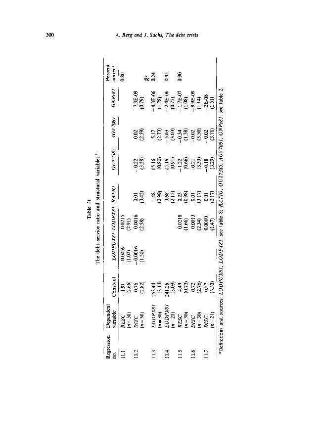
Tab
le
11
The
de
bt-s
ervi
ce
ratio
an
d st
ruct
ural
va
riab
les.
”
Reg
ress
ion
no.
11.1
11.2
11.3
11.4
II.5
11.6
11.7
Dep
ende
nt
vari
able
RE
SC
(n=
30
)
DIS
C
(n=
30)
LO
DP
XB
I (n
= 3
0)
LO
DP
Xll
I (n
=21)
RE
SC
(n=
30)
DIS
C
(n=
30
)
DIS
C
(n=2
1)
Con
stan
t
- 1.
91
(2.6
6)
0.76
(2
.82)
253.
44
(3.1
4)
241.
26
(3.0
9)
4.49
(0
.73)
0.72
(2
.76)
0.87
(3
.33)
LO
DP
UX
BI
LO
DP
XB
I R
AT
IO
- 0.
0059
0.
0215
(1
.02)
(2
.91)
-0.0
016
0.00
16
0.01
(1
.50)
(2
.58)
(3
.42)
1.48
(0
.99)
3.68
(2
.15)
0.02
18
0.23
(1
.66)
(0
.98)
0.00
13
0.01
(2
.34)
(3
.17)
0.00
10
0.01
(1
.47)
(2
.17)
OU
T73
85
-0.2
2 (3
.28)
-15.
16
(0.8
0)
- 15
.16
(0.9
1)
- 1.
22
(0.6
6)
-0.2
1 (3
.33)
-0.1
8 (3
.29)
AG
V70
81
GN
P&
I
corr
ect
- 0.
02
(2.5
9)
-5.1
7 (2
.73)
- 5.
63
(3.0
3)
-0.3
4 (1
.38)
- 0.
02
(3.5
0)
- 0.
02
(3.7
1)
0.80
-7.3
E-0
9 (0
.79)
82
-4
.3E
-06
0.24
(1
.78)
- 2.
4E-0
6 0.
45
(0.7
5)
- 1.
7E-0
7 0.
90
(1.0
8)
- 9.
9E-0
9 (1
.14)
- 2E
-08
(1.5
1)
“Def
initi
ons
and
sour
ces:
L
OD
PU
XSI
, L
OD
PX
8I:
see
tabl
e 8;
R
AT
IO,
OC
U73
85,
AG
V70
81,
GN
P&
I:
see
tabl
e 2.
A. Berg and J. Sachs, The debt crisis 301
however, the level of the debt-export ratio seems to have some independent effect.
4. Additional variables in the probability model
There are many additional variables that have been suggested in the literature as having played a role in the debt crisis. To our rather considerable surprise, most of the variables had little explanatory power in the probit and tobit equations either by themselves or in conjunction with our other variables. We examined, without success, the following variables for a possible contribution to our models:
- the share of manufacturing exports in total exports (expected to reduce the probability of rescheduling);
- the share of fuels, mineral, and metals in total exports (expected to raise the probability of rescheduling);
- the rate of population growth between 1970-1985; _ the size of the population in 1981; _ the commodity concentration of exports (expected to raise the probability
of rescheduling, because of increased vulnerability to terms of trade shocks, and increased difficulty in short-term export promotion);
_ the rate of national savings (expected to lower the probability of rescheduling).
Only the last two variables came at all close to adding to the explanatory power of the model, but neither variable reached statistical significance.*O The regressions with the additional variables are reported in table 12, the data in table 13.
5. Towards an interpretation of the linkage of economic inequality and foreign debt management
We have identified four key structural variables that help us to explain which of the developing countries succumbed to debt crises in the 198Os, and we have suggested some of the linkages between the structural variables and the outcomes of debt management. In this section we discuss further the possible linkages between income inequality and the quality of debt management.
In terms of formal empirical analysis, we have so far made little headway
loThe share of fuels, minerals, and metals in total exports came in significantly in the smaller sample, but with a negative sign (a larger share reduced the predicted probability of rescheduling).
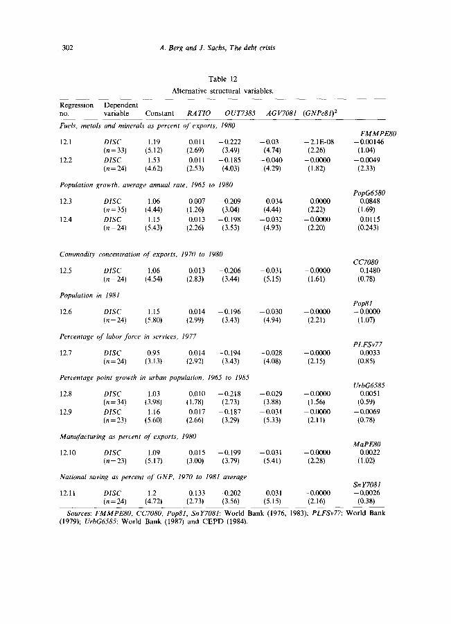
302 A. Berg and J. Sachs, The debt crisis
Table 12
Alternative structural variables.
Regression Dependent no. variable Constant RA TIO OUT7385 AGV7081 (GNPc81)=
Fuels. metals and minerals as percent of exports, 1980
12.1 DISC 1.19 0.011 - 0.222 (n=33) (5.12) (2.69) (3.49)
12.2 DISC 1.53 0.011 -0.185 (n=24) (4.62) (2.53) (4.03)
Population growth, average annual rate, 1965 to 1980
12.3 DISC 1.06 0.007 - 0.209 (n=35) (4.44) (1.26) (3.04)
12.4 DISC 1.15 0.013 -0.198 (n = 24) (5.43) (2.26) (3.53)
Commodity concentration of exports, 1970 IO 1980
12.5 DISC 1.06 0.013 - 0.206 (n = 24) (4.54) (2.83) (3.44)
Population in 1981
12.6 DISC 1.15 0.014 -0.196 (n = 24) (5.80) (2.99) (3.43)
Percentage qf labor ,force in services. 1977
12.7 DISC 0.95 0.014 -0.194 (n = 24) (3.13) (2.92) (3.43)
Percentage point growth in urban population, 1965 to 1985
12.8 DISC 1.03 0.010 -0.218 (n= 34) (3.98) (1.78) (2.73)
12.9 DISC 1.16 0.017 -0.187 (n=23) (5.60) (2.66) (3.29)
Manufacturing as percent of exports. 1980
12.10 DISC 1.09 0.015 -0.199 (n=23) (5.17) (3.00) (3.79)
National saving as percent of GNP, 1970 to 1981 average
12.11 DISC 1.2 0.133 - 0.202 (n=24) (4.72) (2.73) (3.56)
- 0.03 (4.74)
-0.040 (4.29)
- 0.034
(4.44) -0.032
(4.93)
-0.031 (5.15)
- 0.030 (4.94)
- 0.028 (4.08)
- 0.029 (3.88)
-0.031 (5.33)
-0.031 (5.41)
-0.031 (5.15)
-2.lE-08 (2.26)
-0.0000 (1.82)
-O.oooO (2.22)
-O.OMXl (2.20)
-0.0000 (1.61)
-0.0000 (2.21)
-0.0000 (2.15)
-0.0000 (1.56)
-0.0000 (2.11)
-0.0000 (2.28)
-0.0000 (2.16)
FMMPE80 -0.00146
(1.04) -0.0049
(2.33)
PopG6580 0.0848
(1.69)
0.0115 (0.243)
CC7080 0.1480
(0.78)
Pop81 -0.0000
(1.07)
PLFSv77 0.0033
(0.85)
UrbG6585 0.0051
(0.59)
- 0.0069 (0.78)
MaPE80 0.0022
(1.02)
Sn I’7081 - 0.0026
(0.38)
Sources: FMMPWO, CC7080, Pop81, SnY7081: World Bank (1976, 1983); PLFSv77: World Bank (1979); UrbG6.585: World Bank (1987) and CEPD (1984).
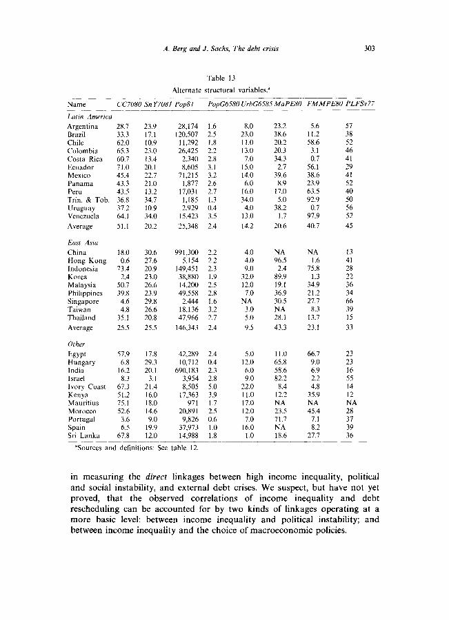
303 A. Berg and J. Sachs, The debt crisis
Name
Table 13
Alternate structural variables.” ~___.
CC7080 sn Y7081 Pop81 PopG6580 UrbG6585 MaPE80 FMMPEBO PLFSv77
Latin America
Argentina 28.7 Brazil 33.3 Chile 62.0 Colombia 65.3 Costa Rica 60.7 Ecuador 71.0 Mexico 45.4 Panama 43.3 Peru 43.5 Trin. & Tob. 36.8 Uruguay 37.2 Venezuela 64.1
Average 51.1
East Asia
China 18.0 Hong Kong 0.6 Indonesia 73.4 Korea 2.4 Malaysia 50.1 Philippines 39.8 Singapore 4.6 Taiwan 4.8 Thailand 35.1
Average 25.5
Other
Egypt Hungary India Israel
57.9 6.8
16.2 8.3
Ivory Coast 67.3 Kenva 51.2 Mauritius 15.1 Morocco 52.6 Portugal 3.6 Spain 6.5 Sri Lanka 67.8
23.9 28,174 1.6 8.0 23.2 5.6 57 17.1 120,507 2.5 23.0 38.6 11.2 38 IO.9 11,292 I.8 11.0 20.2 58.6 52 23.0 26,425 2.2 13.0 20.3 3.1 46 13.4 2,340 2.8 7.0 34.3 0.7 41 20.1 8,605 3.1 15.0 2.7 56.1 29 22.7 71,215 3.2 14.0 39.6 38.6 41 21.0 1,877 2.6 6.0 8.9 23.9 52 13.2 17,031 2.7 16.0 17.0 63.5 40 34.7 1,185 I.3 34.0 5.0 92.9 50 10.9 2,929 0.4 4.0 38.2 0.7 56 34.0 15,423 3.5 13.0 1.7 97.9 52
20.2 25,348 2.4 14.2 20.6 40.7 45
30.6 991,300 2.2 4.0 NA NA 13 21.6 5.154 2.2 4.0 96.5 1.6 41 20.9 149,451 2.3 9.0 2.4 75.8 28 23.0 38,880 1.9 32.0 89.9 1.3 22 26.6 14,200 2.5 12.0 19.1 34.9 36 23.9 49,558 2.8 7.0 36.9 21.2 34 29.8 2,444 I.6 NA 30.5 27.7 66 26.6 18,136 3.2 3.0 NA 8.3 39 20.8 41.966 2.7 5.0 28.1 13.7 15
25.5 146,343 2.4 9.5 43.3 23.1 33
17.8 42,289 2.4 5.0 11.0 66.7 23 29.3 10,712 0.4 12.0 65.8 9.0 23 20.1 690,183 2.3 6.0 58.6 6.9 16
3.1 3,954 2.8 9.0 82.2 2.2 55 21.4 8,505 5.0 22.0 8.4 4.8 I4 16.0 17,363 3.9 II.0 12.2 35.9 12 18.0 971 1.7 17.0 NA NA NA 14.6 20,891 2.5 12.0 23.5 45.4 28 9.0 9,826 0.6 7.0 71.7 7.1 37
19.9 37,973 1.0 16.0 NA 8.2 39 12.0 14.988 1.8 1.0 18.6 27.7 36
“Sources and definitions: See table 12.
in measuring the direct linkages between high income inequality, political and social instability, and external debt crises. We suspect, but have not yet proved, that the observed correlations of income inequality and debt rescheduling can be accounted for by two kinds of linkages operating at a more basic level: between income inequality and political instability; and between income inequality and the choice of macroeconomic policies.
304 A. Berg and J. Sachs, The debt crisis
We have pointed out that income inequality is likely to affect political stability in several different ways, making a test of the role of income inequality for political stability exceedingly difficult to quantify. In some countries, the income gap between strongly competing social groups may lead to a coup (as in many Latin American countries, when the government has been captured by populist forces); in other cases, the same kind of competition may lead to a fruitless and debilitating alternation of power between populists and orthodox politicians. In still other cases, a government may be able to hold on to power for a considerable period but only by ‘bribing’ the organized opposition, at the expense of fiscal discipline.
Through these effects, and others as well, we suspect that high income inequality hinders the adoption of needed policy changes on a timely basis. The basic decisions to liberalize trade or to cut budget deficits become too risky to bear in an environment of high income inequality. With regard to trade policy, for example, the shift away from inward-oriented growth towards outward-oriented growth seems to require an initial large real devaluation and sharp reduction in real wages, demonstrated by several historical examples: Korea in the early 1960s Brazil in the mid-1960s Chile in the 197Os, and Turkey in the early 1980s. It may be the case that income inequality must be sufficiently modest at the beginning of such experiments in order to carry out and sustain politically a major change of this sort.”
Similarly, the maintenance of realistic exchange rates and balanced budgets is probably more dillicult the greater is the income inequality. Unfortunately, because of the absence of good cross-country data on budget deficits we have not yet made any formal tests of the links of income inequality and budget deficits. It is our intention to piece together better data on a country-by- country basis as a prelude to such a test.12
Our analysis remains much too sketchy to draw any strong policy implications from our findings. The evidence presented in this paper says little about how to adapt policy recommendations to the political constraints that arise from the structural factors we have discussed. If the causal mechanisms we discuss are important, however, then successful policies, in particular successful stabilization and structural adjustment programs, will take into account distributional consequences.
While the evidence suggests that low income inequality is a precious asset for any economy, we have not yet investigated the efficacy of different kinds
“It is our guess that at least some of the staying power of the outward-orientation model in East Asia results from the relative equalities of income in the region. In Latin America, shifts in the trade regime towards outward orientation have been tried many times, and have repeatedly failed, under the weight of political protest by aggrieved workers.
‘*Similarly, measures of fundamental exchange rate misalignment, such as those presented in Edwards (1988), might allow a direct test of the importance of exchange rate misalignment and its relation to our structural variables.
A. Berg and J. Sachs, The debt crisis 305
of redistributive policies as ways to enhance the long-term political stability, and the effectiveness of economic management, in developing countries. In the absence of an improved distribution of income, however, we might pessimistically conclude that many Latin American economies will be faced with continuing cycles of political and economic instability.
References
Adelman, Irma and Sherman Robinson, 1987, Income distribution and development: A survey, in: H.B. Chenery and T.N. Srinivasan, eds., Handbook of development economics (North- Holland, Amsterdam).
Alesina, Albert0 and Guido Tabellini, 1987, External debts, capital flight, and political risk, Unpublished manuscript.
Balassa, Bela, 1982, Structural adjustment policies in developing countries, World Development 10, Jan., 23-38.
Balassa, Bela, 1984, Adjustment policies in developing countries: A reassessment, World Development 12, Sept., 955-972.
Bradford, Cohn, 1987, The NICs and the next-tier NICs as transitional economies, in: C. Bradford and W. Branson, eds., Trade and structural change in Pacific Asia (Chicago University Press, Chicago, IL).
Callier, Philippe, 1985, Further results on countries’ debt-service performance: The relevance of structural factors, Weltwirtschaftliches Archiv 121, 105-l 15.
Cline, William, 1984, International debt: Systemic risk and policy response (Institute of International Economics, Washington, DC) July.
Council for Economic Planning and Development (CEPD), Various years, Taiwan statistical data book (CEPD, Taipei).
Dornbusch, Rudiger and Y.C. Park, 1987, Korean growth policy, Brookings Papers on Economic Activity 2, 389454.
Edwards, Sebastian, 1988, Real and monetary determinants of real exchange rate behavior, theory and evidence from developing countries, Journal of Development Economics, this issue.
Feder, Gershon and Richard Just, 1977, A study of debt-servicing capacity applying logit analysis, Journal of Development Economics 4, no. 1, March.
Huizinga, Harry and J. Sachs, 1987, U.S. commercial banks and the developing country debt crisis, Working paper no. 2455 (National Bureau of Economic Research, Cambridge, MA) Dec.
Huntington, Samuel, 1968, Political order in changing societies (Yale University Press, New Haven, CT).
Jain, Shail, 1975, The size distribution of income: A compilation of data (The World Bank, Washington, DC).
Jodice, D.A. and C. Taylor, 1983, World handbook of political and social indicators, 3rd edition (Yale University Press, New Haven, CT).
Krueger, Anne O., 1978, Foreign trade regimes and economic development: Liberalization attempts and consequences (Ballinger, Cambridge, MA).
Kuznets, Simon, 1955, Economic growth and income inequality, American Economic Review 45, no. 1, l-28.
Lin, Ching-yuan, 1985, Latin America and East Asia: A comparative development perspective, Unpublished manuscript (International Monetary Fund, Washington, DC).
Little, Ian M.D., M. Scott and T. Scitovsky, 1970, Industry and trade in some developing countries (Oxford University Press, Oxford).
Maddala, G.S., 1977, Econometrics (McGraw-Hill, New York). McFadden, Daniel, R. Eckhaus, G. Feder, V. Hajivassihou and S. O’Connell, 1985, in: J.
Cuddington and G.W. Smith, eds., International debt and the developing countries (The World Bank, Washington, DC).
306 A. Berg and J. Sachs, The debt crisis
Pyo, Hak-Kil, 1987, External dependence and economic growth: An empirical inquiry, in K.D. Kim, ed., Dependency issues in Korean development (Seoul National University, Seoul).
Sachs, Jeffrey, 1985, External debt and macroeconomic performance in Latin America and East Asia, Brookings Papers on Economic Activity 2, 523-573.
Sachs, Jeffrey, 1987, Trade and exchange rate policies in growth-oriented adjustment programs, in: Vittorio Corbo, M. Goldstein and M. Khan, eds., Growth-oriented adjustment programs (International Monetary Fund and the World Bank, Washington, DC).
Sachs, Jeffrey, ed., 1988a, Foreign debt and economic performance: The summary volume (National Bureau of Economic Research, Chicago; distributed by University of Chicago Press, Chicago, IL).
Sachs, Jeffrey, ed., 1988b, Foreign debt and economic performance: The country studies (National Bureau of Economic Research, Chicago; distributed by University of Chicago Press, Chicago, IL).
Sigelman, Lee and M. Simpson, 1977, Cross-national test of linkage between economic inequality and political violence, Journal of Conflict Resolution 21, no. 1, 105-128.
United Nations, Department of International Economic and Social Affairs, 1981, A survey of national sources of income distribution statistics, Statistical Papers Series M, no. 72 (The United Nations, New York).
United Nations, Department of International Economic and Social Affairs, 1985, National accounts statistics: Compendium of income distribution statistics, Statistical Papers Series M, no. 79 (The United Nations, New York).
Williamson, Jeffrey G., 1988, Capital deepening along the Asian Pacific rim, Discussion paper no. 1363 (Harvard Institute for Economic Research, Cambridge, MA) Jan.
World Bank, 1976, World tables, 2nd edition (World Bank, Washington, DC). World Bank, 1979, World development report (World Bank, Washington, DC). World Bank, 1983, World tables, 3rd edition (World Bank, Washington, DC). World Bank, 1986, World debt tables, 1985-1986 edition (World Bank, Washington, DC). World Bank, 1987a, World development report (World Bank, Washington, DC). World Bank, 1987b, World debt tables 19861987 edition (World Bank, Washington, DC).