1

The Bank-Firm Relationship: A Trade-off Between Better Governance

and Greater Information Asymmetry

Nishant Dass* and Massimo Massa*

Abstract

We study the governance role of banks and provide evidence of the following trade-off: while monitoring by the bank enhances the firm’s corporate governance, this also increases the informational asymmetry in the market. We analyze this trade-off and quantify the “dark side” of the bank’s lending relationship with the firm (Rajan, 1992). We define the power of the bank vis-à-vis the borrowing firm in terms of the exclusivity of the relationship as well as of the proximity to the borrowing firm. We show that a “stronger” lending relationship, measured by greater proximity and exclusivity, improves monitoring and increases managerial turnover. This in turn abates rent-appropriation by managers, reduces their insider trading as well as their incentives to initiate acquisitions, and lowers their risk-taking behavior. This translates into lower volatility of cash-flows, and also, a lower stock volatility. At the same time, however, a stronger lending relationship increases adverse selection in the market and reduces the investors’ incentives to hold the stock of the borrowing firm. This brings down the stock’s liquidity as well as trading volume in the market and widens the information asymmetry. Institutional investors reduce their trading in the stock of firms that have a stronger relationship with their bank(s). The net effect of a strong lending relationship on the firm’s value is positive. The effect of a more exclusive bank-lending relationship increases the stock price after the inception of the loan by roughly 6%. Our results have important normative implications for the role of banks in the development of financial markets. Moreover, the impact of banks on stock-market liquidity is particularly relevant now as Glass-Steagall Act has been abolished — the abolition opens the possibility of banks trading directly on the basis of information they acquire during the course of their lending activity.

JEL Classification: G10, G21, G30, G34

Keywords: Banks, corporate governance, information asymmetry, lending relationship

*Finance Department, INSEAD. Please address all correspondence to Massimo Massa, INSEAD, Boulevard de Constance, 77300

Fontainebleau, FRANCE, Telephone: +33160724481, Fax: +33160724045 Email: massimo.massa@insead.edu. This paper was

initially circulated under the title “The Dark Side of Bank-Firm Relationships: The (Market) Liquidity Impact of Bank Lending”.

We have benefited from the comments of V. Acharya, M. Baker, J. Dermine, R. Inderst, and E. Stafford. We thank A. M.

Ranganathan and W.Fisk for their invaluable help with the name-recognition algorithm. All errors are our own.

2

1. Introduction

Banks provide an indirect source of corporate governance by mitigating the risk-taking

tendency of managers and thus improving the quality of the projects undertaken by the firm

(Diamond, 1984, James, 1987, Lummer and McConnel, 1989, Bolton and Scharfstein, 1996,

Boot and Thakor, 2000). However, this better governance comes at the cost of an informational

advantage that the banks have over other providers of capital (Mayer, 1988, Sharpe, 1990,

Rajan, 1992, Boot, 2000). This informationally privileged position — akin to that of an insider

— allows the bank to extract rents from the borrowing firm. The extent of rent-extraction is

directly related to the power that the bank wields vis-à-vis the firm. The bank’s informational

advantage arising from a “strong” lending relationship with the borrowing firm exacerbates the

information asymmetry in the equity market. This induces a trade-off between improved

governance and greater information asymmetry.

What are the implications of this trade-off on the borrowing firm? We argue that the

bank’s privileged information, obtained from monitoring the firm, mitigates managers’ rent-

appropriation as well as risk-taking tendencies. This translates into lower managerial

compensation, reduced volatility of cash flows, and as a result, a lower stock volatility as well.

On the other hand, however, the bank’s informational advantage also increases adverse

selection in the equity market. Indeed, the standard asymmetry of information between the

manager and the market (e.g., Myers, 1984, Myers and Majluf, 1984) is compounded by the

information monopoly of the bank. This, by increasing the bargaining power of the bank over

the firm, may induce an appropriation of rents by the bank (Rajan, 1992) or a distortion of the

firm’s investment, which may have a direct impact on the shareholders’ wealth. If it’s not only

the managers, but also the bank that knows more than the rest of the market about the firm’s

investment opportunities and can directly affect them, then the uncertainty and the

information asymmetry that the market faces will be higher. This will reduce the incentives of

the investors to trade the stock of the borrowing firm, resulting in a smaller liquidity and

trading volume, and a greater information asymmetry in the stock market.

So far, the literature has not focused on this trade-off between greater information

asymmetry and better corporate governance induced by bank lending. However, this trade-off

is of great significance, particularly because its implications for the development of the

financial markets are substantial. It is akin to the trade-off between liquidity and monitoring

for the main institutional investors and block-holders (Berle and Means, 1932, Coffee, 1991,

Bhide, 1993). The more these shareholders collect information that is useful to monitor the

managers, the more tempted they may be to exploit it themselves by trading (Kahn and

Winton, 1998, Maug, 1998). This trading by insiders reduces the liquidity of the firm’s stock,

resulting in a trade-off between governance and liquidity. In the case of banks lending to a

3

firm, the channel of impact on the market is related to the worsening of the information

asymmetry between the firm (banks/managers) and the market. The market will discount the

higher asymmetry of information and the potential appropriation by the bank by requiring a

higher illiquidity premium for the stock. As in the traditional case of liquidity/monitoring

trade-off for institutional investors, the net effect on firm value of these two competing forces is

uncertain.

In this paper, we study the banks-induced corporate-governance/information-

asymmetry trade-off empirically. This provides a way of directly quantifying the “dark side”

of lending relationships with banks (see, Rajan, 1992), theorized in the literature but never

fully tested.

We construct a dataset containing characteristics of bank loans for a broad panel of

U.S. firms over the 1985—2004 period and we test for the impact of bank lending on the

borrowing firms. We rely upon the existing literature on relationship lending and multiple-

bank lending to construct measures of the “strength” of banks’ lending-relationship with the

firm. We define “strength” of the lending relationship as a two-fold construct — one facet of it

mostly measures the degree of inside information that the bank obtains while the other facet

mostly reflects the power that the bank wields upon the firm. The former is proxied by what

we define as “proximity” and the latter by what we define as “exclusivity”.

We assume that geographical proximity to the borrowing firm gives the bank greater

access to “soft information” (Berger et al., 2005) and makes it more able to influence the firm’s

decisions. We also posit that a more exclusive lender-borrower relationship increases the

bargaining power of the bank (Diamond, 1984, James, 1987, Lummer and McConnel, 1989,

Boot and Thakor, 2000). For example, concentration of information in the hands of one (or

just a few) bank(s) makes informational leakage less likely (Petersen and Rajan, 1994), thus

increasing the informational monopoly of the bank and accentuating the market implications of

adverse selection. In other words, a more exclusive relationship between a borrower and a

lender increases the information available to the bank about the firm, which in turn amplifies

the informational asymmetry between the firm/bank and the market. Thus, in some way,

both proximity and exclusivity underline the role of the bank as a monitor and also increase

the power that it can exert.

We measure “proximity” either as the fraction of total loan taken from the banks

headquartered within 200 miles of the firm’s headquarters or simply as the average distance

4

between the borrower and all lenders in the syndicate (i.e., the latter measure is inversely

related to the former).1

“Exclusivity” of the lending relationship is measured by either the concentration index

of the lending syndicate or simply the number of banks in the lending syndicate (where again,

the latter measure is inversely related to the former one). We then relate these measures to

the market characteristics of the firm (such as liquidity of the firm’s stock and the

informational asymmetry between the firm and the market) as well as corporate-finance

characteristics (such as managerial appropriation and risk taking). We use an appropriate

instrumental variables technique to account for the fact that both, the borrowing decision as

well as proximity and exclusivity of the loan, are endogenous, and constrained by firm and

market characteristics. We also directly control for the potential reverse causality due to the

fact that more opaque firms may choose a closer bank and/or more exclusive relationship with

the bank.

We find that borrowing locally and/or having a more exclusive relationship with the

lending banks increases the stock’s illiquidity and the information asymmetry in the equity

market, and lowers the stock’s trading volume. The effect is economically and statistically

significant. An increase of 10% in Proximity increases the observed price impact of a trade by

about 2%, increases information asymmetry in the stock market by nearly 20%, and reduces

trading volume also by 2%. A 10% increase in Exclusivity increases the observed price impact

of a trade by roughly 4%, increases information asymmetry in the stock market by 9%, and

reduces trading volume by more than 5%. Also, institutional investors reduce their trading in

the stock of firms that contract into a more exclusive relationship with the bank. An increase

of 10% in Proximity (Exclusivity) reduces institutional trading by 2% (3%).

We also find evidence of the beneficial effects of better monitoring by the banks. In

particular, we study whether proximity and exclusivity have any impact on managers’ ability

and/or tendency of rent-appropriation and risk-taking. We proxy for managers’ rent-

appropriation by using both the excess compensation of the managers with respect to their

peers and their insider trading. Managers’ risk-taking behavior is proxied by the variation in

the firm’s cash-flows. We find that a more exclusive relationship with the bank directly affects

the management of the firm as it reduces the risk-taking of the managers as well as their

appropriation. More specifically, a 10% increase in Exclusivity reduces the excess

compensation of the managers with respect to their peers in the industry by about 8%, lowers

managerial insider trading by 13% and reduces the variation in the firm’s cash-flows by more

than 33%. This directly translates into lower stock volatility — an increase of 10% in

1 Our results are robust to defining “proximity” as the fraction of total loan taken from the banks headquartered in the same state as the firm’s headquarters. However, since sizes of states vary widely, we only show results using the earlier definition because a 200-miles limit gives us a more uniform scale of proximity.

5

Proximity (Exclusivity) reduces stock return volatility by nearly 1% (3%). So, the disciplining

effect of bank-lending on the managers is stronger in the case of geographically closer and more

exclusive bank relationships.

At the same time, a more exclusive relationship with the bank directly reduces the

amount of money spent in M&As and accelerates managerial turnover. A 10% increase in

Exclusivity reduces M&A expenditure by 38% and increases the probability of managerial

turnover by 7%.

What is the net effect on the firm’s value? On the one hand, more constraints on the

managers’ wasteful ways imply higher stock prices. On the other hand, lower liquidity increases

the required rate of return on the stock, thereby reducing its price. We find that entering a

more exclusive bank-lending relationship increases value. This is reflected in higher Tobin’s Q

and higher stock return following the inception of the loan. In particular, a 10% increase in the

exclusivity of the deal increases Tobin’s Q by 3%. After the inception of the loan, the returns

of firms entering a more exclusive relationship with the bank are positive. The increase in

value is equal to 46 b.p./month over 12 months, and a trading strategy yields 6% over 12

months.

Our paper makes several different contributions. First of all, we provide a direct test of

the so-called “dark side” of bank lending, quantifying its impact on the borrowing firm’s stock

price. The test is based on a trade-off between corporate-governance/risk-mitigation and

information-asymmetry/stock-illiquidity that is similar to the one between monitoring and

illiquidity already defined by the corporate governance literature (Berle and Means, 1932,

Coffee, 1991, Bhide, 1993, Maug, 1998, Kahn and Winton, 1998, Bolton and Von Thadden,

1998a, 1998b and Noe, 2002, Faure-Grimaud and Gromb, 2003). We test it directly, and

separately identify the risk mitigation channel and the illiquidity channel, and show how the

benefits of the traditional role of monitoring by banks should be weighed against the negative

effects of their role as a potential insider.

Secondly, our paper adds to the conventional banking literature. To our knowledge,

our paper is one of the first attempts at studying the corporate-finance implications of lending,

illustrated by using the proximity to the bank and the exclusivity of the deal. That is, while

there is a consolidated body of literature that has studied the determinants and implications of

relationship lending, few, if any, have hitherto considered its implications in terms of

informational externalities on the financial markets and the subsequent impact on the

borrower’s stock liquidity.

Next, we also contribute to arguably the most crucial debate in financial

intermediation. The literature on financial-intermediation has studied the differences between

bank-based systems and market-based systems, and the implications of one prevailing as

6

opposed to the other (e.g., Allen and Gale, 2000). The implications of conflicts of interest

originating due to underwriting or consulting activities of investments banks around M&A

deals, IPOs as well as equity- and bond-issues have been explored. However, the informational

and liquidity implications of the lending activity of banks have not been considered. Not only

does our paper provide that link but we also show that its impact on firm value can be sizable.

If the very power that allows the banks to monitor better has an unfavorable impact on the

stock market, then it may actually prevent systems based on a close relationship between

banks and firms from developing a well-functioning stock-market. In the limit, the adverse-

selection effects generated by the banks may dry up liquidity and diminish stock-market

participation.

Fourth, we add another facet to the literature on liquidity. We are not aware of any

study that relates stock market liquidity to the lending relationships between firms and banks,

and the informational externalities that emerge. Previous studies have provided evidence of

price support after an IPO by the trading arm of the financial conglomerate that underwrites

the IPO (Ellis, Michaely, and O’Hara, 2000) or of the price effects that the flow of information

within financial conglomerates has around IPOs (Schenone, 2004). We directly focus on the

steady state equilibrium liquidity resulting from the lending relation.

Finally, we contribute to the nascent literature on the effects of geography in finance.

Gaspar and Massa (2005) build on Coval and Moskowitz (2001) to show that local investment

is a proxy for the presence of informed traders and that this has important implications for the

firms. Here, we focus on another dimension along which geography is relevant: the distance

between the lender and the borrower. Our paper confirms the underlying intuition of the

studies proving the differing ability of banks to transmit “hard” vs. “soft” information over

distance (Berger et al., 2005), and in addition identifies the liquidity consequences of the fact

that soft information is involved in the case of borrowing from closer banks.

More importantly, our findings also provide some normative insights. Indeed, after the

abolition of the Glass-Steagall Act, the possibility for the banks to directly trade on the basis

of information acquired through lending activity have increased tremendously. Policy makers

and academics have in general considered the Glass-Steagall Act as a way of protecting the

investors by preventing banks from getting directly involved in the companies they lend to (see

Rajan and Kroszner, 2004, for a discussion). However, the separate, and maybe more relevant,

issue of their role as insiders has gone largely unnoticed. While regulatory measures (such as

Regulation Fair Disclosure introduced in late 2000) have been passed to level the playing field

between investors and insiders, little attention has been paid to the information that accrues to

banks by virtue of their lending activity. The legal remedy is not clear as the same type of

7

disclosure rules that are applied to analysts and insider cannot be directly applied to banks.

Our results suggest that the effects of this on market liquidity may be relevant indeed.

The remainder of the paper is structured as follows. Section 2 lays out our main

testable hypotheses. Section 3 describes the sample and the variables we use. Section 4

describes the econometric methodology. Sections 5, 6, 7 and 8 report the main findings of the

impact of proximity and exclusivity on stock liquidity, information asymmetry, managerial

risk-taking and appropriation, and Tobin’s Q, respectively. A brief conclusion follows.

2. Main hypothesis and testable propositions

We now lay out our main hypotheses. We start by outlining the interaction between

monitoring and the equity-market’s reaction. The literature (e.g., Diamond, 1984,

Ramakrishnan and Thakor, 1984, Fama, 1985, Boyd and Prescott, 1986 and Williamson, 1986)

posits that banks have a beneficial monitoring role. By granting loans and monitoring

borrowers, banks “acquire private information about loans and enhance the value of

investment projects” (Diamond, 1984, James, 1987, Lummer and McConnel, 1989, Boot and

Thakor, 2000). For example, the banks help to improve the quality of the projects undertaken

by the firm and reduce the risk-taking tendency within the firm. Also, bank lending reduces

the management’s incentive to default strategically (Bolton and Scharfstein, 1996). So overall,

bank lending is expected to lower risk and increase the value of the investments. That is, the

presence of banks as monitors improves corporate governance, preventing the managers from

investing the cash flows sub-optimally (Jensen, 1986).

The equity markets are well aware of this effect. Indeed, the willingness of the bank to

finance the firm provides a positive signal to the market (Wansley et al., 1993, Bhattacharya

and Thakor, 1993). The announcement of a new loan leads to a significantly positive abnormal

return for the stock of the borrowing firm (James, 1987, Slovin et al., 1992). The very

existence of a borrowing-relationship with banks affects the way the market reacts to corporate

financial policies. For example, there are significantly positive returns around corporate sell-off

announcements by companies with greater proportion of bank debt but a much smaller market

reaction to sell-off announcements by companies with little bank debt (Hirschey et al., 1990).2

At the same time, however, the information collected by the bank in its lending

relationship grants it a privileged position vis-à-vis the firm and allows it to extract rents from

the borrowing firm (Sharpe, 1990, Rajan, 1992, von Thadden, 1992, Padilla and Pagano, 1997).

Indeed, competing banks will face increasing adverse selection problems when approaching

2 Also, firms with a lot of bank financing face virtually no stock price response to the announcements of seasoned equity offerings, while those with little bank debt face significant and negative stock price responses to seasoned equity offering announcements (Slovin et al., 1990).

8

borrowers to whom they did not lend before. A rejection by the bank of a firm’s request for

credit would send a very negative signal about the firm’s condition, inducing other banks also

to restrain the supply of capital to the firm. Therefore, the privileged information acquired

through lending locks-in the firm as a captive customer of the bank and enables it to extract

rents (Sharpe, 1990). These rents have negative effects on the entrepreneur’s incentives to

invest (Rajan, 1992, Kracaw and Zenner, 1998) and on his decision to undertake long-term

rather than short-term projects (von Thadden, 1995),3 effectively distorting investment.

The advantageous position due to its privileged information effectively turns the bank

into an insider, increasing the asymmetry of information between the firm and the market

(e.g., Myers, 1984, Myers and Majluf, 1984). If not only the managers, but the bank also

knows more than the rest of the market about the firm’s investment opportunities and may

distort investment for its own purposes, then the uncertainty that the market faces will be

higher. This will widen the asymmetry of information between the firm and the market,

raising adverse selection, drying up stock liquidity, increasing the liquidity premium, and as a

result, increasing the cost of capital. Moreover, higher uncertainty about the bank’s behavior

provides more opportunities of insider trading to investors close to the firm.

These considerations, suggest that better monitoring and governance may actually

translate into worse liquidity.4 We directly focus on this trade-off by studying its impact on the

stock market. Empirical evidence of this trade-off can be interpreted as a direct test of the

long-advocated “dark side” of bank lending (Rajan, 1992). We define the bargaining power of a

bank vis-à-vis the borrowing firm in terms of the “intensity” or “strength” of the lending

relationship. We argue that the market perceives the strength of the borrower-lender

relationship as a potential threat of appropriation. This increases adverse-selection, making

the stock less liquid. Therefore, our first prediction deals with the impact that inside

information has on stock liquidity. We posit that:

H1: A stronger lending relationship increases information asymmetry and reduces the

firm stock liquidity.

It is worth mentioning that the negative impact on liquidity and asymmetry can be

compounded by the banks “indirectly” trading in the market. For example, banks that are

part of financial conglomerates appear to use their investment arm (e.g., mutual funds) to

trade on the basis of the information contained in the loan (Massa and Rehman, 2005), while

investment banks acting as lead underwriter allocate “hot” IPOs to their affiliate funds in

order to boost their funds’ performance and thus attract more money (Ritter and Zhang,

3 Also, the existence of an exclusive bank-firm relationship increases the likelihood that borrower financing is terminated due to liquidity shocks to the lenders (Detragiache, Garella, and Guiso, 2000). 4 It has been argued that banks may strategically prefer less information dissemination deliberately inducing their borrowing firms to be less transparent (Perrotti and Von Thadden, 2000).

9

2005). Overall, the evidence of “synergies accruing from being part of a financial conglomerate”

is growing (e.g., Houston and Ryngaert 1994, Puri 1996, Cummins, Tennyson, and Weiss 1999,

Berger et al. 2000, Houston, James, and Ryngaert 2001). This provides a way for banks to

directly operate as insiders in the financial markets as opposed to indirectly affecting the cash-

flows of the firm.

Our second prediction is that a stronger lending relationship reduces managerial

appropriation and risk taking. That is, better information and greater bargaining power allow

the bank to monitor and screen better. We therefore posit:

H2: A stronger lending relationship reduces managerial risk-taking and managerial rent-

appropriation.

The net effect of these two factors on firm-value is uncertain a priori. If the better-

governance effect prevails, then a stronger lending relationship would increase the stock price,

while if the informational asymmetry aspect prevails, a stronger lending relationship reduces

the stock price.

How do we measure the strength of the borrower-lender relationship? We concentrate

on two main facets: the bank’s geographical proximity to the firm and the exclusivity of its

lending relationship with the firm. These are the very characteristics that make banks monitor

better and mitigate risk — closer and more exclusive relationship — but are also more likely to

increase information asymmetry and reduce liquidity. We rely on the existing literature for

objectifying these features.

We start with geographical proximity. We argue that better information helps the

bank to establish its informational monopoly. The conjecture of geographical proximity as a

proxy for inside information is supported by plenty of recent evidence (Coval and Moskowitz,

1999, Garmaise and Moskowitz, 1999, Grinblatt and Keloharju, 2001). For example, Coval

and Moskowitz (1999) show the existence of a positive relation between proximity and

information, and provide evidence of the fact that U.S. mutual funds extract abnormal returns

from their investment in stocks of geographically closer firms. They argue that local mutual

fund ownership may “offer a unique method of identifying ... perhaps the first set of seemingly

informed investors” (Coval and Moskowitz, 2001). The idea is that geographical proximity

reduces the cost of understanding both, the firm’s business as well as the ability of its

management. They argue that better acquaintance with the firm’s managers and frequent

interaction amongst them within social settings outside work foster understanding and create

inside knowledge.

In the banking industry, proximity is considered a way of overcoming the severity of

the asymmetric information problem between the bank and the firm. The precision of the

10

signal (about a borrower’s quality) received by the bank decreases in distance (Hauswald and

Marquez, 2000). Closer banks tend to serve informationally opaque credits (Diamond, 1984,

Petersen and Rajan, 1994, Berger and Udell, 1995, Sufi, 2005).5 Therefore, the closer the bank

to the lender, the higher the informational advantage of the lending banks vis-à-vis the

competing banks and the investors in the financial markets.

We then consider the degree of exclusivity of the relationship. Support for the

conjecture that the bargaining power of the bank is negatively related to the number of lenders

involved with the firm is also widely prevalent in the literature. In fact, banks, by virtue of

their lending activity, are privy to inside information about the companies they lend to and

have access to financial data unavailable in the public domain. An extreme case in which the

bank enjoys an “exclusive” relationship is relationship lending (Mayer 1988, Sharpe, 1990,

Rajan, 1992, Boot, 2000, Boot and Thakor, 2000). The more exclusive the bank-firm

relationship is, the more the bank acquires information that is not available to other providers

of capital and increases its information monopoly, and therefore its “hold” on the firm. Before

moving on to the empirical testing, we describe the data as well as our methodological

approach.

3. Data and Main Variables Definition

3.1 Data description

We draw data from several different sources and merge them to construct our final sample.

Primarily, our data is built upon two groups of companies — one consists of all the firms that

have a loan contract between 1985—2004 and the other consists of all Compustat firms between

1991—2004. Following is a detailed description of how we construct our final sample.

We start with data on firms’ lending relationships, which form a crucial part of our

analyses. The data on the firms’ loan contracts are collected from Loan Pricing Corporation’s

(LPC) DealScan database. We pick all loan contracts over the period 1985—2004 between

borrowers and lenders located in the United States. This data provides us with information

such as the size of the loan, the date when the contract is effective, and the tenor of the loan,

etc. For our study, an important item in this LPC data is the location of the borrowing firm

at the time of the loan contract.

The other, larger component of our basic sample consists of Compustat firms between

1991—2004, for which we have historical location (as opposed to their current location) and

5 Also, distant lending involves more impersonal interaction with the borrowers and more reliance on “hard” information. Hard information about a firm’s investment projects can be easily objectified and passed along within a hierarchy. This is in contrast to the “soft” information that “cannot be verifiably documented in a report that the loan officer can pass on to his superiors” (Berger et al., 2005).

11

some identifying variables available.6 These firms act as a complementary group to the

borrowers found in LPC, and the two together constitute our basic sample.

For all the banks listed as members of the lending syndicate in our LPC data, we obtain

location of the parent company (or “bank holding company”) either from Federal Reserve’s

Report of Condition and Income (a.k.a. “Call Reports”), or Federal Deposit Insurance

Corporation’s (FDIC) Institution Directory, or else Bureau van Dijk’s BankScope database. In

order to obtain these locations, banks are matched by name as well as the year in which the

loan becomes active (the time dimension is added in order to account for possible changes in

the banks’ location). The name-matching is first done using an algorithm designed for this

purpose and then further enhanced by eye-matching, i.e., by searching for the remaining

(unmatched) LPC-banks in the above three databases and identifying their parent company’s

location.

Once the location of borrowing firms as well as lending banks is known, we calculate the

distance between the two entities. To do that, we first identify the geographical coordinates

(i.e., latitude and longitude) for each borrower and lender. These county-level coordinates are

obtained from the Gazetteer Files of Census 2000 of the U.S. and plugged into the formula for

calculating the spherical distance. The formula for calculating spherical distance di,j between

bank i and firm j, as identified by their respective latitudes and longitudes, is:

( ) rd latlonji ⋅= degarccos,

where deglatlon is given by:

( ) ( ) ( ) ( ) ( ) ( ) ( ) ( ) ( ) ( )jlatsinilatsinjlonsinjlatcosilonsinilatcosjloncosjlatcosiloncosilatcos ⋅+⋅⋅⋅+⋅⋅⋅

and lat and lon refer to the latitude and longitude in radians; r is the radius of Earth. (We

convert latitudes and longitudes from degrees to radians by multiplying them with 180/π .)

Accounting variables through the tenor (or life) of each loan for the borrowing firm are

obtained from the CRSP-Compustat Merged (CCM) database. In order to be able to associate

the borrowing firms in LPC with their respective annual accounting data in CCM, we have to

aggregate all the loans-specific information for each borrower across the multiple loan contracts

within a given fiscal year. However, before this merge is accomplished, we extract PERMNO’s

and NCUSIP’s for the borrowing firms from the CRSP database; we do this by matching the

firm’s Ticker and/or name in a given year. After having obtained the corresponding Permno’s,

we utilize these in matching the CCM accounting data.

6 This Compustat location data is available at county-level and therefore, we are confined to county-level location

details for the loan-taking firms and lending banks as well.

12

Information regarding the local banking market (i.e., the county where the borrower is

located) is obtained using branch-level deposits data from FDIC’s Summary of Deposits. The

earliest available Summary of Deposits is dated June 1994 and is reported for the preceding

one year; hence, using this data puts a constraint on the extent of our sample through time.

13F Reports are used to obtain the fraction of borrowing company’s outstanding shares held by

financial institutions (as long as the holding is greater than 5% of the total shares

outstanding). Next, we obtain the average number of analysts following the borrowing

company’s stock; this information is provided in the I/B/E/S Summary data. The Governance

Index a la Gompers, Ishii and Metrick (2003) is obtained from the Investor Responsibility

Research Center’s (IRRC) database. For calculating aggregate volatility of returns and our

measure of illiquidity, we use CRSP Daily data. Average trading volume is calculated using

CRSP Monthly data.

We report summary statistics for our variables in Table 1. We can see that in our

sample, the median market capitalization of is about $800m. Nearly half of the loan-taking

firms are listed on the NYSE. Our sample is therefore not made of small firms. The firms in

our sample have an average (median) borrowing relationship with ten (seven) banks. They

borrow on average (median) 28% (27%) of their assets. They are on average (median) located

1,250 kilometers or 780 miles (940 km or 590 miles) away from their lenders. Approximately

25% of firms in our sample are located in large metropolitan areas; for this purpose, we take

the following six major cities or metropolitan areas in the U.S. because of their large capital

markets — Boston, Chicago, Los Angeles, New York, Philadelphia, and San Francisco.

The median firm sums 9 points out of the 24 that compose the Governance Index, a

number very similar to the figures reported in Gompers, Ishii and Metrick (2003). Our mean

statistic for Illiquidity is 0.18, which is lower than the mean statistic of 0.32 reported in

Amihud (2002); this value rises to 0.49 for the overall sample. This is a first evidence that

bank-lending by itself is related to the level of stock liquidity.

3.2 Loan characteristics

Our objective is to study the effect of the strength of the banks’ lending relationship with the

firm and its impact on the firm. We measure this strength of the lending relationship with two

different facets of the loan — one is proximity of the lender to the borrowing firm and the other

is the degree of exclusivity of the bank’s relationship with the firm. The former is captured

either by Proximity or by Average Distance, where Proximity is defined as the fraction of

loans obtained from banks headquartered within 200 miles of the borrower (our results are

robust if we define close banks as those located within the same state as the borrower) and

Average Distance is defined as the average distance of the borrowing firm from all the lending

banks in the syndicate. The latter is captured either by Exclusivity or by Dispersedness,

13

where Exclusivity is defined as the logarithm of the Herfindhal Index of the lending syndicate

and Dispersedness is the logarithm of the number of lenders in the syndicate.

3.3 Measures of Liquidity and Information Asymmetry

The market microstructure literature has found alternative ways of measuring adverse selection

in the market. A first set of measures is based on the intuition of Kyle’s (1985) λ and

measures the percentage price response for a given level of trading volume. This reflects the

compensation that liquidity providers demand for transacting with better-informed traders and

it increases with the degree of information asymmetry. It is, however, affected by other factors

as well (such as inventory). To measure stock liquidity, we use the “illiquidity ratio,” as

developed by Amihud (2002). This is the average daily ratio between a stock’s absolute return

and its dollar volume:

∑=

=t,jDays

1d d,t,jDVold,t,jR

t,jDays1

t,jILLIQ

where Daysj,t is the number of valid observation days for stock j in month t, and Rj,t,d and

DVolj,t,d are the daily return and daily dollar volume, respectively, of stock j on day d of month

t. It is the price response associated with one dollar of trading volume. Amihud (2002) and

Hasbrouck (2003) show that this measure is positively related to high-frequency measures of

price impact and fixed trading costs over the time period for which microstructure data are

available. According to Hasbrouck (2003), “the illiquidity ratio appears to have the most

reliable relationship” among the available proxies of liquidity. We use yearly averages of the

monthly values of the ratio and rescale them by a factor of 107 before taking the logarithm.

A second measure of liquidity is the “Liquidity Ratio” (Cooper, Groth, and Avera,

1985, Amihud, Mendelson, and Lauterbach, 1997, and Berkman and Eleswarapu, 1998).

Conceptually, it can be considered as the inverse of the previous variable. Operationally,

however, it has been constructed by using high-frequency data. It is the logarithm of the

“Amivest” liquidity ratio, defined as “the average ratio of volume to absolute return, where the

average is taken over all days in the sample for which the ratio is defined, i.e., all days with

nonzero returns.” 7 The intuition of this variable is that “in a liquid security, a large trading

volume may be realized with small change in price.” (Hasbrouck, 2005).

A second set of measures directly focuses on information asymmetry. This is the ex-

ante degree of information asymmetry about the value of the firm using market data (quotes,

bid-ask spreads, trading volume). We follow Bharath, Pasquariello and Wu (2005) and do not

use absolute bid-ask spreads for two reasons. First, the availability of bid-ask spreads from

7Available on http://pages.stern.nyu.edu/~jhasbrou/Research/GibbsEstimates/Liquidity%20estimates.htm.

14

transactions data would limit the scope of our analysis. Second, the size of the bid-ask spread

is also related to many other factors that are not related to adverse selection. We instead use

the measure of information asymmetry developed by Llorente, Michaely, Saar, and Wang

(2002). This relies on the interaction between trading volume and asset returns. The degree

of asymmetric information is measured by the coefficient C2 from the following regression:

( ) 1t,it,iRt,iV.2Ct,iR.1C0C1t,iR ++×++=+ ε

where: ∑−

−=+−=

1

200sstTurnoverlog

2001

tTurnoverlogtV , ( )00000255.0tTurnoverlogTurnoverlog +=

and Turnover is defined as the total number of shares traded each day as a fraction of total

shares outstanding (see Llorente et al., 2002, for details.) As suggested by Bharath, et al.

(2005), this measure is related to the activity of a firm’s insiders (Clarke and Shastri, 2001),

that is, it is constructed “to measure the wedge between what the managers of a firm know

and what all other market participants know about its investment opportunity set. Moreover,

it captures the market’s perceived intensity of information asymmetry surrounding a firm’s

value”. C2 captures the adverse selection between the market and “a larger category of agents

informed traders of which firm managers constitute a subset”. Unlike the standard corporate

finance measures of asymmetry based on firm characteristics (e.g., relative size, growth

opportunities, tangibility of their assets), this measure is dynamic and captures the “the

financial markets' changing perception of the information advantage held by firm insiders.”

(Bharath et al., 2005).

A measure related to both information asymmetry and liquidity is the stock’s trading

volume. Information asymmetry reduces trading volume (Milgrom and Stokey, 1982, Foster

and Viswanathan, 1990, Easley et al., 1996). Also, trading volume is positively related to

stock liquidity (Amihud and Mendelson, 1986, Brennan et al., 1998). We define volume as the

number of shares traded as a fraction of total shares outstanding. Trading Volume is defined

as the logarithm of average monthly volume over the year.

We also consider a measure of trading by institutional investors. The intuition is that

since the institutions in general are assumed to be better informed as well as responsible for

price informativeness and transparency, a reduction in their trading would be a signal of severe

adverse selection problems. Trading by institutions (Average Institutional Trading) is defined

as the trading by institutions of all types (as per CDA/Spectrum 13f data) over the four

quarters in a given fiscal year.

3.4 Firm characteristics

15

Following is a brief description of several firm-characteristics that we employ as controls in our

regressions. Leverage is the sum of long-term debt (item 9) and debt in current liabilities

(item 34), standardized by lagged assets (item 6). Size is measured as the logarithm of book

value of assets (item 6). Cash is the ratio of total cash (item 1) to lagged assets and Cashflows

is income before extraordinary items (item 18) plus depreciation and amortization (item 14) as

a fraction of lagged assets. Return on assets (ROA) is income before extraordinary items (item

18) as a percentage of lagged assets. Capital Expenditure is the ratio of capital expenditures

(item 128) to lagged assets. Market-to-Book is the logarithm of the firm’s market-to-book

ratio where market-to-book is (item25 x item199)/(item60). Institutional Holdings is the

fraction of shares held by those institutional investors that hold at least a 5% position in the

firm. Analysts is the number of analysts following the borrowing firm’s stock, and is expressed

in thousands for the convenience of obtaining normally-scaled coefficient estimates. NYSE is a

dummy variable that takes the value 1 if the firm is listed on the New York Stock Exchange;

otherwise the variable is equal to zero. Ratings Dummy is a dummy variable that equals one if

the firm has a credit-rating, and equals zero otherwise.

4. Econometric methodology

We face three different econometric issues: the potential endogeneity of the main explanatory

variables, the selection bias of the sample, and the stickiness of our variables along the

intertemporal dimension of our panel dataset. We will now address these issues in turn.

4.1 Endogeneity

We start with the issue of endogeneity. All the explanatory variables of interest — the decision

to borrow from a closer bank, the decision to have an exclusive relationship with few banks as

well as the very decision to borrow from a bank (as opposed to issuing equity or bonds in

financial markets) — are, at least to some extent, endogenously determined for the firm. They

are affected by the characteristics of the firm as well as by many external constraints that the

firm faces. Moreover, these decisions are also indirectly related to some of our dependent

variables of interest, e.g., the informational asymmetry in the equity market. Indeed, more

opaque firms and firms with greater asymmetry of information in the credit market are more

likely to borrow from few banks (Sufi, 2005).

While we can control for many firm-specific characteristics, yet there might be some

factors that we cannot control for and these may very well determine the choice of the type of

relationship with the bank. This would induce an unwarranted correlation between the

omitted variables and the errors, thus biasing our estimates. To address this issue, we follow

the instrumental-variables approach, similar to the one adopted by Berger et al. (2005).

16

We need instruments that are correlated with the above-mentioned endogenous

explanatory variables — measures of proximity and exclusivity of lending and the fraction of

loans over total debt — but orthogonal to any other omitted characteristics. That is, the

instruments should be uncorrelated with the dependent variable of interest through any

channel other than their effect via the endogenous explanatory variables. In other words, the

correlation between the residuals of the “second stage” regressions (i.e., main regressions with,

say, illiquidity as the dependent variable) and the instruments should be null. In order to find

such instruments, we focus on the “exogenous” determinants of the loan decisions, such as the

location of the firm and the availability and/or the relative cost of other sources of capital.

For example, firms located in remote areas populated by few banks are more likely to have a

more exclusive relationship with few banks simply because bank competition may not be severe

in such a remote area. Also, small firms, with scant access to equity or bond markets, are

more likely to resort to bank lending.

We therefore employ the characteristics of the local bank-lending market as our main

instruments. In order to capture the distinctive features of the local bank-lending market, we

employ the following variables: size of the local bank-lending market, geographical composition

of the local bank-lending market, and an index of concentration of the local bank-lending

market. All these variables are measured in the year before the inception of the loan. As in

Berger et al. (2005), size of the lending-market is proxied by the median size of all banks

(weighted by the number of their respective branches) in the borrower’s county of location.

The geographical composition of the lending market in the firm’s county of location, which

would determine our proximity variable, is proxied by the median (and standard deviation of)

distance between the borrower and headquarters of all local bank-branches (inversely weighted

by the number of their respective branches). Finally, we measure concentration of the lending

market by calculating a Herfindahl Index (ranging between 0—1) of the deposit size across all

bank branches in the county of firm’s location.8 As an alternative robustness check, we use a

Herfindahl Index based simply on the number of branches; the (unreported) results using this

alternative are consistent with those reported here.

These variables capture the distinctive features of the banking industry in the firm’s

local area. The banking literature has shown that an increase in the number of banks leads to

more competition and alters the lending conditions (e.g., it lowers the loan rates — see Berger

and Hannan, 1989, Jayaratne and Strahan, 1998, and Calem and Nakamura, 1998, for

instance). At the same time, more competition between banks aggravates the adverse selection

problem by enabling lower quality borrowers to obtain financing, resulting in moral hazard and

credit rationing (Petersen and Rajan, 1995) or a higher interest rates (Broecker, 1990).

8 We define “local” at county level because the historical Compustat data on firm location is available to us only at county-level.

17

Also, we use the average lagged value of the corresponding loan characteristics in the

industry: i.e., lagged values of the industry’s average Proximity, Exclusivity, Average Distance,

Dispersedness, and Loan-to-Debt Ratio. These are the averages of the same variables for all

the loan-taking firms in the corresponding industry except the specific borrowing firm itself.

Proximity, Exclusivity, Average Distance, and Dispersedness are as described above.

In addition to these, we use a dummy variable that equals 1 if the firm is located in one

of the six largest metropolises in the U.S. (Boston, Chicago, Los Angeles, New York,

Philadelphia, and San Francisco); this is done to account for firms located near large financial

markets. The idea is that increased inter-bank competition may increase relationship lending

and that higher competition due to easier access to other sources of capital reduces total bank

lending as well as relationship lending (Boot and Thakor, 2000).

We also include the following instruments for the loan-characteristics: a) the borrowing

firm’s characteristics (such as Size, Leverage, Cash, Cashflow, Capital Expenditure, and

Market-to-Book) from the year before the loan begins; b) features of the banking-market

measured at the beginning of the fiscal year; and finally, c) industry averages of size, leverage,

cash, cashflows, capital expenditure, and market-to-book, which are also measured at the

beginning of the fiscal year.

We report the results of the first-stage of instrumental variables regressions (i.e.,

regressions using exogenous variables to instrument for our endogenous explanatory variables)

in Table 2b. Columns 1 and 3 report the determinants of the choice of borrowing from close

banks, while columns 2 and 4 report the determinants of the choice of borrowing from few

banks. In particular, in column 1, the dependent variable (Proximity) is the fraction of the

firm’s loan borrowed from banks located within 200 miles (or 320 kilometers) of the firm’s

headquarter (our results are robust if we instead use the fraction of firm’s loan borrowed from

banks located in the same state as the firm as our measure of Proximity). In column 2, the

dependent variable (Exclusivity) is the logarithm of the Herfindahl index of the lending

syndicate. In column 3, the dependent variable (Average Distance) is the average distance in

kilometers between the firm and all the banks in the lending syndicate; the distance is

measured between firm’s and banks’ headquarters. In column 4, the dependent variable

(Dispersedness) is the logarithm of number of banks in the lending syndicate.

The results show that lending proximity (average distance) is always negatively

(positively) related to the median size of and distance from the banks, i.e., the presence of

larger and distant banks in the local area increases Average Distance. Also, the fact of being

located in a metropolitan area is strongly significant. Conversely, Dispersedness is mostly

related to the distance from all available banks and the Metropolis dummy. In all cases,

18

however, the pre-loan levels of firm-characteristics play an important role; firm’s size is

especially significant.

Also, as a further assessment of the quality of our instruments, in each table of the main

specifications (second-stage regressions), we report the Hansen’s J test of over-identification of

the second stage estimations. In terms of the correlation with the instrumented regressors, we

find that a least-squares regression of the Dispersedness on the instruments and the exogenous

variables reports an F-test statistic of 140.74 (p-value <0.0001) and an adjusted R2 as high as

55%. The least-squares regression of Average Distance on the instruments and the exogenous

variables reports an F-test statistic of 14.86 (p-value <0.0001) and an adjusted R2 of 16%.

Regarding the issue of orthogonality, the Hansen’s J test of over-identification provides

evidence of the lack of residual correlation of the instruments with the second-stage residuals.

In sum, for all the specifications, the instruments are strongly statistically correlated with the

endogenous variables of interest and do not affect the dependent variable of interest through a

channel other than their effect via the endogenous explanatory variables.

The use of these instruments allows us to project the lending characteristics on a set of

exogenous variables that are not related to the degree of asymmetric information between the

borrower and the lender (i.e., characteristics of the local bank-lending market) as well as firm-

characteristics from before the loan-deal. These affect the borrowing decision and it may be

argued to be indirectly related to the degree of asymmetric information between the borrower

and the lender. Therefore, in the second-stage regressions, we explicitly control for these firm-

level characteristics.

This set of variables allows us to directly control for the fact that the effect of our

lending-relationship variables may indirectly be imputed to the underlying informational

asymmetry between the borrower and the lender as opposed to the direct effect of the

borrowing relationship itself. Some of these firm-specific variables are also directly related to

the alternative ways of capturing information asymmetry about the firm’s investment

opportunities. These are: size, leverage and profitability (used by Frank and Goyal, 2003),

level of institutional ownership (Best, Hodges, and Lin, 2004), analysts (Krishnaswami and

Subramaniam, 1998 and Lowry, 2003).

Moreover, it is worth noting that we also include other variables such as the credit rating

of the firm. We will see that in all the specifications, the ratings dummy — maybe the most

related to the information asymmetry between borrowers and lenders in the credit market

(Sufi, 2005) — is mostly not significant. This further confirms the lack of a direct channel from

greater information asymmetry in the credit market to information asymmetry in the equity

markets.

19

4.2 Selection Bias

So far, we have discussed our solution to the potential endogeneity in our data. We now

consider the selection bias inherent in our sample. Note that all the estimates of the impact of

the bank-firm relationship on the firm’s characteristics (such as liquidity) are conditional on

the firm having decided to borrow. This immediately induces a selection bias if the variables

that determine such an impact are the very same variables that explain the decision to borrow

— i.e., the selection mechanism. It could be the case, for instance, that the impact of an

exclusive relationship on stock volatility is simply due to the fact that more volatile firms are

the ones that are more likely to borrow from fewer banks in the first place. In particular, the

problem can be represented as:

i11i1x*is εβ +′= (1)

i22i2x*ib εβ +′= (2)

if 0*ib > , 1ib,

*iss == otherwise, if 0*

ib ≤ , si not observed and 0ib = (3)

where equation (1) is the equation relating stock-specific characteristics (e.g., si is either stock

volatility or liquidity) and (2) is the selection equation that represents the firm’s decision to

borrow from a bank. x1i and x2i are the explanatory variables. Conditions in (3) say that we

do not observe the relationship between bank loans and stock characteristics for the firms

which have chosen not to borrow. Thus, the decision to borrow is endogenous with respect to

the explanatory variables: bi depends on the latent variable *ib , itself a function of firm

characteristics and other determinants. We assume the following correlation structure:

.,

σσσσ

≈

εε

2212

1221

2

1

0

0NID

i

i

If self-selection is a problem, then the OLS estimates of equation (1) would be biased. To

address this problem, we perform a Heckman two-stage procedure. We first estimate (2) using

a Probit model. Then, we estimate:

ii121i1xis ηλσβ ++′= (4)

where ( )( )22

22

β′Φβ′φ=λi

ii x

x is the Heckman’s (1979) Lambda calculated using estimates from the first-

stage Probit. We estimate equation (2), where *ib is a dummy variable taking the value of one

in the case of an active loan and zero otherwise. The matrix i2x′ contains both the main

determinants (instruments) of the decision to borrow as well as set of control variables. The

20

former consist of the lagged values of the lending-market characteristics: Median Size of Banks,

Median Distance from Banks, Lending Market Concentration. The control variables in our

Probit estimate of the loan-taking decision are the lagged values of several firm-characteristics:

a dummy variable for whether the firm is located in a Metropolitan area (Metropolis),

Leverage, Size, Cash, Cashflows, Capital Expenditure, Market-to-Book, Institutional Holdings,

Analysts, a dummy for whether the firm is listed on the NYSE or not (NYSE), and a dummy

variable for whether the firm has a credit-rating or not (Ratings Dummy).

The estimated coefficients are reported in Table 2a. It is evident that even after

controlling for firm-characteristics, the nature of the bank-lending market has a critical

influence on the firm’s loan-taking decision. Given that they are not the main focus of the

paper, we will not dwell on them. In general, larger, more profitable, capital intensive, and

highly-levered firms show a greater propensity to take loans from banks. As we might expect,

firms with substantial cash stock have a smaller probability of borrowing from banks.

However, and more interestingly, the more distant the banks are from the borrower, the less

likely are the firms to undertake a loan. These results are consistent with the literature,

showing that the decision of taking a loan is positively affected by characteristics of the lending

market as well as by the firm specific ones.

4.3 Panel Dimension

We now consider the issue related to the panel dimension of our data. Our dataset has a panel

dimension (cross-section of firms traced over time) and the loan-characteristic variables (e.g.,

the fraction of bank loans over total debt) are sticky. This induces a potential correlation of

the errors across firms and across time.

Various approaches have been adopted to address similar econometric issues in general.

Pure cross-sectional estimates (McConnell and Servaes, 1995), panel estimates with firm fixed

effect (Himmelberg, Hubbard and Palia, 1999), panel estimates with industry fixed effects

(Morck, Shleifer and Vishny, 1988 and McConnel, Servaes and Lins, 2003), Fama-MacBeth

methodology (Gompers, Ishii and Metrick, 2003). The main issue is that, if the explanatory

variable adjusts slowly over time, then using a firm fixed effect specification is not enough to

capture the relationship. Moreover, firm fixed effect would deliver unbiased standard errors

only if the firm effect is permanent and not gradually changing over time. This is hardly the

case in our set-up. This problem is compounded in the case of time fixed-effects. In the case

of both firm and time effects, the best resort is to “address one parametrically (e.g., including

time dummies) and then estimate standard errors clustered on the other dimension” (Petersen,

2005). Therefore, we will adopt this approach in our panel specification, i.e. we use time and

industry fixed effects and cluster the standard errors at the firm level.

21

Finally, as an additional robustness check, we also considered two alternative ways of

addressing the issue of potential autocorrelation in the error structure. First, we estimate a

specification that includes the lagged dependent variables (i.e., the value of the dependent

variable — e.g., liquidity — before the loan’s inception) among the explanatory variables.

Second, we estimate a between-effect estimator that includes the pre-loan dependent variable

among the explanatory variables. This effectively eliminates the time-dimension of the sample,

focusing on its cross-sectional component. As we will see, the results of the alternative

specifications are consistent.

5. Inside Banks and Stock Liquidity

We start with the main hypothesis relating stock liquidity to inside banks. We estimate:

titititi XIBLM ,1,21,10, ηβββ +++= −− , (5)

where LMi,t is the measure of liquidity we consider. It is either Amihud’ measure of illiquidity

(ILLIQUIDITY), or alternatively, Hasbrouck’ measure of liquidity (LIQUIDITY), or else

trading volume (TRADING VOLUME). IBi,t-1 is the vector containing our proxies for the

intensity of the lending relationship: proximity of the firm to the lending banks and the degree

of exclusivity of the bank-firm relationship. The former is captured by our proxies of

Proximity or Average Distance, and the latter by our proxies of Exclusivity or Dispersedness.

These variables are defined in Section 3 and have been instrumented as described in Section 4.

The vector of control variables (X,i,t) in our simplest specification consists of Size,

Leverage, Cash, ROA, Market-to-Book, Institutional Holdings, Analysts, NYSE, and Ratings

Dummy. We further expand our analysis by including Heckman’s (1979) Lambda (Lambda) in

order to correct for the selection bias inherent in our sample of loan-taking firms. We then test

for the robustness of our results by including the pre-loan level of the respective dependent

variable as well as the Governance Index in addition to all the variables mentioned above.

This Governance Index is a dummy variable based on the measure of the quality of corporate

governance as defined in Gompers, Ishii and Metrick (2003); the dummy takes value 1 for firms

with an index of 10 or above, and 0 otherwise (i.e., 1 for “dictatorship” firms and 0 for

“democratic” firms — as per the terminology of Gompers et al., 2003). Finally, we estimate the

between-effects estimator for the last specification that includes the pre-loan dependent

variable among the explanatory variables.

We recall that our working hypothesis (H1) requires β1 > 0. The results are reported in

Table 3 for the Amihud’s illiquidity ratio, in Table 4 for the Hasbrouck’ measure of liquidity,

and in Table 5 for trading volume. We will start by considering Amihud’s illiquidity ratio.

We first employ an OLS specification, followed by an instrumental variable specification and

22

then a two-stage Heckman specification with instrumental variables followed by a more

comprehensive specification including the lagged dependent variable as well as a measure of the

quality of corporate governance. We next consider alternative specifications based on the

complementary pair of variables capturing the intensity of the lending relationship. In

particular, columns (1)-(5) report the results for the case in which we use Proximity and

Exclusivity, while columns (6)-(10) report the results for the case in which we use the

complementary pair — Average Distance and Dispersedness.

The findings support our main hypothesis and display a strong and statistically

significant positive relationship between stock illiquidity and the intensity of the lending

relationship. This holds across all the specifications and for the different proxies of the

intensity of lending relationship. Not only are our results statistically significant, but they are

also economically substantial. A 10% increase in Proximity of the lenders increases stock

illiquidity by 2%, while a 10% increase in Exclusivity increases stock illiquidity by 4%. The

results also hold both before and after adjusting for selection bias.

The coefficients of the control variables are in line with intuition. Firms held by

institutional investors, firms belonging to the NYSE and firms with higher market-to-book

ratio have lower illiquidity levels. It is important to note that the fact that our results hold

even after controlling for the standard measures of governance suggests that we are indeed

identifying a separate dimension of governance: a purely bank-based one.

All these results, reported in Table 3, are consistent if we use the Hasbrouck’s measure of

liquidity. Here, an increase of 10% in Proximity decreases liquidity by 3% and a 10% increase

in Exclusivity decreases liquidity by roughly 9%. We leave these findings as a robustness

check and we move on to consider trading volume as dependent variable. This represents the

other main alternative measure of stock liquidity (Amihud and Mendelson, 1986). We recall

that our working hypothesis (H1) requires β1 < 0. All the other variables as well as the

estimation methodology are the same as in the previous case. The results are reported in

Table 5. In this case also, columns (1)-(5) report the results for the case in which we use

Proximity and Exclusivity, while columns (6)-(10) report the results for the case in which we

use the complementary pair — Average Distance and Dispersedness.

The findings confirm those in Table 3, and display a strong and statistically significant

negative relationship between trading volume and the intensity of the lending relationship.

This holds across all the specifications and for the different measures of intensity of the lending

relationship. The results are also economically relevant. A 10% increase in Proximity reduces

the firm’s trading volume by more than 2%, while a 10% increase in Exclusivity reduces

trading volume by more than 5%. The results hold both before and after adjusting for

23

selection bias. Also in this case, the results hold even after controlling for the pre-loan level of

trading volume as well as the standard measures of corporate governance.

The main message is that the intensity of the lending relationship — i.e., a closer and

more exclusive bank-lending relationship reduces the liquidity of a firm’s stock. We now

proceed on to test how the intensity of the lending relationship affects information asymmetry

in the equity market.

6. Inside Banks and Information Asymmetry

We now consider the effect of the strength of banking relationship on the degree of information

asymmetry. We proceed in two parts. First, we relate our proxy of information asymmetry to

the intensity of the lending relationship, and then we test how the latter affects the behavior of

the institutional investors — presumably the informed players in the market.

We start by re-estimating equation (5) except replacing the dependent variable with

our proxy of information asymmetry. That is, we estimate:

titititi XIBA ,1,21,10, ηβββ +++= −− , (6)

where Ai,t is the proxy of information asymmetry we defined above. The other variables are

defined as in the previous section. In this case, our working hypothesis (H1) requires β1 > 0.

The results are reported in Table 6. As in the previous specifications, columns (1)-(5) report

the results for the case in which we use Proximity and Exclusivity, while columns (6)-(10)

report the results for the case in which we use the complementary pair — Average Distance and

Dispersedness.

The findings show a strong positive and significant correlation between information

asymmetry and the intensity of the lending relationship. The results are also economically

relevant. An increase in Proximity of the lenders by 10% increases information asymmetry by

20%, while a similar rise in Exclusivity of the loan deal increases asymmetry by 9%. It is also

interesting to note that among the control variables included, there’s a strong negative

relationship between the amount of cash holdings of the firm and information asymmetry and

a positive relationship between the information asymmetry and leverage. An increase of 10%

in cash holdings (leverage) reduces (increases) information asymmetry by about 5% (27%).

This is consistent with the previous findings on liquidity that suggest that cash — the less

“opaque” asset — helps to make the firm more transparent and therefore reduces information

asymmetry. At the same time, higher leverage, by increasing the potential riskiness of the

firm, increases information asymmetry.

As expected, holdings by institutional investors and listing on the NYSE reduce

asymmetry. It is important to note that the ratings dummy is mostly not significant. This

24

further confirms the lack of a direct channel from higher asymmetry between borrower and

lenders to asymmetry in the equity market. Again, these results hold, even after controlling

for standard measures of governance.

It is worth emphasizing that the measure (a la Llorente et al., 2002) that we employ for

information asymmetry is meant to capture the adverse selection perceived by the market

when it deals with better-informed agents — i.e., the bank and the firms’ managers in our case.

Thus a positive relationship in Table 6 between the strength of lending relationship and

information asymmetry is evidence of the fact that the market perceives a stronger lending

relationship as an increase in adverse-selection (see Bharath et al., 2005). If this is the case,

then, according to the pecking-order proposed by Myers and Majluf (1984), the lending

relationship should also influence the financing decision of the firm. Indeed, we do find some

preliminary evidence to that effect as the probability of seasoned equity offerings appears to be

significantly reduced by an increase in exclusivity of the firm’s loan. While this is not the

focus of our paper, these (unreported) results are consistent with our above conjecture relating

firm’s lending relationships and information asymmetry.

We now move on to consider the impact of the lending relationship on the behavior of

the institutions. We focus on the Trading by Institutional Investors — i.e., the average trading

by institutional investors over the four quarters in a given fiscal year — and we regress it on our

measures of lending intensity and the same set of control variables as before. The results are

reported in Table 7.

The findings show a strong negative relationship between trading by the institutional

investors and the intensity of lending. A 10% increase in Proximity lowers institutional

trading by 2%, while a 10% change in the Exclusivity of the lending relationship lowers

institutional trading by 3%. The results hold both before and after adjusting for selection bias

as well as after controlling for pre-loan trading by institutions and the standard measures of

corporate governance. This supports our intuition. Indeed, given that institutions tend to be

among the more informed investors in the market, the fact that even they tend to trade less

suggests that asymmetry is more related to behavior of the banks than to the insider behavior

of some informed market participant. At the same time, this helps to explain the higher

information asymmetry. As institutional trading drops, less information is impounded in

prices, prices become less transparent and asymmetry rises. We now discuss the benefits of the

bank’s monitoring role.

7. Inside Banks and Monitoring

25

As we argued above, banks should play a role in mitigating risk at the borrowing firm as well

as in directly monitoring the managers. If this is the case, we should see a clear impact of the

intensity of lending relationship on both managerial risk taking and firm’s governance.

7.1 Managerial Risk Taking

We start by considering the impact of closer/fewer banks on the managers’ risk-taking

behavior. We consider two proxies for managerial risk-taking: stock volatility and cash flow

volatility. As we mentioned above, banks can affect stock volatility in two ways: they may

convey the impression that the firm is safe and better supervised, or alternatively, they may

actually control the risk-taking behavior of the managers. The latter effect will show up in a

smaller incentive-based compensation for the managers as well as in lower volatility of the

firm’s cash-flows and returns. We estimate:

titititi XIBRT ,1,21,10, ηβββ +++= −− , (7)

where RTi,t represents the proxy for risk taking.

We recall that our working hypothesis (H2) requires β1 < 0. The results for stock

volatility and cashflow variation are reported in Tables 8 and 9, respectively. We employ an

OLS specification, an instrumental variable specification and a two-stage Heckman

specification with instrumental variables followed by the addition of pre-loan volatility and

Governance Index in the last specification, after which we also estimate the between-effects

model using the penultimate specification. As in the previous cases, columns (1)-(5) report the

results for the case in which we use Proximity and Exclusivity, while columns (6)-(10) report

the results for the case in which we use the complementary pair — Average Distance and

Dispersedness. The other variables and the methodology are defined as in the previous

Sections.

We start with a discussion of results using stock volatility. The findings show a strong

and statistically significant negative relationship between stock volatility and the intensity of

the lending relationship. This is robust across all the specifications and for the different

proxies for the intensity of the lending relationship. It is also economically significant — a 10%

increase in Proximity reduces stock volatility by 1%, while a 10% reduction in the Exclusivity

of the loan reduces stock volatility by more than 3%. The results also hold both before and

after adjusting for selection bias. These results always hold even after controlling for pre-loan

volatility and quality of corporate governance.

We next consider the effect of the intensity of lending relationship on cash flow variation,

for which we use a measure derived from Guay and Harford (2000). This is constructed as the

26

absolute change in cash-flows with respect to the average cash-flows over the previous three

years. We re-estimate equation (7) replacing the dependent variable with cash flow variation.

The results are reported in Table 9, and show a strong and statistically significant

negative relationship between cash-flow variation and the intensity of the lending relationship.

As in the previous cases, this is robust across all the specifications and for the different proxies

for the intensity of the lending relationship. It is also economically significant — a 10% increase

in Proximity reduces cash flow variation by 6%, while a 10% reduction in Exclusivity reduces

cash flow variation by 33%. Also, the results hold both before and after adjusting for selection

bias and after controlling for pre-loan volatility and quality of corporate governance.

As an additional robustness check, we also consider two alternative measures of volatility

of cash flows. The first is constructed as the sum of the absolute deviations of the cash flows

each year from the previous one, throughout the interval over which the loan is active. So,

effectively it is the average value of the Guay and Hartford’s measures over the tenor of the

loan. The second is just the standard deviation of the cash flows over the same interval. The

(unreported) results of these specifications are consistent with the ones reported here,

displaying a strong and statistically significant negative relationship between cash flow

volatility and the strength of the lending relationship.

These findings suggest that the intensity of the lending relationship affects stock

volatility. The impact is not limited to a lower stock price volatility related to lower investor

uncertainty, but it directly translates into lower cash-flow uncertainty.

7.2 Firm governance

We now consider alternative proxies of firm’s governance. There are many different proxies

that the literature has variously employed. We will focus on a few of them. We start by

analyzing measures of rent appropriation by the managers, as proxied by the compensation of

the managers. We study whether inside banks are able to moderate the compensation

contracts of the managers. We measure Managerial Appropriation as the borrowing firm’s

CEO’s total compensation as a fraction of the average CEO compensation for all firms (except

the firm under consideration) in the corresponding industry. We regress it on our measures of

intensity of lending as well as the standard control variables we have used before; additionally,

a one-year lagged value of the CEO’s total compensation is also included as a control in these

regressions. Our hypothesis is that there is a negative correlation between our proxies of inside

lending and managerial appropriation.

The results are reported in Table 10 and show a significantly negative correlation

between the exclusivity of lending relationship and managerial appropriation. More powerful

banks are able to curb managerial compensation. In particular, a 10% increase in Exclusivity

27

reduces managerial appropriation by 8%. It is important to note that these results hold both

before and after adjusting for selection bias and after controlling for one-year lagged

appropriation and quality of governance. Indeed, it may be the case that the firms with

stronger control over the managers or better governance are the one that resort to bank

lending and/or borrow more from closer and few banks.

The second measure focuses on another way for the managers to exploit their position:

trading in the shares of the firm. We therefore study whether inside banks do reduce the

insider trading of the managers. Following Jenter (2005), we measure insider trading as the

ratio of the dollar value of trades made by the CEO through the fiscal year to the firm’s

market capital. We then regress it on our measures of intensity of lending and the standard

control variables as before as well as the lagged value of CEO’s trading. We posit a negative

relation between managerial trading and our proxies of inside lending.

The results are reported in Table 11 and partially confirm our working hypothesis. There

is a significant negative correlation between the exclusivity of lending relationship and

managerial trading. This holds true for both measures of exclusivity, while in the case of

proximity, it is only marginally true. In particular, a 10% increase in Exclusivity reduces

managerial trading by 13%. As in the previous case, it is worth stressing that the results hold

both before and after adjusting for selection bias and after controlling for one-year lagged

CEO-trading and quality of governance.

We next consider the M&A activity of the borrowing firm. The number of M&As

initiated by the firm has in general been considered an indication of poor governance (e.g.

Gompers et al., 2003). We therefore relate our measures of strength of lending to the

expenditure on acquisitions initiated by the firm. In particular, we define the Expenditure on

M&As as the ratio of Compustat item 129 to lagged assets. We regress it on our measures of

the strength of lending relationship as well as the standard control variables as before. Pre-

loan level of M&A expenditure is also included as a control in the final specifications. We

posit a negative relation between M&A activity and our proxies of inside lending. The results

are reported in Table 12. They show a strong negative correlation between the exclusivity

(dispersedness) of the lending relationship and M&A activity. A 10% increase in Exclusivity

reduces M&A expenditure by 38%. Proximity does seem to not play any role.

Finally, we focus on CEO turnover. This is directly related to quality of governance

(e.g., Jenter, 2006). Indeed, better governance means less entrenched managers and higher

turnover. We consider a measure of CEO turnover following Jenter (2006). This is

constructed simply as a dummy that is equal to 1 in the fiscal year during which a new CEO is

appointed. We then use a logit model to analyze the relationship between our measures of

28

strength of lending and the probability of CEO turnover. Again, we expect a negative relation

between CEO turnover and our proxies of inside lending.

These results are reported in Table 13. They show a strong negative correlation between

the exclusivity (dispersedness) of the lending relationship and the probability of CEO turnover.

A 10% increase in Exclusivity increases the probability of CEO turnover by more than 7%

while proximity seems to play no significant role.

All these findings together provide substantial evidence that inside lending reduces risk

taking and curbs managerial appropriation, reduces managers’ propensity to initiate M&As

and accelerates managerial turnover. All this would suggest a positive impact on firm value.

In particular, the impact should be more pronounced for exclusivity as this is the characteristic

that seems to be more strongly related to governance.

8. Inside Banks and Tobin’s Q

Estimating the effect of the intensity of lending on the firm value is equivalent to answering

the question of what is the net effect of the corporate-governance and information-asymmetry

tradeoff inherent in the bank-firm relationship that we have shown so far. Being an important

on its own, we test whether the intensity of the lending relationship increases or decreases firm

value. To address this issue, we estimate:

titititi XIBQ ,1,21,10, ηβββ +++= −− , (8)

where Qi,t is the Tobin’s Q of the firm (calculated as (item6 + item25 x item199 — item60 —

item74)/(item6)), while all the other variables are the same as in the previous Sections; we also

include the firm’s lagged Q and the average Tobin’s Q of other firms in the corresponding

industry as additional controls in these tests. The econometric methodology is the same as the

one defined in Section 3. The results are reported in Table 14; columns (1)-(5) report the

results for the case in which we use Proximity and Exclusivity, while columns (6)-(10) report

the results for the case in which we use the complementary pair — Average Distance and

Dispersedness.

The results show a strong and statistically significant positive (negative) relationship

between firm value (as measured by Tobin’s Q) and Exclusivity (Dispersedness) of the lending

relationship. The impact is economically relevant — a 10% reduction in the number of lenders

(thus increasing the exclusivity) increases Tobin’s Q by 9%. No statistically significant effect

is present in the case of proximity. This shows that firms with a more exclusive bank-lending

relationship display a higher stock price. The results also hold both before and after adjusting

for selection bias. The coefficients of the control variables are in line with previous studies

(Gompers, Isjhi and Metrick, 2003). Although few control variables are statistically

29

significant, we find that firms with greater analysts-coverage and firms belonging to high-Q

industries display a higher Tobin’s Q; of course, lagged Tobin’s Q of the firm itself is most

significant in these regressions.

As an additional test, we calculate the abnormal returns from trading strategies based

on the different loan characteristics. We use alternative methodologies: returns across time

and securities (RATS), and the calendar-time portfolio regressions (CTPR). The RATS

methodology (Ibbotson, 1975) is based on the monthly average abnormal returns in event time.

One cross-sectional regression is run for each event month j (j=0 is the month in which the

firm enters the loan), with j varying from 1 to 36. The following regression is run each event

month j:

( ) ( ) t,itHMLjdtSMBjct,fRt,mRjbjat,fRt,iR ε+++−+=− , (9)

where Ri,t is the monthly return on security i in calendar month t. Rf,t and Rm,t are the risk-

free rate and the return on the equally-weighted CRSP index, respectively. SMBt and HMLt —

from K. French’s website — are the monthly returns on the size and book-to-market factor-

mimicking portfolios in month t, respectively. The numbers reported are sums of the

intercepts of cross-sectional regressions aj over the relevant event-time periods.

The alternative methodology is based on portfolios. We construct portfolios consisting

of firms whose loan-characteristic (proximity, or exclusivity, or average distance, or

dispersedness) is above median in a given month (Hi), and then portfolios consisting of firms

whose loan-characteristic is either equal to or below median in that month (Lo). Hi — Lo

represents a trading strategy where we go long in the Hi portfolio and short the Lo portfolio.

That is, each month we look backward and, depending on the loan characteristics, we add

stocks (that have entered into a loan contract) to one of the two portfolios, and we keep them

in the portfolios for a certain number of months. We consider horizons of 1, 3, 6 and 12

months. Then, we calculate the abnormal returns of each of these portfolios as well as of their

differences with respect to four factors: the Fama-French 3-factors as well as momentum factor.

We report the results in Table 15. Panel A presents returns using the Ibbotson’s

(1975) RATS estimation. Therefore, the returns in this panel are returns over the indicated

holding period. The numbers in brackets at the head of each column represent months after

the loan, over which these stocks are held. E.g., [1, 6] would represent the 6-month period

immediately after the month in which the loan started. Panels B and C present returns using

a calendar-time portfolio strategy; Panel B shows returns of an equally-weighted portfolio and

Panel C those of a value-weighted portfolio. The returns in this panel are returns per month

over the indicated period (i.e., the returns under [1, 6] are monthly returns for a period of 6

months immediately after the month in which the loan started.)

30

The results are consistent with the ones based on Tobin’s Q and show a significantly

positive relationship between stock returns and measures of exclusivity (either Exclusivity or

Dispersedness). After the inception of the loan, the returns of firms entering a more exclusive

relationship with the bank are positive. The appreciation in value is not only statistically

significant, but also economically relevant. It is equal to 46 b.p. per month over 12 months

using the calendar-time portfolio strategy and more than 6% over 12 months using RATS.

This confirms that entering a more exclusive bank-lending relationship has a positive effect for

the stock price.

This signifies that the power or influence that the bank can exert on the lender (in terms

of mitigating the lender’s risk-taking behavior) is perceived by the market as a benefit of

effective monitoring. The positive effect of better monitoring and improved governance

prevails over the negative effect of reduced liquidity and higher informational asymmetry.

9. Conclusion

We document the trade-off facing a borrowing firm due to the positive governance effect of the

lending bank and the negative effect of an increase in the firm’s information asymmetry. We

directly quantify the “dark side” of the bank-lending relationship, theorized in the literature

but never fully tested (e.g., Rajan, 1992). We argue that the bank’s privileged information, by

improving bank’s monitoring, reduces the possibility for the managers to appropriate rent and

lowers their risk taking. This translates into lower managerial compensation, reduced volatility

of cash flows and lower stock volatility. At the same time, however, the bank’s privileged

information, by increasing the adverse selection in the market, reduces the incentive of the

investors to hold the stock of the borrowing firm. This lowers stock market liquidity and

trading volume, and increases information asymmetry.

We define the power of the bank vis-à-vis the firm in terms of proximity of the

borrower to the lending banks and exclusivity of the lending relationship. We show that

borrowing locally and/or having a more exclusive relationship with the lending banks increases

stock illiquidity and asymmetric information in the stock market and lowers trading volume.

Institutions reduce their trading in the stock of firms that enjoy a more exclusive relationship

with the bank. At the same time, a more intensive lending relationship with a bank directly

affects the management of the firm, by reducing the risk-taking tendency of the managers,

managerial compensation and insider trading. Lower risk directly feeds back into stock

volatility, thus lowering it. A more intensive lending relationship with a bank also increases

managerial turnover and reduces the incentives of the managers to initiate M&As. That is, the

disciplining/constraining effect on the managers of borrowing is stronger in the case of more

exclusive and geographically closer bank relationships.

31

The net effect on the firm value is positive. Entering a more exclusive bank-lending

relationship has a positive effect for the stock price. Both the firm’s Tobin’s Q and the stock

returns following the inception of the loan are directly affected. After the inception of the

loan, the returns of firms entering a more exclusive relationship with the bank are higher.

Our findings provide a new perspective on how banks affect the firm. The channel is

similar to a “corporate governance” channel. The trade-off between risk-reduction and

illiquidity is similar to the one between illiquidity and governance already defined in the

corporate governance literature. This has important normative implications. Indeed, after the

abolition of the Glass-Steagall Act, the possibilities for the banks to directly trade on the basis

of the information they acquire in the course of their lending activity have increased

tremendously. This should have further compounded the liquidity effects of bank lending.

32

References

Acharya, Viral, and Lasse Heje Pedersen, 2005, Asset pricing with liquidity risk, Journal of Financial

Economics, 77 (2), 375-410.

Allen, Franklin, and Douglas Gale, 2000, Comparing Financial Systems, MIT Press: Cambridge, MA.

Amihud, Yakov, 2002, Illiquidity and stock returns: cross-section and time-series effects, Journal of

Financial Markets, 5, 31-56.

Amihud, Yakov, and Haim Mendelson, 1986, Asset pricing and the bid-ask spread, Journal of Financial

Economics 17, 223-249.

Amihud, Yakov, Haim Mendelson, and Beni Lauterbach, 1997, Market Microstructure and Securities

Values: Evidence from the Tel Aviv Stock Exchange, 45 (3), 365-390.

Berger, Allen N., and Timothy H. Hannan, 1989, The Price-Concentration Relationship in Banking,

Review of Economics and Statistics, 71 (2), 291-299.

Berger, Allen N., Nathan Miller, Mitchell Petersen, Raghuram Rajan, and Jeremy Stein, 2005, Does

Function Follow Organizational Form? Evidence from the lending practices of large and small banks,

Journal of Financial Economics, 76 (2), 237-269.

Berger, Allen N., and Gregory F. Udell, 1995, Relationship lending and lines of credit in small firm

finance, Journal of Business, 68, 351—382.

Berger, Allen N., and Gregory F. Udell, 1996, Universal banking and the future of small business

lending. In: Saunders, A., Walter, I. (Eds.), Financial System Design: The Case for Universal Banking.

Irwin Burr, Ridge, IL, pp. 559—627.

Berger, Allen N., and Gregory F. Udell , 2002, Small business credit availability and relationship

lending: the importance of bank organizational structure. Economic Journal 112, F32—F53.

Berkman, Henk, and Venkat R. Eleswarapu, 1998, Short-term Traders and Liquidity: A test using

Bombay Stock Exchange data, Journal of Financial Economics, 47 (3), 339-355.

Berle, Adolph, and Gardiner Means, 1932, The modern corporation and private property. New York:

World.

Bharath, Sreedhar, Paolo Pasquariello, and Guojun Wu, 2005, Does Information Asymmetry Drive

Capital Structure Decisions?, working paper.

Bhide, Amar, 1993, The hidden costs of stock market liquidity, Journal of Financial Economics, 34,31-

51.

Bolton, Patrick, and Ernst-Ludwig von Thadden, 1998a, Blocks, liquidity, and corporate control,

Journal of Finance 53, 1-25.

Bolton, Patrick, and Ernst-Ludwig von Thadden, 1998b, Liquidity and control: a dynamic theory of

corporate ownership structure, Journal of Institutional and Theoretical Economics, 154, 177-211.

Bolton, Patrick, and David Scharfstein, 1996, Optimal Debt Structure and the Number of Creditors,

Journal of Political Economy, 104 (1), 1-25.

Boot, Arnoud, 2000, Relationship Banking: What do we know?, Journal of Financial Intermediation, 9

(1), 7-25.

Boot, Arnoud, and Anjan Thakor, 2000, Can Relationship Banking Survive Competition?, Journal of

Finance, 55 (2), 679-714.

33

Brennan, Michael J., and Avanidhar Subrahmanyam, 1996, Market microstructure and asset pricing: On

the compensation for illiquidity in stock returns, Journal of Financial Economics 41, 441-464.

Brennan, Michael J., Tarun Chordia, and Avanidhar Subrahmanyam, 1998, Alternative factor

specifications, security characteristics, and the cross-section of expected stock returns, Journal of

Financial Economics 49, 345-373.

Broecker, Thorsten, 1990, Credit-worthiness Tests and Interbank Competition, Econometrica, 58 (2),

429-452.

Butler, Alexander W., Distance still matters: evidence from municipal bond underwriting, mimeo.

Calem, Paul S., and Leonard I. Nakamura, 1998, Bank Branching and the Geography of Bank Pricing,

Review of Economics and Statistics, 80, 600-610.

Clarke, Jonathan, and Kuldeep Shastri, 2001, On Information Asymmetry Metrics, working paper.

Coffee, John C., 1991, Liquidity versus control: the institutional investor as corporate monitor,

Columbia Law Review 91, 1277-1368.

Collins, Cary, Fayez Elayan, and James Wansley, 1993, Firm Quality and Investment Opportunities: An

Empirical Investigation of the Information in Bank Line of Credits, working paper.

Cooper, S. Kerry, John C. Groth, and William E. Avera, 1985, Liquidity, Exchange Listing and

Common Stock Performance, Journal of Economics and Business, 37 (1), 35-47.

Coval, Joshua D. and Tobias Moskowitz, 1999, Home bias at home: Local equity preference in domestic

portfolios, Journal of Finance 54, 2045-2073.

Coval, Joshua D. and Tobias Moskowitz, 2001, The geography of investment: Informed trading and

asset prices, Journal of Political Economy 109, 811-841.

Cummins, J. David, Sharon Tennyson, and Mary A. Weiss, 1999, Consolidation and Efficiency in the US

Life Insurance Industry, Journal of Banking and Finance, 23 (2-4), 325-357.

Datta, Sudip, Mai Iskandar-Datta and Kartik Raman, 2001, Executive compensation and corporate

acquisition decisions, Journal of Finance 56, 2299-2336.

Detragiache, Enrica, Paolo Garella, and Luigi Guiso, 2000, Multiple versus Single Banking Relationships:

Theory and Evidence, Journal of Finance, 55 (3), 1133-1161.

Diamond, Douglas, 1984, Financial Intermediation and Delegated Monitoring, Review of Economic

Studies, 51, 393-414.

Diamond, Douglas 1991, Monitoring and reputation: the choice between bank loans and directly placed

debt, Journal of Political Economy 99, 689—721.

Diamond, Douglas and Robert Verrechia, 1982, Optimal managerial contracts and equilibrium security

prices, Journal of Finance 37, 275-287.

Easley, David, Soeren Hvidkjaer and Maureen O’Hara, 2002, Is information risk a determinant of asset

returns?, Journal of Finance, 57 (5), 2185-2221.

Easley, David, Nicholas Kiefer, Maureen O’Hara, and Joseph Paperman, 1996, Liquidity, Information,

and Infrequently Traded Stocks, Journal of Finance, 51 (4), 1405-1436.

Easley, David and Maureen O’Hara, 2004, Information and the cost of capital, Journal of Finance, 59

(4), 1553-1583.

Ellis, Katrina, Roni Michaely, and Maureen O’Hara, 2000, When the Underwriter is the Market Maker:

An Examination of Trading in the IPO Aftermarket, Journal of Finance, 55 (3), 1039-1074.

34

Faure-Grimaud, Antoine, and Denis Gromb, 2003, Public trading and private incentives, Review of

Financial Studies, forthcoming.

Foster, F. Douglas, and S. Viswanathan, 1990, A Theory of Interday Variations in Volumes, Variances,

and Trading Costs in Securities Markets, Review of Financial Studies, 3 (4), 593-624.

Garmaise, Mark and Tobias Moskowitz, 2004, Confronting Information Asymmetries: Evidence from

Real Estate Markets, Review of Financial Studies, 17 (2), 405-437.

Gaspar, Jose-Miguel, and Massimo Massa, Local Ownership as Private Information: Evidence on the

monitoring-liquidity trade-off, Journal of Financial Economics, forthcoming.

Gompers, Paul, Joy Ishii, and Andrew Metrick, 2003, Corporate governance and equity prices, Quarterly

Journal of Economics 118, 107-155.

Grinblatt, Mark, and Matti Keloharju, 2001, How Distance, Language, and Culture Influence

Stockholdings and Trades, Journal of Finance, 56 (3), 1053-1073.

Grossman, Sanford, and Oliver Hart, 1986, The costs and benefits of ownership: a theory of vertical and

lateral integration. Journal of Political Economy 94, 691-719.

Hasbrouck, Joel, 2005, Trading Costs and Returns for US Equities: Estimating Effective Costs from

Daily Data, working paper.

Hauswald, Robert, and Robert Marquez, 2006, Competition and Strategic Information Acquisition in

Credit Markets, Review of Financial Studies, 19 (3), 967-1000.

Hirschey, Mark, Myron Slovin, Janis Zaima, 1990, Bank Debt, Insider Trading, and the Return to

Corporate Selloffs, Journal of Banking and Finance, 14 (1), 85-98

Holmstrom, Bengt and Jean Tirole, 1993, Market liquidity and performance monitoring, Journal of

Political Economy 101, 678-709.

Houston, Joel F., Christopher M. James, and Michael D. Ryngaert, 2001, Where Do Merger Gains Come

From? Bank Mergers from the Perspective of Insiders and Outsiders, Journal of Financial Economics, 60

(2-3), 285-331.

Houston, Joel F., and Michael D. Ryngaert, 1994, The Overall Gains from Large Bank Mergers, Journal

of Banking and Finance, 18 (6), 1155-1176.

Huberman, Gur, 2001, Familiarity breeds investment, Review of Financial Studies 14 659-680.

James, Christopher, 1987, Some Evidence on The Uniqueness of Bank Loans, Journal of Financial

Economics, 19 (2), 217-236.

Jayaratne, Jith, and Philip E. Strahan, 1998, Entry Restrictions, Industry Evolution and Dynamic

Efficiency: Evidence from commercial banking, Journal of Law and Economics, 41, 239-273.

Jensen, Michael, 1986, Agency Costs of Free Cash Flow, Corporate Finance, and Takeovers, American

Economic Review, 76 (2), 323-329.

Kahn, Charles, and Andrew Winton, 1998, Ownership structure, speculation and shareholder

intervention, Journal of Finance 53, 99-129.

Kaplan, Steven and Luigi Zingales, 1997, Do investment-cash flow sensitivities provide useful measures

of financing constraints? Quarterly Journal of Economics, 112(1) 169-215.

Kracaw, William A., and Marc Zenner, 1998, Bankers in the Boardroom: Good News or Bad News?,

working paper.

35

Krozsner, Randall, and Raghuram Rajan, 1994, Is the Glass-Steagall Act Justified? A Study of the US

Experience with Universal Banking Before 1933, American Economic Review, 84 (4), 810-832.

Kyle, Albert S., 1985, Continuous Trading and Insider Trading, Econometrica, 53 (6), 1315-1336.

Lang, Larry and René M. Stulz, 1994, Tobin’s Q, corporate diversification and firm performance,

Journal of Political Economy 102, 1248-1280.

Lang, Larry, Eli Ofek and René M. Stulz, 1996, Leverage, investment, and firm growth, Journal of

Financial Economics 40, 3-29.

Llorente, Guillermo, Roni Michaely, Gideon Saar, and Jiang Wang, 2002, Dynamic Volume-Return

Relation of Individual Stocks, Review of Financial Studies, 15 (4), 1005-1047.

Lummer, Scott L., and John J. McConnell, 1989, Further Evidence on the Bank Lending Process and

the Capital Market Response to Bank Loan Agreements, Journal of Financial Economics, 25 (1), 99-102.

Malloy, Christopher J., 2003, The geography of equity analysis, Mimeo.

Maug, Ernst, 1998, Large shareholders as monitors: is there a trade-off between liquidity and control?,

Journal of Finance 53, 65-98.

Mayer, Colin, 1988, New Issues in Corporate Finance, European Economic Review, 32, 1167-1183.

Milgrom, Paul, and Nancy Stokey, 1982, Information, Trade, and Common Knowledge, Journal of

Economic Theory, 26 (1), 17-27.

Myers, Stewart C. and Nicholas Majluf, 1984, Corporate financing and investment decisions when firms

have information that investors do not have, Journal of Financial Economics 13, 187-221.

Noe, Thomas, 2002, Investor activism and financial market structure, Review of Financial Studies, 15,

289-318.

O’Hara, Maureen, 2003, Liquidity and price discovery, Journal of Finance 58, 1335-1354.

Palepu, Krishna G., 1986, Predicting takeover targets — a methodological and empirical analysis, Journal

of Accounting and Economics 8, 3-35.

Padilla, A. Jorge, and Marco Pagano, 1997, Endogenous Communication Among Lenders and

Entrepreneurial Incentives, Review of Financial Studies, 10 (1), 205-236.

Pástor, Lubos and Stambaugh Robert, 2003, Liquidity risk and expected stock returns, Journal of

Political Economy, 111 (3), 642-685.

Perotti, Enrico, and Ernst-Ludwig von Thadden, 2000, Outside Finance, Dominant Investors, and

Strategic Transparency, working paper.

Petersen, Mitchell and Raghuram G. Rajan, 1994, The Benefits of Lending Relationships: Evidence from

Small Business Data, Journal of Finance, 49 (1), 3-37.

Petersen, Mitchell and Raghuram G. Rajan, 1995, The Effect of Credit Market Competition on Firm-

Creditor Relationships,, Quarterly Journal of Economics 110, 407-443.

Petersen, Mitchell and Raghuram G. Rajan, 2002. Does distance still matter? The information

revolution in small business lending, Journal of Finance 57, 2533—2570.

Puri, Manju, 1996, Commercial Banks in Investment Banking: Conflict of Interest or Certification Role?,

Journal of Financial Economics, 373-401.

Rajan, Raghuram G., 1992. Insiders and outsiders: the choice between informed and arm’s-length debt.

Journal of Finance 47, 1367—1399.

36

Rajan, Raghuram G., and Luigi Zingales, 1998. Power in a theory of the firm. Quarterly Journal of

Economics 113, 387—432.

Rajan, Raghuram G., and Luigi Zingales, 2001. The firm as a dedicated hierarchy: a theory of the

origins and growth of firms. Quarterly Journal of Economics, 116, 805—851.

Ritter, Jay, and Donghang Zhang, 2005, Affiliated Mutual Funds and the Allocation of Initial Public

Offerings, Journal of Financial Economics, forthcoming.

Schenone, Carola, 2004, The Effect of Banking Relationships on the Firm’s IPO Underpricing, Journal of

Finance, 59 (6), 2903-2958.

Sharpe, Steven, 1990, Asymmetric Information, Bank Lending, and Implicit Contracts: A Stylized Model

of Customer Relationships, Journal of Finance, 45 (4), 1069-1087.

Shleifer, Andrei and Robert Vishny, 1986, Large shareholders and corporate control, Journal of Political

Economy 94, 461-488.

Slovin, Myron B., Shane A. Johnson, and John L. Glascock, 1992, Firm Size and the Information

Content of Bank Loan Announcements, Journal of Banking and Finance, 16 (6), 1057-1071.

Slovin, Myron, Marie Sushka, and Carl Hudson, 1990, External Monitoring and its effect on seasoned

common stock issues, Journal of Accounting and Economics, 12 (4), 397-417.

Stein, Jeremy C., 2002, Information production and capital allocation: decentralized vs. hierarchical

firms, Journal of Finance 57, 1891—1921.

Sufi, Amir, 2005, Information Asymmetry and Financing Arrangements: Evidence from Syndicated

Loans, Journal of Finance, forthcoming.

von Thadden, Ernst-Ludwig, 1992, The Commitment of Finance, Duplicated Monitoring and the

Investment Horizon, working paper.

von Thadden, Ernst-Ludwig, 1995, Long-Term Contracts, Short-Term Investment and Monitoring,

Review of Economic Studies, 62, 557-575.

37

Table 1

Variable Definitions and Summary Statistics

The table below presents summary statistics of the variables used in our analyses. We present separate figures for the overall sample (in Table 1a) as well as the loan-taking sub-sample (in Table 1b). We start with the definitions of all the dependent variables.

First of all, LoanDummy is a dummy variable that equals 1 for all the firm-years during which there is an active loan; this variable is zero otherwise. This dummy represents the “loan-taking decision”. Hence, it is 1 for firm-years derived from the LPC data (described above in Section 4) and 0 for the remaining firm-years (which are obtained from Compustat). Illiquidity is ln(1 + AvgILLIQx107) where AvgILLIQ is the yearly average of the monthly ILLIQ values calculated as per equation in Section 3.3 above. Liquidity is the logarithm of “Amivest” liquidity ratio, which is obtained from Prof. Joel Hasbrouck’s webpage; it is simply the reciprocal of the illiquidity ratio defined above. Trading Volume, is the logarithm of average monthly volume over the year. Information Asymmetry measures the degree of asymmetric information and is constructed following the model of Llorente, Michaely, Saar, and Wang (2002). It is the coefficient C2 obtained from the regression: Ri,t+1 = C0 + C1.Rt + C2.(Vi,txRi,t) + ei,t+1. (See Section 3.3 in the paper or Table 6 for further details on C2.) Trading by Institutional Investors is the average trading by institutional investors over the four quarters in a given fiscal year. Volatility is the logarithm of one plus the standard deviation (rescaled by 104) of daily returns over the year; this variable is also rescaled for the convenience of obtaining normally-scaled coefficient estimates. Cashflow Variation is the absolute change in cashflows with respect to the average cashflows over the previous three years. Managerial Appropriation is the ratio of the CEO’s total compensation (“TDC1” from ExecuComp) to the average total compensation of other CEO’s in the industry (as defined by 1-digit SIC code). Trading by Managers is the ratio of trades made by the CEO to the average trading by other CEO’s in the industry (as defined by 1-digit SIC code); the trades are calculated according to Jenter (2005). Expenditure on M&As is defined as the ratio of Compustat item 129 to lagged value of assets (item 6). CEO Turnover is a dummy variable that takes value 1 if the CEO changed a given fiscal year, and 0 otherwise. Tobin’s Q is calculated as (item6 + item25 x item199 — item60 — item74)/(item6).

Size is measured as the logarithm of book value of assets (item 6). Leverage is the sum of long-term debt (item 9) and debt in current liabilities (item 34), standardized by lagged assets (item 6). Cash is the ratio of total cash (item 1) to lagged assets and Cashflows are defined as income before extraordinary items (item 18) plus depreciation and amortization (item 14), standardized by lagged assets. ROA (return on assets) is income before extraordinary items (item 18) as a percentage of lagged assets. Capital Expenditure is the ratio of capital expenditures (item 128) to lagged assets. Market-to-Book is the logarithm of the firm’s market-to-book ratio where market-to-book is (item25 x item199)/(item60). Industry Tobin’s Q is the average Q in the industry to which the borrower belongs. Institutional Holdings is the fraction of shares held by those institutional investors that hold at least a 5% position in the firm. Analysts is the number of analysts following the stock, and is expressed in thousands for the convenience of obtaining normally-scaled coefficient estimates. NYSE is a dummy variable that takes a value 1 if the firm is listed on the New York Stock Exchange, and zero otherwise. Ratings Dummy is a dummy equal to 1 if the firm has a credit rating available, and 0 otherwise. Governance index is a dummy variable that equals 1 if the Gompers, Ishii, and Metrick (2003) index of corporate governance is greater than 9 and equals 0 if this index is less than or equal to 9; recall, the higher the index, the poorer the corporate governance. Proximity is the fraction of loans taken from banks whose headquarters are located within 200 miles (or 320 kilometers) of the borrower’s location; historical location of the firm is available to us at county level so we also identify the banks’ location at county level. Exclusivity is the logarithm of the Herfindahl Index (ranging between 0—10,000) of the lending syndicate. Average Distance is the average distance of the borrower from each of the lenders in its lending syndicate; it is measured in thousands of kilometers. Dispersedness is the logarithm of the number of lenders counted in hundreds; this rescaling is done for the convenience of obtaining normally-scaled coefficient estimates. Finally, the Loan-to-Debt Ratio is the ratio of total loan amount (raised in the loan deal) to the lagged value of outstanding long-term debt (item 9); this ratio takes surprisingly large values because certain firms might start out with negligible leverage and then at some point decide to borrow enormously from banks.

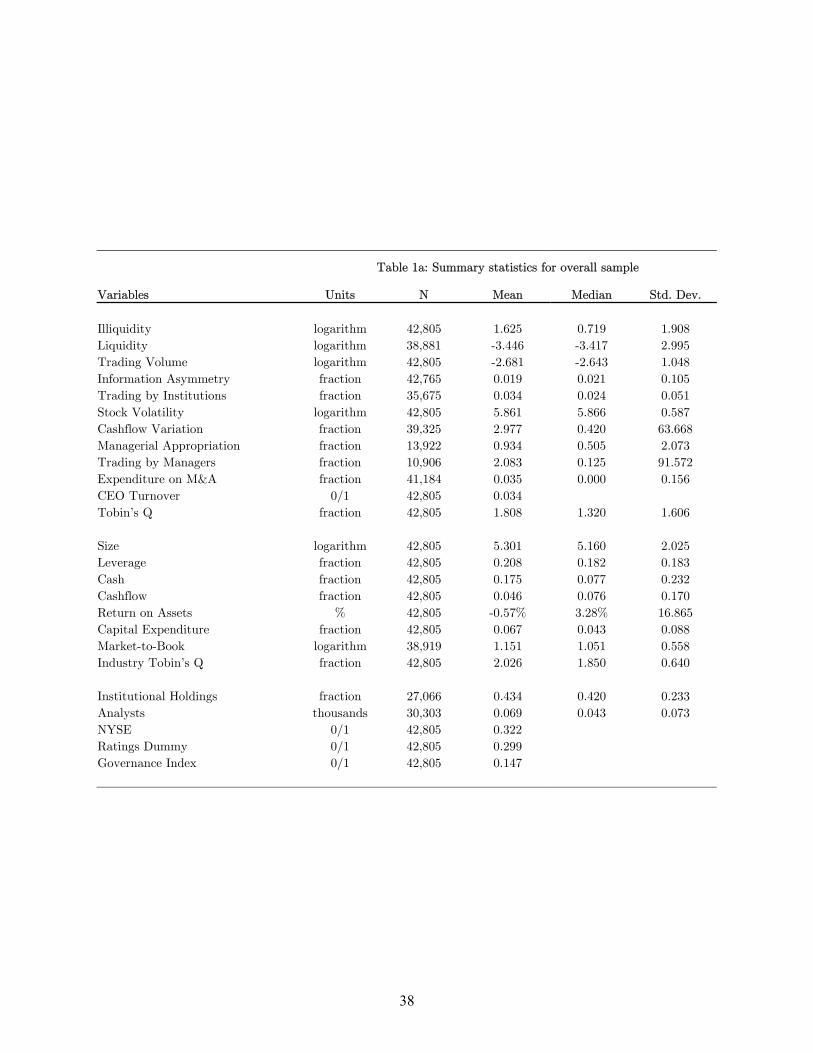
38

Table 1a: Summary statistics for overall sample

Variables Units N Mean Median Std. Dev. Illiquidity logarithm 42,805 1.625 0.719 1.908 Liquidity logarithm 38,881 -3.446 -3.417 2.995 Trading Volume logarithm 42,805 -2.681 -2.643 1.048 Information Asymmetry fraction 42,765 0.019 0.021 0.105 Trading by Institutions fraction 35,675 0.034 0.024 0.051 Stock Volatility logarithm 42,805 5.861 5.866 0.587 Cashflow Variation fraction 39,325 2.977 0.420 63.668 Managerial Appropriation fraction 13,922 0.934 0.505 2.073 Trading by Managers fraction 10,906 2.083 0.125 91.572 Expenditure on M&A fraction 41,184 0.035 0.000 0.156 CEO Turnover 0/1 42,805 0.034 Tobin’s Q fraction 42,805 1.808 1.320 1.606 Size logarithm 42,805 5.301 5.160 2.025 Leverage fraction 42,805 0.208 0.182 0.183 Cash fraction 42,805 0.175 0.077 0.232 Cashflow fraction 42,805 0.046 0.076 0.170 Return on Assets % 42,805 -0.57% 3.28% 16.865 Capital Expenditure fraction 42,805 0.067 0.043 0.088 Market-to-Book logarithm 38,919 1.151 1.051 0.558 Industry Tobin’s Q fraction 42,805 2.026 1.850 0.640 Institutional Holdings fraction 27,066 0.434 0.420 0.233 Analysts thousands 30,303 0.069 0.043 0.073 NYSE 0/1 42,805 0.322 Ratings Dummy 0/1 42,805 0.299 Governance Index 0/1 42,805 0.147

39

Table 1b: Summary statistics for sub-samples

Sub-sample without loans Loan-taking sub-sample Test statistic comparing sub-samples Variables Units N Mean Median Std. Dev. N Mean Median Std. Dev. t-test Wilcoxon rank-test Illiquidity logarithm 25,552 2.035 1.351 2.040 17,253 1.017 0.224 1.502 56.08*** 60.35*** Liquidity logarithm 23,351 -4.148 -4.208 2.914 15,530 -2.392 -2.207 2.799 -59.11*** -56.45*** Trading Volume logarithm 25,552 -2.762 -2.737 1.114 17,253 -2.562 -2.534 0.929 -19.38*** -18.99*** Information Asymmetry fraction 25,521 0.021 0.023 0.098 17,244 0.016 0.018 0.116 4.88*** 4.87*** Trading by Institutions fraction 20,586 0.031 0.021 0.050 15,089 0.037 0.027 0.052 -10.16*** -23.74*** Stock Volatility logarithm 25,552 5.964 5.992 0.609 17,253 5.709 5.699 0.518 45.09*** 46.06*** Cashflow Variation fraction 22,963 3.737 0.483 81.579 16,362 1.912 0.358 20.019 2.80*** 18.85*** Managerial Appropriation fraction 5,754 0.820 0.426 2.166 8,168 1.013 0.557 2.001 -5.42*** -14.40*** Trading by Managers fraction 4,331 1.407 0.131 9.155 6,575 2.529 0.122 117.703 -0.63 0.82 Expenditure on M&A fraction 24,736 0.025 0.000 0.134 16,448 0.051 0.000 0.182 -16.98*** -35.01*** CEO Turnover 0/1 25,552 0.023 - - 17,253 0.051 - - -15.71*** -15.66*** Tobin’s Q fraction 25,552 1.970 1.367 1.886 17,253 1.568 1.269 1.016 25.58*** 15.80*** Size logarithm 25,552 4.672 4.477 1.900 17,253 6.233 6.186 1.837 -84.46*** -80.32*** Leverage fraction 25,552 0.170 0.114 0.178 17,253 0.264 0.260 0.176 -53.79*** -57.23*** Cash fraction 25,552 0.224 0.121 0.260 17,253 0.104 0.042 0.156 54.26*** 54.77*** Cashflow fraction 25,552 0.023 0.068 0.195 17,253 0.080 0.085 0.114 -34.52*** -25.92*** Return on Assets % 25,552 -2.71% 2.74% 19.578 17,253 2.61% 3.83% 11.003 -32.42*** -20.95*** Capital Expenditure fraction 25,552 0.062 0.039 0.081 17,253 0.075 0.048 0.097 -15.03*** -21.90*** Market-to-Book logarithm 22,828 1.172 1.057 0.587 16,091 1.122 1.043 0.513 8.64*** 4.44*** Industry Tobin’s Q fraction 25,552 2.120 2.069 0.655 17,253 1.888 1.667 0.589 37.39*** 36.11*** Institutional Holdings fraction 14,181 0.379 0.339 0.225 12,885 0.494 0.507 0.225 -41.98*** -41.16*** Analysts thousands 16,033 0.058 0.033 0.067 14,270 0.081 0.055 0.077 -27.62*** -33.59*** NYSE 0/1 25,552 0.206 - - 17,253 0.493 - - -65.45*** -62.40*** Ratings Dummy 0/1 25,552 0.172 - - 17,253 0.487 - - -74.16*** -69.81*** Governance Index 0/1 25,552 0.092 - - 17,253 0.229 - - -40.17*** -39.43*** Proximity fraction - - - - 17,253 0.256 0.050 0.346 - - Exclusivity logarithm - - - - 17,014 7.433 7.419 1.395 - - Average Distance thousands km. - - - - 17,220 1.218 0.904 1.042 - - Dispersedness logarithm - - - - 16,994 -3.128 -2.996 1.132 - - *, **, and *** indicate significance at 10%, 5%, and 1% level, respectively.

40

Table 2

Loan-taking decision of the firm and the choice of loan-characteristics In this table, we address the selection bias inherent in our sample of the loan-taking firms as well as the endogeneity of loan-characteristics. It is not by chance that these firms borrow from banks and nor are the characteristics of the loan incidental; rather, it’s an endogenous decision affected by the firm’s characteristics as well as the local bank-lending market.

In Table 2a below, the dependent variable is a dummy variable (LoanDummy) that equals 1 for all the firm-years during which there is an active loan; this variable is zero

otherwise. The firm-years where LoanDummy is equal to one are derived from the Loan Pricing Corporation’s DealScan database and the firm-years where LoanDummy takes the value zero are those firm-years from Compustat for which we had historical firm-location available (see Section 4 for details on our sources of data). Coefficient estimates from a Probit regression for the loan-taking decision are reported in Table 2a. In Table 2b, we present the instruments that we propose as potential determinants of the firms’ loan-characteristics. The dependent variable Proximity is the fraction of the firm’s loan borrowed from banks located within 200 miles (or 320 kilometers) of the firm’s headquarter. Exclusivity is the logarithm of the Herfindahl index of the lending syndicate. The dependent variable Average Distance is the average distance in kilometers between the firm and all the banks in the lending syndicate; the distance is measured between firm’s and banks’ headquarters. Finally, Dispersedness is the logarithm of number of banks in the lending syndicate. OLS estimates for the instrumental variables (besides some other controls) used to instrument for the loan characteristics are reported in Table 2b.

Our independent variables can be grouped into five categories: a) pre-loan characteristics of the local bank-lending market, b) several pre-loan firm-level characteristics, c) lagged banking-market characteristics, d) lagged industry characteristics (of the industry to which the borrowing firm belongs), and e) loan-characteristics of other firms in the industry. All “lagged” variables are recorded at the beginning of the fiscal year while the “pre-loan” variables are measured the year before the loan is initiated.

In order to capture the distinctive features of the local bank-lending market, we employ the following three variables: median size in millions of dollars of all banks (weighted by

the number of branches) available to the borrower in its county of location; median distance in thousands of kilometers (inversely weighted by the number of branches) between the borrower and all local bank-branches’ headquarter location; and concentration of bank-lending market in the county of borrower’s location. We measure this concentration by calculating a Herfindahl Index (ranging between 0—1) of the deposit size across all bank branches in the county; our results are robust if we instead use a Herfindahl Index based simply on the number of branches.

The firm-level control variables that we include in our analysis are the following. First of all, a dummy variable that equals 1 if the firm is located in one of the six largest

metropolises in the US (Boston, Chicago, Los Angeles, New York, Philadelphia, and San Francisco); this is done to account for firms located near large financial markets. Size is measured as the logarithm of book value of assets (item 6). Leverage is the sum of long-term debt (item 9) and debt in current liabilities (item 34), standardized by lagged assets (item 6). Cash is the ratio of total cash (item 1) to lagged assets and Cashflows are defined as income before extraordinary items (item 18) plus depreciation and amortization (item 14), standardized by lagged assets. Capital Expenditure is the ratio of capital expenditures (item 128) to lagged assets. Market-to-Book is the logarithm of the firm’s market-to-book ratio where market-to-book is (item25 x item199)/(item60). Industry Tobin’s Q is the average Q in the industry to which the borrower belongs. Institutional Holdings is the fraction of shares held by those institutional investors that hold at least a 5% position in the firm. Analysts is the number of analysts following the borrowing firm’s stock, and is expressed in thousands for the convenience of obtaining normally-scaled coefficient estimates. NYSE is a dummy variable that takes the value 1 if the firm is listed on the New York Stock Exchange; otherwise the variable is equal to zero. Finally, Ratings Dummy is a dummy variable that equals one if the firm has a credit-rating, and equals zero otherwise.

Industry’s Proximity, Exclusivity, Average Distance, Dispersedness, and Loan-to-Debt Ratio are the averages of those variables for all the loan-taking firms in the corresponding

industry except the specific borrowing firm itself. Proximity, Exclusivity, Average Distance, and Dispersedness are as described above, and Loan-to-Debt Ratio is the ratio of loan amount to lagged long-term debt (item 9) used as a control variable. Industry’s size, leverage, cash, cashflow, capital expenditure, and market-to-book is average of these variables (as defined above) for all other firms in the corresponding industry except the borrowing firm itself.

Of course, besides all the variables described above, there might be some macroeconomic or regulatory variables that can also influence the firm’s loan-taking decision. We hope

to capture those using year effects through the Time Dummies used in our regressions. We use the estimates of column (2) of Table 2a below to calculate the Lambda (Inverse Mills’ Ratio) used in subsequent analyses. Industries are categorized by 1-digit SIC

Code. All z-statistics in Table 2a and t-statistics in Table 2b are calculated using robust standard errors clustered by firm.

41

Table 2a: Loan-taking Decision

Independent variables: (1) (2)

Median Size of Banks 0.262

[0.22]

Median Distance from Banks -0.353**

[2.52]

Lending market Concentration 0.310

[1.41]

Metropolis -0.098*

[1.65]

Size 0.081*** 0.112***

[4.63] [5.90]

Leverage 1.320*** 1.320***

[12.96] [12.87]

Cash -0.610*** -0.611***

[6.26] [6.09]

Cashflows 0.571*** 0.658***

[4.56] [4.98]

Capital Expenditure 0.494*** 0.398**

[2.74] [2.16]

Market-to-Book -0.051* -0.044

[1.76] [1.48]

Institutional Holdings 0.773*** 0.470***

[9.44] [5.50]

Analysts -1.152*** -1.211***

[3.79] [3.87]

NYSE 0.108** 0.119***

[2.56] [2.77]

Ratings Dummy 0.267*** 0.330***

[5.99] [7.32]

Constant -1.080*** -1.775***

[12.46] [5.99]

Observations 23085 23084

Pseudo R-squared 0.14 0.17

Time Dummies No Yes

Industry Dummies No Yes

Robust z statistics in brackets

* significant at 10%; ** significant at 5%; *** significant at 1%

42

Table 2b: Instruments for loan characteristics

Proximity Exclusivity

Average Distance Dispersedness

Independent variables: Pre-loan Median Size of Banks -1.290** 0.069 8.505*** -0.408 [2.24] [0.04] [4.34] [0.29] Pre-loan Median Distance from Banks -0.194** 0.702*** 2.177*** -0.646*** [2.38] [3.08] [7.07] [3.67] Pre-loan Lending market Concentration -0.032 0.271 -0.545** -0.197 [0.33] [0.80] [2.05] [0.80] Metropolis 0.114*** 0.06 -0.176** -0.082* [5.69] [0.97] [2.41] [1.78] Pre-loan Leverage -0.065* -1.478*** 0.003 1.043*** [1.80] [11.93] [0.03] [11.36] Pre-loan Size -0.035*** -0.462*** 0.086*** 0.436*** [9.40] [40.06] [7.82] [55.30] Pre-loan Cash 0.038** 0.110** -0.001 -0.067 [2.31] [2.09] [0.02] [1.28] Pre-loan Cashflows -0.029 -0.463*** 0.112 0.451*** [0.66] [3.90] [0.71] [4.65] Pre-loan Capital Expenditure -0.117*** -0.299** 0.254* 0.028 [2.84] [1.97] [1.72] [0.24] Pre-loan Market-to-Book 0.460*** -0.523** -0.862* 0.491** [4.17] [2.02] [1.82] [2.09] Lagged Median Size of Banks -0.100 0.446 7.619*** -0.663 [0.18] [0.24] [4.03] [0.48] Lagged Median Distance from Banks 0.000 0.000*** 0.001*** -0.000** [0.67] [3.27] [6.43] [2.40] Lagged Lending market Concentration 0.11 -0.149 -1.079*** 0.074 [1.18] [0.43] [4.19] [0.29] Lagged Industry Size 0.01 0.116*** -0.034 -0.090*** [0.91] [3.06] [0.90] [3.03] Lagged Industry Leverage -0.052 -0.262 0.612** -0.086 [0.66] [0.81] [2.10] [0.37] Lagged Industry Cash 0.126** 0.052 0.266 -0.196 [2.53] [0.32] [1.60] [1.58] Lagged Industry Cashflows -0.066 -0.365 0.462* 0.287 [0.85] [1.47] [1.73] [1.47] Lagged Industry Capital Expenditure -0.183* -0.142 0.236 0.257 [1.86] [0.40] [0.63] [0.94] Lagged Industry Market-to-Book -0.001 -0.006*** 0.000 0.005*** [1.37] [2.68] [0.20] [3.35] Lagged Industry's Proximity 0.074 0.139 [1.05] [0.62] Lagged Industry's Exclusivity 0.002 0.081 [0.15] [1.48] Lagged Industry's Avg. Distance 0.146** -0.049 [2.17] [0.94] Lagged Industry's Dispersedness -0.051 0.037 [0.79] [0.66] Lagged Industry's Loan-to-Debt Ratio 0.000** 0.000 -0.000* 0.000 [2.14] [0.51] [1.90] [1.07] Constant 0.289* 9.882*** 0.221 -5.631*** [1.82] [18.05] [0.56] [13.94] Observations 11712 11530 11700 11518 (pseudo/adj) R-square 0.09 0.44 0.16 0.55 Time Dummies Yes Yes Yes Yes Industry Dummies Yes Yes Yes Yes Robust t statistics are in brackets * significant at 10%; ** significant at 5%; *** significant at 1%

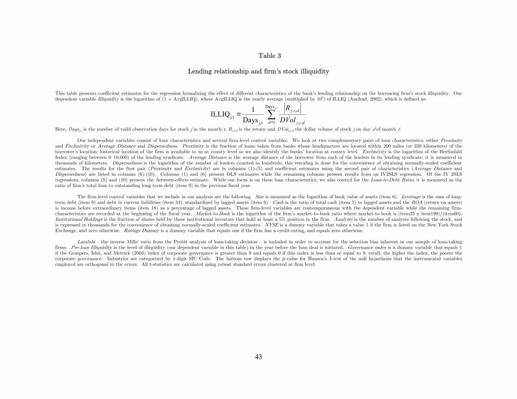
43

Table 3

Lending relationship and firm’s stock illiquidity This table presents coefficient estimates for the regression formalizing the effect of different characteristics of the bank’s lending relationship on the borrowing firm’s stock illiquidity. Our dependent variable Illiquidity is the logarithm of (1 + AvgILLIQ), where AvgILLIQ is the yearly average (multiplied by 107) of ILLIQ (Amihud, 2002), which is defined as:

∑=

=tj,Days

1 ,,

,,

tj,tj, Days

1 ILLIQd dtj

dtj

DVol

R

Here, Daysj,t is the number of valid observation days for stock j in the month t, Rj,t,d is the return and DVolj,t,d the dollar volume of stock j on day d of month t.

Our independent variables consist of loan characteristics and several firm-level control variables. We look at two complementary pairs of loan characteristics: either Proximity and Exclusivity or Average Distance and Dispersedness. Proximity is the fraction of loans taken from banks whose headquarters are located within 200 miles (or 320 kilometers) of the borrower’s location; historical location of the firm is available to us at county level so we also identify the banks’ location at county level. Exclusivity is the logarithm of the Herfindahl Index (ranging between 0—10,000) of the lending syndicate. Average Distance is the average distance of the borrower from each of the lenders in its lending syndicate; it is measured in thousands of kilometers. Dispersedness is the logarithm of the number of lenders counted in hundreds; this rescaling is done for the convenience of obtaining normally-scaled coefficient estimates. The results for the first pair (Proximity and Exclusivity) are in columns (1)-(5) and coefficient estimates using the second pair of characteristics (Average Distance and Dispersedness) are listed in columns (6)-(10). Columns (1) and (6) present OLS estimates while the remaining columns present results from an IV2SLS regression. Of the IV 2SLS regressions, columns (5) and (10) present the between-effects estimate. While our focus is on these loan characteristics, we also control for the Loan-to-Debt Ratio; it is measured as the ratio of firm’s total loan to outstanding long-term debt (item 9) in the previous fiscal year.

The firm-level control variables that we include in our analysis are the following. Size is measured as the logarithm of book value of assets (item 6). Leverage is the sum of long-

term debt (item 9) and debt in current liabilities (item 34), standardized by lagged assets (item 6). Cash is the ratio of total cash (item 1) to lagged assets and the ROA (return on assets) is income before extraordinary items (item 18) as a percentage of lagged assets. These firm-level variables are contemporaneous with the dependent variable while the remaining firm-characteristics are recorded at the beginning of the fiscal year. Market-to-Book is the logarithm of the firm’s market-to-book ratio where market-to-book is (item25 x item199)/(item60). Institutional Holdings is the fraction of shares held by those institutional investors that hold at least a 5% position in the firm. Analysts is the number of analysts following the stock, and is expressed in thousands for the convenience of obtaining normally-scaled coefficient estimates. NYSE is a dummy variable that takes a value 1 if the firm is listed on the New York Stock Exchange, and zero otherwise. Ratings Dummy is a dummy variable that equals one if the firm has a credit-rating, and equals zero otherwise.

Lambda — the inverse Mills’ ratio from the Probit analysis of loan-taking decision — is included in order to account for the selection bias inherent in our sample of loan-taking

firms. Pre-loan Illiquidity is the level of illiquidity (our dependent variable in this table) in the year before the loan deal is initiated. Governance index is a dummy variable that equals 1 if the Gompers, Ishii, and Metrick (2003) index of corporate governance is greater than 9 and equals 0 if this index is less than or equal to 9; recall, the higher the index, the poorer the corporate governance. Industries are categorized by 1-digit SIC Code. The bottom row displays the p-value for Hansen’s J-test of the null hypothesis that the instrumental variables employed are orthogonal to the errors. All t-statistics are calculated using robust standard errors clustered at firm level.

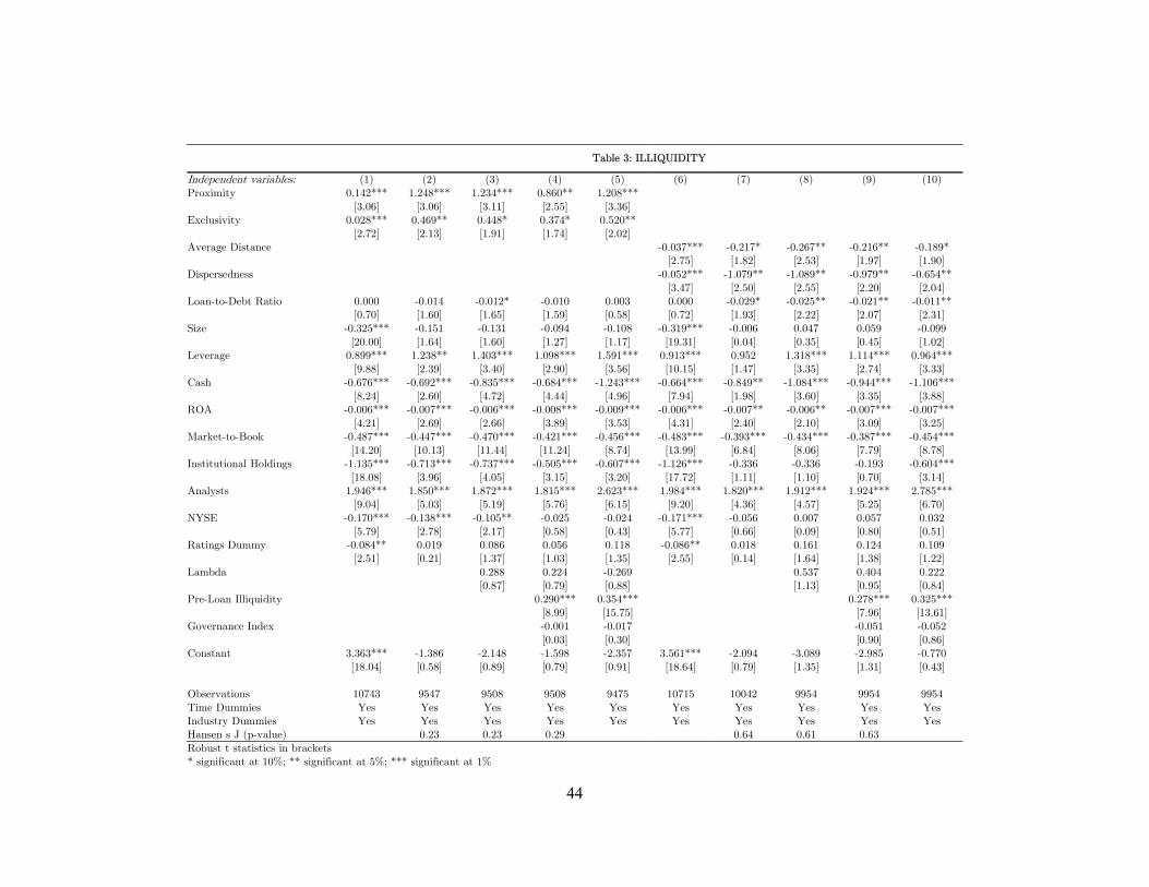
44

Table 3: ILLIQUIDITY

Independent variables: (1) (2) (3) (4) (5) (6) (7) (8) (9) (10) Proximity 0.142*** 1.248*** 1.234*** 0.860** 1.208*** [3.06] [3.06] [3.11] [2.55] [3.36] Exclusivity 0.028*** 0.469** 0.448* 0.374* 0.520** [2.72] [2.13] [1.91] [1.74] [2.02] Average Distance -0.037*** -0.217* -0.267** -0.216** -0.189* [2.75] [1.82] [2.53] [1.97] [1.90] Dispersedness -0.052*** -1.079** -1.089** -0.979** -0.654** [3.47] [2.50] [2.55] [2.20] [2.04] Loan-to-Debt Ratio 0.000 -0.014 -0.012* -0.010 0.003 0.000 -0.029* -0.025** -0.021** -0.011** [0.70] [1.60] [1.65] [1.59] [0.58] [0.72] [1.93] [2.22] [2.07] [2.31] Size -0.325*** -0.151 -0.131 -0.094 -0.108 -0.319*** -0.006 0.047 0.059 -0.099 [20.00] [1.64] [1.60] [1.27] [1.17] [19.31] [0.04] [0.35] [0.45] [1.02] Leverage 0.899*** 1.238** 1.403*** 1.098*** 1.591*** 0.913*** 0.952 1.318*** 1.114*** 0.964*** [9.88] [2.39] [3.40] [2.90] [3.56] [10.15] [1.47] [3.35] [2.74] [3.33] Cash -0.676*** -0.692*** -0.835*** -0.684*** -1.243*** -0.664*** -0.849** -1.084*** -0.944*** -1.106*** [8.24] [2.60] [4.72] [4.44] [4.96] [7.94] [1.98] [3.60] [3.35] [3.88] ROA -0.006*** -0.007*** -0.006*** -0.008*** -0.009*** -0.006*** -0.007** -0.006** -0.007*** -0.007*** [4.21] [2.69] [2.66] [3.89] [3.53] [4.31] [2.40] [2.10] [3.09] [3.25] Market-to-Book -0.487*** -0.447*** -0.470*** -0.421*** -0.456*** -0.483*** -0.393*** -0.434*** -0.387*** -0.454*** [14.20] [10.13] [11.44] [11.24] [8.74] [13.99] [6.84] [8.06] [7.79] [8.78] Institutional Holdings -1.135*** -0.713*** -0.737*** -0.505*** -0.607*** -1.126*** -0.336 -0.336 -0.193 -0.604*** [18.08] [3.96] [4.05] [3.15] [3.20] [17.72] [1.11] [1.10] [0.70] [3.14] Analysts 1.946*** 1.850*** 1.872*** 1.815*** 2.623*** 1.984*** 1.820*** 1.912*** 1.924*** 2.785*** [9.04] [5.03] [5.19] [5.76] [6.15] [9.20] [4.36] [4.57] [5.25] [6.70] NYSE -0.170*** -0.138*** -0.105** -0.025 -0.024 -0.171*** -0.056 0.007 0.057 0.032 [5.79] [2.78] [2.17] [0.58] [0.43] [5.77] [0.66] [0.09] [0.80] [0.51] Ratings Dummy -0.084** 0.019 0.086 0.056 0.118 -0.086** 0.018 0.161 0.124 0.109 [2.51] [0.21] [1.37] [1.03] [1.35] [2.55] [0.14] [1.64] [1.38] [1.22] Lambda 0.288 0.224 -0.269 0.537 0.404 0.222 [0.87] [0.79] [0.88] [1.13] [0.95] [0.84] Pre-Loan Illiquidity 0.290*** 0.354*** 0.278*** 0.325*** [8.99] [15.75] [7.96] [13.61] Governance Index -0.001 -0.017 -0.051 -0.052 [0.03] [0.30] [0.90] [0.86] Constant 3.363*** -1.386 -2.148 -1.598 -2.357 3.561*** -2.094 -3.089 -2.985 -0.770 [18.04] [0.58] [0.89] [0.79] [0.91] [18.64] [0.79] [1.35] [1.31] [0.43] Observations 10743 9547 9508 9508 9475 10715 10042 9954 9954 9954 Time Dummies Yes Yes Yes Yes Yes Yes Yes Yes Yes Yes Industry Dummies Yes Yes Yes Yes Yes Yes Yes Yes Yes Yes Hansen's J (p-value) 0.23 0.23 0.29 0.64 0.61 0.63 Robust t statistics in brackets * significant at 10%; ** significant at 5%; *** significant at 1%

45

Table 4

Lending relationship and firm’s stock liquidity

This table presents results that serve as a robustness check for those presented in Table 3 (for stock’s illiquidity) above; here, we formalize the effect of different characteristics of the lending relationship on the firm’s stock liquidity (instead of illiquidity). Our dependent variable Liquidity is the logarithm of “Amivest” liquidity ratio, which is obtained from Prof. Joel Hasbrouck’s webpage: http://pages.stern.nyu.edu/~jhasbrou/Research/GibbsEstimates/Liquidity%20estimates.htm. In fact, it is simply the reciprocal of the illiquidity ratio defined in Table 3 above.

Our independent variables consist of loan characteristics and several firm-level control variables. We look at two complementary pairs of loan characteristics: either Proximity and Exclusivity or Average Distance and Dispersedness. Proximity is the fraction of loans taken from banks whose headquarters are located within 200 miles (or 320 kilometers) of the borrower’s location; historical location of the firm is available to us at county level so we also identify the banks’ location at county level. Exclusivity is the logarithm of the Herfindahl Index (ranging between 0—10,000) of the lending syndicate. Average Distance is the average distance of the borrower from each of the lenders in its lending syndicate; it is measured in thousands of kilometers. Dispersedness is the logarithm of the number of lenders counted in hundreds; this rescaling is done for the convenience of obtaining normally-scaled coefficient estimates. The results for the first pair (Proximity and Exclusivity) are in columns (1)-(5) and coefficient estimates using the second pair of characteristics (Average Distance and Dispersedness) are listed in columns (6)-(10). Columns (1) and (6) present OLS estimates while the remaining columns present results from an IV2SLS regression. Of the IV 2SLS regressions, columns (5) and (10) present the between-effects estimate. While our focus is on these loan characteristics, we also control for the Loan-to-Debt Ratio; it is measured as the ratio of firm’s total loan to outstanding long-term debt (item 9) in the previous fiscal year.

The firm-level control variables that we include in our analysis are the following. Size is measured as the logarithm of book value of assets (item 6). Leverage is the sum of long-

term debt (item 9) and debt in current liabilities (item 34), standardized by lagged assets (item 6). Cash is the ratio of total cash (item 1) to lagged assets and the ROA (return on assets) is income before extraordinary items (item 18) as a percentage of lagged assets. These firm-level variables are contemporaneous with the dependent variable while the remaining firm-characteristics are recorded at the beginning of the fiscal year. Market-to-Book is the logarithm of the firm’s market-to-book ratio where market-to-book is (item25 x item199)/(item60). Institutional Holdings is the fraction of shares held by those institutional investors that hold at least a 5% position in the firm. Analysts is the number of analysts following the stock, and is expressed in thousands for the convenience of obtaining normally-scaled coefficient estimates. NYSE is a dummy variable that takes a value 1 if the firm is listed on the New York Stock Exchange, and zero otherwise. Ratings Dummy is a dummy variable that equals one if the firm has a credit-rating, and equals zero otherwise.

Lambda — the inverse Mills’ ratio from the Probit analysis of loan-taking decision — is included in order to account for the selection bias inherent in our sample of loan-taking

firms. Pre-loan Liquidity is the level of liquidity (our dependent variable in this table) in the year before the loan deal is initiated. Governance index is a dummy variable that equals 1 if the Gompers, Ishii, and Metrick (2003) index of corporate governance is greater than 9 and equals 0 if this index is less than or equal to 9; recall, the higher the index, the poorer the corporate governance. Industries are categorized by 1-digit SIC Code. The bottom row displays the p-value for Hansen’s J-test of the null hypothesis that the instrumental variables employed are orthogonal to the errors. All t-statistics are calculated using robust standard errors clustered at firm level.

46

Table 4: LIQUIDITY

Independent variables: (1) (2) (3) (4) (5) (6) (7) (8) (9) (10) Proximity -0.060 -1.392** -1.364** -1.186** -1.163** [1.21] [2.31] [2.33] [2.14] [2.45] Exclusivity -0.005 -1.040*** -0.746** -0.861** -0.860** [0.44] [2.76] [2.10] [2.54] [2.20] Average Distance 0.051*** 0.519* 0.543* 0.502** 0.560** [3.10] [1.67] [1.96] [2.04] [2.20] Dispersedness 0.006 2.120** 1.853** 1.523** 1.508** [0.30] [2.42] [2.16] [2.17] [2.27] Loan-to-Debt Ratio 0.000 0.056*** 0.060*** 0.053*** 0.029*** 0.000 0.063* 0.070** 0.061** 0.026*** [0.09] [2.81] [2.98] [2.88] [3.58] [0.09] [1.74] [2.40] [2.42] [2.93] Size 0.986*** 0.672*** 0.688*** 0.494*** 0.536*** 0.987*** 0.387 0.379 0.313 0.367* [46.77] [5.02] [5.31] [3.56] [3.46] [46.17] [1.24] [1.43] [1.31] [1.66] Leverage -2.143*** -2.467*** -2.402*** -2.320*** -2.035*** -2.173*** -2.490* -2.655*** -2.165*** -2.208*** [18.57] [3.75] [3.71] [3.86] [3.13] [18.87] [1.78] [2.97] [2.86] [3.31] Cash 1.243*** 0.816* 1.030*** 1.059*** 1.425*** 1.206*** 1.262 1.392** 1.232** 1.708*** [9.49] [1.80] [2.58] [2.91] [3.47] [9.27] [1.45] [2.24] [2.35] [3.22] ROA 0.015*** 0.024*** 0.022*** 0.023*** 0.025*** 0.015*** 0.024*** 0.022*** 0.024*** 0.024*** [8.33] [4.25] [3.97] [4.71] [5.91] [8.36] [3.30] [3.39] [4.26] [5.43] Market-to-Book 1.287*** 1.185*** 1.259*** 1.169*** 1.046*** 1.286*** 1.086*** 1.164*** 1.091*** 0.972*** [20.51] [11.57] [13.24] [12.69] [11.02] [20.61] [8.06] [8.94] [9.07] [8.35] Institutional Holdings 1.841*** 0.802** 0.962*** 0.609* 0.634* 1.853*** 0.207 0.315 0.277 0.451 [21.22] [2.01] [2.64] [1.66] [1.76] [21.28] [0.31] [0.48] [0.49] [0.96] Analysts 2.769*** 3.019*** 2.750*** 1.770*** 2.039*** 2.676*** 2.386*** 2.241** 0.979 1.115 [8.35] [4.16] [3.98] [2.76] [2.73] [8.07] [2.68] [2.56] [1.30] [1.28] NYSE -0.329*** -0.371*** -0.482*** -0.520*** -0.476*** -0.325*** -0.526*** -0.634*** -0.622*** -0.592*** [8.23] [3.53] [4.00] [4.50] [4.71] [8.13] [3.05] [3.51] [3.98] [4.65] Ratings Dummy 0.172*** 0.072 -0.111 -0.128 -0.004 0.167*** -0.089 -0.298 -0.266 -0.155 [3.88] [0.51] [0.70] [0.87] [0.02] [3.78] [0.32] [1.35] [1.38] [0.83] Lambda -1.291 -1.068 -0.079 -1.356 -1.300 -0.200 [1.63] [1.55] [0.16] [1.21] [1.35] [0.39] Pre-Loan Liquidity 0.186*** 0.193*** 0.211*** 0.200*** [5.57] [6.14] [4.30] [5.53] Governance Index 0.165* 0.306*** 0.231** 0.336*** [1.85] [2.73] [2.12] [2.78] Constant -10.586*** 0.575 -1.363 1.186 1.051 -10.725*** 0.104 1.078 0.903 -0.866 [19.23] [0.14] [0.37] [0.32] [0.25] [20.58] [0.02] [0.23] [0.22] [0.23] Observations 9536 8421 8384 8384 8481 9513 8411 8372 8372 8372 Time Dummies Yes Yes Yes Yes Yes Yes Yes Yes Yes Yes Industry Dummies Yes Yes Yes Yes Yes Yes Yes Yes Yes Yes Hansen's J (p-value) 0.29 0.34 0.47 0.30 0.48 0.27 Robust t statistics in brackets * significant at 10%; ** significant at 5%; *** significant at 1%

47

Table 5

Lending relationship and trading volume This table presents coefficient estimates for the regression depicting the effect of the characteristics of bank’s lending relationship on the borrowing firm’s stock trading volume. If volume is defined as the number of shares traded as a fraction of total shares outstanding, then our dependent variable, Trading Volume, is the logarithm of average monthly volume over the year.

Our independent variables consist of loan characteristics and several firm-level control variables. We look at two complementary pairs of loan characteristics: either Proximity and Exclusivity or Average Distance and Dispersedness. Proximity is the fraction of loans taken from banks whose headquarters are located within 200 miles (or 320 kilometers) of the borrower’s location; historical location of the firm is available to us at county level so we also identify the banks’ location at county level. Exclusivity is the logarithm of the Herfindahl Index (ranging between 0—10,000) of the lending syndicate. Average Distance is the average distance of the borrower from each of the lenders in its lending syndicate; it is measured in thousands of kilometers. Dispersedness is the logarithm of the number of lenders counted in hundreds; this rescaling is done for the convenience of obtaining normally-scaled coefficient estimates. The results for the first pair (Proximity and Exclusivity) are in columns (1)-(5) and coefficient estimates using the second pair of characteristics (Average Distance and Dispersedness) are listed in columns (6)-(10). Columns (1) and (6) present OLS estimates while the remaining columns present results from an IV2SLS regression. Of the IV 2SLS regressions, columns (5) and (10) present the between-effects estimate. While our focus is on these loan characteristics, we also control for the Loan-to-Debt Ratio; it is measured as the ratio of firm’s total loan to outstanding long-term debt (item 9) in the previous fiscal year.

The firm-level control variables that we include in our analysis are the following. Size is measured as the logarithm of book value of assets (item 6). Leverage is the sum of long-

term debt (item 9) and debt in current liabilities (item 34), standardized by lagged assets (item 6). Cash is the ratio of total cash (item 1) to lagged assets and the ROA (return on assets) is income before extraordinary items (item 18) as a percentage of lagged assets. These firm-level variables are contemporaneous with the dependent variable while the remaining firm-characteristics are recorded at the beginning of the fiscal year. Market-to-Book is the logarithm of the firm’s market-to-book ratio where market-to-book is (item25 x item199)/(item60). Institutional Holdings is the fraction of shares held by those institutional investors that hold at least a 5% position in the firm. Analysts is the number of analysts following the stock, and is expressed in thousands for the convenience of obtaining normally-scaled coefficient estimates. NYSE is a dummy variable that takes a value 1 if the firm is listed on the New York Stock Exchange, and zero otherwise. Ratings Dummy is a dummy variable that equals one if the firm has a credit-rating, and equals zero otherwise.

Lambda — the inverse Mills’ ratio from the Probit analysis of loan-taking decision — is included in order to account for the selection bias inherent in our sample of loan-taking

firms. Pre-loan Volume is the level of trading volume (our dependent variable in this table) in the year before the loan deal is initiated. Governance index is a dummy variable that equals 1 if the Gompers, Ishii, and Metrick (2003) index of corporate governance is greater than 9 and equals 0 if this index is less than or equal to 9; recall, the higher the index, the poorer the corporate governance. Industries are categorized by 1-digit SIC Code. The bottom row displays the p-value for Hansen’s J-test of the null hypothesis that the instrumental variables employed are orthogonal to the errors. All t-statistics are calculated using robust standard errors clustered at firm level.

48

Table 5: TRADING VOLUME

Independent variables: (1) (2) (3) (4) (5) (6) (7) (8) (9) (10) Proximity -0.136*** -1.355*** -1.368*** -0.988*** -0.697*** [3.73] [5.01] [4.88] [3.84] [3.27] Exclusivity -0.026*** -0.515*** -0.548*** -0.519*** -0.440*** [2.81] [3.24] [3.40] [3.55] [2.94] Average Distance 0.065*** 0.162*** 0.165*** 0.109*** 0.095*** [5.25] [4.01] [3.99] [2.87] [2.64] Dispersedness 0.014 0.695*** 0.663*** 0.617*** 0.651*** [1.01] [3.22] [3.31] [3.48] [3.12] Loan-to-Debt Ratio 0.001** 0.015** 0.016** 0.013** 0.005* 0.001*** 0.020** 0.023*** 0.017** 0.006* [2.53] [2.06] [2.23] [2.05] [1.68] [2.89] [2.16] [2.61] [2.39] [1.80] Size 0.015 -0.161*** -0.160** -0.130** -0.108* 0.022 -0.174*** -0.174*** -0.133** -0.160** [1.12] [2.68] [2.57] [2.33] [1.93] [1.60] [2.64] [2.67] [2.39] [2.44] Leverage -0.231*** -0.759*** -0.725*** -0.669*** -0.488* -0.204*** -0.310 -0.294 -0.291* -0.425* [2.99] [2.88] [2.69] [2.75] [1.82] [2.67] [1.48] [1.53] [1.68] [1.83] Cash 1.426*** 1.510*** 1.459*** 1.151*** 1.290*** 1.373*** 1.494*** 1.494*** 1.224*** 1.470*** [17.65] [8.00] [8.17] [7.42] [7.44] [17.11] [7.61] [7.60] [7.42] [6.88] ROA -0.007*** -0.006*** -0.005** -0.002 -0.001 -0.007*** -0.006*** -0.006*** -0.003 -0.004* [6.47] [2.73] [2.49] [1.27] [0.77] [6.24] [2.61] [2.64] [1.55] [1.95] Market-to-Book 0.213*** 0.178*** 0.169*** 0.162*** 0.152*** 0.208*** 0.138*** 0.148*** 0.141*** 0.138*** [8.34] [4.60] [4.40] [4.80] [3.83] [8.19] [3.27] [3.70] [4.11] [3.24] Institutional Holdings 1.306*** 0.875*** 0.843*** 0.570*** 0.710*** 1.326*** 0.801*** 0.802*** 0.561*** 0.671*** [20.02] [5.11] [4.97] [3.83] [5.51] [20.35] [4.03] [4.40] [3.74] [4.70] Analysts 1.047*** 1.049*** 1.037*** 0.454 0.685** 0.963*** 0.967*** 0.925*** 0.315 0.620* [4.81] [3.04] [2.91] [1.45] [2.11] [4.46] [3.00] [2.85] [1.15] [1.95] NYSE -0.487*** -0.513*** -0.506*** -0.365*** -0.355*** -0.484*** -0.532*** -0.550*** -0.397*** -0.404*** [16.81] [10.64] [9.19] [6.93] [7.79] [16.73] [9.91] [9.05] [7.12] [7.94] Ratings Dummy 0.185*** 0.078 0.104 0.057 0.028 0.182*** 0.127** 0.101 0.060 -0.003 [5.77] [1.27] [1.63] [1.02] [0.43] [5.72] [2.05] [1.42] [1.01] [0.04] Lambda 0.117 0.059 0.163 -0.209 -0.160 -0.049 [0.46] [0.27] [0.76] [0.67] [0.64] [0.24] Pre-Loan Volume 0.369*** 0.405*** 0.369*** 0.395*** [12.39] [16.06] [12.50] [15.22] Governance Index 0.064 0.078* 0.069* 0.081* [1.59] [1.79] [1.86] [1.82] Constant -3.480*** 1.779 2.412 2.548* 2.318 -3.900*** -0.043 0.057 0.861 1.238 [13.91] [1.10] [1.34] [1.72] [1.45] [18.28] [0.04] [0.05] [0.84] [1.07] Observations 10743 9547 9508 9508 9508 10715 9532 9492 9492 9492 Time Dummies Yes Yes Yes Yes Yes Yes Yes Yes Yes Yes Industry Dummies Yes Yes Yes Yes Yes Yes Yes Yes Yes Yes Hansen's J (p-value) 0.48 0.57 0.92 0.26 0.32 0.70 Robust t statistics in brackets * significant at 10%; ** significant at 5%; *** significant at 1%

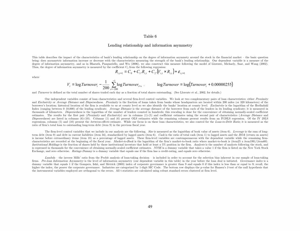
49

Table 6

Lending relationship and information asymmetry

This table describes the impact of the characteristics of bank’s lending relationship on the degree of information asymmety around the stock in the financial market — the basic question being: does asymmetric information increase or decrease with the characteristics measuring the strength of the bank’s lending relationship. Our dependent variable is a measure of the degree of information asymmetry, and as in Bharath, Pasquariello, and Wu (2006), we also construct this measure following the model of Llorente, Michaely, Saar, and Wang (2002). Thus, the degree of information asymmetry is measured by the coefficient C2 from the following regression:

( ) 1,,,2,101, .. ++ +×++= tititititi RVCRCCR ε

where

∑−

−=+−=

1

200log

2001log

ssttt TurnoverTurnoverV , ( )00000255.0loglog += tTurnoverTurnover

and Turnover is defined as the total number of shares traded each day as a fraction of total shares outstanding. (See Llorente et al., 2002, for details.)

Our independent variables consist of loan characteristics and several firm-level control variables. We look at two complementary pairs of loan characteristics: either Proximity and Exclusivity or Average Distance and Dispersedness. Proximity is the fraction of loans taken from banks whose headquarters are located within 200 miles (or 320 kilometers) of the borrower’s location; historical location of the firm is available to us at county level so we also identify the banks’ location at county level. Exclusivity is the logarithm of the Herfindahl Index (ranging between 0—10,000) of the lending syndicate. Average Distance is the average distance of the borrower from each of the lenders in its lending syndicate; it is measured in thousands of kilometers. Dispersedness is the logarithm of the number of lenders counted in hundreds; this rescaling is done for the convenience of obtaining normally-scaled coefficient estimates. The results for the first pair (Proximity and Exclusivity) are in columns (1)-(5) and coefficient estimates using the second pair of characteristics (Average Distance and Dispersedness) are listed in columns (6)-(10). Columns (1) and (6) present OLS estimates while the remaining columns present results from an IV2SLS regression. Of the IV 2SLS regressions, columns (5) and (10) present the between-effects estimate. While our focus is on these loan characteristics, we also control for the Loan-to-Debt Ratio; it is measured as the ratio of firm’s total loan to outstanding long-term debt (item 9) in the previous fiscal year.

The firm-level control variables that we include in our analysis are the following. Size is measured as the logarithm of book value of assets (item 6). Leverage is the sum of long-

term debt (item 9) and debt in current liabilities (item 34), standardized by lagged assets (item 6). Cash is the ratio of total cash (item 1) to lagged assets and the ROA (return on assets) is income before extraordinary items (item 18) as a percentage of lagged assets. These firm-level variables are contemporaneous with the dependent variable while the remaining firm-characteristics are recorded at the beginning of the fiscal year. Market-to-Book is the logarithm of the firm’s market-to-book ratio where market-to-book is (item25 x item199)/(item60). Institutional Holdings is the fraction of shares held by those institutional investors that hold at least a 5% position in the firm. Analysts is the number of analysts following the stock, and is expressed in thousands for the convenience of obtaining normally-scaled coefficient estimates. NYSE is a dummy variable that takes a value 1 if the firm is listed on the New York Stock Exchange, and zero otherwise. Ratings Dummy is a dummy variable that equals one if the firm has a credit-rating, and equals zero otherwise.

Lambda — the inverse Mills’ ratio from the Probit analysis of loan-taking decision — is included in order to account for the selection bias inherent in our sample of loan-taking

firms. Pre-loan Information Asymmetry is the level of information asymmetry (our dependent variable in this table) in the year before the loan deal is initiated. Governance index is a dummy variable that equals 1 if the Gompers, Ishii, and Metrick (2003) index of corporate governance is greater than 9 and equals 0 if this index is less than or equal to 9; recall, the higher the index, the poorer the corporate governance. Industries are categorized by 1-digit SIC Code. The bottom row displays the p-value for Hansen’s J-test of the null hypothesis that the instrumental variables employed are orthogonal to the errors. All t-statistics are calculated using robust standard errors clustered at firm level.

50

Table 6: INFORMATION ASYMMETRY

Independent variables: (1) (2) (3) (4) (5) (6) (7) (8) (9) (10) Proximity 0.007** 0.101*** 0.103*** 0.105*** 0.061* [2.00] [2.75] [2.71] [2.65] [1.81] Exclusivity 0.002** 0.059** 0.062** 0.064* 0.052* [2.04] [2.17] [1.96] [1.93] [1.77] Average Distance -0.004*** -0.013** -0.011** -0.010** -0.010* [3.25] [2.08] [2.01] [1.96] [1.92] Dispersedness -0.004** -0.133** -0.111** -0.106** -0.069** [2.55] [2.44] [2.21] [2.14] [2.04] Loan-to-Debt Ratio 0.000 0.000 0.000 0.000 0.001 0.000 0.000 -0.001 -0.001 0.000 [0.51] [0.32] [0.14] [0.20] [1.61] [0.40] [0.15] [0.90] [0.87] [0.51] Size 0.001 0.024** 0.023** 0.023* 0.019* 0.001 0.044** 0.035** 0.032** 0.022** [0.44] [2.23] [2.04] [1.94] [1.77] [0.63] [2.34] [2.30] [2.20] [2.08] Leverage 0.010 0.125** 0.114** 0.118** 0.098** 0.010 0.129* 0.089** 0.090** 0.073** [1.15] [2.44] [2.24] [2.26] [2.18] [1.18] [1.91] [2.18] [2.21] [2.14] Cash -0.035*** -0.075*** -0.064*** -0.065*** -0.079*** -0.033*** -0.119** -0.090*** -0.088*** -0.087*** [3.91] [3.38] [3.66] [3.59] [2.99] [3.61] [2.55] [3.12] [3.11] [2.76] ROA 0.000 0.000 0.000 0.000 0.000 -0.000* 0.000 0.000 0.000 0.000 [1.54] [0.70] [1.28] [1.15] [0.72] [1.67] [0.14] [0.90] [0.73] [0.15] Market-to-Book -0.009*** -0.007* -0.005 -0.006 0.000 -0.009*** -0.002 -0.001 -0.002 0.000 [3.13] [1.77] [1.25] [1.30] [0.04] [3.02] [0.46] [0.23] [0.40] [0.08] Institutional Holdings -0.024*** 0.017 0.021 0.019 -0.014 -0.023*** 0.060* 0.050 0.040 -0.005 [3.67] [0.76] [0.83] [0.71] [0.61] [3.58] [1.66] [1.45] [1.24] [0.23] Analysts -0.012 -0.036 -0.038 -0.041 -0.079* -0.006 -0.035 -0.032 -0.033 -0.058 [0.49] [0.91] [0.90] [0.96] [1.76] [0.24] [0.78] [0.78] [0.85] [1.43] NYSE -0.018*** -0.009* -0.011** -0.012** -0.015** -0.017*** 0.000 -0.004 -0.006 -0.009 [6.00] [1.84] [2.17] [2.31] [2.40] [5.65] [0.04] [0.56] [0.89] [1.33] Ratings Dummy 0.004 0.024*** 0.019*** 0.020*** 0.020** 0.004 0.030** 0.021** 0.021** 0.022** [1.20] [2.84] [2.72] [2.69] [2.12] [1.32] [2.07] [2.47] [2.45] [2.42] Lambda -0.018 -0.015 -0.031 -0.010 -0.003 -0.003 [0.64] [0.55] [0.98] [0.25] [0.09] [0.12] Pre-Loan Information Asymmetry -0.005 -0.010 0.001 -0.007 [0.41] [1.22] [0.08] [0.99] Governance Index 0.002 0.007 -0.002 0.007 [0.29] [1.14] [0.31] [1.11] Constant 0.026 -0.562** -0.558* -0.686** -0.442 0.080*** -0.697** -0.606** -0.570** -0.311 [1.05] [1.96] [1.79] [1.98] [1.43] [3.44] [2.08] [2.27] [2.19] [1.52] Observations 10742 9476 9474 9474 9630 10714 9666 9626 9626 9578 Time Dummies Yes Yes Yes Yes Yes Yes Yes Yes Yes Yes Industry Dummies Yes Yes Yes Yes Yes Yes Yes Yes Yes Yes Hansen's J (p-value) 0.88 0.88 0.91 0.72 0.55 0.55 Robust t statistics in brackets * significant at 10%; ** significant at 5%; *** significant at 1%

51

Table 7

Lending relationship and trading by institutional investors This table examines the impact of loan characteristics on trading by institutional investors. The dependent variable Trading by Institutional Investors is the average trading by institutions of all types (as per CDA/Spectrum 13f data) over the four quarters in a given fiscal year.

Our independent variables consist of loan characteristics and several firm-level control variables. We look at two complementary pairs of loan characteristics: either Proximity and Exclusivity or Average Distance and Dispersedness. Proximity is the fraction of loans taken from banks whose headquarters are located within 200 miles (or 320 kilometers) of the borrower’s location; historical location of the firm is available to us at county level so we also identify the banks’ location at county level. Exclusivity is the logarithm of the Herfindahl Index (ranging between 0—10,000) of the lending syndicate. Average Distance is the average distance of the borrower from each of the lenders in its lending syndicate; it is measured in thousands of kilometers. Dispersedness is the logarithm of the number of lenders counted in hundreds; this rescaling is done for the convenience of obtaining normally-scaled coefficient estimates. The results for the first pair (Proximity and Exclusivity) are in columns (1)-(5) and coefficient estimates using the second pair of characteristics (Average Distance and Dispersedness) are listed in columns (6)-(10). Columns (1) and (6) present OLS estimates while the remaining columns present results from an IV2SLS regression. Of the IV 2SLS regressions, columns (5) and (10) present the between-effects estimate. While our focus is on these loan characteristics, we also control for the Loan-to-Debt Ratio; it is measured as the ratio of firm’s total loan to outstanding long-term debt (item 9) in the previous fiscal year.

The firm-level control variables that we include in our analysis are the following. Size is measured as the logarithm of book value of assets (item 6). Leverage is the sum of long-

term debt (item 9) and debt in current liabilities (item 34), standardized by lagged assets (item 6). Cash is the ratio of total cash (item 1) to lagged assets and the ROA (return on assets) is income before extraordinary items (item 18) as a percentage of lagged assets. These firm-level variables are contemporaneous with the dependent variable while the remaining firm-characteristics are recorded at the beginning of the fiscal year. Market-to-Book is the logarithm of the firm’s market-to-book ratio where market-to-book is (item25 x item199)/(item60). Institutional Holdings is the fraction of shares held by those institutional investors that hold at least a 5% position in the firm. Analysts is the number of analysts following the stock, and is expressed in thousands for the convenience of obtaining normally-scaled coefficient estimates. NYSE is a dummy variable that takes a value 1 if the firm is listed on the New York Stock Exchange, and zero otherwise. Ratings Dummy is a dummy variable that equals one if the firm has a credit-rating, and equals zero otherwise.

Lambda — the inverse Mills’ ratio from the Probit analysis of loan-taking decision — is included in order to account for the selection bias inherent in our sample of loan-taking

firms. Pre-loan Institutional Trading is the level of trading by institutional investors (our dependent variable in this table) in the year before the loan deal is initiated. Governance index is a dummy variable that equals 1 if the Gompers, Ishii, and Metrick (2003) index of corporate governance is greater than 9 and equals 0 if this index is less than or equal to 9; recall, the higher the index, the poorer the corporate governance. Industries are categorized by 1-digit SIC Code. The bottom row displays the p-value for Hansen’s J-test of the null hypothesis that the instrumental variables employed are orthogonal to the errors. All t-statistics are calculated using robust standard errors clustered at firm level.

52

Table 7: TRADING BY INSTITUTIONAL INVESTORS

Independent variables: (1) (2) (3) (4) (5) (6) (7) (8) (9) (10) Proximity -0.002** -0.024** -0.026** -0.028*** -0.019* [2.28] [2.39] [2.45] [2.60] [1.90] Exclusivity -0.001*** -0.006** -0.010*** -0.009*** -0.011*** [4.75] [2.15] [3.02] [2.86] [2.60] Average Distance 0.001*** 0.003*** 0.003*** 0.003*** 0.003*** [4.21] [3.49] [3.62] [3.65] [3.25] Dispersedness 0.001** 0.011** 0.009** 0.009** 0.011** [2.12] [2.30] [2.03] [2.08] [2.15] Loan-to-Debt Ratio 0.000 -0.000** -0.000* -0.000* 0.000 0.000 -0.000* 0.000 0.000 0.000 [0.59] [2.12] [1.85] [1.83] [0.76] [0.41] [1.86] [1.13] [1.13] [1.15] Size -0.002*** -0.005*** -0.005*** -0.004*** -0.004*** -0.002*** -0.006*** -0.004*** -0.004*** -0.004*** [6.06] [4.21] [4.01] [3.32] [2.69] [5.33] [3.37] [3.18] [2.75] [2.63] Leverage 0.005** -0.013** -0.013** -0.015** -0.010 0.006*** -0.014* -0.003 -0.007 -0.006 [2.47] [2.42] [2.21] [2.57] [1.28] [3.22] [1.74] [0.67] [1.30] [1.05] Cash 0.023*** 0.031*** 0.027*** 0.027*** 0.025*** 0.022*** 0.032*** 0.025*** 0.026*** 0.024*** [10.05] [8.01] [6.97] [7.01] [5.16] [9.43] [5.79] [6.67] [6.67] [4.82] ROA -0.000** -0.000** 0.000 -0.000* 0.000 -0.000** -0.000** -0.000* -0.000** 0.000 [2.41] [2.48] [1.53] [1.72] [0.71] [2.07] [2.36] [1.77] [2.05] [1.19] Market-to-Book 0.000 0.000 -0.001 -0.001 -0.001 0.000 0.000 -0.001 -0.001 -0.001 [0.32] [0.05] [1.06] [0.92] [0.85] [0.47] [0.44] [1.30] [1.20] [0.56] Institutional Holdings 0.028*** 0.026*** 0.024*** 0.026*** 0.033*** 0.029*** 0.024*** 0.025*** 0.027*** 0.035*** [17.92] [8.09] [7.17] [7.71] [8.42] [18.59] [6.37] [7.36] [7.75] [8.97] Analysts -0.030*** -0.033*** -0.031*** -0.029*** -0.025** -0.032*** -0.032*** -0.032*** -0.030*** -0.029*** [6.05] [4.96] [4.39] [4.22] [2.44] [6.47] [4.91] [5.69] [5.38] [3.34] NYSE -0.003*** -0.004*** -0.002** -0.001 -0.002 -0.003*** -0.004*** -0.003*** -0.002 -0.002* [4.44] [3.73] [2.11] [1.17] [1.54] [4.53] [3.51] [2.74] [1.59] [1.76] Ratings Dummy 0.002** -0.002 0.001 0.001 0.000 0.002** -0.002 0.001 0.001 0.000 [2.44] [1.17] [0.38] [0.35] [0.19] [2.55] [1.01] [0.98] [0.93] [0.11] Lambda 0.014** 0.012* 0.012 0.007 0.006 0.006 [1.98] [1.84] [1.56] [1.17] [1.00] [0.83] Pre-Loan Institutional Trading 0.013 0.023** 0.019** 0.027*** [1.42] [2.02] [2.25] [2.59] Governance Index 0.000 -0.001 0.000 -0.001 [0.31] [0.64] [0.39] [0.86] Constant 0.045*** 0.129*** 0.135*** 0.136*** 0.121*** 0.037*** 0.108*** 0.071*** 0.072*** 0.073** [7.44] [4.10] [3.98] [3.88] [2.80] [5.32] [3.34] [2.90] [2.76] [2.43] Observations 9968 8785 8783 8783 8783 9942 8943 8905 8905 8905 Time Dummies Yes Yes Yes Yes Yes Yes Yes Yes Yes Yes Industry Dummies Yes Yes Yes Yes Yes Yes Yes Yes Yes Yes Hansen's J (p-value) 0.20 0.39 0.57 0.76 0.40 0.42 Robust t statistics in brackets * significant at 10%; ** significant at 5%; *** significant at 1%

53

Table 8

Lending relationship and stock volatility This table presents coefficient estimates for the relationship between the loan characteristics and the borrowing firm’s volatility. The dependent variable in this case, Stock Volatility, is logarithm of one plus the standard deviation (rescaled by 104) of daily returns over the year; this variable is also rescaled for the convenience of obtaining normally-scaled coefficient estimates.

Our independent variables consist of loan characteristics and several firm-level control variables. We look at two complementary pairs of loan characteristics: either Proximity and Exclusivity or Average Distance and Dispersedness. Proximity is the fraction of loans taken from banks whose headquarters are located within 200 miles (or 320 kilometers) of the borrower’s location; historical location of the firm is available to us at county level so we also identify the banks’ location at county level. Exclusivity is the logarithm of the Herfindahl Index (ranging between 0—10,000) of the lending syndicate. Average Distance is the average distance of the borrower from each of the lenders in its lending syndicate; it is measured in thousands of kilometers. Dispersedness is the logarithm of the number of lenders counted in hundreds; this rescaling is done for the convenience of obtaining normally-scaled coefficient estimates. The results for the first pair (Proximity and Exclusivity) are in columns (1)-(5) and coefficient estimates using the second pair of characteristics (Average Distance and Dispersedness) are listed in columns (6)-(10). Columns (1) and (6) present OLS estimates while the remaining columns present results from an IV2SLS regression. Of the IV 2SLS regressions, columns (5) and (10) present the between-effects estimate. While our focus is on these loan characteristics, we also control for the Loan-to-Debt Ratio; it is measured as the ratio of firm’s total loan to outstanding long-term debt (item 9) in the previous fiscal year.

The firm-level control variables that we include in our analysis are the following. Size is measured as the logarithm of book value of assets (item 6). Leverage is the sum of long-

term debt (item 9) and debt in current liabilities (item 34), standardized by lagged assets (item 6). Cash is the ratio of total cash (item 1) to lagged assets and the ROA (return on assets) is income before extraordinary items (item 18) as a percentage of lagged assets. These firm-level variables are contemporaneous with the dependent variable while the remaining firm-characteristics are recorded at the beginning of the fiscal year. Market-to-Book is the logarithm of the firm’s market-to-book ratio where market-to-book is (item25 x item199)/(item60). Institutional Holdings is the fraction of shares held by those institutional investors that hold at least a 5% position in the firm. Analysts is the number of analysts following the stock, and is expressed in thousands for the convenience of obtaining normally-scaled coefficient estimates. NYSE is a dummy variable that takes a value 1 if the firm is listed on the New York Stock Exchange, and zero otherwise. Ratings Dummy is a dummy variable that equals one if the firm has a credit-rating, and equals zero otherwise.

Lambda — the inverse Mills’ ratio from the Probit analysis of loan-taking decision — is included in order to account for the selection bias inherent in our sample of loan-taking

firms. Pre-loan Volatility is the level of stock volatility (our dependent variable in this table) in the year before the loan deal is initiated. Governance index is a dummy variable that equals 1 if the Gompers, Ishii, and Metrick (2003) index of corporate governance is greater than 9 and equals 0 if this index is less than or equal to 9; recall, the higher the index, the poorer the corporate governance. Industries are categorized by 1-digit SIC Code. The bottom row displays the p-value for Hansen’s J-test of the null hypothesis that the instrumental variables employed are orthogonal to the errors. All t-statistics are calculated using robust standard errors clustered at firm level.

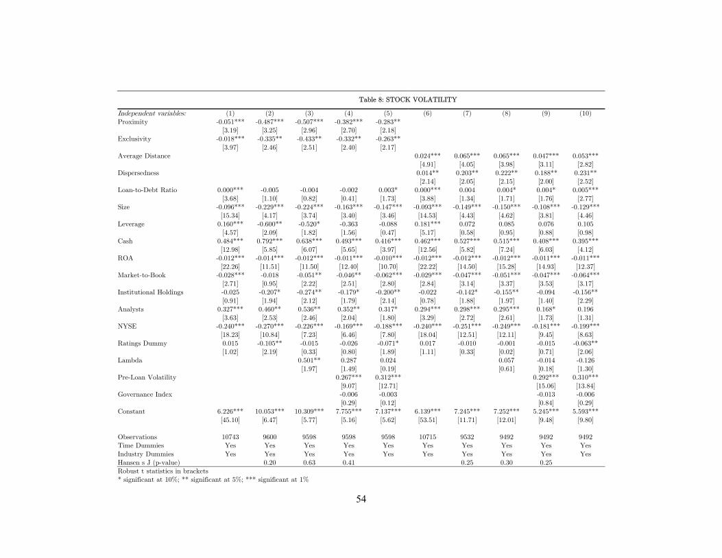
54

Table 8: STOCK VOLATILITY

Independent variables: (1) (2) (3) (4) (5) (6) (7) (8) (9) (10) Proximity -0.051*** -0.487*** -0.507*** -0.382*** -0.283** [3.19] [3.25] [2.96] [2.70] [2.18] Exclusivity -0.018*** -0.335** -0.433** -0.332** -0.263** [3.97] [2.46] [2.51] [2.40] [2.17] Average Distance 0.024*** 0.065*** 0.065*** 0.047*** 0.053*** [4.91] [4.05] [3.98] [3.11] [2.82] Dispersedness 0.014** 0.203** 0.222** 0.188** 0.231** [2.14] [2.05] [2.15] [2.00] [2.52] Loan-to-Debt Ratio 0.000*** -0.005 -0.004 -0.002 0.003* 0.000*** 0.004 0.004* 0.004* 0.005*** [3.68] [1.10] [0.82] [0.41] [1.73] [3.88] [1.34] [1.71] [1.76] [2.77] Size -0.096*** -0.229*** -0.224*** -0.163*** -0.147*** -0.093*** -0.149*** -0.150*** -0.108*** -0.129*** [15.34] [4.17] [3.74] [3.40] [3.46] [14.53] [4.43] [4.62] [3.81] [4.46] Leverage 0.160*** -0.600** -0.520* -0.363 -0.088 0.181*** 0.072 0.085 0.076 0.105 [4.57] [2.09] [1.82] [1.56] [0.47] [5.17] [0.58] [0.95] [0.88] [0.98] Cash 0.484*** 0.792*** 0.638*** 0.493*** 0.416*** 0.462*** 0.527*** 0.515*** 0.408*** 0.395*** [12.98] [5.85] [6.07] [5.65] [3.97] [12.56] [5.82] [7.24] [6.03] [4.12] ROA -0.012*** -0.014*** -0.012*** -0.011*** -0.010*** -0.012*** -0.012*** -0.012*** -0.011*** -0.011*** [22.26] [11.51] [11.50] [12.40] [10.70] [22.22] [14.50] [15.28] [14.93] [12.37] Market-to-Book -0.028*** -0.018 -0.051** -0.046** -0.062*** -0.029*** -0.047*** -0.051*** -0.047*** -0.064*** [2.71] [0.95] [2.22] [2.51] [2.80] [2.84] [3.14] [3.37] [3.53] [3.17] Institutional Holdings -0.025 -0.207* -0.274** -0.179* -0.200** -0.022 -0.142* -0.155** -0.094 -0.156** [0.91] [1.94] [2.12] [1.79] [2.14] [0.78] [1.88] [1.97] [1.40] [2.29] Analysts 0.327*** 0.460** 0.536** 0.352** 0.317* 0.294*** 0.298*** 0.295*** 0.168* 0.196 [3.63] [2.53] [2.46] [2.04] [1.80] [3.29] [2.72] [2.61] [1.73] [1.31] NYSE -0.240*** -0.270*** -0.226*** -0.169*** -0.188*** -0.240*** -0.251*** -0.249*** -0.181*** -0.199*** [18.23] [10.84] [7.23] [6.46] [7.80] [18.04] [12.51] [12.11] [9.45] [8.63] Ratings Dummy 0.015 -0.105** -0.015 -0.026 -0.071* 0.017 -0.010 -0.001 -0.015 -0.063** [1.02] [2.19] [0.33] [0.80] [1.89] [1.11] [0.33] [0.02] [0.71] [2.06] Lambda 0.501** 0.287 0.024 0.057 -0.014 -0.126 [1.97] [1.49] [0.19] [0.61] [0.18] [1.30] Pre-Loan Volatility 0.267*** 0.312*** 0.292*** 0.310*** [9.07] [12.71] [15.06] [13.84] Governance Index -0.006 -0.003 -0.013 -0.006 [0.29] [0.12] [0.84] [0.29] Constant 6.226*** 10.053*** 10.309*** 7.755*** 7.137*** 6.139*** 7.245*** 7.252*** 5.245*** 5.593*** [45.10] [6.47] [5.77] [5.16] [5.62] [53.51] [11.71] [12.01] [9.48] [9.80] Observations 10743 9600 9598 9598 9598 10715 9532 9492 9492 9492 Time Dummies Yes Yes Yes Yes Yes Yes Yes Yes Yes Yes Industry Dummies Yes Yes Yes Yes Yes Yes Yes Yes Yes Yes Hansen's J (p-value) 0.20 0.63 0.41 0.25 0.30 0.25 Robust t statistics in brackets * significant at 10%; ** significant at 5%; *** significant at 1%

55

Table 9

Lending relationship and cashflow variation This table examines how cashflow volatility of the borrowing firm changes with the characteristics of its bank loan. The dependent variable Cashflow Volatility is constructed in the following manner. It is the absolute change in cashflows with respect to the average cashflows over the previous three years. Our measure is in the same realm as the cashflow-shock measures of Guay and Harford (2000).

Our independent variables consist of loan characteristics and several firm-level control variables. We look at two complementary pairs of loan characteristics: either Proximity and Exclusivity or Average Distance and Dispersedness. Proximity is the fraction of loans taken from banks whose headquarters are located within 200 miles (or 320 kilometers) of the borrower’s location; historical location of the firm is available to us at county level so we also identify the banks’ location at county level. Exclusivity is the logarithm of the Herfindahl Index (ranging between 0—10,000) of the lending syndicate. Average Distance is the average distance of the borrower from each of the lenders in its lending syndicate; it is measured in thousands of kilometers. Dispersedness is the logarithm of the number of lenders counted in hundreds; this rescaling is done for the convenience of obtaining normally-scaled coefficient estimates. The results for the first pair (Proximity and Exclusivity) are in columns (1)-(5) and coefficient estimates using the second pair of characteristics (Average Distance and Dispersedness) are listed in columns (6)-(10). Columns (1) and (6) present OLS estimates while the remaining columns present results from an IV2SLS regression. Of the IV 2SLS regressions, columns (5) and (10) present the between-effects estimate. While our focus is on these loan characteristics, we also control for the Loan-to-Debt Ratio; it is measured as the ratio of firm’s total loan to outstanding long-term debt (item 9) in the previous fiscal year.

The firm-level control variables that we include in our analysis are the following. Size is measured as the logarithm of book value of assets (item 6). Leverage is the sum of long-

term debt (item 9) and debt in current liabilities (item 34), standardized by lagged assets (item 6). Cash is the ratio of total cash (item 1) to lagged assets and Cashflows are defined as income before extraordinary items (item 18) plus depreciation and amortization (item 14), standardized by lagged assets. We do not use ROA (return on assets) because it is important to control for the level of cashflows when explaining cashflow volatility, and moreover, there is a high correlation between Cashflows and ROA (97% in our data sample), so replacing ROA shouldn’t pose a problem. These firm-level variables are contemporaneous with the dependent variable while the remaining firm-characteristics are recorded at the beginning of the fiscal year. Market-to-Book is the logarithm of the firm’s market-to-book ratio where market-to-book is (item25 x item199)/(item60). Institutional Holdings is the fraction of shares held by those institutional investors that hold at least a 5% position in the firm. Analysts is the number of analysts following the stock, and is expressed in thousands for the convenience of obtaining normally-scaled coefficient estimates. NYSE is a dummy variable that takes a value 1 if the firm is listed on the New York Stock Exchange, and zero otherwise. Ratings Dummy is a dummy variable that equals one if the firm has a credit-rating, and equals zero otherwise.

Lambda — the inverse Mills’ ratio from the Probit analysis of loan-taking decision — is included in order to account for the selection bias inherent in our sample of loan-taking

firms. Pre-loan Cashflow Variation is the level of cashflow variation (our dependent variable in this table) in the year before the loan deal is initiated. Governance index is a dummy variable that equals 1 if the Gompers, Ishii, and Metrick (2003) index of corporate governance is greater than 9 and equals 0 if this index is less than or equal to 9; recall, the higher the index, the poorer the corporate governance. Industries are categorized by 1-digit SIC Code. The bottom row displays the p-value for Hansen’s J-test of the null hypothesis that the instrumental variables employed are orthogonal to the errors. All t-statistics are calculated using robust standard errors clustered at firm level.

56

Table 9: CASHFLOW VARIATION

Independent variables: (1) (2) (3) (4) (5) (6) (7) (8) (9) (10) Proximity -0.089 -1.931** -1.959* -2.002* -2.425** [1.14] [1.98] [1.83] [1.80] [2.03] Exclusivity -0.034 -2.279*** -2.675*** -2.702*** -2.783*** [1.59] [3.60] [3.29] [3.27] [3.10] Average Distance 0.091*** 0.218** 0.198** 0.208** 0.267** [3.88] [2.41] [2.15] [2.10] [2.52] Dispersedness 0.039 1.095*** 1.319*** 1.405*** 1.864*** [1.24] [2.66] [2.90] [2.93] [3.47] Loan-to-Debt Ratio -0.001 -0.023 -0.010 -0.012 -0.025 -0.001 -0.042* -0.046** -0.049** -0.001 [0.99] [0.85] [0.35] [0.41] [1.22] [0.95] [1.89] [2.16] [2.22] [0.12] Size -0.163*** -1.095*** -1.097*** -1.095*** -1.165*** -0.161*** -0.597*** -0.539*** -0.540*** -0.800*** [5.43] [4.38] [3.80] [3.80] [3.76] [5.21] [3.64] [3.66] [3.65] [4.76] Leverage -0.212 -4.785*** -4.480*** -4.472*** -4.699*** -0.183 -2.308*** -1.910*** -2.026*** -1.879*** [1.17] [3.77] [3.08] [3.00] [3.13] [1.02] [2.72] [3.25] [3.17] [2.94] Cash 0.784*** 2.319*** 1.725*** 1.793*** 2.941*** 0.714*** 2.024*** 1.648*** 1.738*** 2.327*** [3.38] [3.58] [2.96] [2.96] [3.25] [3.07] [3.42] [3.63] [3.56] [3.96] Cashflows -4.722*** -5.941*** -5.461*** -5.636*** -6.204*** -4.716*** -5.754*** -5.375*** -5.489*** -6.254*** [10.49] [7.92] [7.74] [7.72] [7.90] [10.46] [8.62] [9.05] [8.97] [12.43] Market-to-Book 0.040 0.145 0.030 0.043 -0.070 0.035 0.125 0.022 0.031 -0.063 [0.59] [1.13] [0.23] [0.33] [0.38] [0.52] [1.24] [0.23] [0.31] [0.54] Institutional Holdings -0.307** -1.809*** -2.118*** -2.082*** -1.686** -0.289** -0.795** -0.885*** -0.825** -1.089*** [2.14] [3.30] [3.39] [3.42] [2.49] [2.00] [2.52] [2.59] [2.48] [2.98] Analysts 0.215 1.704 1.929 1.659 1.729 0.106 0.349 0.430 0.361 0.392 [0.41] [1.64] [1.60] [1.40] [1.20] [0.21] [0.54] [0.63] [0.52] [0.45] NYSE -0.112* -0.372** -0.248 -0.256 -0.458** -0.123* -0.291*** -0.148 -0.125 -0.543*** [1.73] [2.58] [1.41] [1.39] [2.31] [1.91] [2.63] [1.12] [0.89] [4.07] Ratings Dummy 0.236*** -0.448* -0.149 -0.129 -0.719** 0.213*** -0.213 0.088 0.092 -0.478*** [3.62] [1.93] [0.66] [0.57] [2.34] [3.26] [1.21] [0.50] [0.51] [2.64] Lambda 1.513 1.509 0.862 1.690* 1.756* -0.969 [1.29] [1.26] [0.74] [1.65] [1.65] [1.63] Pre-Loan Cashflow Variation -0.004* -0.004 0.001 0.001 [1.80] [0.70] [0.32] [0.31] Governance Index 0.064 0.027 -0.034 -0.027 [0.43] [0.14] [0.38] [0.22] Constant 2.625*** 26.641*** 27.767*** 30.469*** 32.080*** 2.199*** 9.544*** 8.189*** 8.101*** 14.107*** [5.58] [4.02] [3.57] [3.59] [3.54] [6.01] [3.55] [3.33] [3.17] [4.83] Observations 10517 9412 9373 9373 9496 10491 9326 9324 9324 9324 Time Dummies Yes Yes Yes Yes Yes Yes Yes Yes Yes Yes Industry Dummies Yes Yes Yes Yes Yes Yes Yes Yes Yes Yes Hansen's J (p-value) 0.76 0.74 0.67 0.27 0.63 0.64 Robust t statistics in brackets * significant at 10%; ** significant at 5%; *** significant at 1%

57

Table 10

Lending relationship and managerial appropriation This table examines the impact of loan characteristics on potential appropriation of rents by managers. We measure Managerial Appropriation as the borrowing firm’s CEO’s total compensation as a fraction of the average CEO compensation for all firms (except the firm under consideration) in the corresponding industry.

Our independent variables consist of loan characteristics and several firm-level control variables. We look at two complementary pairs of loan characteristics: either Proximity and Exclusivity or Average Distance and Dispersedness. Proximity is the fraction of loans taken from banks whose headquarters are located within 200 miles (or 320 kilometers) of the borrower’s location; historical location of the firm is available to us at county level so we also identify the banks’ location at county level. Exclusivity is the logarithm of the Herfindahl Index (ranging between 0—10,000) of the lending syndicate. Average Distance is the average distance of the borrower from each of the lenders in its lending syndicate; it is measured in thousands of kilometers. Dispersedness is the logarithm of the number of lenders counted in hundreds; this rescaling is done for the convenience of obtaining normally-scaled coefficient estimates. The results for the first pair (Proximity and Exclusivity) are in columns (1)-(5) and coefficient estimates using the second pair of characteristics (Average Distance and Dispersedness) are listed in columns (6)-(10). Columns (1) and (6) present OLS estimates while the remaining columns present results from an IV2SLS regression. Of the IV 2SLS regressions, columns (5) and (10) present the between-effects estimate. While our focus is on these loan characteristics, we also control for the Loan-to-Debt Ratio; it is measured as the ratio of firm’s total loan to outstanding long-term debt (item 9) in the previous fiscal year.

The firm-level control variables that we include in our analysis are the following. Lagged CEO-Compensation is the logarithm of CEO’s total compensation (“TDC1” from

ExecuComp) in the previous fiscal year. Size is measured as the logarithm of book value of assets (item 6). Leverage is the sum of long-term debt (item 9) and debt in current liabilities (item 34), standardized by lagged assets (item 6). Cash is the ratio of total cash (item 1) to lagged assets and Cashflows are defined as income before extraordinary items (item 18) plus depreciation and amortization (item 14), standardized by lagged assets. We do not use ROA (return on assets) because it is important to control for the level of cashflows when explaining cashflow volatility, and moreover, there is a high correlation between Cashflows and ROA (97% in our data sample), so replacing ROA shouldn’t pose a problem. These firm-level variables are contemporaneous with the dependent variable while the remaining firm-characteristics are recorded at the beginning of the fiscal year. Market-to-Book is the logarithm of the firm’s market-to-book ratio where market-to-book is (item25 x item199)/(item60). Institutional Holdings is the fraction of shares held by those institutional investors that hold at least a 5% position in the firm. Analysts is the number of analysts following the stock, and is expressed in thousands for the convenience of obtaining normally-scaled coefficient estimates. NYSE is a dummy variable that takes a value 1 if the firm is listed on the New York Stock Exchange, and zero otherwise. Ratings Dummy is a dummy variable that equals one if the firm has a credit-rating, and equals zero otherwise.

Lambda — the inverse Mills’ ratio from the Probit analysis of loan-taking decision — is included in order to account for the selection bias inherent in our sample of loan-taking

firms. Lagged Appropriation is the level of managerial appropriation (our dependent variable in this table) in the previous fiscal year; we do not use the pre-loan figure in this case because the CEO could be different before the loan starts. Governance index is a dummy variable that equals 1 if the Gompers, Ishii, and Metrick (2003) index of corporate governance is greater than 9 and equals 0 if this index is less than or equal to 9; recall, the higher the index, the poorer the corporate governance. Industries are categorized by 1-digit SIC Code. The bottom row displays the p-value for Hansen’s J-test of the null hypothesis that the instrumental variables employed are orthogonal to the errors. All t-statistics are calculated using robust standard errors clustered at firm level.

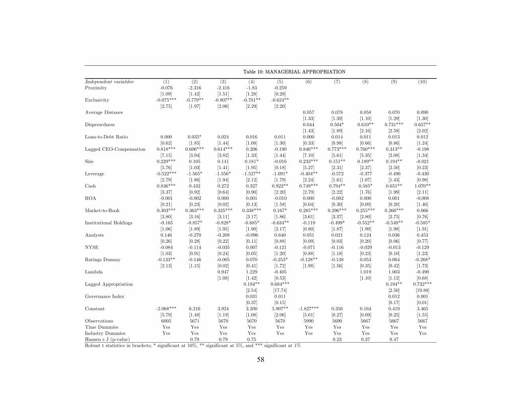
58

Table 10: MANAGERIAL APPROPRIATION

Independent variables: (1) (2) (3) (4) (5) (6) (7) (8) (9) (10) Proximity -0.076 -2.316 -2.416 -1.83 -0.259 [1.09] [1.42] [1.51] [1.28] [0.29] Exclusivity -0.075*** -0.779** -0.807** -0.781** -0.624** [2.75] [1.97] [2.06] [2.29] [2.20] Average Distance 0.057 0.078 0.058 0.070 0.090 [1.33] [1.39] [1.10] [1.29] [1.30] Dispersedness 0.044 0.504* 0.610** 0.731*** 0.657** [1.43] [1.89] [2.16] [2.58] [2.02] Loan-to-Debt Ratio 0.000 0.035* 0.024 0.016 0.011 0.000 0.014 0.011 0.013 0.012 [0.62] [1.85] [1.44] [1.08] [1.30] [0.33] [0.98] [0.66] [0.86] [1.24] Lagged CEO-Compensation 0.818*** 0.606*** 0.614*** 0.206 -0.190 0.846*** 0.773*** 0.760*** 0.313** -0.198 [7.15] [3.94] [3.82] [1.33] [1.44] [7.10] [5.61] [5.35] [2.08] [1.34] Size 0.229*** 0.105 0.141 0.181* -0.016 0.233*** 0.151** 0.189** 0.194** -0.021 [5.76] [1.03] [1.41] [1.95] [0.18] [5.27] [2.31] [2.37] [2.50] [0.23] Leverage -0.522*** -1.565* -1.556* -1.527** -1.091* -0.404** -0.572 -0.377 -0.496 -0.430 [2.79] [1.86] [1.94] [2.12] [1.79] [2.24] [1.61] [1.07] [1.43] [0.98] Cash 0.836*** 0.432 0.272 0.327 0.922** 0.749*** 0.794** 0.585* 0.651** 1.070** [3.37] [0.92] [0.64] [0.90] [2.20] [2.79] [2.22] [1.76] [1.99] [2.11] ROA -0.001 -0.002 0.000 0.001 -0.010 0.000 -0.002 0.000 0.001 -0.008 [0.21] [0.23] [0.02] [0.13] [1.58] [0.04] [0.30] [0.09] [0.20] [1.40] Market-to-Book 0.303*** 0.363*** 0.335*** 0.338*** 0.167* 0.285*** 0.296*** 0.255*** 0.266*** 0.066 [3.80] [3.16] [3.11] [3.17] [1.86] [3.61] [3.37] [2.80] [2.75] [0.76] Institutional Holdings -0.165 -0.857* -0.828* -0.685* -0.634** -0.119 -0.499* -0.552** -0.540** -0.585* [1.06] [1.89] [1.95] [1.90] [2.17] [0.80] [1.87] [1.99] [1.98] [1.91] Analysts 0.146 -0.270 -0.208 -0.096 0.640 0.051 0.021 0.124 0.036 0.453 [0.26] [0.28] [0.22] [0.11] [0.88] [0.09] [0.03] [0.20] [0.06] [0.77] NYSE -0.084 -0.114 -0.035 0.007 -0.121 -0.071 -0.116 -0.029 -0.013 -0.129 [1.03] [0.91] [0.24] [0.05] [1.20] [0.88] [1.18] [0.23] [0.10] [1.23] Ratings Dummy -0.133** -0.146 -0.005 0.070 -0.253* -0.128** -0.138 0.053 0.064 -0.268* [2.13] [1.15] [0.02] [0.41] [1.72] [1.98] [1.56] [0.35] [0.42] [1.73] Lambda 0.947 1.229 -0.405 1.019 1.003 -0.490 [1.08] [1.42] [0.53] [1.10] [1.12] [0.68] Lagged Appropriation 0.194** 0.684*** 0.194** 0.732*** [2.54] [17.74] [2.50] [19.88] Governance Index 0.031 0.011 0.012 0.001 [0.37] [0.15] [0.17] [0.01] Constant -2.068*** 6.216 3.924 3.200 5.907** -1.827*** 0.356 0.164 0.419 3.465 [5.79] [1.48] [1.19] [1.08] [2.06] [5.01] [0.27] [0.09] [0.25] [1.55] Observations 6005 5671 5670 5670 5670 5990 5690 5667 5667 5667 Time Dummies Yes Yes Yes Yes Yes Yes Yes Yes Yes Yes Industry Dummies Yes Yes Yes Yes Yes Yes Yes Yes Yes Yes Hansen's J (p-value) 0.79 0.79 0.75 0.23 0.37 0.47 Robust t statistics in brackets; * significant at 10%, ** significant at 5%, and *** significant at 1%

59

Table 11

Lending relationship and trading by managers

This table examines the impact of loan characteristics on the trading behavior of borrowing firm’s managers. More specifically, we measure Trading by Managers as the ratio of the borrowing firm’s CEO’s trades to the average trading by CEOs of all firms (except the firm under consideration) in the corresponding industry; we calculate CEO’s trades according to Jenter (2005).

Our independent variables consist of loan characteristics and several firm-level control variables. We look at two complementary pairs of loan characteristics: either Proximity and Exclusivity or Average Distance and Dispersedness. Proximity is the fraction of loans taken from banks whose headquarters are located within 200 miles (or 320 kilometers) of the borrower’s location; historical location of the firm is available to us at county level so we also identify the banks’ location at county level. Exclusivity is the logarithm of the Herfindahl Index (ranging between 0—10,000) of the lending syndicate. Average Distance is the average distance of the borrower from each of the lenders in its lending syndicate; it is measured in thousands of kilometers. Dispersedness is the logarithm of the number of lenders counted in hundreds; this rescaling is done for the convenience of obtaining normally-scaled coefficient estimates. The results for the first pair (Proximity and Exclusivity) are in columns (1)-(5) and coefficient estimates using the second pair of characteristics (Average Distance and Dispersedness) are listed in columns (6)-(10). Columns (1) and (6) present OLS estimates while the remaining columns present results from an IV2SLS regression. Of the IV 2SLS regressions, columns (5) and (10) present the between-effects estimate. While our focus is on these loan characteristics, we also control for the Loan-to-Debt Ratio; it is measured as the ratio of firm’s total loan to outstanding long-term debt (item 9) in the previous fiscal year.

The firm-level control variables that we include in our analysis are the following. Lagged CEO-Compensation is the logarithm of CEO’s total compensation (“TDC1” from

ExecuComp) in the previous fiscal year. Size is measured as the logarithm of book value of assets (item 6). Leverage is the sum of long-term debt (item 9) and debt in current liabilities (item 34), standardized by lagged assets (item 6). Cash is the ratio of total cash (item 1) to lagged assets and Cashflows are defined as income before extraordinary items (item 18) plus depreciation and amortization (item 14), standardized by lagged assets. We do not use ROA (return on assets) because it is important to control for the level of cashflows when explaining cashflow volatility, and moreover, there is a high correlation between Cashflows and ROA (97% in our data sample), so replacing ROA shouldn’t pose a problem. These firm-level variables are contemporaneous with the dependent variable while the remaining firm-characteristics are recorded at the beginning of the fiscal year. Market-to-Book is the logarithm of the firm’s market-to-book ratio where market-to-book is (item25 x item199)/(item60). Institutional Holdings is the fraction of shares held by those institutional investors that hold at least a 5% position in the firm. Analysts is the number of analysts following the stock, and is expressed in thousands for the convenience of obtaining normally-scaled coefficient estimates. NYSE is a dummy variable that takes a value 1 if the firm is listed on the New York Stock Exchange, and zero otherwise. Ratings Dummy is a dummy variable that equals one if the firm has a credit-rating, and equals zero otherwise.

Lambda — the inverse Mills’ ratio from the Probit analysis of loan-taking decision — is included in order to account for the selection bias inherent in our sample of loan-taking

firms. Lagged CEO-trading is the level of trading by managers (our dependent variable in this table) in the previous fiscal year; we do not use the pre-loan figure in this case because the CEO could be different before the loan starts. Governance index is a dummy variable that equals 1 if the Gompers, Ishii, and Metrick (2003) index of corporate governance is greater than 9 and equals 0 if this index is less than or equal to 9; recall, the higher the index, the poorer the corporate governance. Industries are categorized by 1-digit SIC Code. The bottom row displays the p-value for Hansen’s J-test of the null hypothesis that the instrumental variables employed are orthogonal to the errors. All t-statistics are calculated using robust standard errors clustered at firm level.

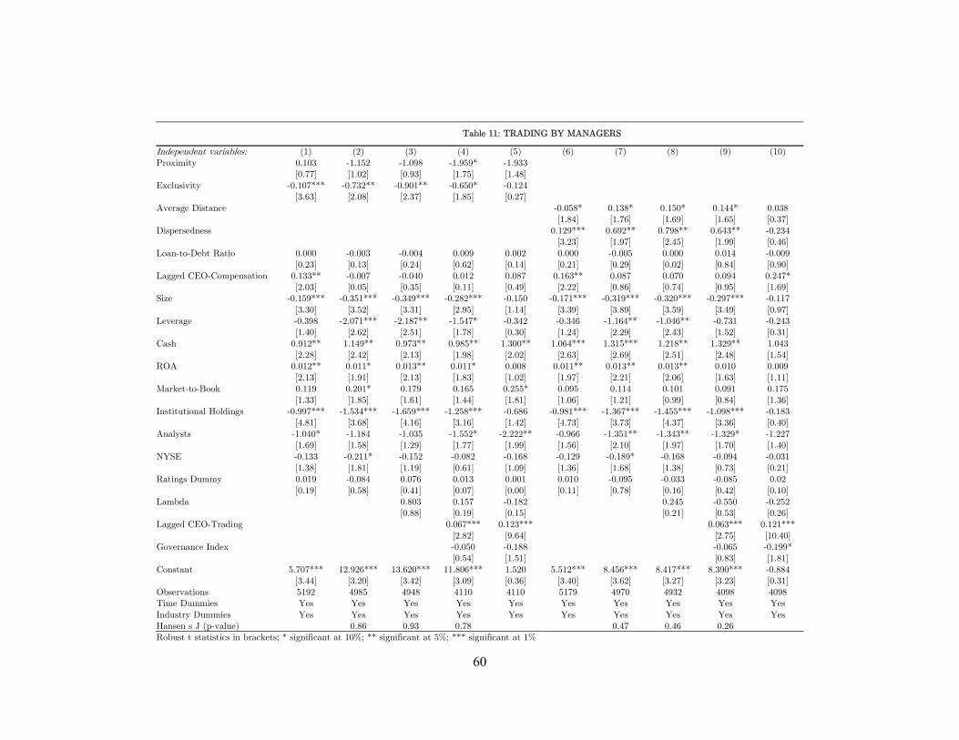
60

Table 11: TRADING BY MANAGERS

Independent variables: (1) (2) (3) (4) (5) (6) (7) (8) (9) (10) Proximity 0.103 -1.152 -1.098 -1.959* -1.933 [0.77] [1.02] [0.93] [1.75] [1.48] Exclusivity -0.107*** -0.732** -0.901** -0.650* -0.124 [3.63] [2.08] [2.37] [1.85] [0.27] Average Distance -0.058* 0.138* 0.150* 0.144* 0.038 [1.84] [1.76] [1.69] [1.65] [0.37] Dispersedness 0.129*** 0.692** 0.798** 0.643** -0.234 [3.23] [1.97] [2.45] [1.99] [0.46] Loan-to-Debt Ratio 0.000 -0.003 -0.004 0.009 0.002 0.000 -0.005 0.000 0.014 -0.009 [0.23] [0.13] [0.24] [0.62] [0.14] [0.21] [0.29] [0.02] [0.84] [0.90] Lagged CEO-Compensation 0.133** -0.007 -0.040 0.012 0.087 0.163** 0.087 0.070 0.094 0.247* [2.03] [0.05] [0.35] [0.11] [0.49] [2.22] [0.86] [0.74] [0.95] [1.69] Size -0.159*** -0.351*** -0.349*** -0.282*** -0.150 -0.171*** -0.319*** -0.320*** -0.297*** -0.117 [3.30] [3.52] [3.31] [2.95] [1.14] [3.39] [3.89] [3.59] [3.49] [0.97] Leverage -0.398 -2.071*** -2.187** -1.547* -0.342 -0.346 -1.164** -1.046** -0.731 -0.243 [1.40] [2.62] [2.51] [1.78] [0.30] [1.24] [2.29] [2.43] [1.52] [0.31] Cash 0.912** 1.149** 0.973** 0.985** 1.300** 1.064*** 1.315*** 1.218** 1.329** 1.043 [2.28] [2.42] [2.13] [1.98] [2.02] [2.63] [2.69] [2.51] [2.48] [1.54] ROA 0.012** 0.011* 0.013** 0.011* 0.008 0.011** 0.013** 0.013** 0.010 0.009 [2.13] [1.91] [2.13] [1.83] [1.02] [1.97] [2.21] [2.06] [1.63] [1.11] Market-to-Book 0.119 0.201* 0.179 0.165 0.255* 0.095 0.114 0.101 0.091 0.175 [1.33] [1.85] [1.61] [1.44] [1.81] [1.06] [1.21] [0.99] [0.84] [1.36] Institutional Holdings -0.997*** -1.534*** -1.659*** -1.258*** -0.686 -0.981*** -1.367*** -1.455*** -1.098*** -0.183 [4.81] [3.68] [4.16] [3.16] [1.42] [4.73] [3.73] [4.37] [3.36] [0.40] Analysts -1.040* -1.184 -1.035 -1.552* -2.222** -0.966 -1.351** -1.343** -1.329* -1.227 [1.69] [1.58] [1.29] [1.77] [1.99] [1.56] [2.10] [1.97] [1.70] [1.40] NYSE -0.133 -0.211* -0.152 -0.082 -0.168 -0.129 -0.189* -0.168 -0.094 -0.031 [1.38] [1.81] [1.19] [0.61] [1.09] [1.36] [1.68] [1.38] [0.73] [0.21] Ratings Dummy 0.019 -0.084 0.076 0.013 0.001 0.010 -0.095 -0.033 -0.085 0.02 [0.19] [0.58] [0.41] [0.07] [0.00] [0.11] [0.78] [0.16] [0.42] [0.10] Lambda 0.803 0.157 -0.182 0.245 -0.550 -0.252 [0.88] [0.19] [0.15] [0.21] [0.53] [0.26] Lagged CEO-Trading 0.067*** 0.123*** 0.063*** 0.121*** [2.82] [9.64] [2.75] [10.40] Governance Index -0.050 -0.188 -0.065 -0.199* [0.54] [1.51] [0.83] [1.81] Constant 5.707*** 12.926*** 13.620*** 11.806*** 1.520 5.512*** 8.456*** 8.417*** 8.390*** -0.884 [3.44] [3.20] [3.42] [3.09] [0.36] [3.40] [3.62] [3.27] [3.23] [0.31] Observations 5192 4985 4948 4110 4110 5179 4970 4932 4098 4098 Time Dummies Yes Yes Yes Yes Yes Yes Yes Yes Yes Yes Industry Dummies Yes Yes Yes Yes Yes Yes Yes Yes Yes Yes Hansen's J (p-value) 0.86 0.93 0.78 0.47 0.46 0.26 Robust t statistics in brackets; * significant at 10%; ** significant at 5%; *** significant at 1%

61

Table 12

Lending relationship and expenditure on M&As This table presents coefficient estimates for the relationship between the loan characteristics and the amount spent by the borrowing firm’s managers on acquisitions. The dependent variable in this case is measured as the ratio of Compustat item 129 to lagged assets.

Our independent variables consist of loan characteristics and several firm-level control variables. We look at two complementary pairs of loan characteristics: either Proximity and Exclusivity or Average Distance and Dispersedness. Proximity is the fraction of loans taken from banks whose headquarters are located within 200 miles (or 320 kilometers) of the borrower’s location; historical location of the firm is available to us at county level so we also identify the banks’ location at county level. Exclusivity is the logarithm of the Herfindahl Index (ranging between 0—10,000) of the lending syndicate. Average Distance is the average distance of the borrower from each of the lenders in its lending syndicate; it is measured in thousands of kilometers. Dispersedness is the logarithm of the number of lenders counted in hundreds; this rescaling is done for the convenience of obtaining normally-scaled coefficient estimates. The results for the first pair (Proximity and Exclusivity) are in columns (1)-(5) and coefficient estimates using the second pair of characteristics (Average Distance and Dispersedness) are listed in columns (6)-(10). Columns (1) and (6) present OLS estimates while the remaining columns present results from an IV2SLS regression. Of the IV 2SLS regressions, columns (5) and (10) present the between-effects estimate. While our focus is on these loan characteristics, we also control for the Loan-to-Debt Ratio; it is measured as the ratio of firm’s total loan to outstanding long-term debt (item 9) in the previous fiscal year.

The firm-level control variables that we include in our analysis are the following. Size is measured as the logarithm of book value of assets (item 6). Leverage is the sum of long-

term debt (item 9) and debt in current liabilities (item 34), standardized by lagged assets (item 6). Cash is the ratio of total cash (item 1) to lagged assets and the ROA (return on assets) is income before extraordinary items (item 18) as a percentage of lagged assets. These firm-level variables are contemporaneous with the dependent variable while the remaining firm-characteristics are recorded at the beginning of the fiscal year. Market-to-Book is the logarithm of the firm’s market-to-book ratio where market-to-book is (item25 x item199)/(item60). Institutional Holdings is the fraction of shares held by those institutional investors that hold at least a 5% position in the firm. Analysts is the number of analysts following the stock, and is expressed in thousands for the convenience of obtaining normally-scaled coefficient estimates. NYSE is a dummy variable that takes a value 1 if the firm is listed on the New York Stock Exchange, and zero otherwise. Ratings Dummy is a dummy variable that equals one if the firm has a credit-rating, and equals zero otherwise.

Lambda — the inverse Mills’ ratio from the Probit analysis of loan-taking decision — is included in order to account for the selection bias inherent in our sample of loan-taking

firms. Pre-loan Expenditure on M&A is the level of M&A expenditure (our dependent variable in this table) in the year before the loan deal is initiated. Governance index is a dummy variable that equals 1 if the Gompers, Ishii, and Metrick (2003) index of corporate governance is greater than 9 and equals 0 if this index is less than or equal to 9; recall, the higher the index, the poorer the corporate governance. Industries are categorized by 1-digit SIC Code. The bottom row displays the p-value for Hansen’s J-test of the null hypothesis that the instrumental variables employed are orthogonal to the errors. All t-statistics are calculated using robust standard errors clustered at firm level.

62

Table 12: EXPENDITURE ON M&As

Independent variables: (1) (2) (3) (4) (5) (6) (7) (8) (9) (10) Proximity -0.002 -0.063 -0.084 -0.134 0.024 [0.40] [0.94] [0.93] [1.47] [0.45] Exclusivity -0.007*** -0.117** -0.171** -0.181** -0.106** [4.26] [2.16] [2.15] [2.09] [2.20] Average Distance -0.002 0.006 -0.006 -0.002 -0.009 [1.32] [1.20] [0.84] [0.24] [1.24] Dispersedness 0.009*** 0.099** 0.141*** 0.172** 0.113*** [4.34] [2.57] [2.94] [2.38] [2.99] Loan-to-Debt Ratio 0.000*** 0.006*** 0.009*** 0.008*** 0.002** 0.000*** 0.000 0.000 0.001 0.001 [5.90] [2.93] [3.58] [3.25] [2.39] [5.89] [0.08] [0.02] [0.54] [1.36] Size 0.005*** -0.028 -0.032 -0.038 -0.008 0.005** -0.027** -0.006 -0.016 -0.005 [2.71] [1.39] [1.13] [1.22] [0.47] [2.48] [2.01] [0.41] [0.70] [0.43] Leverage 0.153*** 0.145 0.187 0.147 0.175** 0.160*** 0.073* 0.217*** 0.181*** 0.190*** [10.63] [1.44] [1.41] [1.03] [2.37] [10.90] [1.72] [3.82] [2.71] [4.50] Cash 0.016 -0.026 -0.099 -0.090 -0.153*** 0.020 0.090** -0.024 -0.006 -0.092** [1.02] [0.49] [1.60] [1.37] [3.38] [1.26] [2.56] [0.58] [0.12] [2.27] ROA 0.001*** 0.002*** 0.003*** 0.002*** 0.001*** 0.001*** 0.001*** 0.002*** 0.002*** 0.001*** [5.98] [3.22] [3.42] [3.00] [3.17] [5.95] [4.12] [5.82] [4.86] [3.35] Market-to-Book 0.032*** 0.024** 0.010 0.012 0.030*** 0.032*** 0.032*** 0.007 0.007 0.027*** [5.70] [2.43] [0.79] [0.95] [3.12] [5.74] [4.83] [0.77] [0.67] [3.40] Institutional Holdings 0.029*** -0.084* -0.134** -0.111* -0.021 0.030*** -0.025 -0.044 -0.046 -0.003 [3.42] [1.67] [1.99] [1.65] [0.57] [3.39] [0.88] [1.33] [1.06] [0.10] Analysts -0.207*** -0.140* -0.102 -0.081 -0.159** -0.209*** -0.192*** -0.160*** -0.130** -0.178*** [6.40] [1.73] [0.90] [0.71] [1.99] [6.45] [4.59] [3.33] [2.30] [3.03] NYSE -0.019*** -0.028** -0.014 -0.008 -0.010 -0.020*** -0.034*** 0.002 0.005 -0.012 [4.27] [2.50] [0.92] [0.48] [0.97] [4.37] [4.16] [0.15] [0.35] [1.38] Ratings Dummy -0.002 0.001 0.035* 0.034* 0.031** -0.001 -0.022** 0.061*** 0.051** 0.035*** [0.52] [0.06] [1.76] [1.73] [2.07] [0.32] [2.24] [2.61] [2.27] [2.91] Lambda 0.165* 0.184** 0.222*** 0.415*** 0.367*** 0.242*** [1.81] [2.13] [4.23] [3.53] [3.30] [6.21] Pre-Loan Expenditure on M&A -0.013 -0.006 -0.004 -0.001 [1.41] [0.78] [0.74] [0.26] Governance Index 0.015 0.016 0.005 0.006 [1.02] [1.43] [0.61] [0.70] Constant -0.041* 1.040* 1.284 1.355 0.577 -0.034 0.518** 0.031 0.313 0.157 [1.67] [1.79] [1.60] [1.56] [1.14] [1.07] [2.14] [0.10] [0.80] [0.68] Observations 10164 9063 9060 8503 8503 10137 9488 9404 8614 8406 Time Dummies Yes Yes Yes Yes Yes Yes Yes Yes Yes Yes Industry Dummies Yes Yes Yes Yes Yes Yes Yes Yes Yes Yes Hansen's J (p-value) 0.86 0.76 0.94 0.21 0.23 0.52 Robust t statistics in brackets * significant at 10%; ** significant at 5%; *** significant at 1%

63

Table 13

Lending relationship and CEO turnover This table presents coefficient estimates for the relationship between the loan characteristics and the probability of CEO-turnover at the borrowing firm. Thus, the dependent variable in this case is simply a dummy that takes value 1 if the CEO changes in the given fiscal year, and 0 otherwise.

Our independent variables consist of loan characteristics and several firm-level control variables. We look at two complementary pairs of loan characteristics: either Proximity and Exclusivity or Average Distance and Dispersedness. Proximity is the fraction of loans taken from banks whose headquarters are located within 200 miles (or 320 kilometers) of the borrower’s location; historical location of the firm is available to us at county level so we also identify the banks’ location at county level. Exclusivity is the logarithm of the Herfindahl Index (ranging between 0—10,000) of the lending syndicate. Average Distance is the average distance of the borrower from each of the lenders in its lending syndicate; it is measured in thousands of kilometers. Dispersedness is the logarithm of the number of lenders counted in hundreds; this rescaling is done for the convenience of obtaining normally-scaled coefficient estimates. The results for the first pair (Proximity and Exclusivity) are in columns (1)-(5) and coefficient estimates using the second pair of characteristics (Average Distance and Dispersedness) are listed in columns (6)-(10). Columns (1) and (6) present OLS estimates while the remaining columns present results from an IV2SLS regression. Of the IV 2SLS regressions, columns (5) and (10) present the between-effects estimate. While our focus is on these loan characteristics, we also control for the Loan-to-Debt Ratio; it is measured as the ratio of firm’s total loan to outstanding long-term debt (item 9) in the previous fiscal year.

The firm-level control variables that we include in our analysis are the following. Size is measured as the logarithm of book value of assets (item 6). Leverage is the sum of long-

term debt (item 9) and debt in current liabilities (item 34), standardized by lagged assets (item 6). Cash is the ratio of total cash (item 1) to lagged assets and the ROA (return on assets) is income before extraordinary items (item 18) as a percentage of lagged assets. These firm-level variables are contemporaneous with the dependent variable. ROA in year (t-1) is the first lag of ROA and ROA in year (t-2) is the second lag of ROA. The remaining firm-characteristics are recorded at the beginning of the fiscal year. Market-to-Book is the logarithm of the firm’s market-to-book ratio where market-to-book is (item25 x item199)/(item60). Institutional Holdings is the fraction of shares held by those institutional investors that hold at least a 5% position in the firm. Analysts is the number of analysts following the stock, and is expressed in thousands for the convenience of obtaining normally-scaled coefficient estimates. NYSE is a dummy variable that takes a value 1 if the firm is listed on the New York Stock Exchange, and zero otherwise. Ratings Dummy is a dummy variable that equals one if the firm has a credit-rating, and equals zero otherwise.

Lambda — the inverse Mills’ ratio from the Probit analysis of loan-taking decision — is included in order to account for the selection bias inherent in our sample of loan-taking

firms. Governance index is a dummy variable that equals 1 if the Gompers, Ishii, and Metrick (2003) index of corporate governance is greater than 9 and equals 0 if this index is less than or equal to 9; recall, the higher the index, the poorer the corporate governance. Industries are categorized by 1-digit SIC Code. The bottom row displays the p-value for Hansen’s J-test of the null hypothesis that the instrumental variables employed are orthogonal to the errors. All t-statistics are calculated using robust standard errors clustered at firm level.

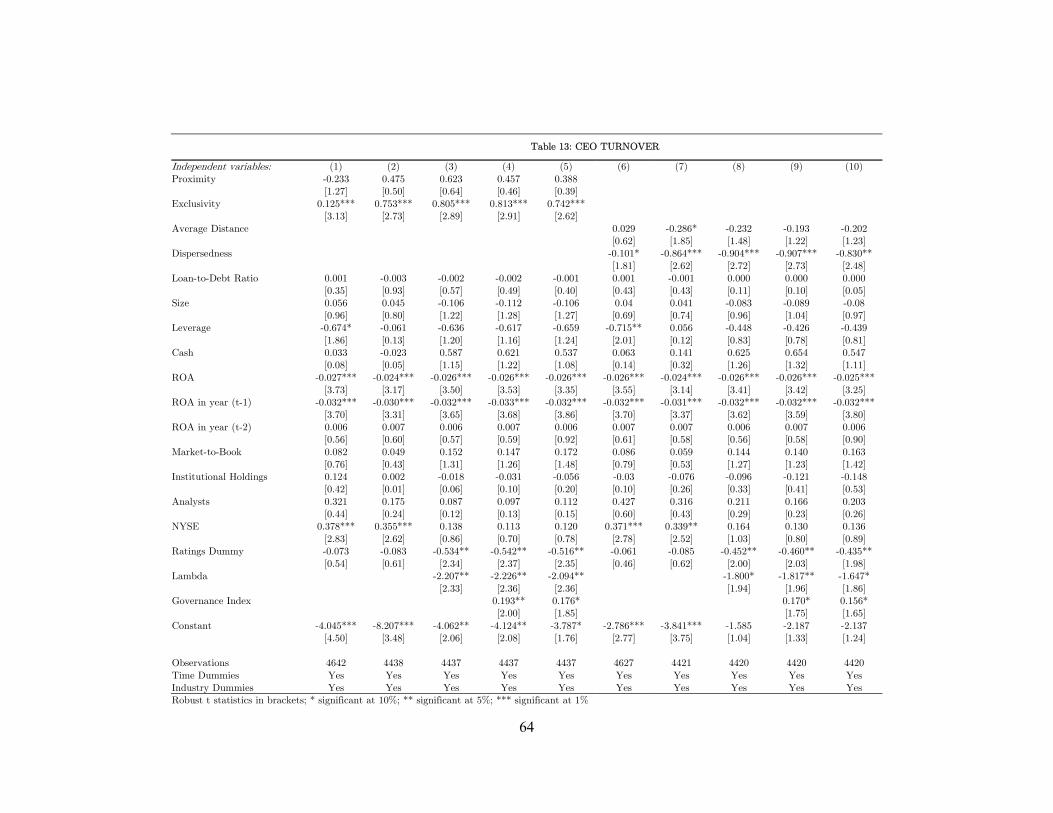
64

Table 13: CEO TURNOVER

Independent variables: (1) (2) (3) (4) (5) (6) (7) (8) (9) (10) Proximity -0.233 0.475 0.623 0.457 0.388 [1.27] [0.50] [0.64] [0.46] [0.39] Exclusivity 0.125*** 0.753*** 0.805*** 0.813*** 0.742*** [3.13] [2.73] [2.89] [2.91] [2.62] Average Distance 0.029 -0.286* -0.232 -0.193 -0.202 [0.62] [1.85] [1.48] [1.22] [1.23] Dispersedness -0.101* -0.864*** -0.904*** -0.907*** -0.830** [1.81] [2.62] [2.72] [2.73] [2.48] Loan-to-Debt Ratio 0.001 -0.003 -0.002 -0.002 -0.001 0.001 -0.001 0.000 0.000 0.000 [0.35] [0.93] [0.57] [0.49] [0.40] [0.43] [0.43] [0.11] [0.10] [0.05] Size 0.056 0.045 -0.106 -0.112 -0.106 0.04 0.041 -0.083 -0.089 -0.08 [0.96] [0.80] [1.22] [1.28] [1.27] [0.69] [0.74] [0.96] [1.04] [0.97] Leverage -0.674* -0.061 -0.636 -0.617 -0.659 -0.715** 0.056 -0.448 -0.426 -0.439 [1.86] [0.13] [1.20] [1.16] [1.24] [2.01] [0.12] [0.83] [0.78] [0.81] Cash 0.033 -0.023 0.587 0.621 0.537 0.063 0.141 0.625 0.654 0.547 [0.08] [0.05] [1.15] [1.22] [1.08] [0.14] [0.32] [1.26] [1.32] [1.11] ROA -0.027*** -0.024*** -0.026*** -0.026*** -0.026*** -0.026*** -0.024*** -0.026*** -0.026*** -0.025*** [3.73] [3.17] [3.50] [3.53] [3.35] [3.55] [3.14] [3.41] [3.42] [3.25] ROA in year (t-1) -0.032*** -0.030*** -0.032*** -0.033*** -0.032*** -0.032*** -0.031*** -0.032*** -0.032*** -0.032*** [3.70] [3.31] [3.65] [3.68] [3.86] [3.70] [3.37] [3.62] [3.59] [3.80] ROA in year (t-2) 0.006 0.007 0.006 0.007 0.006 0.007 0.007 0.006 0.007 0.006 [0.56] [0.60] [0.57] [0.59] [0.92] [0.61] [0.58] [0.56] [0.58] [0.90] Market-to-Book 0.082 0.049 0.152 0.147 0.172 0.086 0.059 0.144 0.140 0.163 [0.76] [0.43] [1.31] [1.26] [1.48] [0.79] [0.53] [1.27] [1.23] [1.42] Institutional Holdings 0.124 0.002 -0.018 -0.031 -0.056 -0.03 -0.076 -0.096 -0.121 -0.148 [0.42] [0.01] [0.06] [0.10] [0.20] [0.10] [0.26] [0.33] [0.41] [0.53] Analysts 0.321 0.175 0.087 0.097 0.112 0.427 0.316 0.211 0.166 0.203 [0.44] [0.24] [0.12] [0.13] [0.15] [0.60] [0.43] [0.29] [0.23] [0.26] NYSE 0.378*** 0.355*** 0.138 0.113 0.120 0.371*** 0.339** 0.164 0.130 0.136 [2.83] [2.62] [0.86] [0.70] [0.78] [2.78] [2.52] [1.03] [0.80] [0.89] Ratings Dummy -0.073 -0.083 -0.534** -0.542** -0.516** -0.061 -0.085 -0.452** -0.460** -0.435** [0.54] [0.61] [2.34] [2.37] [2.35] [0.46] [0.62] [2.00] [2.03] [1.98] Lambda -2.207** -2.226** -2.094** -1.800* -1.817** -1.647* [2.33] [2.36] [2.36] [1.94] [1.96] [1.86] Governance Index 0.193** 0.176* 0.170* 0.156* [2.00] [1.85] [1.75] [1.65] Constant -4.045*** -8.207*** -4.062** -4.124** -3.787* -2.786*** -3.841*** -1.585 -2.187 -2.137 [4.50] [3.48] [2.06] [2.08] [1.76] [2.77] [3.75] [1.04] [1.33] [1.24] Observations 4642 4438 4437 4437 4437 4627 4421 4420 4420 4420 Time Dummies Yes Yes Yes Yes Yes Yes Yes Yes Yes Yes Industry Dummies Yes Yes Yes Yes Yes Yes Yes Yes Yes Yes Robust t statistics in brackets; * significant at 10%; ** significant at 5%; *** significant at 1%

65

Table 14

Lending relationship and Tobin’s Q This table examines the relationship between the loan characteristics and firm value, as captured by Tobin’s Q. Tobin’s Q is calculated as (item6 + item25 x item199 — item60 — item74)/(item6).

Our independent variables consist of loan characteristics and several firm-level control variables. We look at two complementary pairs of loan characteristics: either Proximity and Exclusivity or Average Distance and Dispersedness. Proximity is the fraction of loans taken from banks whose headquarters are located within 200 miles (or 320 kilometers) of the borrower’s location; historical location of the firm is available to us at county level so we also identify the banks’ location at county level. Exclusivity is the logarithm of the Herfindahl Index (ranging between 0—10,000) of the lending syndicate. Average Distance is the average distance of the borrower from each of the lenders in its lending syndicate; it is measured in thousands of kilometers. Dispersedness is the logarithm of the number of lenders counted in hundreds; this rescaling is done for the convenience of obtaining normally-scaled coefficient estimates. The results for the first pair (Proximity and Exclusivity) are in columns (1)-(5) and coefficient estimates using the second pair of characteristics (Average Distance and Dispersedness) are listed in columns (6)-(10). Columns (1) and (6) present OLS estimates while the remaining columns present results from an IV2SLS regression. Of the IV 2SLS regressions, columns (5) and (10) present the between-effects estimate. While our focus is on these loan characteristics, we also control for the Loan-to-Debt Ratio; it is measured as the ratio of firm’s total loan to outstanding long-term debt (item 9) in the previous fiscal year.

The firm-level control variables that we include in our analysis are the following. Size is measured as the logarithm of book value of assets (item 6). Leverage is the sum of long-

term debt (item 9) and debt in current liabilities (item 34), standardized by lagged assets (item 6). Cash is the ratio of total cash (item 1) to lagged assets and the ROA (return on assets) is income before extraordinary items (item 18) as a percentage of lagged assets. Capital Expenditure is capital expenditure (item 128) as a fraction of lagged assets. Industry Tobin’s Q is the average Q in the industry to which the borrowing firm belongs. These firm-level variables are contemporaneous with the dependent variable while the remaining firm-characteristics are recorded at the beginning of the fiscal year. Lagged Tobin’s Q is the first lag of Tobin’s Q, our dependent variable in this table. Institutional Holdings is the fraction of shares held by those institutional investors that hold at least a 5% position in the firm. Analysts is the number of analysts following the stock, and is expressed in thousands for the convenience of obtaining normally-scaled coefficient estimates. NYSE is a dummy variable that takes a value 1 if the firm is listed on the New York Stock Exchange, and zero otherwise. Ratings Dummy is a dummy variable that equals one if the firm has a credit-rating, and equals zero otherwise.

Lambda — the inverse Mills’ ratio from the Probit analysis of loan-taking decision — is included in order to account for the selection bias inherent in our sample of loan-taking

firms. We do not include the pre-loan level of Tobin’s Q because the lagged value of Q is already used as a control in all the reported regressions of this table. Governance index is a dummy variable that equals 1 if the Gompers, Ishii, and Metrick (2003) index of corporate governance is greater than 9 and equals 0 if this index is less than or equal to 9; recall, the higher the index, the poorer the corporate governance. Industries are categorized by 2-digit SIC Code. The bottom row displays the p-value for Hansen’s J test of the null hypothesis that the instrumental variables employed are orthogonal to the errors. All t-statistics are calculated using robust standard errors clustered at firm level.

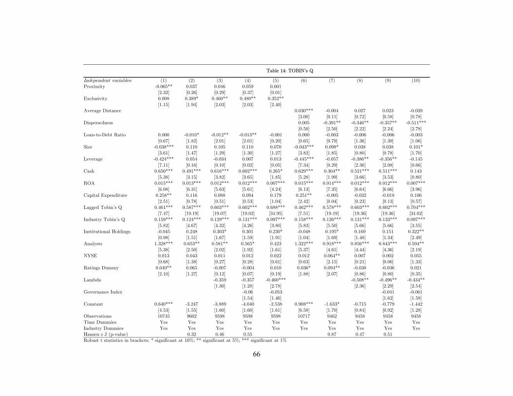
66

Table 14: TOBIN’s Q

Independent variables: (1) (2) (3) (4) (5) (6) (7) (8) (9) (10) Proximity -0.065** 0.037 0.046 0.059 0.001 [2.32] [0.26] [0.29] [0.37] [0.01] Exclusivity 0.008 0.389* 0.460** 0.480** 0.352** [1.15] [1.94] [2.03] [2.03] [2.40] Average Distance 0.030*** -0.004 0.027 0.023 -0.039 [3.00] [0.11] [0.72] [0.58] [0.78] Dispersedness 0.005 -0.391** -0.346** -0.357** -0.511*** [0.50] [2.50] [2.22] [2.24] [2.78] Loan-to-Debt Ratio 0.000 -0.010* -0.012** -0.013** -0.001 0.000 -0.003 -0.006 -0.006 -0.003 [0.67] [1.82] [2.01] [2.01] [0.20] [0.65] [0.79] [1.36] [1.39] [1.06] Size -0.038*** 0.110 0.105 0.110 0.070 -0.043*** 0.098* 0.038 0.038 0.101* [3.61] [1.47] [1.29] [1.30] [1.27] [3.82] [1.85] [0.80] [0.78] [1.70] Leverage -0.424*** 0.054 -0.034 0.007 0.013 -0.445*** -0.057 -0.386** -0.356** -0.145 [7.11] [0.16] [0.10] [0.02] [0.05] [7.34] [0.29] [2.36] [2.08] [0.66] Cash 0.650*** 0.491*** 0.616*** 0.602*** 0.265* 0.629*** 0.304** 0.521*** 0.511*** 0.143 [5.38] [3.15] [3.82] [3.65] [1.85] [5.28] [1.99] [3.66] [3.53] [0.80] ROA 0.015*** 0.013*** 0.012*** 0.012*** 0.007*** 0.015*** 0.014*** 0.012*** 0.012*** 0.007*** [6.08] [6.31] [5.63] [5.61] [4.24] [6.13] [7.35] [6.64] [6.66] [3.96] Capital Expenditure 0.258** 0.116 0.088 0.094 0.179 0.251** -0.005 -0.032 -0.018 0.106 [2.51] [0.78] [0.51] [0.53] [1.04] [2.42] [0.04] [0.23] [0.13] [0.57] Lagged Tobin’s Q 0.461*** 0.587*** 0.603*** 0.602*** 0.688*** 0.462*** 0.578*** 0.603*** 0.602*** 0.704*** [7.47] [19.19] [19.07] [19.02] [34.95] [7.51] [19.19] [19.36] [19.36] [34.02] Industry Tobin’s Q 0.159*** 0.124*** 0.129*** 0.131*** 0.097*** 0.158*** 0.126*** 0.131*** 0.133*** 0.097*** [5.82] [4.67] [4.32] [4.26] [3.80] [5.83] [5.50] [5.66] [5.66] [3.55] Institutional Holdings -0.045 0.248 0.303* 0.301 0.230* -0.048 0.195* 0.169 0.151 0.322** [0.98] [1.51] [1.67] [1.59] [1.91] [1.04] [1.69] [1.48] [1.34] [2.49] Analysts 1.328*** 0.653** 0.581** 0.565* 0.423 1.322*** 0.918*** 0.856*** 0.843*** 0.594** [5.38] [2.50] [2.02] [1.92] [1.61] [5.37] [4.61] [4.44] [4.36] [2.19] NYSE 0.013 0.043 0.011 0.012 0.022 0.012 0.064** 0.007 0.002 0.055 [0.68] [1.38] [0.27] [0.28] [0.61] [0.63] [2.15] [0.21] [0.06] [1.33] Ratings Dummy 0.040** 0.065 -0.007 -0.004 0.010 0.036* 0.094** -0.038 -0.036 0.021 [2.10] [1.27] [0.12] [0.07] [0.19] [1.88] [2.07] [0.86] [0.80] [0.35] Lambda -0.359 -0.357 -0.460*** -0.508** -0.496** -0.434** [1.30] [1.28] [2.78] [2.36] [2.29] [2.54] Governance Index -0.06 -0.053 -0.041 -0.061 [1.54] [1.46] [1.62] [1.58] Constant 0.640*** -3.247 -3.889 -4.040 -2.538 0.908*** -1.633* -0.715 -0.779 -1.442 [4.53] [1.55] [1.60] [1.60] [1.61] [6.58] [1.70] [0.84] [0.92] [1.28] Observations 10745 9602 9598 9598 9598 10717 9462 9458 9458 9458 Time Dummies Yes Yes Yes Yes Yes Yes Yes Yes Yes Yes Industry Dummies Yes Yes Yes Yes Yes Yes Yes Yes Yes Yes Hansen's J (p-value) 0.32 0.46 0.55 0.87 0.47 0.51 Robust t statistics in brackets; * significant at 10%; ** significant at 5%; *** significant at 1%

67

Table 15

Impact of the lending relationship on the firm’s stock returns This table exhibits abnormal returns from trading strategies devised on the basis of the firms’ loan characteristics. The abnormal returns in all the following panels are calculated with respect to four factors: the Fama-French 3-factors as well as momentum factor.

Panel A presents returns using the Ibbotson Returns Across Time and Securities (RATS) estimation. Therefore, the returns in this panel are returns over the indicated holding period. The numbers in brackets at the head of each column represent months after the loan, over which these stocks are held. E.g., [1, 6] would represent the 6-month period immediately after the month in which the loan started. Hi indicates the return on a portfolio consisting of firms whose loan-characteristic (proximity, or exclusivity, or average distance, or dispersedness) is above median in a given month, and Lo indicates the return on a portfolio consisting of firms whose loan-characteristic is either equal to or below median in that month.

Panels B and C present returns using a calendar-time portfolio strategy; Panel B shows returns of an equally-weighted portfolio and Panel C those of a value-weighted portfolio.

I.e., the column under the heading [1, 6] shows returns of a portfolio consisting of all stocks that started a loan within the past 6 months. Therefore, the returns in this panel are returns per month over the indicated period (i.e., the returns under [1, 6] are monthly returns for a period of 6 months immediately after the month in which the loan started.) Hi indicates the return on a portfolio consisting of firms whose loan-characteristic (proximity, or exclusivity, or average distance, or dispersedness) is above median in a given month, and Lo indicates the return on a portfolio consisting of firms whose loan-characteristic is either equal to or below median in that month. Hi — Lo represents a trading strategy where we go long in the Hi portfolio and short the Lo portfolio.

Panel A: Returns Across Time and Securities (RATS)

Months: [1, 1] [1, 3] [1, 6] [1, 12] Hi Lo Hi Lo Hi Lo Hi Lo Proximity 0.47% 0.02% 0.36% 0.02% -0.24% 0.37% 0.07% 1.27%* [1.44] [0.11] [0.65] [0.07] [-0.31] [0.79] [0.06] [1.90] Exclusivity 0.65%*** -0.38%* 0.84%** -0.63%* 2.17%*** -1.64%*** 4.37%*** -2.27%*** [2.63] [-1.92] [2.01] [-1.78] [3.45] [-3.23] [4.79] [-3.06] Average Distance -0.05% 0.33% -0.17% 0.39% 0.21% 0.28% 1.56%* 0.41% [-0.21] [1.50] [-0.44] [1.02] [0.36] [0.49] [1.89] [0.49] Dispersedness -0.32% 0.50%** -0.51% 0.61% -1.71%*** 1.89%*** -2.12%*** 3.62%*** [-1.50] [2.15] [-1.39] [1.54] [-3.25] [3.17] [-2.76] [4.18]

t-statistics are reported in brackets * significant at 10%; ** significant at 5%; *** significant at 1%

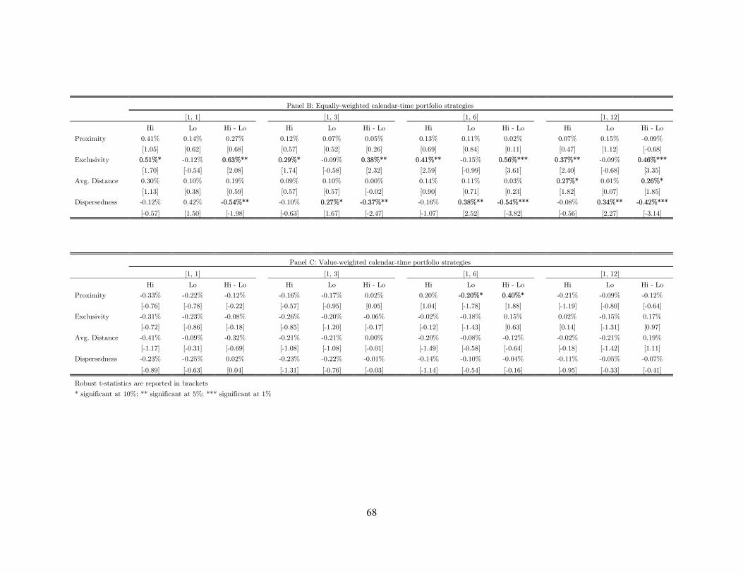
68

Panel B: Equally-weighted calendar-time portfolio strategies

[1, 1] [1, 3] [1, 6] [1, 12]

Hi Lo Hi - Lo Hi Lo Hi - Lo Hi Lo Hi - Lo Hi Lo Hi - Lo

Proximity 0.41% 0.14% 0.27% 0.12% 0.07% 0.05% 0.13% 0.11% 0.02% 0.07% 0.15% -0.09%

[1.05] [0.62] [0.68] [0.57] [0.52] [0.26] [0.69] [0.84] [0.11] [0.47] [1.12] [-0.68]

Exclusivity 0.51%* -0.12% 0.63%** 0.29%* -0.09% 0.38%** 0.41%** -0.15% 0.56%*** 0.37%** -0.09% 0.46%***

[1.70] [-0.54] [2.08] [1.74] [-0.58] [2.32] [2.59] [-0.99] [3.61] [2.40] [-0.68] [3.35]

Avg. Distance 0.30% 0.10% 0.19% 0.09% 0.10% 0.00% 0.14% 0.11% 0.03% 0.27%* 0.01% 0.26%*

[1.13] [0.38] [0.59] [0.57] [0.57] [-0.02] [0.90] [0.71] [0.23] [1.82] [0.07] [1.85]

Dispersedness -0.12% 0.42% -0.54%** -0.10% 0.27%* -0.37%** -0.16% 0.38%** -0.54%*** -0.08% 0.34%** -0.42%***

[-0.57] [1.50] [-1.98] [-0.63] [1.67] [-2.47] [-1.07] [2.52] [-3.82] [-0.56] [2.27] [-3.14]

Panel C: Value-weighted calendar-time portfolio strategies

[1, 1] [1, 3] [1, 6] [1, 12]

Hi Lo Hi - Lo Hi Lo Hi - Lo Hi Lo Hi - Lo Hi Lo Hi - Lo

Proximity -0.33% -0.22% -0.12% -0.16% -0.17% 0.02% 0.20% -0.20%* 0.40%* -0.21% -0.09% -0.12%

[-0.76] [-0.78] [-0.22] [-0.57] [-0.95] [0.05] [1.04] [-1.78] [1.88] [-1.19] [-0.80] [-0.64]

Exclusivity -0.31% -0.23% -0.08% -0.26% -0.20% -0.06% -0.02% -0.18% 0.15% 0.02% -0.15% 0.17%

[-0.72] [-0.86] [-0.18] [-0.85] [-1.20] [-0.17] [-0.12] [-1.43] [0.63] [0.14] [-1.31] [0.97]

Avg. Distance -0.41% -0.09% -0.32% -0.21% -0.21% 0.00% -0.20% -0.08% -0.12% -0.02% -0.21% 0.19%

[-1.17] [-0.31] [-0.69] [-1.08] [-1.08] [-0.01] [-1.49] [-0.58] [-0.64] [-0.18] [-1.42] [1.11]

Dispersedness -0.23% -0.25% 0.02% -0.23% -0.22% -0.01% -0.14% -0.10% -0.04% -0.11% -0.05% -0.07%

[-0.89] [-0.63] [0.04] [-1.31] [-0.76] [-0.03] [-1.14] [-0.54] [-0.16] [-0.95] [-0.33] [-0.41]

Robust t-statistics are reported in brackets

* significant at 10%; ** significant at 5%; *** significant at 1%