The CXTFIT Code for Estimating Transport

Parameters from Laboratory or Field

Tracer Experiments

Version 2.0

N. Toride, F. J. Leij, and M. Th. van Genuchten

Research Report No. 137

August 1995

U. S. SALINITY LABORATORY

AGRICULTURAL RESEARCH SERVICE

U. S. DEPARTMENT OF AGRICULTURE

RIVERSIDE, CALIFORNIA

DISCLAIMER

This report documents version 2.0 of CXTFIT, a computer program for estimating solute

transport parameters from observed concentrations (the inverse problem) or for predicting solute

concentrations (the direct problem) using the convection-dispersion equation as the transport model.

CXTFIT 2.0 is a public domain code, and as such may be used and copied freely. The code has been

verified against a large number of test cases. However, no warranty is given that the program is

completely error-free. If you do encounter problems with the code, find errors, or have suggestions

for improvement, please contact one of the authors’ at

U. S. Salinity LaboratoryUSDA, ARS450 West Big Springs RoadRiverside, CA 92507-46 17

Phone (909) 369-4850Fax (909) 342-4964e-mail titan@citrus.ucr.edu

‘The senior author may be reached at: Dept. of Agricultural Sciences, Saga Univ., Saga 840,Japan. Phone: +81-952-24-5191; Fax: +81-952-22-6274; E-mail: nobuo@cc.saga-u.ac.jp.

. . .111

ABSTRACT

N. Toride, F. J. Leij, and M. Th. van Genuchten. The CXTFIT Code for Estimating Transport

Parameters from Laboratory or Field Tracer Experiments, Version 2.0, Research Report No. 137,

U. S. Salinity Laboratory, USDA, ARS, Riverside, CA.

Successful predictions of the fate and transport of solutes in the subsurface hinges on the availability

of accurate transport parameters. We modified and updated the CXTFIT code of Parker and van

Genuchten [1984b] for estimating solute transport parameters using a nonlinear least-squares

parameter optimization method. The program may be used to solve the inverse problem by fitting

mathematical solutions of theoretical transport models, based upon the convection-dispersion

equation (CDE), to experimental results. This approach allows parameters in the transport models

to be quantified. The program may also be used to solve the direct or forward problem to determine

the concentration as a function of time and/or position. Three different one-dimensional transport

models are included: (i) the conventional CDE; (ii) the chemical and physical nonequilibrium CDE;

and (iii) a stochastic stream tube model based upon the local-scale CDE with equilibrium or

nonequilibrium adsorption. The two independent stochastic parameters in the stream-tube model are

the pore-water velocity, v, and either the dispersion coefficient, D, the distribution coefficient, Kd, or

the nonequilibrium rate parameter, a. These pairs of stochastic parameters were described with a

bivariate lognormal probability density function (pdf). Examples are given on how transport

parameters may be determined from laboratory or field tracer experiments for several types of initial

and boundary conditions, as well as different zero-order production profiles. A detailed description

is provided of the computer program, including the subroutines used to evaluate the analytical

solutions for optimizing model parameters. Input and output files for all major problems are included

in this manual.

Keywords: Solute transport, parameter estimation, convection-dispersion equation, analytical

solutions, nonequilibrium transport, stochastic transport, stream tube model.

V

1. INTRODUCTION

The fate and movement of dissolved substances in soils and groundwater has generated

considerable interest out of concern for the quality of the subsurface environment. The behavior of

solutes over relatively long spatial and temporal scales has to be assessed with the help of theoretical

models since it is usually not feasible to carry out experimental studies over sufficiently long distances

and/or time periods. Mathematical models are often used to predict solute concentrations before

management strategies are implemented. Advances in software and hardware now permit the

simulation of subsurface transport using sophisticated mathematical models. Unfortunately, it is

generally diicult to obtain reliable values for transport parameters such as the pore-water velocity,

the retardation factor, the dispersion coefficient, and degradation or production parameters.

The program CXTFIT 2.0 may be used to estimate parameters in several models for transport

during steady one-dimensional flow by fitting the parameters to observed laboratory or field data

obtained from solute displacement experiments. The inverse problem is solved by minimizing an

objective function, which consists of the sum of the squared differences between observed and fitted

concentrations. The objective function is minimized using a nonlinear least-squares inversion method

according to Marquardt [1963]..In addition, CXTFIT 2.0 may also be used for the direct problem

to predict solute distributions versus time and/or space for specified model parameters.

CXTFIT 2.0 is an extension and update of an earlier version program published more than ten

years ago by Parker and van Genuchten [1984b].. The new CXTFIT, version 2.0, again uses the

convection-dispersion equation, but with a greater number of analytical solutions to various initial,

boundary, and production value problems. The nonequilibrium transport models now contains also

terms for zero-order production and first-order decay. Considerably more attention is being paid to

the use of stream tube models for simulating transport in heterogenous fields, thus reflecting the

growing popularity of stochastic approaches for modeling field-scale solute transport. A bivariate

lognormal probability density function is used to quantify stochastic flow and either stochastic

dispersion, adsorption, or nonequilibrium solute transfer. Solute concentrations across the field can

be in the resident mode or in two different types of flux-averaged modes.

This report serves to document the CXTFIT 2.0 computer program. Equilibrium transport

according to the convection-dispersion equation (CDE) is reviewed in Chapter 2. The mathematical

1

problem is first stated, and solutions for the initial value problem (IVP), the boundary value problem

(BVP), and the production value problem (PVP) are listed. The program may be used to estimate

the pore-water velocity (v), the dispersion coefficient (D), the retardation factor (R), the first-order

degradation coefficient (,u), and/or the zero-order production coefficient (r) from observed

concentration distributions versus time and/or distance. Nonequilibrium transport is discussed in

Chapter 3 in terms of alternative physical and chemical nonequilibrium models. Solutions of the

(bimodal) dimensionless nonequilibrium transport equation are presented for the same cases as for

equilibrium transport. In addition to v, D, R, p, and r, the coefficient of partitioning between the

equilibrium and nonequilibrium phases Cp, and the mass transfer coefficient (0) for transfer between

the two phases can now be fitted as well. Chapter 4 describes the stream tube model as a relatively

simple conceptualization of solute transport in heterogeneous fields. Transport in each stream tube

(the local scale) is described with the CDE as an initial or a boundary value problem. Pairs of

stochastic parameters, one always being v, are used in solutions of the CDE. Transport at the field

scale is subsequently modeled by averaging the local concentrations.

Chapter 5 provides details about the numerical evaluation of some of the analytical functions,

including the numerical integration procedures. This chapter also gives an outline of the parameter

estimation procedure. Chapter 6 serves as user’s guide for the program. This chapter lists all

available transport models and gives instructions on how to solve the inverse problem. All possible

variables in the input file are documented in terms of separate blocks. The blocks pertain to model

selection, solution of the inverse problem definition of transport parameters, stipulation of boundary,

initial, as well as production conditions, and specification of times and positions for which the direct

problem is to be solved. Examples of input and output files are also provided. The examples are

those given on the diskette accompanying this manual. Finally, Chapter 7 illustrates the use of

CXTFIT 2.0 for several forward and inverse problems.

2

use of flux-averaged or flowing concentrations in the mathematical model [Kreft and Zuber, 1978;

Parker and van Genuchten, 1984a]. Flux-averaged concentrations are defined as the ratio of the

solute and water fluxes; they occur, for example, if a solute breakthrough curve is determined from

effluent samples. The specification of the type of concentration is discussed in Chapter 7.

For transport according to the CDE, the flux-averaged concentration can be obtained from the

resident concentration using the transformation:

1 ac,c/ = c, - - -P az

(2.13)

where the subscriptfrefers to a flux-averaged concentration. Expressions for C,are easily derived

by substituting the solution for C, for a third-type inlet condition into (2.13). We may drop the

subscript of C if the difference between the two concentration modes is immaterial or if it is clear that

we refer to a resident concentration.

Superposition

Since the governing equations and the initial and boundary conditions are linear in C, the

superposition principle - as explained, for example, in Farlow [ 1982] -- may be used to express the

analytical solution as the sum of three independent subproblems involving a boundary value problem

(BVP), an initial value problem (IVP), and a production value problem (PVP). The overall solution

can then be written as

C(Z,T) = P(ZJ) + C ‘(ZJ) + CP(Z,7-) (2.14)

where the superscripts B, I and P denote the boundary, initial, and production value problems,

respectively. We first present the general solution to each subproblem, subsequently we give several

specific solutions.

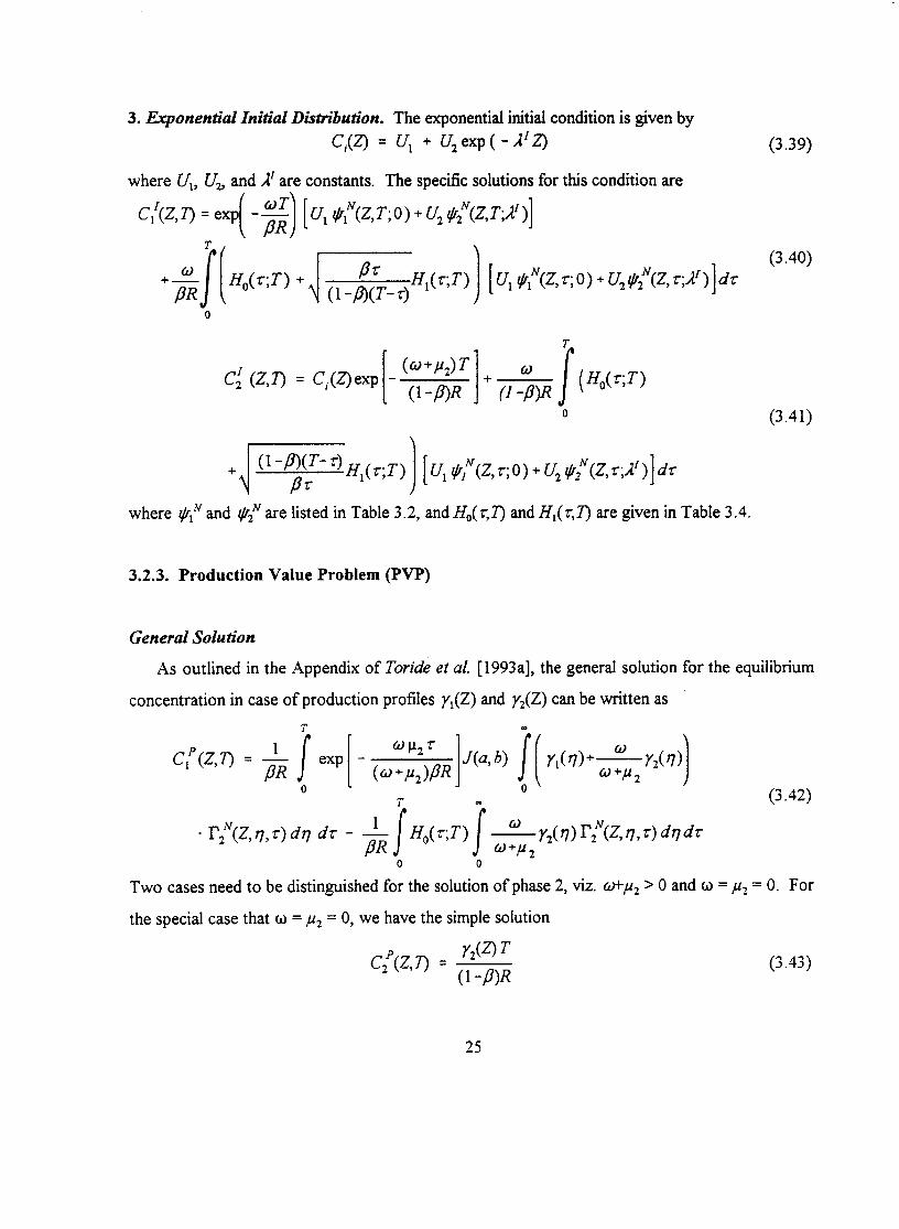
6

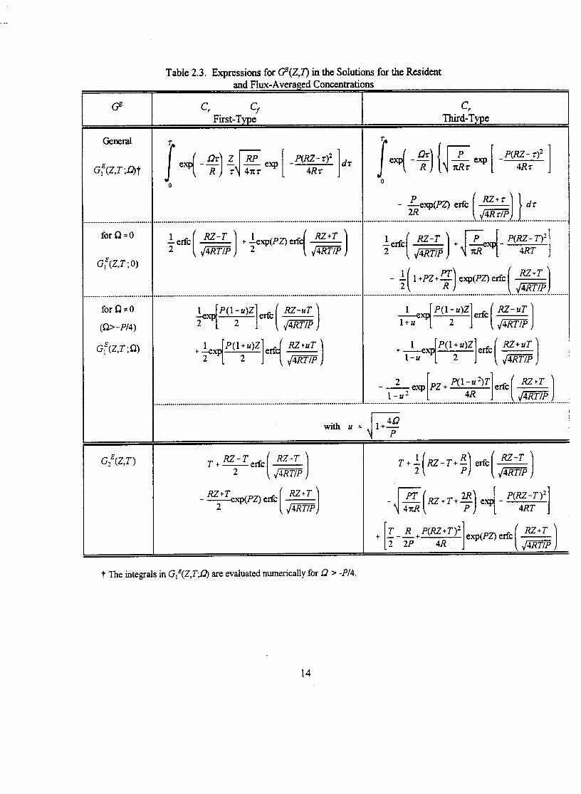
C p(ZT) = Y, G:CW lR (2.3 5)

where G,‘(Z,T) is given in Table 2.3.

2. Exponential Production Profile.

in a manner similar as for the IVP:

YE(z)where yI, y2, and ,I’ are constants.

T

Solute production can be expressed as an exponential function

= Yl+ Y*exP( -nPz)The solution is now given by

(2.36)

T

+GzE(Z,n + ;I&Z, t;Ap )dr

\ 0

(2.37)

where PIE and I&~ are given in Table 2.2, while GIE(Z,T,Q) and GzE(Z,T) are defined in Table 2.3.

12

at equilibrium, and the subscripts e and k refer to equilibrium and kinetic adsorption sites,

respectively. Equations (3.1) and (3.2) use the customary first-order rate expression for describing

kinetic adsorption on type-2 sites. The two-site adsorption model reduces to the one-site fully kinetic

adsorption model iff= 0 (only type-2 sites are present). The one-site model is used in Section 4.2

in the stream-tube formulation for field transport.

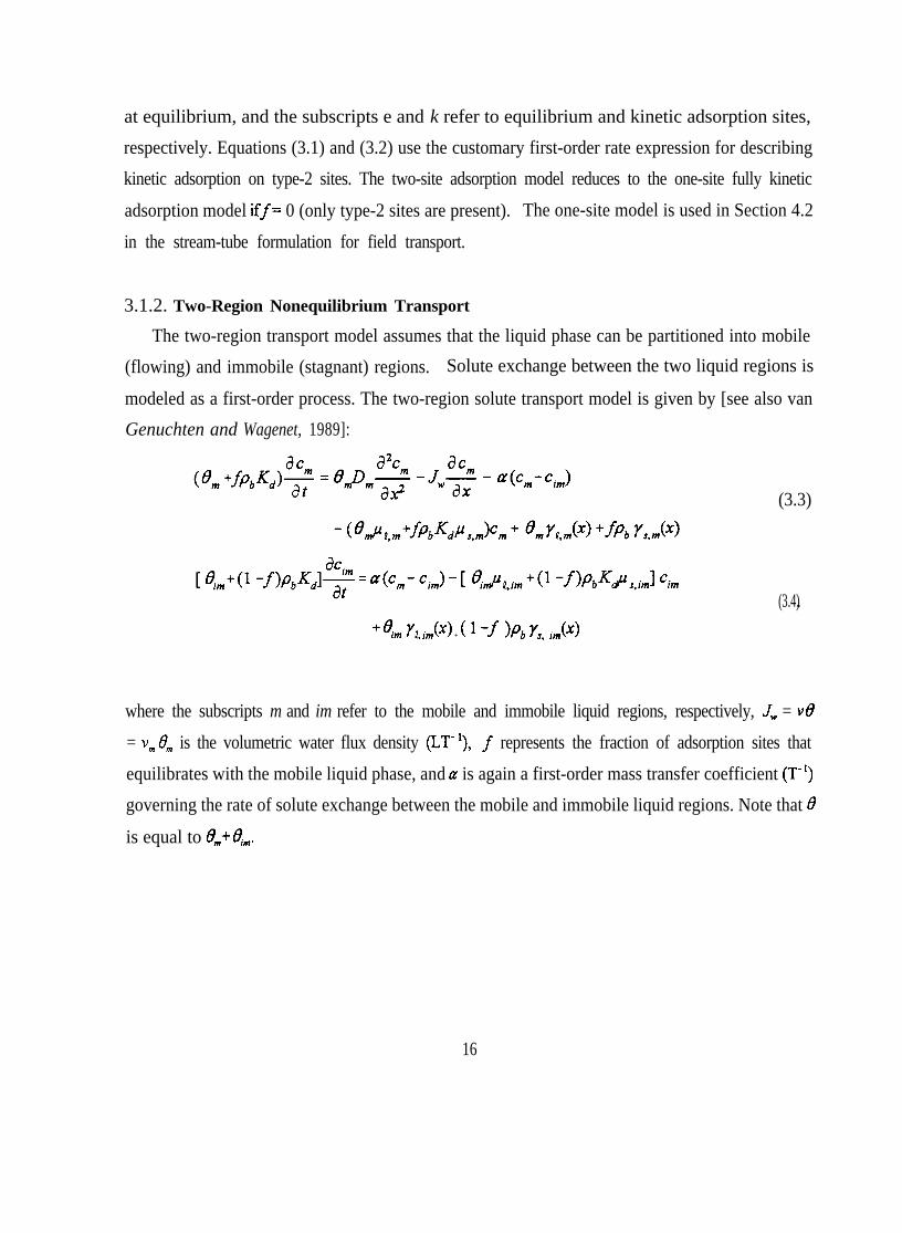
3.1.2. Two-Region Nonequilibrium Transport

The two-region transport model assumes that the liquid phase can be partitioned into mobile

(flowing) and immobile (stagnant) regions. Solute exchange between the two liquid regions is

modeled as a first-order process. The two-region solute transport model is given by [see also van

Genuchten and Wagenet, 1989]:

(3.3)

(3.4) .+ 8,, U$, jmCX> + ( ’ -f )Pb Us, jmCX)

where the subscripts m and im refer to the mobile and immobile liquid regions, respectively, J, = v0

= v, 8, is the volumetric water flux density (LT- ‘), f represents the fraction of adsorption sites that

equilibrates with the mobile liquid phase, and a is again a first-order mass transfer coefficient (T-r)

governing the rate of solute exchange between the mobile and immobile liquid regions. Note that 0

is equal to em+em.

16

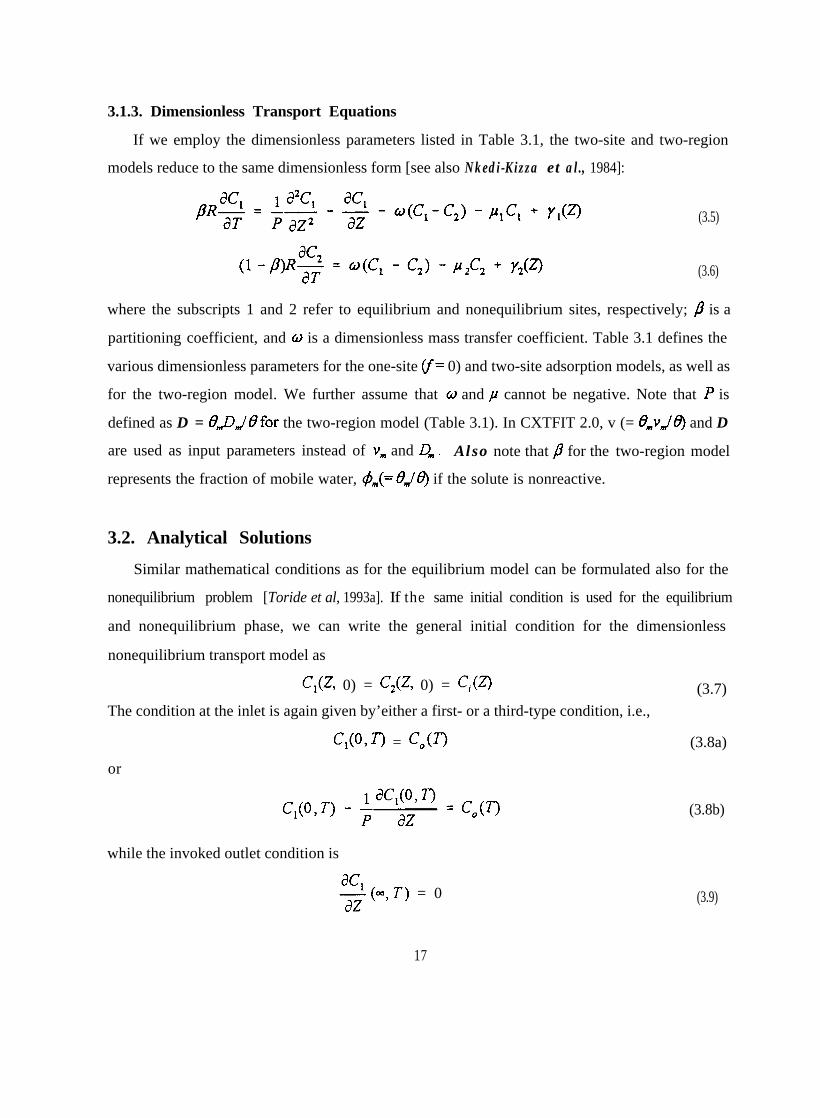
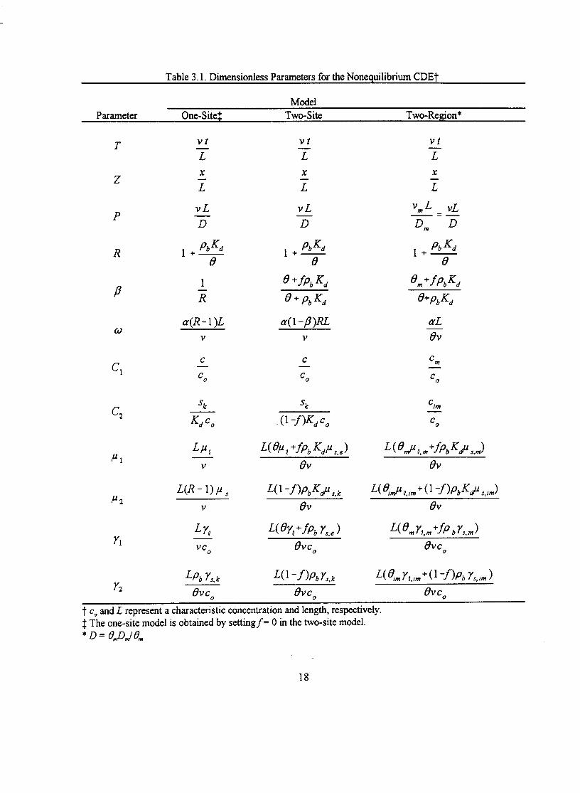
3.1.3. Dimensionless Transport Equations

If we employ the dimensionless parameters listed in Table 3.1, the two-site and two-region

models reduce to the same dimensionless form [see also Nkedi-Kizza et al., 1984]:

(3.5)

(3.6)

where the subscripts 1 and 2 refer to equilibrium and nonequilibrium sites, respectively; p is a

partitioning coefficient, and o is a dimensionless mass transfer coefficient. Table 3.1 defines the

various dimensionless parameters for the one-site cf= 0) and two-site adsorption models, as well as

for the two-region model. We further assume that o and ,U cannot be negative. Note that P is

defined as D = 8,&,,,/0for the two-region model (Table 3.1). In CXTFIT 2.0, v (= e,v,,,/@ and D

are used as input parameters instead of v, and 0,. Also note that p for the

represents the fraction of mobile water, #,(= 8J8) if the solute is nonreactive.

3.2. Analytical Solutions

two-region model

Similar mathematical conditions as for the equilibrium model can be formulated also for the

nonequilibrium problem [Toride et al, 1993a]. If the same initial condition is used for the equilibrium

and nonequilibrium phase, we can write the general initial condition for the dimensionless

nonequilibrium transport model as

C&Z, 0) = C,(Z 0) = C,(z> (3.7)

The condition at the inlet is again given by’either a first- or a third-type condition, i.e.,

C,(OJJ = C,(T) (3.8a)

or

while the invoked outlet condition is

2 (m, T) = 0

(3.8b)

(3.9)

17

3.2.1. Boundary Value Problem (BVP)

General solution

Concentrations as a result of an arbitrary input function, C,(T), can be expressed as

T

C,B(Z,T) =I

C&T- r) f(Z r)dr0

(3.13)

(3.14)

(3.15)

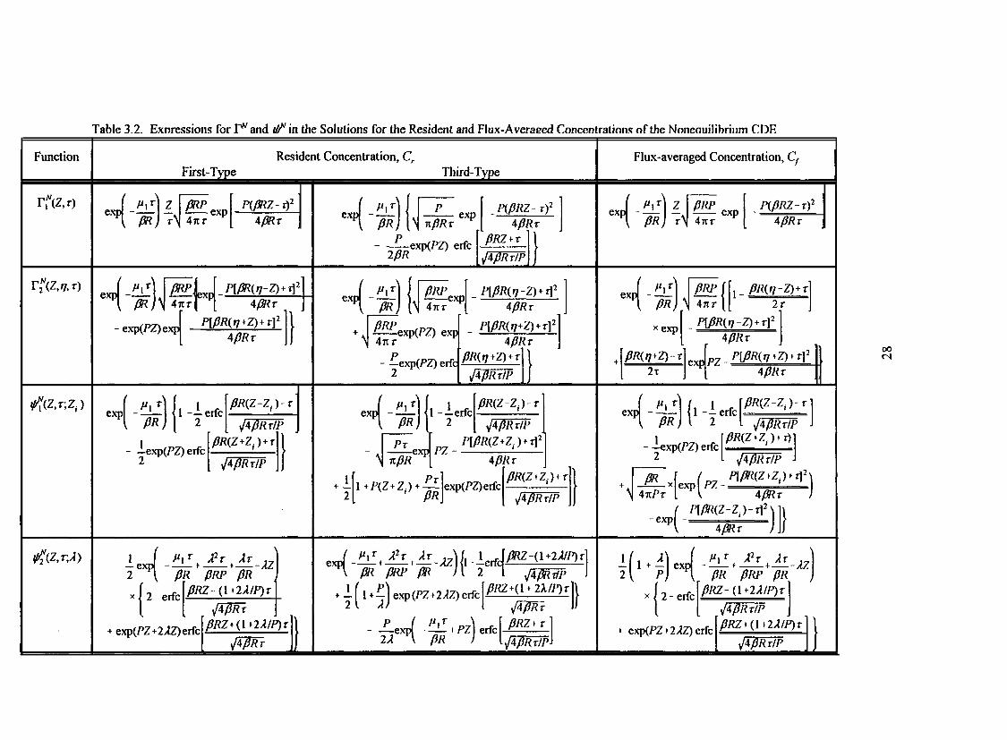
with I’,“(Z, r) given in Table 3.2 and where the superscript refers to the nonequilibrium solution.

Furthermore, H,(t,T) is given in Table 3.4 with I, as the modified Bessel function of order one.

Below we give specific solutions for cases where C,(T) in (3.8) is described by a Dirac delta, a

multiple pulse, and an exponential function.

Specific Solution

1. Dirac Delta Input Function. The inlet condition for a Dirac delta fimction is (cf. (2.16a)):

C,(T) = M-s S(O (3.16)

Substitution of (3.16) into the general solutions leads to the following specific solutions:

C,B(Z, Q = M,f(Z,O (3.17)

T

MS0CGQ = (l_*R I I';(Z,r) H,(r;T) dr

0

(3.18)

where the nonequilibrium travel time pdf, AZ, T), is given by (3.15) l?,“(Z, r) can be found in Table

3.2, and HO{ r,7) is given in Table 3.4 with I, as the modified Bessel function of order zero.

20

where G,“(Z,T;Q) is given in Table 3.3. CXTFIT always assumes that pi+o,~+/(wt,& r 0, which

is consistent with earlier assumptions that pi and pUt 2 0. Differentiating the solutions for a single step

input (i.e., A,(Z,I) and AiZ,T)) with respect to T yields the travel time pdf (cf. (3.17) and (3.18)) [De

Smedt and Wierenga, 1979].

3. Exponential Input Function. The exponential input function is given by

G,(T) =fi +fiexp(-+W (3.25)wherefi,fb and A’ are constants. As described by Leij et al. [1993], an approximate solution for this

exponential input can be derived by using the series expansion of the zero-order modified Bessel

function [9.6.12 of Abramowitz and Stegun, 1970]:

CF(Z,I) =f,A,(Z,T) +f,exp( -AE7)Gr Z,T;p,+o+ pRpqi

- - flRABP-q I

T

- ftev(-qT+‘:(Z&vI

Q,(t) dt0

-+(o-PRq)

(3.26)

with

and

,=Q= ia2 b o+Iu2

t (@+PL))PR ’ ’ = T-r = (1 -p)R

(3.27)

(3.28)

(3.29)

(3.30a,b)

The auxiliary functions A,(Z,T) and A,(Z,T) are given by (3.21) and (3.22), respectively. In analogy

to the equilibrium solution of the BVP for an exponential input (cf. (2.22)), the parameter u in

22

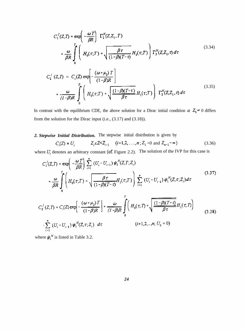
(3.34)

C,l (Z,lJ = Ci(Z)exp -(o+lu,) T

[ 1Cl-PP(3.35)

In contrast with the equilibrium CDE, the above solution for a Dirac initial condition at Z, = 0 differs

from the solution for the Dirac input (i.e., (3.17) and (3.18)).

2. Stepwise Initial Distribution. The stepwise initial distribution is given by

c,(Z, = ‘i Zi<Z<Zi+, (i=1,2, . . ..n ; Z, =0 and Z,,+i- w) (3.36)

where V, denotes an arbitrary constant (cf. Figure 2.2). The solution of the IVP for this case is

where hN is listed in Table 3.2.

24

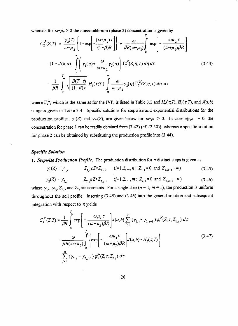
. fZ (Yz,j - Yz,j-1) PINC&r;Z~,j) (i= 1,2 ,...,n;j=l

Y~,~ = Y*,~ = 0)

where PI;” is listed in Table 3.2.

2. Exponential Production Profile. The depth-dependent production terms are given by:

Y&Z) = Yk;l + Yk,zexP( -0) (k=1,2) (3.49)

where Yk;l, Yk2, and Akp are constants. The concentrations are now given by

(3.50)

* Cl -J@Al [Y1,19&%0)+ yl,*qqZ,t; A;>]

+[ *exp[ - (@;;;?..J

* [Y, 1 ‘I’#, r, 0) + Y~,~ lcIz(Z t; &=jl

(3.51)

27

28

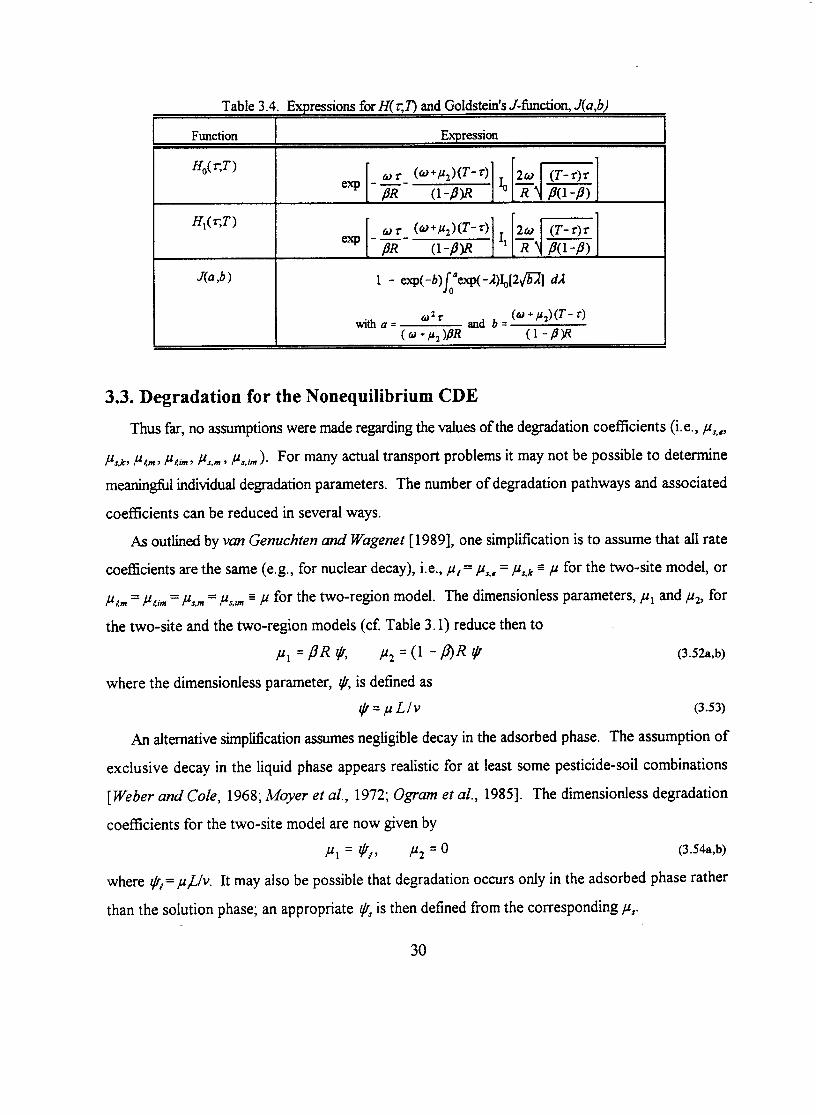
Table 3.5 summarizes the expressions for ,L+ and ,u2 in terms of @for the most general case as well

as for several limiting scenarios. We have furthermore assumed that the degradation coefficients for

decay in the liquid or adsorbed phase are the same for both regions in the two-region model when

degradation takes place exclusively in the liquid or adsorbed phase.

Table 3.5. Expressions for the Dimensionless Parameters p, and pL2 in (3.5) and (3.6)

Independent degradations

rates in liquid and

adsorbed phases

One-site model

P’1 = PJ

p2 = CR - 1W.s

Identical degradation in PI = P P, =PRP ~1 =PR@

liquid and adsorbed phases pz = (R - 1W P2=W-#W P* =(l-p)RP

No degradation in the

adsorbed phase

No degradation in the

liquid phase

31

4. STREAM TUBE MODEL FOR FIELD-SCALE TRANSPORT

4.1. Introduction

Traditional deterministic approaches based upon the convection-dispersion equation (CDE) for

chemical transport and the Richards equation for water flow work relatively well for homogeneous

soils and packed laboratory soil columns. However, most field soils are far from homogeneous,

resulting in sometimes highly nonuniform flow and transport processes. Experimental investigations

at the field scale have demonstrated the effects of heterogeneity on solute transport [e.g., Biggar and

Nielsen, 1976; Sudicky, 1986]. A variety of stochastic modeling approaches have been employed to

describe nonreactive solute transport in a heterogeneous flow field [e.g., Dagan, 1984; Sposito and

Barry, 1987]. Recently, stochastic methods have also been used to study solute transport subject to

equilibrium [Kabala and Sposito, 1991] or nonequilibrium adsorption [e.g., Dagan and Cvetkovic,

1993; Bel l in et al., 1993]. In these investigations, a transport equation in terms of a mean solute

concentration across the field is formulated using the covariance functions of local-scale transport

parameters. Unfortunately, it is usually not possible to determine a reliable statistical distribution for

each parameter.

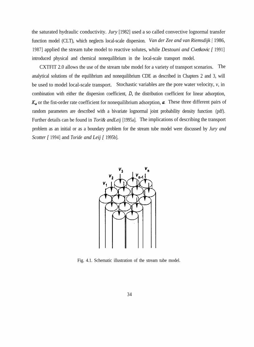
In a simplified approach to stochastic modeling, the field may be viewed as a series of independent

vertical soil columns (cf. Figure 4.1). These columns are generally referred to as “stream tubes”

[Dagan, 1993; Jury and Roth, 1990]. Local-scale transport in each stream tube is described

deterministically assuming a convective or convective-dispersive model. Transport at the field scale

may be modeled by viewing selected parameters in the convective or convective-dispersive model for

each tube as realizations of a stochastic process. The mean solute concentration for an entire field

is given by the ensemble average of the local concentrations in all stream tubes. At the field scale,

the one-dimensional CDE (perfect mixing perpendicular to the flow direction) and the stream tube

model (no mixing between tubes) constitute the limiting cases for solute transport [Jury and FZiihZer,

1992].

There are several ways in which the stream tube model has been used to quantify solute transport

in heterogeneous soils. Dagan and Bresler [ 1979] and Bresler and Dagan [ 1979] described the

downward movement of nonreactive solutes at the field scale assuming a lognormal distribution for

33

the saturated hydraulic conductivity. Jury [1982] used a so called convective lognormal transfer

function model (CLT), which neglects local-scale dispersion. Van der Zee and van Riemsdijk [ 1986,

1987] applied the stream tube model to reactive solutes, while Destouni and Cvetkovic [ 1991]

introduced physical and chemical nonequilibrium in the local-scale transport model.

CXTFIT 2.0 allows the use of the stream tube model for a variety of transport scenarios. The

analytical solutions of the equilibrium and nonequilibrium CDE as described in Chapters 2 and 3, will

be used to model local-scale transport. Stochastic variables are the pore water velocity, v, in

combination with either the dispersion coefficient, D, the distribution coefficient for linear adsorption,

K& or the fist-order rate coefficient for nonequilibrium adsorption, g. These three different pairs of

random parameters are described with a bivariate lognormal joint probability density function (pdf).

Further details can be found in Tori& andLeij [1995a].. The implications of describing the transport

problem as an initial or as a boundary problem for the stream tube model were discussed by Jury and

Scotter [ 1994] and Toride and Leij [ 1995b].

Fig. 4.1. Schematic illustration of the stream tube model.

34

The solution of the local-scale transport equation depends exclusively on random transport

parameters such as v, D, and Kd, once the independent variables t and x have been specified. For

example, Figure 4.2a shows the solution, c, for the equilibrium CDE as a function of v and Kd at t

= 5 d for a 2-d pulse input at x = 100 cm assuming D = 20 cm* d’ and p,/8= 4 g cm“ (cf. (2.20)).

The concentration is normalized using the input concentration, c,. As Kd increases, the solute moves

slower because of increased adsorption; a higher v is required for the solute to reach x = 100 cm at

t=5d.

4.3 Field-Scale Transport

4.3.1. Bivariate Lognormal Distribution

The pairs of stochastic parameters in the local-scale model for transport in each stream tube are

obtained from a bivariate lognormal joint probability density function (pdf). Because of their

relatively low coefficient of variation, CV, the same values for 8 and pb are used for each stream tube.

The joint pdfs of v, in conjunction with either D, &, or 4 are written asflv,D),Av,&), andflv, a),

respectively. The general bivariate lognormal joint pdf is defined as [Spiegel, 1992; p. 118]:

f(v, 7) =1

/-

exp -r,2 -2&Y, Y7 + Y;

2xu”uqv 17 1 -pt, ! 2 (1 -P$ I

with

y = W) -P, y = WI) -PI.)Y

a” ’ rl%

(4.8)

(4.9a,b)

where q denotes D, Kd, or a (i.e., the second random parameter in addition to v), ,u and aare the

mean and standard deviation of the log-transformed variable, and ,uV,, is the correlation coefficient

between Y, and Y7.

36

Fig. 4.2. Predicted resident concentrations according to the stream tube model:(a) local-scale c, as a function of v and Kd at x = 100 cm and t = 5 d;

(b) a bivariate lognormal pdf for pVm = -0.5; and(c) expected c, at x = 100 cm and t = 5 d.

37

The ensemble averages of v and TJ are given by [Aitcheson and Brown, 1963; p. S]:

<v>=exp r.+Lgt ,( 1

1 2

2<q;=exp p +_orl

( )Q 2(4.1la,b)

with the coefficient of variation CV expressed as

CV(v) = \l*, CV(?)) =&gqT (4.12a,b)

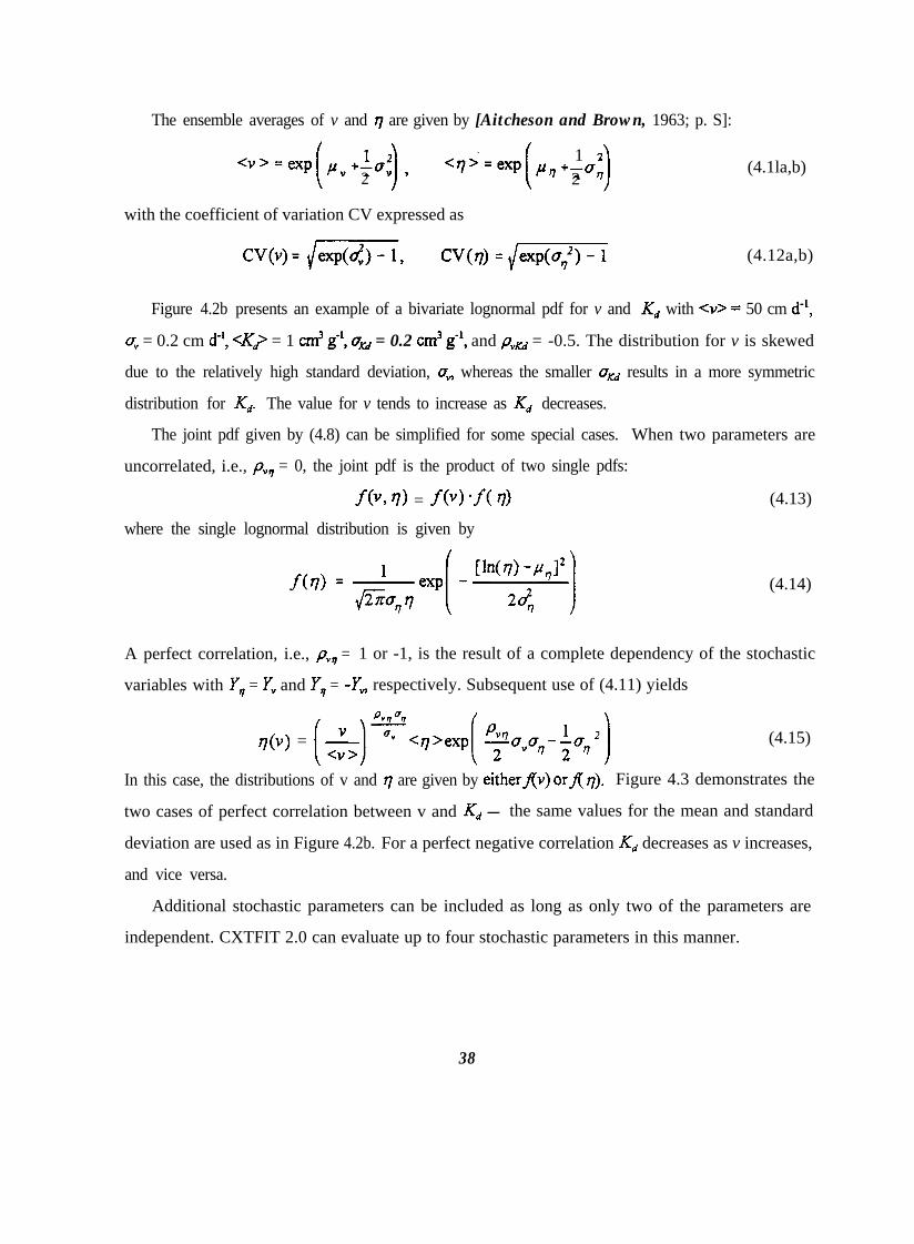
Figure 4.2b presents an example of a bivariate lognormal pdf for v and Kd with <I.+ = 50 cm d“,

a, = 0.2 cm d-l, <IQ = 1 cm3 g*‘, a, = 0.2 cm3 g-‘, and pyKd = -0.5. The distribution for v is skewed

due to the relatively high standard deviation, a,,, whereas the smaller a,, results in a more symmetric

distribution for Kk The value for v tends to increase as Kd decreases.

The joint pdf given by (4.8) can be simplified for some special cases. When two parameters are

uncorrelated, i.e., p,,,, = 0, the joint pdf is the product of two single pdfs:

f(v, rl) = f(v) .f( rl) (4.13)

where the single lognormal distribution is given by

(4.14)

A perfect correlation, i.e., py,, = 1 or -1, is the result of a complete dependency of the stochastic

variables with Y7 = Y, and Y7 = -Y, respectively. Subsequent use of (4.11) yields

q(v) = ($)?<q>exp( $bvuq-+uq2) (4.15)

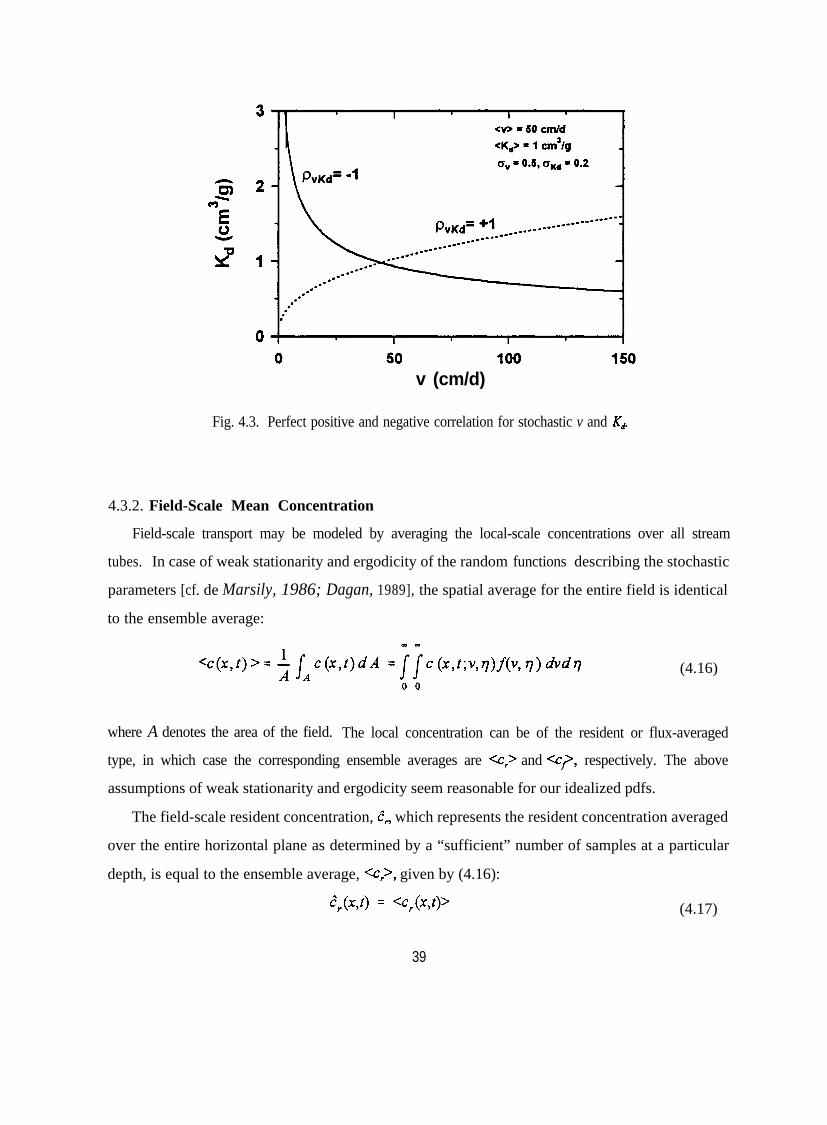
In this case, the distributions of v and TJ are given by eitherflv) orf( q). Figure 4.3 demonstrates the

two cases of perfect correlation between v and Kd - the same values for the mean and standard

deviation are used as in Figure 4.2b. For a perfect negative correlation Kd decreases as v increases,

and vice versa.

Additional stochastic parameters can be included as long as only two of the parameters are

independent. CXTFIT 2.0 can evaluate up to four stochastic parameters in this manner.

38

v (cm/d)

Fig. 4.3. Perfect positive and negative correlation for stochastic v and K+

4.3.2. Field-Scale Mean Concentration

Field-scale transport may be modeled by averaging the local-scale concentrations over all stream

tubes. In case of weak stationarity and ergodicity of the random functions describing the stochastic

parameters [cf. de Marsily, 1986; Dagan, 1989], the spatial average for the entire field is identical

to the ensemble average:

COOOD

<c(x,t)> = 1 IA Ac(x,t)dA = II c (x,f;w)f(v, 17) bdrl

0 0

(4.16)

where A denotes the area of the field. The local concentration can be of the resident or flux-averaged

type, in which case the corresponding ensemble averages are <c, and -7, respectively. The above

assumptions of weak stationarity and ergodicity seem reasonable for our idealized pdfs.

The field-scale resident concentration, c^, which represents the resident concentration averaged

over the entire horizontal plane as determined by a “sufficient” number of samples at a particular

depth, is equal to the ensemble average, <c,>, given by (4.16):

c^,(x,t) = <cJx,t)> (4.17)

39

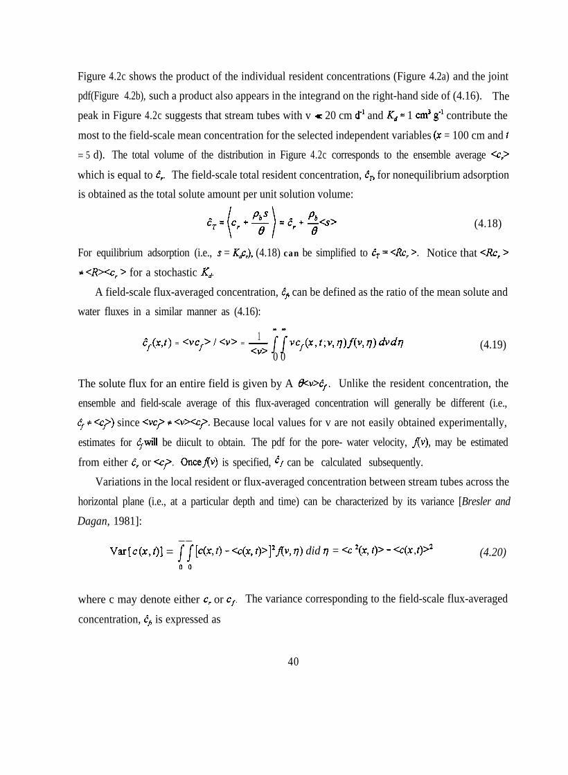
Figure 4.2c shows the product of the individual resident concentrations (Figure 4.2a) and the joint

pdf(Figure 4.2b), such a product also appears in the integrand on the right-hand side of (4.16). The

peak in Figure 4.2c suggests that stream tubes with v a 20 cm d“ and Kd = 1 cm3 g-r contribute the

most to the field-scale mean concentration for the selected independent variables (x = 100 cm and t

= 5 d). The total volume of the distribution in Figure 4.2c corresponds to the ensemble average <c,

which is equal to C$ The field-scale total resident concentration, Clr, for nonequilibrium adsorption

is obtained as the total solute amount per unit solution volume:

= cr f (4.18)

For equilibrium adsorption (i.e., s = K&J, (4.18) can be simplified to clr = CRC, >. Notice that CRC, >

# <R><c, > for a stochastic K,+

A field-scale flux-averaged concentration, $ can be defined as the ratio of the mean solute and

water fluxes in a similar manner as (4.16):-ooD

1qx,t> = <vc,> / <v> = -

<V> IIVCf(x, t;v, W(V, 7) hdrl (4.19)

0 0

The solute flux for an entire field is given by A &WI. Unlike the resident concentration, the

ensemble and field-scale average of this flux-averaged concentration will generally be different (i.e.,

$ + <c)) since <vc) + <v><cF. Because local values for v are not easily obtained experimentally,

estimates for Gwill be diicult to obtain. The pdf for the pore- water velocity, Av), may be estimated

from either c^, or <c). OncefTv) is specified, Ef can be calculated subsequently.

Variations in the local resident or flux-averaged concentration between stream tubes across the

horizontal plane (i.e., at a particular depth and time) can be characterized by its variance [Bresler and

Dagan, 1981]: __

: = /p4~>0 - <c(x, t)>12Av, 7) did 17 = <c ‘(x, t)> - <c(x,t>>20 0

(4.20)

where c may denote either c, or cr. The variance corresponding to the field-scale flux-averaged

concentration, I?+ is expressed as

40

Pulse-Type Application

Following Parker and van Genuchten [ 1984b], we study the BVP involving a finite pulse input

for the case of either a constant or variable application time for each tube. Consider a pulse-type

solute application of concentrationf, and application time tz (cf. Figure 2.1). If t2 is constant for all

stream tubes, the amount of solute in each tube, mB =fit2v, is directly proportional to the random

velocity, v. The field-averaged mean, -2, is given byf&<v>. However, the same amount of mass,

mB , can be delivered to each tube by setting the application time inversely proportional to the

velocity, i.e., t2 = mJV;v). This scenario, where both v and 22 are random, may occur when solid

chemicals are added uniformly across the field and leached subsequently by continuously applying

solute-free water. The input concentration, fi, is regarded as approximately constant since this

concentration may be governed by the solubility of the chemical. Figure 4.6 schematically illustrates

the solute distribution between tubes for a pulse input of constant and variable duration.

Figure 4.7 presents field-scale resident concentrations (8,) versus depth at t = 3 d as a result of

a pulse-type solute application with a constant (t2 = 1 d) and variable (<t2> = 1 d) solute application

time. The same amount of solute is applied to the entire field. The transport parameters for this

example are the same as those used for Figure 4.5. Again, more solute remains near the surface for

the constant mass injection. Since the amount of solute in stream tubes with a higher v is larger for

the constant duration scenario, solute moves down faster in this case compared to the case of a

variable solute application time.

We emphasize that the previous examples involving Dirac- and pulse-type applications are

somewhat hypothetical since the stream tube model does not permit mixing between stream tubes.

Redistribution between stream tubes is likely to establish an intermediate situation where the mass

in each stream tube is not constant, but where differences between tubes are also not as large as for

the constant duration case because of horizontal mixing. Some horizontal mixing will likely also

occur at the surface.

44

Constant duration Variable duratlon

Fig. 4.6. Illustration of the solute distribution in stream tubesafter a pulse application of constant and variable duration.

OS510.4 -I

t=3d 4Variable duration

0 100 200 300 400

x (cm)

Fig. 4.7. Field-scale resident concentrations (6,) versus depth as a resuitof a pulse-type solute application of constant and variable duration.

45

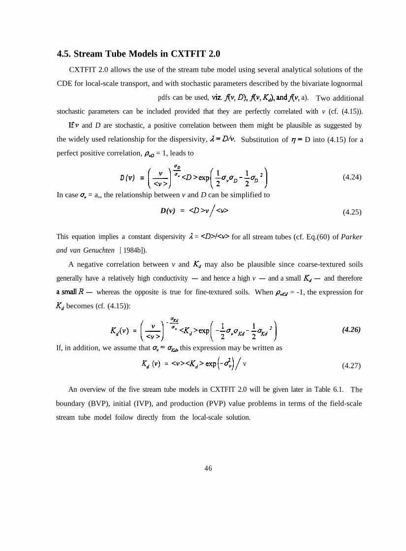
4.5. Stream Tube Models in CXTFIT 2.0

CXTFIT 2.0 allows the use of the stream tube model using several analytical solutions of the

CDE for local-scale transport, and with stochastic parameters described by the bivariate lognormal

pdf given by (4.9).Three different pdfs can be used, viz. j(v, D), Av, KJ, andf(v, a). Two additional

stochastic parameters can be included provided that they are perfectly correlated with v (cf. (4.15)).

Ifv and D are stochastic, a positive correlation between them might be plausible as suggested by

the widely used relationship for the dispersivity, /I = D/v. Substitution of q = D into (4.15) for a

perfect positive correlation, pVO = 1, leads to

D(v) = (5) ?<D>exp( igV*D-$, ‘)

In case a,, = a,, the relationship between v and D can be simplified to

D(v) = <D>v/

<v>

(4.24)

(4.25)

This equation implies a constant dispersivity /I = <D>/<v> for all stream tubes (cf. Eq.(60) of Parker

and van Genuchten [ 1984b]).

A negative correlation between v and Kd may also be plausible since coarse-textured soils

generally have a relatively high conductivity - and hence a high v - and a small Kd - and therefore

asmallR - whereas the opposite is true for fine-textured soils. When pyKd = -1, the expression for

Kd becomes (cf. (4.15)):

(4.26)

If, in addition, we assume that a, = a,, this expression may be written as

Kd w = <v><K,>exp -d’,( )/ v (4.27)

An overview of the five stream tube models in CXTFIT 2.0 will be given later in Table 6.1. The

boundary (BVP), initial (IVP), and production (PVP) value problems in terms of the field-scale

stream tube model foilow directly from the local-scale solution.

46

5. NUMERICAL EVALUATION

The FORTRAN program CXTFIT 2.0 was written to evaluate the one-dimensional analytical

solutions that were discussed in Chapters 2 through 4. In this chapter we will provide background

information on numerical procedures followed to solve the direct and inverse problems. First, the

main program units of CXTFIT 2.0 are briefly reviewed. The numerical evaluation of the integrals

and various special functions in the analytical solutions are discussed subsequently. The previous

version of CXTFIT published by Parker and van Genuchten [1984b] was widely used to fit

mathematical solutions to experimental results in order to estimate transport parameters. We have

included several details of the estimation procedure, which is based on the Levenberg-Marquardt

algorithm.

We note that all the information needed to use the program is given in Chapter 6. Detailed

instructions for the preparation of the input file are presented in Section 6.2, while significant

variables and arrays in CXTFIT 2.0 are listed in the Appendix. This Chapter 5 should be of special

interest to readers who experience unexpected results due to errors in the evaluation of mathematical

functions, or when trying to solve inverse problems.

5.1. Description of Program Units

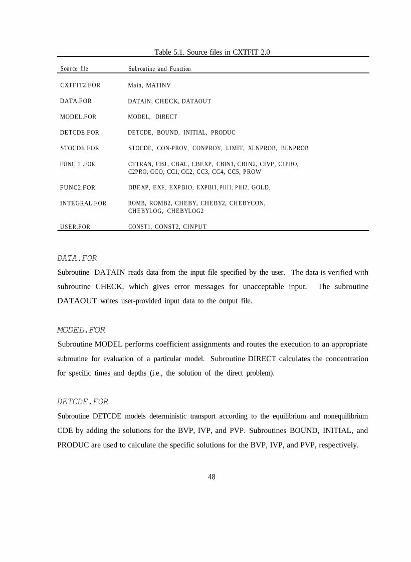
CXTFIT 2.0 consists of a main program, 22 subroutines, and 27 functions. These subprograms

are stored in nine source files. The executable program CXTFIT2 is obtained after compiling and

linking. Table 5.1 presents a list of the source files and associated subprograms.

CXTFIT2. FOR

The program unit Main controls the input, output, and parameter optimization procedures. The

subroutine MATINV performs matrix inversion for the least-squares analysis.

47

Source file

CXTFIT2.FOR

DATA.FOR

MODEL.FOR

DETCDE.FOR

STOCDE.FOR

FUNC 1 .FOR

FUNC2.FOR

INTEGRAL.FOR

Table 5.1. Source files in CXTFIT 2.0

Subroutine and Function

Main, MATINV

DATAIN, CHECK, DATAOUT

MODEL, DIRECT

DETCDE, BOUND, INITIAL, PRODUC

STOCDE, CON-PROV, CONPROY, LIMIT, XLNPROB, BLNPROB

CTTRAN, CBJ, CBAL, CBEXP, CBIN1, CBIN2, CIVP, C1PRO,C2PRO, CCO, CC1, CC2, CC3, CC4, CC5, PROW

DBEXP, EXF, EXPBIO, EXPBI1, PHI1, PHI2, GOLD,

ROMB, ROMB2, CHEBY, CHEBY2, CHEBYCON,CHEBYLOG, CHEBYLOG2

USER.FOR CONST1, CONST2, CINPUT

DATA.FORSubroutine DATAIN reads data from the input file specified by the user. The data is verified with

subroutine CHECK, which gives error messages for unacceptable input. The subroutine

DATAOUT writes user-provided input data to the output file.

MODEL.FORSubroutine MODEL performs coefficient assignments and routes the execution to an appropriate

subroutine for evaluation of a particular model. Subroutine DIRECT calculates the concentration

for specific times and depths (i.e., the solution of the direct problem).

DETCDE.FOR

Subroutine DETCDE models deterministic transport according to the equilibrium and nonequilibrium

CDE by adding the solutions for the BVP, IVP, and PVP. Subroutines BOUND, INITIAL, and

PRODUC are used to calculate the specific solutions for the BVP, IVP, and PVP, respectively.

48

STOCDE.FOR

This file calculates concentrations and variances for stochastic transport. Subroutine STOCDE

routes the execution. Function CONPROV is used for integration with respect to v, while the

function CONPROY evaluates the integrand for other stochastic parameters. Subroutine LIMIT

modifies the integration boundaries for the field-scale mean concentrations using the Newton-

Raphson method. Subroutines XLNPROB and BLNPROB quantify the single and bivariate

lognormal distributions, respectively.

FUNC1.FOR

This file evaluates many of the functions used in the analytical solutions for the equilibrium and

nonequilibrium CDE. The integrands in the nonequilibrium CDE are determined by the functions:

CTTRAN for (3.17) and (3.18), CBJ for (3.21) and (3.22), CBAL for (3.23) and (3.24), CBEXP

for (3.26) and (3.27), CBIN1 for (3.13), CBIN2 for (3.14), CIVP for the IVP (i.e., (3.34), (3.35),

(3.37), (3,38), (3.40), and (3.41)), C1PRO for (3.47) and (3.50), and C2PRO for (3.48) and (3.51).

The functions listed in Tables 2.2, 2.3, 3.2, and 3.3 are evaluated as follows: CC0 for rlE or I’,“, CC1

for G$ or G,“’ for Q= 0, CC2 for PIE or +klN, CC3 for pZE or qZN, CC4 for GIE or GIN if Q+O; CC5

for rZE or rZN; and PROD0 for GZE.

FUNC2.FOR

The remaining functions in the analytical solutions are evaluated in FUNC2.FOR. The function

DBEXP calculates the exponential function (exp), a (minimum) constraint of -100 is placed on the

value of the argument. The function EXF evaluates the product of the exponential function (exp)

and the complementary error function (erfc). EXPBIO and EXPBI1 are used to determine the

product of the exponential function (exp) and the modified Bessel functions of order zero (I,,) and one

(II), respectively (used in H, and H, as shown in Table 3.4). Functions PHI1 and PHI2 are used for

exponential solute input to calculate Qp, in (3.28) and <oZ in (3.29). Goldstein’s J-function (Table 3.4)

is determined with the function GOLD, which appears in the BVP and PVP for the nonequilibrium

CDE.

49

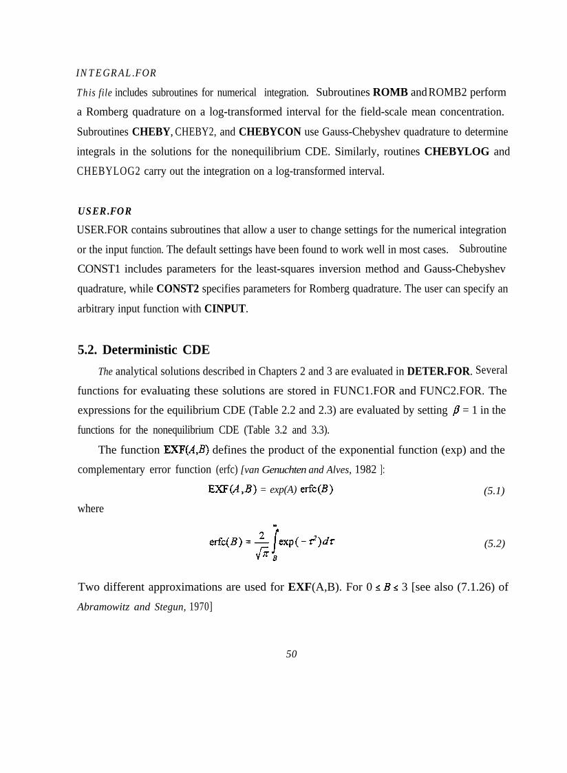
INTEGRAL.FOR

This file includes subroutines for numerical integration. Subroutines ROMB and ROMB2 perform

a Romberg quadrature on a log-transformed interval for the field-scale mean concentration.

Subroutines CHEBY, CHEBY2, and CHEBYCON use Gauss-Chebyshev quadrature to determine

integrals in the solutions for the nonequilibrium CDE. Similarly, routines CHEBYLOG and

CHEBYLOG2 carry out the integration on a log-transformed interval.

USER.FOR

USER.FOR contains subroutines that allow a user to change settings for the numerical integration

or the input function. The default settings have been found to work well in most cases. Subroutine

CONST1 includes parameters for the least-squares inversion method and Gauss-Chebyshev

quadrature, while CONST2 specifies parameters for Romberg quadrature. The user can specify an

arbitrary input function with CINPUT.

5.2. Deterministic CDE

The analytical solutions described in Chapters 2 and 3 are evaluated in DETER.FOR. Several

functions for evaluating these solutions are stored in FUNC1.FOR and FUNC2.FOR. The

expressions for the equilibrium CDE (Table 2.2 and 2.3) are evaluated by setting /? = 1 in the

functions for the nonequilibrium CDE (Table 3.2 and 3.3).

The function EXF(A,B) defines the product of the exponential function (exp) and the

complementary error function (erfc) [van Genuchten and Alves, 1982 ]:

EXF(A,B) = exp(A) erfc(B) (5.1)

whereOD

(5.2)

Two different approximations are used for EXF(A,B). For 0 < B < 3 [see also (7.1.26) of

Abramowitz and Stegun, 1970]

50

[e.g. Carnahan et al., 1969; Press et al., 1992]. Gauss-Chebyshev quadrature offers flexibility in

terms of selecting the number of integration points. We obtained accurate results with 50 integration

points for most cases (generally four to five significant digits). In some extreme cases, such as for

very small ,B and 2 or very large T, the results using 50 points may become inaccurate or incorrect.

A greater number of integration points generally results in more accurate results at the expense of

additional computer time. The latter effect is especially of concern when solving the inverse problem.

The number of integration points, MM, can be changed in subroutine CONST1.. The parameter

ICHEB in subroutine CONST1 controls the integration method. If ICHEB = 0, MM is constant at

all times. If ICHEB = 1, the program evaluates the solutions twice, namely with MM and 2xMM in

the integration routine. The number of integration points is increased until the relative change in the

solution becomes less than 0.1%. We suggest to use a set (ICHEB = 0) value of 75 for MM when

solving the inversion problem whereas ICHEB = 1 and MM = 75 appear attractive selections for the

direct problem.

An alternative method to achieve computational efficiency and accuracy is to narrow the

integration interval. The integrand in (3.17) for a Delta input (i.e.,f according to (3.15)) or in (3.20)

for a pulse input, becomes negligible for small or large t due to the exponential and complementary

error functions in l?,‘Y The modified lower (T1) and upper (T2) integration limits were obtained by

restricting integration to the domain where the argument of exponential function exceeds -30:

Tl+“+F (5.18)

(5.19)

The above modifications may significantly improve the computational efficiency without loss of

accuracy, especially for large T.

The general solution of the deterministic BVP for an arbitrary input C,, is calculated by

numerically evaluating convolution integrals (2.15) for the equilibrium CDE or (3.13) and (3.14) for

the nonequilibrium CDE. The input function needs to be specified in function CINPUT in file

USER.FOR (see also Chapter 6). Calculation of the solution should be relatively slow since a double

integral is evaluated numerically.

53

5.3. Stochastic CDE

File STOCDE.FOR assigns local-scale parameters to each stream tube and evaluates field-scale

averaged concentrations. The concentration in each stream tube is determined as described in section

5.2. Numerical integration required for the field-scale concentration and variance is carried out on

in subroutines ROMB and ROMB2 on a log-transformed interval using up to 14th order Romberg

quadrature. Since a lognormal pdf is used, log-transformation improves the efficiency and accuracy

of the numerical integration, especially for a large standard deviation, c Similar to Gauss-Chebyshev

quadrature, convergence is evaluated by comparing the integration for the kth and k+l th order. The

relative error criterion is set with variable STOPER. Convergence can usually be achieved for order

ks 10 with STOPER = 5x lO_’ unless the local Peclet number, IX/D, is high. As with the deterrninisitc

CDE, increasing the number of integration points will result in more accurate results at the expense

of more computer time. The default upper limit for k is eight, with STOPER = 5x 10” for the

evaluation of triple integrals (e.g., the stochastic nonequilibrium CDE with &+fl) or the solution

of the inverse problem. The settings for Romberg quadrature are contained in subroutine CONST2,

which appears in file USER.FOR.

To improve the computational efficiency, the upper and lower limits of integrals in the

expressions for the field-scale concentration are restricted by excluding values for v and 17 that have

a likelihood of occurrence of less than 1 x 10”. The integration limits are determined according to the

Newton-Raphson method in subroutine LIMIT. For a large standard deviation, for example o= 2

(CV = 732 %), the integration range may become too broad for numerical evaluation with this

criterion.

5.4. Parameter Estimation

CXTFIT 2.0 estimates unknown model parameters using a nonlinear least-squares optimization

approach based on the Levenberg-Marquardt method [Marquardt, 1963]. The inverse problem is

solved by fitting an appropriate mathematical solution to observed concentration data. Most of the

calculations for the least-squares analysis are carried out in the main program (Main). The model

parameters are determined by minimizing an objective function (the sum of squared residuals, SSQ)

defined as

54

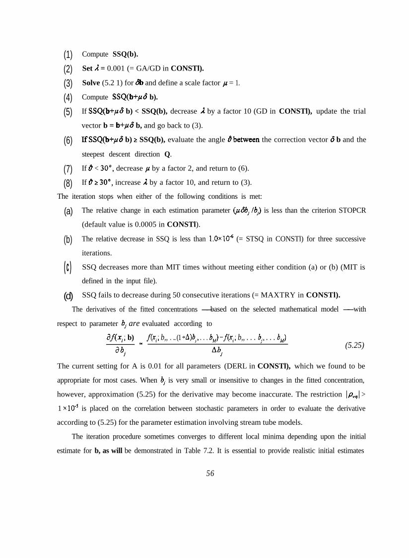
(1)(2)(3)(4)(5)

(6)

(7)(8)

Compute SSQ(b).

Set A = 0.001 (= GA/GD in CONSTl).

Solve (5.2 1) for 6b and define a scale factor ,U = 1.

Compute SSQ(b+pd b).

If SSQ(b+,uG b) < SSQ(b), decrease /z by a factor 10 (GD in CONSTl), update the trial

vector b = b+pd b, and go back to (3).

IfSSQ(b+,uS b) 2 SSQ(b), evaluate the angle 0between the correction vector 6 b and the

steepest descent direction Q.

If z9 < 30”) decrease p by a factor 2, and return to (6).

If 0 2 30”, increase A by a factor 10, and return to (3).

The iteration stops when either of the following conditions is met:

(a)

(b)

( c )

(d)

The relative change in each estimation parameter (,uShj /b,) is less than the criterion STOPCR

(default value is 0.0005 in CONSTl).

The relative decrease in SSQ is less than 1.0~ lo4 (= STSQ in CONSTl) for three successive

iterations.

SSQ decreases more than MIT times without meeting either condition (a) or (b) (MIT is

defined in the input file).

SSQ fails to decrease during 50 consecutive iterations (= MAXTRY in CONSTl).

The derivatives of the fitted concentrations --based on the selected mathematical model -- with

respect to parameter bj are evaluated according to

df(x,; b)

abj =

f(xi; b,, . .. (1 +A)$, . . . bM) -f(xi; b,, . . . b,, . . . bM)

Ab,(5.25)

The current setting for A is 0.01 for all parameters (DERL in CONSTl), which we found to be

appropriate for most cases. When bj is very small or insensitive to changes in the fitted concentration,

however, approximation (5.25) for the derivative may become inaccurate. The restriction lpV,j >

1 x lo-’ is placed on the correlation between stochastic parameters in order to evaluate the derivative

according to (5.25) for the parameter estimation involving stream tube models.

The iteration procedure sometimes converges to different local minima depending upon the initial

estimate for b, as will be demonstrated in Table 7.2. It is essential to provide realistic initial estimates

56

of the parameters, as close to the global minimum as possible. Furthermore, CXTFIT 2.0 allows the

use of maximum and minimum constraints on fitted parameters. When the new parameter value

exceeds a specified maximum or minimum value during the iteration process, the value for the

constraint is used for the next trial.

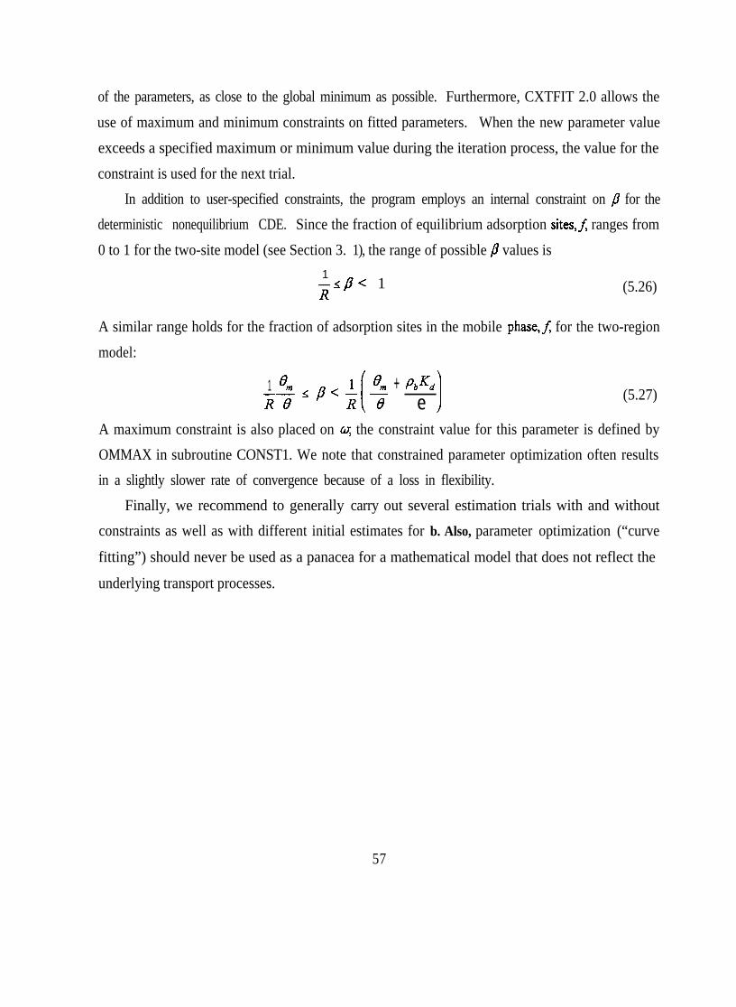
In addition to user-specified constraints, the program employs an internal constraint on /3 for the

deterministic nonequilibrium CDE. Since the fraction of equilibrium adsorption sites,f, ranges from

0 to 1 for the two-site model (see Section 3. 1), the range of possible p values is

1R 5 p< 1 (5.26)

A similar range holds for the fraction of adsorption sites in the mobile phase,f, for the two-region

model:

1 %I-- ,/?<’i IB” + PbKd

RB Re e (5.27)

A maximum constraint is also placed on 0; the constraint value for this parameter is defined by

OMMAX in subroutine CONST1. We note that constrained parameter optimization often results

in a slightly slower rate of convergence because of a loss in flexibility.

Finally, we recommend to generally carry out several estimation trials with and without

constraints as well as with different initial estimates for b. Also, parameter optimization (“curve

fitting”) should never be used as a panacea for a mathematical model that does not reflect the

underlying transport processes.

57

6. CXTFIT 2.0 USER’S GUIDE

The previous chapters provided a background of the solute transport models and of the

numerical procedures to evaluate their analytical solutions. This chapter serves as a self-contained

user manual for CXTFIT 2.0. First, the structure of CXTFIT 2.0 is outlined to give the user a quick

overview of the different modeling options. Second, the preparation of the input file is discussed.

The input is provided in a modular fashion, by using a series of blocks. Readers may only have to

read the text pertaining to the blocks for their specific application. Third, the structure of the input

and output files used for examples in this report will be reviewed. Fourth, we will compare the

differences in input format between the first version of CXTFIT [Parker and van Genuchten, 1984b]

and the current CXTFIT 2.0.

6.1. Structure of CXTFIT 2.0

CXTFIT 2.0 contains three different one-dimensional transport models: (I) the conventional

CDE; (ii) the chemical and physical nonequilibrium CDE; and (iii) a stochastic stream tube model

based on the local-scale CDE. Five different versions of the stochastic model can be selected

depending upon the type of adsorption present (equilibrium or nonequilibrium), and the type of

random transport parameters. Table 6.1 lists the characteristics of all seven models in CXTFIT 2.0;

the models are identified in the program by the parameter MODE. Deterministic transport can be

modeled with the equilibrium (MODE = 1) and nonequilibrium (MODE = 2) CDEs. The five

versions of the stream tube model are: equilibrium (MODE = 3) and nonequilibrium (MODE = 4)

adsorption with random v, D, and Kd (RD = 1); equilibrium (MODE = 5) and nonequilibrium

(MODE = 6) adsorption with random v, D, and Kd bVKd = - 1); and nonequilibrium adsorption with

random v, D, Kd and a assuming p,,,, = 1 and pvKd = -1 (MODE = 7). A stochastic parameter can be

made deterministic by setting its standard deviation to zero.

59

Table 6.1. Overview of Transport Models in CXTFIT 2.0

MODE Model Type

Deterministic CDE

Parameters Concentration Mode

1 Equilibrium

2 Nonequilibrium

Stochastic Equilibrium CDE

3 Random v, D, and Kdwith pyo= 1

5 Random v, D, and Kdwith p&-p- 1

Stochastic Nonequilibrium CDE

4 Random v, D, and Kdwith pvD= 1

6 Random v, D. and Kdwith p+g- 1

7 Random v, D, Kd, and awith pv,,= 1 and pvs- 1

Table 6.1 also presents the mode in which the concentration is detected or predicted.

Resident, flux-averaged, and total resident concentrations can be used. Although a third-type inlet

condition is generally preferable [van Genuchten and Parker, 1994], resident concentrations are also

given for a first-type inlet condition. Flux-averaged concentrations are derived from the resident

concentration for a third-type inlet condition according to (2.13). Two-types of macroscopic flux-

averaged concentration are available for stochastic transport, i.e., the ensemble average of the local-

scale flux-averaged concentration, $7, and the field-scale flux concentration, kf (= <vC,H<v>).

All analytical solutions given in Chapters 2 and 3 can be evaluated with CXTFIT 2.0. The

solution of the CDE is described as the sum of(i) a boundary value problem

value problem (IVP), and (iii) a production value problem (PVP). Table

functions that are used to characterize the BVP, IVP, and PVP.

(BVP), (ii) an initial

6.2 summarizes the

60

concentrations are obviously equal regardless of the value of NREDU; an exception is the adsorbed

concentration in case of chemical nonequilibrium. For the nonequilibrium CDE with a random Kd,

where <s/K,J~>+~>/(<K&J, the adsorbed concentration is given as -QP if NREDU = 0, and as

-QlK> if NREDU> 1.

The characteristic length, L, for nondimensional parameters is specified at the end of Block

A. CXTFIT 2.0 always uses dimensionless parameters for its internal operations; all dimensional

parameters, times, and positions in the input file are internally transformed to nondimensional

variables using the (dummy) value for L in Block A. Depending on the value for NREDU, a

transformation from the dimensionless back to the dimensional variables is carried out upon

completion of all internal operations. It is recommended to use for L a value of similar magnitude

as the observation scale (e.g., column length or soil profile depth).

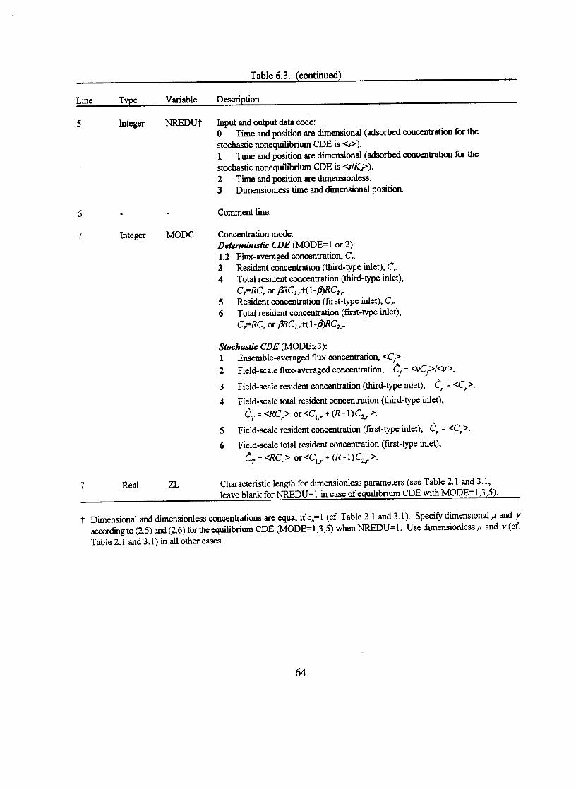
Table 6.3. Block A - Model Description

Line Type Variable Description

0

1

2, 3

4

Integer NCASE

- -

Char TITLE 1, 2

5 Integer INVERSE

5 Integer MODE

Number of cases being considered (only for the first data set).

Comment line.

Descriptive title for simulation.

Comment Line.

Calculation control code:-1 Direct problem (no results for variance in case of the stochastic CDE).0 Direct problem (results for given parameters).1 Inverse problem (parameter estimation).

Model code:1 Deterministic equilibrium CDE.2 Deterministic nonequilibrium CDE.3 Stochastic equilibrium CDE withf(v,&) and &=I.4 Stochastic nonequilibrium CDE withf(v&) and pyo’l .5 Stochastic equilibrium CDE withf(v,Q and p”g-1.6 Stochastic nonequilibrium CDE withj(v,D) and p”fl- 1.7 Stochastic nonequilibrium CDE withf(v,a), p”#-1 and ~“~=l.

63

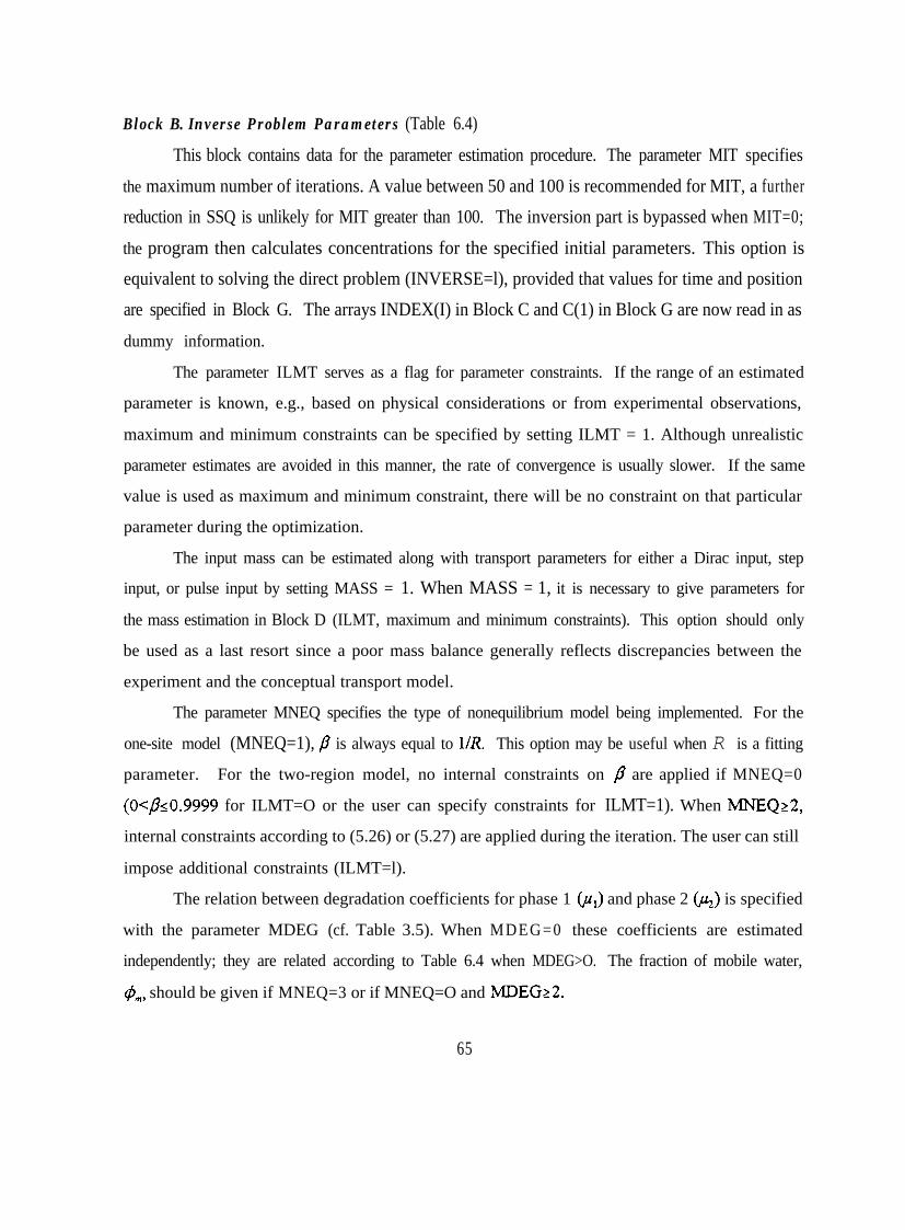
Block B. Inverse Problem Parameters (Table 6.4)

This block contains data for the parameter estimation procedure. The parameter MIT specifies

the maximum number of iterations. A value between 50 and 100 is recommended for MIT, a further

reduction in SSQ is unlikely for MIT greater than 100. The inversion part is bypassed when MIT=0;

the program then calculates concentrations for the specified initial parameters. This option is

equivalent to solving the direct problem (INVERSE=l), provided that values for time and position

are specified in Block G. The arrays INDEX(I) in Block C and C(1) in Block G are now read in as

dummy information.

The parameter ILMT serves as a flag for parameter constraints. If the range of an estimated

parameter is known, e.g., based on physical considerations or from experimental observations,

maximum and minimum constraints can be specified by setting ILMT = 1. Although unrealistic

parameter estimates are avoided in this manner, the rate of convergence is usually slower. If the same

value is used as maximum and minimum constraint, there will be no constraint on that particular

parameter during the optimization.

The input mass can be estimated along with transport parameters for either a Dirac input, step

input, or pulse input by setting MASS = 1. When MASS = 1, it is necessary to give parameters for

the mass estimation in Block D (ILMT, maximum and minimum constraints). This option should only

be used as a last resort since a poor mass balance generally reflects discrepancies between the

experiment and the conceptual transport model.

The parameter MNEQ specifies the type of nonequilibrium model being implemented. For the

one-site model (MNEQ=1), ,0 is always equal to l/R. This option may be useful when R is a fitting

parameter. For the two-region model, no internal constraints on ,8 are applied if MNEQ=0

(0<,&0.9999 for ILMT=O or the user can specify constraints for ILMT=1). When MNEQ22,

internal constraints according to (5.26) or (5.27) are applied during the iteration. The user can still

impose additional constraints (ILMT=l).

The relation between degradation coefficients for phase 1 (&) and phase 2 (,uJ is specified

with the parameter MDEG (cf. Table 3.5). When MDEG=0 these coefficients are estimated

independently; they are related according to Table 6.4 when MDEG>O. The fraction of mobile water,

@,, should be given if MNEQ=3 or if MNEQ=O and MDEG22.

65

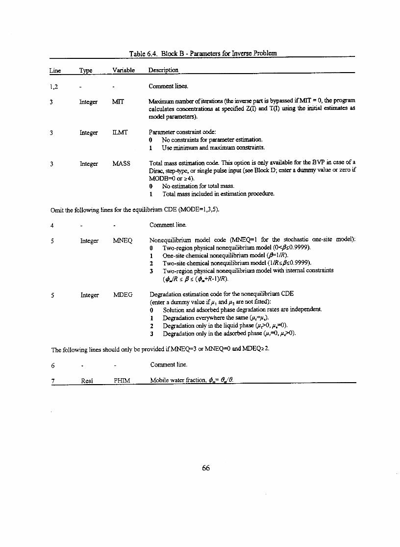
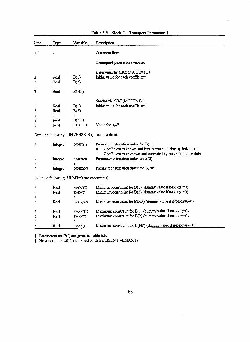
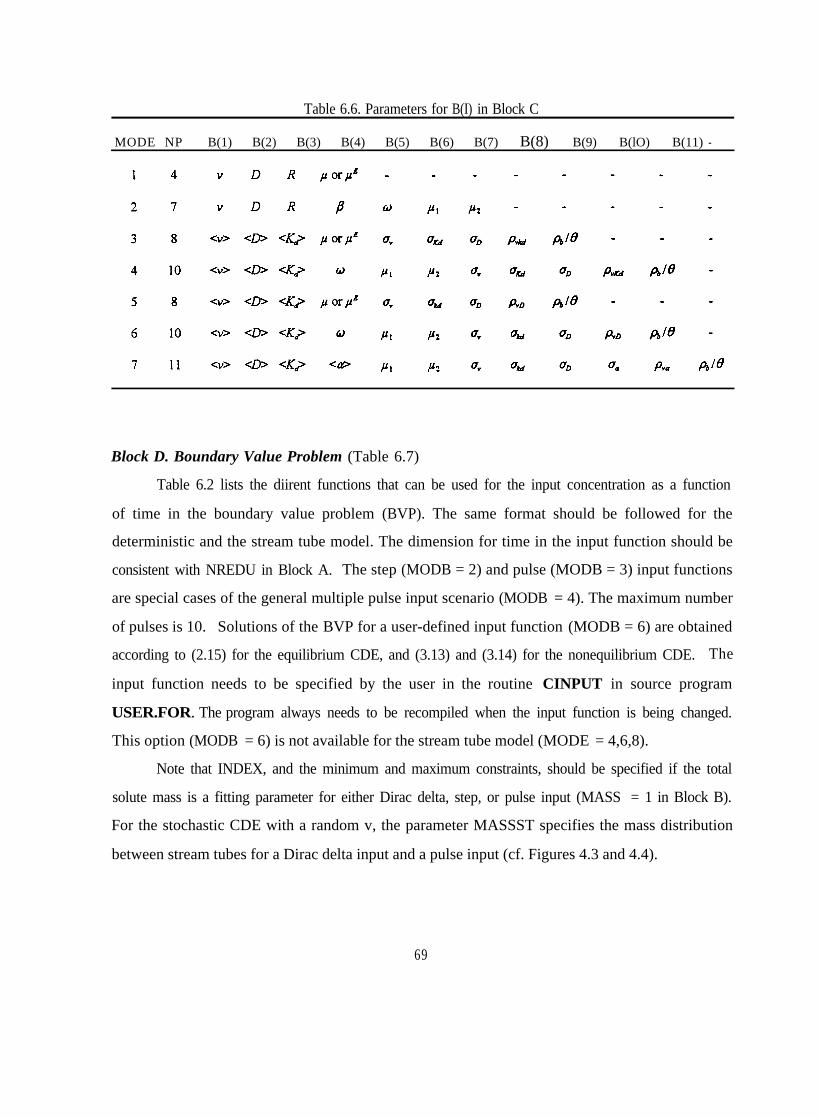
Table 6.6. Parameters for B(I) in Block C

MODE NP B(1) B(2) B(3) B(4) B(5) B(6) B(7) B(8) B(9) B(lO) B(11) -

Block D. Boundary Value Problem (Table 6.7)

Table 6.2 lists the diirent functions that can be used for the input concentration as a function

of time in the boundary value problem (BVP). The same format should be followed for the

deterministic and the stream tube model. The dimension for time in the input function should be

consistent with NREDU in Block A. The step (MODB = 2) and pulse (MODB = 3) input functions

are special cases of the general multiple pulse input scenario (MODB = 4). The maximum number

of pulses is 10. Solutions of the BVP for a user-defined input function (MODB = 6) are obtained

according to (2.15) for the equilibrium CDE, and (3.13) and (3.14) for the nonequilibrium CDE. The

input function needs to be specified by the user in the routine CINPUT in source program

USER.FOR. The program always needs to be recompiled when the input function is being changed.

This option (MODB = 6) is not available for the stream tube model (MODE = 4,6,8).

Note that INDEX, and the minimum and maximum constraints, should be specified if the total

solute mass is a fitting parameter for either Dirac delta, step, or pulse input (MASS = 1 in Block B).

For the stochastic CDE with a random v, the parameter MASSST specifies the mass distribution

between stream tubes for a Dirac delta input and a pulse input (cf. Figures 4.3 and 4.4).

69

Table 6.7. Block D - Boundary Value Problem?

Line Type Variable Description

1,2 -

(0) Solute free water input

3 Integer MODB

(1) Dirac Delta input

3 Integer MODB

4 Real PULSE( 1)

4 Real MASSST

Comment lines.

0

1

mJv or -3n,+v> for dimensional 6(t),Md or 442 for dimensionless 8(T).

Mass distribution index for the stochastic CDE (leave blank for the deterministicCDE, i.e., MODEs2).0 Amount of solute in each tube is proportional to v (m,=v<m@v>).1 Amount of solute in each tube is constant regardless of v (m,=<mfl).

Omit the following if INVERSE=0 (Block A) or MASS=0 (Block B).

5 Integer INDEX(NP+l) Parameter estimation index for solute mass (=B(NP+l)).0 Coefficient is known and kept constant.1 Coefficient is assumed to be unknown and fitted to data

Omit the following if there are no constraints (ILMT=0, Block B).

6 Real BMIN(NP+1) Minimum constraint for B(NP+1) (dummy value if INDEX(NP+1)=0).

7 Real BMAX(NP+1) Maximum constraint for B(NP+1) (dummy value if INDEX(NP+1)=0).

(2) Step input

3 Integer MODB 2

4 Real PULSE( 1) Input concentration,l,.

Omit the following if INVERSE=0 (Block A) or MASS=0 (Block B).

5 Integer INDEX(NP+1) Parameter estimation index for input concentration (=B(NP+1)).0 Coefficient is known and kept constant.1 Coefficient is assumed to be unknown and fitted to the data.

Omit the following if there are no constraints (ILMT=O, Block B).

6 Real BMIN(NP+1) Minimum constraint for B(NP+1) (dummy value if INDEX(NP+1) =0).

7 Real BMAX(NP+l) Maximum constraint for B(NP+l) (dummy value if INDEX(NP+l) =0).

70

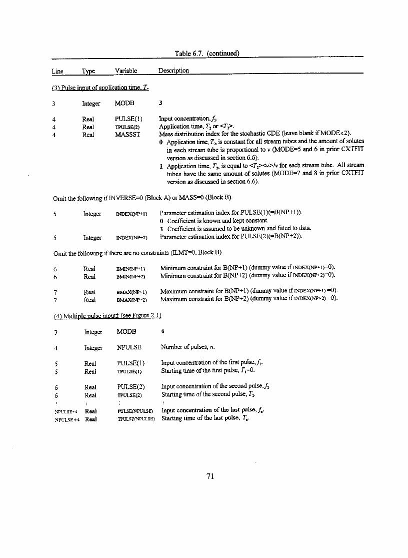
Table 6.8. Block E - Initial Value Problemf

Line Type Variable Description

1,2 - comment lines.

(0) Zero initial concentration

3 Integer MOD1 0

( 1) Constant initial concentration

3 Integer MOD1 1

4 Real CINI(1) Concentration, U,.

(2) Stepwise Initial Distribution? (see Figure 2.2)

3 Integer MOD1 2

4 I n t e g e r NINI Number of steps, n.

5 Real CINI(1) Concentration of the first step, U,.5 Real ZINI(1) Starting position of the first step, Z,=O.

6 Real CINI(2) Concentration of the second step, U,.6 Real ZINI(2) Starting position of the second step, 2,.

NINI+4 Real CINI(NINI) Concentration of the last step, U,.NINI+4 Real ZINI(NINI) Starting position of the last step, 2,

(3) Exponential initial distribution. u, + u, exp (-A’ Z)

3 Integer MOD1 3

4 Real CINI(1) Value of U,.4 Real CINI(2) Value of U,.4 Real ZINI(1) Value of A’.

(4) Dirac delta initial condition. m,lB6(x - x,1+ U,. or M, &iZ - 2,) + U,

3 Integer MOD1 4

4 Real CINI(2) Value of m,/8 or M,.4 Real ZINI(2) Value of x, or 2, (x, , Z, ~0 when MODC=5,6).4 Real CINI( 1) Value of U,.

t The dimension for depth in the initial condition should be specified according to the value of NREDU (Block A).$ Zero and constant initial concentrations are special cases of a stepwise initial distribution.

73

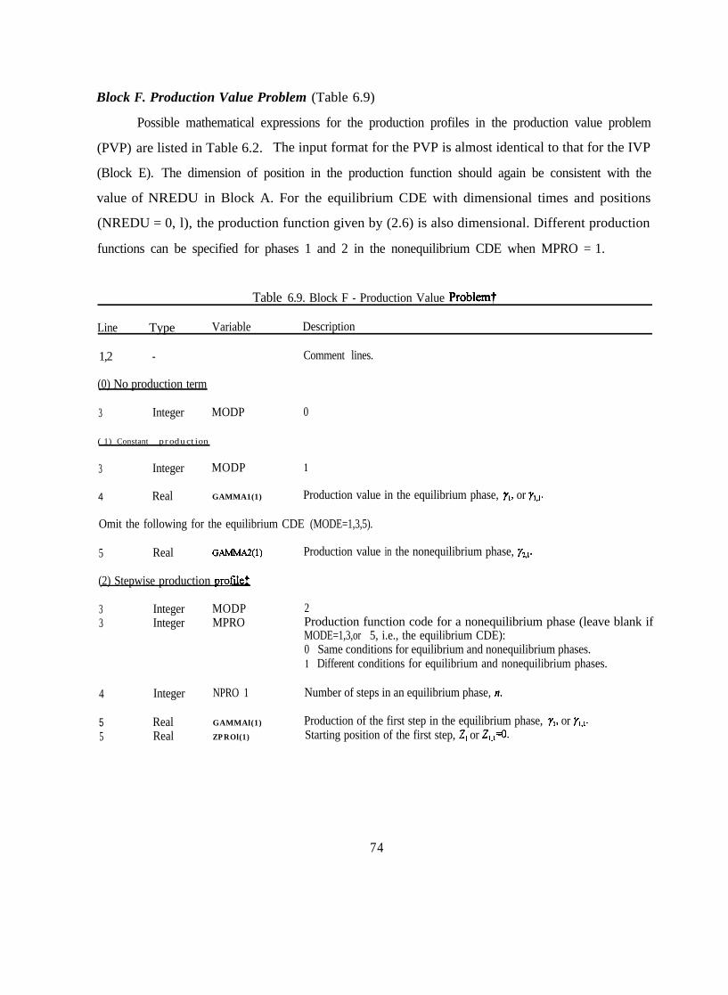
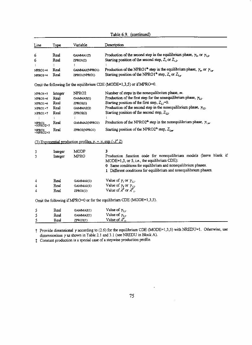
Block F. Production Value Problem (Table 6.9)

Possible mathematical expressions for the production profiles in the production value problem

(PVP) are listed in Table 6.2. The input format for the PVP is almost identical to that for the IVP

(Block E). The dimension of position in the production function should again be consistent with the

value of NREDU in Block A. For the equilibrium CDE with dimensional times and positions

(NREDU = 0, l), the production function given by (2.6) is also dimensional. Different production

functions can be specified for phases 1 and 2 in the nonequilibrium CDE when MPRO = 1.

Table 6.9. Block F - Production Value Problemt

Line Type

1,2 -

Variable Description

Comment lines.

(0) No production term

3 Integer MODP 0

( 1) Constant production

3 Integer MODP 1

4 Real GAMMA1(1) Production value in the equilibrium phase, y,, or y,.,.

Omit the following for the equilibrium CDE (MODE=1,3,5).

5 Real Production value in the nonequilibrium phase, yfl.

(2) Stepwise production profiie$

3 Integer MODP3 Integer MPRO

2Production function code for a nonequilibrium phase (leave blank ifMODE=1,3,or 5, i.e., the equilibrium CDE):0 Same conditions for equilibrium and nonequilibrium phases.1 Different conditions for equilibrium and nonequilibrium phases.

4 Integer NPRO 1 Number of steps in an equilibrium phase, n.

5 Real GAMMAl(1) Production of the first step in the equilibrium phase, y,, or y,.,.5 Real ZPROl(1) Starting position of the first step, 2, or Z,,,=O.

74

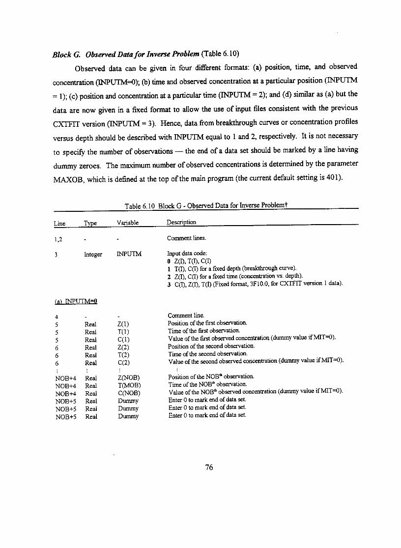
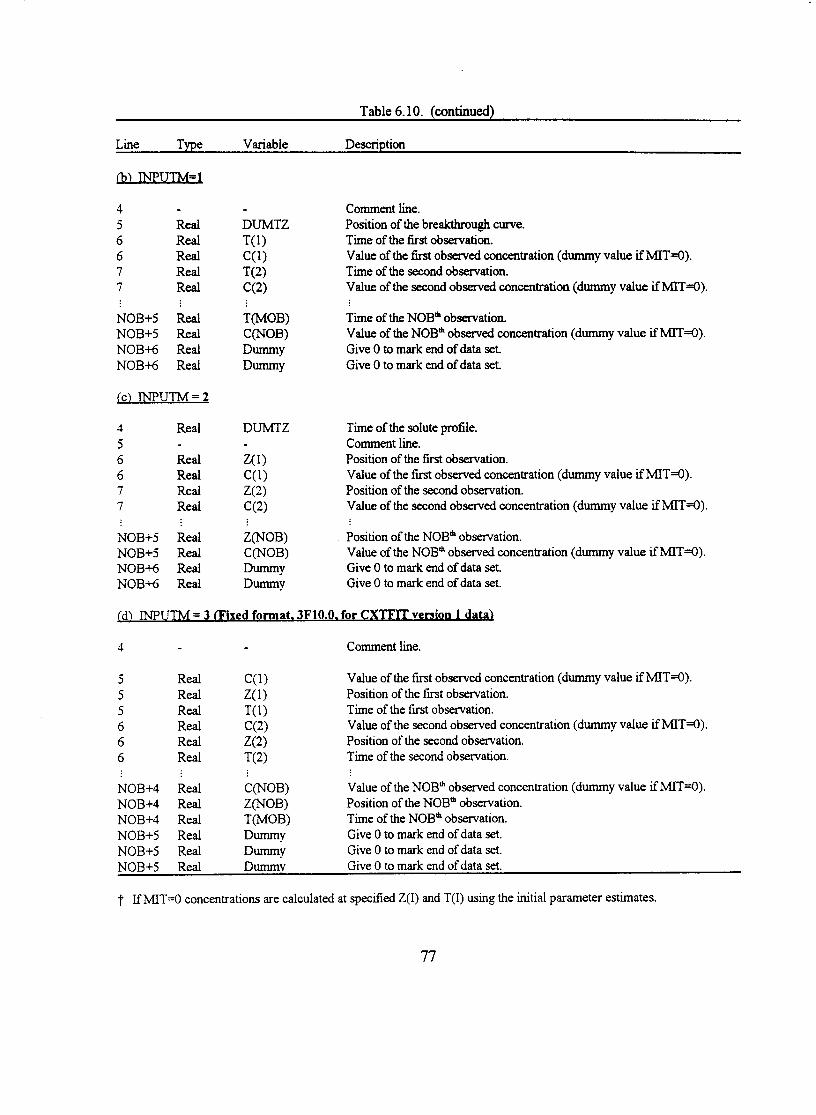
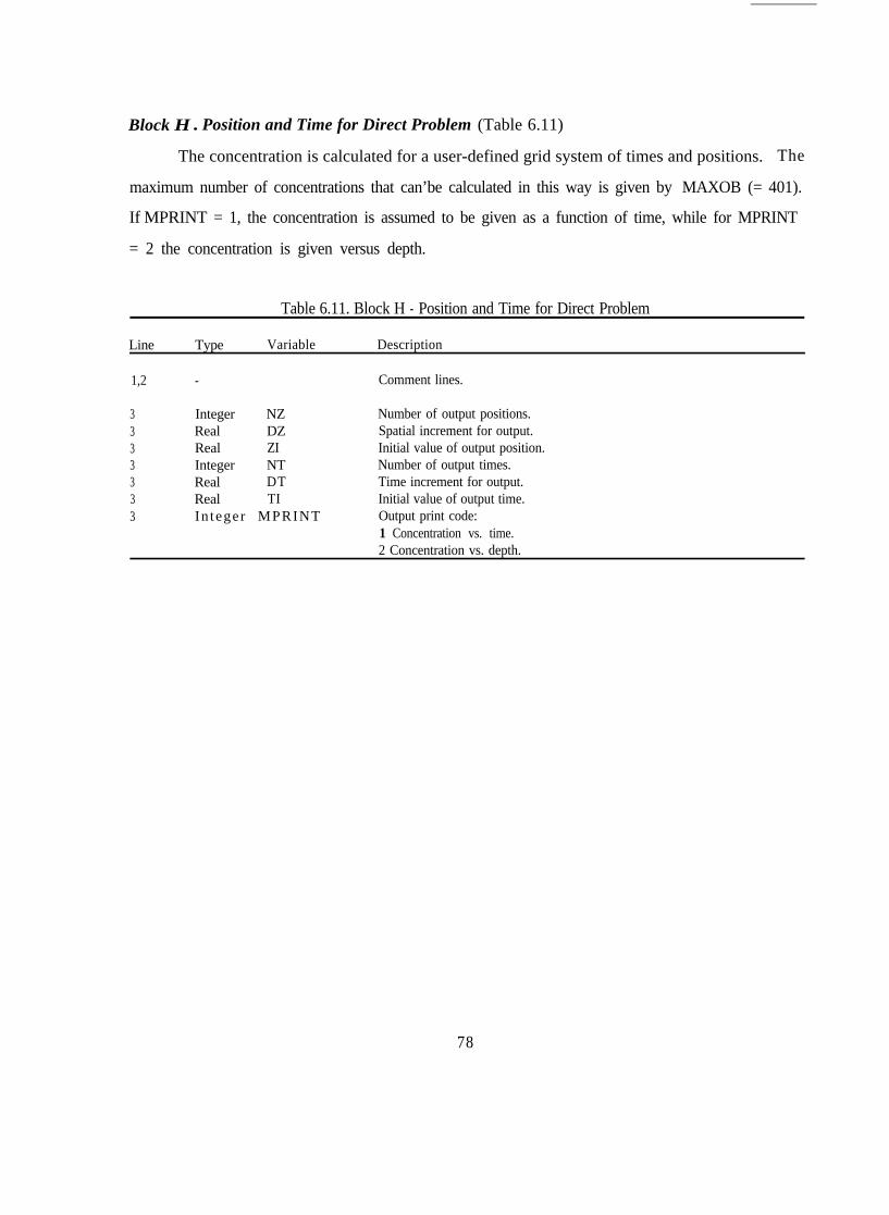
Block H . Position and Time for Direct Problem (Table 6.11)

The concentration is calculated for a user-defined grid system of times and positions. The

maximum number of concentrations that can’be calculated in this way is given by MAXOB (= 401).

If MPRINT = 1, the concentration is assumed to be given as a function of time, while for MPRINT

= 2 the concentration is given versus depth.

Table 6.11. Block H - Position and Time for Direct Problem

Line Type Variable Description

1,2 - Comment lines.

3 Integer NZ Number of output positions.3 Real DZ Spatial increment for output.3 Real ZI Initial value of output position.3 Integer NT Number of output times.3 Real DT Time increment for output.3 Real TI Initial value of output time.3 In teger MPRINT Output print code:

1 Concentration vs. time.2 Concentration vs. depth.

78

6.3. Example Input and Output Files

We will present in this section some typical examples of direct and inverse problems. All input

and output files for the examples are provided on the distribution diskette.

6.3.1. Direct Problem

Tables 6.12 and 6.13 are input and output files for the deterministic nonequilibrium CDE (cf.

Figure 7.6a). Block H in the input file is used to specify the grid of times and positions for which

concentrations are to be calculated. The parameter NCASE, on the first line of the input file,

specifies the number of cases considered. The output f i l e shows the conditions for the simulation as

well as calculated results for times and positions specified in Block H. The concentration is given as

a function of time if MPRINT = 1 (Block H), or as a function of position (distance) if MPRINT = 2.

To check the mass balance, zero th time (MPRINT = 1) and depth (MPRINT = 2) moments are

calculated according to:n - l

sum (C*dT) = c (ci + Ci,,)A7-/2i=l

(6.2)

n-l

Sum(C*dZ) = c ( ci + Ci+r)A2/2 (6.3)i=l

1Table 6.12. Input File for Figure 7.6a

+++ BLOCK A: MODEL DESCRIPTION C+~Cllllf~~*1~~Ct*l~~~~*~~~~~~~~~~~~~~~~~~~Fig7-6a. Two-site CDE (Alpha=0.08,f=0.7)Effect of the fraction of equilibrium site, fINVERSE MODE NREDU

0 2 1MODC ZL

1 50*** BLOCK C: TRANSPORT PARAMETERS **~~~+tt**ltt~*+fttt~~~~~~~~~~~~~~~~~~*~

V D R Beta omega Mu1 Mu220. 10. 5.0 0.44 0.56 0.0 0.0

++ BLOCK D: BVP; MODB=O ZERO; =1 Dirac; =2 STEP: =3 A PULSE ++**C+*t+fC++MODB =4 MULTIPLE; =5 EXPONENTIAL; =6 ARBITRARY1

1.0+*+ BLOCK E: IVP; MODI=O ZERO; =l CONSTANT; =2 STEPWISE; =3 EXPONENTIAL ++MODI

0+++ BLOCK F: PVP; MODP=O ZERO; =l CONSTANT; =2 STEPWISE; =3 EXPONENTIAL **

MODP0

++* BLOCK H: POSITION AND TIME FOR DIRECT PROBLEM C+t~t~Ct+~*ifCCf~iCt~~~~NZ DZ ZI NT DT TI MPRINT

1 1.0 50.0 101 0.2. 0.0 1

79

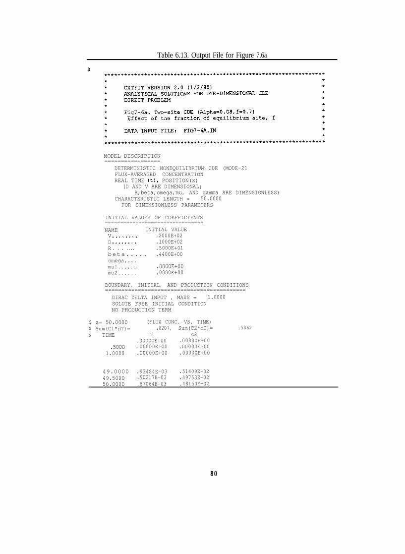
Table 6.13. Output File for Figure 7.6a

MODEL DESCRIPTION=================

DETERMINISTIC NONEQUILIBRIUM CDE (MODE-21FLUX-AVERAGED CONCENTRATIONREAL TIME (t), POSITION(x)

(D AND V ARE DIMENSIONAL;R,beta,omega,mu, AND gamma ARE DIMENSIONLESS)

CHARACTERISTIC LENGTH = 50.0000FOR DIMENSIONLESS PARAMETERS

INITIAL VALUES OF COEFFICIENTS================================NAME INITIAL VALUEV . . . . . . . . .2000E+02D . * . . . . . . .l000E+02R . . . .... .5000E+0lbeta..... .4400E+00omega.... .5600E+00mu1...... .0000E+00mu2...... .0000E+00

BOUNDARY, INITIAL, AND PRODUCTION CONDITIONS===========================================

DIRAC DELTA INPUT , MASS = 1.0000SOLUTE FREE INITIAL CONDITIONNO PRODUCTION TERM

$ z= 50.0000 (FLUX CONC. VS. TIME)$ Sum(C1*dT)= .8207, Sum(C2*dT)= .5062$ TIME C1 c2

..0000 .00000E+00 .00000E+00

.5000 .00000E+00 .00000E+001.0000 .00000E+00 .00000E+00

49.0000 .93484E-03 .51409E-0249.5000 .90217E-03 .49753E-0250.0000 .87064E-03 .48150E-02

80

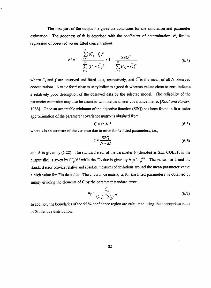
b.~,min = bj,jft - tN-M,0.975 (‘J$‘~ (6.8)b.J.IllUC = bjJit + tN-M,O.975 (cy (6.9)

where bjfit is the fitted parameter value, and t,,,_M,,,975 is the value of the t distribution for confidence

level 0.95 with N - M degrees of freedom.

It should be noted that since (6.5), (6.8), and (6.9) are based on linear regression analysis,

they hold only approximately for the nonlinear analysis as was discussed by Kool und Parker [ 1988].

However, (6.8) and (6.9) will yield reasonable approximations for individual parameter confidence

intervals if no constraints are used and bjst represents the true global minimum of the objective

function.

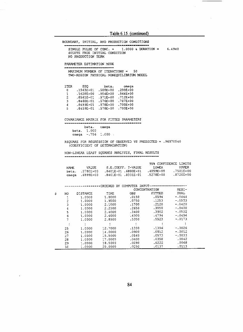
Table 6.15. Output File for Figure 7.9b

MODEL DESCRIPTION=================

DETERMINISTIC NONEQUILIBRIUM CDE (MODE=2)FLUX-AVERAGED CONCENTRATIONREDUCED TIME (T), POSITION(Z)

(ALL PARAMETERS EXCEPT D AND V ARE DIMENSIONLESS)CHARACTERISTIC LENGTH = 30.0000

FOR DIMENSIONLESS PARAMETERS

INITIAL VALUES OF COEFFICIENTS==============================NAME INITIAL VALUE FITTINGV . . . . . . . . .3850E+02 ND . . . . . . . . .1550E+02 NR . . . . . . . . .3900E+01 Nbeta..... .5000E+00 Yomega.... .2000E+00 Ymu1...... .0000E+00 Nmu2...... .0000E+00 N

83

6.4. CXTFIT 1.0

This section outlines the difference in input format for CXTFIT 2.0 and its predecessor,

version 1 [Parker and van Genuchten, 1984]. This information is included to quickly familiarize

users of the prior CXTFIT program with the current version. All functions in CXTFIT 1 .O are also

included in version 2, except for parameter estimation of the constant production term, y, in the

equilibrium CDE (MODE = 1,2 in version 1). Many examples were tested using the two versions;

identical results were obtained in most cases, while at times the parameter optimization was slightly

better for CXTFIT 2.0. Changes in the input structure are outlined below.

Model Type and Concentration Mode

In version 1, the parameter MODE specified model type and concentration mode. In version

2, the parameters MODE and MODC in Block A specify the model type and the concentration mode,

respectively. The resident concentration in version 1 is identical to the resident concentration for a

third-type inlet condition in version 2 (MODC = 3). Field-scale flux averaged concentrations in

version 1 are specified by MODC = 2 in CXTFIT 2.0 (cf. Table 6.1).

Estimation of Solute Application Time

The pulse duration was estimated as a transport parameter in version 1. In this version, the

user also needs to set MASS = 1 in Block B and INDEX = 1 for the application time in Block D.

Degradation Coefficient

The degradation coefficient ,u for the deterministic CDE was always dimensional in version

1. As explained in Block C, ,u may be dimensional or dimensionless in version 2, depending upon the

value of NREDU in Block A.

85

Characteristic Length

The characteristic length L for nondimensional parameters in version 1 was defined internally

as the maximum value of the independent variable, x. Instead, a value for L now has to be entered

by the user in Block A. This modification allows greater flexibility, while nondimensional parameters,

such as w, can also be made independent from the maximum depth for a particular set of

observations.

Stochastic Model with Random v

The stochastic model in version 1 consisted of a stream tube model with random pore-water

velocity, v. Additional stochastic parameters can be used in version 2 as discussed in Chapter 4. The

case of only a stochastic v can be modeled in CXTFIT 2.0 by setting the other standard deviations

of all other parameters to zero.

Constant Local-Scale Dispersivity

In version 1 only a constant dispersivity, /t, could be used (see (4.25)). To do this in version

2, identical initial estimates for a, and a, (MODE = 3) should be entered to keep /1 constant during

the parameter estimation in process. The input parameter is CD>.

Stochastic Model for Pulse Input of Constant Duration

A constant application time for the stochastic model (MODE = 5,6 in version 1) can now be

given by setting MASSST = 0 for MODB = 3 in Block D (see Figure 4.4).

Stochastic Model with Constant Mass

The stochastic model with constant mass (MODE = 7,8 in version 1) can be evaluated in

version 2 by setting MASSST = 1 for MODB = 3 in Block D.

86

7. EXAMPLE PROBLEMS

This chapter contains several examples to illustrate the application of CXTFIT 2.0 to different

transport scenarios. Both solutions of the direct and the inverse problem will be discussed for several

types of boundary value (BVP), initial value (IVP), and production value (PVP) problems. A third-

type inlet condition is used in all example problems, while concentrations in the examples are always

normalized with respect to the input concentration or initial concentration (Tables 2.1 and 3.1). The

input and output files for each example can be found on the distribution diskette.

7.1. Deterministic Equilibrium CDE (MODE = 1)

7.1.1. Direct Problem

The first two examples deal with the solution of the direct problem for the equilibrium CDE.

Figure 7.1 illustrates the effect of the first-order decay constant p, as given by (2.9, on solute

2.0

1.5

0’ 1.0

0.5

0.0

I I I I

- t=7.5d

Fig. 7.1. Effect of the first-order decay constant, ,u, on calculated C,-profiles.

87

distributions. The resident concentration was calculated 7.5 d after applying a single pulse input at

t = 0 with duration tt = 5 d to a solute-free soil profile assuming v = 25 cm d-r, D = 37.5 cm’d-‘, R

= 3, and a constant rate of production y= 0.5 mg kg-’ d-r [van Genuchten, 1981a]. Notice that

when ,U increases, the concentration decreases as a result of the rise in degradation. Concentrations

were evaluated according to (2.34) for ,u = 0 d“ while (2.33) was used for pu>O 6’.

Differences between resident (C,) and flux-averaged (c;> concentrations for the BVP have

been discussed extensively by several authors [cf. Kreft and Zuber, 1978; Jury and Roth, 1990; van

Genuchten and Parker, 1984b]. We will illustrate the differences in concentration mode for the IVP

[Toride et al., 1993b]. Figure 7.2 shows C, and Cr as a function of relative distance, 2, at

dimensionless time T = 0.05 for two values of P when solute-free water is applied to a soil having a

stepwise initial resident distribution as indicated by the dashed line. Dispersive transport dominates

convective transport when P = 2, causing considerable spreading to occur in both the upstream and

downstream directions (Figure 7.2a). Notice that at this small time (T = 0.05), Cr is negative for

2~0.5, and greater than unity (the initial resident concentration) for Z= 1. These somewhat odd

results are a direct result of the definition of C’ according to (2.13). Since the solute flux, J,, and the

water flux, J, are vectors, Cr becomes negative when the directions of these two fluxes are opposite.

The negative Cr near the surface is the result of an upward dispersive solute flux in spite of a

downward convective solute flux. Similarly, C/ is greater than C, if the gradient of C; becomes

negative. For relatively large negative gradients such as those in Figure 7.2 around 2 = 1, C,can

become greater than the initial resident concentration C,(Z,O). Notice from Figure 7.2b that the

differences between C,and C, become smaller for an increased Peclet number, P.

88

Table 7.1. Pore-Water Velocity, v, Dispersion Coeffkient, D, andDispersivity, I, Obtained by Fitting the Data of Figure 7.2

Depth V D Acm cmd-' cm’d-’ cm

(a) Saturated (B= 0.3)

11 2.45 0.154 0.06317 2.51 0.126 0.05023 2.51 0.110 0.044

(b) Unsaturated (8= 0.12)

11 0.258 0.0357 0.1417 0.254 0.0393 0.1523 0.249 0.0429 0.17

The input mass can be used as a fitting parameter by setting MASS = 1 for a Dirac delta input

and a pulse input. For a pulse input either the application time or the input concentration can be

estimated. Figure 7.4 shows observations and the breakthrough curve obtained by fitting the duration

of the application for a pulse input, t2, in addition to v and D. The concentration was measured with

a TDR probe at a depth of 10 cm for a pulse application of KCl solution to an undisturbed sandy soil

column [Mallants et al., 1994]. The fitted parameters are v = 2.34 cm d-‘, D = 12.8 cm2 d-‘, and t,

= 0.8 h. We again note that mass balance errors are likely to have an adverse effect on the estimation

of all transport parameters.

91

Figure 7.7b presents two BTCs for a pulse input of 5 days using the same set of parameters

as in Figure 7.7a. Differences between the BTCs predicted with the two different data sets are more

pronounced for the pulse input than for the Dirac input. The enhanced tailing for the pulse input will

likely somewhat improve the estimated transport parameters in the two-site model.

Since the two-region nonequilibrium model is mathematically identical to the two-site model

(cf. Section 3.1.3), we may conclude from the above that different sets of R, a: and 8, also may lead

to nearly identical concentration profiles. For reactive solutes, the fraction, f, of adsorption sites in

contact with the mobile liquid phase will cause additional uncertainty in the parameter estimation.

When the BTCs for reactive solutes are analyzed in terms of the two-region model, it is best to

estimate 19, from data for a nonreactive tracer (see also Figure 7.9).

The last example involving a direct problem concerns deterministic nonequilibrium transport

as described by an initial value problem (IVP). Figure 7.8 shows equilibrium (C,) and nonequilibrium

(CJ resident concentration profiles at T = 1 .O for three values of the partitioning coefficient /?. The

example involves the application of a solute-free solution to a soil with a stepwise initial solute

distribution (dashed line in Fig. 7.8), assuming P = 10, R = 2, o = 1, and ,u~ = ,uz = 0.2. Figure 7.8

shows that solutes are transported more slowly when pis relatively small, i.e., when a relatively large

amount of solute resides in the nonequilibrium phase. Hence, leaching is not as effective when /3 is

small. Notice also that the discontinuity in the nonequiiibrium concentration, C,, persists much longer

when /?is small. The discontinuity persists because solute removal and subsequent leaching from the

nonequilibrium phase can only occur indirectly through the equilibrium phase after the solute has

kinetically desorbed from the adsorbed to the solution phase (the one- or two-site adsorption models),

or has diised from immobile to mobile water (the two-region model). The nonequilibrium profiles

closely resemble the equilibrium when p is large because of increased opportunity for the relatively

small amount of solute in the nonequilibrium phase to move to the equilibrium phase.

96

7.2.2. Parameter Estimation

Several examples below illustrate the use of CXTFIT 2.0 to estimate parameters involving the

nonequilibrium deterministic model. The first example deals with two-region nonequilibrium

transport of tritiated water through a Glendale clay loam Experiment 3-2 of van Genuchten, 1974].

A ‘HZ0 pulse of duration 2; = 3.102 was applied to a 30-cm long column, and the BTC was

determined from the effluent. The volumetric water content, 0, was 0.454 while the pore-water

velocity, v, was equal to 37.5 cm d-‘. Assuming that R = 1 for 3H,0, we only have to estimate p(=

6,/8) and o from the measured BTC. Figure 7.9a compares the observed and fitted BTCs. The

number of pore volumes, T, was used as the dimensionless time in this example (NREDU = 2). We

emphasize that v (= v,,, 8,,/9 and D (= D,,, 6,/B) are used as the unknown input parameters, instead

of v, and D ,,,, which appear in the two-region physical nonequilibrium model (Table 6.7). The fitted

values were D = 15.5 cm2 d-‘, 8,,,/8= 0.822, and o= 0.85. These values correspond to v,,, = 45.6

cm d-‘, D, = 18.9 cm2 d-r, and a= 0.48 d-r.

A pulse of boron tracer was also applied for T, = 6.494 pore volumes to the same column as

used in Figure 7.9a [Exp. 3-l of van Genuchten, 1974].. The estimated parameters were v = 38.5 cm

d-’ andR = 3.9 (&= 1.04 g-’ cm3, pb = 1.222 g cme3, and 8= 0.445). We assumed that D and 19,,/6

are identical for boron and 3H20 (Figure 7.9a). Figure 7.9b shows the observed and fitted BTCs with

parameters /?= 0.578 and o= 0.70 (a= 0.40 d-r). Substituting B,,,JB= 0.822, as obtained from the

3H20 BTC, into the expression for p (cf. Table 3.1) yieldsf= 0.49 for the fraction of sorption sites

in contact with the mobile phase.

The boron data are the same as those shown in Figure 5 of the previous CXTFIT manual

[Parker and van Genuchten, 1984b] when four parameters (D, R, p, and o) were estimated. Table

7.2 shows the effect of having different initial estimates and number of unknown parameter on the

optimization of the boron BTC given in Figure 7-9b - similar information was previously shown

in Table 3 of Parker and van Genuchten [ 1984b].. Two different sets of initial estimates were used

to estimate either two (i.e., ,0and o, with D obtained by fitting the ‘H,O BTC) or three (i.e., D, ,O,

and o) parameters. For the two-parameter estimation, ,0 and o converged to almost identical results

regardless of the initial estimates. If D was also optimized, the final results depended greatly on the

initial estimates. The results for the three-parameter estimation in Table 7.2 were quite dissimilar

98

although only the initial value for /I was different in the two examples. Since the product flR

determines the number of pore-volumes, T, at which the tracer initially appears in the effluent, it is

important to provide a reasonable initial estimate for PR. IfR is fitted as well - in addition to D,

j?, and o such as in Table 3 in Parker and van Genuchten [ 1984b] - the likelihood that the

optimization does not converge to the correct solution will increase. Figure 7.7 suggests that

different parameter sets can yield very similar curves. This occurs when the response surface (i.e.,

the objective function, SSQ(b)) has a flat surface near the global minimum or when multiple local

minima exist.

1.0

G- 05.

I

(a) 3H2O- Fitted

. Observed

0 2 4 6 8

Fig 7.9. Breakthrough curves for a Glendale clay loam described by the two-regionphysical nonequilibrium model for nonreactive 3H,0 and reactive boron.

99

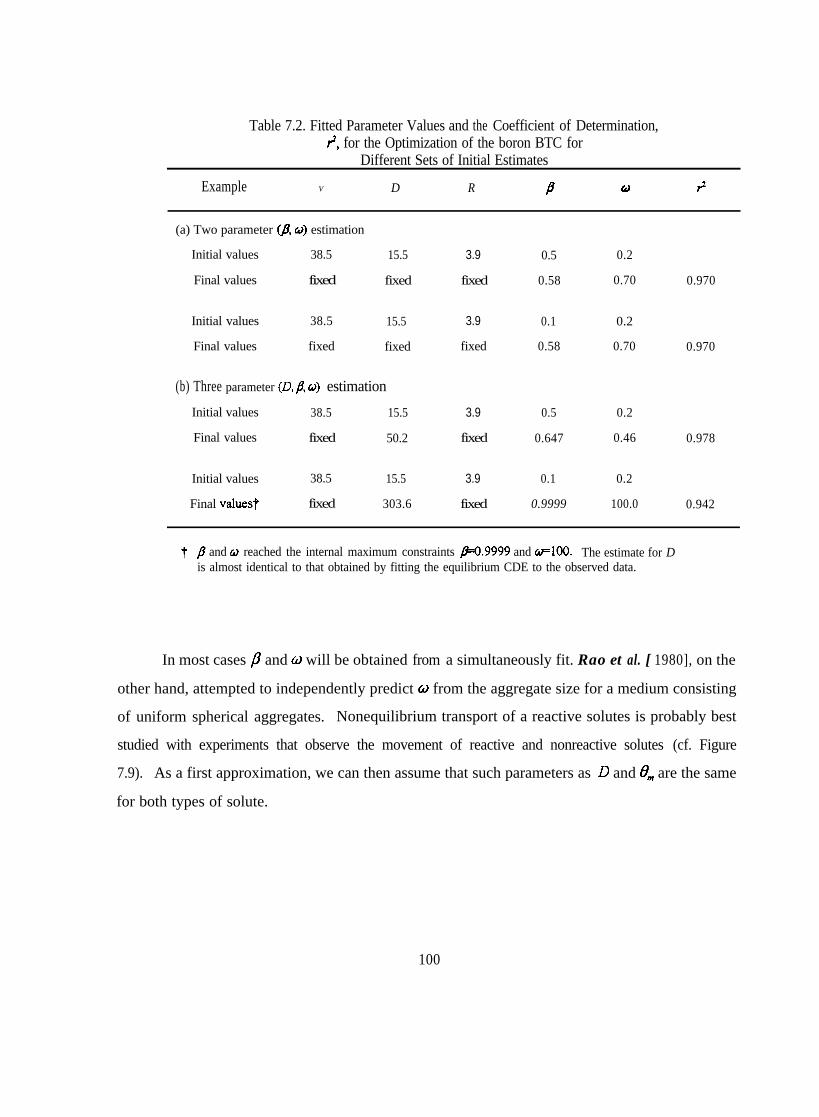
Table 7.2. Fitted Parameter Values and the Coefficient of Determination,?, for the Optimization of the boron BTC for

Different Sets of Initial Estimates

Example V D R B 0 IJ

(a) Two parameter @, o) estimation

Initial values 38.5 15.5

Final values fixed fixed

Initial values 38.5 15.5 3.9 0.1 0.2

Final values fixed fixed fixed 0.58 0.70 0.970

(b) Three parameter (0, P, o) estimation

Initial values 38.5 15.5

Final values fixed 50.2

Initial values 38.5 15.5 3.9 0.1 0.2

Final values? fixed 303.6 fixed 0.9999 100.0 0.942

3.9 0.5 0.2

fixed 0.58 0.70 0.970

3.9 0.5

fixed 0.647

0.2

0.46 0.978

t p and o reached the internal maximum constraints /?=0.9999 and ~100. The estimate for Dis almost identical to that obtained by fitting the equilibrium CDE to the observed data.

In most cases ,0 and w will be obtained from a simultaneously fit. Rao et al. [ 1980], on the

other hand, attempted to independently predict o from the aggregate size for a medium consisting

of uniform spherical aggregates. Nonequilibrium transport of a reactive solutes is probably best

studied with experiments that observe the movement of reactive and nonreactive solutes (cf. Figure

7.9). As a first approximation, we can then assume that such parameters as D and 9, are the same

for both types of solute.

100

Solute spreading in the e;profile increased with a, as indicated in Figure 7.10a.. Figure 7.1 Ob

shows that variations in the local-scale c, also increased with a,, thereby suggesting that a more

heterogeneous solute distribution will occur in the horizontal plane. Because flow and transport

become increasingly heterogeneous as a, increases, more observations are needed to reliably estimate

field-scale concentrations. Note that the variance profiles have a double peak (Figure 7. 10b).. The

variance has a relative minimum around x = 30 cm where the highest concentration occurs (Figure

7. l0a). Similar bimodal behavior of the variance was observed numerically by Burr et al. [ 1994] for

transport in a three-dimensional heterogeneous medium. The variance also depends on the duration

of the solute application time. As the application time increases, continued solute injection will

counteract the randomness due to variations in transport properties between stream tubes.

Figure 7.11 presents BTCs for three types of field-scale concentrations (e, k+ and <cF) as a

result of a Dirac input assuming <v> = 50 cm d-‘, CD> = 200 cm* d-l, and a, = a, = 0.5. The BTC

for $has the highest peak at a relatively early time, while r?, and <e+ show similar distributions. The

local-scale concentration mode apparently has little influence on the field-scale average when the

velocity is stochastic. A relatively large value for CD> was selected to demonstrate the difference

between er and <c). These two concentrations would be very similar for smaller <D> (e.g., 20 cm*

d-l).

0 . 8 I I I I

x = 100 cm

0 . 6 -&= CVC~l~v>

- - - _

_____---.-.

0 1 2 3 4 5

t (d)

Fig. 7.11. Breakthrough curves for three types of field-scale concentration modes.

102

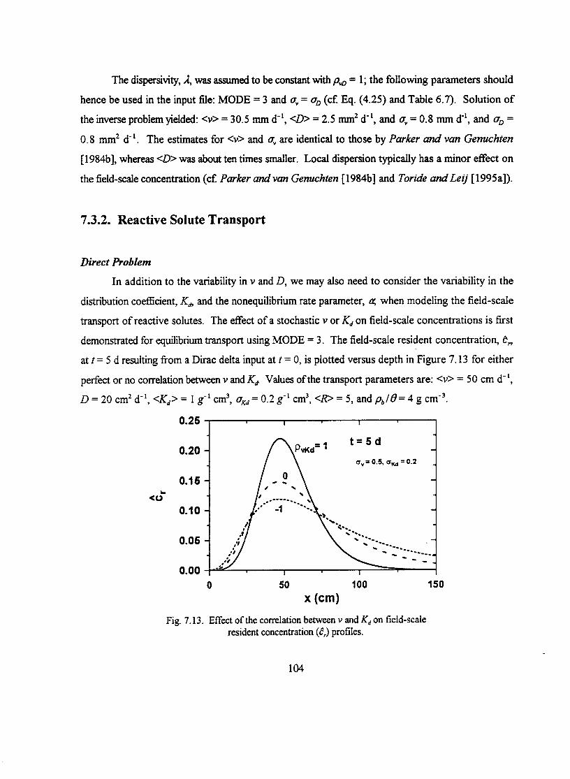
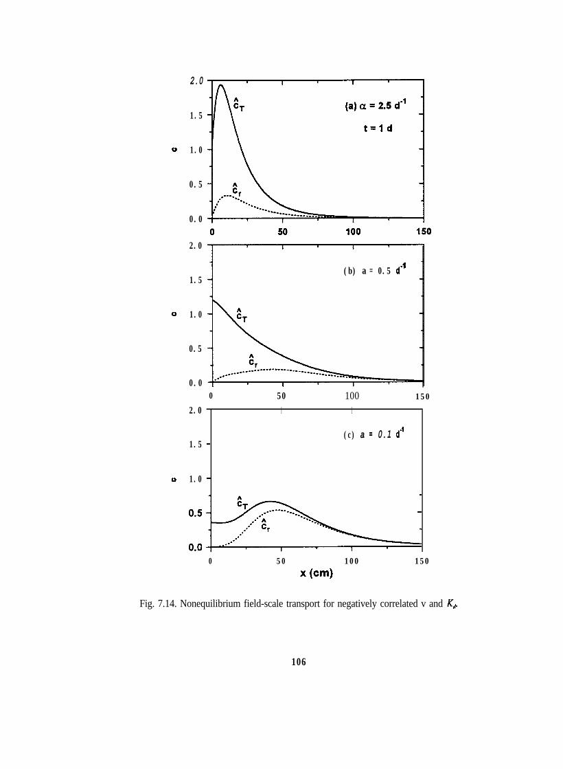
0

0

0

2.0

1.5

1.0

0.5

0.0

2.0

1.5

1.0

0.5

0.0

(b) a = 0.5 d-'

0 50 100 150

2.0 I I

(c) a = 0.1 d-'1.5 -

1.0 -

0 50 100 150

x(cm)

Fig. 7.14. Nonequilibrium field-scale transport for negatively correlated v and K,+

106

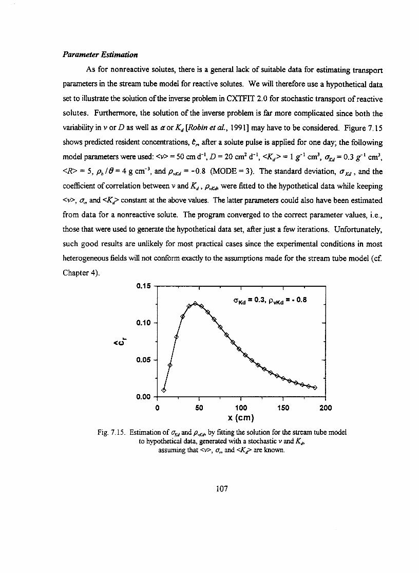
8. SUMMARY AND CONCLUSIONS

The CXTFIT 2.0 program provides a convenient way of solving direct and inverse problems

for one-dimensional solute transport during steady water flow. Both equilibrium and two-site/two-

region type nonequilibrium transport models can be implemented - the transport equation contains

terms for convection, dispersion, linear adsorption, zero-order production, and first-order decay.

Analytical solutions for deterministic transport were given for a large number of boundary, initial, and

production value problems. CXTFIT 2.0 also includes a stochastic transport model that views the

field as an assembly of deterministic flow and transport paths; these are referred to as stream tubes

for one-dimensional flow and transport. Transport in each stream tube is modeled deterministically

with the convection-dispersion equation using as random parameters v and either D, K,+ or a. The

random parameters are described with a bivariate lognormal probability density function. Solute

concentrations across the field, in either the resident or flux-averaged mode, were obtained by

averaging the concentrations of individual stream tubes.

Various transport parameters in the deterministic and stochastic transport models can be

estimated by CXTFIT 2.0 by fitting the pertinent analytical solution to solute (tracer) concentrations

obtained in the laboratory or field. As discussed in Chapter 5, the estimation procedure uses a

nonlinear least-squares inversion method according to Marquardt [ 1963]. While the procedure has

been shown to work for many examples, users should remain cognizant of potential problems

involving convergence and parameter uniqueness. This is especially true when the stream tube model

is used for optimizing data obtained across the field. Chapter 6 contains a detailed and schematic

outline of the settings and variables for each solution of the direct or inverse problem in CXTFIT 2.0.

The use of the program is further illustrated in Chapter 7, which contains a variety examples

regarding the prediction of solute profiles and the analysis of experimental data to estimate

parameters in deterministic and stochastic solute transport models.

109

Coats, K. H., and B. D. Smith, Dead-end pore volume and dispersion in porous media, Soc. Petrol.

Eng. J., 4, 73-84, 1964.

Dagan, G., Solute transport in heterogeneous porous formations, J. Fluid Mech., 14.5, 15 l-

177, 1984.

Dagan, G., Flow and Transport in Porous Formations, Springer Verlag, Berlin, 1989.

Dagan, G., The Bresler-Dagan model of flow and transport: Recent theoretical developments, in

Water flow and solute transport in soils, edited by D. Russo and G. Dagan, Springer-Verlag,

Berlin, Heidelberg, 1993

Dagan, G., and E. Bresler, Solute dispersion in unsaturated heterogeneous soil at field scale: I.

Theory, Soil Sci. Soc. Am. J., 43, 461-467, 1979.

Dagan, G., and V. Cvetkovic, Spatial moments of a kinetically sorbing solute plume in a

heterogeneous aquifer, Water Resow. Res., 29,4053-406 1, 1993.

Danckwerts, P. V., Continuous flow systems, Chem. Eng. Sci., 2, 1-13, 1953.

de Marsily, G., Quantitative Hydrogeology, Academic Press, San Diego, 1986.

De Smedt, F., and P. J. Wierenga, A generalized solution for solute flow in soils with mobile and

immobile water, Water Resour. Res., 15, 1137-l 141, 1979.

Destouni, G., and V. Cvetkovic, Field scale mass arrival of sorptive solute into the groundwater,

Water Resour. Res., 27, 13151325, 1991.

Farlow, S. J., Partial Differential Equations for Scientists and Engineers, John Wiley & Sons, New

York 1982.

Goldstein S., On the mathematics of exchange processes in fixed columns. I. Mathematical solutions

and asymptotic expansions, Proc. Roy. Soc. London., 219, 151-185, 1953.

Jury, W. A, Simulation of solute transport using a transfer function model, Water Resour. Res., 18,

363-368, 1982.

Jury, W. A., and H. Fhihler, Transport of chemicals through soils: Mechanism, model, and field

applications, Advances in Agronomy, 47, 14 l-20 1, 1992.

Jury, W. A., and K. Roth., Transfer Functions and Solute Movement through Soils: Theory and

Applications, Birkhauser, Basel, Switzerland, 1990.

112

Jury, W. A., L. H. Stolzy, and P. Shouse, A field test of a transfer function model for predicting

solute transport, Wafer Resour. Res., 18, 369-375, 1982.

Jury, W. A, and D. R Scotter, A unified approach to

Sci. Soc. Am. J., 58., 1327-1336, 1994.

Kabala, Z. J., and G. Sposito, A stochastic model

stochastic-convective transport problems, Soil

of reactive solute transport with time-varying

velocity in a heterogeneous aquifer, Water Resow. Res., 27, 341-350, 1991.

Kool, J. B., and J. C. Parker, Analysis of the inverse problem for transient unsaturated flow, Water

Resow. Res., 24, 817-830, 1988.

Kreft, A., and A. Zuber, On the physical meaning of the dispersion equation and its solutions for

different initial and boundary conditions, Chem. Eng. Sci., 33, 1471-1480, 1978.

Leij, F. J., N. Toride, and M. Th. van Genuchten, Analytical solutions for non-equilibrium solute

transport in three-dimensional porous media, J. Hydrol., 151, 193-228, 1993.

Lindstrom, F. T., Pulsed dispersion of trace chemical concentration in saturated sorbing porous

medium, Water Resow. Res., 12,229-238, 1976.

Lindstrom, F. T., and L. Boersma, Analytical solutions for convective-dispersive transport in

confined aquifers with diierent initial and boundary conditions. Water Resow. Res., 25, 241-

255, 1989.

Lindstrom, F. T., and M. N. L. Narasimhan, Mathematical theory of a kinetic model for dispersion

of previously distributed chemicals in a sorbing porous medium, SIAM J. Appl. Math., 24,

496-5 10, 1973.

Lindstrom, F. T., and W. M. Stone, On the start up or initial phase of linear mass transport of

chemicals in a water saturated sorbing porous medium: l., SIAM J. Appl. Math., 26, 578-

591, 1974.

Mailants, D., M. Vanclooster, M. Meddahi, and J. Feyen, Estimating solute transport parameters on

undisturbed soil using time domain reflectometry, J. Cont. Hydrol., 17, 91-109, 1994.

Marquardt, D. W., An algorithm for least-squares estimation of nonlinear parameters, J. Soc. Ind.

Appl. Math., II, 431-441, 1963.

Meeter, D. A, Non-linear least-squares (Gaushaus), Univ. of Wisconsin Computing Center, Program

Revised 1966.

113

Moyer, J. R., R. J. Haque, and C. E. McKone, The effect of adsorbents on the rate of degradation

of herbicides incubated with soil, Soil Biol. Biochem., 4, 307-3 11, 1972.

Nielsen, D. R, M. Th. van Genuchten, and Biggar, J. W., Water flow and solute transport processes

in the unsaturated zone, Water Resour. Res., 22, 89S-108S, 1986.

Nkedi-Kizza, P., J. W. Biggar, H. M. Selim, M. Th. van Genuchten, P. J. Wierenga, J. M. Davidson,

and D. R Nielsen, On the equivalence of two conceptual models for describing ion exchange

during transport through an aggregated oxisol, Water Resow. Res., 20, 1123-l 130, 1984,

Olver, F. W. J., Bessel functions of integer order, in Abramowitz, M. and I. A. Stegun, Handbook

of Mathematical Functions, Dover Publishing Co., New York, 355-433, 1965.

Ogram, A V., R E. Jessup, L.T. Ou, and P. S. C. Rao, Effects of sorption on biological degradation

rates of (2,4-dichlorophenoxy) acetic acid in soil, Appl. Environ. Microbiol., 49, 582-587,

1985.

Parker, J.C., and M. Th. van Genuchten, Flux-averaged and volume-averaged concentrations in

continuum approaches to solute transport, Water Resow. Rex, 20, 866-872, 1984a.

Parker, J. C., and M. Th. van Genuchten., Determining transport parameters from laboratory and field

tracer experiments, Bull. 84-3, Va. Agric. Exp. St., Blacksburg, 1984b.

Parker, J.C., and A. J. Valocchi, Constraints on the validity of equilibrium and first-order kinetic

transport models in structured soils, Water Resow. Res., 22, 399-407, 1986.

Parlange, J. -Y., J. L. Starr, M. Th. van Genuchten, D. A. Barry, and J. C. Parker, Exit condition for

miscible displacement experiments, Soil Sci., 153, 165- 17 1,1992.

Press, W.H., B.P. Flannery, S.A. Teukolsky, and W.T. Vetterling, Numerical Recipes: The Art of

Scientific Computing, 2nd ed., Cambridge University Press, New York, 1992.

Rao, P. S. C., D. E. Rolston, R. E. Jessup, and J. M. Davidson, Solute transport in aggregated

porous media. Theoretical and experimental evaluation, Soil Sci. Soc. Am. J., 44, 1139-

1146, 1980.

Robin M. J. L., E. A Sudicky, R W. Gillham, and R. G. Kachanoski, Spatial variability of Strontium

distribution coefficients and their correlation with hydraulic conductivity in the Canadian

forces base Borden aquifer, Water Resour. Res., 27,2619-2632, 1991.

114

Selim, H. M., J. M. Davidson, and R. S. Mansell, Evaluation of a two-site adsorption-desorption

model for describing solute transport in soils, In Proc. Summer Computer Simulation Conf.,

Washington, D.C., 1976.

Spiegel, M. R., Schaum’s outline of theory and problems of probability and statistics, Schaum’s

outline series, McGraw-Hill, New York, 1992.

Sposito G., and D. A Barry, On the Dagan model of solute transport in groundwater: Foundational

aspects, Water Resow. Res., 23, 1867-1875, 1987.

Sudicky, E. A, A natural gradient experiment on solute transport in a sand aquifer: Spatial variability

of hydraulic conductivity and its role in the dispersion process. Water Resour.. Res., 22,

2069-2082, 1986.

Toride, N., and F. J. Leij, Stochastic stream tube model for field-scale solute transport: I. Theory,

Soil Sci. Soc. Am. J., 1995a. (Submitted)

Toride, N., and F. J. Leij, Stochastic stream tube model for field-scale solute transport: II.

Applications, Soil Sci. Soc. Am. J., 1995b. (Submitted)

Toride, N., F. J. Leij, and M. Th. van Genuchten, A comprehensive set of analytical solutions for

nonequilibrium solute transport with first-order decay and zero-order production, Water

Resour. Res., 29, 2167-2182, 1993a.

Toride, N., F. J. Leij, and M. Th. van Genuchten, Flux-averaged concentrations for transport in soils

having nonuniform initial solute distributions, Soil Sci. Soc. Am., 57, 1406- 1409, 1993b.

van der Zee, S. E. A. T. M., and W. H. van Riemsdijk, Transport of phosphate in a heterogeneous

field, Transport Porous Media, I, 339-359, 1986.

van der Zee, S. E. A. T. M., and W. H. van Riemsdijk, Transport of reactive solute in spatially

variable soil systems, Water Resour. Res., 23,2059-2069, 1987.

van Genuchten, M. Th., Mass transfer studies in sorbing porous media, Ph.D thesis, New Mexico

State Univ., Las Cruces, 1974.

van Genuchten, M. Th., Analytical soiutions for chemical transport with simultaneous adsorption,

zero-order production and first-order decay, J. Hydrol., 49, 213-233, 1981a.

van Genuchten, M. Th, Non-equilibrium transport parameters from miscible displacement

experiments, Res. Rep. No. 119, U. S. Salinity Lab., USDA, ARS, Riverside, CA, 198 lb.

115

van Genuchten, M. Th., and W. J. Alves, Analytical solutions of the one-dimensional convective-

dispersive solute transport equation, Tech. Bull. U. S. Dep. Agri., 1661, 1982.

van Genuchten, M. Th., and J. C. Parker, Boundary conditions for displacement experiments through

short laboratory soil columns, Soil Sci. Soc. Am. J., 48, 703-708, 1984.

van Genuchten, M. Th., and J. C. Parker, Reply to “Comments on ‘Boundary conditions for

displacement experiments through short laboratory soil columns’,” Soil Sci. Soc. Am. J., 58,

991-993, 1994.

van Genuchten, M. Th., and R J. Wagenet, Two-site/two-region models for pesticide transport and

degradation: theoretical development and analytical solutions, Soil Sci. Soc. Am. J., 53, 1303-

13 10, 1989.

van Genuchten, M. Th., and P. J. Wierenga, Mass transfer studies in sorbing porous media, I,

Analytical solutions, Soil Sci. Soc. Am. J., 40,473-48 1, 1976.

Weber, J. B., and H. D. Cole, Microbial decomposition of diquat adsorbed on montmorillonite and

kaolinite clays, J. Agric. Food Chem., 16, 475-478, 1968.

Wehner, J. F., and R. H. Wilhelm, Boundary conditions of flow reactor, Chem. Eng. Sci., 6, 89-93,

1956.

116

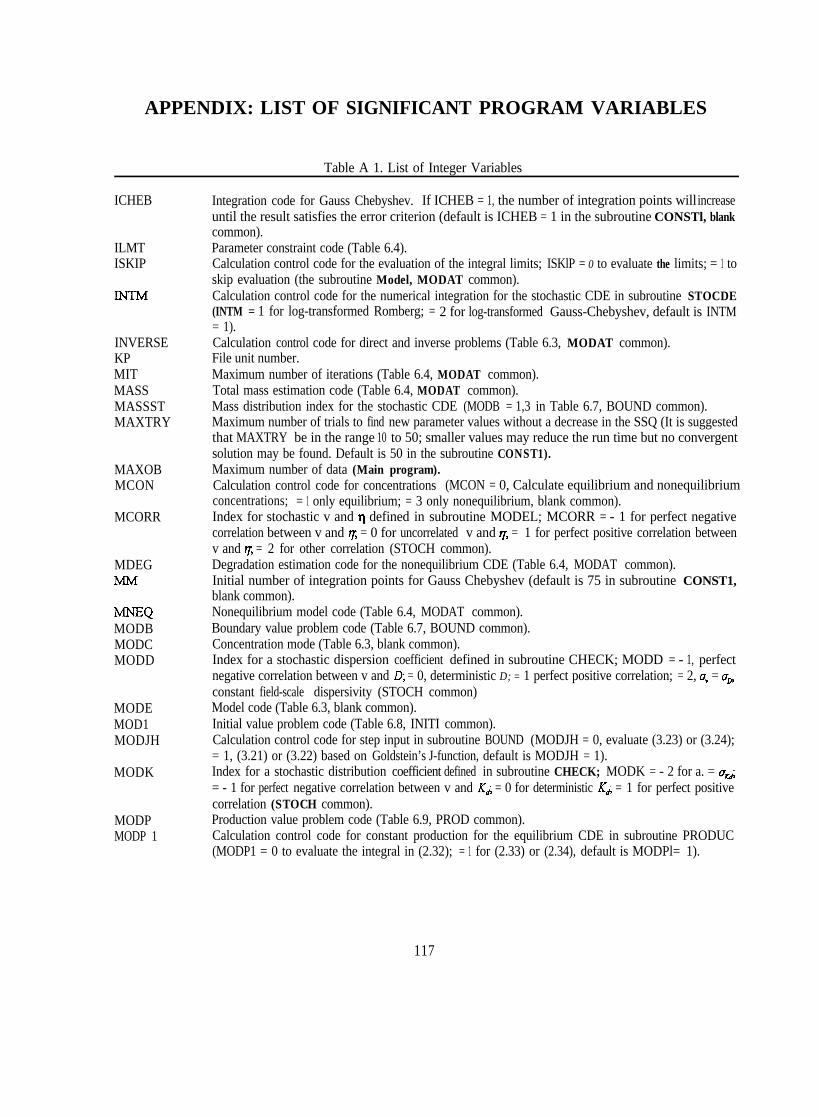
APPENDIX: LIST OF SIGNIFICANT PROGRAM VARIABLES

Table A 1. List of Integer Variables

ICHEB

ILMTISKIP

INVERSEKPMITMASSMASSSTMAXTRY

MAXOBMCON

MCORR

MDEG

MNEQMODBMODCMODD

MODEMOD1MODJH

MODK

MODPMODP 1

Integration code for Gauss Chebyshev. If ICHEB = 1, the number of integration points will increaseuntil the result satisfies the error criterion (default is ICHEB = 1 in the subroutine CONSTl, blankcommon).Parameter constraint code (Table 6.4).Calculation control code for the evaluation of the integral limits; ISKlP = 0 to evaluate the limits; = 1 toskip evaluation (the subroutine Model, MODAT common).Calculation control code for the numerical integration for the stochastic CDE in subroutine STOCDE(INTM = 1 for log-transformed Romberg; = 2 for log-transformed Gauss-Chebyshev, default is INTM= 1).Calculation control code for direct and inverse problems (Table 6.3, MODAT common).File unit number.Maximum number of iterations (Table 6.4, MODAT common).Total mass estimation code (Table 6.4, MODAT common).Mass distribution index for the stochastic CDE (MODB = 1,3 in Table 6.7, BOUND common).Maximum number of trials to find new parameter values without a decrease in the SSQ (It is suggestedthat MAXTRY be in the range 10 to 50; smaller values may reduce the run time but no convergentsolution may be found. Default is 50 in the subroutine CONST1).Maximum number of data (Main program).Calculation control code for concentrations (MCON = 0, Calculate equilibrium and nonequilibriumconcentrations; = 1 only equilibrium; = 3 only nonequilibrium, blank common).Index for stochastic v and n defined in subroutine MODEL; MCORR = - 1 for perfect negativecorrelation between v and rl; = 0 for uncorrelated v and rl; = 1 for perfect positive correlation betweenv and r7; = 2 for other correlation (STOCH common).Degradation estimation code for the nonequilibrium CDE (Table 6.4, MODAT common).Initial number of integration points for Gauss Chebyshev (default is 75 in subroutine CONST1,blank common).Nonequilibrium model code (Table 6.4, MODAT common).Boundary value problem code (Table 6.7, BOUND common).Concentration mode (Table 6.3, blank common).Index for a stochastic dispersion coefficient defined in subroutine CHECK; MODD = - 1, perfectnegative correlation between v and 0; = 0, deterministic D; = 1 perfect positive correlation; = 2, a, = o,constant field-scale dispersivity (STOCH common)Model code (Table 6.3, blank common).Initial value problem code (Table 6.8, INITI common).Calculation control code for step input in subroutine BOUND (MODJH = 0, evaluate (3.23) or (3.24);= 1, (3.21) or (3.22) based on Goldstein’s J-function, default is MODJH = 1).Index for a stochastic distribution coefficient defined in subroutine CHECK; MODK = - 2 for a. = a~= - 1 for perfect negative correlation between v and K& = 0 for deterministic &,; = 1 for perfect positivecorrelation (STOCH common).Production value problem code (Table 6.9, PROD common).Calculation control code for constant production for the equilibrium CDE in subroutine PRODUC(MODP1 = 0 to evaluate the integral in (2.32); = 1 for (2.33) or (2.34), default is MODPl= 1).

117

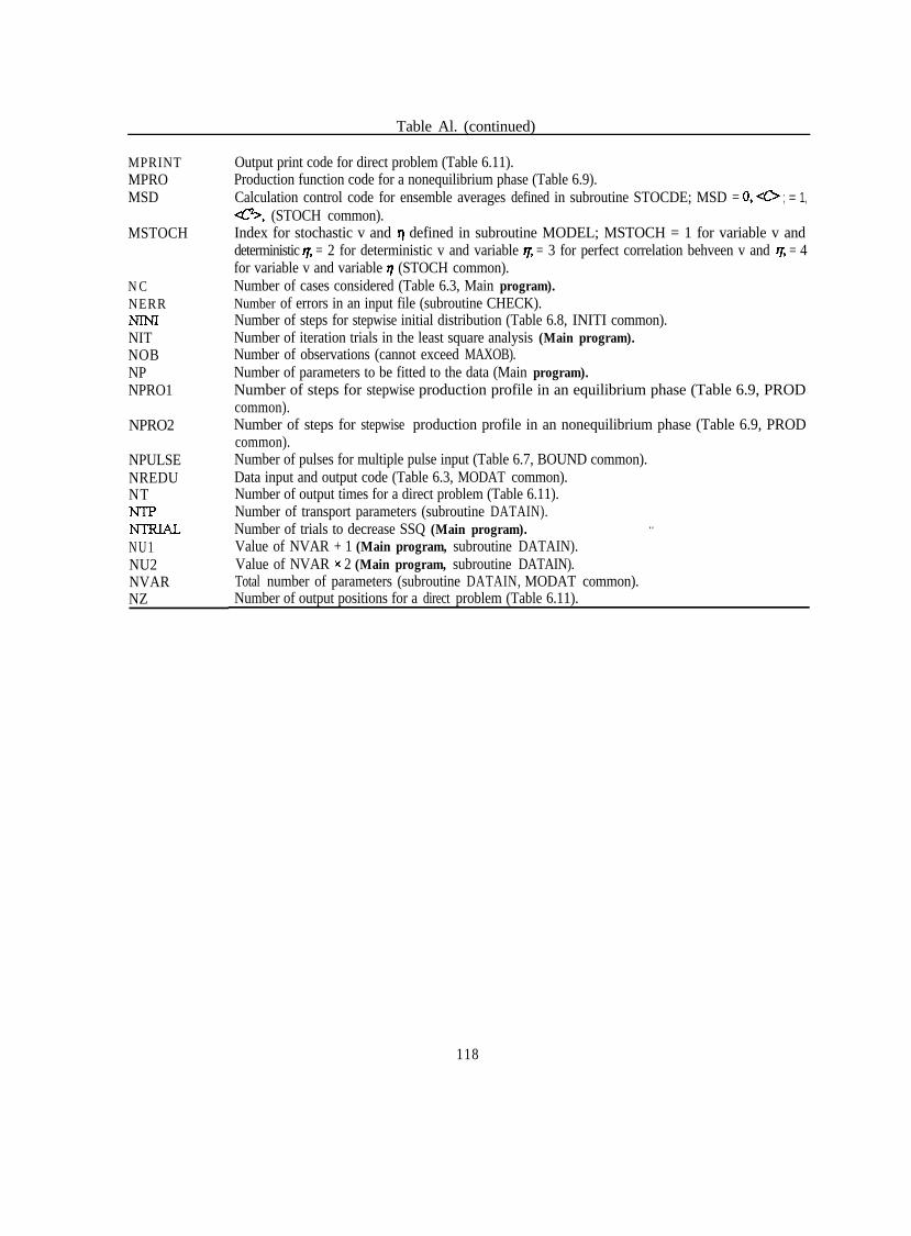
Table Al. (continued)

MPRINTMPROMSD

MSTOCH

NCNERR

NITNOBNPNPRO1

NPRO2

NPULSENREDUNT

NU1NU2NVARNZ

Output print code for direct problem (Table 6.11).Production function code for a nonequilibrium phase (Table 6.9).Calculation control code for ensemble averages defined in subroutine STOCDE; MSD = 0,9;, ; = 1,6, (STOCH common).Index for stochastic v and n defined in subroutine MODEL; MSTOCH = 1 for variable v anddeterministic r~. = 2 for deterministic v and variable r~, = 3 for perfect correlation behveen v and TT, = 4for variable v and variable 7 (STOCH common).Number of cases considered (Table 6.3, Main program).Number of errors in an input file (subroutine CHECK).Number of steps for stepwise initial distribution (Table 6.8, INITI common).Number of iteration trials in the least square analysis (Main program).Number of observations (cannot exceed MAXOB).Number of parameters to be fitted to the data (Main program).Number of steps for stepwise production profile in an equilibrium phase (Table 6.9, PRODcommon).Number of steps for stepwise production profile in an nonequilibrium phase (Table 6.9, PRODcommon).Number of pulses for multiple pulse input (Table 6.7, BOUND common).Data input and output code (Table 6.3, MODAT common).Number of output times for a direct problem (Table 6.11).Number of transport parameters (subroutine DATAIN).Number of trials to decrease SSQ (Main program). . .

Value of NVAR + 1 (Main program, subroutine DATAIN).Value of NVAR x 2 (Main program, subroutine DATAIN).Total number of parameters (subroutine DATAIN, MODAT common).Number of output positions for a direct problem (Table 6.11).

118

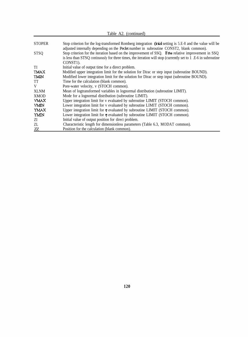
Table A2. (continued)

STOPER

STSQ

TI

TTVXLNMXMOD

ZIZLZZ

Stop criterion for the log-transformed Romberg integration (inial setting is 5.E-8 and the value will beadjusted internally depending on the Peclet number in subroutine CONST2, blank common).Stop criterion for the iteration based on the improvement of SSQ. If the relative improvement in SSQis less than STSQ continuously for three times, the iteration will stop (currently set to 1 .E-6 in subroutineCONST1).Initial value of output time for a direct problem.Modified upper integration limit for the solution for Dirac or step input (subroutine BOUND).Modified lower integration limit for the solution for Dirac or step input (subroutine BOUND).Time for the calculation (blank common).Pore-water velocity, v (STOCH common).Mean of logtransformed variables in lognormal distribution (subroutine LIMIT).Mode for a lognormal distribution (subroutine LIMIT).Upper integration limit for v evaluated by subroutine LIMIT (STOCH common).Lower integration limit for v evaluated by subroutine LIMIT (STOCH common).Upper integration limit for 7 evaluated by subroutine LIMIT (STOCH common).Lower integration limit for 11 evaluated by subroutine LIMIT (STOCH common).Initial value of output position for direct problem.Characteristic length for dimensionless parameters (Table 6.3, MODAT common).Position for the calculation (blank common).

120

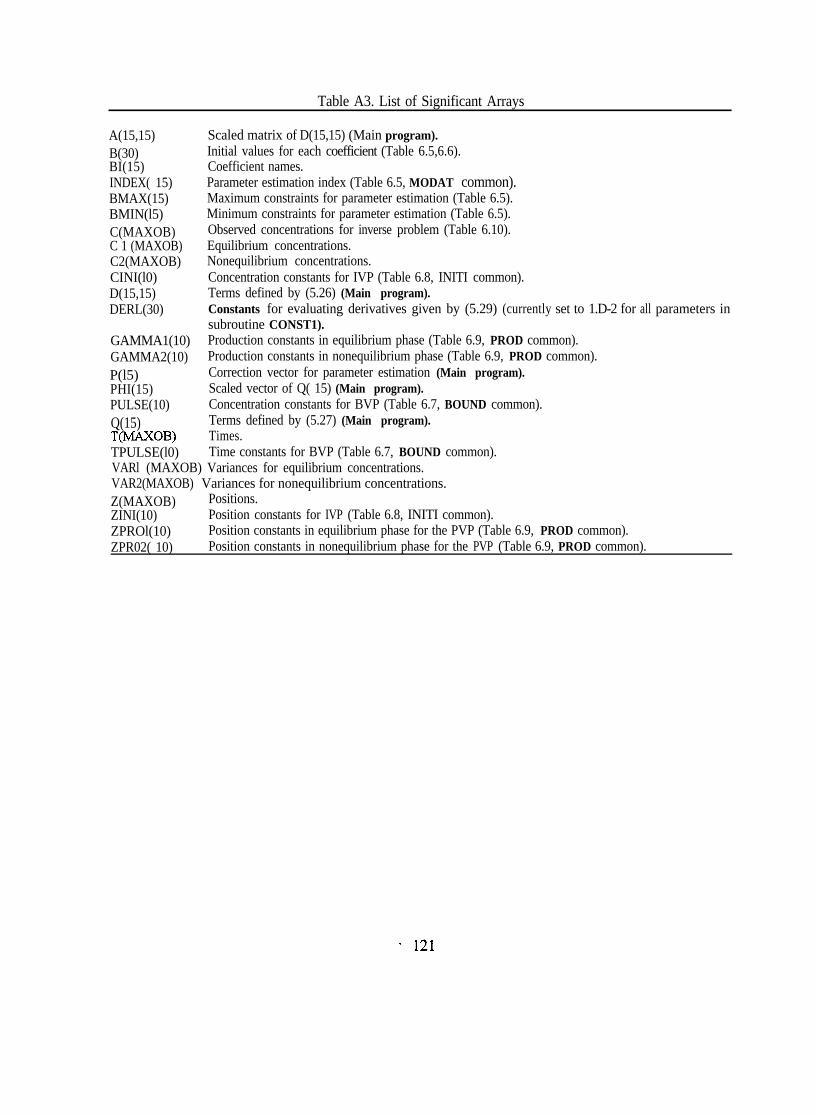
Table A3. List of Significant Arrays

A(15,15)B(30)BI(15)INDEX( 15)BMAX(15)BMIN(l5)C(MAXOB)C 1 (MAXOB)C2(MAXOB)CINI(l0)D(15,15)DERL(30)

GAMMA1(10)GAMMA2(10)P(l5)PHI(15)PULSE(10)Q(15)T(MAXOB)TPULSE(l0)

Scaled matrix of D(15,15) (Main program).Initial values for each coefficient (Table 6.5,6.6).Coefficient names.Parameter estimation index (Table 6.5, MODAT common).Maximum constraints for parameter estimation (Table 6.5).Minimum constraints for parameter estimation (Table 6.5).Observed concentrations for inverse problem (Table 6.10).Equilibrium concentrations.Nonequilibrium concentrations.Concentration constants for IVP (Table 6.8, INITI common).Terms defined by (5.26) (Main program).Constants for evaluating derivatives given by (5.29) (currently set to 1.D-2 for all parameters insubroutine CONST1).Production constants in equilibrium phase (Table 6.9, PROD common).Production constants in nonequilibrium phase (Table 6.9, PROD common).Correction vector for parameter estimation (Main program).Scaled vector of Q( 15) (Main program).Concentration constants for BVP (Table 6.7, BOUND common).Terms defined by (5.27) (Main program).Times.Time constants for BVP (Table 6.7, BOUND common).

VARl (MAXOB) Variances for equilibrium concentrations.VAR2(MAXOB) Variances for nonequilibrium concentrations.Z(MAXOB) Positions.ZINI(10) Position constants for IVP (Table 6.8, INITI common).ZPROl(10) Position constants in equilibrium phase for the PVP (Table 6.9, PROD common).ZPR02( 10) Position constants in nonequilibrium phase for the PVP (Table 6.9, PROD common).