1

The Curse of Knowledge:

When and Why Risk Parity Beats Tangency

Gregg S. Fisher, Philip Z. Maymin, Zakhar G. Maymin*

*contact author: Zak Maymin, Gerstein Fisher Research Center, zmaymin@gersteinfisher.com

Abstract

We formulate and prove several novel optimal properties of risk parity portfolios. We present

and analyze closed form solutions for the exact condition between the realized and the assumed

future parameters under which the risk parity portfolio, formed by ignoring historical average

returns, beats the tangency portfolio formed in the standard mean-variance framework. We show

under general conditions that the probability of risk parity beating tangency is more than 50

percent. We also prove that risk parity is optimal in the maximin sense: under some natural

assumptions, it will do better than any other portfolio construction method under the worst

possible combination of true expected returns. We prove the maximin properties of risk parity

portfolio under two scenarios. One such scenario assumes that all assets‟ future Sharpe ratios are

greater than some positive unknown constant and all correlations are less than another unknown

constant. Another scenario only assumes that the sum of all assets‟ future Sharpe ratio is greater

than some unknown constant. In each case, we provide explicit formulas and show that risk

parity is the unique maximin portfolio. Finally, we empirically examine historical performance

for the two main asset classes and find conformance with our theoretical results. In short,

ignoring the knowledge of past average returns to focus more deeply on risk allocation typically

leads to better performance.

2

1. Introduction

One of the most important problems a portfolio manager faces is finding the right weights for his

portfolio‟s assets. A major theoretical development for the solution to this problem was made by

Arthur D. Roy (1952). He answered the following question: if we know the first two moments

of returns, namely their expected returns and their covariance matrix, what asset weights would

maximize the mean-volatility ratio of the portfolio? We will call such portfolios tangency

portfolios because the line drawn from the risk free rate will have the highest Sharpe ratio, and

be tangent to, these portfolios.i

Portfolio managers have long realized that there was one major problem with the tangency

portfolio: the methodology required the knowledge of future first and second moments of asset

returns, and it is extremely difficult to estimate those, especially the first moments. Merton

(1980) is the classic paper showing that estimating expected returns requires a longer time period

while estimating variance requires finer observations of returns.

Even worse, with the accumulated knowledge, it became clear that in some important cases, the

weights proposed by the tangency approach were difficult to reconcile with the intuition and

experience of portfolio managers. Even Markowitz himself didn‟t follow this methodology when

constructing his own portfolio. According to Zweig (2009), he simply invested 50/50 in stocks

and bonds. Further, the tangency weights are fragile to the assumptions and can change wildly

(Britten-Jones 1999).

Risk parity (RP) is an alternative portfolio construction approach that allocates capital to each

asset inversely proportional to its future expected volatility. While it appears to take no account

3

of expected returns, it subtly does: it requires its assets to have a positive expected return;

otherwise a short position with the same volatility would be preferred.

Risk parity has tended to outperform tangency historically and several explanations for its

success have been advanced. Chaves, Hsu, Li, and Shakernia (2011) among others compared risk

parity with other more standard methods. Asl and Etula (2012) discuss risk parity and similar

portfolio construction strategies from the perspective of robust optimization; building on Scherer

(2007), Meucci (2007), and Ceria and Stubbs (2006), they consider the standard errors of the

expected return estimations as the sole source of uncertainty, and show that in such cases,

portfolios similar to but different from risk parity would be optimal. By contrast, we consider

two more general cases that depend only on mild conditions on future asset Sharpe ratios to show

that pure risk parity would be uniquely optimal.

Asness, Frazzini, and Pedersen (2012) show that leverage aversion can lead to excess returns to a

risk parity portfolio, and they document RP‟s historical and sustained outperformance. Here, we

show that even if leverage aversion did not apply, risk parity would still beat tangency on

average, under the precise conditions we provide.

Risk parity versus tangency can be thought of as a battleground in the larger war between

seemingly ad-hoc heuristics-based approaches and traditional optimization approaches to finance

in general and portfolio management specifically. By exploring this arena in detail, we aim to

shed light on the larger question.

The term “heuristics” generally means “rule of thumb.” It is used in behavioral sciences in a

predominately pejorative sense when compared to unattainable perfect rationality. However, in

computational discussions, heuristics are simple but crucial algorithms that substantially improve

4

performance. In the context of boundedly rational investor behavior, Gigerenzer (2012) argues

that particular heuristics are “ecological” in the sense that they can be helpful in particular

circumstances, and are neither universally good nor universally bad. Goldstein and Gigerenzer

(2009) show that fast and frugal heuristics can make better predictions than more complex and

more knowledge-intensive rules.

In this context, we argue that risk parity, as a fast and frugal heuristic, tends to outperform the

more complex and more knowledge-intensive mean-variance approach. One candidate for the

cognitive bias preventing all investors from pursuing risk parity might be due to what Camerer,

Loewenstein, and Weber (1989) refer to as the “curse of knowledge,” a term they attribute to

Robin Hogarth, where they demonstrate economic and market transactions in which agents with

more knowledge are unable to ignore that knowledge, even when doing so would be to their

advantage.

Of course, risk parity‟s outperformance is not ubiquitous. Indeed, during 2012, because of the

lackluster performance of bonds, tangency actually beat risk parity. That makes the main

questions of this paper especially timely: what is the condition on future parameters that makes

one approach preferable to the other? Are there any conditions under which risk parity approach

is optimal in some sense? Can we estimate the probability that risk parity will outperform? This

paper addresses all these questions and more in a novel and general theoretical framework, with

supporting empirical results.

5

2. Tangency Portfolio

The tangency portfolio has the highest Sharpe ratio for assets having random excess returns:

( )

such that

( ) and ( )

where

( ) and { }

We write , the transpose of to emphasize that we normally define new vectors as column

vectors. So is a column vector and is a row vector.

The tangency portfolio with weights ( ) maximizes the Sharpe ratio:

√

Instead of the usual solution of this optimization problem using a Lagrange multiplier, we will

solve it using a linear algebraic and geometric framework that will be useful for us in later

sections.

Because is a positive-definite symmetric matrix, by the spectral decomposition theorem it can

be written as:

6

where is an orthonormal matrix, . The columns of are eigenvectors of length 1 of

and is the diagonal matrix of the corresponding positive eigenvalues of .

Let us introduce new variables ( ) as the coordinates of our vector of

portfolio weights in the new orthonormal basis given by the eigenvectors of .

By the definition of and . Therefore:

√

√

Define

. The diagonal matrix

is well-defined because is positive definite. So

. It is easy to see that

, and therefore

, and:

√

√

The optimum weights stay optimal if we multiply them by any positive constant. So we can

assume for the moment that lies on a unit sphere, . Then to achieve the maximum in

the dot product of two vectors in the numerator of the last expression for , must be parallel

to

, where is a constant found from the condition that the length of

is 1, namely (

) . So

√

Then the optimal Sharpe ratio SR* is:

7

( )

√ √

And the optimal weights are proportional to:

If we impose the normalizing condition , where is a column vector of ones, then the

optimal weights are:

( )

3. Risk Parity and Equal Risk Contribution

The Risk Parity (RP) weights ( ) are by definition inversely proportional to the

asset volatilities:

(

)

√

Taking into account the normalizing constraint ∑ , we have:

∑

And its Sharpe ratio is:

( )

√( )

8

Let us define the Equal Risk Contribution (ERC) portfolio. The volatility of a portfolio with

weights ( ) is:

( ) √ √∑

∑ ∑

Define the risk contribution of asset as:

( ) ( )

∑

( )

Therefore the risk (volatility) of the portfolio can be presented as the sum of its asset risks:

( ) ∑ ( )

The Equal Risk Contribution portfolio is defined by requiring that all assets‟ risks are equal:

( ) ( )

Two additional constraints are usually enforced, namely, the normalizing constraint:

∑

and the no-short-selling constraint:

Note that these definitions are not universally accepted. Sometimes Equal Risk Contribution

portfolios are called Risk Parity portfolio, and what we define as the Risk Parity portfolio are

sometimes called Naïve Risk Parity portfolios.

9

Actually, it would have been more exact and more specific to call a RP portfolio a Volatility

Parity portfolio and ERC portfolio a Beta Parity portfolio. Here is the logic why (see Maillard,

Thierry and Teiletche (2010)). Denote the covariance between the th asset and the portfolio by

( ∑ ) ∑ . Then ( ) ( ). By definition, the beta of asset

with the portfolio is ( ). We know that for the ERC portfolio ( ) ( ) for

all . Therefore:

( ) ( )

∑

This is the same formula as for RP, only using betas instead of volatilities.

It is important to notice that in a very important general parameter case, the RP portfolio is the

same as the ERC portfolio: namely, Maillard, Thierry and Teiletche (2010) proved that ERC

becomes a RP portfolio when the correlations among all assets are the same. In particular, for

, the ERC portfolio is the RP portfolio. Exact formulas for the weights of ERC portfolio

are not known in the general case. Chaves, Hsu, Li, and Shakernia (2012) analyze algorithms for

computing those weights.

4. Maximin Optimality of Risk Parity

We establish two maximin properties of risk parity.

In both cases we fix a certain set of parameters and show that the minimum Sharpe ratio of the

RP portfolio on this set is greater than the minimum Sharpe ratio on the same set of any other

portfolio.

10

4.1. Each asset’s Sharpe ratio is positive and all correlations are less than one.

Let us define a set of parameters when each asset‟s Sharpe ratio is greater than some positive

constant and all correlations between different assets are less than some constant:

(

)

(

)

This parameter set describes a situation when the portfolio manager knows the asset volatilities

but does not know either the asset expected returns or the correlations between asset returns.

Yet he knows something. He chose assets with enough care that he is reasonably certain that the

worst Sharpe ratio of any asset is still positive. In other words, all he knows about chosen assets

is that the expected return of each should be positive, but he doesn‟t necessarily know which of

them would perform better than others. Further, he also believes that different assets are indeed

different, with correlations less than one.

Let‟s consider the normalized portfolio with no short sales:

∑

Then the Sharpe ratio of this portfolio is:

√

Introducing new variables ( ), we can rewrite this as:

11

√

Obviously the Sharpe ratio achieves its smallest possible value when the numerator is as small as

possible and the denominator is as large as possible:

√

Where is a correlation matrix with all correlations equal to .

To finish our proof we need the following statement: if the Sharpe ratios of all assets are equal

and their correlations are all equal, then the risk parity portfolio is the tangency portfolio.

Maillard, Thierry and Teiletche (2010) proved this statement. A different proof was offered by

Kaya and Lee (2012). We‟ll give here yet another, simpler proof.

We know that the weights of the tangency portfolio are proportional to . All we need to

show is that this is a product of a constant times 1. If correlations are equal, row sums of are

equal,

for some constant . Thus , which proves the result. Analysis of the proof shows that

the risk parity is the only maximin portfolio.

4.2. The sum of all assets’ Sharpe ratios is positive

Let us define a set of parameters when the sum of the Sharpe ratios of all of the assets is greater

than some positive constant.

12

*

∑

+

This parameter set describes a situation when the portfolio manager is reasonably certain that in

the worst case the total sum of all assets‟ Sharpe ratios cannot be less than some positive

constant. In this case, any particular asset may even have a negative Sharpe ratio, so long as the

simple total (or, equivalently, average) across all assets is still positive.

Let us again consider a normalized portfolio with no short sales:

∑

This portfolio‟s Sharpe ratio is:

√

In the worst case we have:

( )

√

We need to find maximum in of the following function:

( )

( )

√

The for which this function achieves its maximum is the same vector on which the following

function achieves its minimum:

13

( )

(

( ) )

∑

because (

)

( )( ) . And therefore:

( )

√∑

For the risk parity portfolio weights, , , we have:

( )

√ ( )

∑

√

√∑

which finishes the proof. Analysis of the proof shows that the risk parity is the only maximin

portfolio.

5. When Risk Parity Beats Tangency by Sharpe Ratio

Say weights outperform weights for a given and if they result in a higher Sharpe ratio:

( )

√ ( )

√

where are the assets‟ future expected returns, is the assets‟ future variance matrix, and and

are portfolios weights based on the past expected returns and the past variance matrix .

Taking as the weights for the risk parity portfolio, and as the weights for the tangency

portfolio, we see that risk parity outperforms tangency if and only if:

14

(

√( )

√ )

This defines an -dimensional hyperplane for the vectors . This hyperplane passes through the

origin and is perpendicular to the vector:

(

√( )

√ )

The future returns do not depend on the future variance matrix and therefore risk parity beats

tangency in expected returns if and only if:

(

)

5.1. Case when the future variance matrix is equal to the past variance matrix

If the future variance matrix is equal to the past, then risk parity beats tangency if and only if:

(

√( )

√ )

Let us simplify the general expression for the difference in Sharpe ratios between RP and any

arbitrary portfolio, if the future variance matrix is equal to the past. We will use the fact that

and where R is the correlation matrix and is the diagonal

matrix with vector x on its diagonal. Then

. So:

( )

Let us use the Sharpe ratios instead of expected returns of assets:

15

{ } {

}

We already established that RP outperforms any portfolio with weights by Sharpe if:

(

√

√ )

If * + then the last inequality can be rewritten as:

(

√

√ )

or:

(

√

√ ) (5.1.1)

The Sharpe ratio of the tangency portfolio is (( ) ).

√

( )

√( ) ( )

√

Therefore RP beats tangency in Sharpe ratio if and only if:

(

√

√ )

(5.1.2)

16

6. Probability that Risk Parity Beats Any Other Portfolio is Greater than 50%

Assume that all future asset variances are the same as the past and all future asset correlations are

equal to a non-negative number. Assume that the directions of the assets‟ future Sharpe ratios

are drawn completely randomly from the positive hyperquadrant * +.

Then we can show that the probability that risk parity beats any other portfolio with positive

coefficients by Sharpe ratio is greater than 50%.

To begin, we rewrite the inequality in Equation (5.1.1) as:

( ) (6.1)

where

√ , ‖ ‖ and

√ ‖ ‖

√ √ .

The vector is the rotation axis of . Therefore to prove our statement it is sufficient to prove

that either: A) lie on different sides of the hyperplane defined by Equation (6.1), or B)

and lie on the same side of the hyperplane but the distance of (which is a unit vector in the

direction of the portfolio with weights ) from the hyperplane is longer than the distance of

from the same hyperplane.

Assume for all and that (we will prove this statement at the end.) Then:

( ) (6.2)

because and are unit vectors.

17

Now, let us analyze the two cases.

A) Because of Equation (6.2), for to lie on different sides of the hyperplane we must

have:

( )

which is equivalent to:

(6.3)

B) We can now assume that (6.3) doesn‟t hold:

(6.4)

The distance from a unit vector to a plane passing through the origin perpendicular to a

vector is | | | | . For our hyperplane defined by Equation (6.1), .

Therefore the distance from to the hyperplane is:

| |

because . The distance from to the hyperplane is

| |

where the last equation follows because of (6.4).

is further from the plane than if and only if:

which is obvious because and are unit vectors.

The only thing remaining to be proved is that or:

18

(6.5)

The right hand side of Equation (6.5) is equal to ( ) , where is the correlation

between any two assets, the common term in matrix . The left hand side of Equation (6.5) is the

so-called Raleigh quotient and is never greater than , the maximum eigenvector of matrix .

According to Morrison (1967, 244-245):

( )

That completes the proof.

6.1. Illustration for Uncorrelated Assets

In this case, according to Equation (5.1.2):

(

√

√ )

We can depict the result geometrically, as shown in Figure 1.

Here (

√

√ ),

‖ ‖ is a unit vector, is an arbitrary vector of the assets‟ past Sharpe

ratios from the positive quadrant, by definition, and is the angle between e and d

so that ( ) .

19

Figure 1

We assumed that the assets‟ future Sharpe ratios ( ) are randomly chosen from the

positive quadrant of a unit circle. Then the probability that risk parity beats tangency for two

assets is easily seen geometrically to be:

7. When Risk Parity Beats Tangency Empirically

Consider an investor allocating between the two main asset classes: equities and bonds. The

investor observes the monthly returns of both time series and compares three possible portfolios:

the risk parity portfolio that invests inversely proportional to each asset‟s realized volatility, the

tangency portfolio that invests in the portfolio that would have had the highest ex ante realized

Sharpe ratio, and the fixed portfolio that invests 60 percent in stocks and 40 percent in bonds.

20

How would the investor have performed historically under each of those three possibilities? We

take the monthly total returns of the S&P 500 index from Bloomberg and the monthly total

returns of the Barclays Capital US Aggregate Bond Index from Dimensional Fund

Advisors (DFA) Returns 2.0 software, from February 1988 through October 2012.

Figure 2 shows the 24-month rolling Sharpe ratios of these three portfolios, formed using the

returns from the previous 24 month period, and held for the subsequent 24 month period. Risk

parity outperformed both other portfolios, averaging a 0.99 Sharpe ratio. The tangency portfolio

was the worst, averaging a 0.48 Sharpe ratio. The fixed 60/40 portfolio averaged a 0.68 Sharpe

ratio.

Figure 2

The weights for the tangency portfolio fluctuate wildly. Figure 3 shows a paired histogram

comparing the distributions of the risk parity and tangency portfolio‟s equity weighting (the

fixed 60/40 portfolio was always a constant 0.60). The risk parity equity weighting was always

between 12.7 percent and 37.9 percent while the tangency portfolio ranged from -8,957 percent

21

to 2,644 percent; the figure shows the clipped distribution with all weights below -1 or above +1

reflected in those final bars.

Figure 3

To test the implications from our theoretical framework, we can examine the sensitivity of the

performance of the risk parity and tangency portfolios to the performance of the underlying

assets. Figure 4 plots the Sharpe ratio of each of the two portfolios separately, as well as the

excess Sharpe ratio of the risk parity portfolio over the tangency portfolio, relative to the Sharpe

ratios of the stocks and bonds separately, as well as to their sum. The best-fit regression line is

overlayed. All Sharpe ratios are computed for the same time periods, on a rolling 10-month

basis.

Consider the first column in Figure 4, showing the relation between the portfolio Sharpe ratio

and the stock Sharpe ratio during the same time period. Counter to the usual intuition that

tangency outperforms risk parity when equities outperform, we can see that empirically risk

parity performs better when stocks perform better, while the performance of the tangency

portfolio is essentially unrelated to the simultaneous performance of stocks.

22

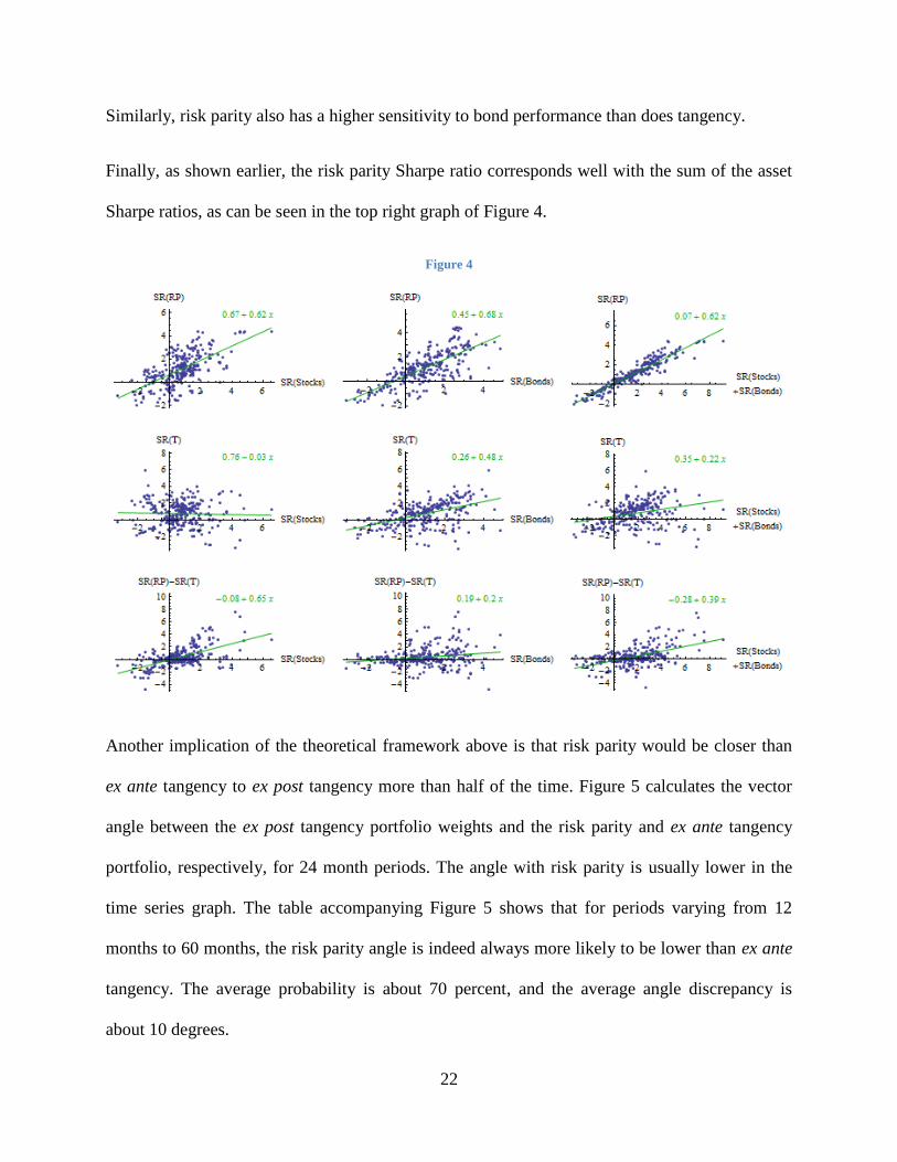
Similarly, risk parity also has a higher sensitivity to bond performance than does tangency.

Finally, as shown earlier, the risk parity Sharpe ratio corresponds well with the sum of the asset

Sharpe ratios, as can be seen in the top right graph of Figure 4.

Figure 4

Another implication of the theoretical framework above is that risk parity would be closer than

ex ante tangency to ex post tangency more than half of the time. Figure 5 calculates the vector

angle between the ex post tangency portfolio weights and the risk parity and ex ante tangency

portfolio, respectively, for 24 month periods. The angle with risk parity is usually lower in the

time series graph. The table accompanying Figure 5 shows that for periods varying from 12

months to 60 months, the risk parity angle is indeed always more likely to be lower than ex ante

tangency. The average probability is about 70 percent, and the average angle discrepancy is

about 10 degrees.

23

Figure 5

( ) ̅̅ ̅̅ ̅ ̅̅ ̅

8. Conclusion

Forming risk parity portfolios does not require as much data and as many sophisticated tools as

forming other portfolios, such as the tangency portfolio embraced by standard portfolio theory.

Yet lately it has become a prominent instrument among fund managers and a central topic among

academic researchers, due largely to its consistent outperformance.

We have described the exact parametric conditions when risk parity outperforms other portfolios,

including tangency. This research provides mathematical validation for portfolio managers

choosing risk parity under uncertainty by formulating the exact conditions of those uncertainties

and proving precise mathematical results about the superiority of risk parity portfolio under those

conditions.

24

We formulate and prove several optimal properties of risk parity portfolios including new

maximin properties under two scenarios. The maximin approach finds the portfolio that performs

the best under the worst possible future distributional parameters of the assets. One such scenario

assumes that all assets‟ future Sharpe ratios are greater than some positive unknown constant and

all correlations are less than another unknown constant. Another scenario only assumes that the

sum of all assets‟ future Sharpe ratio is greater than some unknown constant. In each case, we

provide explicit formulas and show that risk parity is the unique maximin portfolio.

We also show that for a positive constant correlation matrix, assuming that the assets‟ future

positive Sharpe ratios are chosen at random, the probability that the risk parity portfolio beats by

Sharpe ratio any other portfolio is greater than 50%. This novel theoretical result has important

practical applications. If the only thing that portfolio manager is able to predict about the future

parameters are the ratio of assets variances, then under very general conditions, he should choose

risk parity because there is a more than 50% chance that it will beat any other portfolio. Further,

we find empirical support for this prediction for a wide variety of time periods when comparing

the past several decades of domestic equity and bond returns.

We have thus shown not only when and why risk parity outperforms tangency, but also provided

a framework and direction for showing how and when a heuristic approach ignoring some

knowledge may in general beat a more traditional optimization approach utilizing all knowledge.

Future research includes adopting this approach to other areas such as risk management, dynamic

asset allocation, and derivatives valuation to provide both theoretical justification and empirical

validation that heuristics can consistently and strongly outperform, and that sometimes, too much

knowledge can be a curse, and ought to be ignored.

25

References

Asl, Farshid M., and Erkko Etula. 2012. “Advancing Strategic Asset Allocation in a Multi-Factor

World.” The Journal of Portfolio Management 39:1, 59-66.

Asness, Cliff, Andrea Frazzini, and Lasse H. Pedersen. "Leverage Aversion and Risk

Parity." Financial Analysts Journal 68.1 (2012): 47-59.

Britten-Jones, Mark, 1999. “The Sampling Error in Estimates of Mean-Variance Efficient

Portfolio Weights,” The Journal of Finance , 54:2, 655-671.

Camerer, Colin, George Loewenstein, and Martin Weber, 1989. “The Curse of Knowledge in

Economic Settings: An Experimental Analysis.” The Journal of Political Economy 97:5,

1232-1254.

Ceria, S. and R.A. Stubbs, 2006. “Incorporating Estimation Errors into Portfolio Selection:

Robust Portfolio Construction.” Axioma Research Paper No. 3.

Chaves, Denis B., Jason Hsu, Feifei Li, and Omid Shakernia, 2011. “Risk Parity Portfolio vs.

Other Asset Allocation Heuristic Portfolios.” Journal of Investing, vol. 20, no. 1

(Spring):108–118.

Chaves, Denis B., Jason Hsu, Feifei Li, and Omid Shakernia, 2012. “Efficient Algorithms for

Computing Risk Parity Portfolio Weights.” Journal of Investing, vol. 21, no. 3

(Fall):150–163.

Gigerenzer, G. Todd, Peter M., ABC Research Group. 2012. “Ecological Rationality:

Intelligence in the World.” Oxford University Press, New York.

Goldstein, Daniel G., Gigerenzer Gerd. 2009. “Fast and frugal forecasting.” International Journal

of Forecasting, 25, 760-772.

Kaya, H., and Lee, W. 2012 “Demystifying Risk Parity.” White paper, Neuberger Berman, 2012

Markowitz, Harry. 1952. “Portfolio Selection.” The Journal of Finance, vol.7, no.1, 77-91.

Maillard, Sébastien, Thierry Roncalli, and Jérôme Teiletche. 2010. “The Properties of Equally

Weighted Risk Contribution Portfolios.” Journal of Portfolio Management, vol. 36, no. 4

(Summer):60–70.

Meucci, A. 2007. “Risk and Asset Allocation.” New York: Springer.

Merton, Robert C., 1980. “On estimating the expected return on the market: An exploratory

investigation.” Journal of Financial Economics 8, 323-361.Markowitz, H., 1952.

Portfolio selection. Journal of Finance 7, 77–91.

Morrison, D. R. “Multivariate statistical methods.” New York: McGraw-Hill, 1967.

Roy, Arthur D. 1952. Safety First and the Holding of Assets. Econometrica, 20:3, 431-449.

26

Sharpe, William F. 1966. “Mutual Fund Performance.” The Journal of Business, Vol. 39, no.1

119-138.

Scherer, B. 2007. “Can Robust Portfolio Optimization Help Build Better Portfolios?” Journal of

Asset Management 7, 374-387.

Sullivan, Edward J. 2011. A.D.Roy: the forgotten father of portfolio theory. Resesarch in the

history of economic thought and methodology; 29.pp.73-82.

Zweig, Jason. 2009. “Investing Experts Urge „Do as I Say, Not as I Do‟” The Wall Street

Journal, January 3, 2009.

i We are aware that normally the optimality result is attributed to Markowitz or Sharpe. However, the founding

papers of modern portfolio theory, Markowitz (1952) and Sharpe (1966) don‟t have this result while Roy (1952)

does. See some discussion of Roy‟s forgotten contribution in Sullivan (2011). As an aside, in his paper Roy also

introduces the concept of Value at Risk. Markowitz (1952) appears to be the first to suggest evaluating portfolios by

the relationship between their expected returns and their variances and to develop the concept of efficient portfolios.