Embed Size (px)
Citation preview
THE CRIMINAL AND LABOR MARKET IMPACTS OF INCARCERATION
MICHAEL MUELLER-SMITH∗
SEPTEMBER 2014
ABSTRACT. This paper investigates the pre- and post-release impacts of incarceration on criminalbehavior, economic wellbeing and family formation using new data from Harris County, Texas. Theresearch design identifies exogenous variation in the extensive and intensive margins of incarcera-tion by leveraging the random assignment of defendants to courtrooms. I develop a new data-drivenestimation procedure to address multidimensional and non-monotonic sentencing patterns observedin my courtrooms in my data. My findings indicate that incarceration generates modest incapacita-tion effects, which are offset in the long-run by an increased likelihood of defendants reoffendingafter being released. Additional evidence finds that incarceration reduces post-release employmentand wages, increases take-up of food stamps, decreases likelihood of marriage and increases thelikelihood of divorce. Based on changes in defendant behavior alone, I estimate that a one yearprison term for marginal defendants conservatively generates between $71,000 to $81,800 in socialcosts, which would require substantial general deterrence in the population to at least be welfareneutral.
Keywords: incarceration, recidivism, labor market outcomes, family formation, monotonicity
JEL: J24, K42, J62
∗Department of Economics, Columbia University (email: [email protected]). I would like to thankCristian Pop-Eleches, Bernard Salanie and Miguel Urquiola for their advice and support. I also benefited from con-versations with Doug Almond, Sandra Black, Scott Cunningham, Keshav Dogra, Keith Finlay, Colin Hottman, JuHyun Kim, Christopher King, Wojciech Kopczuk, Ilyana Kuzmienko, Steve Levitt, John List, Jens Ludwig, MayaRossin-Slater, Aurelie Ouss, Emily Owens, Kevin Schnepel, Hyelim Son, Patrick Sun, and Lesley Turner. I wouldalso like to thank the participants in the NBER Summer Institute and Columbia Applied Microeconomics Workshopfor their comments. I am particularly indebted to the staff at the Ray Marshall Center who have generously hosted myresearch in Texas. This project would not have been possible without the approval of the Harris County District Clerk,the Harris County Sheriff’s Office the Texas Department of Criminal Justice, the Texas Department of Public Safety,the Texas Health and Human Services Commission, and the Texas Workforce Commission. Funding for this projectwas provided by the National Science Foundation (SES-1260892).
1
2 MICHAEL MUELLER-SMITH
The United States currently has the highest incarceration rate in the world (Walmsley [2009]), a
consequence of three decades of dramatic growth in the prison population since the late 1970s (Car-
son [2013]). Over this same time period governmental expenditures on police protection, judicial
and legal systems, and corrections also surged (Bureau of Justice Statistics [1980] and Kyckelhahn
[2013]). Recent estimates indicate that the annual U.S. correctional population included over 7
million adults (Glaze and Herberman [2013]), and combined federal, state and local expenditures
on justice-related programs topped $260 billion per year. Despite the reach and cost associated
with these changes to criminal justice policy, causal evidence on how this use of incarceration has
impacted the population remains scarce (see Donohue III [2009]).
To help address this gap in the literature, I investigate the impacts of incarceration using original
data from Harris County, Texas. The new data is comprised of over 2.6 million criminal court
records accounting for 1.1 million unique defendants, which I collected and processed into an em-
pirical dataset. It captures the universe of misdemeanor and felony criminal charges between 1980
and 2009 regardless of final conviction status. What makes the data especially unique is the ability
to link the court records to a variety of other sources of administrative data including state prison
and county jail data, unemployment insurance wage records, public assistance benefits, marriage
and divorce records as well as future criminal behavior using individual identifiers available in the
data. Taken together, the combined data allows me to estimate impacts on a broad range of policy-
relevant outcomes, promoting a better understanding of the potential mechanisms underpinning
the treatment effects and providing for a more complete accounting in the cost benefit analysis of
incarceration.
The research design leverages the random assignment of criminal defendants to courtrooms as
a source of exogenous variation in both the extensive and intensive margins of incarceration. The
courts are staffed by judges and prosecutors who differ in their propensity to incarcerate. As a
result, which courtroom a defendant is randomly assigned to strongly predicts whether he will be
incarcerated and for how long.1 This increasingly popular identification strategy has been used in a
1Even though parole boards may adjust some sentences ex-post, my evidence indicates that the courts exert influ-ence over actual time served.
THE CRIMINAL AND LABOR MARKET IMPACTS OF INCARCERATION 3
number of applications where judges, case workers, or other types of programs administrators are
given discretion on how to respond to a randomly assigned caseload.2
The application considered in this paper is moderately more complex than standard uses of this
research design. Sentencing takes on multiple dimensions (e.g. incarceration, fines, drug treatment,
etc.) and judges display non-monotonic tendencies (e.g. a judge may incarcerate drug offenders at
a relatively higher rate but property offenders at a relatively lower rate). Since failure to account
for these features of the data could lead to violations of the exclusion restriction and monotonicity
assumption, a new estimation procedure is developed.3 In this new approach, I first construct
instruments for each observable aspect of sentencing, not just incarceration, in order to control
for court tendencies on non-focal sentencing dimensions. I also relax the first stage equation to
allow the impact of court assignment on sentencing outcomes to flexibly respond to observed
defendant characteristics. Because this second modification can generate many instruments due to
the curse of dimensionality, the least absolute selection and shrinkage operator (LASSO) is used in
conjunction with cross validation as a data-driven tool to achieve disciplined dimension reduction
without skewing statistical testing.
My empirical findings indicate that incarceration for marginal defendants is less attractive from
a policy perspective than has been shown in prior work. I measure modest incapacitation effects
while defendants are in jail or prison: defendants are 4.1 to 4.8 percentage points less likely to
be charged with a new criminal offense while incarcerated. This benefit, however, is offset by
increases in post-release criminal behavior: each additional year that a felony defendant was incar-
cerated increases the probability of facing new charges post-release by 5.4 percentage points per
quarter. Partially driving this result is a pattern of former inmates being charged with new crime
types. In particular, I find that former inmates are especially likely to commit more property (e.g.
theft or burglary) and drug-related crimes after being released, even if these crimes were not their
original offenses.
2For studies specifically related to incarceration, see Kling [2006], Di Tella and Schargrodsky [2004], or Aizerand Doyle [2013]. For research in other fields, see Doyle [2007, 2008], Autor and Houseman [2010], Belloni et al.[2012], Munroe and Wilse-Samson [2012], Doyle et al. [2012], French and Song [2012] Maestas et al. [2013], Autoret al. [2013] and Dahl et al. [2013].
3Prior researchers have acknowledged the potential for these features to also affect their findings, but data limita-tions have generally limited their ability to address these concerns in any formal way.

4 MICHAEL MUELLER-SMITH
In contrast with prior work, I find strong evidence that incarceration has lasting negative effects
on labor market outcomes after defendants have been released. I find that each additional year of
incarceration reduces post-release employment by 3 to 6 percent points. Among felony defendants
with stable pre-charge income, only 39 percent were able to return to employment in the 5 years
after being released. While there are no discernible impacts on welfare payments, Food Stamps
take-up increases post-release providing further evidence of lasting economic hardship.
The impacts of incarceration extend beyond recidivism and labor market outcomes. Incarcer-
ation appears to negatively impact family formation and stability as measured through marriage
and divorce activity. While incarcerated, young felony defendants exhibit significantly lower rates
of marriage that is not compensated post-release indicating a net decline in marriage rather than
a temporal shift. Further supporting this conclusion, I find that divorce rates among older felons
increase post-release for each additional year of incarceration.
Using these new estimates, I reevaluate the welfare impacts of incarceration. Because I cannot
measure general deterrence effects in my research design, the cost benefit exercise is partial in
nature and only accounts for the administrative expenses, criminal behavior effects and economic
impacts associated with the defendant’s own outcomes. Using the most conservative estimates, I
find that a one year prison term for marginal defendants decreases social welfare by $71,000 to
$81,800 of which negative impacts to economic activity account for 53 to 61 percent of overall
costs. In order for this sentence to be neutral in social welfare terms, a one year prison term for a
marginal (low-risk) offender would need to deter at least 0.5 rapes, 3.6 assaults, 212 larcenies or
6.4 habitual drug users in the general population.4
The remainder of this paper organized into 8 sections. Section 1 briefly discusses the litera-
ture. Section 2 describes the setting of this study in Harris County, Texas. Section 3 documents
the sources of data. Section 4 illustrates how multidimensional and non-monotonic sentencing
patterns create opportunities for bias, and Section 5 proposes an alternative estimation strategy to
address these concerns. Section 6 describes the panel model used in this study to estimate both the
contemporaneous and post-release effects of incarceration. Section 7 reports the empirical results
4This ignores potential intangible benefits of incarceration that might arise if victims gain utility from seeing theiroffender punished.
THE CRIMINAL AND LABOR MARKET IMPACTS OF INCARCERATION 5
and discusses the robustness exercises. Section 8 conducts a cost benefit exercise using the newly
estimated parameters. Section 9 concludes.
1. RELATED LITERATURE
Economic research on the incarceration has primarily focused on measuring its impacts on future
criminal behavior. Incapacitation, in particular, has received significant focus. Credible estimates
range from 2.8 to 15 crimes prevented per year of incarceration (see Levitt [1996], Owens [2009],
Johnson and Raphael [2012], Buonanno and Raphael [2013], Kuziemko [2013]). Lower estimates
generally rely on inmate records that are matched to their own future criminal activity, while larger
estimates allow for incapacitation effects to also measure potential multiplier effects in the popu-
lation. The potential for diminishing returns to incarceration as incarceration rates have increased
over time has also been put forth as a potential explanation for the variation in the estimates (see
Liedka et al. [2006], Johnson and Raphael [2012]).
Existing work presents conflicting views on the degree to which general and specific deterrence
inform criminal decision making. Poor prison conditions and three strikes laws appear to discour-
age criminal behavior (see Katz et al. [2003] and Helland and Tabarrok [2007]), yet sharp changes
in the severity of sentencing at age of maturity and actual experiences of incarceration seem to have
zero or positive effects on recidivism (see Lee and McCrary [2009] and McCrary and Sanga [2012],
Chen and Shapiro [2007], Di Tella and Schargrodsky [2004], Green and Winik [2010], Nagin and
Snodgrass [2013]). Perhaps at issue is the salience of the criminal penalty. Drago et al. [2009]’s
analysis of a collective pardon in Italy that allowed inmates to be released under the explicit con-
dition that any future reoffense would reinstate the remainder of their original sentence finds that
each additional month carried over to future potential sentencing decreases future criminal activity
by 0.16 percentage points. Conversely, when offenders appear to get off easy on the terms of their
original sentence through either early release or changes in sentencing guidelines, recidivism rates
tend to increase (see Maurin and Ouss [2009], Bushway and Owens [2012], Kuziemko [2013]).
6 MICHAEL MUELLER-SMITH
An emerging agenda has begun to show that peer effects play an important role in criminality.
Bayer et al. [2009] and Ouss [2013] both find evidence that inmate interactions influence their post-
release criminal activity through encouraging new criminal patterns. Drago and Galbiati [2012]
similarly find that inmates stimulate the criminal behavior of their non-incarcerated peers after be-
ing released. Yet Ludwig and Kling [2007]’s evaluation of the Moving to Opportunity experiment,
on the other hand, found no measured correlation between the future criminality of the relocated
study participants and the ambient levels of crime in their destination neighborhoods.
Data constraints have limited the ability of researchers to study outcomes beyond criminal ac-
tivity. As a result, there is less rigorous evidence on the non-criminal effects of incarceration (see
Donohue III [2009] for discussion). Several studies consider whether incarceration and criminal
history generates stigma in the labor market (Pager [2003], Bushway [2004] and Finlay [2009]).
Another group of studies use panel data with individual fixed effects to evaluate whether income
increased after being released from incarceration (see Grogger [1996], Cho and Lalonde [2005],
Western [2006], Sabol [2007], Pettit and Lyons [2007] and Raphael [2007]).
Two recent studies in particular are closely related to this paper. First, Kling [2006] studies
the impact of incarceration length on labor market outcomes by linking inmate records of state
and federal prisoners from Florida and California, respectively, to their labor market outcomes.
He finds no evidence that longer prison sentences adversely affected labor market outcomes. His
conclusions were based on panel data with individual fixed effects and an instrumental variable
strategy using the average incarceration length for each defendant’s randomly assigned federal
court judge as an instrument for his actual incarceration length. Second, Aizer and Doyle [2013]
study the impact of incarceration among juvenile offenders in Chicago also using an instrumental
variable strategy based on randomized judges. While their data does not allow them to evaluate
labor market impacts, they find that being sentenced to a juvenile delinquency facility reduces
the likelihood of high school graduation and increases the likelihood of adult incarceration. Since
these two studies evaluate different populations (i.e. adult versus juvenile offenders) and margins of
incarceration (extensive versus intensive) their disparate findings are not necessarily inconsistent.
For instance, incarceration may have a particularly harmful effect on youth who are still in the
THE CRIMINAL AND LABOR MARKET IMPACTS OF INCARCERATION 7
midst of building their human capital. The stark divergence in their findings, however, is still
surprising and raises the need for further investigation.
2. THE HARRIS COUNTY CRIMINAL JUSTICE SYSTEM
The setting for this study is Harris County, Texas, which includes the city of Houston as well as
several surrounding municipalities. The Houston metropolitan statistical area has the fifth largest
population in the United States and encompasses a geographical area slightly larger than the state
of New Jersey. The population is economically and demographically diverse, which is reflected in
the observed population of criminal defendants.
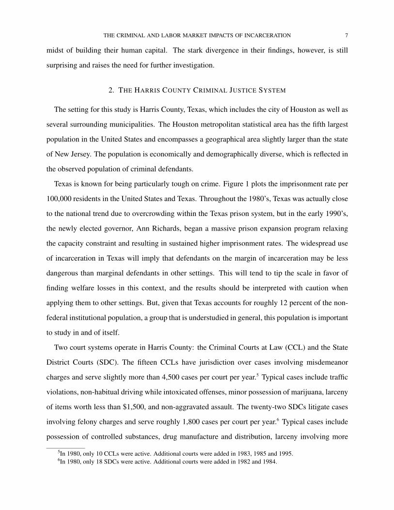
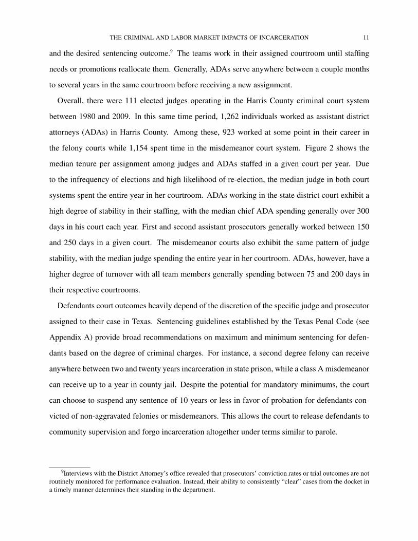
Texas is known for being particularly tough on crime. Figure 1 plots the imprisonment rate per
100,000 residents in the United States and Texas. Throughout the 1980’s, Texas was actually close
to the national trend due to overcrowding within the Texas prison system, but in the early 1990’s,
the newly elected governor, Ann Richards, began a massive prison expansion program relaxing
the capacity constraint and resulting in sustained higher imprisonment rates. The widespread use
of incarceration in Texas will imply that defendants on the margin of incarceration may be less
dangerous than marginal defendants in other settings. This will tend to tip the scale in favor of
finding welfare losses in this context, and the results should be interpreted with caution when
applying them to other settings. But, given that Texas accounts for roughly 12 percent of the non-
federal institutional population, a group that is understudied in general, this population is important
to study in and of itself.
Two court systems operate in Harris County: the Criminal Courts at Law (CCL) and the State
District Courts (SDC). The fifteen CCLs have jurisdiction over cases involving misdemeanor
charges and serve slightly more than 4,500 cases per court per year.5 Typical cases include traffic
violations, non-habitual driving while intoxicated offenses, minor possession of marijuana, larceny
of items worth less than $1,500, and non-aggravated assault. The twenty-two SDCs litigate cases
involving felony charges and serve roughly 1,800 cases per court per year.6 Typical cases include
possession of controlled substances, drug manufacture and distribution, larceny involving more
5In 1980, only 10 CCLs were active. Additional courts were added in 1983, 1985 and 1995.6In 1980, only 18 SDCs were active. Additional courts were added in 1982 and 1984.
8 MICHAEL MUELLER-SMITH
FIGURE 1. National versus Texas imprisonment rate per 100,000 residents
0
100
200
300
400
500
600
700
800
900
1978 1981 1984 1987 1990 1993 1996 1999 2002 2005 2008 2011
United States Texas
Source: Bureau of Justice Statistics, Corrections Statistical Analysis Tool.
than $1,500 in stolen property, residential or vehicular burglary, aggravated assault as well as more
heinous offenses like murder, rape and child abuse. The felony and misdemeanor courts are ad-
ministratively segregated yet physically co-located at the Harris County Criminal Justice Center
(1201 Franklin St., Houston, TX 77002).7
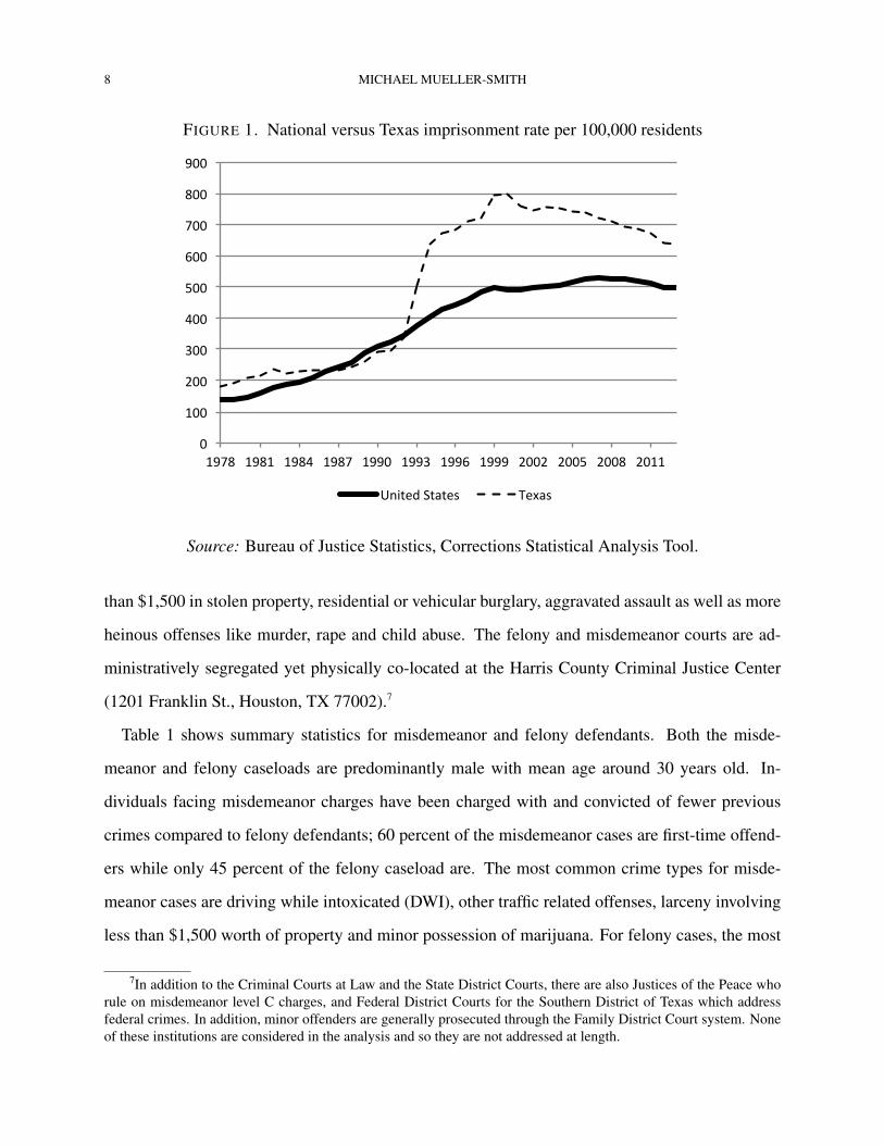
Table 1 shows summary statistics for misdemeanor and felony defendants. Both the misde-
meanor and felony caseloads are predominantly male with mean age around 30 years old. In-
dividuals facing misdemeanor charges have been charged with and convicted of fewer previous
crimes compared to felony defendants; 60 percent of the misdemeanor cases are first-time offend-
ers while only 45 percent of the felony caseload are. The most common crime types for misde-
meanor cases are driving while intoxicated (DWI), other traffic related offenses, larceny involving
less than $1,500 worth of property and minor possession of marijuana. For felony cases, the most
7In addition to the Criminal Courts at Law and the State District Courts, there are also Justices of the Peace whorule on misdemeanor level C charges, and Federal District Courts for the Southern District of Texas which addressfederal crimes. In addition, minor offenders are generally prosecuted through the Family District Court system. Noneof these institutions are considered in the analysis and so they are not addressed at length.
THE CRIMINAL AND LABOR MARKET IMPACTS OF INCARCERATION 9
common crimes are more serious drug possession (in terms of quantity or seriousness of the illicit
drugs), more costly property crimes, and aggravated assault.
Roughly equal shares of non-Hispanic Caucasian, non-Hispanic African American and Hispanic
defendants are represented in both caseloads. Misdemeanor cases have a relatively larger propor-
tion of non-Hispanic Caucasians, whereas felony cases are more likely to be African Americans. A
number of other physical descriptors are available in the data including: skin tone, height, weight,
body type, eye color and hair color. These are mainly recorded in the event a warrant needs to be
issued for the defendant. Coverage of these variables is much more reliable for cases from 1985
and onwards when record keeping in the court files improved.
When criminal charges are filed against a defendant in Harris County, his case is randomly
assigned to a courtroom.8 Randomization is viewed as an impartial assignment mechanism for de-
fendants and an equitable division of labor between courtrooms. Up to the late 1990s, assignment
was carried out using a bingo ball roller; this was later transitioned to a computerized system for
automatic random case assignment. In order to ensure the case allocation mechanism is not ma-
nipulated by internal actors, the Harris County District Clerk’s office, which is both physically and
administratively segregated from the criminal court system, is solely responsible for courtroom
assignment.
When a case is randomly assigned to a courtroom, a defendant is assigned to the jurisdiction of
a specific judge and team of assistant district attorneys. The judges are elected to serve a specific
bench and are responsible for presiding over all cases assigned to their courtroom while in office.
Elections occur every two years, and the vast majority of judges are successfully reelected. As a
result, a defendant’s initial court assignment will likely determine the judge who presides over the
entirety of his trial.
The Harris County District Attorney’s office stations a team of three assistant district attorneys
(one chief ADA and two subordinate ADAs) to each CCL and SDC. This team prosecutes all cases
assigned to their courtroom with broad discretion over how to divide the workload within the team
8Two types of cases do not undergo random assignment. If a defendant is already on probation from a specificcourt, his new charges will automatically be assigned to that same courtroom. In addition, charges at the CapitalFelony level are not randomly assigned because they generally require significant resources to adjudicate. Becauseneither of these types of charges are randomly assigned, they are dropped from the analysis.
10 MICHAEL MUELLER-SMITH
TABLE 1. Characteristics of Harris County’s Criminal Courts at Law andState District Courts’ caseloads, 1980-2009
Criminal Court at Law State District CourtDefendant Characteristics (Misdemeanor Offenses) (Felony Offenses)
Male 0.78 0.81Age 29.84 30.26First time offender 0.61 0.45Total prior felony charges 0.44 0.93Total prior misdemeanor charges 0.8 1.2Type of criminal charge
Driving while intoxicated 0.25 0.04Traffic 0.11 0.01Drug possession 0.11 0.26Drug manufacture or distribution 0 0.09Property 0.23 0.31Violent 0.09 0.13
Median duration of trial (months) 1.35 2.14Race/Ethnicity
Caucasian 0.39 0.30African American 0.31 0.46Hispanic 0.29 0.23Other 0.01 0.01
Skin toneFair 0.14 0.13Light 0.06 0.05Light brown 0.07 0.06Medium 0.22 0.22Medium brown 0.09 0.1Olive 0.03 0.03Dark 0.04 0.07Dark brown 0.09 0.14Black 0.04 0.07Missing 0.21 0.13
Height (in.) 68.13 68.4Weight (lbs.) 169.82 172.51Body type
Skinny, light 0.11 0.13Medium 0.6 0.66Heavy, obese 0.08 0.09Missing 0.21 0.13
Eye colorGreen, blue 0.18 0.15Brown, black 0.65 0.75Missing 0.17 0.1
Hair colorBlonde, red 0.07 0.06Black, brown 0.75 0.83Bald, grey 0.02 0.02Missing 0.17 0.1
Total cases 1,449,453 775,576
Source: Author’s calculations using Harris County District Clerk’s criminal courtrecords.Notes: Calculations do not include sealed court records, juvenile offenders or defen-dants charged with capital murder.
THE CRIMINAL AND LABOR MARKET IMPACTS OF INCARCERATION 11
and the desired sentencing outcome.9 The teams work in their assigned courtroom until staffing
needs or promotions reallocate them. Generally, ADAs serve anywhere between a couple months
to several years in the same courtroom before receiving a new assignment.
Overall, there were 111 elected judges operating in the Harris County criminal court system
between 1980 and 2009. In this same time period, 1,262 individuals worked as assistant district
attorneys (ADAs) in Harris County. Among these, 923 worked at some point in their career in
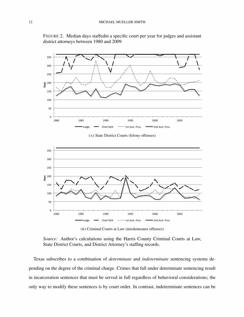
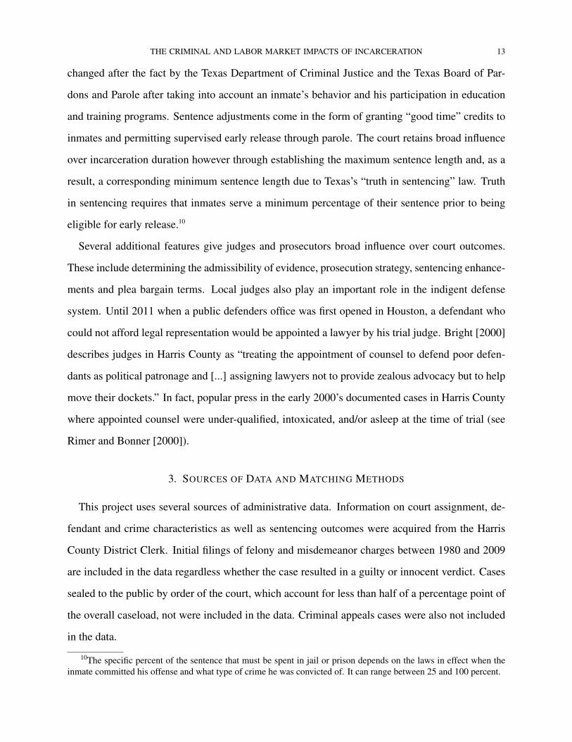
the felony courts while 1,154 spent time in the misdemeanor court system. Figure 2 shows the
median tenure per assignment among judges and ADAs staffed in a given court per year. Due
to the infrequency of elections and high likelihood of re-election, the median judge in both court
systems spent the entire year in her courtroom. ADAs working in the state district court exhibit a
high degree of stability in their staffing, with the median chief ADA spending generally over 300
days in his court each year. First and second assistant prosecutors generally worked between 150
and 250 days in a given court. The misdemeanor courts also exhibit the same pattern of judge
stability, with the median judge spending the entire year in her courtroom. ADAs, however, have a
higher degree of turnover with all team members generally spending between 75 and 200 days in
their respective courtrooms.
Defendants court outcomes heavily depend of the discretion of the specific judge and prosecutor
assigned to their case in Texas. Sentencing guidelines established by the Texas Penal Code (see
Appendix A) provide broad recommendations on maximum and minimum sentencing for defen-
dants based on the degree of criminal charges. For instance, a second degree felony can receive
anywhere between two and twenty years incarceration in state prison, while a class A misdemeanor
can receive up to a year in county jail. Despite the potential for mandatory minimums, the court
can choose to suspend any sentence of 10 years or less in favor of probation for defendants con-
victed of non-aggravated felonies or misdemeanors. This allows the court to release defendants to
community supervision and forgo incarceration altogether under terms similar to parole.
9Interviews with the District Attorney’s office revealed that prosecutors’ conviction rates or trial outcomes are notroutinely monitored for performance evaluation. Instead, their ability to consistently “clear” cases from the docket ina timely manner determines their standing in the department.
12 MICHAEL MUELLER-SMITH
FIGURE 2. Median days staffedin a specific court per year for judges and assistantdistrict attorneys between 1980 and 2009
0
50
100
150
200
250
300
350
1980 1985 1990 1995 2000 2005
Days
Judge Chief ADA 1st Asst. Pros. 2nd Asst. Pros.
(A) State District Courts (felony offenses)
0
50
100
150
200
250
300
350
1980 1985 1990 1995 2000 2005
Days
Judge Chief ADA 1st Asst. Pros. 2nd Asst. Pros.
(B) Criminal Courts at Law (misdemeanor offenses)
Source: Author’s calculations using the Harris County Criminal Courts at Law,State District Courts, and District Attorney’s staffing records.
Texas subscribes to a combination of determinate and indeterminate sentencing systems de-
pending on the degree of the criminal charge. Crimes that fall under determinate sentencing result
in incarceration sentences that must be served in full regardless of behavioral considerations; the
only way to modify these sentences is by court order. In contrast, indeterminate sentences can be
THE CRIMINAL AND LABOR MARKET IMPACTS OF INCARCERATION 13
changed after the fact by the Texas Department of Criminal Justice and the Texas Board of Par-
dons and Parole after taking into account an inmate’s behavior and his participation in education
and training programs. Sentence adjustments come in the form of granting “good time” credits to
inmates and permitting supervised early release through parole. The court retains broad influence
over incarceration duration however through establishing the maximum sentence length and, as a
result, a corresponding minimum sentence length due to Texas’s “truth in sentencing” law. Truth
in sentencing requires that inmates serve a minimum percentage of their sentence prior to being
eligible for early release.10
Several additional features give judges and prosecutors broad influence over court outcomes.
These include determining the admissibility of evidence, prosecution strategy, sentencing enhance-
ments and plea bargain terms. Local judges also play an important role in the indigent defense
system. Until 2011 when a public defenders office was first opened in Houston, a defendant who
could not afford legal representation would be appointed a lawyer by his trial judge. Bright [2000]
describes judges in Harris County as “treating the appointment of counsel to defend poor defen-
dants as political patronage and [...] assigning lawyers not to provide zealous advocacy but to help
move their dockets.” In fact, popular press in the early 2000’s documented cases in Harris County
where appointed counsel were under-qualified, intoxicated, and/or asleep at the time of trial (see
Rimer and Bonner [2000]).
3. SOURCES OF DATA AND MATCHING METHODS
This project uses several sources of administrative data. Information on court assignment, de-
fendant and crime characteristics as well as sentencing outcomes were acquired from the Harris
County District Clerk. Initial filings of felony and misdemeanor charges between 1980 and 2009
are included in the data regardless whether the case resulted in a guilty or innocent verdict. Cases
sealed to the public by order of the court, which account for less than half of a percentage point of
the overall caseload, not were included in the data. Criminal appeals cases were also not included
in the data.
10The specific percent of the sentence that must be spent in jail or prison depends on the laws in effect when theinmate committed his offense and what type of crime he was convicted of. It can range between 25 and 100 percent.
14 MICHAEL MUELLER-SMITH
For the purpose of the analysis, defendants charged with multiple criminal offenses or recharged
for the same crime after a mistrial were collapsed to a single observation. For these cases, only the
earliest filing date and original sentencing outcomes outcomes were retained. For all defendants,
sentencing modifications were eliminated from the data (e.g. a defendant who violated the terms
of his probation after three years and was incarcerated as a result was only coded as only receiving
probation in his original sentencing).
Administrative identifiers in the court data link defendants to their full historical criminal record
in Harris County, allowing the research to evaluate local recidivism outcomes. Archival research
gathered judge tenure and assistant district attorney staffing documents from the courts and tran-
scribed the information into an electronic database. Judges and assistant district attorneys were
then mapped to criminal court cases using the defendant’s filing date and assigned court number.
Data on actual incarceration spans between 1978 and 2013 were acquired through Public Infor-
mation Act requests from the Texas Department of Criminal Justice for state prisons and from the
Harris County Sheriff’s Office for the Harris County Jail, and matched using the defendant’s full
name and date of birth.
Quarterly unemployment insurance wage records for the entire state of Texas between 1994
and 2012 were accessed through a data sharing agreement with the Texas Workforce Commission.
Monthly Food Stamps and Temporary Assistance for Needy Families benefits between 1994/1992
and 2011 were accessed through a data sharing agreement with the Texas Health and Human
Services Commission. Matching between the various data sources was based on a combination of
full name, sex, exact date of birth and social security number depending on what variables were
available in each specific dataset.
Public marriage and divorce indices were also collected from the Texas Department of State
Health Services. Unfortunately, this data is only identified at the full name and age at marriage or
divorce level, making it prone to mismatch. Incorrect data linkages should be orthogonal to court-
room assignment which should lead to classic measurement error and push estimated coefficients
towards zero.
THE CRIMINAL AND LABOR MARKET IMPACTS OF INCARCERATION 15
4. THE COMPLICATIONS OF MULTIDIMENSIONAL AND NON-MONOTONIC SENTENCING
To evaluate the impact of incarceration, this study relies on exogenous variation in sentencing
outcomes attributable to random assignment of defendants to criminal courts. Prior work using
this research design has generally been formalized using the following two equations:
Yi = β0 + β1(Xi)Di + β2Xi + εi ,(1)
Di = γ0 + γ1Ji + γ2Xi + νi ,(2)
where,
E[εi, νi|Xi] 6= 0 , E[εi, Ji|Xi] = 0 and γ1 6= 0 .
In this notation, Yi is the outcome variable, Di is a criminal sentence (such as an indicator vari-
able for being incarcerated or a continuous measure of the duration of incarceration), Xi is the
observed defendant characteristics and Ji is a vector of dummy variables for the defendant’s ran-
domly assigned judge.11 The program effect can potentially be heterogeneous so β1(Xi) is allowed
to depend on defendant traits. Non-zero coefficients in γ1 indicate differences in average sentenc-
ing outcomes between judges who serve statistically equivalent populations. Such differences are
often motivated on the basis that some judges are thought to be “tough” while others are “easy” on
defendants.
Two additional assumptions are required in order to achieved unbiased results (see Imbens and
Angrist [1994], Angrist et al. [1996]). First, the exclusion restriction requires thatE[Yi|Di, Xi, Ji] =
E[Yi|Di, Xi, J′i ]. This means that judge assignment can only impact the final outcome through its
influence on the criminal sentence. The second requirement is that the data must satisfy a mono-
tonicity assumption: {E[Di|Xi, Ji = j] ≥ E[Di|Xi, Ji = k] ∀i or E[Di|Xi, Ji = j] ≤ E[Di|Xi, Ji = k] ∀i} ∀j, k.
This means that defendants assigned to judges with higher overall incarceration rates must also be
at weakly higher risk for incarceration if assigned to their caseload.
11In the specific context of this study, random court assignment results in both a random judge as well as a randomteam of assistant district attorneys. For the ease of notation and to remain consistent with the existing literature,however, I proceed using only judges in the model but knowing that they are a placeholder for all influential actorsthat are attached to a specific courtroom.
16 MICHAEL MUELLER-SMITH
The parsimony of this standard model makes it quite appealing. The source of identification
is intuitive, and the estimation is generally straightforward, particularly in settings where the re-
searcher is constrained by data availability. The fact that my data exhibits multidimensional and
non-monotonic sentencing patterns, however, limits the plausibility of satisfying the necessary as-
sumptions for unbiasedness. Instead, application of the standard methods in this context results in
two distinct biases which for the sake of clarity I term omitted treatment bias and non-monotonic
instruments bias. The nature of these biases are described below.
Omitted treatment bias. In the Texas criminal justice system, judges and prosecutors have influ-
ence over several aspects of trial outcomes (e.g. guilt or innocence, incarceration versus probation,
duration of punishment, amount of fine, etc.). I may, however, only be interested in a subset of
the full range of sentencing outcomes just as incarceration is the focus of this present study. To
distinguish between these sets, I define Dfi ⊂ Di as the focal set of sentencing outcomes, while
the remaining elements are the non-focal set Dni .
Omitted treatment bias is the result of neglecting of Dni when estimating the causal effect of
Dfi on Yi. Judicial tendencies on focal and non-focal sentencing outcomes may be correlated
leading to violations of the exclusion restriction. For instance, if judges who have higher than
average incarceration rates also are more likely to impose fines (and the estimated model omits
fines), the estimated impact of incarceration will capture a weighted sum of the combined effect
of incarceration and fines. It is unrealistic to think that researchers ever observe the full set of
potential treatments a defendant may received. For instance, a judge may speak sternly to the
defendant, which would likely not be measured in the data. But, to the extent that unmeasured
treatments play minor roles in producing final outcomes and are uncorrelated with other judicial
tendencies, the potential bias is minimal.12
12Compared to other settings, like research on the impact of going to a better school where treatments may in-clude complex interactions between various school inputs and peer interactions, the criminal justice context relativelystraightforward with respect to what the major components of Di should include. These are: incarceration status andlength, fine status and amount, probation status and length, and less common enrollment in alternative sentencingprograms like electronic monitoring, drug treatment, boot camps, or driver’s education. Since there is little to nointeraction among defendants in the court room setting, there is minimal concern for peer influence at this stage.
THE CRIMINAL AND LABOR MARKET IMPACTS OF INCARCERATION 17
Omitted treatment bias can be easily avoided by estimating to the full model, inclusive of both
Dfi and Dn
i . In this scenario, both the focal and non-focal elements of Di would be simultane-
ously instrumented using random assignment of judges as the source of exogenous variation. This
would ensure that, for instance, the impact of incarceration is identified off of judges who tend to
incarcerate relatively more after accounting for their other sentencing tendencies. This approach,
however, may undermine joint tests of the first stage and weak instrument robust inference for the
focal variables since some non-focal sentencing outcomes may not exhibit significant differences
between judges.
To solve this problem, this study proposes constructing predicted values of E[Dni |Ji, Xi] and
adding them to the second stage equation to eliminate the omitted treatment bias. In practice, this
entails estimating the first stage equation for each element of Dni , and then adding the predicted
values to the second stage equation as reduced form controls.
Non-monotonic instruments bias. Non-monotonic sentencing patterns also create opportunities
for bias. Some judges, for instance, are observed to have higher than average incarceration rates
for specific subsets of their caseload like drug offenders while also exhibiting lower than average
incarceration rates for other groups like property offenders. This creates a situation where it is
no longer necessarily true that being randomly assigned to a judge with a higher overall rate of
incarceration actually increases the probability of incarceration for every defendant. Violations
of the monotonicity assumption lead to an unsigned bias making it difficult to determine if the
estimates under- or over-estimate the true effect.
To the extant that this complexity responds to observable characteristics, it is not insurmount-
able. The standard approach might result in biased estimates, but that is a consequence of the fact
that the standard model is misspecified in this context. Judges form expectations as to what will
best maximize their objective function given the facts of the case before them and their own sub-
jective information. They don’t simply see defendants interchangeably, but respond to the specific
context of each case. This is not saying that judges are inconsistent in their application of the law;
instead, their decision rules are just more complex that mean shifts between judges.
18 MICHAEL MUELLER-SMITH
The alternative first stage equation I propose for this sentencing model is:
Di = Γ0 + Γ1(Xi)Ji + Γ2Xi + νi .(3)
In contrast to Equation 2, Equation 3 allows judicial preference to flexibly adjust according to
defendant characteristics. The implication is that the monotonicity of the impact of judge assign-
ment no longer need hold across all defendants, but instead the impact of judge assignment must
only remain consistent among a group of peers with similar observable characteristics (e.g. Cau-
casian male drug offenders or African American females convicted of driving while intoxicated).13
While the modified approach adds complexity to the model, it relaxes the assumptions necessary
for unbiased results.
Empirical examples. To illustrate how the multidimensional and non-monotonic sentencing af-
fect my estimates, I construct two examples using actual court data from Harris County, TX. The
first example considers the impact of accounting for additional degrees of treatment the second
demonstrates how non-uniformities in sentencing can generate bias. The estimates shown in these
examples are given to illustrate the features of the data; more refined estimates using the full sample
of data are reserved for Section 7.
The first example estimates the “causal” impact of incarceration on one year recidivism rates
in the felony caseload. The analysis uses all individuals who were charged with felony crimes
between 2005 and 2006, and their court sentence is instrumented using their randomly assigned
judge. While the coefficient of primary interest is a dummy variable measuring whether or not
a defendant was incarcerated for any period of time, each specification progressively adds more
controls for non-focal dimensions of sentencing to the model. The controls in this example are
constructed using the judge-specific mean of each non-focal court outcome. The results are shown
in Table 2.
13A more general model could adopt a random effects framework to account for unobserved variation as well (seeHeckman and Vytlacil [1998] and Wooldridge [1997, 2003]), but is beyond the scope of this study.
THE CRIMINAL AND LABOR MARKET IMPACTS OF INCARCERATION 19
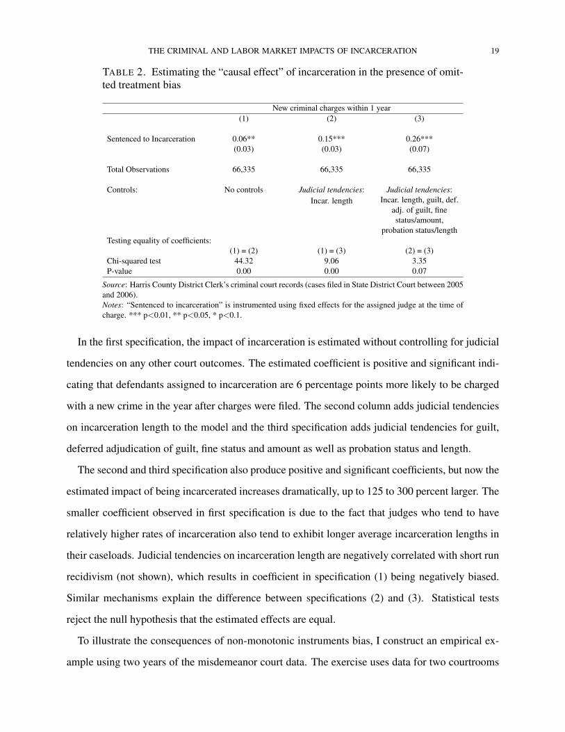
TABLE 2. Estimating the “causal effect” of incarceration in the presence of omit-ted treatment bias
New criminal charges within 1 year(1) (2) (3)
Sentenced to Incarceration 0.06** 0.15*** 0.26***(0.03) (0.03) (0.07)
Total Observations 66,335 66,335 66,335
Controls: No controls Judicial tendencies:Incar. length
Judicial tendencies:Incar. length, guilt, def.
adj. of guilt, finestatus/amount,
probation status/lengthTesting equality of coefficients:
(1) = (2) (1) = (3) (2) = (3)Chi-squared test 44.32 9.06 3.35P-value 0.00 0.00 0.07
Source: Harris County District Clerk’s criminal court records (cases filed in State District Court between 2005and 2006).Notes: “Sentenced to incarceration” is instrumented using fixed effects for the assigned judge at the time ofcharge. *** p<0.01, ** p<0.05, * p<0.1.
In the first specification, the impact of incarceration is estimated without controlling for judicial
tendencies on any other court outcomes. The estimated coefficient is positive and significant indi-
cating that defendants assigned to incarceration are 6 percentage points more likely to be charged
with a new crime in the year after charges were filed. The second column adds judicial tendencies
on incarceration length to the model and the third specification adds judicial tendencies for guilt,
deferred adjudication of guilt, fine status and amount as well as probation status and length.
The second and third specification also produce positive and significant coefficients, but now the
estimated impact of being incarcerated increases dramatically, up to 125 to 300 percent larger. The
smaller coefficient observed in first specification is due to the fact that judges who tend to have
relatively higher rates of incarceration also tend to exhibit longer average incarceration lengths in
their caseloads. Judicial tendencies on incarceration length are negatively correlated with short run
recidivism (not shown), which results in coefficient in specification (1) being negatively biased.
Similar mechanisms explain the difference between specifications (2) and (3). Statistical tests
reject the null hypothesis that the estimated effects are equal.
To illustrate the consequences of non-monotonic instruments bias, I construct an empirical ex-
ample using two years of the misdemeanor court data. The exercise uses data for two courtrooms
20 MICHAEL MUELLER-SMITH
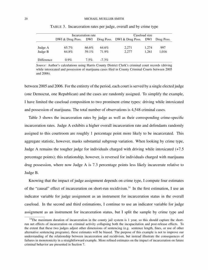
TABLE 3. Incarceration rates per judge, overall and by crime type
Incarceration rate Caseload sizeDWI & Drug Poss. DWI Drug Poss. DWI & Drug Poss. DWI Drug Poss.
Judge A 65.7% 66.6% 64.6% 2,271 1,274 997Judge B 64.8% 59.1% 71.9% 2,277 1,261 1,016
Difference 0.9% 7.5% -7.3%
Source: Author’s calculations using Harris County District Clerk’s criminal court records (drivingwhile intoxicated and possession of marijuana cases filed in County Criminal Courts between 2005and 2006).
between 2005 and 2006. For the entirety of the period, each court is served by a single elected judge
(one Democrat, one Republican) and the cases are randomly assigned. To simplify the example,
I have limited the caseload composition to two prominent crime types: driving while intoxicated
and possession of marijuana. The total number of observations is 4,548 criminal cases.
Table 3 shows the incarceration rates by judge as well as their corresponding crime-specific
incarceration rates. Judge A exhibits a higher overall incarceration rate and defendants randomly
assigned to this courtroom are roughly 1 percentage point more likely to be incarcerated. This
aggregate statistic, however, masks substantial subgroup variation. When looking by crime type,
Judge A remains the tougher judge for individuals charged with driving while intoxicated (+7.5
percentage points); this relationship, however, is reversed for individuals charged with marijuana
drug possession, where now Judge A is 7.3 percentage points less likely incarcerate relative to
Judge B.
Knowing that the impact of judge assignment depends on crime type, I compute four estimates
of the “causal” effect of incarceration on short-run recidivism.14 In the first estimation, I use an
indicator variable for judge assignment as an instrument for incarceration status in the overall
caseload. In the second and third estimations, I continue to use an indicator variable for judge
assignment as an instrument for incarceration status, but I split the sample by crime type and
14The maximum duration of incarceration in the county jail system is 1 year, so this should capture the short-run net effects of incarceration on criminal activity collapsing both the incapacitation and post-release effects. Tothe extent that these two judges adjust other dimensions of sentencing (e.g. sentence length, fines, or use of otheralternative sentencing programs), these estimates will be biased. The purpose of this example is not to improve ourunderstanding of the relationship between incarceration and recidivism, but instead illustrate the consequences offailures in monotonicity in a straightforward example. More refined estimates on the impact of incarceration on futurecriminal behavior are presented in Section 7.
THE CRIMINAL AND LABOR MARKET IMPACTS OF INCARCERATION 21
estimate the impact separately. In the final estimation, I use interactions between judge assignment
and crime type as instruments for incarceration.
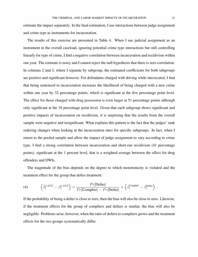
The results of this exercise are presented in Table 4. When I use judicial assignment as an
instrument in the overall caseload, ignoring potential crime type interactions but still controlling
linearly for type of crime, I find a negative correlation between incarceration and recidivism within
one year. The estimate is noisy and I cannot reject the null hypothesis that there is zero correlation.
In columns 2 and 3, where I separate by subgroup, the estimated coefficients for both subgroups
are positive and significant however. For defendants charged with driving while intoxicated, I find
that being sentenced to incarceration increases the likelihood of being charged with a new crime
within one year by 32 percentage points, which is significant at the five percentage point level.
The effect for those charged with drug possession is even larger at 51 percentage points although
only significant at the 10 percentage point level. Given that each subgroup shows significant and
positive impacts of incarceration on recidivism, it is surprising that the results from the overall
sample were negative and insignificant. What explains this pattern is the fact that the judges’ rank
ordering changes when looking at the incarceration rates for specific subgroups. In fact, when I
return to the pooled sample and allow the impact of judge assignment to vary according to crime
type, I find a strong correlation between incarceration and short-run recidivism (41 percentage
points), significant at the 1 percent level, that is a weighted average between the effect for drug
offenders and DWIs.
The magnitude of the bias depends on the degree to which monotonicity is violated and the
treatment effect for the group that defies treatment:
(4)(βLATE1 − βLATE1
)=
Pr[Defier]Pr[Complier]− Pr[Defier]
×(βComplier1 − βDefier
1
).
If the probability of being a defier is close to zero, then the bias will also be close to zero. Likewise,
if the treatment effects for the group of compliers and defiers is similar, the bias will also be
negligible. Problems arise, however, when the ratio of defiers to compliers grows and the treatment
effects for the two groups systematically differ.
22 MICHAEL MUELLER-SMITH
TABLE 4. Estimating the “causal effect” of incarceration in the presence of non-monotonic instruments bias
New criminal charges within 1 year
Sentenced to Incarceration -0.31 0.32** 0.51* 0.41***(1.31) (0.16) (0.28) (0.15)
Crime type = DWI -0.21*** -0.17***(0.072) (0.014)
N 4,548 2,535 2,013 4,548
Sample DWI and Drug DWI Drug DWI and DrugInstrument Judge Judge Judge Judge × Crime
Anderson canon. Correlation LM statistic 0.46 15.2 12.2 27.4Cragg-Donald Wald F statistic 0.46 15.3 12.3 13.8
Source: Author’s calculations using Harris County District Clerk’s criminal court records (driv-ing while intoxicated and possession of marijuana cases filed in County Criminal Courts between2005 and 2006).Notes: *** p<0.01, ** p<0.05, * p<0.1.
Given this formula, I can directly compute the magnitude of the bias from using the judge assign-
ment without crime type interactions as an instrument. This requires estimating four parameters:
Pr[Complier], Pr[Defier], βComplier1 and βDefier
1 . The compliers in this example are a subset of the
individuals charged with driving while intoxicated while the defiers are those charged with posses-
sion of marijuana. The complier rate will be equal to difference in the incarceration rates between
the judges for DWI’s (0.0748) times the percent of the sample that is charged with DWI (0.557).
The defier rate is equal to difference in the incarceration rates between the judges for drug posses-
sion (0.0726) times the percent of the sample that is charged with DWI (0.443). For the remaining
two parameters, βComplier1 is shown in the second column of Table 4, while βDefier
1 is listed in the
third column. This results in the following calculation:
Bias =0.0726× 0.443
0.0748× 0.557− 0.0726× 0.443× (0.3248− 0.5147)
= −0.6367
THE CRIMINAL AND LABOR MARKET IMPACTS OF INCARCERATION 23
When adding together the impact of incarceration for individuals charged with driving while intox-
icated (e.g. the compliers in the example) with the estimate of the bias, I recover the point estimate
recorded in column 1 of Table 4 (i.e. βDWI + Bias = −0.31).
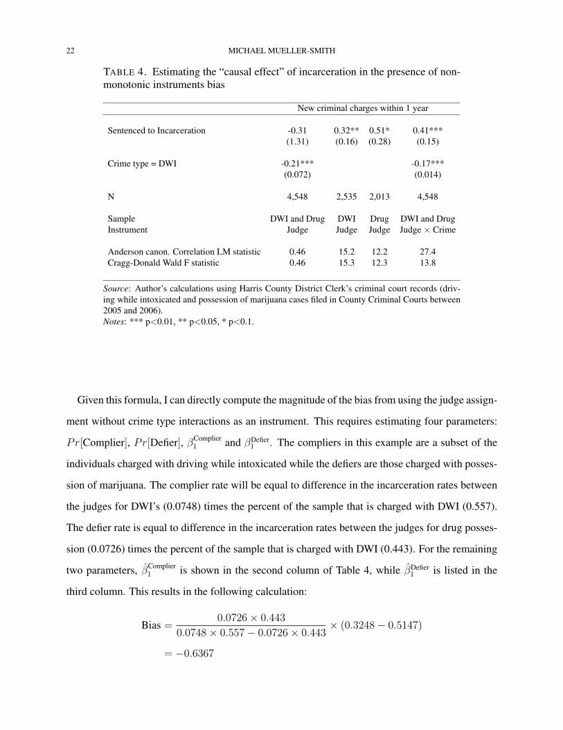
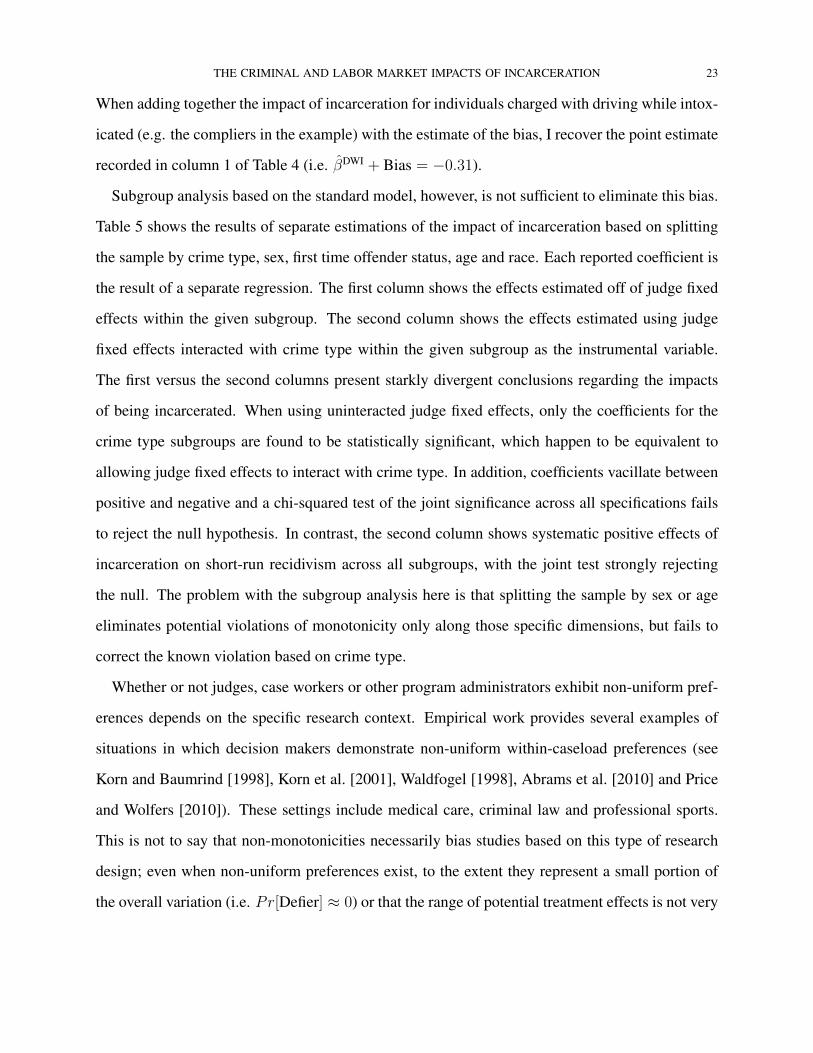
Subgroup analysis based on the standard model, however, is not sufficient to eliminate this bias.
Table 5 shows the results of separate estimations of the impact of incarceration based on splitting
the sample by crime type, sex, first time offender status, age and race. Each reported coefficient is
the result of a separate regression. The first column shows the effects estimated off of judge fixed
effects within the given subgroup. The second column shows the effects estimated using judge
fixed effects interacted with crime type within the given subgroup as the instrumental variable.
The first versus the second columns present starkly divergent conclusions regarding the impacts
of being incarcerated. When using uninteracted judge fixed effects, only the coefficients for the
crime type subgroups are found to be statistically significant, which happen to be equivalent to
allowing judge fixed effects to interact with crime type. In addition, coefficients vacillate between
positive and negative and a chi-squared test of the joint significance across all specifications fails
to reject the null hypothesis. In contrast, the second column shows systematic positive effects of
incarceration on short-run recidivism across all subgroups, with the joint test strongly rejecting
the null. The problem with the subgroup analysis here is that splitting the sample by sex or age
eliminates potential violations of monotonicity only along those specific dimensions, but fails to
correct the known violation based on crime type.
Whether or not judges, case workers or other program administrators exhibit non-uniform pref-
erences depends on the specific research context. Empirical work provides several examples of
situations in which decision makers demonstrate non-uniform within-caseload preferences (see
Korn and Baumrind [1998], Korn et al. [2001], Waldfogel [1998], Abrams et al. [2010] and Price
and Wolfers [2010]). These settings include medical care, criminal law and professional sports.
This is not to say that non-monotonicities necessarily bias studies based on this type of research
design; even when non-uniform preferences exist, to the extent they represent a small portion of
the overall variation (i.e. Pr[Defier] ≈ 0) or that the range of potential treatment effects is not very
24 MICHAEL MUELLER-SMITH
TABLE 5. Estimated impact of incarceration using Judge versusJudge × Crime fixed effects as instrumental variables
Sugroup N New criminal charges within 1 year
DWI 2,535 0.32** 0.32**(0.16) (0.16)
Drug Poss. 2,013 0.51* 0.51*(0.28) (0.28)
Female 682 0.88 0.31*(0.66) (0.17)
Male 3,866 0.27 0.48**(0.56) (0.20)
First 2,434 0.087 0.19(0.73) (0.14)
Repeat 2,114 -0.065 0.77*(1.23) (0.46)
Age < 25 1,919 0.75 0.45*(0.67) (0.24)
Age >= 25 2,625 0.33 0.37*(0.32) (0.20)
White 1,656 -0.36 0.23(1.34) (0.19)
Black 1,195 2.30 1.01*(3.95) (0.61)
Hispanic 1,697 0.90 0.26(1.38) (0.18)
Chi-squared test of joint significance 10.87 89.11P-value 0.45 0.00
Incarceration rateby Judge
Incarceration rateby Judge ×Crime type
Instrumental Variable:
Source: Author’s calculations using Harris County District Clerk’s criminalcourt records (driving while intoxicated and possession of marijuana cases filedin County Criminal Courts between 2005 and 2006).Notes: *** p<0.01, ** p<0.05, * p<0.1.
large, the resulting bias will be minimal. It does, however, provide motivation for developing more
rigorous empirical methods.
5. ESTIMATING INSTRUMENTAL VARIABLE MODELS IN THE PRESENCE OF
NON-MONOTONIC INSTRUMENTS
The solution to non-uniform judge preferences is straightforward if judges base their decisions
on a single defendant characteristic that is categorical in nature (e.g. crime type). Using the
judges’ crime-specific incarceration rates in lieu of their average incarceration rates as the source
THE CRIMINAL AND LABOR MARKET IMPACTS OF INCARCERATION 25
of exogenous variation in sentencing will eliminate monotonicity violations resulting from the
non-uniform preferences. But, the answer becomes more complicated when the data contains
many defendant characteristics some of which might be categorical (e.g. sex, race or skin tone)
and others might be continuous (e.g. age, time since last criminal charge or total prior convictions)
and it is unknown over which judges base their decisions.
A fully non-parametric estimation of Γ1(Xi) from Equation 3 would be the most straightforward
approach from a theoretical perspective. Multivariate regression including screener fixed effects
fully interacted with all potential pre-existing covariates and combinations thereof would provide
consistent estimates of the flexible judge-specific decision rules. But, due to the curse of dimen-
sionality such models often are not practical. The problem could be simplified if the combination
of traits included as interactions with judge assignment were pre-specified, which could be mo-
tivated by detailed institutional knowledge of research setting. However, putting this choice in
the hands of the researcher unfortunately opens the door to undisciplined specification searching
which limits the reliability of the produced estimates.
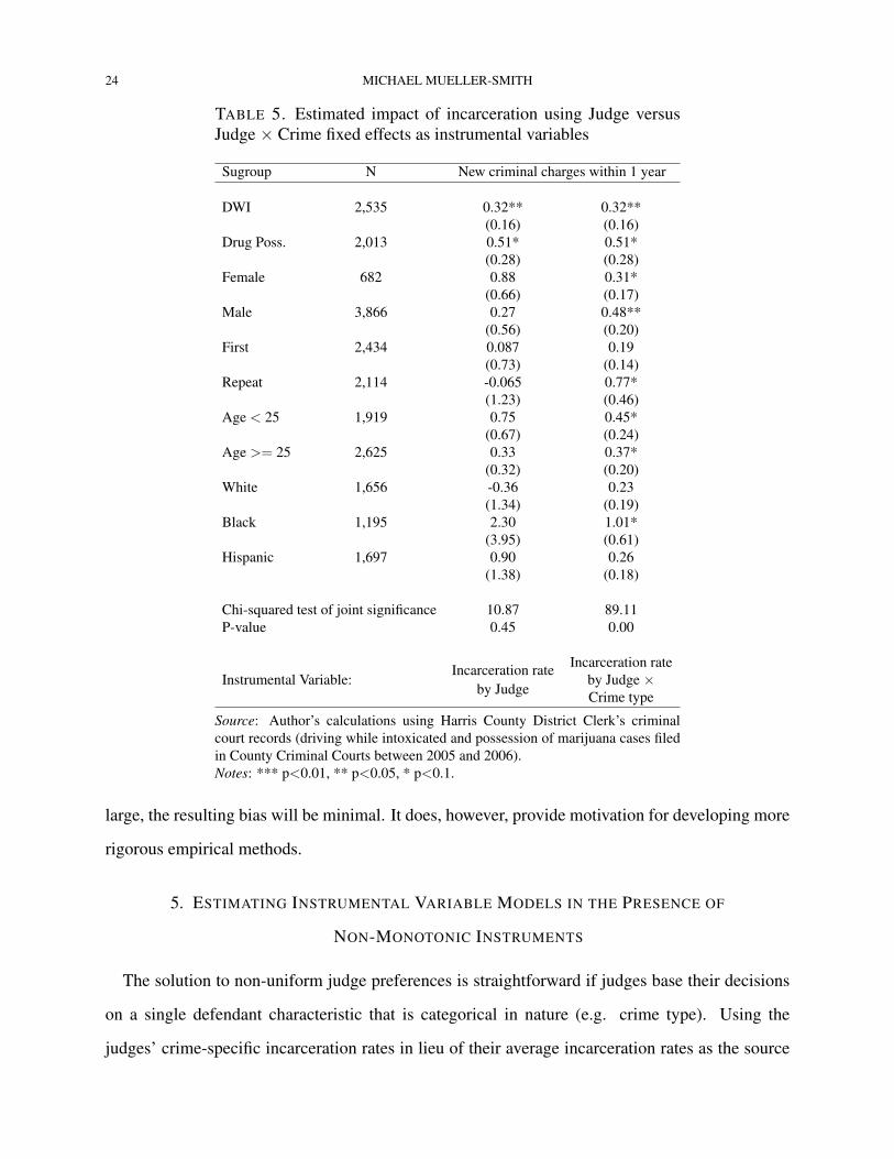
A semi-parametric approach where Γ1(Xi) is approximated in a linear model using a series of
basis functions provides a feasible compromise. In this framework,
Γ1(Xi)Ji =K∑k=1
ωkbk(Xi, Ji) + ηi,(5)
where bk(·) is a basis function using information on defendant traits (Xi) and judge assignment
(Ji) that measures relative judicial preferences, the parameters ωk provide weights to each bk(·)
and ηi is an approximation error.
Any number of basis functions could be utilized here. The functions I focus on measure how
judicial preferences deviate from caseload wide trends after conditioning on various combinations
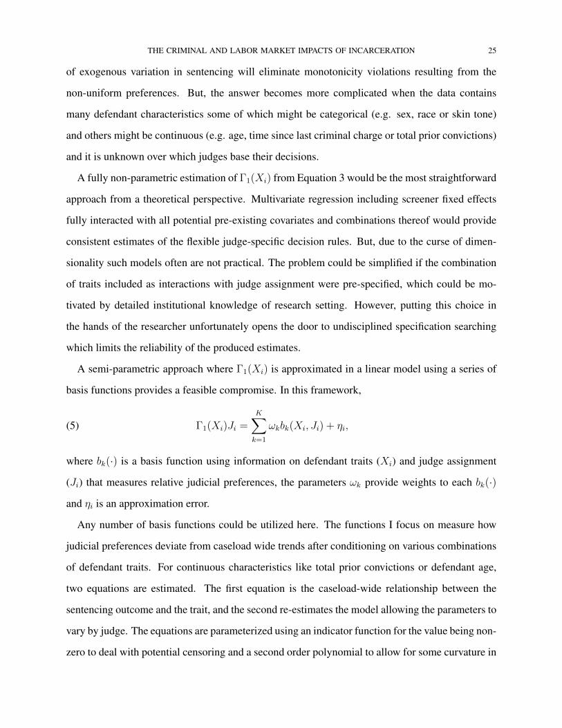
of defendant traits. For continuous characteristics like total prior convictions or defendant age,
two equations are estimated. The first equation is the caseload-wide relationship between the
sentencing outcome and the trait, and the second re-estimates the model allowing the parameters to
vary by judge. The equations are parameterized using an indicator function for the value being non-
zero to deal with potential censoring and a second order polynomial to allow for some curvature in
26 MICHAEL MUELLER-SMITH
preferences:
Di = φ01[xi > 0] + φ1xi + φ2x2i + ei ,
Di =∑j∈J
[φj01[xi > 0] + φj1xi + φj2x
2i
]× 1[Ji = j] + ei .
The candidate basis function bk(·) is then computed by taking the difference between the predicted
value of Di based on the judge-specific and general model. To avoid any degree of mechani-
cal correlation in the first stage, several researchers have recommended using “leave-one-out” or
“jackknife” estimators wherein data for all defendants except for individual i are used to estimate
bk(·) for individual i (see Kling [2006], Doyle [2007], and Aizer and Doyle [2013]). One can im-
plement this strategy without having to reestimate the two models for each observation by simply
computing the diagonal elements of the Hessian matrix Hk. The value hk;ii, which represents the
ith diagonal element of Hk, measures the impact that observation i has on his predicted value,
which is known in statistics as i’s leverage. The jackknife residual is then be reverse engineered
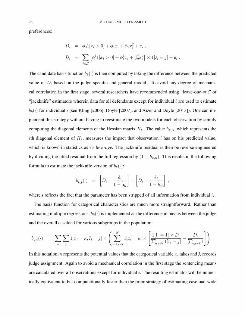
by dividing the fitted residual from the full regression by (1 − hk,ii). This results in the following
formula to estimate the jackknife version of bk(·):
bk,i(·) =
[Di −
ei1− hii
]−[Di −
ei
1− hii
],
where i reflects the fact that the parameter has been stripped of all information from individual i.
The basis function for categorical characteristics are much more straightforward. Rather than
estimating multiple regressions, bk(·) is implemented as the difference in means between the judge
and the overall caseload for various subgroups in the population:
bk,i(·) =∑κ
∑j
1[xi = κ, Ji = j]×
(N∑
ι=1,ι 6=i
1[xι = κ]×
[1[Jι = 1]×Dι∑ι,ι6=i 1[Jι = j]
− Dι∑ι,ι6=i 1
]).
In this notation, κ represents the potential values that the categorical variable xi takes and Ji records
judge assignment. Again to avoid a mechanical correlation in the first stage the sentencing means
are calculated over all observations except for individual i. The resulting estimator will be numer-
ically equivalent to but computationally faster than the prior strategy of estimating caseload-wide
THE CRIMINAL AND LABOR MARKET IMPACTS OF INCARCERATION 27
and judge-specific regressions models and using the leverage to remove individual i’s data from
the estimates.
Estimating preferences based on interactions of defendant characteristics (e.g. crime type by
race) requires only trivial adjustments to the formulas described above and are not described in
detail. To set an upper limit on the total number of potential basis functions to be constructed, the
analysis presented in this study only uses two-way interactions among defendant characteristics.
While this will limit the flexibility of the estimated decision rule, which could have implications for
non-monotonicity, it is assumed that mismeasurement at this point will merely be an approximation
error.15
The full set of basis functions could be used jointly as instrument variables without explicitly
estimating their respective weights ωk. However, since I explicitly do not want to arbitrarily con-
strain the set of defendant traits that may influence judicial preferences, the set of constructed
preference measures can be very large and may lead to many instruments bias (see Hansen et al.
[2008]). This problem is easily solved by invoking a cross validation sample splitting technique
(see Angrist and Krueger [1995]) wherein the overall sample is randomly divided into two halves,
ωk for one half of the data is estimated using the other half of the data, and vice versa. Through
using “out-of-sample” observations to construct the final weighting of the bk(·) to estimate Γ1(Xi),
overfitting the first stage is avoided and test statistics will not need to be adjusted.
The difficulty with cross validation in this context is that the full set of candidate instruments
likely contains many variables that contribute little to no additional information on judicial prefer-
ences. These variables add noise to the estimation and decrease prediction accuracy. For instance,
after controlling for judicial preference by crime type, it is unlikely that measured preference by
crime type interacted with eye color adds a significant amount of new variation to the estimation.
A variety of shrinkage procedures can be employed to reduce dimensionality and isolate the key
sources of variation in a model (see Hastie et al. [2009]). While it is acknowledged that these pro-
cedures introduce bias into the estimation of model parameters, the potential variance reduction
has generally been shown to result in improved prediction accuracy (Leeb and Potscher [2008a,
15To the extent that remaining violations of monotonicity are between defendants with similar local average treat-ment effects than the impact of the bias should be minimal.
28 MICHAEL MUELLER-SMITH
2008b]), which is precisely the goal given that this being implemented in a first stage equation
using cross validation. Many procedures have been explored in the context of instrumental vari-
ables including boosting (Bai and Ng [2009]), common factor analysis (Bai and Ng [2010]), and
ridge regression (Hansen and Kozbur [2013]). I adopt the least absolute shrinkage and selection
operator (Lasso) originally proposed in Tibshirani [1996], which has received growing interest in
recent years in the literature (see Belloni et al. [2014] for discussion of recent work).
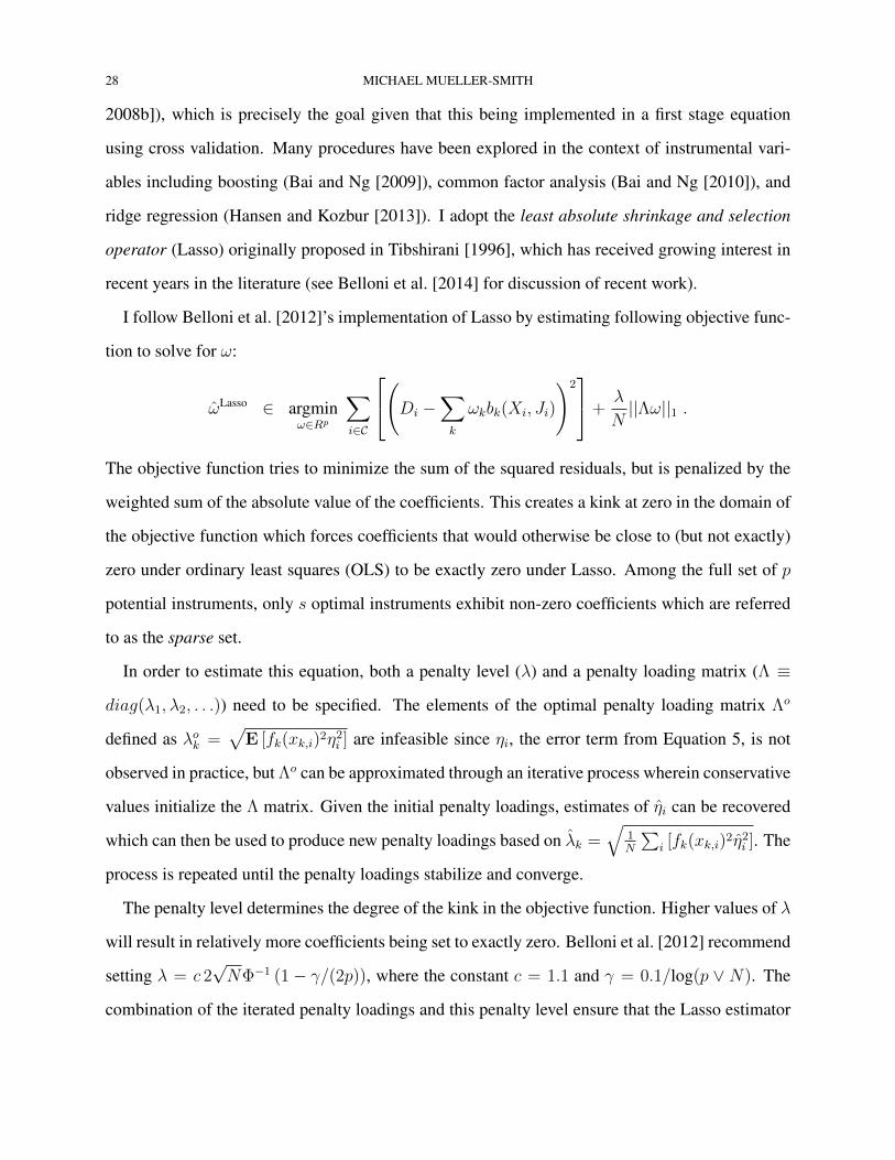
I follow Belloni et al. [2012]’s implementation of Lasso by estimating following objective func-
tion to solve for ω:
ωLasso ∈ argminω∈Rp
∑i∈C
(Di −∑k
ωkbk(Xi, Ji)
)2+
λ
N||Λω||1 .
The objective function tries to minimize the sum of the squared residuals, but is penalized by the
weighted sum of the absolute value of the coefficients. This creates a kink at zero in the domain of
the objective function which forces coefficients that would otherwise be close to (but not exactly)
zero under ordinary least squares (OLS) to be exactly zero under Lasso. Among the full set of p
potential instruments, only s optimal instruments exhibit non-zero coefficients which are referred
to as the sparse set.
In order to estimate this equation, both a penalty level (λ) and a penalty loading matrix (Λ ≡
diag(λ1, λ2, . . .)) need to be specified. The elements of the optimal penalty loading matrix Λo
defined as λok =√E [fk(xk,i)2η2i ] are infeasible since ηi, the error term from Equation 5, is not
observed in practice, but Λo can be approximated through an iterative process wherein conservative
values initialize the Λ matrix. Given the initial penalty loadings, estimates of ηi can be recovered
which can then be used to produce new penalty loadings based on λk =√
1N
∑i [fk(xk,i)
2η2i ]. The
process is repeated until the penalty loadings stabilize and converge.
The penalty level determines the degree of the kink in the objective function. Higher values of λ
will result in relatively more coefficients being set to exactly zero. Belloni et al. [2012] recommend
setting λ = c 2√NΦ−1 (1− γ/(2p)), where the constant c = 1.1 and γ = 0.1/log(p ∨ N). The
combination of the iterated penalty loadings and this penalty level ensure that the Lasso estimator
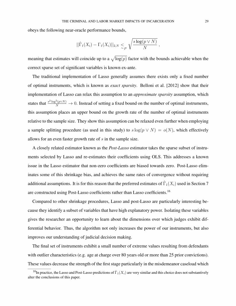
THE CRIMINAL AND LABOR MARKET IMPACTS OF INCARCERATION 29
obeys the following near-oracle performance bounds,
||Γ1(Xi)− Γ1(Xi)||2,N <∼P
√s log(p ∨N)
N,
meaning that estimates will coincide up to a√
log(p) factor with the bounds achievable when the
correct sparse set of significant variables is known ex-ante.
The traditional implementation of Lasso generally assumes there exists only a fixed number
of optimal instruments, which is known as exact sparsity. Belloni et al. [2012] show that their
implementation of Lasso can relax this assumption to an approximate sparsity assumption, which
states that s2 log2(p∨N)
N→ 0. Instead of setting a fixed bound on the number of optimal instruments,
this assumption places an upper bound on the growth rate of the number of optimal instruments
relative to the sample size. They show this assumption can be relaxed even further when employing
a sample splitting procedure (as used in this study) to s log(p ∨ N) = o(N), which effectively
allows for an even faster growth rate of s in the sample size.
A closely related estimator known as the Post-Lasso estimator takes the sparse subset of instru-
ments selected by Lasso and re-estimates their coefficients using OLS. This addresses a known
issue in the Lasso estimator that non-zero coefficients are biased towards zero. Post-Lasso elim-
inates some of this shrinkage bias, and achieves the same rates of convergence without requiring
additional assumptions. It is for this reason that the preferred estimates of Γ1(Xi) used in Section 7
are constructed using Post-Lasso coefficients rather than Lasso coefficients.16
Compared to other shrinkage procedures, Lasso and post-Lasso are particularly interesting be-
cause they identify a subset of variables that have high explanatory power. Isolating these variables
gives the researcher an opportunity to learn about the dimensions over which judges exhibit dif-
ferential behavior. Thus, the algorithm not only increases the power of our instruments, but also
improves our understanding of judicial decision making.
The final set of instruments exhibit a small number of extreme values resulting from defendants
with outlier characteristics (e.g. age at charge over 80 years old or more than 25 prior convictions).
These values decrease the strength of the first stage particularly in the misdemeanor caseload which16In practice, the Lasso and Post-Lasso predictions of Γ1(Xi) are very similar and this choice does not substantively
alter the conclusions of this paper.
30 MICHAEL MUELLER-SMITH
is relatively weaker overall. To deal with these observations, I winsorize the top and bottom 0.1
percentiles in the distribution of constructed instruments for the felony caseload and the top and
bottom 0.5 percentiles in the misdemeanor caseload.17 This adjustment has little to no impact
beyond improving precision of the estimates.
6. A PANEL MODEL OF THE IMPACT OF INCARCERATION
In contrast to existing work using judge randomization, this study adopts a panel framework to
estimate both the immediate and lasting effects of incarceration. Outcome Y for individual i, q
quarters after being charged at time t is modeled as a linear function of his incarceration status
and history, estimated court tendencies for non-focal sentencing outcomes (Dni ), and individual
characteristics (Xi). Incarceration status and history are formalized as three specific variables: (1)
the percent of days in a quarter that a defendant was incarcerated, (2) whether the defendant was
previously incarcerated if he is not currently incarcerated, and (3) the total amount of time the
defendant has spent incarcerated if he is not currently incarcerated. Quantifying these variables on
the quarterly versus monthly or weekly basis may introduce measurement error into the analysis;
this is unavoidable, however, as several outcome variables are only measured on the quarterly basis.
Because 60 to 70 percent of defendants are booked in county jail the week charges are filed
which generates a positive, mechanical correlation between incarceration status and criminal charges,
incarceration status in the days after charges are filed is recoded to zero until a new quarter has
started. This modification has minimal impacts on estimates for the felony caseload since incar-
ceration spells generally span several quarters if not years. It does however weaken the statistical
power of the research design in the misdemeanor caseload, as median incarceration length in this
context is no more than 10 days long.
To account for any unobserved changes based on the timing of defendant’s original charge or
the amount of follow-up time since the charge was filed, fixed effects µt and µq are also included.
17Trimming these observations was also pursued and generated similar results.
THE CRIMINAL AND LABOR MARKET IMPACTS OF INCARCERATION 31
This model is presented below:
Yi,t+q = δ1Incarceratedi,t+q + δ2Releasedi,t+q + δ3 (Releasedi,t+q × Exposurei,t+q) +(6)
δ4,qDni + δ5,qXi + µt + µq + ξi,t+q ,
where the primary variables of interest are defined as:
Incarceratedi,t+q =Days Incarceratedi,t+q
Days in Quartert+q,
Releasedi,t+q = 1
[T∑τ=1
Incarceratedi,t+q−τ > 0
]× 1 [Incarceratedi,t+q < 1] ,
Exposurei,t+q =
t+q∑ρ=1978q1
Incarceratedi,ρ .
To computeReleasedi,t+q, a maximum retrospective window (denoted by T ) is necessary. When a
more narrow window is used, δ2 and δ3 will capture primarily short-run effects. A longer window
will average short-run impacts with medium-term and long-term impacts. In order to strike a
balance between short and medium-run outcomes, I use 5 years as the maximum retrospective
window.
Total incarceration exposure is measured as the cumulative time spent incarcerated since the
first quarter of 1978, which is when the county jail and state prison data first begins. The model
only allows total exposure to impact outcomes once an inmate has been released in order to avoid
confounding the impact of duration after being released with any potential incapacitation effects.
Five years of post-charge outcomes are included in the panel data. In order to account for
repeated observations for the same defendant over time as well as the same defendant appearing in
the data for multiple charges, the standard errors are clustered at the defendant level.
The primary variables of interest will be instrumented using the methodology discussed in Sec-
tion 5. Because the data collected for this study spans 30 years of court filings, a time during which
some judges remain in office for over 20 years, the full set of instruments are recalculated every
32 MICHAEL MUELLER-SMITH
2 years over the range of t. This allows the estimated preferences of judges and assistant district
attorneys who remain in the court system for many years to change with time. Their relative pref-
erences will correspondingly adjust according to the court composition around the time charges
were filed (e.g. a “tough” judge becomes relatively less tough when all of the “easy” judges are
elected out of office and replaced with other “tough” judges).
Unlike fixed court outcomes such as guilt or fines, incarceration status and history change with
time. As a result, instruments for these variables must be recalculated each quarter since the
date of charge. This amounts to comparing the relative portion of each court’s caseload that is
incarcerated as of one quarter after charges were filed, two quarters after charges were filed and
so on. A benefit of recalculating the instruments over time in the panel framework is that the
estimation will leverage non-linear differences in the distribution of sentencing outcomes between
courtrooms rather than focus on average differences in overall sentence length. As an example,
some courts may be characterized by bimodal distributions of primarily short-term and long-term
incarceration, whereas others might utilize a more uniform distribution of sentences. While the
courts’ average sentence lengths might be equal, the realization of these sentences over time will
vary substantially.
7. THE CONTEMPORANEOUS AND POST-RELEASE EFFECTS OF INCARCERATION
This section presents the empirical findings of the study. It begins with a descriptive analysis
of how incarceration status, criminal activity and employment develop over time for defendants. I
then report several results to confirm the validity of the proposed research design. Finally, I present
the instrumental variable analysis which estimates the pre- and post-release effects of incarceration
on defendant and household outcomes. Particular attention is paid to distinguishing mechanisms
that underlie these results where possible. The results of my robustness exercises are discussed at
the end of the section.
Figure 3 shows the incarceration, criminal charge and employment rates of felony and misde-
meanor defendants relative to the timing of their criminal charges. Incarceration status, which is
separated out into being in county jail and state prison, as well as criminal charges are measured
THE CRIMINAL AND LABOR MARKET IMPACTS OF INCARCERATION 33
on a weekly basis, whereas employment is measured quarterly. In order to preserve the scale of
the figures, criminal charges in Week 0 are excluded since by definition all defendants would be
charged in this week.
In the run up to Week 0, there is a relative decline in the incarceration rate of both felony and mis-
demeanor defendants. This is mirrored by an increase in criminal activity. Once charges are filed,
there is an immediate increase in the likelihood of being jailed which is later displaced by prison
for felony defendants. These increases in incarceration coincide with a distinct drop in criminal
activity and employment. However, as inmates are released (months for felony defendants, weeks
for misdemeanor defendants), there appears to be a modest short-run increase in criminal activity
potentially upon release. In the 5 years of post-charge data, employment does not ever return to
pre-charge levels.
This study relies on the fact that defendants are randomly assigned to courtrooms. While there
is no reason to doubt the random assignment because it was implemented by an external office,
the fact that the data only includes non-sealed records means that the observed caseloads for each
courtroom may be censored in a non-random way. This can be tested by estimating the following
equation.
xi,t = α + τt + βCourti,t ⊗ τt + εi,t
In this equation, xi,t is a defendant covariate, Courti,t is a vector of court assignment dummy vari-
ables and τt is a vector of charge year dummy variables. Because Harris County introduced several
new courtrooms in response to growing caseloads over time, it is necessary to include time dum-
mies to absorb this variation. In addition, since the composition of courtroom actors (i.e. judge,
chief prosecutor, etc) is changing over time, I fully interact courtroom and year fixed effects so that
courtroom deviations are not arbitrarily constrained over time. In order to evaluate if the observed
caseloads are statistically equivalent, I conduct an F-test of the joint significance of β. This pro-
cedure can be repeated using a sentencing outcome instead of a defendant covariate to establish a
baseline of the instrument relevance if only using average differences between courtrooms.
Table 6 shows the results of this exercise. The first panel shows the F-tests for differences in
the balance of defendant covariates. The second panel shows the F-tests for differences in the
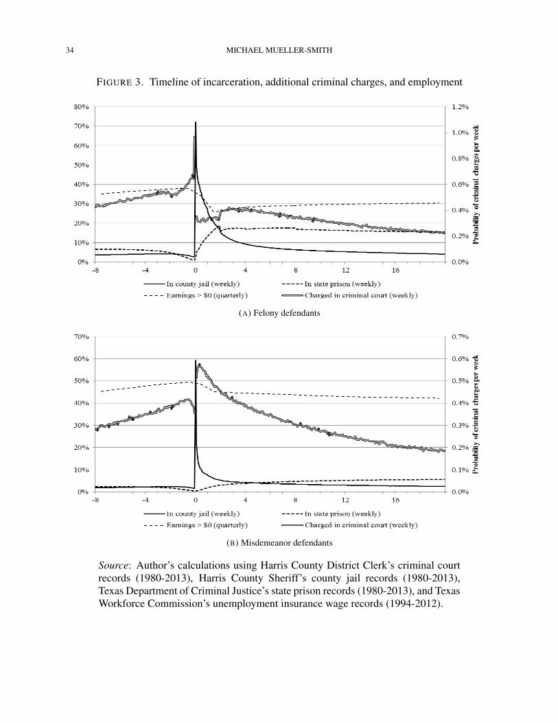
34 MICHAEL MUELLER-SMITH
FIGURE 3. Timeline of incarceration, additional criminal charges, and employment
(A) Felony defendants
(B) Misdemeanor defendants
Source: Author’s calculations using Harris County District Clerk’s criminal courtrecords (1980-2013), Harris County Sheriff’s county jail records (1980-2013),Texas Department of Criminal Justice’s state prison records (1980-2013), and TexasWorkforce Commission’s unemployment insurance wage records (1994-2012).
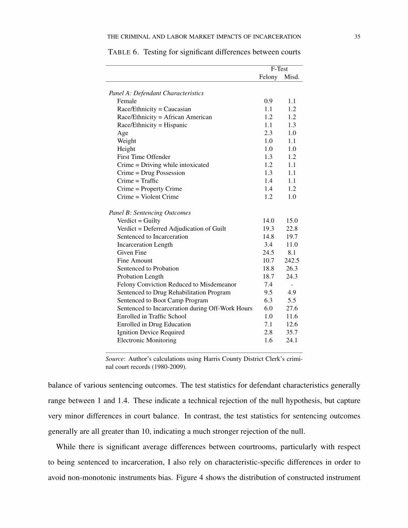
THE CRIMINAL AND LABOR MARKET IMPACTS OF INCARCERATION 35
TABLE 6. Testing for significant differences between courts
F-TestFelony Misd.
Panel A: Defendant CharacteristicsFemale 0.9 1.1Race/Ethnicity = Caucasian 1.1 1.2Race/Ethnicity = African American 1.2 1.2Race/Ethnicity = Hispanic 1.1 1.3Age 2.3 1.0Weight 1.0 1.1Height 1.0 1.0First Time Offender 1.3 1.2Crime = Driving while intoxicated 1.2 1.1Crime = Drug Possession 1.3 1.1Crime = Traffic 1.4 1.1Crime = Property Crime 1.4 1.2Crime = Violent Crime 1.2 1.0
Panel B: Sentencing OutcomesVerdict = Guilty 14.0 15.0Verdict = Deferred Adjudication of Guilt 19.3 22.8Sentenced to Incarceration 14.8 19.7Incarceration Length 3.4 11.0Given Fine 24.5 8.1Fine Amount 10.7 242.5Sentenced to Probation 18.8 26.3Probation Length 18.7 24.3Felony Conviction Reduced to Misdemeanor 7.4 -Sentenced to Drug Rehabilitation Program 9.5 4.9Sentenced to Boot Camp Program 6.3 5.5Sentenced to Incarceration during Off-Work Hours 6.0 27.6Enrolled in Traffic School 1.0 11.6Enrolled in Drug Education 7.1 12.6Ignition Device Required 2.8 35.7Electronic Monitoring 1.6 24.1
Source: Author’s calculations using Harris County District Clerk’s crimi-nal court records (1980-2009).
balance of various sentencing outcomes. The test statistics for defendant characteristics generally
range between 1 and 1.4. These indicate a technical rejection of the null hypothesis, but capture
very minor differences in court balance. In contrast, the test statistics for sentencing outcomes
generally are all greater than 10, indicating a much stronger rejection of the null.
While there is significant average differences between courtrooms, particularly with respect
to being sentenced to incarceration, I also rely on characteristic-specific differences in order to
avoid non-monotonic instruments bias. Figure 4 shows the distribution of constructed instrument
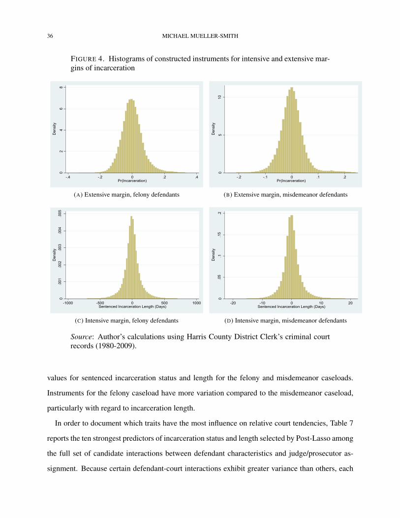
36 MICHAEL MUELLER-SMITH
FIGURE 4. Histograms of constructed instruments for intensive and extensive mar-gins of incarceration
02
46
8
Density
-.4 -.2 0 .2 .4Pr(Incarceration)
(A) Extensive margin, felony defendants
05
10Density
-.2 -.1 0 .1 .2Pr(Incarceration)
(B) Extensive margin, misdemeanor defendants
0.0
01.0
02.0
03.0
04.0
05D
ensi
ty
-1000 -500 0 500 1000Sentenced Incarceration Length (Days)
(C) Intensive margin, felony defendants
0.0
5.1
.15
.2D
ensi
ty
-20 -10 0 10 20Sentenced Incarceration Length (Days)
(D) Intensive margin, misdemeanor defendants
Source: Author’s calculations using Harris County District Clerk’s criminal courtrecords (1980-2009).
values for sentenced incarceration status and length for the felony and misdemeanor caseloads.
Instruments for the felony caseload have more variation compared to the misdemeanor caseload,
particularly with regard to incarceration length.
In order to document which traits have the most influence on relative court tendencies, Table 7
reports the ten strongest predictors of incarceration status and length selected by Post-Lasso among
the full set of candidate interactions between defendant characteristics and judge/prosecutor as-
signment. Because certain defendant-court interactions exhibit greater variance than others, each
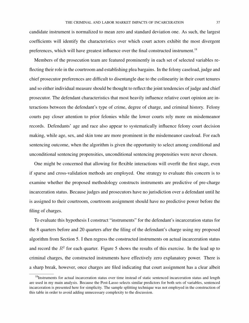
THE CRIMINAL AND LABOR MARKET IMPACTS OF INCARCERATION 37
candidate instrument is normalized to mean zero and standard deviation one. As such, the largest
coefficients will identify the characteristics over which court actors exhibit the most divergent
preferences, which will have greatest influence over the final constructed instrument.18
Members of the prosecution team are featured prominently in each set of selected variables re-
flecting their role in the courtroom and establishing plea bargains. In the felony caseload, judge and
chief prosecutor preferences are difficult to disentangle due to the colinearity in their court tenures
and so either individual measure should be thought to reflect the joint tendencies of judge and chief
prosecutor. The defendant characteristics that most heavily influence relative court opinion are in-
teractions between the defendant’s type of crime, degree of charge, and criminal history. Felony
courts pay closer attention to prior felonies while the lower courts rely more on misdemeanor
records. Defendants’ age and race also appear to systematically influence felony court decision
making, while age, sex, and skin tone are more prominent in the misdemeanor caseload. For each
sentencing outcome, when the algorithm is given the opportunity to select among conditional and
unconditional sentencing propensities, unconditional sentencing propensities were never chosen.
One might be concerned that allowing for flexible interactions will overfit the first stage, even
if sparse and cross-validation methods are employed. One strategy to evaluate this concern is to
examine whether the proposed methodology constructs instruments are predictive of pre-charge
incarceration status. Because judges and prosecutors have no jurisdiction over a defendant until he
is assigned to their courtroom, courtroom assignment should have no predictive power before the
filing of charges.
To evaluate this hypothesis I construct “instruments” for the defendant’s incarceration status for
the 8 quarters before and 20 quarters after the filing of the defendant’s charge using my proposed
algorithm from Section 5. I then regress the constructed instruments on actual incarceration status
and record the R2 for each quarter. Figure 5 shows the results of this exercise. In the lead up to
criminal charges, the constructed instruments have effectively zero explanatory power. There is
a sharp break, however, once charges are filed indicating that court assignment has a clear albeit
18Instruments for actual incarceration status over time instead of static sentenced incarceration status and lengthare used in my main analysis. Because the Post-Lasso selects similar predictors for both sets of variables, sentencedincarceration is presented here for simplicity. The sample splitting technique was not employed in the construction ofthis table in order to avoid adding unnecessary complexity to the discussion.
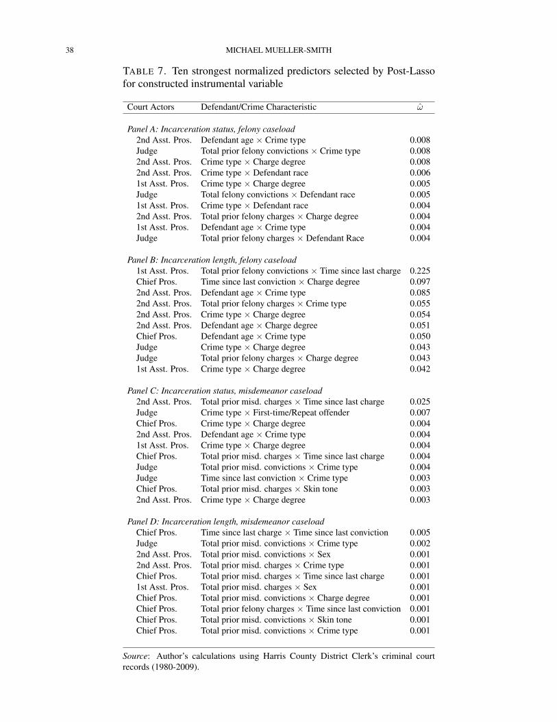
38 MICHAEL MUELLER-SMITH
TABLE 7. Ten strongest normalized predictors selected by Post-Lassofor constructed instrumental variable
Court Actors Defendant/Crime Characteristic ω
Panel A: Incarceration status, felony caseload2nd Asst. Pros. Defendant age × Crime type 0.008Judge Total prior felony convictions × Crime type 0.0082nd Asst. Pros. Crime type × Charge degree 0.0082nd Asst. Pros. Crime type × Defendant race 0.0061st Asst. Pros. Crime type × Charge degree 0.005Judge Total felony convictions × Defendant race 0.0051st Asst. Pros. Crime type × Defendant race 0.0042nd Asst. Pros. Total prior felony charges × Charge degree 0.0041st Asst. Pros. Defendant age × Crime type 0.004Judge Total prior felony charges × Defendant Race 0.004
Panel B: Incarceration length, felony caseload1st Asst. Pros. Total prior felony convictions × Time since last charge 0.225Chief Pros. Time since last conviction × Charge degree 0.0972nd Asst. Pros. Defendant age × Crime type 0.0852nd Asst. Pros. Total prior felony charges × Crime type 0.0552nd Asst. Pros. Crime type × Charge degree 0.0542nd Asst. Pros. Defendant age × Charge degree 0.051Chief Pros. Defendant age × Crime type 0.050Judge Crime type × Charge degree 0.043Judge Total prior felony charges × Charge degree 0.0431st Asst. Pros. Crime type × Charge degree 0.042
Panel C: Incarceration status, misdemeanor caseload2nd Asst. Pros. Total prior misd. charges × Time since last charge 0.025Judge Crime type × First-time/Repeat offender 0.007Chief Pros. Crime type × Charge degree 0.0042nd Asst. Pros. Defendant age × Crime type 0.0041st Asst. Pros. Crime type × Charge degree 0.004Chief Pros. Total prior misd. charges × Time since last charge 0.004Judge Total prior misd. convictions × Crime type 0.004Judge Time since last conviction × Crime type 0.003Chief Pros. Total prior misd. charges × Skin tone 0.0032nd Asst. Pros. Crime type × Charge degree 0.003
Panel D: Incarceration length, misdemeanor caseloadChief Pros. Time since last charge × Time since last conviction 0.005Judge Total prior misd. convictions × Crime type 0.0022nd Asst. Pros. Total prior misd. convictions × Sex 0.0012nd Asst. Pros. Total prior misd. charges × Crime type 0.001Chief Pros. Total prior misd. charges × Time since last charge 0.0011st Asst. Pros. Total prior misd. charges × Sex 0.001Chief Pros. Total prior misd. convictions × Charge degree 0.001Chief Pros. Total prior felony charges × Time since last conviction 0.001Chief Pros. Total prior misd. convictions × Skin tone 0.001Chief Pros. Total prior misd. convictions × Crime type 0.001
Source: Author’s calculations using Harris County District Clerk’s criminal courtrecords (1980-2009).
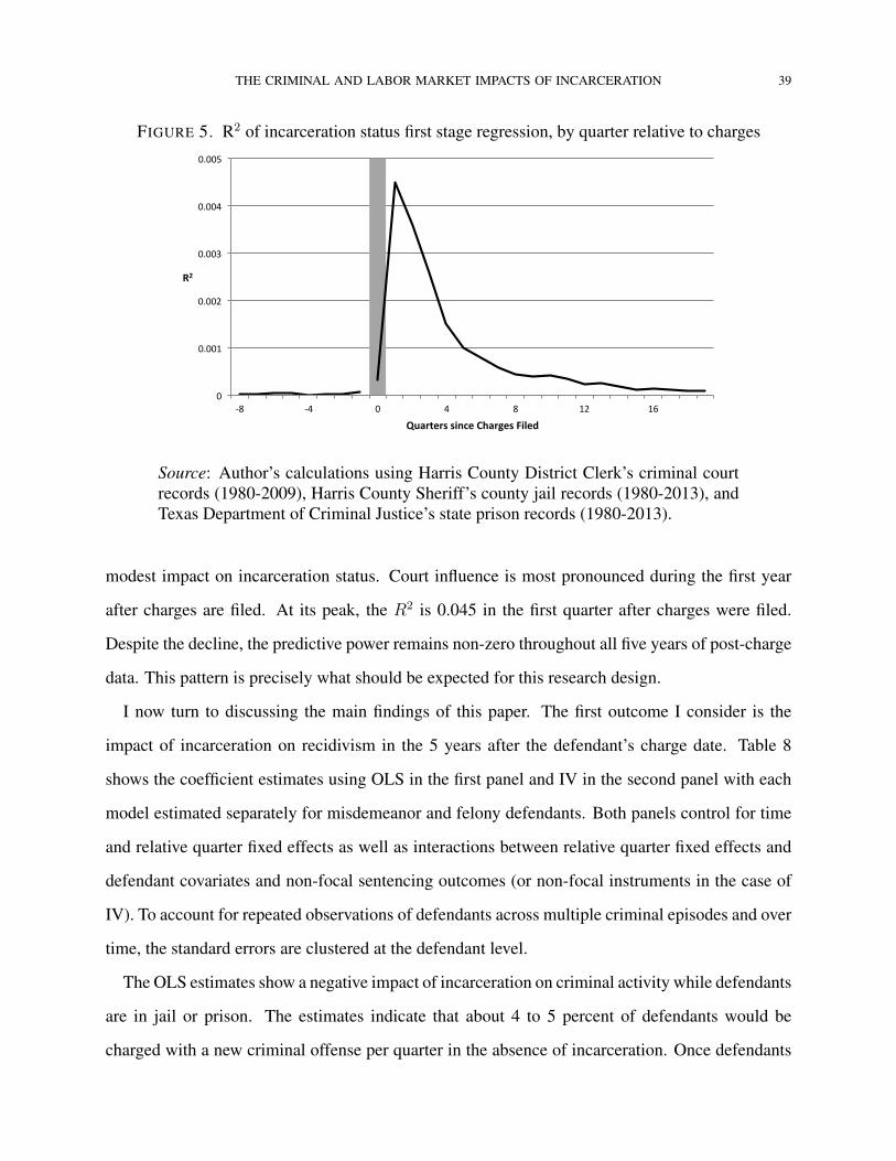
THE CRIMINAL AND LABOR MARKET IMPACTS OF INCARCERATION 39
FIGURE 5. R2 of incarceration status first stage regression, by quarter relative to charges
0
0.001
0.002
0.003
0.004
0.005
-‐8 -‐4 0 4 8 12 16
R2
Quarters since Charges Filed
Source: Author’s calculations using Harris County District Clerk’s criminal courtrecords (1980-2009), Harris County Sheriff’s county jail records (1980-2013), andTexas Department of Criminal Justice’s state prison records (1980-2013).
modest impact on incarceration status. Court influence is most pronounced during the first year
after charges are filed. At its peak, the R2 is 0.045 in the first quarter after charges were filed.
Despite the decline, the predictive power remains non-zero throughout all five years of post-charge
data. This pattern is precisely what should be expected for this research design.
I now turn to discussing the main findings of this paper. The first outcome I consider is the
impact of incarceration on recidivism in the 5 years after the defendant’s charge date. Table 8
shows the coefficient estimates using OLS in the first panel and IV in the second panel with each
model estimated separately for misdemeanor and felony defendants. Both panels control for time
and relative quarter fixed effects as well as interactions between relative quarter fixed effects and
defendant covariates and non-focal sentencing outcomes (or non-focal instruments in the case of
IV). To account for repeated observations of defendants across multiple criminal episodes and over
time, the standard errors are clustered at the defendant level.
The OLS estimates show a negative impact of incarceration on criminal activity while defendants
are in jail or prison. The estimates indicate that about 4 to 5 percent of defendants would be
charged with a new criminal offense per quarter in the absence of incarceration. Once defendants
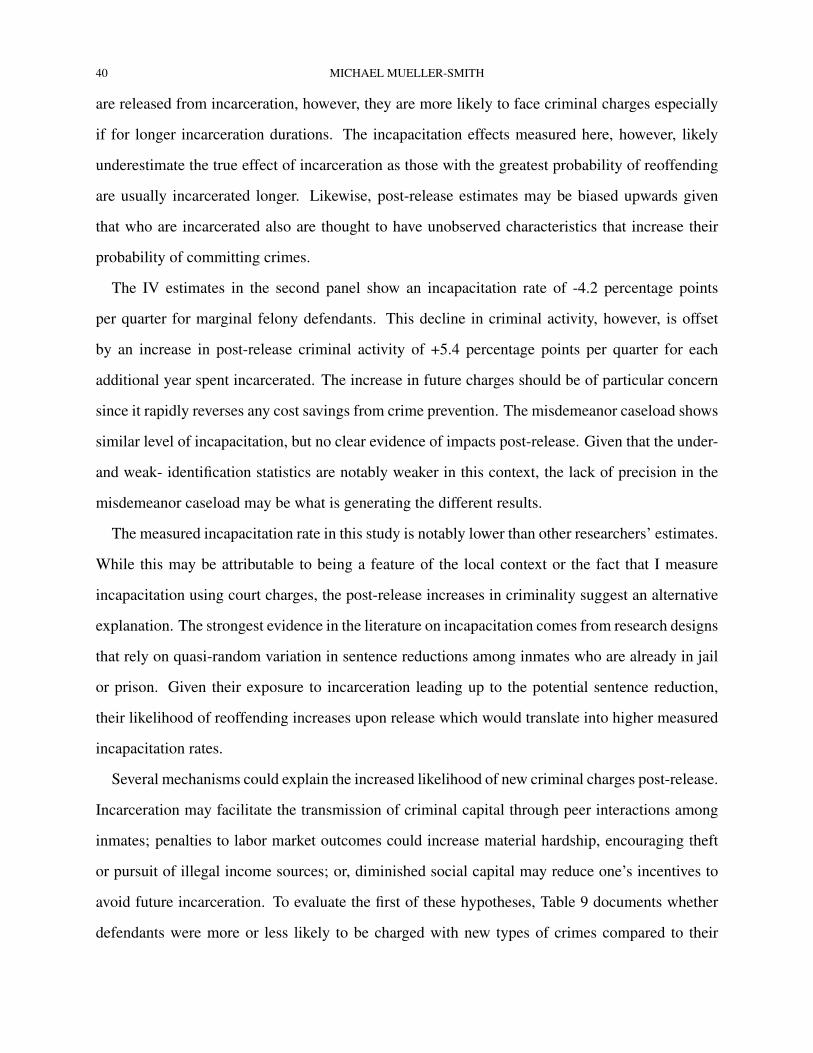
40 MICHAEL MUELLER-SMITH
are released from incarceration, however, they are more likely to face criminal charges especially
if for longer incarceration durations. The incapacitation effects measured here, however, likely
underestimate the true effect of incarceration as those with the greatest probability of reoffending
are usually incarcerated longer. Likewise, post-release estimates may be biased upwards given
that who are incarcerated also are thought to have unobserved characteristics that increase their
probability of committing crimes.
The IV estimates in the second panel show an incapacitation rate of -4.2 percentage points
per quarter for marginal felony defendants. This decline in criminal activity, however, is offset
by an increase in post-release criminal activity of +5.4 percentage points per quarter for each
additional year spent incarcerated. The increase in future charges should be of particular concern
since it rapidly reverses any cost savings from crime prevention. The misdemeanor caseload shows
similar level of incapacitation, but no clear evidence of impacts post-release. Given that the under-
and weak- identification statistics are notably weaker in this context, the lack of precision in the
misdemeanor caseload may be what is generating the different results.
The measured incapacitation rate in this study is notably lower than other researchers’ estimates.
While this may be attributable to being a feature of the local context or the fact that I measure
incapacitation using court charges, the post-release increases in criminality suggest an alternative
explanation. The strongest evidence in the literature on incapacitation comes from research designs
that rely on quasi-random variation in sentence reductions among inmates who are already in jail
or prison. Given their exposure to incarceration leading up to the potential sentence reduction,
their likelihood of reoffending increases upon release which would translate into higher measured
incapacitation rates.
Several mechanisms could explain the increased likelihood of new criminal charges post-release.
Incarceration may facilitate the transmission of criminal capital through peer interactions among
inmates; penalties to labor market outcomes could increase material hardship, encouraging theft
or pursuit of illegal income sources; or, diminished social capital may reduce one’s incentives to
avoid future incarceration. To evaluate the first of these hypotheses, Table 9 documents whether
defendants were more or less likely to be charged with new types of crimes compared to their
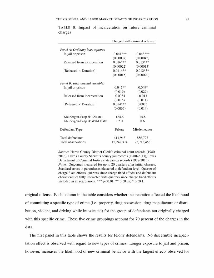
THE CRIMINAL AND LABOR MARKET IMPACTS OF INCARCERATION 41
TABLE 8. Impact of incarceration on future criminalcharges
Charged with criminal offense
Panel A: Ordinary least squaresIn jail or prison -0.041*** -0.048***
(0.00037) (0.00045)Released from incarceration 0.016*** 0.013***
(0.00022) (0.00013)[Released × Duration] 0.011*** 0.012***
(0.00015) (0.00020)
Panel B: Instrumental variablesIn jail or prison -0.042** -0.049*
(0.019) (0.029)Released from incarceration -0.0034 -0.013
(0.015) (0.011)[Released × Duration] 0.054*** 0.0075
(0.0065) (0.014)
Kleibergen-Paap rk LM stat. 184.6 25.8Kleibergen-Paap rk Wald F stat. 62.0 8.6
Defendant Type Felony Misdemeanor
Total defendants 411,943 856,727Total observations 12,242,374 25,718,458
Source: Harris County District Clerk’s criminal court records (1980-2013), Harris County Sheriff’s county jail records (1980-2013), TexasDepartment of Criminal Justice state prison records (1978-2013).Notes: Outcomes measured for up to 20 quarters after initial charges.Standard errors in parentheses clustered at defendant level. Quarter ofcharge fixed effects, quarters since charge fixed effects and defendantcharacteristics fully interacted with quarters since charge fixed effectsincluded in all regressions. *** p<0.01, ** p<0.05, * p<0.1.
original offense. Each column in the table considers whether incarceration affected the likelihood
of committing a specific type of crime (i.e. property, drug possession, drug manufacture or distri-
bution, violent, and driving while intoxicated) for the group of defendants not originally charged
with this specific crime. These five crime groupings account for 70 percent of the charges in the
data.
The first panel in this table shows the results for felony defendants. No discernible incapaci-
tation effect is observed with regard to new types of crimes. Longer exposure to jail and prison,
however, increases the likelihood of new criminal behavior with the largest effects observed for
42 MICHAEL MUELLER-SMITH
TABLE 9. Impact of incarceration on committing new types of offenses
Type of criminal offense: Property Drug poss. Drug mfr. or distr. Violent DWI
Panel A: Felony defendants, Instrumental variablesIn jail or prison 0.0056 -0.0100 -0.0050 -0.00067 -0.0040
(0.0087) (0.0077) (0.0035) (0.0050) (0.0035)Released from incarceration -0.0034 -0.0021 -0.0029 0.0039 -0.0025
(0.0075) (0.0063) (0.0025) (0.0038) (0.0032)[Released × Duration] 0.018*** 0.016*** 0.0044*** 0.0021 0.00041
(0.0035) (0.0042) (0.0014) (0.0016) (0.00077)
Kleibergen-Paap rk LM stat. 135.5 84.1 157.9 162.0 181.1Kleibergen-Paap rk Wald F stat. 45.4 28.1 53.0 54.3 60.8
Unique defendants 329,908 332,771 388,848 342,176 396,114Total observations 9,576,180 9,236,689 11,606,979 10,526,924 12,341,353
Panel B: Misdemeanor defendants, Instrumental variablesIn jail or prison -0.0085 0.011 0.0016 -0.010 -0.0067
(0.014) (0.013) (0.0059) (0.010) (0.0063)Released from incarceration 0.00011 0.0073* -0.0035* -0.0058* -0.0012
(0.0045) (0.0040) (0.0019) (0.0032) (0.0027)[Released × Duration] 0.0057 0.0012 0.0046 0.0031 -0.0039*
(0.0081) (0.0070) (0.0030) (0.0048) (0.0023)
Kleibergen-Paap rk LM stat. 17.0 21.0 26.0 21.1 27.7Kleibergen-Paap rk Wald F stat. 5.66 6.99 8.67 7.03 9.23
Unique defendants 721,929 787,623 852,817 797,154 645,724Total observations 21,763,728 23,77,3512 26,887,762 24,397,504 20,045,105
Source: Harris County District Clerk’s criminal court records (1980-2013), Harris County Sheriff’s county jailrecords (1980-2013), Texas Department of Criminal Justice state prison records (1978-2013).Notes: Each column excludes defendants originally charged with the type of crime being considered as the outcomevariable. Outcomes measured for up to 20 quarters after initial charges. Standard errors in parentheses clusteredat defendant level. Quarter of charge fixed effects, quarters since charge fixed effects and defendant characteris-tics fully interacted with quarters since charge fixed effects included in all regressions. *** p<0.01, ** p<0.05, *p<0.1.
drug possession and property crimes. While the increase in property crimes could be an indication
that incarceration impacts to income stability, the effect on drug offenses, which are the most com-
mon crime type among inmates, suggests a distinct possibility for criminal learning in this context.
Impacts on drug manufacture or distribution follow similar patterns.
The second panel shows the results for misdemeanor defendants. Like the felony context, mis-
demeanor defendants are more likely to be charged with drug possession post-release, even if their
prior offense did not relate to drug possession. The magnitude of this effect is smaller than the
felony context and is counter-balanced by declines in drug manufacture or distribution and violent
crimes.
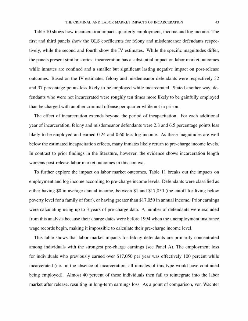
THE CRIMINAL AND LABOR MARKET IMPACTS OF INCARCERATION 43
Table 10 shows how incarceration impacts quarterly employment, income and log income. The
first and third panels show the OLS coefficients for felony and misdemeanor defendants respec-
tively, while the second and fourth show the IV estimates. While the specific magnitudes differ,
the panels present similar stories: incarceration has a substantial impact on labor market outcomes
while inmates are confined and a smaller but significant lasting negative impact on post-release
outcomes. Based on the IV estimates, felony and misdemeanor defendants were respectively 32
and 37 percentage points less likely to be employed while incarcerated. Stated another way, de-
fendants who were not incarcerated were roughly ten times more likely to be gainfully employed
than be charged with another criminal offense per quarter while not in prison.
The effect of incarceration extends beyond the period of incapacitation. For each additional
year of incarceration, felony and misdemeanor defendants were 2.8 and 6.5 percentage points less
likely to be employed and earned 0.24 and 0.60 less log income. As these magnitudes are well
below the estimated incapacitation effects, many inmates likely return to pre-charge income levels.
In contrast to prior findings in the literature, however, the evidence shows incarceration length
worsens post-release labor market outcomes in this context.
To further explore the impact on labor market outcomes, Table 11 breaks out the impacts on
employment and log income according to pre-charge income levels. Defendants were classified as
either having $0 in average annual income, between $1 and $17,050 (the cutoff for living below
poverty level for a family of four), or having greater than $17,050 in annual income. Prior earnings
were calculating using up to 3 years of pre-charge data. A number of defendants were excluded
from this analysis because their charge dates were before 1994 when the unemployment insurance
wage records begin, making it impossible to calculate their pre-charge income level.
This table shows that labor market impacts for felony defendants are primarily concentrated
among individuals with the strongest pre-charge earnings (see Panel A). The employment loss
for individuals who previously earned over $17,050 per year was effectively 100 percent while
incarcerated (i.e. in the absence of incarceration, all inmates of this type would have continued
being employed). Almost 40 percent of these individuals then fail to reintegrate into the labor
market after release, resulting in long-term earnings loss. As a point of comparison, von Wachter
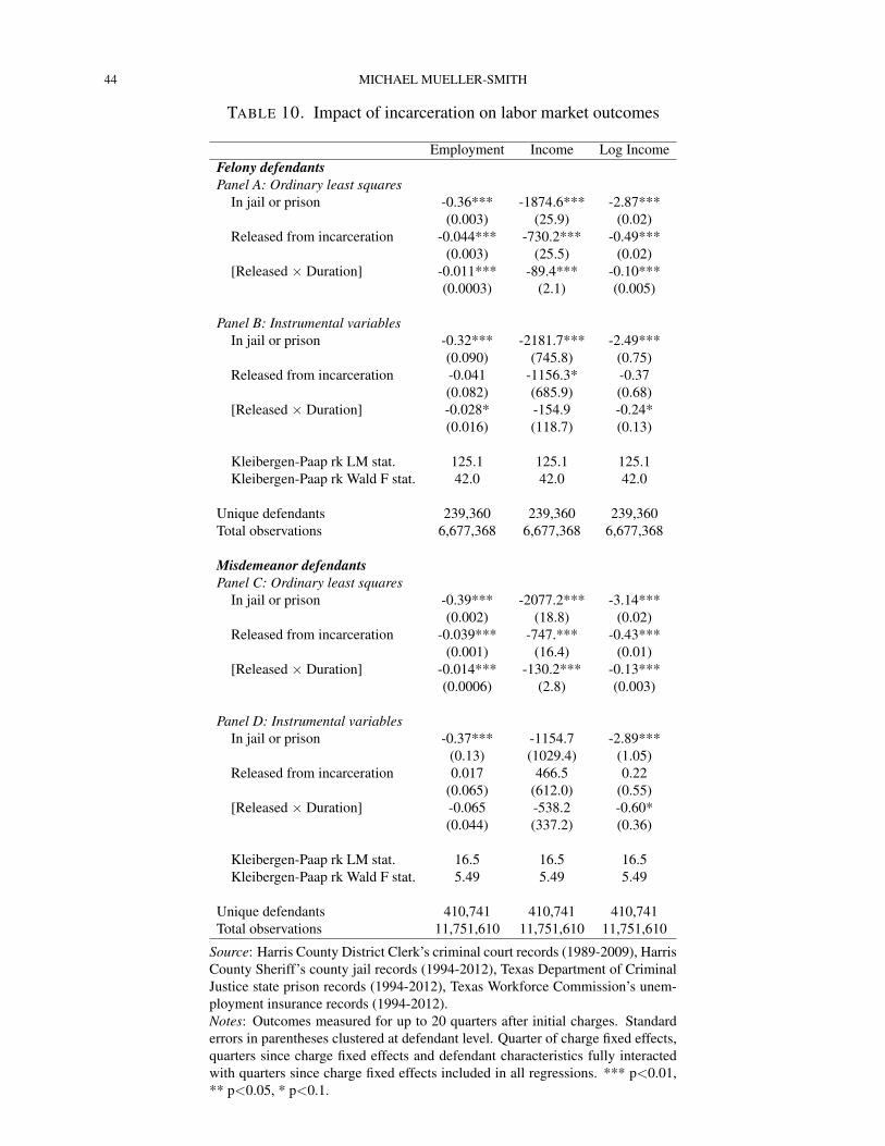
44 MICHAEL MUELLER-SMITH
TABLE 10. Impact of incarceration on labor market outcomes
Employment Income Log IncomeFelony defendantsPanel A: Ordinary least squares
In jail or prison -0.36*** -1874.6*** -2.87***(0.003) (25.9) (0.02)
Released from incarceration -0.044*** -730.2*** -0.49***(0.003) (25.5) (0.02)
[Released × Duration] -0.011*** -89.4*** -0.10***(0.0003) (2.1) (0.005)
Panel B: Instrumental variablesIn jail or prison -0.32*** -2181.7*** -2.49***
(0.090) (745.8) (0.75)Released from incarceration -0.041 -1156.3* -0.37
(0.082) (685.9) (0.68)[Released × Duration] -0.028* -154.9 -0.24*
(0.016) (118.7) (0.13)
Kleibergen-Paap rk LM stat. 125.1 125.1 125.1Kleibergen-Paap rk Wald F stat. 42.0 42.0 42.0
Unique defendants 239,360 239,360 239,360Total observations 6,677,368 6,677,368 6,677,368
Misdemeanor defendantsPanel C: Ordinary least squares
In jail or prison -0.39*** -2077.2*** -3.14***(0.002) (18.8) (0.02)
Released from incarceration -0.039*** -747.*** -0.43***(0.001) (16.4) (0.01)
[Released × Duration] -0.014*** -130.2*** -0.13***(0.0006) (2.8) (0.003)
Panel D: Instrumental variablesIn jail or prison -0.37*** -1154.7 -2.89***
(0.13) (1029.4) (1.05)Released from incarceration 0.017 466.5 0.22
(0.065) (612.0) (0.55)[Released × Duration] -0.065 -538.2 -0.60*
(0.044) (337.2) (0.36)
Kleibergen-Paap rk LM stat. 16.5 16.5 16.5Kleibergen-Paap rk Wald F stat. 5.49 5.49 5.49
Unique defendants 410,741 410,741 410,741Total observations 11,751,610 11,751,610 11,751,610
Source: Harris County District Clerk’s criminal court records (1989-2009), HarrisCounty Sheriff’s county jail records (1994-2012), Texas Department of CriminalJustice state prison records (1994-2012), Texas Workforce Commission’s unem-ployment insurance records (1994-2012).Notes: Outcomes measured for up to 20 quarters after initial charges. Standarderrors in parentheses clustered at defendant level. Quarter of charge fixed effects,quarters since charge fixed effects and defendant characteristics fully interactedwith quarters since charge fixed effects included in all regressions. *** p<0.01,** p<0.05, * p<0.1.
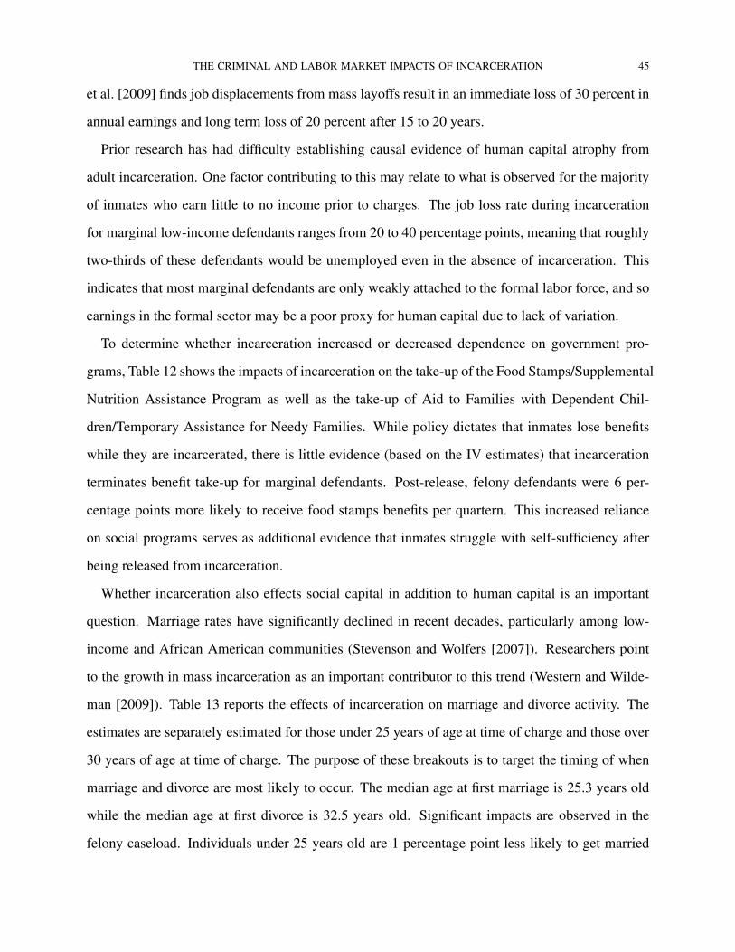
THE CRIMINAL AND LABOR MARKET IMPACTS OF INCARCERATION 45
et al. [2009] finds job displacements from mass layoffs result in an immediate loss of 30 percent in
annual earnings and long term loss of 20 percent after 15 to 20 years.
Prior research has had difficulty establishing causal evidence of human capital atrophy from
adult incarceration. One factor contributing to this may relate to what is observed for the majority
of inmates who earn little to no income prior to charges. The job loss rate during incarceration
for marginal low-income defendants ranges from 20 to 40 percentage points, meaning that roughly
two-thirds of these defendants would be unemployed even in the absence of incarceration. This
indicates that most marginal defendants are only weakly attached to the formal labor force, and so
earnings in the formal sector may be a poor proxy for human capital due to lack of variation.
To determine whether incarceration increased or decreased dependence on government pro-
grams, Table 12 shows the impacts of incarceration on the take-up of the Food Stamps/Supplemental
Nutrition Assistance Program as well as the take-up of Aid to Families with Dependent Chil-
dren/Temporary Assistance for Needy Families. While policy dictates that inmates lose benefits
while they are incarcerated, there is little evidence (based on the IV estimates) that incarceration
terminates benefit take-up for marginal defendants. Post-release, felony defendants were 6 per-
centage points more likely to receive food stamps benefits per quartern. This increased reliance
on social programs serves as additional evidence that inmates struggle with self-sufficiency after
being released from incarceration.
Whether incarceration also effects social capital in addition to human capital is an important
question. Marriage rates have significantly declined in recent decades, particularly among low-
income and African American communities (Stevenson and Wolfers [2007]). Researchers point
to the growth in mass incarceration as an important contributor to this trend (Western and Wilde-
man [2009]). Table 13 reports the effects of incarceration on marriage and divorce activity. The
estimates are separately estimated for those under 25 years of age at time of charge and those over
30 years of age at time of charge. The purpose of these breakouts is to target the timing of when
marriage and divorce are most likely to occur. The median age at first marriage is 25.3 years old
while the median age at first divorce is 32.5 years old. Significant impacts are observed in the
felony caseload. Individuals under 25 years old are 1 percentage point less likely to get married
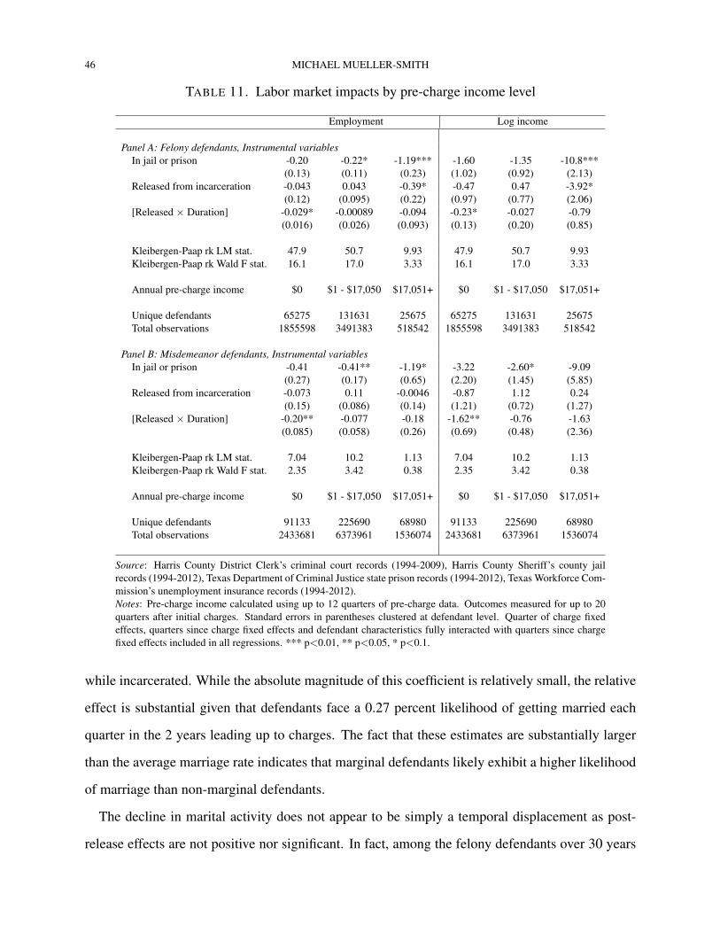
46 MICHAEL MUELLER-SMITH
TABLE 11. Labor market impacts by pre-charge income level
Employment Log income
Panel A: Felony defendants, Instrumental variablesIn jail or prison -0.20 -0.22* -1.19*** -1.60 -1.35 -10.8***
(0.13) (0.11) (0.23) (1.02) (0.92) (2.13)Released from incarceration -0.043 0.043 -0.39* -0.47 0.47 -3.92*
(0.12) (0.095) (0.22) (0.97) (0.77) (2.06)[Released × Duration] -0.029* -0.00089 -0.094 -0.23* -0.027 -0.79
(0.016) (0.026) (0.093) (0.13) (0.20) (0.85)
Kleibergen-Paap rk LM stat. 47.9 50.7 9.93 47.9 50.7 9.93Kleibergen-Paap rk Wald F stat. 16.1 17.0 3.33 16.1 17.0 3.33
Annual pre-charge income $0 $1 - $17,050 $17,051+ $0 $1 - $17,050 $17,051+
Unique defendants 65275 131631 25675 65275 131631 25675Total observations 1855598 3491383 518542 1855598 3491383 518542
Panel B: Misdemeanor defendants, Instrumental variablesIn jail or prison -0.41 -0.41** -1.19* -3.22 -2.60* -9.09
(0.27) (0.17) (0.65) (2.20) (1.45) (5.85)Released from incarceration -0.073 0.11 -0.0046 -0.87 1.12 0.24
(0.15) (0.086) (0.14) (1.21) (0.72) (1.27)[Released × Duration] -0.20** -0.077 -0.18 -1.62** -0.76 -1.63
(0.085) (0.058) (0.26) (0.69) (0.48) (2.36)
Kleibergen-Paap rk LM stat. 7.04 10.2 1.13 7.04 10.2 1.13Kleibergen-Paap rk Wald F stat. 2.35 3.42 0.38 2.35 3.42 0.38
Annual pre-charge income $0 $1 - $17,050 $17,051+ $0 $1 - $17,050 $17,051+
Unique defendants 91133 225690 68980 91133 225690 68980Total observations 2433681 6373961 1536074 2433681 6373961 1536074
Source: Harris County District Clerk’s criminal court records (1994-2009), Harris County Sheriff’s county jailrecords (1994-2012), Texas Department of Criminal Justice state prison records (1994-2012), Texas Workforce Com-mission’s unemployment insurance records (1994-2012).Notes: Pre-charge income calculated using up to 12 quarters of pre-charge data. Outcomes measured for up to 20quarters after initial charges. Standard errors in parentheses clustered at defendant level. Quarter of charge fixedeffects, quarters since charge fixed effects and defendant characteristics fully interacted with quarters since chargefixed effects included in all regressions. *** p<0.01, ** p<0.05, * p<0.1.
while incarcerated. While the absolute magnitude of this coefficient is relatively small, the relative
effect is substantial given that defendants face a 0.27 percent likelihood of getting married each
quarter in the 2 years leading up to charges. The fact that these estimates are substantially larger
than the average marriage rate indicates that marginal defendants likely exhibit a higher likelihood
of marriage than non-marginal defendants.
The decline in marital activity does not appear to be simply a temporal displacement as post-
release effects are not positive nor significant. In fact, among the felony defendants over 30 years
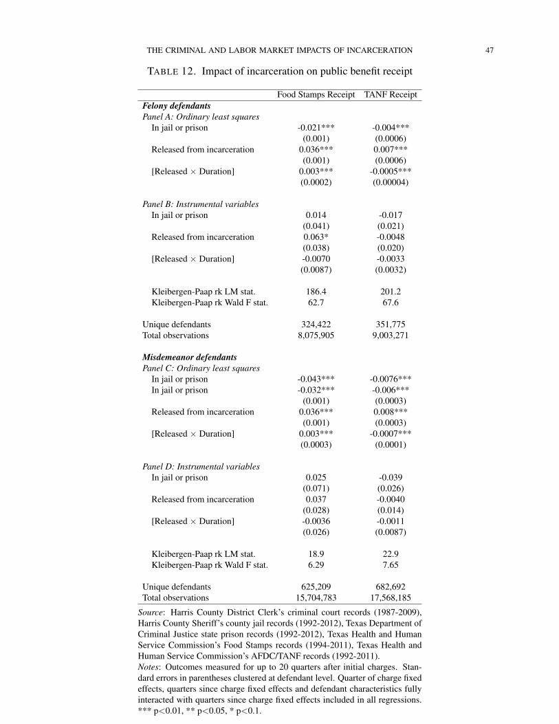
THE CRIMINAL AND LABOR MARKET IMPACTS OF INCARCERATION 47
TABLE 12. Impact of incarceration on public benefit receipt
Food Stamps Receipt TANF ReceiptFelony defendantsPanel A: Ordinary least squares
In jail or prison -0.021*** -0.004***(0.001) (0.0006)
Released from incarceration 0.036*** 0.007***(0.001) (0.0006)
[Released × Duration] 0.003*** -0.0005***(0.0002) (0.00004)
Panel B: Instrumental variablesIn jail or prison 0.014 -0.017
(0.041) (0.021)Released from incarceration 0.063* -0.0048
(0.038) (0.020)[Released × Duration] -0.0070 -0.0033
(0.0087) (0.0032)
Kleibergen-Paap rk LM stat. 186.4 201.2Kleibergen-Paap rk Wald F stat. 62.7 67.6
Unique defendants 324,422 351,775Total observations 8,075,905 9,003,271
Misdemeanor defendantsPanel C: Ordinary least squares
In jail or prison -0.043*** -0.0076***In jail or prison -0.032*** -0.006***
(0.001) (0.0003)Released from incarceration 0.036*** 0.008***
(0.001) (0.0003)[Released × Duration] 0.003*** -0.0007***
(0.0003) (0.0001)
Panel D: Instrumental variablesIn jail or prison 0.025 -0.039
(0.071) (0.026)Released from incarceration 0.037 -0.0040
(0.028) (0.014)[Released × Duration] -0.0036 -0.0011
(0.026) (0.0087)
Kleibergen-Paap rk LM stat. 18.9 22.9Kleibergen-Paap rk Wald F stat. 6.29 7.65
Unique defendants 625,209 682,692Total observations 15,704,783 17,568,185
Source: Harris County District Clerk’s criminal court records (1987-2009),Harris County Sheriff’s county jail records (1992-2012), Texas Department ofCriminal Justice state prison records (1992-2012), Texas Health and HumanService Commission’s Food Stamps records (1994-2011), Texas Health andHuman Service Commission’s AFDC/TANF records (1992-2011).Notes: Outcomes measured for up to 20 quarters after initial charges. Stan-dard errors in parentheses clustered at defendant level. Quarter of charge fixedeffects, quarters since charge fixed effects and defendant characteristics fullyinteracted with quarters since charge fixed effects included in all regressions.*** p<0.01, ** p<0.05, * p<0.1.
48 MICHAEL MUELLER-SMITH
old, who have the highest pre-charge marriage rate, the probability of divorce in a post-release
quarter increases by 0.13 percentage points for each year an inmate was incarcerated. This further
solidifies the argument that incarceration appears to play a causal role in preventing and dissolving
marriages.
Robustness Exercises. Several robustness exercises, which can be found in Appendix C, were
conducted to confirm the stability of the results. The results are generally robust, but some insta-
bility is observed in the incapacitation effects measured in the misdemeanor caseload. As such,
these results should be interpreted with caution.
In the first robustness check, I replicate the findings on criminal behavior using a statewide
criminal conviction database maintained by the Texas Department of Public Safety. It is known
that this database has incomplete coverage19, but is generally thought to capture the most serious
crimes. While I do not observe the incapacitation effects in this data, I do capture the increase
in criminality post-release for felony defendants. This ensures that this finding into the result of
differential intra-state mobility.
The second robustness exercise re-estimates my results using a more conservative level of clus-
tering: the court interacted with month of charge. Clustering at the defendant level accounts for
correlation in the error term between repeated observations in the panel, but fails to account for
correlation between defendants charged in the same courtroom. One example that could generate
this relationship is if defendants generate peer effects while in courtroom. Taking this conservative
approach, however, leaves my estimates virtually unchanged.
The third robustness check employs a two-step procedure wherein first stage residuals were
estimated using OLS and then used to construct a fourth order polynomial control function that
was added to outcome equation. The IV coefficients were then re-estimated using two-step GMM
to ensure the estimates were insensitive to potential misspecification in the first stage. The mag-
nitudes of the coefficients do not change noticeably and in fact the statistical precision in these
specifications generally improves.
19State auditors have generally found the submission rates from local authorities to the statewide repository to beroughly 60 to 70 percent over the years
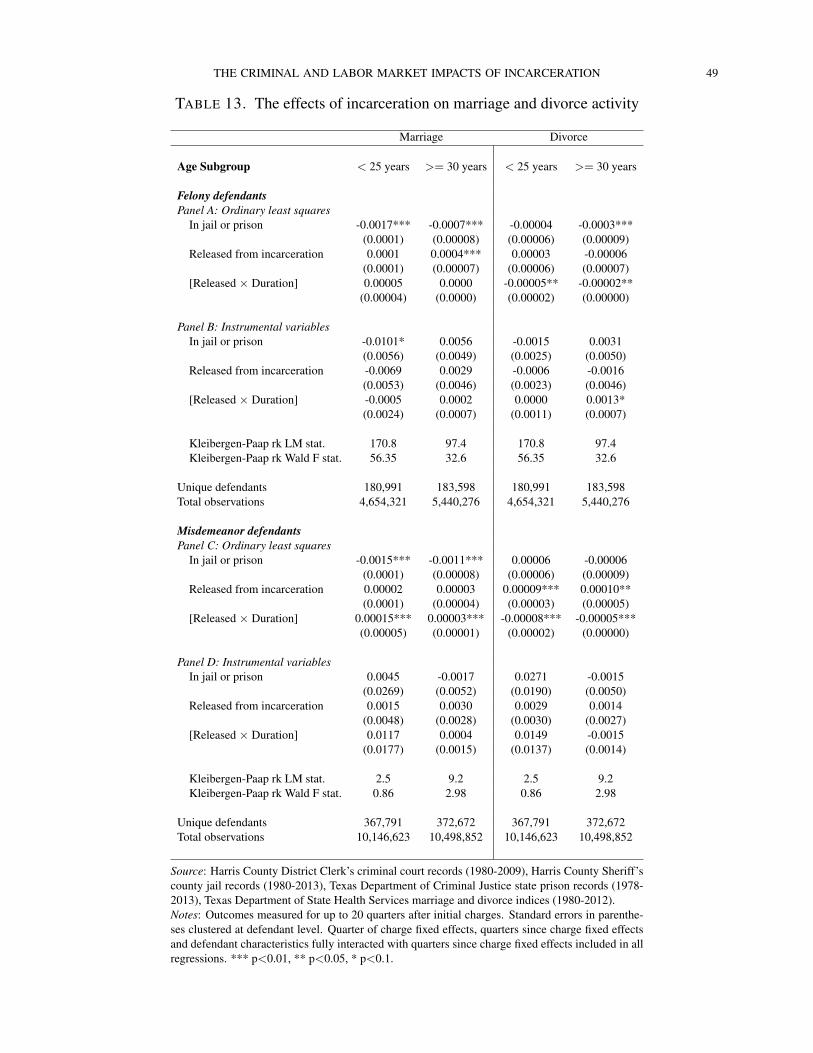
THE CRIMINAL AND LABOR MARKET IMPACTS OF INCARCERATION 49
TABLE 13. The effects of incarceration on marriage and divorce activity
Marriage Divorce
Age Subgroup < 25 years >= 30 years < 25 years >= 30 years
Felony defendantsPanel A: Ordinary least squares
In jail or prison -0.0017*** -0.0007*** -0.00004 -0.0003***(0.0001) (0.00008) (0.00006) (0.00009)
Released from incarceration 0.0001 0.0004*** 0.00003 -0.00006(0.0001) (0.00007) (0.00006) (0.00007)
[Released × Duration] 0.00005 0.0000 -0.00005** -0.00002**(0.00004) (0.0000) (0.00002) (0.00000)
Panel B: Instrumental variablesIn jail or prison -0.0101* 0.0056 -0.0015 0.0031
(0.0056) (0.0049) (0.0025) (0.0050)Released from incarceration -0.0069 0.0029 -0.0006 -0.0016
(0.0053) (0.0046) (0.0023) (0.0046)[Released × Duration] -0.0005 0.0002 0.0000 0.0013*
(0.0024) (0.0007) (0.0011) (0.0007)
Kleibergen-Paap rk LM stat. 170.8 97.4 170.8 97.4Kleibergen-Paap rk Wald F stat. 56.35 32.6 56.35 32.6
Unique defendants 180,991 183,598 180,991 183,598Total observations 4,654,321 5,440,276 4,654,321 5,440,276
Misdemeanor defendantsPanel C: Ordinary least squares
In jail or prison -0.0015*** -0.0011*** 0.00006 -0.00006(0.0001) (0.00008) (0.00006) (0.00009)
Released from incarceration 0.00002 0.00003 0.00009*** 0.00010**(0.0001) (0.00004) (0.00003) (0.00005)
[Released × Duration] 0.00015*** 0.00003*** -0.00008*** -0.00005***(0.00005) (0.00001) (0.00002) (0.00000)
Panel D: Instrumental variablesIn jail or prison 0.0045 -0.0017 0.0271 -0.0015
(0.0269) (0.0052) (0.0190) (0.0050)Released from incarceration 0.0015 0.0030 0.0029 0.0014
(0.0048) (0.0028) (0.0030) (0.0027)[Released × Duration] 0.0117 0.0004 0.0149 -0.0015
(0.0177) (0.0015) (0.0137) (0.0014)
Kleibergen-Paap rk LM stat. 2.5 9.2 2.5 9.2Kleibergen-Paap rk Wald F stat. 0.86 2.98 0.86 2.98
Unique defendants 367,791 372,672 367,791 372,672Total observations 10,146,623 10,498,852 10,146,623 10,498,852
Source: Harris County District Clerk’s criminal court records (1980-2009), Harris County Sheriff’scounty jail records (1980-2013), Texas Department of Criminal Justice state prison records (1978-2013), Texas Department of State Health Services marriage and divorce indices (1980-2012).Notes: Outcomes measured for up to 20 quarters after initial charges. Standard errors in parenthe-ses clustered at defendant level. Quarter of charge fixed effects, quarters since charge fixed effectsand defendant characteristics fully interacted with quarters since charge fixed effects included in allregressions. *** p<0.01, ** p<0.05, * p<0.1.
50 MICHAEL MUELLER-SMITH
The fourth exercise trimmed the top 99th and bottom 1st percentiles in the instrument values to
ensure that extreme values did not drive the results. I find the precision of the point estimates are
sensitive to the trimming exercise with some loss of significance on specific coefficients. This is
not surprising because I am eliminating variation. But taken as a whole, the general conclusions
appear qualitatively similar.
The fifth check replaces the Post-Lasso coefficients with Lasso coefficients to weight the basis
functions in the instrument construction. This should demonstrate that the results are not an ar-
bitrary artifact of the specific estimation process I used. What I find in this exercise is that the
estimates are very close together with similar magnitudes and precision, indicating that the Lasso
versus Post-Lasso distinction in this application is somewhat arbitrary.
The final robustness exercise drops the shrinkage procedure altogether and uses cross-validated
OLS to weight the basis functions. The first stage in this approach becomes weaker due to the
higher levels of noise in the generated instruments, which generates some movement in the IV
coefficients. The signs of my effects, however, are consistent with the main results.
8. REEXAMINING THE COSTS AND BENEFITS OF INCARCERATION
A common exercise when presented with incapacitation effects is to evaluate whether the cost
savings from crimes prevented outweigh the expense of keeping the inmate incarcerated (see Levitt
[1996] or Owens [2009]). Without taking into account general deterrence effects, this type of
calculation has been interpreted as a lower bound on the social gain from incarceration. But,
such an exercise is not necessarily so straightforward; Donohue III [2009] compiles a detailed
listing of additional mechanisms through which incarceration could impact welfare. At issue are
concerns regarding losses to inmate productivity, spillovers to household members, and impacts on
post-release behavior that could increase the overall costs. Many parameters needed for this more
detailed accounting have not been credibly estimated, and so attempts at evaluating this question
are either incomplete or rely heavily on assumptions.
The new estimates developed in this paper address some of the gaps in prior estimates. I cannot
conduct a full cost benefit analysis as my research design does not measure general deterrence
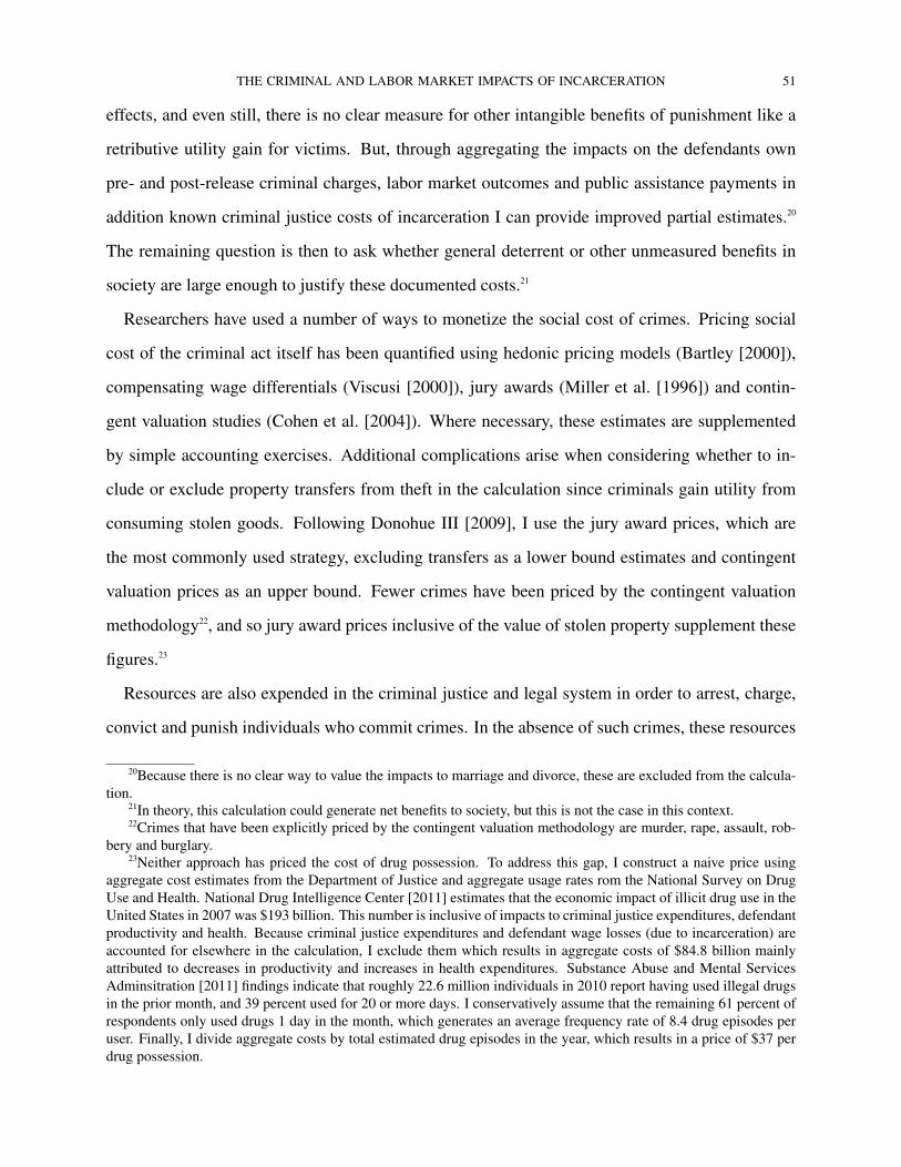
THE CRIMINAL AND LABOR MARKET IMPACTS OF INCARCERATION 51
effects, and even still, there is no clear measure for other intangible benefits of punishment like a
retributive utility gain for victims. But, through aggregating the impacts on the defendants own
pre- and post-release criminal charges, labor market outcomes and public assistance payments in
addition known criminal justice costs of incarceration I can provide improved partial estimates.20
The remaining question is then to ask whether general deterrent or other unmeasured benefits in
society are large enough to justify these documented costs.21
Researchers have used a number of ways to monetize the social cost of crimes. Pricing social
cost of the criminal act itself has been quantified using hedonic pricing models (Bartley [2000]),
compensating wage differentials (Viscusi [2000]), jury awards (Miller et al. [1996]) and contin-
gent valuation studies (Cohen et al. [2004]). Where necessary, these estimates are supplemented
by simple accounting exercises. Additional complications arise when considering whether to in-
clude or exclude property transfers from theft in the calculation since criminals gain utility from
consuming stolen goods. Following Donohue III [2009], I use the jury award prices, which are
the most commonly used strategy, excluding transfers as a lower bound estimates and contingent
valuation prices as an upper bound. Fewer crimes have been priced by the contingent valuation
methodology22, and so jury award prices inclusive of the value of stolen property supplement these
figures.23
Resources are also expended in the criminal justice and legal system in order to arrest, charge,
convict and punish individuals who commit crimes. In the absence of such crimes, these resources
20Because there is no clear way to value the impacts to marriage and divorce, these are excluded from the calcula-tion.
21In theory, this calculation could generate net benefits to society, but this is not the case in this context.22Crimes that have been explicitly priced by the contingent valuation methodology are murder, rape, assault, rob-
bery and burglary.23Neither approach has priced the cost of drug possession. To address this gap, I construct a naive price using
aggregate cost estimates from the Department of Justice and aggregate usage rates rom the National Survey on DrugUse and Health. National Drug Intelligence Center [2011] estimates that the economic impact of illicit drug use in theUnited States in 2007 was $193 billion. This number is inclusive of impacts to criminal justice expenditures, defendantproductivity and health. Because criminal justice expenditures and defendant wage losses (due to incarceration) areaccounted for elsewhere in the calculation, I exclude them which results in aggregate costs of $84.8 billion mainlyattributed to decreases in productivity and increases in health expenditures. Substance Abuse and Mental ServicesAdminsitration [2011] findings indicate that roughly 22.6 million individuals in 2010 report having used illegal drugsin the prior month, and 39 percent used for 20 or more days. I conservatively assume that the remaining 61 percent ofrespondents only used drugs 1 day in the month, which generates an average frequency rate of 8.4 drug episodes peruser. Finally, I divide aggregate costs by total estimated drug episodes in the year, which results in a price of $37 perdrug possession.
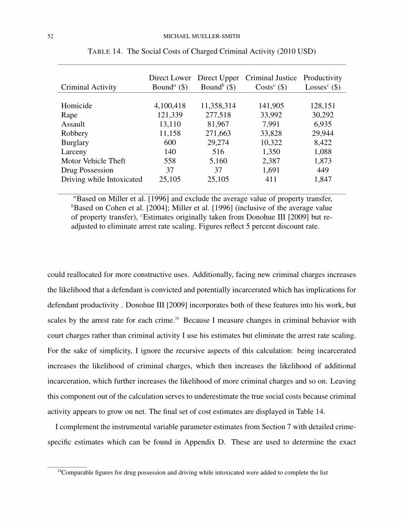
52 MICHAEL MUELLER-SMITH
TABLE 14. The Social Costs of Charged Criminal Activity (2010 USD)
Direct Lower Direct Upper Criminal Justice ProductivityCriminal Activity Bounda ($) Boundb ($) Costsc ($) Lossesc ($)
Homicide 4,100,418 11,358,314 141,905 128,151Rape 121,339 277,518 33,992 30,292Assault 13,110 81,967 7,991 6,935Robbery 11,158 271,663 33,828 29,944Burglary 600 29,274 10,322 8,422Larceny 140 516 1,350 1,088Motor Vehicle Theft 558 5,160 2,387 1,873Drug Possession 37 37 1,691 449Driving while Intoxicated 25,105 25,105 411 1,847
aBased on Miller et al. [1996] and exclude the average value of property transfer,bBased on Cohen et al. [2004]; Miller et al. [1996] (inclusive of the average valueof property transfer), cEstimates originally taken from Donohue III [2009] but re-adjusted to eliminate arrest rate scaling. Figures reflect 5 percent discount rate.
could reallocated for more constructive uses. Additionally, facing new criminal charges increases
the likelihood that a defendant is convicted and potentially incarcerated which has implications for
defendant productivity . Donohue III [2009] incorporates both of these features into his work, but
scales by the arrest rate for each crime.24 Because I measure changes in criminal behavior with
court charges rather than criminal activity I use his estimates but eliminate the arrest rate scaling.
For the sake of simplicity, I ignore the recursive aspects of this calculation: being incarcerated
increases the likelihood of criminal charges, which then increases the likelihood of additional
incarceration, which further increases the likelihood of more criminal charges and so on. Leaving
this component out of the calculation serves to underestimate the true social costs because criminal
activity appears to grow on net. The final set of cost estimates are displayed in Table 14.
I complement the instrumental variable parameter estimates from Section 7 with detailed crime-
specific estimates which can be found in Appendix D. These are used to determine the exact
24Comparable figures for drug possession and driving while intoxicated were added to complete the list
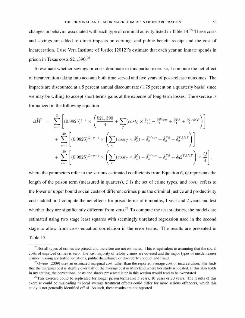
THE CRIMINAL AND LABOR MARKET IMPACTS OF INCARCERATION 53
changes in behavior associated with each type of criminal activity listed in Table 14.25 These costs
and savings are added to direct impacts on earnings and public benefit receipt and the cost of
incarceration. I use Vera Institute of Justice [2012]’s estimate that each year an inmate spends in
prison in Texas costs $21,390.26
To evaluate whether savings or costs dominate in this partial exercise, I compute the net effect
of incarceration taking into account both time served and five years of post-release outcomes. The
impacts are discounted at a 5 percent annual discount rate (1.75 percent on a quarterly basis) since
we may be willing to accept short-terms gains at the expense of long-term losses. The exercise is
formalized in the following equation
∆W =
Q∑q=1
[(0.9825)q−1 ×
($21, 390
4+∑C
(costC × δC1 )− δWage1 + δFS1 + δTANF1
)]
+20∑q=1
[(0.9825)Q+q−1 ×
(∑C
(costC × δC2 )− δWage2 + δFS2 + δTANF2
)]
+20∑q=1
[(0.9825)Q+q−1 ×
(∑C
(costC × δC3 )− δWage3 + δFS3 + δ32
TANF
)× Q
4
],
where the parameters refer to the various estimated coefficients from Equation 6, Q represents the
length of the prison term (measured in quarters), C is the set of crime types, and costC refers to
the lower or upper bound social costs of different crimes plus the criminal justice and productivity
costs added in. I compute the net effects for prison terms of 6 months, 1 year and 2 years and test
whether they are significantly different from zero.27 To compute the test statistics, the models are
estimated using two stage least squares with seemingly unrelated regression used in the second
stage to allow from cross-equation correlation in the error terms. The results are presented in
Table 15.
25Not all types of crimes are priced, and therefore are not estimated. This is equivalent to assuming that the socialcosts of unpriced crimes is zero. The vast majority of felony crimes are covered and the major types of misdemeanorcrimes missing are traffic violations, public disturbance or disorderly conduct and fraud.
26Owens [2009] uses an estimated marginal cost rather than the reported average cost of incarceration. She findsthat the marginal cost is slightly over half of the average cost in Maryland where her study is located. If this also holdsin my setting, the correctional costs and shares presented later in this section would tend to be overstated.
27This exercise could be replicated for longer prison terms like 5 years, 10 years or 20 years. The results of thisexercise could be misleading as local average treatment effects could differ for more serious offenders, which thisstudy is not generally identified off of. As such, these results are not reported.
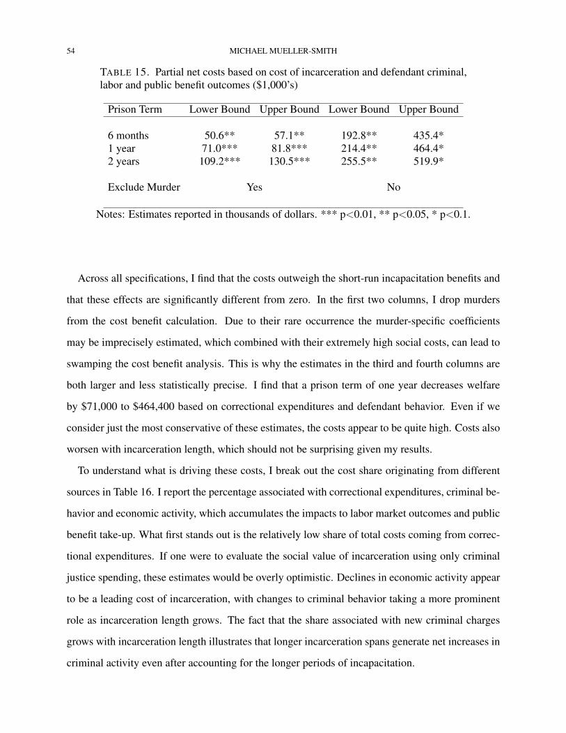
54 MICHAEL MUELLER-SMITH
TABLE 15. Partial net costs based on cost of incarceration and defendant criminal,labor and public benefit outcomes ($1,000’s)
Prison Term Lower Bound Upper Bound Lower Bound Upper Bound
6 months 50.6** 57.1** 192.8** 435.4*1 year 71.0*** 81.8*** 214.4** 464.4*2 years 109.2*** 130.5*** 255.5** 519.9*
Exclude Murder Yes No
Notes: Estimates reported in thousands of dollars. *** p<0.01, ** p<0.05, * p<0.1.
Across all specifications, I find that the costs outweigh the short-run incapacitation benefits and
that these effects are significantly different from zero. In the first two columns, I drop murders
from the cost benefit calculation. Due to their rare occurrence the murder-specific coefficients
may be imprecisely estimated, which combined with their extremely high social costs, can lead to
swamping the cost benefit analysis. This is why the estimates in the third and fourth columns are
both larger and less statistically precise. I find that a prison term of one year decreases welfare
by $71,000 to $464,400 based on correctional expenditures and defendant behavior. Even if we
consider just the most conservative of these estimates, the costs appear to be quite high. Costs also
worsen with incarceration length, which should not be surprising given my results.
To understand what is driving these costs, I break out the cost share originating from different
sources in Table 16. I report the percentage associated with correctional expenditures, criminal be-
havior and economic activity, which accumulates the impacts to labor market outcomes and public
benefit take-up. What first stands out is the relatively low share of total costs coming from correc-
tional expenditures. If one were to evaluate the social value of incarceration using only criminal
justice spending, these estimates would be overly optimistic. Declines in economic activity appear
to be a leading cost of incarceration, with changes to criminal behavior taking a more prominent
role as incarceration length grows. The fact that the share associated with new criminal charges
grows with incarceration length illustrates that longer incarceration spans generate net increases in
criminal activity even after accounting for the longer periods of incapacitation.
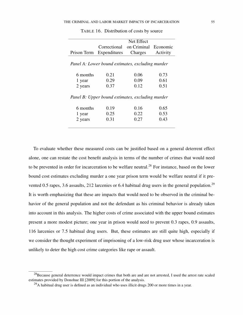
THE CRIMINAL AND LABOR MARKET IMPACTS OF INCARCERATION 55
TABLE 16. Distribution of costs by source
Net EffectCorrectional on Criminal Economic
Prison Term Expenditures Charges Activity
Panel A: Lower bound estimates, excluding murder
6 months 0.21 0.06 0.731 year 0.29 0.09 0.612 years 0.37 0.12 0.51
Panel B: Upper bound estimates, excluding murder
6 months 0.19 0.16 0.651 year 0.25 0.22 0.532 years 0.31 0.27 0.43
To evaluate whether these measured costs can be justified based on a general deterrent effect
alone, one can restate the cost benefit analysis in terms of the number of crimes that would need
to be prevented in order for incarceration to be welfare neutral.28 For instance, based on the lower
bound cost estimates excluding murder a one year prison term would be welfare neutral if it pre-
vented 0.5 rapes, 3.6 assaults, 212 larcenies or 6.4 habitual drug users in the general population.29
It is worth emphasizing that these are impacts that would need to be observed in the criminal be-
havior of the general population and not the defendant as his criminal behavior is already taken
into account in this analysis. The higher costs of crime associated with the upper bound estimates
present a more modest picture; one year in prison would need to prevent 0.3 rapes, 0.9 assaults,
116 larcenies or 7.5 habitual drug users. But, these estimates are still quite high, especially if
we consider the thought experiment of imprisoning of a low-risk drug user whose incarceration is
unlikely to deter the high cost crime categories like rape or assault.
28Because general deterrence would impact crimes that both are and are not arrested, I used the arrest rate scaledestimates provided by Donohue III [2009] for this portion of the analysis.
29A habitual drug user is defined as an individual who uses illicit drugs 200 or more times in a year.
56 MICHAEL MUELLER-SMITH
9. CONCLUSION
Criminal justice policy in the United States has grown increasingly reliant on incarceration in the
past three decades. Only in recent years has the incarcerated population begun to plateau. Previous
work showing substantial incapacitation gains has helped encourage this trend. The findings of this
study, however, should give pause to policy makers. Measured incapacitation rates in the context
of this study are quite low. This might be a function of the fact that I measure incapacitation using
court charges instead of criminal acts, which has led to lower estimates in other settings. But,
in spite of this caveat, I still find that incarceration led to increased criminality for inmates after
re-entry, which calls into question whether incapacitation is actually achieving true cost savings.
A number of non-crime outcomes are also negatively impacted by incarceration further dimin-
ishing its appeal. Effects on employment, earnings, benefit take-up and family formation indicate
that inmates face significant barriers to re-entry. Decreased economic self-sufficiency coincides
with greater use of government safety net programs. Lower marriage rates and increased divorce
rates indicate social isolation and raise important questions regarding potential spillovers to fami-
lies and communities.
This study cannot provide any evidence regarding potential general deterrent effects of incar-
ceration. However, based on the impacts to defendant outcomes, I estimate that incarceration
generates significant social costs to society. Unless the benefits of general deterrence are at the
upper bound of estimates found in the literature or there are other sizable intangible benefits to
incarceration, it is unlikely that incarceration for low-risk offenders in Texas is welfare improving.
LITERATURE CITED
D. S. Abrams, M. Bertrand, and S. Mullainathan. Do Judges Vary in Their Treatment of Race?
Journal of Legal Studies, 2010.
A. Aizer and J. Doyle. Juvenile incarceration and adult outcomes: Evidence from randomly-
assigned judges. NBER Working Paper, 2013.
J. Angrist and A. Krueger. Split-sample instrumental variables estimates of the return to schooling.
Journal of Business and Economic Statistics, 13(2):225–235, 1995.
J. Angrist, G. Imbens, and D. Rubin. Identification of causal effects using instrumental variables.
Journal of the American Statistical Association, 91(434):444–455, 1996.
D. Autor and S. Houseman. Do temporary-help jobs improve labor market outcomes for low-
skilled workers: Evidence from “work first”. American Economic Journal: Applied Economics,
2(3):96–128, 2010.
D. Autor, N. Maestas, K. Mullen, and A. Strand. Does delay cause decay? The effect of adminis-
trative decision time on the labor force participation and earnings of disability. 2013.
J. Bai and S. Ng. Selecting instrumental variables in a data rich environment. Journal of Time
Series Econometrics, 1(1), 2009.
J. Bai and S. Ng. Instrumental variable selection in a data rich environment. Econometric Theory,
26:1577–1606, 2010.
W. Bartley. Valuation of Specific Crime Rates: Summary. PhD thesis, Vanderbilt University, 2000.
P. Bayer, R. Hjalmarsson, and D. Pozen. Building criminal capital behind bars: Peer effects in
juvenile corrections. Quarterly Journal of Economics, 124(1):105–147, 2009.
A. Belloni, D. Chen, V. Chernozhukov, and C. Hansen. Sparse models and methods for optimal
instruments with an application to eminent domain. Econometrica, 80(6):2369–2429, 2012.
A. Belloni, V. Chernozhukov, and C. Hansen. High-dimensional methods and inference on struc-
tural and treatment effects. Journal of Economic Perspectives, 28(2):29–50, 2014.
S. Bright. Elected judges and the death penalty in texas: Why full habeas corpus review by inde-
pendent federal judges is indispensable to protecting constitutional rights. Tex. L. Rev., 78:1805,
2000.
58 MICHAEL MUELLER-SMITH
P. Buonanno and S. Raphael. Incarceration and Incapacitation: Evidence from the 2006 Italian
collective pardon. American Economic Review, 103(6):2437–2465, 2013.
Bureau of Justice Statistics. Justice expenditure and employment in the U.S., 1979. Technical
report, U.S. Department of Justice, Bureau of Justice Statistics, 1980.
S. Bushway. Labor market effects of permitting employer access to criminal history records.
Journal of Contemporary Criminal Justice, 20, 2004.
S. Bushway and E. Owens. Framing punishment: Incarceration, recommended sentences, and
recidivism. December 2012.
S. Bushway, E. Owens, and A. Piehl. Sentencing guidelines and judicial discretion: Quasi-
experimental evidence from human calculation errors. Journal of Empirical Legal Studies, 9
(2):291–319, 2012.
E. A. Carson. Imprisonment rate of sentenced prisoners under the jurisdiction of state or federal
correctional authorities per 100,000 U.S. residents, December 31, 1978-2012. National prisoner
statistics program, Bureau of Justice Statistics, 2013.
K. Chen and J. Shapiro. Do Harsher Prison Conditions Reduce Recidivism? A Discontinuity-
Based Approach. American Law and Economics Review, 9(1):1–29, 2007.
R. Cho and R. Lalonde. The impact of incarceration in state prison on the employment prospects
of women. IZA Discussion Paper No. 1792, 2005.
M. Cohen, R. Rust, S. Steen, and S. Tidd. Willingness to pay for crime control programs. Crimi-
nology, 42(1):86–109, 2004.
G. Dahl, A. Kostol, and M. Mogstad. Family welfare cultures. National Bureau of Economic
Research Working Paper 19237, 2013.
R. Di Tella and E. Schargrodsky. Do police reduce crime? Estimates using the allocation of police
forces after a terrorist attack. American Economic Review, 94(1):115–133, 2004.
J. Donohue III. Assessing the relative benefits of incarceration: Overall changes and the benefits
on the margin. In S. Raphael and M. Stoll, editors, Do Prisons Make Us Safer? Russell Sage
Foundation, 2009.
THE CRIMINAL AND LABOR MARKET IMPACTS OF INCARCERATION 59
J. Doyle. Child protection and child outcomes: Measuring the effects of foster care. American
Economic Review, 97(5):1583–1610, 2007.
J. Doyle. Child protection and adult crime: Using investigator assignment to estimate causal effects
of foster care. Journal of Political Economy, 116(4):746–770, 2008.
J. Doyle, J. Graves, J. Gruber, and S. Kleiner. Do high-cost hospitals deliver better care? Evidence
from ambulance referral patterns. National Bureau of Economic Research Working Paper 17936,
2012.
F. Drago and R. Galbiati. Indirect effects of a policy altering criminal behavior: Evidence from
the Italian prison experiment. American Economic Journal: Applied Economics, 4(2):199–218,
2012.
F. Drago, R. Galbiati, and P. Vertova. The deterrent effects of prison: Evidence from a natural
experiment. Journal of Political Economy, 117(2):257–280, 2009.
K. Finlay. Effect of employer access to criminal history data on the labor market outcomes of
ex-offenders and non-offenders. In D. Autor, editor, Studies of Labor Market Intermediation.
University of Chicago Press, 2009.
E. French and J. Song. The effect of disability insurance receipt on labor supply: A dynamic
analysis. Federal Reserve Bank of Chicago Working Paper 2012-12, 2012.
L. Glaze and E. Herberman. Correctional population in the united states, 2012. Technical report,
U.S. Department of Justice, Bureau of Justice Statistics, 2013.
D. Green and D. Winik. Using random judge assignments to estimate the effects of incarceration
and probation on recidivism among drug offenders. Criminology, 48(2):357–387, 2010.
J. Grogger. The effects of arrests on the employment and earnings of young men. Quarterly
Journal of Economics, 110:51–72, 1996.
C. Hansen and D. Kozbur. Instrumental variables estimation with many weak instruments using
regularized jive. 2013.
C. Hansen, J. Hausman, and W. Newey. Estimation with many instrumental variables. Journal of
Business and Economic Statistics, 26(4):398–422, 2008.
60 MICHAEL MUELLER-SMITH
T. Hastie, R. Tibshirani, and J. Friedman. The Elements of Statistical Learning: Data Mining,
Inference, and Prediction. Springer Series in Statistics, 2009.
J. Heckman and E. Vytlacil. Instrumental variables methods for the correlated random coefficient
model: Estimating the average rate of return to schooling when the return is correlated with
schooling. Journal of Human Resources, 33(4):974–987, 1998.
E. Helland and A. Tabarrok. Does three strickes deter? A nonparametric estimation. Journal of
Human Resources, 42(2):309–330, 2007.
G. Imbens and J. Angrist. Identification and estimation of local average treatment effects. Econo-
metrica, 62(2):467–475, 1994.
R. Johnson and S. Raphael. How much crime reduction does the maringal prison buy? Journal of
Law and Economics, 55(2):275–310, 2012.
L. Katz, S. Levitt, and E. Shustorovich. Prison conditions, capital punishment, and deterrence.
American Law and Economics Review, 5(2):318–343, 2003.
N. Kauder and B. Ostrom. State sentencing guidelines: Profiles and continuum. Technical report,
National Center for State Courts, 2008.
J. Kling. Incarceration length, employment and earnings. American Economic Review, 96(3):
863–876, 2006.
E. Korn and S. Baumrind. Clinician preferences and the estimation of causal treatment differences.
Statistical Science, 13(3):209–235, 1998.
E. Korn, D. Teeter, and S. Baumrind. Using explicit clinician preferences in nonrandomized study
designs. Journal of statistical planning and inference, 96(1):67–82, 2001.
I. Kuziemko. Should prisoners be released via rules or discretion? Quarterly Journal of Econom-
ics, 128(1):371–424, 2013.
T. Kyckelhahn. Justice expenditure and employment extracts, 2010 - preliminary. Technical report,
U.S. Department of Justice, Bureau of Justice Statistics, 2013.
D. Lee and J. McCrary. The deterrence effect of prison: Dynamic theory and evidence. unpublished
manuscript, 2009.
THE CRIMINAL AND LABOR MARKET IMPACTS OF INCARCERATION 61
H. Leeb and B. M. Potscher. Can one estimate the unconditional distribution of post-model-
selection estimators? Econometric Theory, 24(2):338–76, 2008.
S. Levitt. The effect of prison population size on crime rates: Evidence from prison overcrowding
litigation. Quarterly Journal of Economics, 111(2):319–351, 1996.
R. Liedka, A. Piehl, and B. Useem. The crime-control effect of incarceration: Does scale matter?
Criminology and Public Policy, 5(2):245–276, 2006.
J. Ludwig and J. Kling. Is crime contagious? Journal of Law and Economics, 50(3):491–518,
August 2007.
N. Maestas, K. Mullen, and A. Strand. Does disability insurance receipt discourage work? Using
examiner assignment to estimate causal effects of SSDI receipt. American Economic Review,
103(5):1797–1829, 2013.
E. Maurin and A. Ouss. Sentence reductions and recidivism: Lessons from the Bastille day quasi
experiment. IZA Discussion Papers 3990, 2009.
J. McCrary and S. Sanga. Youth offenders and the deterrence effect of prison. unpublished manu-
script, 2012.
T. Miller, M. Cohen, and B. Wiersema. Victim costs and consequences: A new look. National
institute of justice research report, ncj-155282, U.S. Department of Justice, 1996.
D. Munroe and L. Wilse-Samson. Measuring local externalities of home foreclosures. unpublished
manuscript, 2012.
D. Nagin and M. G. Snodgrass. The effect of incarceration on re-offending: Evidence from a
natural experiment in Pennsylvania. Journal of Quantitative Criminology, 29(4):601–642, 2013.
National Drug Intelligence Center. The economic impact of illicit drug use on american society.
Technical report, U.S. Department of Justice, 2011.
A. Ouss. Prison as a school of crime: Evidence from cell-level interaction. 2013.
E. Owens. More time, less crime? Estimating the incapacitative effect of sentence enhancements.
Journal of Law and Economics, 52(3):551–579, 2009.
D. Pager. The mark of a criminal record. American Journal of Sociology, 108:937–975, 2003.
62 MICHAEL MUELLER-SMITH
B. Pettit and C. Lyons. Status and the stigma of incarceration: The labor market effects by race,
class and criminal involvement. In S. Bushway, M. Stoll, and david weiman, editors, Barriers
to Reentry? The Labor Market for Released Prisoners in Post-Industrial America. Russell Sage
Foundation, 2007.
J. Price and J. Wolfers. Racial Discrimination Among NBA Referees. Quarterly Journal of Eco-
nomics, 125(4):1859–1887, 2010.
S. Raphael. Early incarceration spells and the transition to adulthood. In S. Bushway, M. Stoll,
and david weiman, editors, Barriers to Reentry? The Labor Market for Released Prisoners in
Post-Industrial America. Russell Sage Foundation, 2007.
S. Rimer and R. Bonner. Texas lawyer’s death row record a concern. New York Times, June 11,
2000.
W. Sabol. Local labor market conditions and post-prison employment experience of offenders
released from ohio prisons. In S. Bushway, M. Stoll, and david weiman, editors, Barriers to
Reentry? The Labor Market for Released Prisoners in Post-Industrial America. Russell Sage
Foundation, 2007.
B. Stevenson and J. Wolfers. Marriage and divorce: Changes and their driving forces. Journal of
Economic Perspectives, 21(2):27–52, 2007.
Substance Abuse and Mental Services Adminsitration. Results from the 2010 national survey on
drug use and health: Summary of national findings. Technical report, U.S. Department of Health
and Human Services, 2011.
Texas Code of Criminal Procedure. URL http://www.statutes.legis.state.tx.us/
Docs/SDocs/CODEOFCRIMINALPROCEDURE.pdf. Accessed on March 31, 2014.
R. Tibshirani. Regression shrinkage and selection via the lasso. Journal of the Royal Statistical
Society, 58(1):267–288, 1996.
Vera Institute of Justice. The price of prisons: What incarceration costs taxpayers. Technical
report, Center on Sentencing and Corrections, 2012.
W. K. Viscusi. The value of life in legal context: Survey and critique. American Law and Eco-
nomics Review, 2:195–222, 2000.
T. von Wachter, J. Song, and J. Manchester. Long-term earnings losses due to mass layoffs during
the 1982 recession: An analysis using u.s. administrative data from 1974 to 2004. April 2009.
J. Waldfogel. Does inter-judge disparity justify empirically based sentencing guidelines? Interna-
tional Review of Law and Economics, 18(3):293–304, 1998.
R. Walmsley. World Prison Population List (8th edition). International Centre for Prison Studies,
2009.
B. Western. Punishment and Inequality in America. Russell Sage Foundation, 2006.
B. Western and C. Wildeman. The black family and mass incarceration. The ANNALS of the
American Academy of Politcal and Social Science, 621:221–242, January 2009.
J. M. Wooldridge. On two stage least squares estimation of the average treatment effect in a random
coefficient model. Economics Letters, 56(2):129–133, 1997.
J. M. Wooldridge. Further results on instrumental variables estimation of average treatment effects
in the correlated random coefficient model. Economics Letters, 79(2):185–191, 2003.
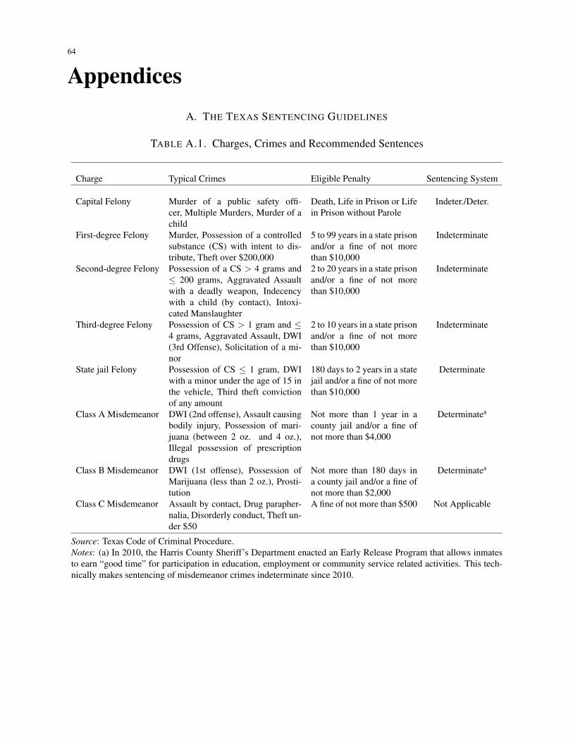
64
AppendicesA. THE TEXAS SENTENCING GUIDELINES
TABLE A.1. Charges, Crimes and Recommended Sentences
Charge Typical Crimes Eligible Penalty Sentencing System
Capital Felony Murder of a public safety offi-cer, Multiple Murders, Murder of achild
Death, Life in Prison or Lifein Prison without Parole
Indeter./Deter.
First-degree Felony Murder, Possession of a controlledsubstance (CS) with intent to dis-tribute, Theft over $200,000
5 to 99 years in a state prisonand/or a fine of not morethan $10,000
Indeterminate
Second-degree Felony Possession of a CS > 4 grams and≤ 200 grams, Aggravated Assaultwith a deadly weapon, Indecencywith a child (by contact), Intoxi-cated Manslaughter
2 to 20 years in a state prisonand/or a fine of not morethan $10,000
Indeterminate
Third-degree Felony Possession of CS > 1 gram and ≤4 grams, Aggravated Assault, DWI(3rd Offense), Solicitation of a mi-nor
2 to 10 years in a state prisonand/or a fine of not morethan $10,000
Indeterminate
State jail Felony Possession of CS ≤ 1 gram, DWIwith a minor under the age of 15 inthe vehicle, Third theft convictionof any amount
180 days to 2 years in a statejail and/or a fine of not morethan $10,000
Determinate
Class A Misdemeanor DWI (2nd offense), Assault causingbodily injury, Possession of mari-juana (between 2 oz. and 4 oz.),Illegal possession of prescriptiondrugs
Not more than 1 year in acounty jail and/or a fine ofnot more than $4,000
Determinatea
Class B Misdemeanor DWI (1st offense), Possession ofMarijuana (less than 2 oz.), Prosti-tution
Not more than 180 days ina county jail and/or a fine ofnot more than $2,000
Determinatea
Class C Misdemeanor Assault by contact, Drug parapher-nalia, Disorderly conduct, Theft un-der $50
A fine of not more than $500 Not Applicable
Source: Texas Code of Criminal Procedure.Notes: (a) In 2010, the Harris County Sheriff’s Department enacted an Early Release Program that allows inmatesto earn “good time” for participation in education, employment or community service related activities. This tech-nically makes sentencing of misdemeanor crimes indeterminate since 2010.
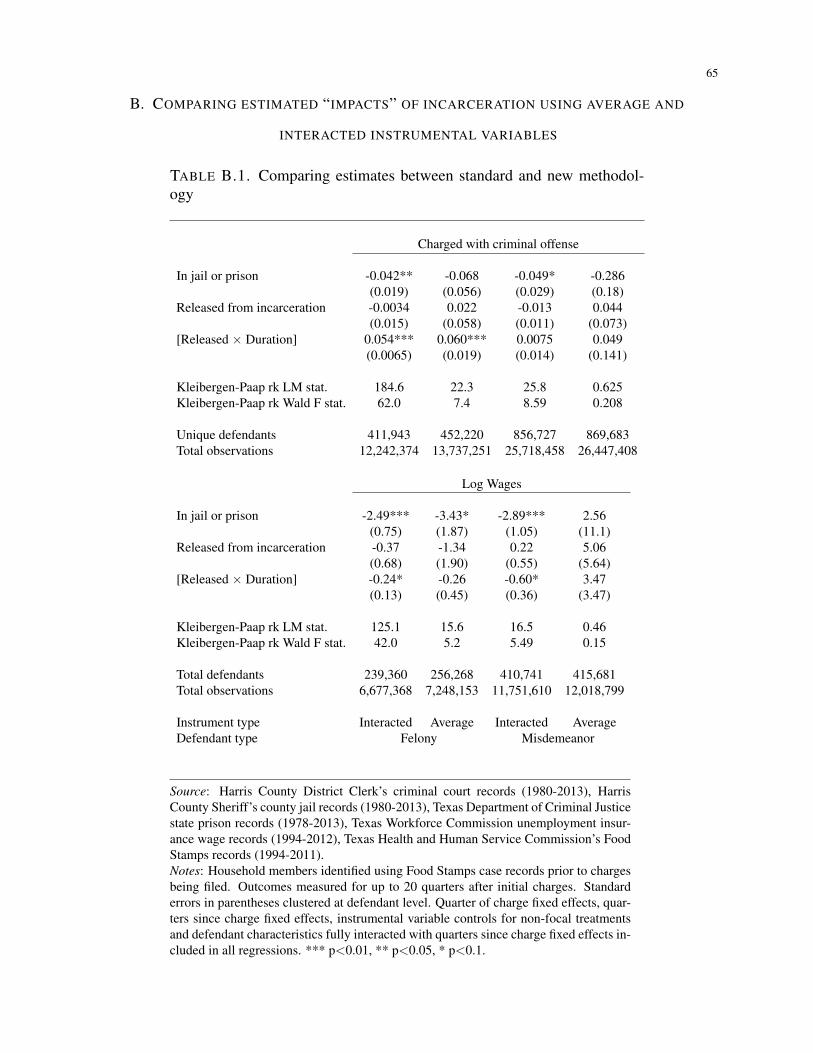
65
B. COMPARING ESTIMATED “IMPACTS” OF INCARCERATION USING AVERAGE AND
INTERACTED INSTRUMENTAL VARIABLES
TABLE B.1. Comparing estimates between standard and new methodol-ogy
Charged with criminal offense
In jail or prison -0.042** -0.068 -0.049* -0.286(0.019) (0.056) (0.029) (0.18)
Released from incarceration -0.0034 0.022 -0.013 0.044(0.015) (0.058) (0.011) (0.073)
[Released × Duration] 0.054*** 0.060*** 0.0075 0.049(0.0065) (0.019) (0.014) (0.141)
Kleibergen-Paap rk LM stat. 184.6 22.3 25.8 0.625Kleibergen-Paap rk Wald F stat. 62.0 7.4 8.59 0.208
Unique defendants 411,943 452,220 856,727 869,683Total observations 12,242,374 13,737,251 25,718,458 26,447,408
Log Wages
In jail or prison -2.49*** -3.43* -2.89*** 2.56(0.75) (1.87) (1.05) (11.1)
Released from incarceration -0.37 -1.34 0.22 5.06(0.68) (1.90) (0.55) (5.64)
[Released × Duration] -0.24* -0.26 -0.60* 3.47(0.13) (0.45) (0.36) (3.47)
Kleibergen-Paap rk LM stat. 125.1 15.6 16.5 0.46Kleibergen-Paap rk Wald F stat. 42.0 5.2 5.49 0.15
Total defendants 239,360 256,268 410,741 415,681Total observations 6,677,368 7,248,153 11,751,610 12,018,799
Instrument type Interacted Average Interacted AverageDefendant type Felony Misdemeanor
Source: Harris County District Clerk’s criminal court records (1980-2013), HarrisCounty Sheriff’s county jail records (1980-2013), Texas Department of Criminal Justicestate prison records (1978-2013), Texas Workforce Commission unemployment insur-ance wage records (1994-2012), Texas Health and Human Service Commission’s FoodStamps records (1994-2011).Notes: Household members identified using Food Stamps case records prior to chargesbeing filed. Outcomes measured for up to 20 quarters after initial charges. Standarderrors in parentheses clustered at defendant level. Quarter of charge fixed effects, quar-ters since charge fixed effects, instrumental variable controls for non-focal treatmentsand defendant characteristics fully interacted with quarters since charge fixed effects in-cluded in all regressions. *** p<0.01, ** p<0.05, * p<0.1.
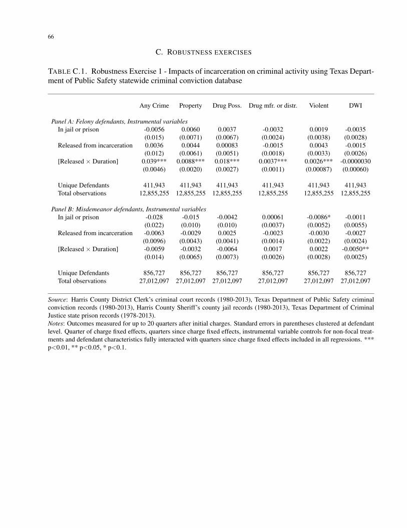
66
C. ROBUSTNESS EXERCISES
TABLE C.1. Robustness Exercise 1 - Impacts of incarceration on criminal activity using Texas Depart-ment of Public Safety statewide criminal conviction database
Any Crime Property Drug Poss. Drug mfr. or distr. Violent DWI
Panel A: Felony defendants, Instrumental variablesIn jail or prison -0.0056 0.0060 0.0037 -0.0032 0.0019 -0.0035
(0.015) (0.0071) (0.0067) (0.0024) (0.0038) (0.0028)Released from incarceration 0.0036 0.0044 0.00083 -0.0015 0.0043 -0.0015
(0.012) (0.0061) (0.0051) (0.0018) (0.0033) (0.0026)[Released × Duration] 0.039*** 0.0088*** 0.018*** 0.0037*** 0.0026*** -0.0000030
(0.0046) (0.0020) (0.0027) (0.0011) (0.00087) (0.00060)
Unique Defendants 411,943 411,943 411,943 411,943 411,943 411,943Total observations 12,855,255 12,855,255 12,855,255 12,855,255 12,855,255 12,855,255
Panel B: Misdemeanor defendants, Instrumental variablesIn jail or prison -0.028 -0.015 -0.0042 0.00061 -0.0086* -0.0011
(0.022) (0.010) (0.010) (0.0037) (0.0052) (0.0055)Released from incarceration -0.0063 -0.0029 0.0025 -0.0023 -0.0030 -0.0027
(0.0096) (0.0043) (0.0041) (0.0014) (0.0022) (0.0024)[Released × Duration] -0.0059 -0.0032 -0.0064 0.0017 0.0022 -0.0050**
(0.014) (0.0065) (0.0073) (0.0026) (0.0028) (0.0025)
Unique Defendants 856,727 856,727 856,727 856,727 856,727 856,727Total observations 27,012,097 27,012,097 27,012,097 27,012,097 27,012,097 27,012,097
Source: Harris County District Clerk’s criminal court records (1980-2013), Texas Department of Public Safety criminalconviction records (1980-2013), Harris County Sheriff’s county jail records (1980-2013), Texas Department of CriminalJustice state prison records (1978-2013).Notes: Outcomes measured for up to 20 quarters after initial charges. Standard errors in parentheses clustered at defendantlevel. Quarter of charge fixed effects, quarters since charge fixed effects, instrumental variable controls for non-focal treat-ments and defendant characteristics fully interacted with quarters since charge fixed effects included in all regressions. ***p<0.01, ** p<0.05, * p<0.1.
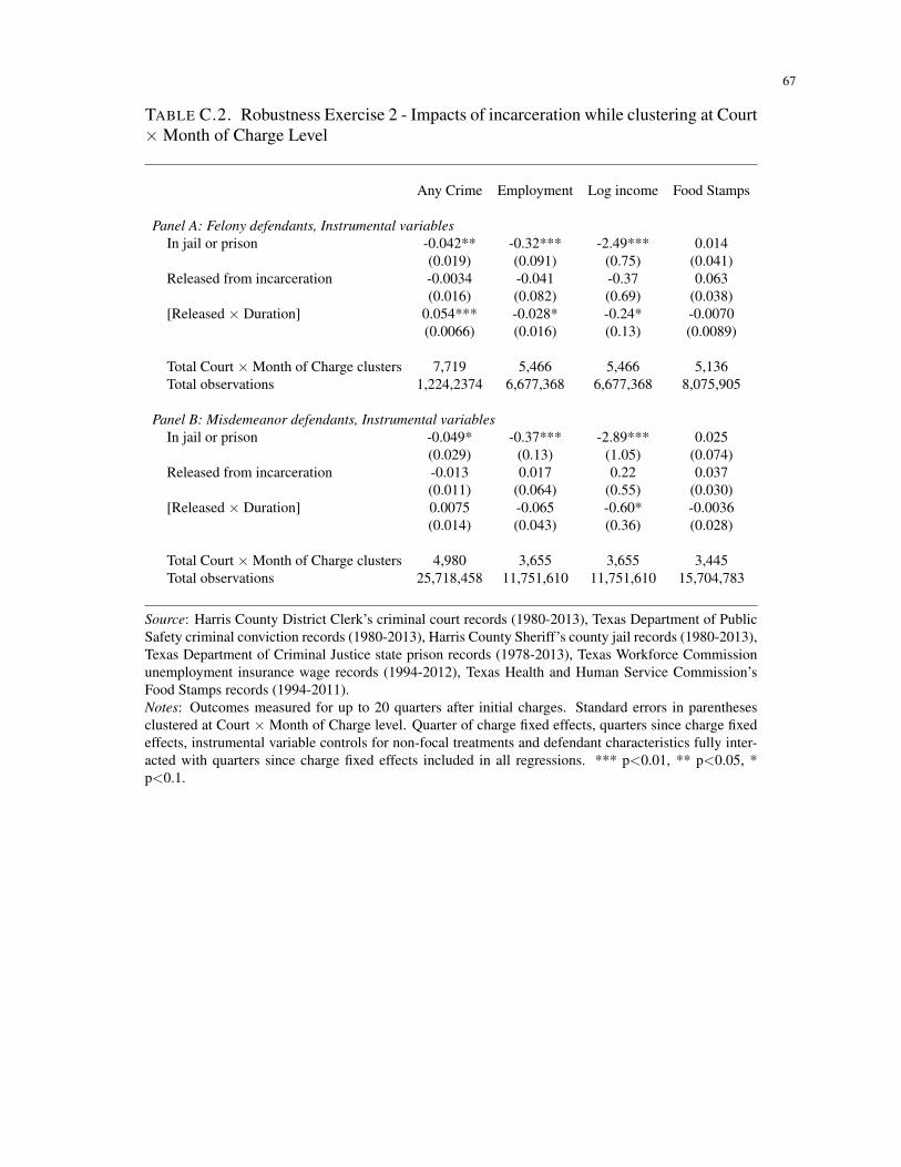
67
TABLE C.2. Robustness Exercise 2 - Impacts of incarceration while clustering at Court×Month of Charge Level
Any Crime Employment Log income Food Stamps
Panel A: Felony defendants, Instrumental variablesIn jail or prison -0.042** -0.32*** -2.49*** 0.014
(0.019) (0.091) (0.75) (0.041)Released from incarceration -0.0034 -0.041 -0.37 0.063
(0.016) (0.082) (0.69) (0.038)[Released × Duration] 0.054*** -0.028* -0.24* -0.0070
(0.0066) (0.016) (0.13) (0.0089)
Total Court ×Month of Charge clusters 7,719 5,466 5,466 5,136Total observations 1,224,2374 6,677,368 6,677,368 8,075,905
Panel B: Misdemeanor defendants, Instrumental variablesIn jail or prison -0.049* -0.37*** -2.89*** 0.025
(0.029) (0.13) (1.05) (0.074)Released from incarceration -0.013 0.017 0.22 0.037
(0.011) (0.064) (0.55) (0.030)[Released × Duration] 0.0075 -0.065 -0.60* -0.0036
(0.014) (0.043) (0.36) (0.028)
Total Court ×Month of Charge clusters 4,980 3,655 3,655 3,445Total observations 25,718,458 11,751,610 11,751,610 15,704,783
Source: Harris County District Clerk’s criminal court records (1980-2013), Texas Department of PublicSafety criminal conviction records (1980-2013), Harris County Sheriff’s county jail records (1980-2013),Texas Department of Criminal Justice state prison records (1978-2013), Texas Workforce Commissionunemployment insurance wage records (1994-2012), Texas Health and Human Service Commission’sFood Stamps records (1994-2011).Notes: Outcomes measured for up to 20 quarters after initial charges. Standard errors in parenthesesclustered at Court × Month of Charge level. Quarter of charge fixed effects, quarters since charge fixedeffects, instrumental variable controls for non-focal treatments and defendant characteristics fully inter-acted with quarters since charge fixed effects included in all regressions. *** p<0.01, ** p<0.05, *p<0.1.
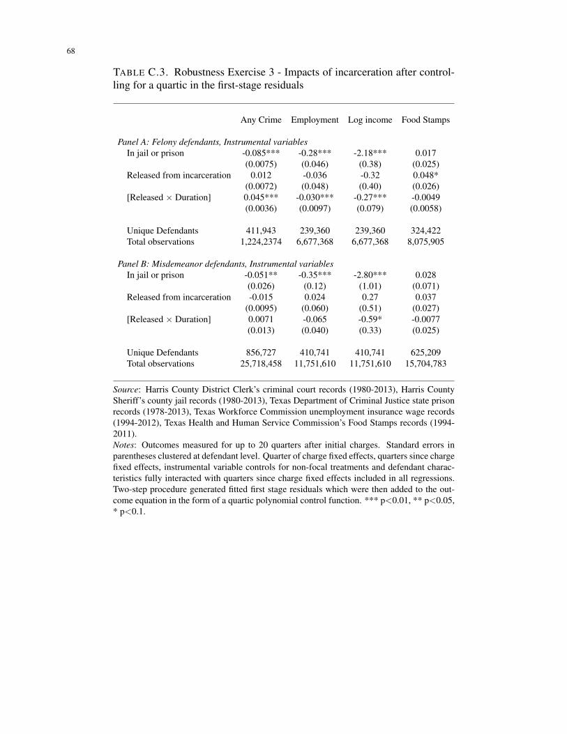
68
TABLE C.3. Robustness Exercise 3 - Impacts of incarceration after control-ling for a quartic in the first-stage residuals
Any Crime Employment Log income Food Stamps
Panel A: Felony defendants, Instrumental variablesIn jail or prison -0.085*** -0.28*** -2.18*** 0.017
(0.0075) (0.046) (0.38) (0.025)Released from incarceration 0.012 -0.036 -0.32 0.048*
(0.0072) (0.048) (0.40) (0.026)[Released × Duration] 0.045*** -0.030*** -0.27*** -0.0049
(0.0036) (0.0097) (0.079) (0.0058)
Unique Defendants 411,943 239,360 239,360 324,422Total observations 1,224,2374 6,677,368 6,677,368 8,075,905
Panel B: Misdemeanor defendants, Instrumental variablesIn jail or prison -0.051** -0.35*** -2.80*** 0.028
(0.026) (0.12) (1.01) (0.071)Released from incarceration -0.015 0.024 0.27 0.037
(0.0095) (0.060) (0.51) (0.027)[Released × Duration] 0.0071 -0.065 -0.59* -0.0077
(0.013) (0.040) (0.33) (0.025)
Unique Defendants 856,727 410,741 410,741 625,209Total observations 25,718,458 11,751,610 11,751,610 15,704,783
Source: Harris County District Clerk’s criminal court records (1980-2013), Harris CountySheriff’s county jail records (1980-2013), Texas Department of Criminal Justice state prisonrecords (1978-2013), Texas Workforce Commission unemployment insurance wage records(1994-2012), Texas Health and Human Service Commission’s Food Stamps records (1994-2011).Notes: Outcomes measured for up to 20 quarters after initial charges. Standard errors inparentheses clustered at defendant level. Quarter of charge fixed effects, quarters since chargefixed effects, instrumental variable controls for non-focal treatments and defendant charac-teristics fully interacted with quarters since charge fixed effects included in all regressions.Two-step procedure generated fitted first stage residuals which were then added to the out-come equation in the form of a quartic polynomial control function. *** p<0.01, ** p<0.05,* p<0.1.
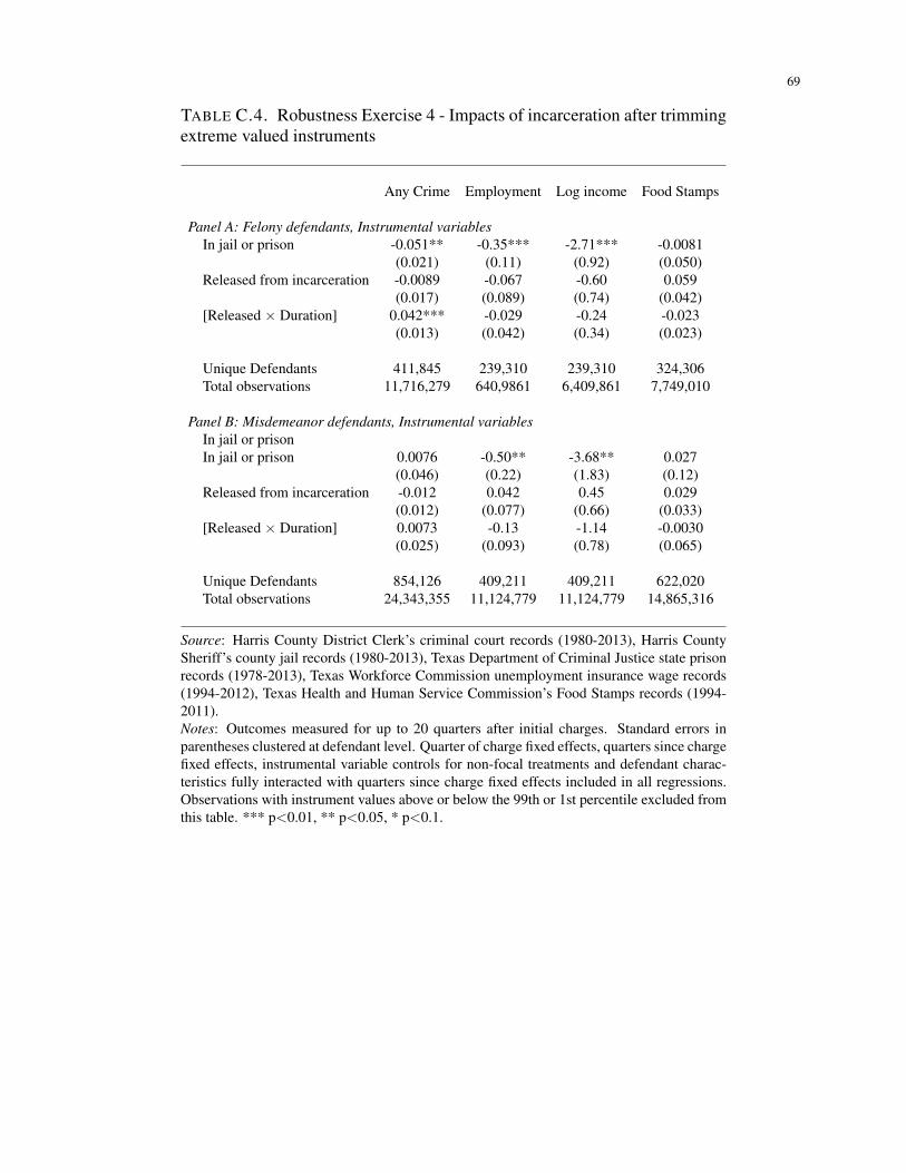
69
TABLE C.4. Robustness Exercise 4 - Impacts of incarceration after trimmingextreme valued instruments
Any Crime Employment Log income Food Stamps
Panel A: Felony defendants, Instrumental variablesIn jail or prison -0.051** -0.35*** -2.71*** -0.0081
(0.021) (0.11) (0.92) (0.050)Released from incarceration -0.0089 -0.067 -0.60 0.059
(0.017) (0.089) (0.74) (0.042)[Released × Duration] 0.042*** -0.029 -0.24 -0.023
(0.013) (0.042) (0.34) (0.023)
Unique Defendants 411,845 239,310 239,310 324,306Total observations 11,716,279 640,9861 6,409,861 7,749,010
Panel B: Misdemeanor defendants, Instrumental variablesIn jail or prisonIn jail or prison 0.0076 -0.50** -3.68** 0.027
(0.046) (0.22) (1.83) (0.12)Released from incarceration -0.012 0.042 0.45 0.029
(0.012) (0.077) (0.66) (0.033)[Released × Duration] 0.0073 -0.13 -1.14 -0.0030
(0.025) (0.093) (0.78) (0.065)
Unique Defendants 854,126 409,211 409,211 622,020Total observations 24,343,355 11,124,779 11,124,779 14,865,316
Source: Harris County District Clerk’s criminal court records (1980-2013), Harris CountySheriff’s county jail records (1980-2013), Texas Department of Criminal Justice state prisonrecords (1978-2013), Texas Workforce Commission unemployment insurance wage records(1994-2012), Texas Health and Human Service Commission’s Food Stamps records (1994-2011).Notes: Outcomes measured for up to 20 quarters after initial charges. Standard errors inparentheses clustered at defendant level. Quarter of charge fixed effects, quarters since chargefixed effects, instrumental variable controls for non-focal treatments and defendant charac-teristics fully interacted with quarters since charge fixed effects included in all regressions.Observations with instrument values above or below the 99th or 1st percentile excluded fromthis table. *** p<0.01, ** p<0.05, * p<0.1.
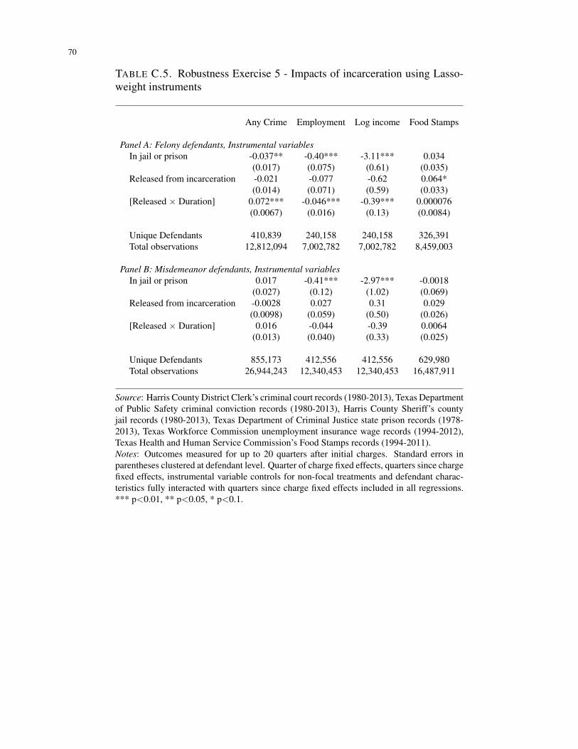
70
TABLE C.5. Robustness Exercise 5 - Impacts of incarceration using Lasso-weight instruments
Any Crime Employment Log income Food Stamps
Panel A: Felony defendants, Instrumental variablesIn jail or prison -0.037** -0.40*** -3.11*** 0.034
(0.017) (0.075) (0.61) (0.035)Released from incarceration -0.021 -0.077 -0.62 0.064*
(0.014) (0.071) (0.59) (0.033)[Released × Duration] 0.072*** -0.046*** -0.39*** 0.000076
(0.0067) (0.016) (0.13) (0.0084)
Unique Defendants 410,839 240,158 240,158 326,391Total observations 12,812,094 7,002,782 7,002,782 8,459,003
Panel B: Misdemeanor defendants, Instrumental variablesIn jail or prison 0.017 -0.41*** -2.97*** -0.0018
(0.027) (0.12) (1.02) (0.069)Released from incarceration -0.0028 0.027 0.31 0.029
(0.0098) (0.059) (0.50) (0.026)[Released × Duration] 0.016 -0.044 -0.39 0.0064
(0.013) (0.040) (0.33) (0.025)
Unique Defendants 855,173 412,556 412,556 629,980Total observations 26,944,243 12,340,453 12,340,453 16,487,911
Source: Harris County District Clerk’s criminal court records (1980-2013), Texas Departmentof Public Safety criminal conviction records (1980-2013), Harris County Sheriff’s countyjail records (1980-2013), Texas Department of Criminal Justice state prison records (1978-2013), Texas Workforce Commission unemployment insurance wage records (1994-2012),Texas Health and Human Service Commission’s Food Stamps records (1994-2011).Notes: Outcomes measured for up to 20 quarters after initial charges. Standard errors inparentheses clustered at defendant level. Quarter of charge fixed effects, quarters since chargefixed effects, instrumental variable controls for non-focal treatments and defendant charac-teristics fully interacted with quarters since charge fixed effects included in all regressions.*** p<0.01, ** p<0.05, * p<0.1.
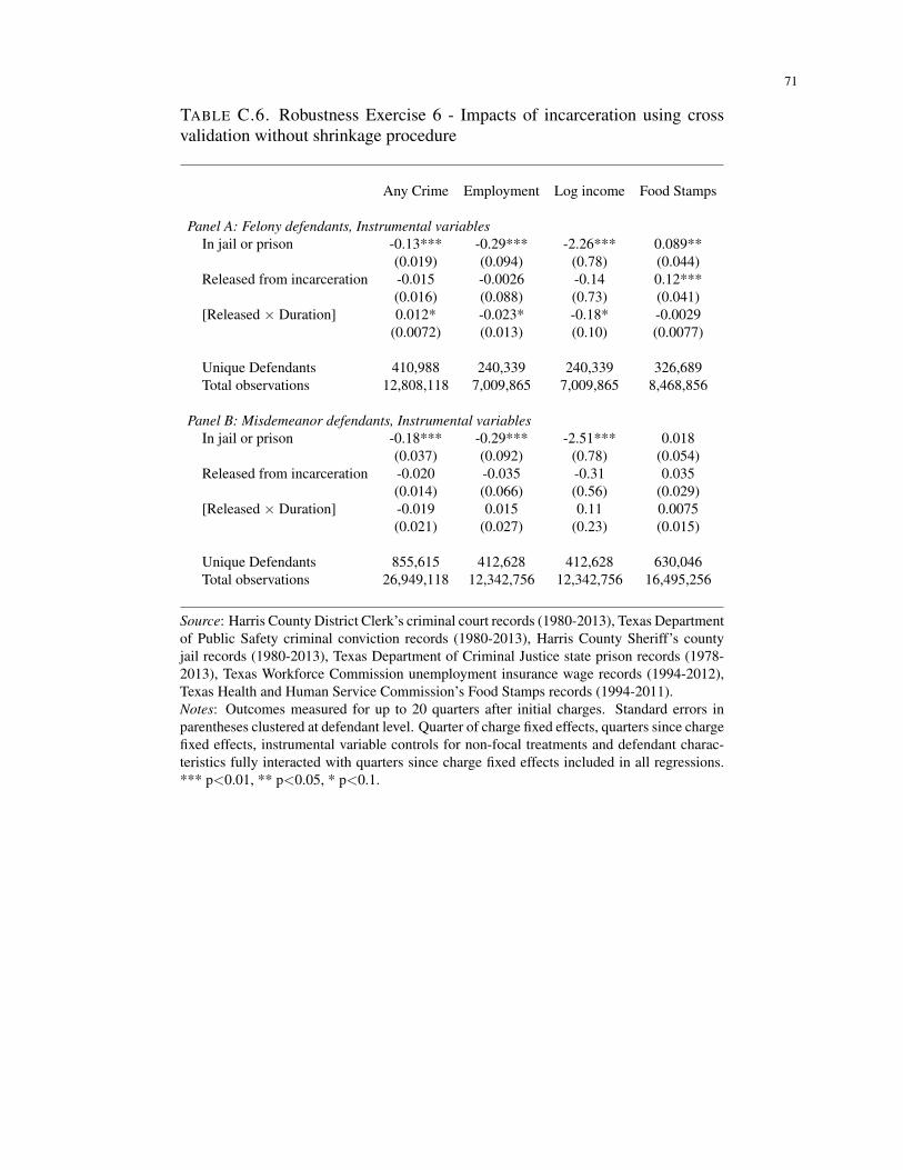
71
TABLE C.6. Robustness Exercise 6 - Impacts of incarceration using crossvalidation without shrinkage procedure
Any Crime Employment Log income Food Stamps
Panel A: Felony defendants, Instrumental variablesIn jail or prison -0.13*** -0.29*** -2.26*** 0.089**
(0.019) (0.094) (0.78) (0.044)Released from incarceration -0.015 -0.0026 -0.14 0.12***
(0.016) (0.088) (0.73) (0.041)[Released × Duration] 0.012* -0.023* -0.18* -0.0029
(0.0072) (0.013) (0.10) (0.0077)
Unique Defendants 410,988 240,339 240,339 326,689Total observations 12,808,118 7,009,865 7,009,865 8,468,856
Panel B: Misdemeanor defendants, Instrumental variablesIn jail or prison -0.18*** -0.29*** -2.51*** 0.018
(0.037) (0.092) (0.78) (0.054)Released from incarceration -0.020 -0.035 -0.31 0.035
(0.014) (0.066) (0.56) (0.029)[Released × Duration] -0.019 0.015 0.11 0.0075
(0.021) (0.027) (0.23) (0.015)
Unique Defendants 855,615 412,628 412,628 630,046Total observations 26,949,118 12,342,756 12,342,756 16,495,256
Source: Harris County District Clerk’s criminal court records (1980-2013), Texas Departmentof Public Safety criminal conviction records (1980-2013), Harris County Sheriff’s countyjail records (1980-2013), Texas Department of Criminal Justice state prison records (1978-2013), Texas Workforce Commission unemployment insurance wage records (1994-2012),Texas Health and Human Service Commission’s Food Stamps records (1994-2011).Notes: Outcomes measured for up to 20 quarters after initial charges. Standard errors inparentheses clustered at defendant level. Quarter of charge fixed effects, quarters since chargefixed effects, instrumental variable controls for non-focal treatments and defendant charac-teristics fully interacted with quarters since charge fixed effects included in all regressions.*** p<0.01, ** p<0.05, * p<0.1.
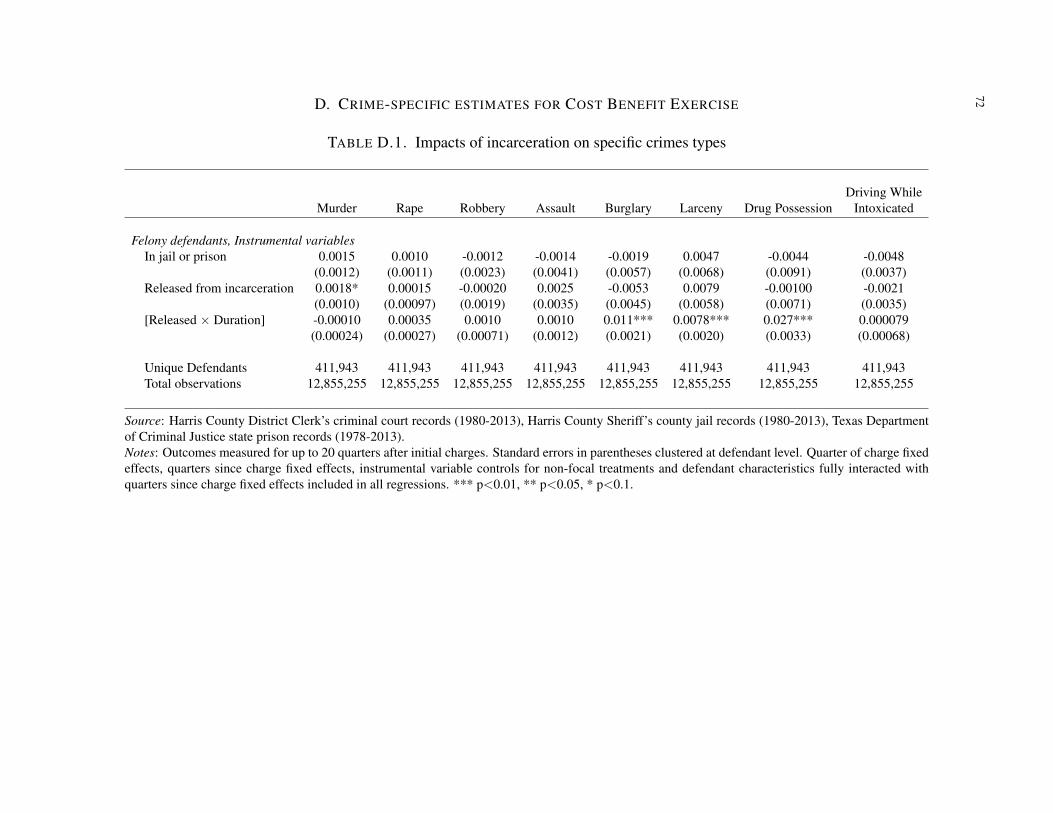
72D. CRIME-SPECIFIC ESTIMATES FOR COST BENEFIT EXERCISE
TABLE D.1. Impacts of incarceration on specific crimes types
Driving WhileMurder Rape Robbery Assault Burglary Larceny Drug Possession Intoxicated
Felony defendants, Instrumental variablesIn jail or prison 0.0015 0.0010 -0.0012 -0.0014 -0.0019 0.0047 -0.0044 -0.0048
(0.0012) (0.0011) (0.0023) (0.0041) (0.0057) (0.0068) (0.0091) (0.0037)Released from incarceration 0.0018* 0.00015 -0.00020 0.0025 -0.0053 0.0079 -0.00100 -0.0021
(0.0010) (0.00097) (0.0019) (0.0035) (0.0045) (0.0058) (0.0071) (0.0035)[Released × Duration] -0.00010 0.00035 0.0010 0.0010 0.011*** 0.0078*** 0.027*** 0.000079
(0.00024) (0.00027) (0.00071) (0.0012) (0.0021) (0.0020) (0.0033) (0.00068)
Unique Defendants 411,943 411,943 411,943 411,943 411,943 411,943 411,943 411,943Total observations 12,855,255 12,855,255 12,855,255 12,855,255 12,855,255 12,855,255 12,855,255 12,855,255
Source: Harris County District Clerk’s criminal court records (1980-2013), Harris County Sheriff’s county jail records (1980-2013), Texas Departmentof Criminal Justice state prison records (1978-2013).Notes: Outcomes measured for up to 20 quarters after initial charges. Standard errors in parentheses clustered at defendant level. Quarter of charge fixedeffects, quarters since charge fixed effects, instrumental variable controls for non-focal treatments and defendant characteristics fully interacted withquarters since charge fixed effects included in all regressions. *** p<0.01, ** p<0.05, * p<0.1.