Embed Size (px)
Citation preview

0
The Crime Reducing Effect of Education
Stephen Machin*, Olivier Marie**, and Sun ica Vuji ***
September 2010 - Revised
* Department of Economics, University College London and Centre for EconomicPerformance, London School of Economics
** Research Centre for Education and the Labour Market (ROA), MaastrichtUniversity and Centre for Economic Performance, London School of Economics
*** Department of Management, London School of Economics
AbstractIn this paper, we study the crime reducing potential of education, presenting causalstatistical estimates based upon a law that changed the compulsory school leaving age inEngland and Wales. We frame the analysis in a regression-discontinuity setting anduncover significant decreases in property crime from reductions in the proportion ofpeople with no educational qualifications and increases in the age of leaving school thatresulted from the change in the law. The findings show that improving education canyield significant social benefits and can be a key policy tool in the drive to reduce crime.
JEL Keywords: Crime; Education; School Leaving Age.JEL Classifications: I2; K42.
AcknowledgementsThis is a heavily revised version of Machin, Marie and Vuji (2010). Machin and Vujiwish to thank the Economic and Social Research Council for funding under researchgrant RES-000-22-0568. Marie would like to thank the Executive Research Agency ofthe European Union for funding under the Marie Curie IEF grant number 252572. Usefulcomments were received from Brian Bell, Lance Lochner, two referees and participantsin numerous seminars and conferences.

1
1. Introduction
Crime reduction is high on the public policy agenda, not least because of the large
economic and social benefits it brings. Indeed, research on the determinants of crime
points in several directions as to how crime reduction can be facilitated. A relatively large
body of research undertaken by social scientists considers the potential for expenditures
on crime fighting resources (like increased police presence, or new crime fighting
technologies), or on particular policies to combat crime.1 Other work focuses more on the
characteristics of criminals and considers which characteristics are more connected to
higher criminal participation. In this latter case, policies that affect these characteristics
can, if implemented successfully, be used to counter crime.
In this paper, we focus on one such characteristic that has received some attention
in the quantitative social science literature on the determinants of crime, namely
education. In this literature, there is a (relatively small) body of work that attempts to
establish a causal connection between crime and education (most notably the seminal
paper of Lochner and Moretti, 2004) and a vast literature from various social science
disciplines that does not.2 A drawback associated with almost all of this latter work is that
it is difficult to ascertain whether the direction of causation flows from education to crime
(and not the other way around). This, of course, matters if one wishes to consider
appropriate policy responses to empirical findings.
1 UK evidence on the crime-police relation (in the context of the July 2005 terror attacks that hit London)is presented in Draca, Machin and Witt (2010) and evidence of crime reduction from a specific policy (theStreet Crime Initiative) appears in Machin and Marie (2010).2 Examples from the criminology literature include Farrington (1986, 2001) and from the educationliterature include Sabates (2008, 2009) and Sabates and Feinstein (2008). There is much less work byeconomists. See Lochner (2010) for a broader overview of the crime and education literature.

2
Our focus is on empirically analysing the crime reducing potential of education
and we present causal statistical evidence based upon a law that changed the compulsory
school leaving age in England and Wales. As the raising of the school leaving age
generated sharp increases in education for those affected, we frame our analysis in a
regression-discontinuity setting looking at birth cohorts just before and after the law
change. We show that there were significant property crime reductions associated with
the extra education people obtained (or were forced to obtain) from the raising of the
school leaving age. The implications of these findings are clear. Not only do they show
that improving the education levels and attainment of individuals who would otherwise
be on the margins of crime participation can act as a key policy tool in the drive to reduce
crime, but also that such educational improvements can yield sizable social benefits.
The rest of the paper is organised as follows. Section 2 offers a brief discussion of
the theoretical background on the relationship between education and crime, describes the
data sources used, shows some descriptive evidence on the association between crime
and education and discusses the school leaving age reform we consider. Section 3
describes the empirical strategies we implement and presents the results, together with a
calculation of the social benefits that follow from the estimated crime reducing effect of
education. Concluding remarks are given in the last section of the paper.
2. Crime Reducing Education Mechanisms, Data and Descriptive Analysis
Mechanisms Where Education Changes Can Impact on Crime
There are number of theoretical reasons why education may have an effect on
crime. From the existing socio-economic literature there are (at least) three main channels

3
through which schooling might affect criminal participation: income effects, time
availability, and patience or risk aversion. For most crimes, one would expect that these
factors induce a negative effect of schooling on crime, although ultimately this is an
empirical question. We briefly consider each of the three mechanisms in turn:
i) The income effect works through education increasing the returns to legitimate work
and/or raising the opportunity costs of illegal behaviour (Lochner, 2004; Lochner and
Moretti, 2004; Hjalmarsson, 2008). Empirical evidence supports the notion: for example,
Grogger (1998) links crime to wages, concluding that youth offending behaviour is
responsive to price incentives and that falling real wages may have been an important
factor in rising youth crime during the 1970s and 1980s. Machin and Meghir (2004) look
at cross-area changes in crime and the low wage labour market in England and Wales.
They find that crime fell in areas where wage growth in the bottom 25th percentile of the
distribution was faster and conclude that “improvements in human capital accumulation
through the education system or other means… enhancing individual labour market
productivity… would be important ingredients in reducing crime.”
Conversely, there is also some evidence that education can also increase the
earnings from crime as certain skills acquired in school may be inappropriately used for
criminal activities. Levitt and Lochner (2001) find that males with higher scores on
mechanical information tests had increased offence rates. Lochner (2004) also estimates
that across cohorts, increases in average education are associated with 11% increase in
white-collar arrest rates (although this estimated effect is not statistically significant).
ii) Time spent in education may also be important for teenagers in terms of limiting the
time available for participating in criminal activity. This ‘self-incapacitation’ effect was

4
documented by Tauchen et al. (1994) who found that time spent at school (and work)
during a year is negatively correlated to the probability of arrest that year. Hjalmarsson
(2008) looked at the opposite relationship, studying the impact of being arrested and
incarcerated before finishing school on probability of graduating high school. Her results
suggest that the more times you are caught committing crime and the amount of time
spent in prison both greatly increase the likelihood of becoming a high school dropout.
As these still may be endogenous decisions, Jacob and Lefgren (2003) instrument
days off school with exogenous teacher training days and Luallen (2006) uses unexpected
school closings driven by teacher strikes as an instrument for student absence from
school. Both papers find important incapacitation effects of education on criminal
participation. However, they also report that violent offences increase while school is in
session, a finding that is attributed to a concentration effect.3 Anderson (2009) also
reports US evidence, based on minimum high school dropout ages that vary across states,
in line with the notion that keeping youth in school decreases arrest rates.
iii) Education may also influence crime through its effect on patience and risk aversion
(Lochner and Moretti, 2004). Here, future returns from any activity are discounted
according to one’s patience in waiting for them. Thus, individuals with a lot of patience
have low discount rates and value future earnings more highly as compared to those with
high discount rates. Oreopoulos (2007) summarizes a sample of studies from the
psychological and neurological literature, concluding that young people who drop out of
school tend to be myopic and more focussed on immediate costs from schooling (stress
from taking tests, uninteresting curricula, foregone earnings, etc.), rather than on future
3 This is the geographical proximity of a large number of youths – in the educational establishment – whichmay result in increasing the probability of violent encounters.

5
gains from an additional year of schooling. This line of literature also suggests that
adolescents lack abstract reasoning skills and are more predisposed to risky behaviour.
Education can increase patience, which reduces the discount rate of future earnings and
hence reduces the propensity to commit crimes. Education may also increase risk
aversion that, in turn, increases the weight given by individuals to a possible punishment
and consequently reduces the likelihood of committing crimes.
Data Description
There are a number of pertinent data issues that we next need to discuss, as they
are relevant in the context we study. First, there is the issue that crime measurement is
different across data sources. Second, whilst some micro-data on crime does contain
information on the characteristics of criminals, the majority does not. In the latter case,
we need some means of matching crime data to education data.
Probably the most commonly used source of crime data in quantitative research is
information on criminal offences recorded by the police. As not all of these are solved or
cleared up, this type of data does not contain information on characteristics of the
individuals committing these recorded offences. Unless these data are aggregated to some
geographical level (like police force area) and matched to education data at this level,
then it is not possible to use these data to study the empirical relationship between crime
and education. Being realistic, such spatial aggregation does not offer much hope to
credibly study the research question of interest in this paper.
The other main form of crime data available comes from those individuals who
enter the criminal justice system after having been apprehended and charged for a crime.
In England and Wales, the Offenders Index Database (OID) contains criminal history

6
data for offenders convicted of standard list offences from 1963 onwards.4 The data
(which are described in detail in Data Appendix A) are derived from the court
appearances system and are updated quarterly. The Index was created purely for research
and statistical analysis. Its main purpose is to provide full criminal history data on a
randomly selected sample of offenders.
We have access to OID data on anonymous samples for offenders sentenced
during four weeks each year. We also have the entire pre- and post-court appearance
history of these individuals. However, there is no information on a defendant’s education
level in the OID and so the data needs to be aggregated to connect to education data from
other sources. A big advantage (certainly relative to recorded offences data) is that some
demographic characteristics are available in the OID, notably age and gender.
We therefore calculated offending rates (per 1000 population) using Office for
National Statistics (ONS) population data by age cohort and year, separately for men and
women. In doing so, criminal offences were also broadly categorised as property crimes
(burglary and theft and handling stolen goods) and violent crimes (violence against the
person and robbery). These offending rates can be matched to education data from other
micro-data sources where education measures can be collapsed into age by year (by
gender) cells.
We investigated several possible sources of data containing individual education
characteristics to match to the OID. The three main candidates were: the Family
Expenditure Survey (FES); the General Household Survey (GHS); and the Labour Force
Survey (LFS). The best match turned out to be the GHS for several reasons. First, it
4 Standard list offences are all indictable or triable offences, plus a few of the more serious summaryoffences.

7
enables us to go further back in time, with a start year of 1972 with well defined
education data, as compared to 1978 in the FES and 1979 (with some missing years as
the original survey was only bi-annual) in the LFS. Starting earlier in the 1970s is
important, to ensure we have data on young enough people before and after when the
education reform we consider occurred. Second, we can consider two measures of
education - age left school and whether individuals have no educational qualifications - in
the GHS, whereas the FES only has information on age left full-time education and the
LFS contains information on no qualifications (though not consistently in all years) and
age left full-time education. Thirdly, as we are planning to look at the causal impact via a
school leaving age law, the GHS has the more appropriate age left school measure
whereas the other two data sources relate to school and non-school terminal age. Data
Appendix A describes more fully how we matched the OID and GHS data for the main
analysis in this paper. Our sample consists of people aged 18-40 born between 1946 and
1970 from OID and GHS data across the 1972 to 1996 time period.
Other data sources with information on crime activity do permit non-causal
analyses to be undertaken. For example, Census micro-data in a number of countries does
contain information on both incarceration (individuals who are in prison service
establishments) and on individual education levels.5 However, in the UK context, only
the 2001 Census has good enough data on individual education and so only permits a
cross-sectional analysis. The British Crime Survey (BCS) also contains information on
the respondent’s education level and rudimentary self-reported information on criminal
histories.
5 Indeed, a large part of the US paper by Lochner and Moretti (2004) uses US Census data. Their majoradvantage is having several US Censuses when both imprisonment and education data were simultaneouslyavailable.

8
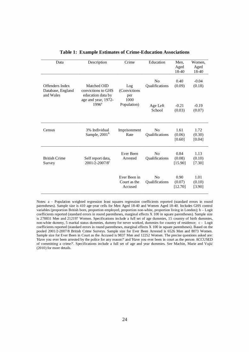
For purposes of illustration, Table 1 uses these different data sources to show
some non-causal regression estimates of the association between crime and education for
18-40 year-old men and women. Like other studies in the large literature in this area, they
show a significant empirical negative correlation between crime and age left education
and a positive association with no qualifications. This is true for the matched OID-GHS
data in the upper panel (except for the no qualifications association for women), the 2001
Census data on imprisonment and no qualifications in the middle panel and the 2001/2-
2007/8 British Crime Survey self-report data on ever being arrested or ever being in court
as the defendant.
Of course, these are simply correlations and are not easy to interpret as there are
many other confounding factors at play. For the cases of the cohort models, consider a
simple least squares regression of a measure of offending for a particular age cohort a in
year t ( atO ) with an education variable ( atE ) as an explanatory variable and jatX (
,J,,j L21= ) being a set of other control variables:
at
J
jjatjatat uXEO +++= ∑
=010 λαα
(1)
where atu is an error term.
If unobserved characteristics of cohorts drive crime participation, but also
education, then least squares estimates of 1α (like those given in Table 1) will be biased.
This is a key issue to the extent that unobserved characteristics affecting schooling
decisions may be correlated with unobservables influencing the decision to engage in
crime. For example, 1α could be estimated to be negative, even if schooling has no
causal effect on crime. This would be the case if individuals who have high criminal
returns were likely to spend most of their time committing crime rather than work,

9
regardless of their educational background. As long as education does not increase the
returns to crime, these individuals are likely to drop out of further education. As a result,
we might observe a negative correlation between education and crime even though there
is no causal effect between the two. To implement a causal approach that is plausible
requires an instrument for education, which is the issue we turn to next.
The School Leaving Age Reform
Identification of a causal education impact on crime is generated from a
compulsory school leaving increase that affected 15 year-olds in England and Wales in
the early 1970s. Like Lochner and Moretti’s (2004) approach, which exploits changes in
school leaving age laws across US states, we use the raising of the school leaving from
age 15 to 16 that took force in England and Wales in September 1972 (thus affecting the
cohort of children finishing school in 1973) as an instrumental variable in our empirical
analysis.6
The raising of the school leaving age generates a discontinuity in education
measures at the time when the reform was implemented. In the next section of the paper
we will show results from empirical analysis of relationships between the law change and
crime and education using instrumental variable and regression discontinuity methods.
However, before moving on to this, we first illustrate discontinuities induced by the
reform. Figure 1 uses GHS data to show the average age left school and the proportion
6 There was an earlier increase in the compulsory school leaving age from 14 to 15 that took force in April1947. This and (less frequently) the law we focus on here have been considered in a growing literature inlabour and health economics. Harmon and Walker (1995) and Oreopoulos (2006) focus on the causalimpact of education on earnings (see also Devereux and Hart's (2010) robust criticism of the Oreopoulospaper). Galindo-Rueda (2003), Chevalier (2004), and Chevalier et al. (2005) look at the effect of parentalincome on education of their children. Oreopoulos (2006), Doyle et al. (2007), and Lindeboom et al. (2009)examine the impact of education on health. We are the first to consider the school leaving age reforms inEngland and Wales to study the causal impact of education on crime. Of course, we do not have data oncrime for young enough people before and after the 1947 increase and so can only consider the 1972 law.

10
with no educational qualifications for men aged 18-40 who were born between 1950 and
1965. The vertical line in Figure 1 shows the timing of the law change. There is a very
clear and marked fall in the proportion with no educational qualifications in the upper
Figure and a sharp increase in the average school leaving age in the lower Figure.
Evidently there was a big discontinuity in educational outcomes induced by the law
change. The non-overlapping nature of the confidence intervals before and after the
discontinuity in the Figure shows that the changes were clearly statistically significant.
Figure 2 also shows a marked fall in the OID conviction rate for men leaving school after
the school leaving reform. There is a very clear and distinct drop in the conviction rate at
the discontinuity, after which convictions trend upwards. The existence of clear and
significant discontinuities in both crime and education is highly suggestive of a causal
impact, the issue and detail of which we next empirically explore.
3. Causal Estimates of the Crime-Education Relation
In this section of the paper, we present instrumental variable (IV) and regression-
discontinuity (RD) based estimates of the relationship between crime and education. We
begin with the IV estimates, move next to the RD estimates, show a series of robustness
tests and last present some calculations of the social benefits of crime reduction induced
by improved education.
Instrumental Variable Estimates
Identification of the causal effect of education on crime is achieved through
inclusion in a first stage education regression of a dummy variable that records the
exogenous change in the minimum school leaving age that occurred in England and

11
Wales, as described above. We define a dummy variable (SLA) equal to one for
individuals who entered their last compulsory school year in 1972 and later. The
discontinuity is generated for the 1972 cohort who were the first to face a minimum
school leaving age of 16 (SLA) when they left school in 1973.7
The relevant crime and education reduced forms are
at
J
jjatjatat vXSLAO +++= ∑
=010 φββ
(2)
at
J
jjatjatat XSLAE υϕδδ +++= ∑
=010
The crime structural form therefore used to yield causal estimates is
at
J
jjatjatat XEO εσθθ +++= ∑
=010 (3)
where the IV estimate of the coefficient on the education variable in (3) is the ratio of the
reduced form coefficients in (2), 111 /δβθ = .
In this framework, it is important whether the change in compulsory schooling
age legislation acts as a valid instrument. A legitimate instrument for education in
equation (3) is a variable that: (i) significantly explains part of the variation in education;
and (ii) is not correlated with the unobservables that are correlated with both offending
and education. Put alternatively, it is a variable that is a determinant of schooling that can
legitimately be omitted from equation (1). Our estimates hinge on the notion that SLA
fulfils these requirements. The first issue is a statistical one which, as shown below, is
satisfied as SLA is a strong predictor of education. Regarding the second issue, changes
in compulsory attendance laws have not historically been concerned by problems with
7 In most years of the GHS we do not know month of birth. Therefore, in a similar way to Devereux andHart (2010) in their analysis of the 1947 reform which was introduced in April 1947, where they code theirreform variable equal to 0 for pre-1933 birth cohorts, to 0.75 for the 1933 cohort and 1 to the post-1933cohorts, we code SLA to 0.33 for the 1957 birth cohort (since the reform began on 1 September 1972).

12
crime. To our knowledge, legislators enacting the laws did not act in response to concerns
with juvenile delinquency, youth unemployment, or other factors related to crime, thus
making schooling laws an appropriate instrument.
It also needs to be acknowledged that the variation induced by the instrument is
local in nature, as it has an impact at the bottom of the education distribution and not at
the top. This is because people near the top would have stayed on after the compulsory
school leaving age anyway and the change would not affect them. Therefore, the effect
that our empirical approach estimates is the local average treatment (LATE) effect among
those who alter their treatment status because they react to the instrument. For this
reason, we consider effects separately for the continuous age left school measure, but also
more appropriately for the no qualifications variable.
Baseline Estimates
The first set of baseline estimates for total conviction rates are given in Table 2.
The Table shows four sets of estimates of the reduced and structural form crime and
education models described in equations (2) and (3). Columns (1)-(5) respectively show
the crime reduced form, education reduced form and crime structural form for the no
qualifications and age left school variables from the GHS-OID 1972-96 cohort year data
for men aged 18-40 who were born between 1946-70. Columns (6)-(10) do the same, but
for a sample of +/– four birth cohorts around the discontinuity point.
Both crime and education reduced forms show a strong and significant effect of
the school leaving age increase. In column (1) there is a 4.7 percent point fall in the
conviction rate in the years after the education reform, revealing a statistically significant
crime reduced form. In columns (2) and (5), the same is true of education, with a 5.7

13
percent fall in the proportion with no qualifications and an increase of almost a quarter of
a year (0.22) in the average school leaving age.
These significant crime and education effects combine into a significant causal
impact of education on crime. Column (3) shows the IV estimate for the no qualifications
variable. It is positive and strongly significant at 0.82. Interestingly this is larger than the
comparable non-causal, least squares estimate of 0.40 reported in the upper panel of
Table 1. A strong crime reduction from education is also seen in the age left school
specification in column (5) where a 10 percent increase in age left school lowers crime by
2.1 percent.8 In this case, this is exactly the same as the least squares estimate in Table 1.
The fact that the IV estimates lie at or above comparable least squares estimates
draws an interesting parallel with the literature on the causal effect of education on
earnings where the same pattern seems to occur (see Card, 1999). It does not seem
unreasonable to think that the same kind of mechanisms discussed in that literature,
highlighting the fact that the IV estimates pick up a local average treatment effect on low
education individuals, also apply in interpreting the crime-education results reported here.
Discontinuity Sample
As Figures 1 and 2 show, there are sharp crime and education discontinuities for
cohorts affected by the school leaving age law. It therefore is natural to focus more on
observations nearer to the discontinuity point. The specifications in columns (6) to (10)
of Table 2 show results from focussing in on a window defined as +/– four years around
8 Table B1 in Appendix B shows results for women. The education reduced forms are, if anything, strongerfor women, but the crime reduced forms are imprecisely determined and therefore so is the IV estimate.This imprecision in estimates is not surprising given the very low female offending rates, especiallyamongst the older women in our age 18-40 cohorts, seen in the data.

14
the treated birth cohort at the discontinuity (i.e. those individuals born between 1953 and
1961).
The main substantive change, which is probably not surprising given the
narrowing of the cohort window, is that the estimated reduced form coefficients rise in
absolute magnitude. This is the case in both the crime and education reduced forms such
that the IV estimates remain similar. For the no qualifications and age left school
specifications the IV estimate is strongly significant, identifying a causal crime reducing
effect of education.
Inverse Distance Weighting
The second way we hone in more on the discontinuity is to note that the policy
treatment induced by the law change is binding for the cohort right near the discontinuity
in September 1957. We have thus also generated inverse distance weighted estimates
where we place more weight on those observations nearer to the discontinuity point and
less as they are further away.9 We do this to ensure that identification predominantly
comes from variation close to the discontinuity, weighting by 1/d where d is distance in
birth years from the discontinuity.
The inverse distance weighted (IDW) results are given in Table 3, which is of the
same form as Table 2. The pattern of results is qualitatively the same as in Table 2
although the coefficient on the school leaving age dummy variable tends to increase in
magnitude (in absolute terms) in the full sample and in the discontinuity sample. The
IDW IV coefficient estimates of 0.88 in the no qualifications specification and of –0.27 in
9 A similar approach of inverse distance weighting is adopted in a very different context by Gibbons,Machin and Silva (2009) in their analysis of housing valuations of school quality where discontinuitiesarise as children rarely cross administrative boundaries to attend school.

15
the age left school specification show a strong and significant causal impact of education
on crime.10
Estimates by Broad Crime Type
Table 4 shows separate estimates from models of property crime and violent
crime for the discontinuity sample. There are two panels in the Table, the upper panel
focussing on the population weighted models and the lower panel reporting IDW
estimates. There is evidence of a strong and significant crime reducing education effect
for property crime, but the violent crime specifications are much less precisely
determined and the estimated effects are insignificantly different from zero. In the case
of property crimes, the IV estimates suggest that a one percent point fall in the proportion
with no educational qualifications reduces crime by between 0.85 and 1.00 percent. A 1
percent increase in the average age men leave school generates a 0.25 to 0.30 percent fall
in their probability of being convicted for a property crime.
Robustness
In Table 5 we present a number of robustness checks of our main discontinuity
sample results for property crimes. The upper panel of the Table considers robustness to
functional form, for results from the standard regression models and for the inverse
distance weighted specifications. Four such robustness checks are reported, revealing
how the estimates change on adding birth cohort age specific trends, linear and quadratic
birth cohort variables or linear splines on each side of the discontinuity. In all cases the
10 The specifications in Tables 2 and 3 include full sets of age and year dummies. This choice of functionalform is driven by the data matching procedure (see Data Appendix A). Adopting a different specificationfocussing more on birth cohort, for example as done by including a quartic in birth cohort and age (or agedummies) in the earnings-education studies of Oreopoulos (2006) or Devereux and Hart (2010), producedsimilar results which, if anything, were slightly larger in magnitude. For this latter choice of functionalform in the IDW models, the estimated IV coefficients (standard error) were 0.777 (0.316) and -0.249(0.092) respectively in the no qualifications and age left school specifications. Other functional formrobustness checks are reported below in Table 5.

16
IV estimates remain statistically significant and of similar magnitude to the baseline
estimates in Table 4. If anything, the magnitude of the causal estimates increase after
these amendments of functional form.
In the lower panel of Table 5 we also report the results from a simple falsification
exercise which sets a ‘placebo’ school leaving age law in September 1969. The first
cohort affected would have been the 1954 one and we include all males aged 18 to 40
born between 1947 and 1957 (to exclude those affected by the actual school leaving age
increase). We find all the IV estimates to be extremely small in magnitude and none are
even close to being significant. These robustness checks validate the causal nature of the
causal relationship observed despite the potential issues of the rising trends in crime and
education over the years.
Discussion and Social Benefits Calculation
The empirical analysis identifies a robust, causal impact of education on property
crime. Results on violent crime are more volatile and no clear pattern emerged, possibly
because of the noisier nature of the data, or perhaps (in line with the arguments discussed
in the context of existing literature in Section 2) because the crime reducing potential of
education applies more to property than violent crimes. However, the vast majority of
crimes that occur are property crimes (these represent more than 70 percent of offences
recorded by the police and indictable offences tried in courts). Given that we have
identified a sizable crime reducing impact of education, it thus seems interesting to try to
say something about the economic importance of such an effect. We have therefore
carried out a simple, and in our view informative, calculation of the possible social
savings that could result from such reduction in property crime.

17
Table 6 shows estimates of the social benefits from crime reduction that would
follow from a 1 percent reduction in the percentage of individuals with no educational
qualifications. Using cost of crime estimates from Dubourg et al. (2005) we calculate that
the average cost of a property offence tried in court comes to £1,369 in 2007/8 prices.
The Table 4 IV estimates suggest that a 1 percent reduction in the population with no
educational qualifications resulted in a 0.851 to 0.999 percent fall in property crime
convictions. As 91,800 men aged 18 and over were convicted of property offences in
2007/8, this translates to between 791 and 917 fewer convictions. Since only 2 percent of
property crimes committed in 2007/8 ended up with a court conviction, this corresponds
to an estimated net crime reduction of between 39,525 and 45,836 offences.11 For this
scale of crime reduction, the average social benefits can be calculated as ranging between
£54.1 and £62.7 million.
These are sizable social benefits, especially if one considers that the average cost
to the government of a year of education for a secondary school student in 2007/8 prices
was approximately £4,200 (Goodman and Sibieta, 2006). The cost of making 1% of those
with no qualifications stay on and get some qualification as a result of raising the school
leaving age would be a little over £20 million each year. The yearly net social benefits
from crime reduction would be at first negative as only a few cohorts would be affected
by the policy. However, as can be seen in the last panel of Table 6, this would be quickly
reversed and by the third or fourth year the yearly net social benefits would become
11 The best estimates of criminal activity in England and Wales come from annual reported victimisation inthe British Crime Survey. The 2007/08 BCS recorded just over 5.8 million property offences. If we assumethat men commit a relatively similar proportion of such crimes as they are convicted for (78 percent), wecan calculate that they are responsible for just under 4.6 million of the property offences committed thatyear. It is important to note the British Crime Survey criminal activity measure is also the basis for theofficial calculation of cost of crime by Dubourg et al. (2005) and should therefore be our reference (ratherthan number of offences recorded by the police) for this cost benefit calculation.

18
positive. A decade after increasing the school leaving age, the net social benefits would
become substantial and reach between £21 and £30 million.12
This cost-benefit calculation should be carefully and cautiously interpreted. For
one thing, it presumes that the 1% who could benefit from staying on and getting some
qualifications can be well targeted. In reality it may prove difficult to identify the right
population and we cannot measure the exact cost of obtaining an educational
qualification. Secondly, general equilibrium effects are not factored in. However these
seem unlikely to significantly offset the large net social benefit estimates the calculation
implies.13 The social savings appear to be quite large over time, confirming that crime
reduction is an extra indirect benefit that can be generated from education policies (as
highlighted by Lochner's 2010 review).
4. Conclusions
This paper presents new evidence on the crime reducing effect of education, using
a regression discontinuity approach to identify a causal connection. Other than Lochner
and Moretti (2004) for the US and the results reported in this paper, evidence on this is
not available. We report empirical findings showing that education reduces property
crime and that improved education can therefore generate social benefits. The estimated
12 Our net social benefit estimate is much smaller than the $1.4 billion put forward by Lochner and Moretti(2004). The main reason is that we do not identify a clear impact of education on violent crime andespecially murder which account for 80 percent of their crime savings. When only considering preventedproperty crimes, then their estimate is just above $52 million or 35 million (at the average 1.5 /$exchange rate from 2002) which falls very close to our lower bound estimate of the social savings of crime.Still, since the population of England and Wales is more than five times smaller than that of the US, thisrepresents a very substantial social benefit per capita.13 One way of thinking about general equilibrium effects would be to consider that the increase in theproportion of individuals with some qualification could reduce the wages of workers already with thiseducation level. Considering the wage effects on crime with an elasticity of -1 as reported in Machin andMeghir (2004), it could be possible that it would increase the crime participation of the latter group.However we believe that this should be more than compensated by the decrease in crimes from the wagepremium (estimated at around 40%) experienced by the individuals now obtaining some qualification.

19
social savings from crime reduction implied by our estimates are substantial and, fairly
quickly after the school reform, imply sizable net social benefits from the additional
schooling.
The existence of a causal crime reducing effect of education has potentially
important implications for longer term efforts aimed at reducing crime. For example,
policies that subsidise schooling and human capital investment have significant potential
to reduce crime in the longer run by increasing skill levels. At the very least, our results
confirm that improving education amongst offenders and potential offenders should be
viewed as a key policy lever that can be used in the drive to combat crime.

20
References
Anderson, D. M. (2009) In School and Out of Trouble? The Minimum Dropout Age andJuvenile Crime, University of Washington mimeo.
Card, D. (1999) (1999) The Causal Effect of Education on Earnings, in Ashenfelter, O.and D. Card (eds.) (1999) Handbook of Labor Economics, North Holland.
Chevalier, A. (2004) Parental Education and Child’s Education: A Natural Experiment,Working Paper.
Chevalier, A., C. Harmon, V. O’Sullivan, and I. Walker (2005) The Impact of ParentalIncome and Education on the Schooling of Their Children, Institute for FiscalStudies Working Paper 05/05.
Devereux, P. and R. Hart (2010) Forced to be Rich? Returns to Compulsory Schooling inBritain, Economic Journal, forthcoming.
Draca, M., S. Machin and R. Witt (2010) Panic on the Streets of London: Crime, Policeand the July 2005 Terror Attacks, American Economic Review, forthcoming.
Dubourg, R., J. Hamed, and J. Thorns (2005) The Economic and Social Costs of Crimeagainst Individuals and Households 2003/04, Home Office Online Report 30/05.
Doyle, O., C. Harmon, and I. Walker (2007) The Impact of Parental Income andEducation on Child Health: Further Evidence for England, UCD Geary InstituteWorking Paper Number 6/2007.
Farrington, D. (1986) Age and Crime, Chicago: University of Chicago Press.Farrington, D. (2001) Predicting Persistent Young Offenders, in MacDowell, G. and J.
Smith (eds.) Juvenile Delinquency in the United States and the United Kingdom,London: Macmillan Press.
Galindo-Rueda, F. (2003) The Intergenerational Effect of Parental Schooling: Evidencefrom the British 1947 School Leaving Age Reform, Working Paper.
Gibbons, S., S. Machin and O. Silva (2009) Valuing School Quality Using BoundaryDiscontinuities, Centre for Economic Performance, LSE, mimeo.
Goodman, A. and L. Sibieta (2006) Public Spending on Education in the UK, Institute forFiscal Studies Briefing Note No. 71.
Grogger, J. (1998) Market Wages and Youth Crime, Journal of Labour Economics, 16,756-791.
Harmon, C. and I. Walker (1995) Estimates of the Economic Return to Schooling for theUnited Kingdom, American Economic Review, 85, 1278-1286.
Hjalmarsson, R. (2008) Criminal Justice Involvement and High School Completion,Journal of Urban Economics, 63, 613-630
Jacob, B. and L. Lefgren (2003) Are Idle Hands the Devil’s Workshop? Incapacitation,Concentration and Juvenile Crime, American Economic Review, 93, 1560-1577.
Levitt, S. and L. Lochner (2001) The Determinants of Juvenile Crime,” in Gruber, J. (ed.)Risky Behavior Among Youths: An Economic Analysis, Chicago: University ofChicago Press.
Lindeboom, M., A. Llena-Nozal, and B. van der Klauw (2009) Parental Education andChild Health: Evidence from a Schooling Reform, Journal of Health Economics,28, 109–131
Lochner, L. (2004) Education, Work and Crime: A Human Capital Approach.”International Economic Review, 45, 811-843.

21
Lochner, L. (2010) Non-Production Benefits of Education, forthcoming Chapter inHanushek, E., S. Machin and L. Woessmann (eds.) Handbook of the Economicsof Education, North Holland: Amsterdam.
Lochner, L. and E. Moretti (2004) The Effect of Education on Crime: Evidence FromPrison Inmates, Arrests and Self-Reports, American Economic Review, 94, 155-189.
Luallen, J. (2006) School's Out… … Forever: A Study of Juvenile Crime, At-Risk Youthsand Teacher Strikes, Journal of Urban Economics, 59, 75-103.
Machin, S. and O. Marie (2010) Crime and Police Resources: The Street CrimeInitiative, Journal of the European Economic Association, forthcoming.
Machin, S. and C. Meghir (2004) Crime and Economic Incentives, Journal of HumanResources, 39, 958-979.
Machin, S., O. Marie and S. Vuji (2010) The Crime Reducing Effect of Education, IZADiscussion Paper 5000.
Oreopoulos, P. (2006) Estimating Average and Local Average Treatment Effects ofEducation When Compulsory Schooling Laws Really Matter, AmericanEconomic Review, 96, 152-175.
Oreopoulos, P. (2007) Do Dropouts Drop out too Soon? Wealth, Health and HappinessFrom Compulsory Schooling, Journal of Public Economics, 91, 2213-2229.
Sabates, R. (2008) Educational Attainment and Juvenile Crime. Area-Level AnalysisUsing Three Cohorts of Young People, British Journal of Criminology, 48, 395-409.
Sabates, R. (2009) Educational Expansion, Economic Growth and Antisocial Behaviour:Evidence from England, Educational Studies, iFirst, 1-9.
Sabates, R. and L. Feinstein (2008) Effects of Government Initiatives on Youth Crime,Oxford Economic Papers 60, 462-83.
Tauchen, H., A. Witte, and H. Griesinger (1994) Criminal Deterrence: Revisiting theIssue With a Birth Cohort, Review of Economics and Statistics, 76, 399-412.

22
Figure 1:Education Discontinuities Around the Compulsory School Leaving Age Increase
a) No Educational Qualifications
b) Age Left School
Notes: Based on General Household Survey Data From 1972 to 1996, Men Aged 18 to 40. Lines denotekernel weighted smooth polynomial fit to data points before and after the discontinuity denoted by thevertical line. Grey shaded area is 95% confidence interval.
.1.2
.3.4
Pro
porti
on W
ith N
o E
duca
tiona
l Qua
lific
atio
ns
1950 1955 1960 1965Year of Birth
15.7
516
16.2
516
.5M
ean
Age
Lef
t Sch
ool
1950 1955 1960 1965Year of Birth

23
Figure 2:Crime Discontinuities Around the Compulsory School Leaving Age Increase
Notes: Based on Offenders Index Data From 1972 to 1996, Men Aged 18 to 40. Lines denote kernelweighted smooth polynomial fit to data points before and after the discontinuity denoted by the verticalline. Grey shaded area is 95% confidence interval.
-.3-.2
-.10
.1M
ale
Con
vict
ion
Rat
e
1950 1955 1960 1965Year of Birth
24
Table 1: Example Estimates of Crime-Education Associations
Data Description Crime Education Men,Aged18-40
Women,Aged18-40
Offenders IndexDatabase, Englandand Wales
Matched OIDconvictions to GHSeducation data by
age and year, 1972-1996a
Log(Convictions
per1000
Population)
NoQualifications
0.40(0.09)
-0.04(0.18)
Age LeftSchool
-0.21(0.03)
-0.19(0.07)
Census 3% IndividualSample, 2001b
ImprisonmentRate
NoQualifications
1.61(0.06)[0.60]
1.72(0.30)[0.04]
British CrimeSurvey
Self report data,2001/2-2007/8c
Ever BeenArrested
NoQualifications
0.84(0.08)[15.90]
1.13(0.10)[7.30]
Ever Been inCourt as the
Accused
NoQualifications
0.90(0.07)[12.70]
1.01(0.10)[3.90]
Notes: a – Population weighted regression least squares regression coefficients reported (standard errors in roundparentheses). Sample size is 410 age-year cells for Men Aged 18-40 and Women Aged 18-40. Includes GHS controlvariables (proportion British born, proportion employed, proportion non-white, proportion living in London); b – Logitcoefficients reported (standard errors in round parentheses, marginal effects X 100 in square parentheses). Sample sizeis 278831 Men and 212197 Women. Specifications include a full set of age dummies, 15 country of birth dummies,non-white dummy, 5 marital status dummies, dummy for never worked, dummies for country of residence; c - Logitcoefficients reported (standard errors in round parentheses, marginal effects X 100 in square parentheses). Based on thepooled 2001/2-2007/8 British Crime Surveys. Sample size for Ever Been Arrested is 6526 Men and 8073 Women.Sample size for Ever Been in Court as the Accused is 9837 Men and 12252 Women. The precise questions asked are:'Have you ever been arrested by the police for any reason?' and 'Have you ever been in court as the person ACCUSEDof committing a crime?'. Specifications include a full set of age and year dummies. See Machin, Marie and Vuji(2010) for more details.

25
Table 2: The Causal Effect of Education on Crime
Log(OID Convictions Per 1000 Population), Matched to GHS by Age and Year, 1972 to 1996
Men, Aged 18-40, Born 1946-70 Men, Aged 18-40, Discontinuity Sample
No Qualifications Age Left School No Qualifications Age Left School(1)
CrimeReduced
Form
(2)EducationReduced
Form
(3)Crime
StructuralForm
(4)EducationReduced
Form
(5)Crime
StructuralForm
(6)Crime
ReducedForm
(7)EducationReduced
Form
(8)Crime
StructuralForm
(9)EducationReduced
Form
(10)Crime
StructuralForm
School Leaving Age Increase -0.047(0.017)
-0.057(0.008)
0.221(0.026)
-0.080(0.034)
-0.113(0.019)
0.375(0.055)
No Qualifications 0.817(0.308)
0.707(0.310)
Age Left School -0.212(0.073)
-0.297(0.126)
F-test F(1,358)=7.41
[P=.007]
F(1,358)=46.94
[P=.000]
F(1,358)=69.86
[P=.000]
F(1,117)=5.65
[P=.019]
F(1,117)=36.34
[P=.000]
F(1,117)=46.13
[P=.000]Age and Year Dummies Yes Yes Yes Yes Yes Yes Yes Yes Yes YesGHS Control Variables Yes Yes Yes Yes Yes Yes Yes Yes Yes YesSample Size 410 410 410 410 410 169 169 169 169 169
Notes: Population weighted models estimated on age-year cells, including a full set of age and year dummy variables, between 1972 and 1996. Robust standarderrors in parentheses. GHS control variables included are: proportion British born, proportion employed, proportion non-white, and proportion living in London.The discontinuity sample comprises +/- four birth years around the 1957/8 cohorts which were affected by the school leaving age increase 15 years later (i.e. bornbetween 1954-1957 and 1958-1961).

26
Table 3: The Causal Effect of Education on Crime – Inverse Distance Weights
Log(OID Convictions Per 1000 Population), Matched to GHS by Age and Year, 1972 to 1996
Men, Aged 18-40, Born 1946-70 Men, Aged 18-40, Discontinuity Sample
No Qualifications Age Left School No Qualifications Age Left School(1)
CrimeReduced
Form
(2)EducationReduced
Form
(3)Crime
StructuralForm
(4)EducationReduced
Form
(5)Crime
StructuralForm
(6)Crime
ReducedForm
(7)EducationReduced
Form
(8)Crime
StructuralForm
(9)EducationReduced
Form
(10)Crime
StructuralForm
School Leaving Age Increase -0.053(0.016)
-0.081(0.008)
0.282(0.028)
-0.119(0.032)
-0.135(0.021)
0.445(0.058)
No Qualifications 0.658(0.201)
0.882(0.310)
Age Left School -0.189(0.055)
-0.267(0.077)
F-test F(1,358)=11.56
[P=.001]
F(1,358)=67.42
[P=.000]
F(1,358)=98.83
[P=.000]
F(1,117)=13.26
[P=.000]
F(1,117)=42.14
[P=.000]
F(1,117)=58.89
[P=.000]Age and Year Dummies Yes Yes Yes Yes Yes Yes Yes Yes Yes YesGHS Control Variables Yes Yes Yes Yes Yes Yes Yes Yes Yes YesSample Size 410 410 410 410 410 169 169 169 169 169
Notes: As for Table 2.

27
Table 4: The Causal Effect of Education on Crime, by Broad Types of Crime
Men, Aged 18-40, Born 1946-70, Discontinuity Sample
Log(Property Convictions per 1000 Population) Log(Violent Convictions per 1000 Population)
A. Population Weighted No Qualifications Age Left School No Qualifications Age Left School(1)
CrimeReduced
Form
(2)EducationReduced
Form
(3)Crime
StructuralForm
(4)EducationReduced
Form
(5)Crime
StructuralForm
(6)Crime
ReducedForm
(7)EducationReduced
Form
(8)Crime
StructuralForm
(9)EducationReduced
Form
(10)Crime
StructuralForm
School Leaving Age Increase -0.096(0.039)
-0.113(0.019)
0.375(0.055)
-0.028(0.057)
-0.113(0.019)
0.375(0.055)
No Qualifications 0.851(0.370)
0.251(0.490)
Age Left School -0.257(0.108)
-0.076(0.152)
F-testF(1,117)
=6.02[P=.016]
F(1,117)=36.34
[P=.000]
F(1,117)=46.13
[P=.000]
F(1,117)=0.25
[P=.619]
F(1,117)=36.34
[P=.000]
F(1,117)=46.13
[P=.000]B. Inverse Distance Weighted No Qualifications Age Left School No Qualifications Age Left School
(1)Crime
ReducedForm
(2)EducationReduced
Form
(3)Crime
StructuralForm
(4)EducationReduced
Form
(5)Crime
StructuralForm
(6)Crime
ReducedForm
(7)EducationReduced
Form
(8)Crime
StructuralForm
(4)EducationReduced
Form
(10)Crime
StructuralForm
School Leaving Age Increase -0.135(0.037)
-0.135(0.021)
0.445(0.058)
-0.067(0.059)
-0.135(0.021)
0.445(0.058)
No Qualifications 0.999(0.306)
0.498(0.426)
Age Left School -0.303(0.089)
-0.151(0.131)
F-testF(1,117)=13.58
[P=.000]
F(1,117)=42.14
[P=.000]
F(1,117)=58.89
[P=.000]
F(1,117)=1.33
[P=.252]
F(1,117)=42.14
[P=.000]
F(1,117)=58.89
[P=.000]
Notes: As for Table 2. Sample size is 169 in all cases.

28
Table 5: Robustness to Functional Form and a Falsification Exercise
Log(OID Property Convictions Per 1000 Population),Matched to GHS by Age and Year, 1972 to 1996
Men, Aged 18-40,Discontinuity Sample,Population Weighted
Men, Aged 18-40,Discontinuity Sample,
Inverse Distance Weighted
A. Functional Form NoQualifications
Age LeftSchool
NoQualifications Age Left School
Baseline Estimates From Table 40.851
(0.370)-0.257(0.108)
0.999(0.306)
-0.303(0.087)
Birth Cohort Specific Age Trends 0.726(0.421)
-0.212(0.120)
1.061(0.408)
-0.288(0.103)
Linear in Birth Cohort 1.051(0.511)
-0.304(0.143)
1.200(0.423)
-0.350(0.115)
Quadratic in Birth Cohort 1.136(0.529)
-0.315(0.140)
1.254(0.445)
-0.352(0.114)
Linear Splines 1.034(0.507)
-0.302(0.145)
1.185(0.419)
-0.350(0.116)
B. Placebo SLA Increase NoQualifications
Age LeftSchool
NoQualifications Age Left School
Affected Cohort 1954, Men aged 18-40,Born 1947 to 1957
-0.050(0.415)
0.027(0.222)
0.008(0.357)
-0.004(0.182)
Notes: As for Table 4. The placebo increase in Panel B refers to an ‘imaginary’ law raising the schoolleaving age from 15 to 16 that took force in September 1969, three years before the actual increase.`

29
Table 6: Social Benefits from Decreasing Population withNo Educational Qualification by 1 Percent
Causal Estimate of SLA Change of 1% Change ofPopulation with No Qualification Estimate = 0.851 Estimate = 0.999
Cost in Anticipation of Crime 174 174Cost as Consequence of Crime 787 787Cost to the Criminal Justice System 407 407Total Cost per Crime 1.369 1.369
Number of Male Convictions 91.800 91.801Estimated Change in Male Convictions 790 917Estimated Change in Male Crimes 4.587.960 4.587.960
Average Social Benefit from Crime Reduction 54.103.619 62.741.986
Cost per Student of One Year of Secondary School 4.244 4.244Number of Pupils in Education Aged 16 493,000 493,000Cost of 1% Increase or Extra Year of Education 20,922,920 20,922,920
Yearly Net Social Benefitfrom Crime Reduction
1 Year after SLA -13,822,842 -12,689,220
3 Years after SLA -2,257,534 722,645
5 Years after SLA 6,705,272 11,116,482
10 Years after SLA 23,260,601 30,315,091
Notes: All costs are inflated to represent 2007/08 real prices using changes in the Consumer Price Index.The cost of crime estimates are taken from Dubourg et al. (2005). These estimates can be split betweenthree main channels that are presented in the rows above the total cost per crime. They are based on BritishCrime Survey victimisation measures of criminal activity and are all weighted for the probability of anoffence leading to police involvement, a conviction, and possible incarceration. The estimated change inmale crimes is adjusted by the number of crimes per conviction (i.e. 1/0.020 = 50). The cost of one year ofsecondary school per student is from Goodman and Sibieta (2006). There were almost half a million pupilsaged 16 in school in 2007/08. We consider the impact of education on a 1 percent increase in this stock ofpupils to calculate the yearly net social benefit as the number of individuals treated with the extra year ofschooling increases over time. We do this after 1, 3, 5, and 10 years weighting by the proportion ofproperty crimes by age for each cohorts affected by the SLA.

30
Appendix AData Description
Offenders Index Database (OID)
Our analysis uses OID data from 1972 to 1996, which we match to General HouseholdSurvey data by age cohort and survey year. The version of the Offenders Index Databaseto which we have access holds criminal history data for offenders convicted of standardlist offences between 1963 and 2003. Standard list offences are all indictable or triableeither way offences, plus a few of the more serious summary offences. Standard list classcodes are set out in the Offenders Index codebook. The data are derived from the CourtAppearances system and are updated quarterly.
The data set holds anonymous samples (of about 4 weeks) for each year from the early1960s onwards. The selection of offenders is done by analysis of the court appearancedata using the date to select relevant offenders. Selection is based on the followingcriteria: select offenders where they appeared in court during the first week in March, thesecond week in June, the third week in September and the third week in November.14
The following variables are recorded for each offender: Offenders Index (OI) Number,Date of Birth, Gender, Ethnicity, Appearance Date, Court Code, Curfew Orders, Date ofPrevious Court Appearance, Age at Appearance, Number of Previous Appearances,Number of Subsequent Appearances, Police Force Code, Offence Class Code, OffenceSub Class, Proceedings Type, Plea, Disposal 1-4 Code, Disposal 1-4 Amount, Disposal 1-4 Units, Count of Previous Offences, Count of Subsequent Offences.
Matching OID to ONS population data, we calculated offending rates (per 1000population) by age cohort and year, separately for men and women, using Date of Birthand Gender variables. Criminal offences have been broadly categorised as propertycrimes (burglary and theft and handling stolen goods) and violent crimes (violenceagainst the person and robbery), using categorisation in the Offence Class Codevariable.15 The overall conviction rate we use is the sum of the two.
The data structure for men and women, with means of the total conviction rate per 1000population, as well as property and violent conviction rates, is as follows:
OIDYear
AgeRange
Men,Conviction
Men,Property
Men,Violent
Women,Conviction
Women,Property
Women,Violent
1972 18-25 2.71 2.26 0.45 0.36 0.34 0.021973 18-26 2.31 1.85 0.46 0.34 0.31 0.021974 18-27 2.57 2.13 0.44 0.39 0.37 0.021975 18-28 2.90 2.34 0.56 0.43 0.40 0.031976 18-29 2.72 2.13 0.59 0.45 0.41 0.041977 18-30 2.62 2.13 0.49 0.44 0.41 0.04
14 The first week in any calendar month is the week where the Monday is the first Monday in that month.15 We do not consider sexual offences since there are very few of them and their relationship with educationis contrary to that of other crimes (as in the case of rape in Lochner and Moretti, 2004).

31
1978 18-31 2.44 1.96 0.47 0.46 043 0.031979 18-32 2.39 1.83 0.56 0.42 0.38 0.041980 18-33 2.49 1.92 0.57 0.42 0.38 0.041981 18-34 2.56 2.04 0.52 0.42 0.38 0.031982 18-35 3.03 2.45 0.57 0.51 0.47 0.031983 18-36 2.84 2.29 0.55 0.47 0.43 0.041984 18-37 2.83 2.31 0.52 0.47 0.44 0.031985 18-38 2.65 2.16 0.49 0.44 0.41 0.031986 18-39 2.29 1.82 0.47 0.39 0.36 0.031987 18-40 2.66 2.18 0.48 0.38 0.35 0.031988 19-40 2.33 1.83 0.50 0.35 0.32 0.041989 20-40 2.01 1.51 0.51 0.34 0.31 0.041990 21-40 1.86 1.39 0.47 0.32 0.29 0.041991 22-40 1.83 1.42 0.41 0.30 0.28 0.031992 23-40 1.67 1.31 0.36 0.28 0.25 0.031993 24-40 1.55 1.22 0.33 0.27 0.25 0.021994 25-40 1.38 1.08 0.30 0.28 0.26 0.021995 26-40 1.19 0.97 0.23 0.23 0.21 0.021996 27-40 1.14 0.93 0.21 0.22 0.20 0.02
General Household Survey (GHS)
Our analysis uses GHS data from 1972 to 1996. The survey took place on a calendaryear basis from 1972 to 1987, and then moved to financial year. Using month of surveywe matched the GHS to the OID for England and Wales by age and year on a calendaryear basis.
We use two education variables from GHS:
i) Age left school - variable AGELFTS from 1972-82 and AGELFTSC from 1983-96.Age left school is set to missing if less than 13 above 25.
ii) No educational qualifications - derived from variables measuring highest educationalqualification or whether individuals have any educational qualifications.
The school leaving age variable was constructed from year of birth as follows. The GHScontains actual year of birth from 1986-95. In other years, like Devereux and Hart (2010)we coded year of birth as (year of survey – age) in the July-December survey months and(year of survey – age – 1) for the January-June survey months. The variable was coded to0 for birth cohorts before 1957, to 0.33 in 1957 (as the law became binding in September1972) and to 1 for birth cohorts from 1958 onwards.
We matched to the OID data by age and year for years 1972 to 1996 for people aged 18-40 born between 1946 and 1970, eliminating discrepancies between age and year of birth.
The control variables were as follows: proportion employed; proportion living in London;proportion white; proportion British born.
32
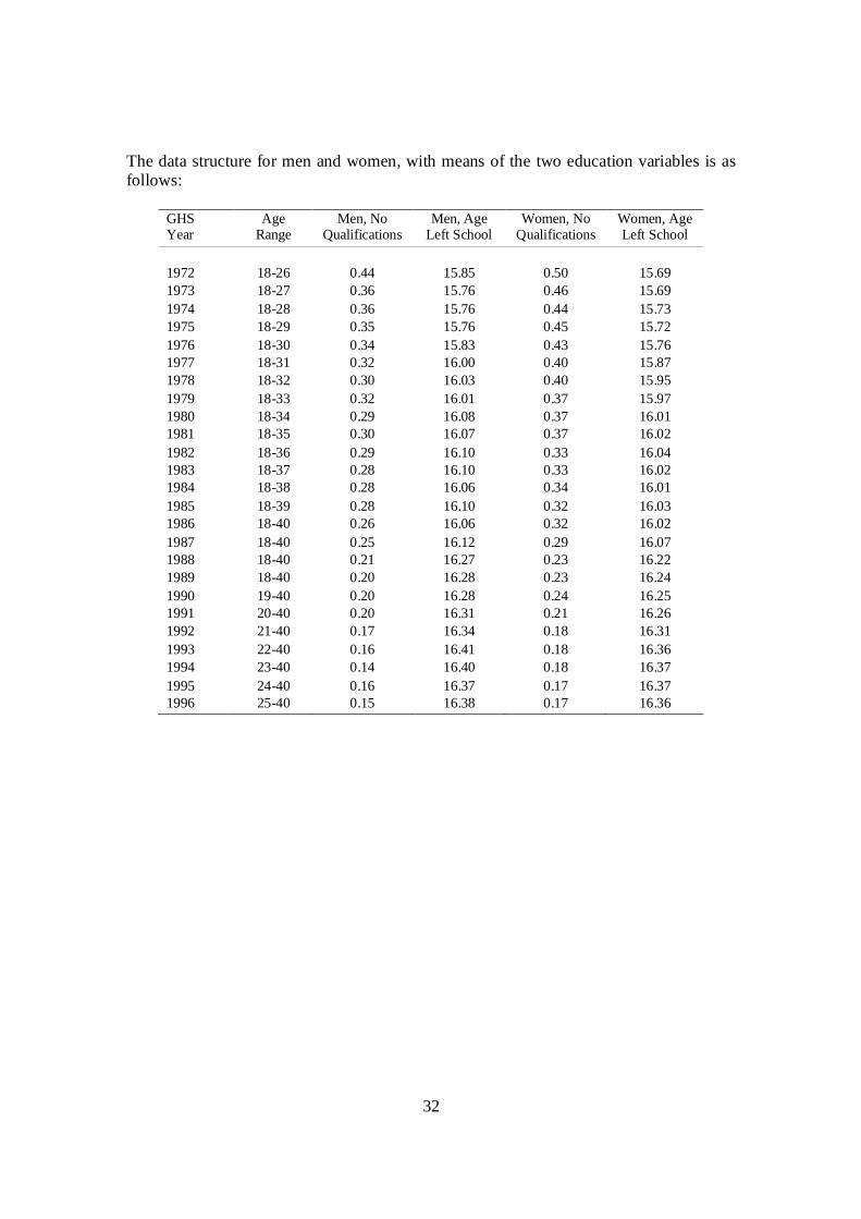
The data structure for men and women, with means of the two education variables is asfollows:
GHSYear
AgeRange
Men, NoQualifications
Men, AgeLeft School
Women, NoQualifications
Women, AgeLeft School
1972 18-26 0.44 15.85 0.50 15.691973 18-27 0.36 15.76 0.46 15.691974 18-28 0.36 15.76 0.44 15.731975 18-29 0.35 15.76 0.45 15.721976 18-30 0.34 15.83 0.43 15.761977 18-31 0.32 16.00 0.40 15.871978 18-32 0.30 16.03 0.40 15.951979 18-33 0.32 16.01 0.37 15.971980 18-34 0.29 16.08 0.37 16.011981 18-35 0.30 16.07 0.37 16.021982 18-36 0.29 16.10 0.33 16.041983 18-37 0.28 16.10 0.33 16.021984 18-38 0.28 16.06 0.34 16.011985 18-39 0.28 16.10 0.32 16.031986 18-40 0.26 16.06 0.32 16.021987 18-40 0.25 16.12 0.29 16.071988 18-40 0.21 16.27 0.23 16.221989 18-40 0.20 16.28 0.23 16.241990 19-40 0.20 16.28 0.24 16.251991 20-40 0.20 16.31 0.21 16.261992 21-40 0.17 16.34 0.18 16.311993 22-40 0.16 16.41 0.18 16.361994 23-40 0.14 16.40 0.18 16.371995 24-40 0.16 16.37 0.17 16.371996 25-40 0.15 16.38 0.17 16.36

33
Appendix BTable B1: The Causal Effect of Education on Crime, by Broad Types of Crime, Women
Women, Aged 18-40, Born 1946-70, Discontinuity Sample
Log(Property Convictions per 1000 Population) Log(Violent Convictions per 1000 Population)
A. Population Weighted No Qualifications Age Left School No Qualifications Age Left School(1)
CrimeReduced
Form
(2)EducationReduced
Form
(3)Crime
StructuralForm
(4)EducationReduced
Form
(5)Crime
StructuralForm
(6)Crime
ReducedForm
(7)EducationReduced
Form
(8)Crime
StructuralForm
(9)EducationReduced
Form
(10)Crime
StructuralForm
School Leaving Age Increase -0.017(0.064)
-0.168(0.019)
0.363(0.038)
-0.261(0.263)
-0.168(0.019)
0.363(0.038)
No Qualifications 0.106(0.382)
1.557(1.594)
Age Left School -0.049(0.177)
-0.719(0.740)
F-testF(1,117)
=0.08[P=.781]
F(1,117)=80.27
[P=.000]
F(1,117)=89.20
[P=.000]
F(1,117)=0.98
[P=.324]
F(1,117)=80.27
[P=.000]
F(1,117)=89.20
[P=.000]B. Inverse Distance Weighted No Qualifications Age Left School No Qualifications Age Left School
(1)Crime
ReducedForm
(2)EducationReduced
Form
(3)Crime
StructuralForm
(4)EducationReduced
Form
(5)Crime
StructuralForm
(6)Crime
ReducedForm
(7)EducationReduced
Form
(8)Crime
StructuralForm
(4)EducationReduced
Form
(10)Crime
StructuralForm
School Leaving Age Increase -0.017(0.063)
-0.185(0.019)
0.430(0.039)
-0.242(0.267)
-0.185(0.019)
0.430(0.039)
No Qualifications 0.092(0.338)
1.311(1.461)
Age Left School -0.039(0.146)
-0.563(0.632)
F-testF(1,117)
=0.07[P=.787]
F(1,117)=92.73
[P=.000]
F(1,117)=120.79[P=.000]
F(1,117)=0.82
[P=.366]
F(1,117)=92.73
[P=.000]
F(1,117)=120.79[P=.000]
Notes: As for Table 2. All specifications include a full set of age and year dummies and control variables. Sample size is 169 in all cases.