Embed Size (px)
Citation preview

The creep behaviour of adhesives A numerical and experimental investigation
Master’s Thesis in the International Master’s Programme Structural Engineering
MIGUEL MIRAVALLES
IIP DHARMAWAN Department of Civil and Environmental Engineering Division of Structural Engineering Steel and Timber Structures CHALMERS UNIVERSITY OF TECHNOLOGY Göteborg, Sweden 2007 Master’s Thesis 2007:110
0
0,05
0,1
0,15
0,2
0,25
0,3
0,35
0,4
0,45
0,5
0 500000 1000000 1500000 2000000 2500000 3000000
Time (s)
Cre
ep s
trai
n
Specimen 1 - 7.5 MPa
Specimen 2 - 7.8 MPa
Specimen 3 - 7 MPa
Specimen 4 - 16.8 MPa
Specimen 5 - 16.6 MPa


MASTER’S THESIS 2007:110
The creep behaviour of adhesives
A numerical and experimental investigation
Master’s Thesis in the International Master’s Programme Structural Engineering
MIGUEL MIRAVALLES
IIP DHARMAWAN
Department of Civil and Environmental Engineering Division of Structural Engineering
Steel and Timber Structures CHALMERS UNIVERSITY OF TECHNOLOGY
Göteborg, Sweden 2007
The creep behaviour of adhesives A numerical and experimental investigation
Master’s Thesis in the International Master’s Programme Structural Engineering
MIGUEL MIRAVALLES IIP DHARMAWAN
© MIGUEL MIRAVALLES
IIP DHARMAWAN, 2007
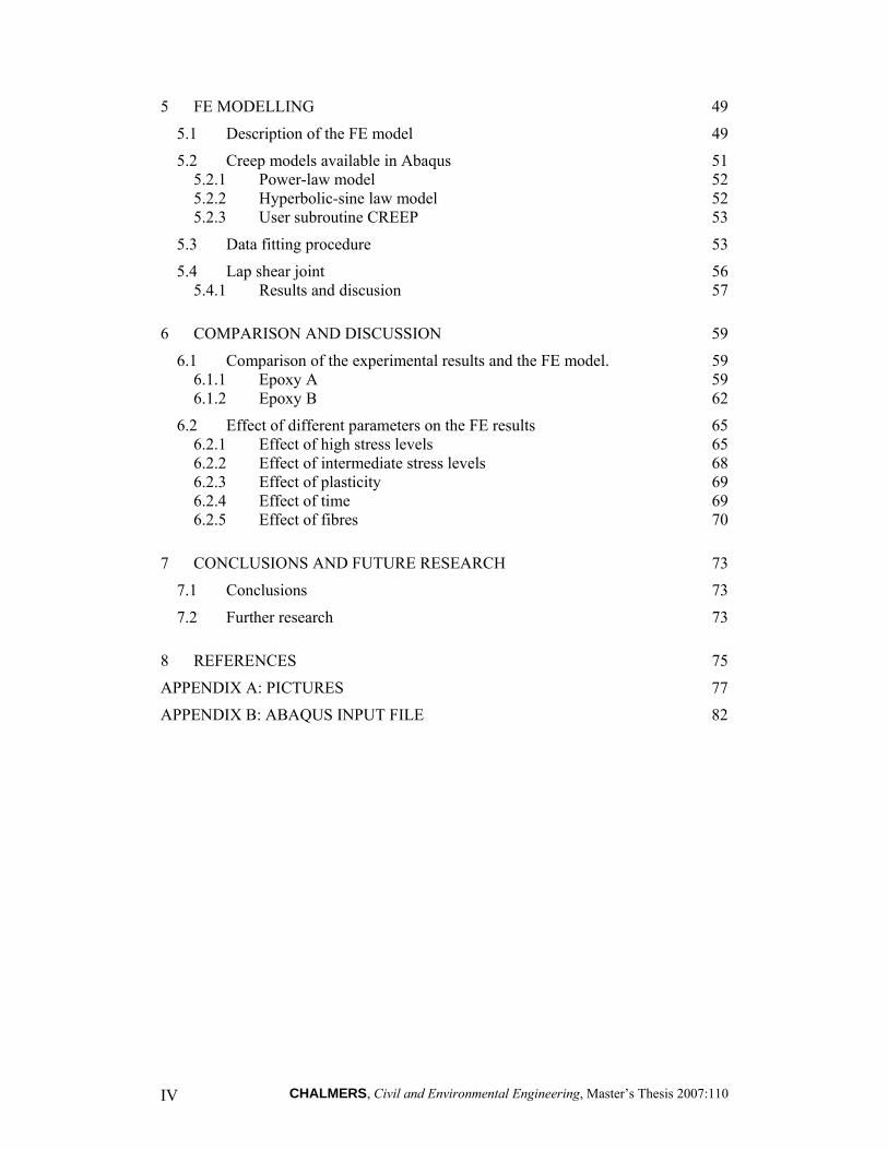
Master’s Thesis 2007:110 Department of Civil and Environmental Engineering Division of Structural Engineering Steel and Timber Structures Chalmers University of Technology SE-412 96 Göteborg Sweden Telephone: + 46 (0)31-772 1000 Cover: Figures 4.1 and 4.7: Creep test specimen dimensions and creep strain-time curve for all Epoxy A adhesive specimens reinforced with 0.5% carbon fibres. Chalmers repro service / Department of Civil and Environmental Engineering Göteborg, Sweden 2007
I
The creep behaviour of adhesives A numerical and experimental investigation
Master’s Thesis in the International Master’s Programme Structural Engineering
MIGUEL MIRAVALLES
IIP DHARMAWAN Department of Civil and Environmental Engineering Division of Structural Engineering Steel and Timber Structures Chalmers University of Technology ABSTRACT
The use of adhesives in the reinforcement of structural members has increased in the last few years. However, limited information concerning the creep behaviour of structural adhesives has been found in the literature. The present study is part of a general research project at Chalmers University of Technology focused on the strengthening of steel members with carbon fibre reinforced polymers (CFRP) and bonded by structural adhesives. This thesis specifically focuses on the analysis of the creep behaviour of structural adhesives and also the possibility to reinforce them with carbon fibres.
The present study includes uniaxial tensile creep tests, where two epoxy adhesives were tested at different stress levels. Experimental data showed that the adhesives reinforced with carbon fibres experiment less creep strains than the unreinforced adhesives. Uniaxial tensile tests were also performed in order to obtain material parameters, such as ultimate tensile stress, ultimate tensile strain, Young’s modulus and Poisson’s ratio. Non linear behaviour was observed and the results were in agreement with previous studies and the manufacturer’s data. No conclusions concerning the effect of fibre reinforcement could be made on tensile strength due to the scatter in the results.
It was found that much care should be given in the application of the adhesive during the performance of the tests because of air bubbles. Another factor that affected the results was that the orientation of the carbon fibres could not be controlled and they were randomly oriented.
A two-dimensional FE Model was developed based on the results from the tests in order to have a reliable tool to simulate the creep behaviour of adhesives. Results were compared with the experimental data, showing good agreement if high stresses were not considered.
As a suggestion for further research, a lap shear joint was also modelled using the constants obtained from the experiments. Results showed shear and peel stress redistribution in the adhesive layer.
Key words: creep, epoxy, adhesive, carbon fiber, reinforcement, time hardening, redistribution

II
CHALMERS Civil and Environmental Engineering, Master’s Thesis 2007:110 III
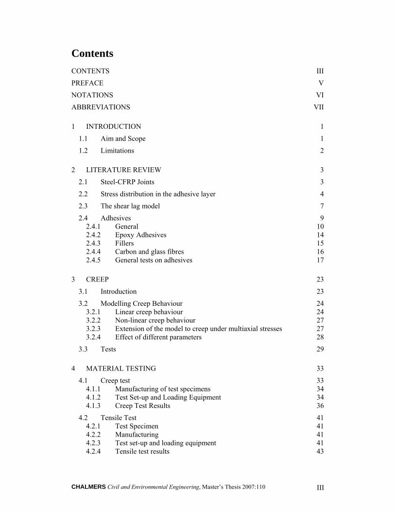
Contents CONTENTS III
PREFACE V
NOTATIONS VI
ABBREVIATIONS VII
1 INTRODUCTION 1
1.1 Aim and Scope 1
1.2 Limitations 2
2 LITERATURE REVIEW 3
2.1 Steel-CFRP Joints 3
2.2 Stress distribution in the adhesive layer 4
2.3 The shear lag model 7
2.4 Adhesives 9 2.4.1 General 10 2.4.2 Epoxy Adhesives 14 2.4.3 Fillers 15 2.4.4 Carbon and glass fibres 16 2.4.5 General tests on adhesives 17
3 CREEP 23
3.1 Introduction 23
3.2 Modelling Creep Behaviour 24 3.2.1 Linear creep behaviour 24 3.2.2 Non-linear creep behaviour 27 3.2.3 Extension of the model to creep under multiaxial stresses 27 3.2.4 Effect of different parameters 28
3.3 Tests 29
4 MATERIAL TESTING 33
4.1 Creep test 33 4.1.1 Manufacturing of test specimens 34 4.1.2 Test Set-up and Loading Equipment 34 4.1.3 Creep Test Results 36
4.2 Tensile Test 41 4.2.1 Test Specimen 41 4.2.2 Manufacturing 41 4.2.3 Test set-up and loading equipment 41 4.2.4 Tensile test results 43
CHALMERS, Civil and Environmental Engineering, Master’s Thesis 2007:110 IV
5 FE MODELLING 49
5.1 Description of the FE model 49
5.2 Creep models available in Abaqus 51 5.2.1 Power-law model 52 5.2.2 Hyperbolic-sine law model 52 5.2.3 User subroutine CREEP 53
5.3 Data fitting procedure 53
5.4 Lap shear joint 56 5.4.1 Results and discusion 57
6 COMPARISON AND DISCUSSION 59
6.1 Comparison of the experimental results and the FE model. 59 6.1.1 Epoxy A 59 6.1.2 Epoxy B 62
6.2 Effect of different parameters on the FE results 65 6.2.1 Effect of high stress levels 65 6.2.2 Effect of intermediate stress levels 68 6.2.3 Effect of plasticity 69 6.2.4 Effect of time 69 6.2.5 Effect of fibres 70
7 CONCLUSIONS AND FUTURE RESEARCH 73
7.1 Conclusions 73
7.2 Further research 73
8 REFERENCES 75
APPENDIX A: PICTURES 77
APPENDIX B: ABAQUS INPUT FILE 82

CHALMERS Civil and Environmental Engineering, Master’s Thesis 2007:110 V
Preface This project work was carried out as a final project of a Master of Science degree in the Department of Structural Engineering and Mechanics, Steel and Timber Structures at Chalmers University of Technology, Göteborg, Sweden.
The project was supervised and examined by Mohammad Al-Emrani. The working period was from February 2007 to October 2007. This project was part of a general research project at Chalmers University of Technology focused on the strengthening of steel members with carbon fibre reinforced polymers (CFRP) and bonded by structural adhesives.
We would like to thank our supervisor and also research student Reza Haghani for their guidance during the working period without which the project would have not been possible. We would like to thank as well those that have made important contributions and also influenced the work project. Important thanks as well for the companies which provided the epoxies and laminates necessary to carry out this study.
We also would like to thank the staff at the Department, which directly or indirectly gave their support and friendship during the project work period.
Göteborg October 2007
Miguel Miravalles
Iip Dharmawan

CHALMERS, Civil and Environmental Engineering, Master’s Thesis 2007:110 VI
Notations A Area, Creep constant D Compliance Do Instantaneous compliance E Young’s modulus K Parameter that controls the shape of the yield surface in the deviatoric
plane M0, M1 Data fitting constants R Universal gas constant Tg Transition temperature d Material cohesion stress m Creep constant n Creep constant p Hydrostatic component of the stress tensor, von Misses equivalent stress q~ Uniaxial equivalent deviatoric stress r Third invariant of the deviatoric stress tf Time to fracture to Mean relaxation time ΔH Activation energy β Material angle of friction γSV Interfacial tension of the solid material in equilibrium with a fluid vapour γLV Surface tension of the fluid material in equilibrium with its vapour γSL Interfacial tension between the solid and liquid materials ε Strain εult.paralel Ultimate strain in the parallel direction
CHALMERS Civil and Environmental Engineering, Master’s Thesis 2007:110 VII
εult.perpend Ultimate strain in the perpendicular direction
crε& Uniaxial equivalent creep strain rate η Viscosity of the material θ Contact angle, Temperature θZ User-defined value of absolute zero on the temperature scale μt Pressure sensitivity of the adhesive μm Yield envelope in the shape of a circular cone ν Poisson’s ratio σ1, σ2, σ3 Stresses in the different direction σult Ultimate tensile stress σe Effective shear stress σm Hydrostatic component of the creep stress τmax Critical maximum shear stress τ1 Relaxation time τ0 Yield stress in pure shear τm Von Misses yield stress τp Tresca stress
Abbreviations ASTM American Society for Testing and Materials CFRP Carbon Fibre Reinforced Polymer ISO International Organization for Standardization TAST Thick Adherend Shear Test


CHALMERS, Civil and Environmental Engineering, Master’s Thesis 2007:110 I

CHALMERS, Civil and Environmental Engineering, Master’s Thesis 2007:110 1
1 Introduction Carbon fibre reinforced polymers (CFRPs) are being used as reinforcing elements in a wide variety of constructions both in the case of rehabilitation and structural upgrading of existing structures. Design guidelines already exist in several countries and provide adequate information to use these materials with confidence in the case of concrete and masonry structures. In fact, several research studies have been developed on concrete and masonry structures and problems such as adhesion, interfacial stresses and debonding have been examined with sufficient accuracy. On the contrary, less attention has been dedicated to the use of CFRPs for the reinforcement of steel elements and the development of experimental research is still requested, especially on adhesives.
Epoxy-based structural adhesives have emerged as a critical component for bonding CFRPs with other materials due to their excellent adhesion properties, high mechanical strength and good chemical properties.
Structural adhesives are load-bearing materials with high modulus and strength that can transmit stress without loss of structural integrity. Compared with other joining methods, such as welding or bolting, epoxy-based structural adhesives provide exceptional advantages, including redistributing stresses equally over a large area while minimizing peak stress concentrations, joining dissimilar materials, and reducing the overall weight and manufacturing costs.
However, epoxy resins, being viscoelastic in nature, exhibit unique time-dependent behaviours. This leads to a great concern in assessing their long-term load-bearing performance, mainly because of a lack in fundamental knowledge on how creep affects the strength of adhesive joints. There is also a general concern regarding the lack of knowledge about the long-term performance of structural epoxy adhesives. Significant work is still required to develop accurate models for the prediction of the long term behaviour of epoxy adhesives, especially under different testing conditions.
Creep might be a serious problem when the stresses in the adhesive joint are relatively high, typically in strengthening steel structures with prestressed laminates.
Moreover, the reinforcement of these adhesives with fibres has never been studied and is an attractive field of research.
This report comprises the study of the long term behaviour of epoxy adhesives and is part of an ongoing research project that investigates the behaviour of steel-CFRP joints at Chalmers University of Technology.
1.1 Aim and Scope
The aim of this study is to examine the creep behaviour of two types of structural adhesives and the effect of reinforcing them with fibres. In order to do so, several creep tests were carried out on two different adhesives at different load levels.
Another objective of the study is to evaluate the available creep models in the commercial FE program Abaqus. Data from the tests was collected and used to get
CHALMERS, Civil and Environmental Engineering, Master’s Thesis 2007:110 2
parameters that were needed for the FE model and then results from the FE analysis were compared with the experimental results.
Chapter 2 of this report includes some background about steel-CFRP joints, general knowledge about adhesives and theories of adhesion.
Chapter 3 provides an overview of the creep phenomena on adhesives, showing some theoretical models and also explaining the different creep tests that can be carried out.
Chapter 4 explains the test procedure and presents the results.
Chapter 5 deals with the FE modelling of the epoxy adhesives.
Chapter 6 provides comparisons of the results obtained in the previous chapters.
Finally, Chapter 7 presents the conclusions of this study and recommendations for further studies.
1.2 Limitations
This study has been done in the frame of a master thesis, and has the following inherent limitations.
• The number of specimens tested was few, so the results lack good statistical control.
• Only the creep behaviour of the bulk adhesive was studied. The performance of bonded joints is not included in the study.
• The effect of different temperatures was not studied.Tests were only performed at room temperature
CHALMERS, Civil and Environmental Engineering, Master’s Thesis 2007:110 3
2 Literature Review
2.1 Steel-CFRP Joints
Carbon fibre reinforced polymers (CFRPs) are used as reinforcing elements in a wide variety of constructions both in the case of rehabilitation and structural upgrading of existing structures. In several countries, present guidelines provide assured information for the usage of adhesives to reinforce concrete and masonry structures. Many research studies have been conducted in the scope of reinforcing concrete with CFRP to examine and predict the developed interface stresses and problems with phenomena such as adhesion and debonding. On the contrary, less attention has been dedicated to the use of CFRPs for the reinforcement of steel elements and the development of experimental research is still requested.
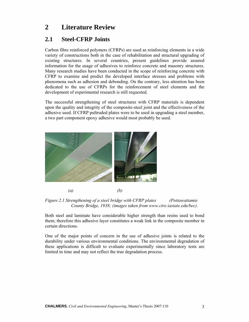
The successful strengthening of steel structures with CFRP materials is dependent upon the quality and integrity of the composite-steel joint and the effectiveness of the adhesive used. If CFRP pultruded plates were to be used in upgrading a steel member, a two part component epoxy adhesive would most probably be used.
(a) (b)
Figure 2.1 Strengthening of a steel bridge with CFRP plates (Pottawattamie County Bridge, 1938; (images taken from www.ctre.iastate.edu/bec).
Both steel and laminate have considerable higher strength than resins used to bond them; therefore this adhesive layer constitutes a weak link in the composite member in certain directions.
One of the major points of concern in the use of adhesive joints is related to the durability under various environmental conditions. The environmental degradation of these applications is difficult to evaluate experimentally since laboratory tests are limited in time and may not reflect the true degradation process.
CHALMERS, Civil and Environmental Engineering, Master’s Thesis 2007:110 4
Figure 2.2 Three-Point-Bending test on a steel beam reinforced with a CFRP plate. (Research Project conducted at the Dep. of Structural Engineering, Politecnico di Milano, Italy)
Irreversible damages of the bond may be caused by water due to the formation of oxides at the interface. Another detrimental effect can be the ultraviolet component of sunlight that can degrade the adhesive. Other important aspect that may affect the joint is the degradation of the material due to moisture absorption. A composite structure may also experience high temperatures such as fire conditions or high operating temperatures and, as a consequence, the mechanical performance of the adhesive may be seriously affected. Chapter 3 explains in further detail the effect of creep under some of these conditions.
2.2 Stress distribution in the adhesive layer
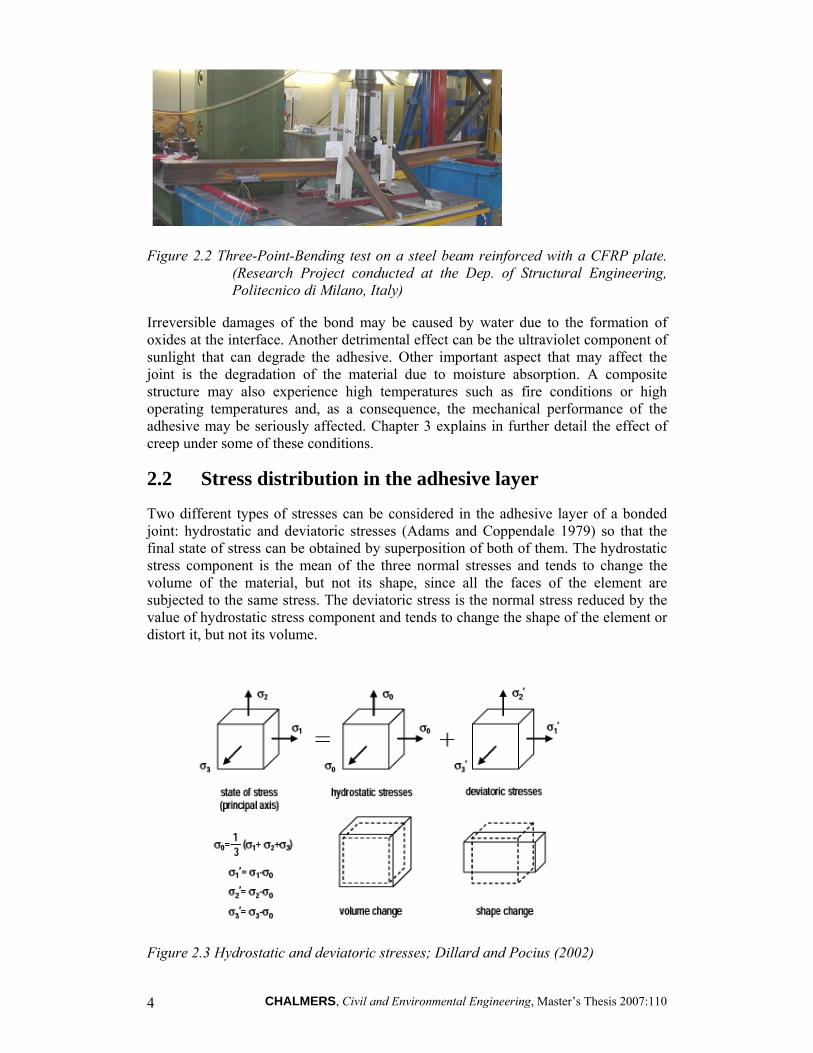
Two different types of stresses can be considered in the adhesive layer of a bonded joint: hydrostatic and deviatoric stresses (Adams and Coppendale 1979) so that the final state of stress can be obtained by superposition of both of them. The hydrostatic stress component is the mean of the three normal stresses and tends to change the volume of the material, but not its shape, since all the faces of the element are subjected to the same stress. The deviatoric stress is the normal stress reduced by the value of hydrostatic stress component and tends to change the shape of the element or distort it, but not its volume.
Figure 2.3 Hydrostatic and deviatoric stresses; Dillard and Pocius (2002)

CHALMERS, Civil and Environmental Engineering, Master’s Thesis 2007:110 5
Several criteria exist for modelling the yield behaviour of adhesives, but in many cases these criteria must be evaluated against the experimental data obtained in the tests in order to be sure that the model is reliable.
The standard criteria do not apply quantitatively to polymeric materials because they ignore the effect of the hydrostatic component of the stress tensor. Therefore, some modifications must be made and new expressions obtained. The most important ones are the modified Tresca, the modified von Mises, the Drucker-Prager citerion, and the modified Drucker-Prager/Cap citerion; see Wang (2000).
a) Modified Tresca yield criterion.
This model states that the critical maximum shear stress (τmax) is linearly dependent on the hydrostatic component of the stress tensor, p. The new, pressure-dependent Tresca criterion can be written as
ptμττ += 0max (2.1)
Where
( )31max 21 σστ −= (2.2)
3zyxp
σσσ ++−= (2.3)
with τ0 denoting the yield stress in pure shear, p the hydrostatic pressure, σ1 and σ3 the maximum and minimum principal stresses, and μt the pressure sensitivity of the adhesive. For constant values of μt , the yield envelope takes the shape of a hexagonal pyramid.
b) Modified von Mises yield criterion
The von Mises yield criterion can be modified in a similar way to the Tresca yield criterion in order to account for the hydrostatic components of the stress tensor. For instance, the yield criterion can be mathematically described as
pmmm μττ += 0 (2.4)
where τm denotes the von Misses yield stress, which is defined through the following equation:
( ) ( ) ( )213
232
221
26 σσσσσστ −+−+−=m (2.5)
and 0mτ is the yield stress in pure shear, while p is the hydrostatic component of the
stress tensor. As for the Tresca criterion, the parameter μm represents a yield envelope in the shape of a circular cone. An advantage over the Tresca criterion is that the von Mises yield surface/envelope (right circular cone) does not encounter the dicontinuities present on the Tresca yield surface/ envelope (hexagonal pyramid).
CHALMERS, Civil and Environmental Engineering, Master’s Thesis 2007:110 6
The stresses calculated based on the experimental results are substituted in Eqs. (11), (12) and (14), giving the Tresca stress τp, the hydrostatic pressure p, and the von Mises stress τm, respectively.
c) Drucker-Prager plasticity model
Due to the limitation of the modified von Mises yield criterion which implies that the shape of the yield surface in the deviatoric space is a sphere, the Drucker-Prager plasticity model has also been employed to model the yielding behaviour of porous materials. The equation for the Drucker-Prager yield surface is
0tan =−−= dptFs β (2.6)
where
⎥⎥⎦
⎤
⎢⎢⎣
⎡⎟⎟⎠
⎞⎜⎜⎝
⎛⎟⎠⎞
⎜⎝⎛ −−+=
31111
2 qr
kkqt (2.7)
23Jq = (2.8)
33
227 Jr ≡
( )( )( )2
222 213312321 σσσσσσσσσ ++++++= (2.9)
0tan311 cd σβ ⎟
⎠⎞
⎜⎝⎛ −= (2.10)
Here q is the von Mises equivalent stress and r is the third invariant of the deviatoric stress. The use of the deviatoric stress measure t is to allow the model to match different yield-stress values in tension and compression in the deviatoric plane. The constant β is the material angle of friction, d is the material cohesion stress, and the parameter K controls the shape of the yield surface in the deviatoric plane. The value of K is equal to the ratio of the flow stress in triaxial tension to the flow stress in triaxial compression. For example, K and β can be expressed in terms of the ratio of uniaxial compressive yield stress to uniaxial tensile yield stress )/( 00
tc σσλλ =
122
++
=λ
λK (2.11)
2)1(3tan
+−
=λλβ (2.12)
CHALMERS, Civil and Environmental Engineering, Master’s Thesis 2007:110 7
d) Modified Drucker-Prager/Cap plasticity model
Depending on the adhesive used, the three models discussed before might have a common deficiency: over-predicting the beneficial effect of compressive hydrostatic stress. In order to overcome this difficulty, the modified Drucker-Prager/Cap plasticity model can be adopted. The yield surface consists on three surfaces. The first one corresponds to predominantly shearing behaviour and is based on the Drucker-Prager model. The second one is a transition yield surface that has a constant radius in the meridional plane, ensuring the continuity of the overall yield locus. The last one is a “cap” yield surface which has en elliptical shape with constant eccentricity in the meridional plane. Hence, the three surfaces can be represented as:
0=sF , (2.13)
where Fs is given by Equation 2.6.
0=tF , (2.14)
with
( ) ( ) [ ]βαββ
β tantancos
cos2
2aaat pdpdatppF +−⎥
⎦
⎤⎢⎣
⎡+
−−+−= (2.15)
and
0=cF , (2.16)
( ) [ ]ββαα
tancos/1
22
aac pdRRtppF +−⎥⎦
⎤⎢⎣
⎡−+
+−= (2.17)
Having a look at the equations, this model consists of 6 different constants. All of them can be obtained by fitting the experimental data from tests to positive and negative hydrostatic pressure.
2.3 The shear lag model
The shear lag concept (Volkersen 1938) is of fundamental importance to any bonded configuration where load is transferred from one adherend to another, primarily through shear stresses within the adhesive layer (Dillard, Pocius 2003).
For any type of bonded joint involving adherends laid side by side and loaded axially in tension or compression the adhesive layer serves to transfer load from one adherend to the other through shear stresses distributed along the length of the bond.
The basics of the shear lag model proposed by Volkersen are:
CHALMERS, Civil and Environmental Engineering, Master’s Thesis 2007:110 8
• The adhesive does not carry any significant axial force, because it is more compliant in the axial direction than the adherends, and because it is relatively thin compared to the adherends.
• The adherends do not deform in shear, implying that the shear modulus of the adherends is much greater than that of the adhesive. This assumption becomes especially suspect with anisotropic materials such as wood- or fibre-reinforced composites.
• Out-of-plane normal stresses are ignored in both the adhesive and adherends.
• The effect of the load eccentricity or couple is ignored, and bending of the adherends is specifically ignored.
• Adhesive and adherends are assumed to behave in a linear elastic manner.
• Bonding is assumed to be perfect along both bond planes.
• The effects of the bond terminus are ignored.
• Plane stress conditions are assumed, ignoring complications arising from different Poisson contractions in the bonded region and single adherend regions.
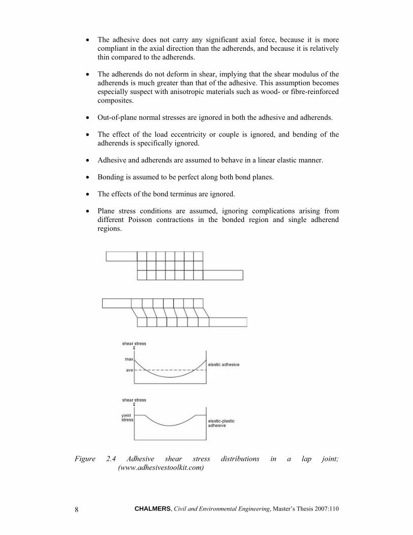
Figure 2.4 Adhesive shear stress distributions in a lap joint; (www.adhesivestoolkit.com)
CHALMERS, Civil and Environmental Engineering, Master’s Thesis 2007:110 9
When the joint is loaded, initially the adhesive is elastic, but for rigid adhesives on further loading the adhesive is stressed beyond its yield point in shear and regions of uniform stress develop at the edges of the joint. As the load is increased, these uniform shear regions will spread through the whole of the overlap and a limit will be reached when the joint can carry no further load.
The shear strains within the adhesive are seen to vary significantly along the length of the bond. A key feature to be gained from the Volkersen shear lag result is that there is a relatively uniform shear stress distribution only for the case of ‘short joints’. For longer joints, there are peaks in the shear stress anywhere there are relative changes in the stiffness of the adherends. Thus near joint ends, large shear stress peaks are expected.
2.4 Adhesives
Having a look back in history, adhesives appeared long time ago. Most of them were made of vegetable, mineral or animal substances. The first ones to use them were the early hunters, who bonded feathers to arrows with beeswax, in order to have better accuracy. In the palace of Knossos in Crete, the walls were painted with chalk, iron ocher and copper, which were binded with wet lime. About 3300 years ago, carvings in Thebes show a glue pot and brush to join a thin piece of veneer to a plank of sycamore. The Egyptians also used adhesives. They decorated wooden coffins with pigments that were bonded with a mixture of glue and chalk. It is thought that one of the most famous buildings in history, the Tower of Babel, was built with the aid of slime as mortar. In the days of Theophilus wooden objects were fixed with cheese, stag horns and fish glues.
The first commercial glue plant was founded in Holland in 1690. The real development of adhesives started well into the 20th century with the polymeric and elastomeric resins.
In Table 2.1 a summary of the most important products developed during the last century can be seen.
CHALMERS, Civil and Environmental Engineering, Master’s Thesis 2007:110 10
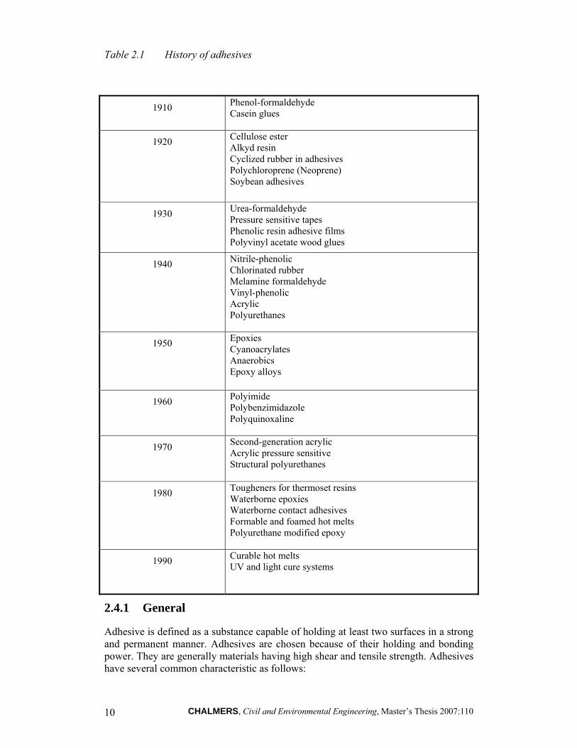
Table 2.1 History of adhesives
2.4.1 General
Adhesive is defined as a substance capable of holding at least two surfaces in a strong and permanent manner. Adhesives are chosen because of their holding and bonding power. They are generally materials having high shear and tensile strength. Adhesives have several common characteristic as follows:
1910 Phenol-formaldehyde Casein glues
1920
Cellulose ester Alkyd resin Cyclized rubber in adhesives Polychloroprene (Neoprene) Soybean adhesives
1930
Urea-formaldehyde Pressure sensitive tapes Phenolic resin adhesive films Polyvinyl acetate wood glues
1940
Nitrile-phenolic Chlorinated rubber Melamine formaldehyde Vinyl-phenolic Acrylic Polyurethanes
1950
Epoxies Cyanoacrylates Anaerobics Epoxy alloys
1960 Polyimide Polybenzimidazole Polyquinoxaline
1970
Second-generation acrylic Acrylic pressure sensitive Structural polyurethanes
1980
Tougheners for thermoset resins Waterborne epoxies Waterborne contact adhesives Formable and foamed hot melts Polyurethane modified epoxy
1990
Curable hot melts UV and light cure systems
CHALMERS, Civil and Environmental Engineering, Master’s Thesis 2007:110 11
• To form surface attachment through adhesion.
• To improve strength and improve bonding carrying capacity.
• To transfer and distribute load among the components in an assembly.
Adhesives can be classified into structural adhesives and non-structural adhesives. The term structural adhesive is used to define an adhesive whose strength is critical to the success of an assembly. This term is usually reserved to describe adhesives with high shear strength and good durability. Examples of these structural adhesives are epoxy, thermosetting acrylic, and urethane systems. Non-structural adhesives are adhesives with lower strength and permanence. They are usually used for temporary fastening or bonding weak substrates. Examples of non-structural adhesives are pressure sensitive film, wood glue, elastomers and sealants.
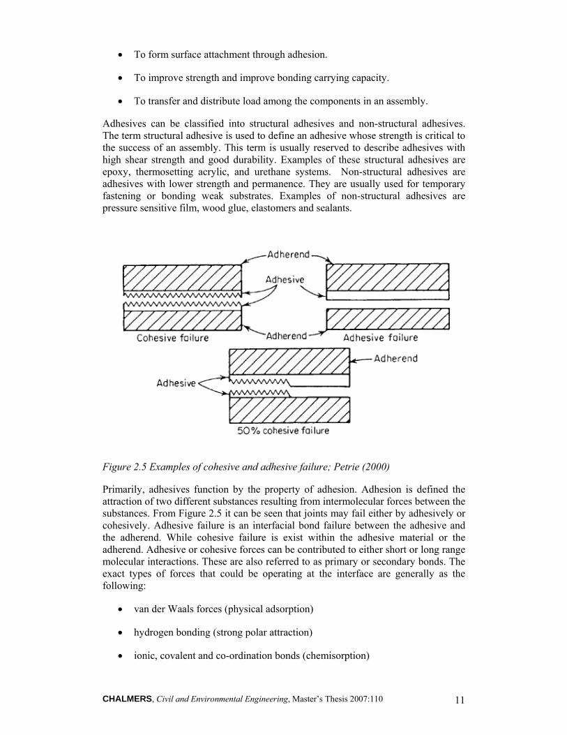
Figure 2.5 Examples of cohesive and adhesive failure; Petrie (2000)
Primarily, adhesives function by the property of adhesion. Adhesion is defined the attraction of two different substances resulting from intermolecular forces between the substances. From Figure 2.5 it can be seen that joints may fail either by adhesively or cohesively. Adhesive failure is an interfacial bond failure between the adhesive and the adherend. While cohesive failure is exist within the adhesive material or the adherend. Adhesive or cohesive forces can be contributed to either short or long range molecular interactions. These are also referred to as primary or secondary bonds. The exact types of forces that could be operating at the interface are generally as the following:
• van der Waals forces (physical adsorption)
• hydrogen bonding (strong polar attraction)
• ionic, covalent and co-ordination bonds (chemisorption)
CHALMERS, Civil and Environmental Engineering, Master’s Thesis 2007:110 12
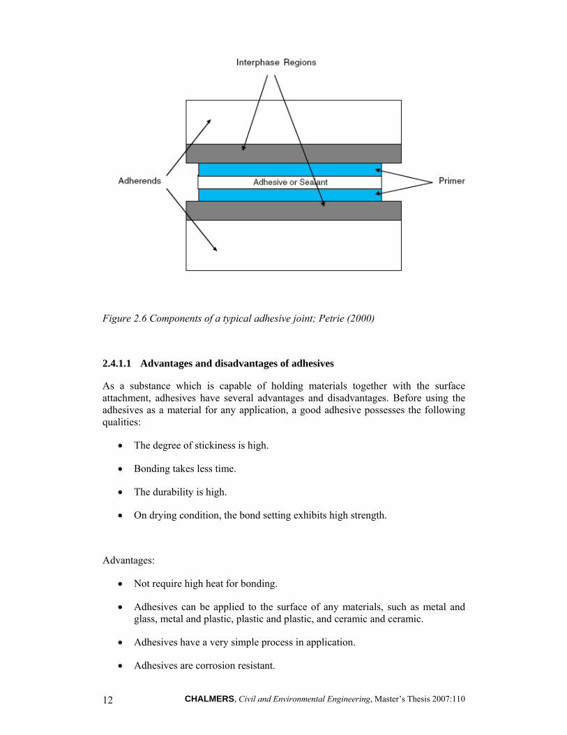
Figure 2.6 Components of a typical adhesive joint; Petrie (2000)
2.4.1.1 Advantages and disadvantages of adhesives
As a substance which is capable of holding materials together with the surface attachment, adhesives have several advantages and disadvantages. Before using the adhesives as a material for any application, a good adhesive possesses the following qualities:
• The degree of stickiness is high.
• Bonding takes less time.
• The durability is high.
• On drying condition, the bond setting exhibits high strength.
Advantages:
• Not require high heat for bonding.
• Adhesives can be applied to the surface of any materials, such as metal and glass, metal and plastic, plastic and plastic, and ceramic and ceramic.
• Adhesives have a very simple process in application.
• Adhesives are corrosion resistant.

CHALMERS, Civil and Environmental Engineering, Master’s Thesis 2007:110 13
• Adhesives joints are leak-proof for gases and liquids.
• Adhesives are electrical and thermal insulators.
• Adhesives provide excellent fatigue strength.
• Adhesives reduce and prevent galvanic corrosion along the joints of dissimilar metals, e.g., aluminium-to-paper, iron-to-copper.
• Bonding between surfaces occurs easily and quickly.
• Adhesives provide large-stress bearing area, leading to lighter and stronger assemblies which could not be achieved with mechanical fastening.
• Adhesives provide attractive strength-to-weight ratio.
• Adhesives provide smooth contours.
Disadvantages:
• Adhesives can not be applied at elevated temperature. The bond strength decreases rapidly with the rise in temperature.
• Adhesive strength is generally weak and fixation is not long lasting.
• There is no single general purpose adhesive that can be used to join all types of surfaces. Therefore, for a particular job a specific adhesive is required.
• Adhesives can be applied only on plain and clean surface.
• Adhesives are susceptible to high humidity.
• Adhesives do not develop their full bonding strength and performance immediately after application. As a result, adhesives require time for fixation and to gain their full strength.
• Inspection of finished joints is difficult.
• Environmental, health and safety consideration are necessary.
• Jigs and fixture may be needed.
• Rigid process control is usually necessary.
• Useful life depends on environment.
• Long curing time may be needed.
CHALMERS, Civil and Environmental Engineering, Master’s Thesis 2007:110 14
2.4.1.2 Adhesive classifications
In order to classify adhesives, there are many types and variations of commercial adhesive materials to choose from for any specific application. There are also an unlimited number of adhesive composition possibilities available to the formulator for the engineering of a custom product. The adhesives have been classified by many methods and there can be many classification schemes. The industry settled on several common methods of classifying adhesives that satisfy most purposes. These classifications are:
• Function
• Chemical composition
• Mode of application and reaction
• Physical form
• Cost
• End-use
2.4.2 Epoxy Adhesives
Nowadays more 50 different substances can be included in the definition for an epoxy resin. Considering that there are even more hardeners, the different types of epoxy adhesives that can be manufactured in order to fulfil any desired requirement is really big.
Some of their main properties are:
• Adhesion Epoxy has capacity to adhere to most substrates.
• Mechanical strength epoxy-based structural adhesives have a high modulus and strength. The tensile strength can exceed 80 MPa.
• Chemical resistance Epoxy is resistant to most chemicals, especially alkali.
• Diffusion density Epoxy generally has relatively high vapour transmission resistance, but with special technique it can be made open to diffusion.
• Water tightness Epoxy plastics are considered as watertight and are often used to protect against water.
• Electrical insulation capacity Epoxy plastics are excellent electrical insulators.
• Shrinkage Epoxy plastics have very slight shrinkage during hardening.
• Modifiable Unlimited capability to modify the final properties of epoxy plastic to meet special requirements.
CHALMERS, Civil and Environmental Engineering, Master’s Thesis 2007:110 15
• Stability in light Epoxy plastics based on aromatic epoxy resins are sensitive to light in the UV range. Direct light with ultraviolet light causes yellowing.
There is a wide range of application of epoxy plastics in Civil Engineering. Some of the fields where they can be used are: Impregnation in sealing, thin layer coatings, self-levelling coatings, epoxy concrete, concrete sealing, reinforcement of concrete construction, gluing of new concrete to old, repair material, injection and lamination
Many epoxy adhesives can be included in the group of structural adhesives, which can be defined as load-bearing materials with high modulus and strength that can transmit stress without loss of structural integrity. They have replaced both mechanical fasteners and welding techniques in many industrial applications. Their main advantages over the other joining techniques are:
• Elimination of stress point concentrations by even distribution of stress over the entire bonded surface, plus improved load bearing capacity.
• Weight reduction.
• Enhanced structural appearance because protrusions, punctures, and attachments are eliminated.
• Cost savings, including lower labour costs.
• Bonding of dissimilar materials. Often the adhesive bond line acts as an insulator against galvanic corrosion in metal assemblies.
• Improved fatigue resistance, and resistance to shock, vibration, and thermal cycling.
• Protective sealing against contamination by liquids or gases.
2.4.3 Fillers
Fillers are often used in adhesives in order to improve their properties, such as increasing hardness and to have reinforcing properties. Hence, the choice of the filler and its concentration are often critical. In addition, adhesion may also be affected by the filler's presence either due to absorption of coupling agents, change in rheological properties (reducing mechanical adhesion) or changing moisture permeability which affects hydrolytic changes at the interphase.
It has been shown that in pressure sensitive adhesives, fillers may affect properties such as cohesion, cold flow and peel adhesion. Most fillers increase cohesion and reduce cold flow; see Wypych (2000).
Fillers are usually used in epoxy adhesives for many different purposes. They can be used to increase thermal conductivity, improve corrosion resistance, reduce shrinkage during cure, and sometimes to reduce cost.
Some examples of fillers in epoxy adhesives are the ones used to increase wear resistance in thin layer coatings,

CHALMERS, Civil and Environmental Engineering, Master’s Thesis 2007:110 16
Some types of fillers which can modify epoxy adhesive properties are:
• Reinforcing fillers
• Glass fillers
• Corrosion-inhibiting fillers
• Adhesion-promoting fillers
• Cure-promoting fillers
• Electrical conductivity-promoting fillers
• Silica fillers
• Flow control fillers
There are some more examples of fillers in epoxy adhesives: wear resistance is increased in thin layer coatings by using hard filler; the so-called epoxy concrete is reinforced with quartz sand in order to stand higher mechanical stresses; when new concrete is glued to old, the epoxy adhesive contains filler that prevents a too powerful penetration of the glue.
According to Hughes and Rutherford (1979), who used Al2O3 as filler in different adhesives, the highest filled adhesive had the lowest creep rate, whereas the adhesive with the least amount of filler had the highest creep rate.
Therefore, the use of fibres in epoxy adhesives has been considered to be an interesting point that could improve the behaviour of bonded joints.
In the next section the basic properties of fibres are explained in further detail in order to get a brief idea of their response as filler material in epoxy adhesives.
2.4.4 Carbon and glass fibres
Carbon fibres
Carbon fibres exhibit outstanding properties. Their strength is similar to the strongest steels and their stiffness can be greater than any metal, ceramic or polymer; and they can exhibit thermal and electrical conductivities that greatly exceed those of the competing materials. Moreover, if the strength or stiffness values are divided by the low density, then their high specific properties make this class of materials quite unique.
They are generally used together with epoxy, where high strength and stiffness are required, i.e. race cars, automotive and space applications, sport equipment. According to this, it could be valid filler in an epoxy adhesive. The main problem is that carbon fibres are known to be electrically conductive. Hence, in the case of direct contact between carbon fibres and iron in the presence of an electrolyte such as seawater or de-icing salts, galvanic corrosion may cause rusting of metal and create blistering and debonding. Non-uniformities in the material accelerate the deterioration process leading to localised corrosion. The aim of this project is focused on the
CHALMERS, Civil and Environmental Engineering, Master’s Thesis 2007:110 17
application of these adhesives in steel structures such as bridges, so oxidation may reduce the cross-sectional area of the structural member and, as a result, the overall load-carrying capacity decreases.
Glass fibres
Glass fibres are also an interesting material that can be used to reinforce adhesives. One of their main properties is that they have a high tensile strength. Its strength to weight ratio exceeds steel in some applications. Due to their low coefficient of thermal linear expansion and high coefficient of thermal conductivity, they exhibit excellent performance in thermal environments. Glass fibres do not absorb water, so there is no oxidation problem between this and steel. They are non-conductive (good for electrical insulation). In contrast to carbon fibres, glass fibres can undergo more elongation before they break. Depending on the application, many different types of glass fibres can be used. Some of the most important are:
• E-glass: this fibre has good insulation properties and is the premium fibre used in the majority of textile fibreglass production. It is very strong, stiff, and temperature resistant.
• S-glass: based on magnesium and aluminium silicate, it is very strong (40% stronger than the E-glass type), stiff, and temperature resistant.
• A-glass and C-glass: both of them have good chemical resistance.
• R-glass: a special composition that is alkali resistant and is used in reinforcing concrete.
Buch (2000) studied the creep properties of an epoxy adhesive supported and non-supported by a net of glass fibres. The results showed that creep was diminished when the adhesive was supported by this net of glass fibres.
2.4.5 General tests on adhesives
To determine the stresses in a structural bonded joint and further to predict its strength in service life, it is necessary to know the material properties of adhesive and adherend. For a linear stress analysis, Young’s modulus and Poisson’s ratio are the two input data. For a material nonlinear analysis, stress-strain curves may be required and material yielding and hardening rules may also be needed.
Two different kinds of tests can be made. The first one is the characterization of bulk adhesive, where the properties are intrinsic to the adhesive and not influenced by the adherends. They can be tested in uniaxial tension or compression, flexion and torsion. The testing of bulk specimens is easy because the elastic deformations are larger and can therefore be measured more accurately using standard extensometers or strain gauges. The other kind of test is the determination of in-situ adhesive properties in the joint, where the adhesive layer is in a complex state of stress.
Although it can be thought that the results obtained from each test will differ a lot, it has been demonstrated that there is a good correlation between the adhesive properties in bulk and the ones in the joint. Adams and Coppendale (1977), Jeandrau (1986; 1991) showed that the layer and bulk mechanical properties are similar under the
CHALMERS, Civil and Environmental Engineering, Master’s Thesis 2007:110 18
same curing conditions. The problem is to provide the same curing conditions for bulk and layer because of runaway exothermic reactions in bulk forms, which can explain discrepancies. Thus, the estimation made with bulk properties could differ from adhesive joint behaviour because of differences in operating environment. The most difficult part is to manufacture specimens without defects such as voids and porosity since air bubbles trapped during mixing are difficult to remove if the adhesive is very viscous or has a short pot-life.
There are many different test methods available to characterize the behaviour of joints. Acceptable test methods are published in the ASTM standards (American Society of testing materials), the BS standards (British standards), and the ISO standards (International Standards Organization)
2.4.5.1 Bulk tests
Deformations of bulk specimens are easily measured using standard extensometers or strain gauges. The main difficulty is to produce specimens without defects such as voids and porosity.
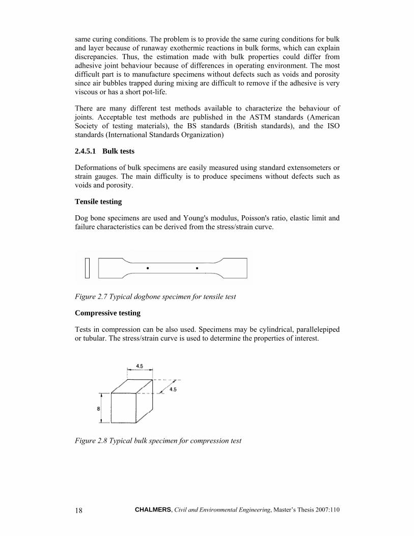
Tensile testing
Dog bone specimens are used and Young's modulus, Poisson's ratio, elastic limit and failure characteristics can be derived from the stress/strain curve.
Figure 2.7 Typical dogbone specimen for tensile test
Compressive testing
Tests in compression can be also used. Specimens may be cylindrical, parallelepiped or tubular. The stress/strain curve is used to determine the properties of interest.
Figure 2.8 Typical bulk specimen for compression test
CHALMERS, Civil and Environmental Engineering, Master’s Thesis 2007:110 19
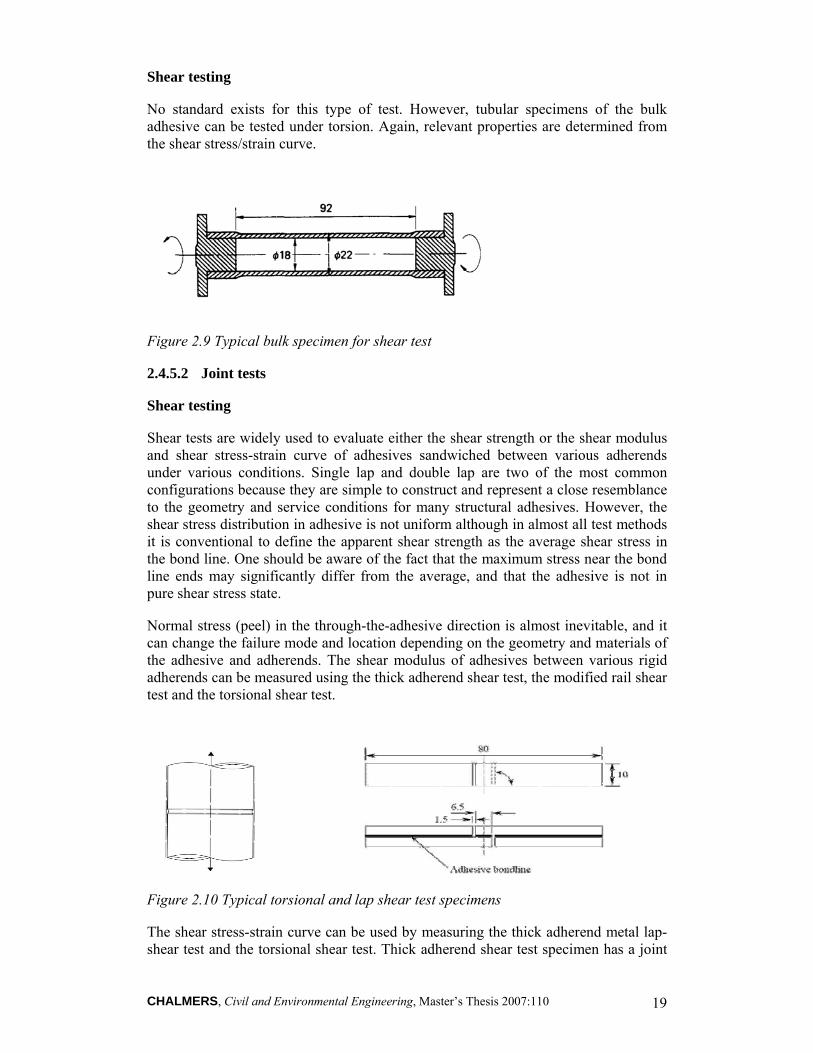
Shear testing
No standard exists for this type of test. However, tubular specimens of the bulk adhesive can be tested under torsion. Again, relevant properties are determined from the shear stress/strain curve.
Figure 2.9 Typical bulk specimen for shear test
2.4.5.2 Joint tests
Shear testing
Shear tests are widely used to evaluate either the shear strength or the shear modulus and shear stress-strain curve of adhesives sandwiched between various adherends under various conditions. Single lap and double lap are two of the most common configurations because they are simple to construct and represent a close resemblance to the geometry and service conditions for many structural adhesives. However, the shear stress distribution in adhesive is not uniform although in almost all test methods it is conventional to define the apparent shear strength as the average shear stress in the bond line. One should be aware of the fact that the maximum stress near the bond line ends may significantly differ from the average, and that the adhesive is not in pure shear stress state.
Normal stress (peel) in the through-the-adhesive direction is almost inevitable, and it can change the failure mode and location depending on the geometry and materials of the adhesive and adherends. The shear modulus of adhesives between various rigid adherends can be measured using the thick adherend shear test, the modified rail shear test and the torsional shear test.
Figure 2.10 Typical torsional and lap shear test specimens
The shear stress-strain curve can be used by measuring the thick adherend metal lap-shear test and the torsional shear test. Thick adherend shear test specimen has a joint
CHALMERS, Civil and Environmental Engineering, Master’s Thesis 2007:110 20
geometry simpler than the torsional shear specimen, and thus can be more easily made.
For joining fibre-reinforced plastics (FRP) and metals, ASTM D5868-95 describes a lap shear test for use in measuring the bonding characteristics of the adhesive. This test method is also applicable to random fibre oriented FRP. In addition, ASTM D5573-94 details the standard practice and method for classifying, identifying, and characterizing the failure modes in adhesively bonded fibre-reinforced-plastic (FRP) joints.
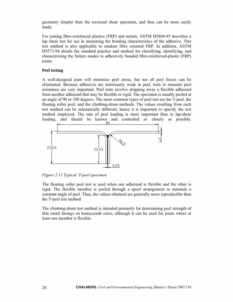
Peel testing
A well-designed joint will minimize peel stress, but not all peel forces can be eliminated. Because adhesives are notoriously weak in peel, tests to measure peel resistance are very important. Peel tests involve stripping away a flexible adherend from another adherend that may be flexible or rigid. The specimen is usually peeled at an angle of 90 or 180 degrees. The most common types of peel test are the T-peel, the floating roller peel, and the climbing-drum methods. The values resulting from each test method can be substantially different; hence it is important to specify the test method employed. The rate of peel loading is more important than in lap-shear loading, and should be known and controlled as closely as possible.
Figure 2.11 Typical T-peel specimen
The floating roller peel test is used when one adherend is flexible and the other is rigid. The flexible member is peeled through a spool arrangement to maintain a constant angle of peel. Thus, the values obtained are generally more reproducible than the T-peel test method.
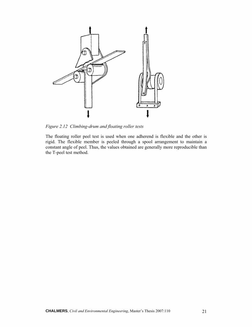
The climbing-drum test method is intended primarily for determining peel strength of thin metal facings on honeycomb cores, although it can be used for joints where at least one member is flexible.
CHALMERS, Civil and Environmental Engineering, Master’s Thesis 2007:110 21
Figure 2.12 Climbing-drum and floating roller tests
The floating roller peel test is used when one adherend is flexible and the other is rigid. The flexible member is peeled through a spool arrangement to maintain a constant angle of peel. Thus, the values obtained are generally more reproducible than the T-peel test method.

CHALMERS, Civil and Environmental Engineering, Master’s Thesis 2007:110 22
CHALMERS, Civil and Environmental Engineering, Master’s Thesis 2007:110 23
3 Creep
3.1 Introduction
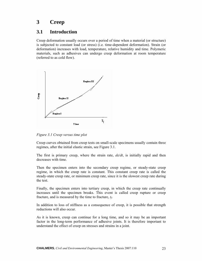
Creep deformation usually occurs over a period of time when a material (or structure) is subjected to constant load (or stress) (i.e. time-dependent deformation). Strain (or deformation) increases with load, temperature, relative humidity and time. Polymeric materials, such as adhesives can undergo creep deformation at room temperature (referred to as cold flow).
Figure 3.1 Creep versus time plot
Creep curves obtained from creep tests on small-scale specimens usually contain three regimes, after the initial elastic strain, see Figure 3.1.
The first is primary creep, where the strain rate, dε/dt, is initially rapid and then decreases with time.
Then the specimen enters into the secondary creep regime, or steady-state creep regime, in which the creep rate is constant. This constant creep rate is called the steady-state creep rate, or minimum creep rate, since it is the slowest creep rate during the test.
Finally, the specimen enters into tertiary creep, in which the creep rate continually increases until the specimen breaks. This event is called creep rupture or creep fracture, and is measured by the time to fracture, tf.
In addition to loss of stiffness as a consequence of creep, it is possible that strength reductions will also occur.
As it is known, creep can continue for a long time, and so it may be an important factor in the long-term performance of adhesive joints. It is therefore important to understand the effect of creep on stresses and strains in a joint.
CHALMERS, Civil and Environmental Engineering, Master’s Thesis 2007:110 24
It has been shown by some finite element works (Su, 1992) that the effect of creep is to reduce the shear stress concentrations in a TAST specimen, but not a very large amount. The normal stresses along the central line of the adhesive layer even out and for an adhesive with strong creep behaviour will tend to zero. Perhaps, more significantly, the peak normal stress at the interface is also significantly reduced. The amount of this reduction seems to be less dependent on the creep properties of the adhesives. However, this reduction in peak normal stress is also associated with an increase in peak normal strain at the interface, and the amount of this increase is strongly related to the creep properties of the adhesive.
This study also concluded that although the shear stresses are not much changed, the shear strains do increase significantly, and the size of this increase is strongly related to the creep properties of the adhesive. It is also pointed that the decrease in peak normal stress and increase in shear strain are occur simultaneously, so there may be a period when the reduction in normal stress leads to increased failure load, but later the increased shear strain will lead to failure at a lower load. This increase in shear strain means that despite the reduction in peak normal stress it is probable that an adhesive that is going to perform well in the long term should not have very strong creep behaviour.
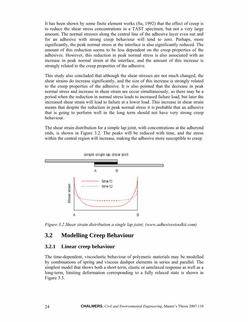
The shear strain distribution for a simple lap joint, with concentrations at the adherend ends, is shown in Figure 3.2. The peaks will be reduced with time, and the stress within the central region will increase, making the adhesive more susceptible to creep.
Figure 3.2 Shear strain distribution a single lap joint; (www.adhesivestoolkit.com)
3.2 Modelling Creep Behaviour
3.2.1 Linear creep behaviour
The time-dependent, viscoelastic behaviour of polymeric materials may be modelled by combinations of spring and viscous dashpot elements in series and parallel. The simplest model that shows both a short-term, elastic or unrelaxed response as well as a long-term, limiting deformation corresponding to a fully relaxed state is shown in Figure 3.3.
CHALMERS, Civil and Environmental Engineering, Master’s Thesis 2007:110 25
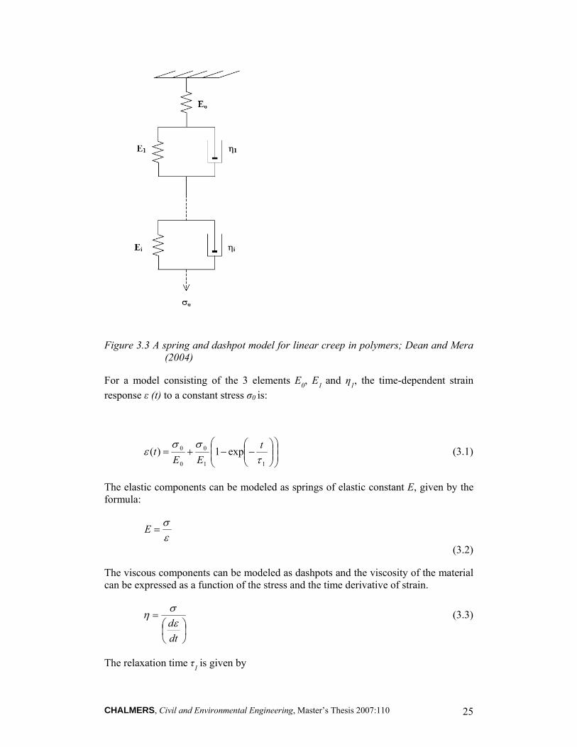
Figure 3.3 A spring and dashpot model for linear creep in polymers; Dean and Mera (2004)
For a model consisting of the 3 elements E0, E1 and η1, the time-dependent strain response ε (t) to a constant stress σ0 is:
⎟⎟⎠
⎞⎜⎜⎝
⎛⎟⎟⎠
⎞⎜⎜⎝
⎛−−+=
11
0
0
0 exp1)(τ
σσε t
EEt (3.1)
The elastic components can be modeled as springs of elastic constant E, given by the formula:
εσ
=E
(3.2)
The viscous components can be modeled as dashpots and the viscosity of the material can be expressed as a function of the stress and the time derivative of strain.
⎟⎠⎞
⎜⎝⎛
=
dtdεση (3.3)
The relaxation time τ1 is given by
CHALMERS, Civil and Environmental Engineering, Master’s Thesis 2007:110 26
1
11 E
ητ = (3.4)
This single relaxation time model will not describe actual relaxation processes in polymers which have a very broad distribution of relaxation times. Figure 3.3 can be extended, through the incorporation of additional spring and dashpot (Voigt) elements in series to broaden the spectrum of relaxation times and hence the time span of the relaxation process being modelled. The strain response now to an applied stress is
⎟⎟⎠
⎞⎜⎜⎝
⎛⎟⎟⎠
⎞⎜⎜⎝
⎛−−+= ∑
= i
n
i
tEE
tτ
σσ
ε exp11)(1 1
00
0 (3.5)
where there are n Voigt elements in the model.
The large number of parameters that need to be determined in this model is inconvenient and is usually not necessary for modelling creep in glassy polymers at temperatures well below the glass-to-rubber transition temperature, Dean and Mera (2004). Creep strains can then be described by the more simple expression
m
tt
Et ⎟⎟
⎠
⎞⎜⎜⎝
⎛−=
00
0 exp)(σ
ε (3.6)
This function will only model the short-time tail of the relaxation function given by equation (3.5), but this is usually a valid approximation, even for extended periods under load, as long as the measurement temperature is not close to the glass transition temperature. In equation (3.6), the exponent m characterises a broad spectrum of relaxation times whose mean or effective value is to. The equation can also be expressed as a creep compliance function D(t) where
m
t
ttDtD ⎟⎟⎠
⎞⎜⎜⎝
⎛==
00
0
exp)(σε
(3.7)
where Do is the instantaneous compliance of the material. Compliance can be defined as the inverse of the stiffness.
The magnitude of the parameter to depends on temperature, stress level and stress state. The magnitude of to also depends on the state of physical ageing of the adhesive at the time of the creep loading.
⎟⎟
⎠
⎞
⎜⎜
⎝
⎛
⎥⎥⎦
⎤
⎢⎢⎣
⎡⎟⎟⎠
⎞⎜⎜⎝
⎛−−Δ+=
m
ttDDtD0
0 exp1)( (3.8)
Where 0t can be expressed as:
μeBtt =0 (3.9)
CHALMERS, Civil and Environmental Engineering, Master’s Thesis 2007:110 27
et is defined as ageing time
B and μ are material constants obtained from experimental data
The creep tests carried out in this work did not have a too long duration, so changes in t0 due to physical ageing will be small and these effects can be neglected in the analysis of creep behaviour.
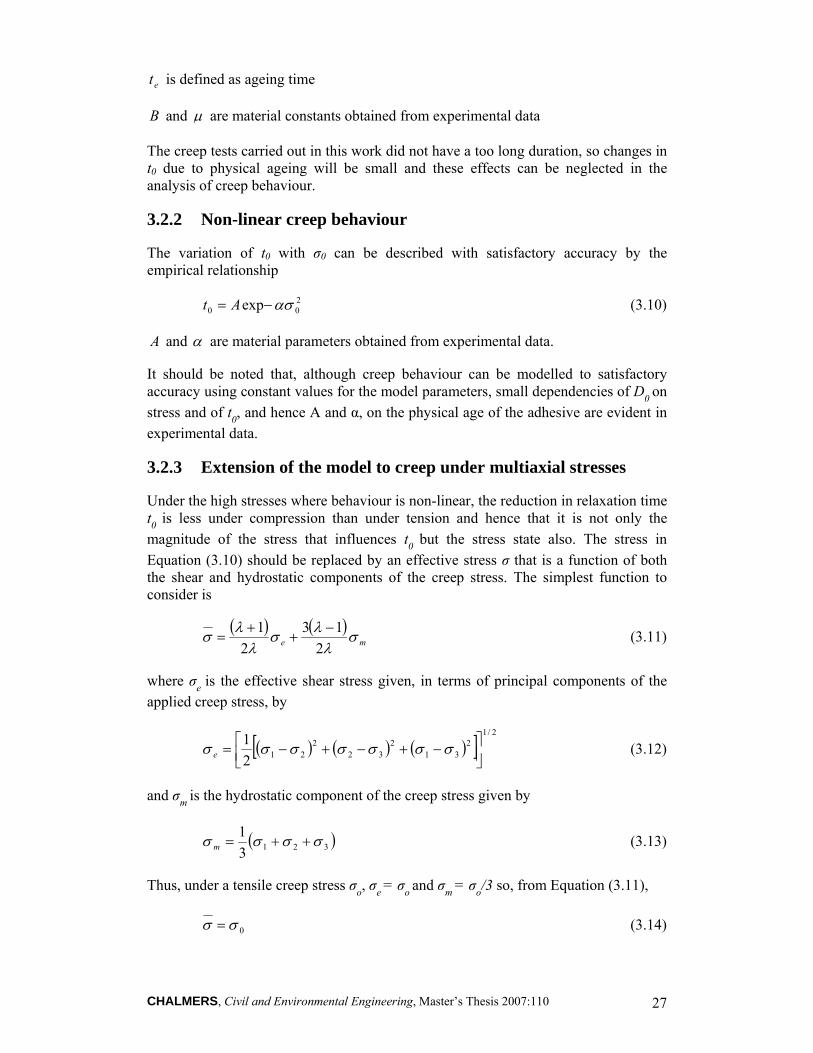
3.2.2 Non-linear creep behaviour
The variation of t0 with σ0 can be described with satisfactory accuracy by the empirical relationship
200 exp ασ−= At (3.10)
A and α are material parameters obtained from experimental data.
It should be noted that, although creep behaviour can be modelled to satisfactory accuracy using constant values for the model parameters, small dependencies of D0 on stress and of t0, and hence A and α, on the physical age of the adhesive are evident in experimental data.
3.2.3 Extension of the model to creep under multiaxial stresses
Under the high stresses where behaviour is non-linear, the reduction in relaxation time t0 is less under compression than under tension and hence that it is not only the magnitude of the stress that influences t0 but the stress state also. The stress in Equation (3.10) should be replaced by an effective stress σ that is a function of both the shear and hydrostatic components of the creep stress. The simplest function to consider is
( ) ( )me σ
λλσ
λλσ
213
21 −
++
= (3.11)
where σe is the effective shear stress given, in terms of principal components of the applied creep stress, by
( ) ( ) ( )[ ]2/1
231
232
2212
1⎥⎦⎤
⎢⎣⎡ −+−+−= σσσσσσσ e (3.12)
and σm is the hydrostatic component of the creep stress given by
( )32131 σσσσ ++=m (3.13)
Thus, under a tensile creep stress σo, σe = σo and σm = σo/3 so, from Equation (3.11),
0σσ = (3.14)
CHALMERS, Civil and Environmental Engineering, Master’s Thesis 2007:110 28
Under a compressive creep stress σc, σe = σc and σm = -σc/3, so
cσλ
σ 1= (1.13)
3.2.4 Effect of different parameters
3.2.4.1 Stress Effect
The creep spectrum is stress-dependent when the stress level is increased from linear to nonlinear viscoelastic region. In the linear viscoelastic region, the creep strain is a linear function of stress, which means the creep compliance is independent of applied stress levels. Polymeric materials generally exhibit linear viscoelastic behaviour at low stresses such that the corresponding strain is at 0.5% or less, Feng (2004). As the stress level is increased, deviation from the linearity can be found, indicating a nonlinear behaviour, which causes difficulty to construct a master curve based on Time-Temperature Superposition principle [see section xxx]. Additionally, the time at which the curves start to become nonlinear decreases with the increasing stress levels.
3.2.4.2 Temperature Effect
It is well known that a change of the temperature has a dramatic effect on the mechanical properties of polymers because a higher molecular mobility is expected at elevated temperatures. Glass transition temperature (Tg), only observed in the polymeric materials, indicates the structural change between glassy and rubbery state. Tg is regarded as a critical reference temperature for assessing mechanical performance of polymers. Tg – 20°C is usually considered as a limiting use temperature for most applications since a significant loss of mechanical performance may occur at this temperature level, Feng (2004). Previous findings have shown that the tensile modulus of epoxy resin can drop drastically when temperatures approach Tg. These results suggest that the viscoelastic responses of materials essentially become highly nonlinear when the temperature is close to Tg and the service temperature of epoxy adhesives should be strictly limited by this transition temperature.
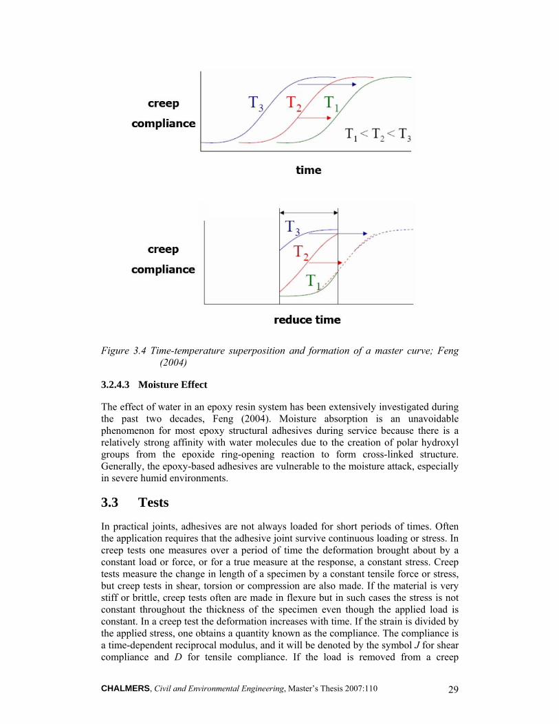
Time-Temperature Superposition
The creep behaviour occurs by molecular diffusional motions which become more rapid when the test temperature is increased. The well-established time-temperature superposition principle states quantitatively that for viscoelastic materials, time and temperature are equivalent to the extent that data at one temperature can be superimposed on data at another temperature by shifting the curves along the time scale as shown in Figure 3.4.
CHALMERS, Civil and Environmental Engineering, Master’s Thesis 2007:110 29
Figure 3.4 Time-temperature superposition and formation of a master curve; Feng (2004)
3.2.4.3 Moisture Effect
The effect of water in an epoxy resin system has been extensively investigated during the past two decades, Feng (2004). Moisture absorption is an unavoidable phenomenon for most epoxy structural adhesives during service because there is a relatively strong affinity with water molecules due to the creation of polar hydroxyl groups from the epoxide ring-opening reaction to form cross-linked structure. Generally, the epoxy-based adhesives are vulnerable to the moisture attack, especially in severe humid environments.
3.3 Tests
In practical joints, adhesives are not always loaded for short periods of times. Often the application requires that the adhesive joint survive continuous loading or stress. In creep tests one measures over a period of time the deformation brought about by a constant load or force, or for a true measure at the response, a constant stress. Creep tests measure the change in length of a specimen by a constant tensile force or stress, but creep tests in shear, torsion or compression are also made. If the material is very stiff or brittle, creep tests often are made in flexure but in such cases the stress is not constant throughout the thickness of the specimen even though the applied load is constant. In a creep test the deformation increases with time. If the strain is divided by the applied stress, one obtains a quantity known as the compliance. The compliance is a time-dependent reciprocal modulus, and it will be denoted by the symbol J for shear compliance and D for tensile compliance. If the load is removed from a creep
CHALMERS, Civil and Environmental Engineering, Master’s Thesis 2007:110 30
specimen after some time, there is a tendency for the specimen to return to its original length or shape. A recovery curve is thus obtained if the deformation is plotted as a function of time after removal of the load.
There are no special tests for creep in the bulk adhesives available in the standards, though the ones for plastics can be used. Some of them are outlined below:
• D2990-01. Standard Test Methods for Tensile, Compressive, and Flexural creep and creep-Rupture of plastics. These test methods cover the determination of tensile and compressive creep and creep-rupture of plastics under specified environmental conditions. For measurements of creep-rupture, tension is the preferred stress mode because for some ductile plastics rupture does not occur in flexure or compression.
• ISO 899-1. Plastics -- Determination of creep behaviour -- Part 1: Tensile creep. This standard specifies a method for determining the tensile creep of plastics in the form of standard test specimens under specified conditions such as those of pre-treatment, temperature and humidity.
The resistance to creep of any joint system can be assessed by either using standard test piece geometries, such as the lap-shear or the T-peel specimens. Some Standard test methods are given below, including the assessment of environmental effects on creep-rupture.
• ASTM D1780-99. Standard Practice for Conducting Creep Tests of Metal-to-Metal Adhesives. This practice covers the determination of the amount of creep of metal-to-metal adhesive bonds due to the combined effects of temperature, tensile shear stress, and time.
• ASTM D2293-96(2002). Standard Test Method for Creep Properties of Adhesives in Shear by Compression Loading (Metal-to-Metal). This test method covers the determination of the creep properties of adhesives for bonding metals when tested on a standard specimen and subjected to certain conditions of temperature and compressive stress in a spring-loaded testing apparatus.
• ASTM D2294-96(2002). Standard Test Method for Creep Properties of Adhesives in Shear by Tensile Loading (Metal-to-Metal). This standard defines a test for creep properties of adhesives utilizing a spring-loaded apparatus to maintain constant stress. With this apparatus once loaded, the elongation of the lap shear specimen is measured by observing the separation of fine razor scratches across its polished edges through a microscope.
• ASTM D2919-01. Standard Test Method for Determining Durability of Adhesive Joints Stressed in Shear by Tension Loading (lap shear). This test method provides data for assessing the durability of adhesive lap-shear joints while stressed in contact with air, air in equilibrium with certain solutions, water, aqueous solutions, or other environments at various temperatures.
• ISO 15109:1998. Determination of the time to failure of bonded joints under static loads. This International Standard describes a procedure for the determination of the time to failure of a bonded joint, using a specimen which
CHALMERS, Civil and Environmental Engineering, Master’s Thesis 2007:110 31
is statically loaded under specified conditions. This method can only be used for comparing adhesives, and the results cannot be used for design.
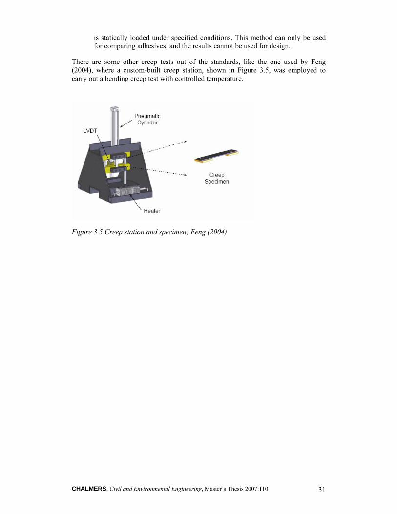
There are some other creep tests out of the standards, like the one used by Feng (2004), where a custom-built creep station, shown in Figure 3.5, was employed to carry out a bending creep test with controlled temperature.
Figure 3.5 Creep station and specimen; Feng (2004)

CHALMERS, Civil and Environmental Engineering, Master’s Thesis 2007:110 32

CHALMERS, Civil and Environmental Engineering, Master’s Thesis 2007:110 33
4 Material Testing
4.1 Creep test
Specimens for creep tests had dogbone shape, they were 225 mm long and had a thickness of 2 mm, Gommersall et al (1996); see Figure 4.1. Specimens were cast in special aluminium moulds which consisted of 6 aluminium frames with a Teflon plate at the bottom, see Figure 4.2
Figure 4.1 Dimensions of creep test epoxy specimen (all dimensions in mm)
Figure 4.2 Casting mould
CHALMERS, Civil and Environmental Engineering, Master’s Thesis 2007:110 34
4.1.1 Manufacturing of test specimens
The specimens were manufactured in the Laboratory of Civil Engineering Department at Chalmers University according to the supplier’s specification. Two different commercial adhesives were tested: Epoxy A and Epoxy B. Before the specimens were cast, the moulds were cleaned and their surfaces were sprayed with CRC “Dry Lube” Teflon spray.
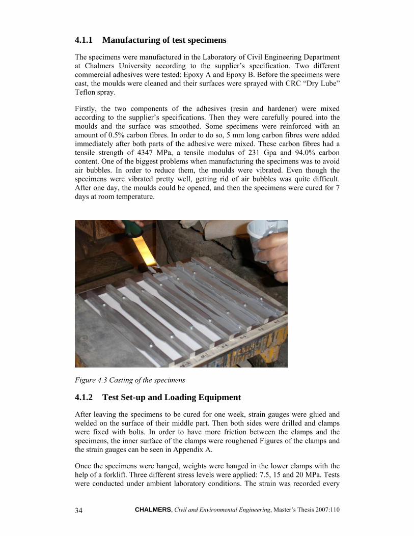
Firstly, the two components of the adhesives (resin and hardener) were mixed according to the supplier’s specifications. Then they were carefully poured into the moulds and the surface was smoothed. Some specimens were reinforced with an amount of 0.5% carbon fibres. In order to do so, 5 mm long carbon fibres were added immediately after both parts of the adhesive were mixed. These carbon fibres had a tensile strength of 4347 MPa, a tensile modulus of 231 Gpa and 94.0% carbon content. One of the biggest problems when manufacturing the specimens was to avoid air bubbles. In order to reduce them, the moulds were vibrated. Even though the specimens were vibrated pretty well, getting rid of air bubbles was quite difficult. After one day, the moulds could be opened, and then the specimens were cured for 7 days at room temperature.
Figure 4.3 Casting of the specimens
4.1.2 Test Set-up and Loading Equipment
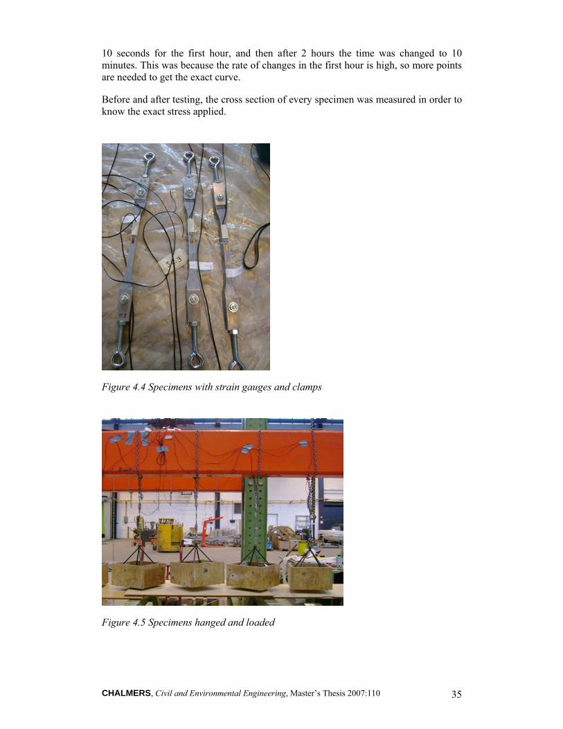
After leaving the specimens to be cured for one week, strain gauges were glued and welded on the surface of their middle part. Then both sides were drilled and clamps were fixed with bolts. In order to have more friction between the clamps and the specimens, the inner surface of the clamps were roughened Figures of the clamps and the strain gauges can be seen in Appendix A.
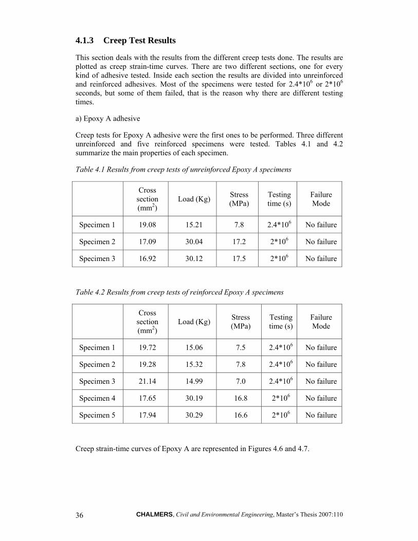
Once the specimens were hanged, weights were hanged in the lower clamps with the help of a forklift. Three different stress levels were applied: 7.5, 15 and 20 MPa. Tests were conducted under ambient laboratory conditions. The strain was recorded every
CHALMERS, Civil and Environmental Engineering, Master’s Thesis 2007:110 35
10 seconds for the first hour, and then after 2 hours the time was changed to 10 minutes. This was because the rate of changes in the first hour is high, so more points are needed to get the exact curve.
Before and after testing, the cross section of every specimen was measured in order to know the exact stress applied.
Figure 4.4 Specimens with strain gauges and clamps
Figure 4.5 Specimens hanged and loaded
CHALMERS, Civil and Environmental Engineering, Master’s Thesis 2007:110 36
4.1.3 Creep Test Results
This section deals with the results from the different creep tests done. The results are plotted as creep strain-time curves. There are two different sections, one for every kind of adhesive tested. Inside each section the results are divided into unreinforced and reinforced adhesives. Most of the specimens were tested for 2.4*106 or 2*106
seconds, but some of them failed, that is the reason why there are different testing times.
a) Epoxy A adhesive
Creep tests for Epoxy A adhesive were the first ones to be performed. Three different unreinforced and five reinforced specimens were tested. Tables 4.1 and 4.2 summarize the main properties of each specimen.
Table 4.1 Results from creep tests of unreinforced Epoxy A specimens
Cross section (mm2)
Load (Kg) Stress (MPa)
Testing time (s)
Failure Mode
Specimen 1 19.08 15.21 7.8 2.4*106 No failure
Specimen 2 17.09 30.04 17.2 2*106 No failure
Specimen 3 16.92 30.12 17.5 2*106 No failure
Table 4.2 Results from creep tests of reinforced Epoxy A specimens
Cross section (mm2)
Load (Kg) Stress (MPa)
Testing time (s)
Failure Mode
Specimen 1 19.72 15.06 7.5 2.4*106 No failure
Specimen 2 19.28 15.32 7.8 2.4*106 No failure
Specimen 3 21.14 14.99 7.0 2.4*106 No failure
Specimen 4 17.65 30.19 16.8 2*106 No failure
Specimen 5 17.94 30.29 16.6 2*106 No failure
Creep strain-time curves of Epoxy A are represented in Figures 4.6 and 4.7.
CHALMERS, Civil and Environmental Engineering, Master’s Thesis 2007:110 37
0
0,2
0,4
0,6
0,8
1
1,2
1,4
0 500000 1000000 1500000 2000000 2500000 3000000
Time (s)
Cre
ep s
train
Specimen 1 - 7.8 MPa
Specimen 2 - 17.2 MPa
Specimen 3 - 17.5 MPa
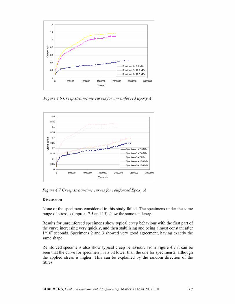
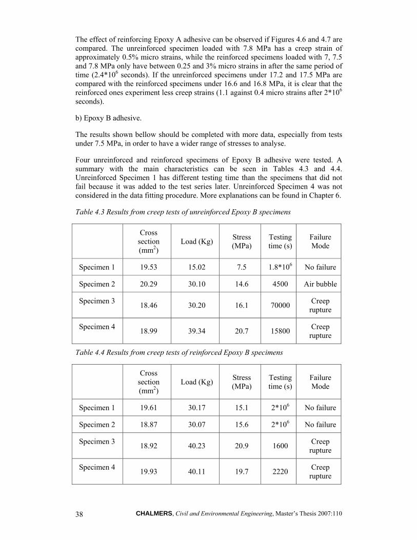
Figure 4.6 Creep strain-time curves for unreinforced Epoxy A
0
0,05
0,1
0,15
0,2
0,25
0,3
0,35
0,4
0,45
0,5
0 500000 1000000 1500000 2000000 2500000 3000000
Time (s)
Cre
ep s
trai
n
Specimen 1 - 7.5 MPa
Specimen 2 - 7.8 MPa
Specimen 3 - 7 MPa
Specimen 4 - 16.8 MPa
Specimen 5 - 16.6 MPa
Figure 4.7 Creep strain-time curves for reinforced Epoxy A
Discussion
None of the specimens considered in this study failed. The specimens under the same range of stresses (approx. 7.5 and 15) show the same tendency.
Results for unreinforced specimens show typical creep behaviour with the first part of the curve increasing very quickly, and then stabilising and being almost constant after 1*106 seconds. Specimens 2 and 3 showed very good agreement, having exactly the same shape.
Reinforced specimens also show typical creep behaviour. From Figure 4.7 it can be seen that the curve for specimen 1 is a bit lower than the one for specimen 2, although the applied stress is higher. This can be explained by the random direction of the fibres.
CHALMERS, Civil and Environmental Engineering, Master’s Thesis 2007:110 38
The effect of reinforcing Epoxy A adhesive can be observed if Figures 4.6 and 4.7 are compared. The unreinforced specimen loaded with 7.8 MPa has a creep strain of approximately 0.5% micro strains, while the reinforced specimens loaded with 7, 7.5 and 7.8 MPa only have between 0.25 and 3% micro strains in after the same period of time (2.4*106 seconds). If the unreinforced specimens under 17.2 and 17.5 MPa are compared with the reinforced specimens under 16.6 and 16.8 MPa, it is clear that the reinforced ones experiment less creep strains (1.1 against 0.4 micro strains after 2*106 seconds).
b) Epoxy B adhesive.
The results shown bellow should be completed with more data, especially from tests under 7.5 MPa, in order to have a wider range of stresses to analyse.
Four unreinforced and reinforced specimens of Epoxy B adhesive were tested. A summary with the main characteristics can be seen in Tables 4.3 and 4.4. Unreinforced Specimen 1 has different testing time than the specimens that did not fail because it was added to the test series later. Unreinforced Specimen 4 was not considered in the data fitting procedure. More explanations can be found in Chapter 6.
Table 4.3 Results from creep tests of unreinforced Epoxy B specimens
Cross section (mm2)
Load (Kg) Stress (MPa)
Testing time (s)
Failure Mode
Specimen 1 19.53 15.02 7.5 1.8*106 No failure
Specimen 2 20.29 30.10 14.6 4500 Air bubble
Specimen 3 18.46 30.20 16.1 70000 Creep rupture
Specimen 4 18.99 39.34 20.7 15800 Creep rupture
Table 4.4 Results from creep tests of reinforced Epoxy B specimens
Cross section (mm2)
Load (Kg) Stress (MPa)
Testing time (s)
Failure Mode
Specimen 1 19.61 30.17 15.1 2*106 No failure
Specimen 2 18.87 30.07 15.6 2*106 No failure
Specimen 3 18.92 40.23 20.9 1600 Creep rupture
Specimen 4 19.93 40.11 19.7 2220 Creep rupture
CHALMERS, Civil and Environmental Engineering, Master’s Thesis 2007:110 39
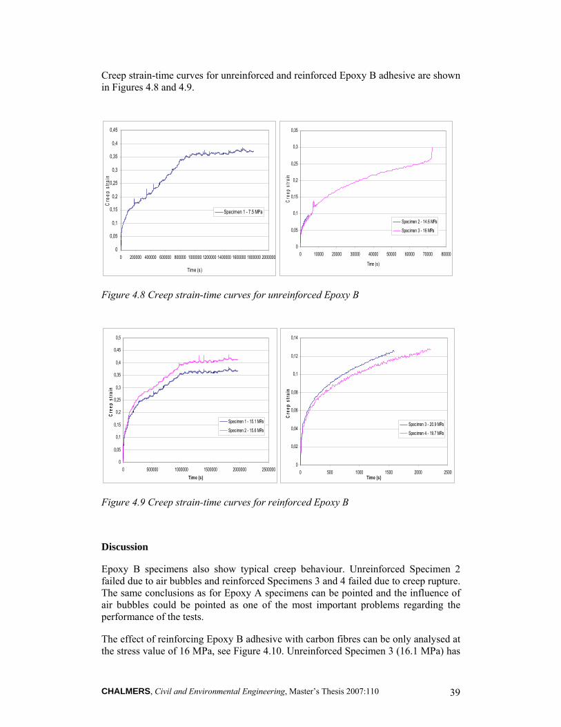
Creep strain-time curves for unreinforced and reinforced Epoxy B adhesive are shown in Figures 4.8 and 4.9.
0
0,05
0,1
0,15
0,2
0,25
0,3
0,35
0,4
0,45
0 200000 400000 600000 800000 1000000 1200000 1400000 1600000 1800000 2000000
Time (s)
Cre
ep s
train
Specimen 1 - 7.5 MPa
0
0,05
0,1
0,15
0,2
0,25
0,3
0,35
0 10000 20000 30000 40000 50000 60000 70000 80000
Time (s)
Cre
ep s
train
Specimen 2 - 14.6 MPa
Specimen 3 - 16 MPa
Figure 4.8 Creep strain-time curves for unreinforced Epoxy B
0
0,05
0,1
0,15
0,2
0,25
0,3
0,35
0,4
0,45
0,5
0 500000 1000000 1500000 2000000 2500000Time (s)
Cre
ep s
trai
n
Specimen 1 - 15.1 MPa
Specimen 2 - 15.6 MPa
0
0,02
0,04
0,06
0,08
0,1
0,12
0,14
0 500 1000 1500 2000 2500Time (s)
Cre
ep s
trai
n
Specimen 3 - 20.9 MPa
Specimen 4 - 19.7 MPa
Figure 4.9 Creep strain-time curves for reinforced Epoxy B
Discussion
Epoxy B specimens also show typical creep behaviour. Unreinforced Specimen 2 failed due to air bubbles and reinforced Specimens 3 and 4 failed due to creep rupture. The same conclusions as for Epoxy A specimens can be pointed and the influence of air bubbles could be pointed as one of the most important problems regarding the performance of the tests.
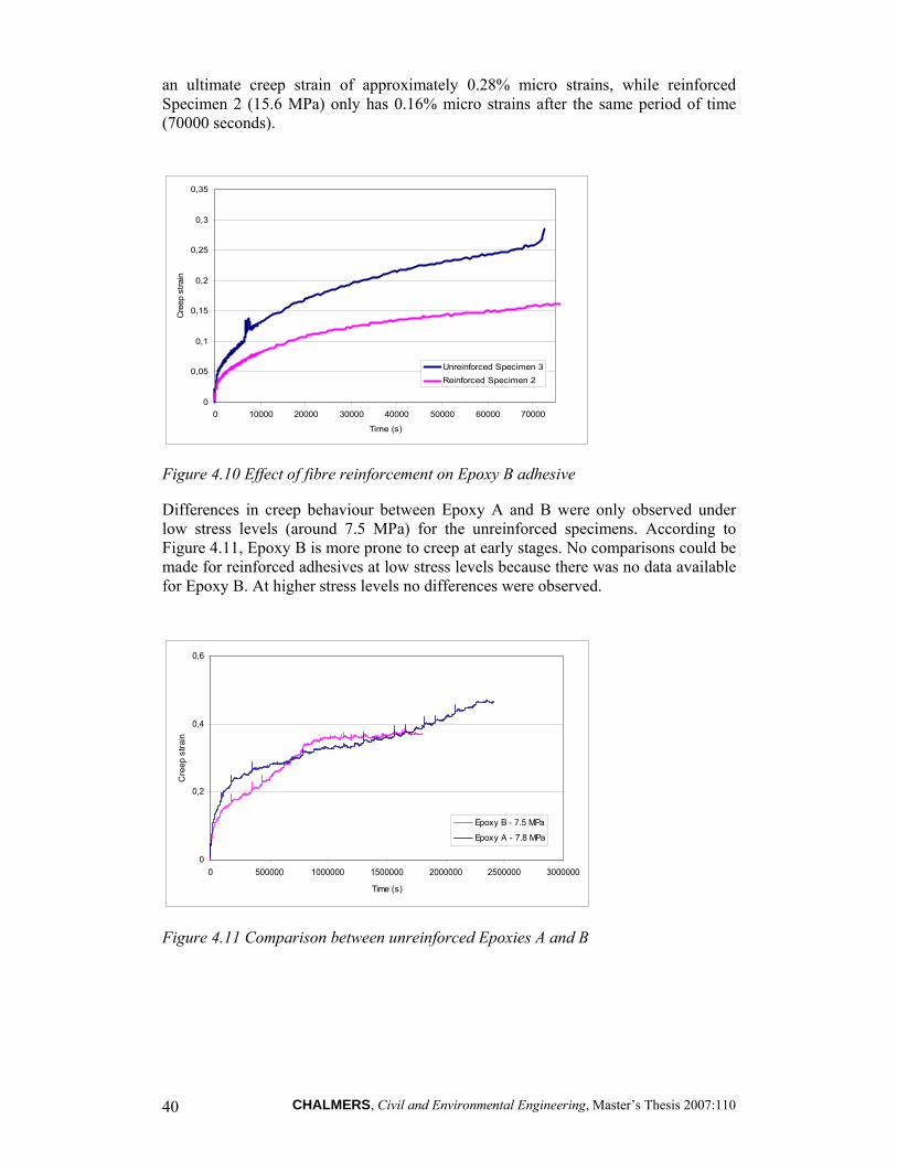
The effect of reinforcing Epoxy B adhesive with carbon fibres can be only analysed at the stress value of 16 MPa, see Figure 4.10. Unreinforced Specimen 3 (16.1 MPa) has
CHALMERS, Civil and Environmental Engineering, Master’s Thesis 2007:110 40
an ultimate creep strain of approximately 0.28% micro strains, while reinforced Specimen 2 (15.6 MPa) only has 0.16% micro strains after the same period of time (70000 seconds).
0
0,05
0,1
0,15
0,2
0,25
0,3
0,35
0 10000 20000 30000 40000 50000 60000 70000
Time (s)
Cre
ep s
train
Unreinforced Specimen 3Reinforced Specimen 2
Figure 4.10 Effect of fibre reinforcement on Epoxy B adhesive
Differences in creep behaviour between Epoxy A and B were only observed under low stress levels (around 7.5 MPa) for the unreinforced specimens. According to Figure 4.11, Epoxy B is more prone to creep at early stages. No comparisons could be made for reinforced adhesives at low stress levels because there was no data available for Epoxy B. At higher stress levels no differences were observed.
0
0,2
0,4
0,6
0 500000 1000000 1500000 2000000 2500000 3000000
Time (s)
Cre
ep s
train
Epoxy B - 7.5 MPa
Epoxy A - 7.8 MPa
Figure 4.11 Comparison between unreinforced Epoxies A and B
CHALMERS, Civil and Environmental Engineering, Master’s Thesis 2007:110 41
4.2 Tensile Test
Tensile tests were also performed in the two adhesives studied in this Master Thesis. According to the manufacturer’s data, Epoxy A adhesive had an ultimate tensile strength of 30 MPa and a Young’s modulus of 4.5 GPa. These values were provided by the manufacturer. On the other hand, according to the Master Thesis titled “Experimental Study of Steel-CFRP Composite Elements” carried out at Chalmers University (Ingles, Mendoza 2004), Epoxy B adhesive is expected to have a Young’s modulus of 24 MPa and an ultimate tensile strength of 6 GPa. All the test procedure and the results obtained are explained in this chapter.
4.2.1 Test Specimen
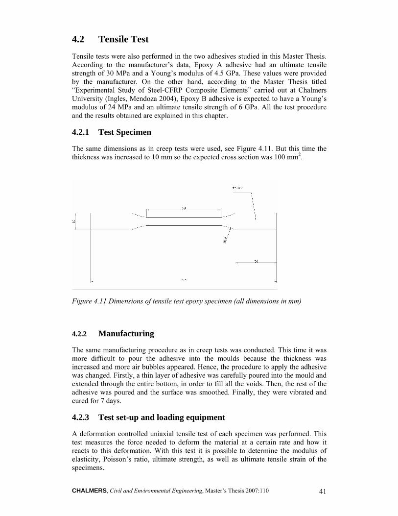
The same dimensions as in creep tests were used, see Figure 4.11. But this time the thickness was increased to 10 mm so the expected cross section was 100 mm2.
Figure 4.11 Dimensions of tensile test epoxy specimen (all dimensions in mm)
4.2.2 Manufacturing
The same manufacturing procedure as in creep tests was conducted. This time it was more difficult to pour the adhesive into the moulds because the thickness was increased and more air bubbles appeared. Hence, the procedure to apply the adhesive was changed. Firstly, a thin layer of adhesive was carefully poured into the mould and extended through the entire bottom, in order to fill all the voids. Then, the rest of the adhesive was poured and the surface was smoothed. Finally, they were vibrated and cured for 7 days.
4.2.3 Test set-up and loading equipment
A deformation controlled uniaxial tensile test of each specimen was performed. This test measures the force needed to deform the material at a certain rate and how it reacts to this deformation. With this test it is possible to determine the modulus of elasticity, Poisson’s ratio, ultimate strength, as well as ultimate tensile strain of the specimens.
CHALMERS, Civil and Environmental Engineering, Master’s Thesis 2007:110 42
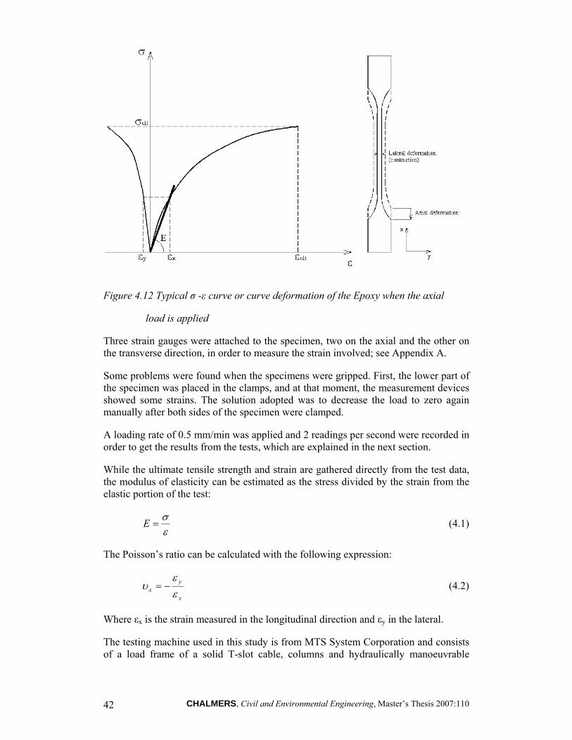
Figure 4.12 Typical σ -ε curve or curve deformation of the Epoxy when the axial
load is applied
Three strain gauges were attached to the specimen, two on the axial and the other on the transverse direction, in order to measure the strain involved; see Appendix A.
Some problems were found when the specimens were gripped. First, the lower part of the specimen was placed in the clamps, and at that moment, the measurement devices showed some strains. The solution adopted was to decrease the load to zero again manually after both sides of the specimen were clamped.
A loading rate of 0.5 mm/min was applied and 2 readings per second were recorded in order to get the results from the tests, which are explained in the next section.
While the ultimate tensile strength and strain are gathered directly from the test data, the modulus of elasticity can be estimated as the stress divided by the strain from the elastic portion of the test:
εσ
=E (4.1)
The Poisson’s ratio can be calculated with the following expression:
x
yx ε
ευ −= (4.2)
Where εx is the strain measured in the longitudinal direction and εy in the lateral.
The testing machine used in this study is from MTS System Corporation and consists of a load frame of a solid T-slot cable, columns and hydraulically manoeuvrable
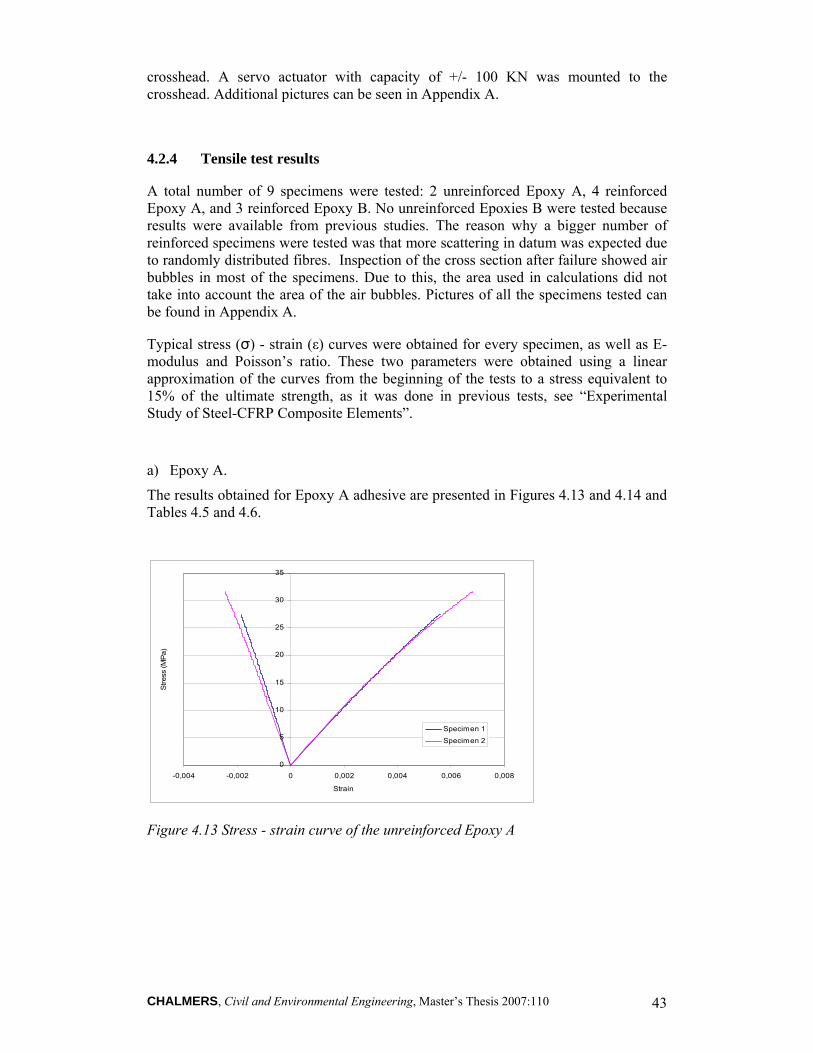
CHALMERS, Civil and Environmental Engineering, Master’s Thesis 2007:110 43
crosshead. A servo actuator with capacity of +/- 100 KN was mounted to the crosshead. Additional pictures can be seen in Appendix A.
4.2.4 Tensile test results
A total number of 9 specimens were tested: 2 unreinforced Epoxy A, 4 reinforced Epoxy A, and 3 reinforced Epoxy B. No unreinforced Epoxies B were tested because results were available from previous studies. The reason why a bigger number of reinforced specimens were tested was that more scattering in datum was expected due to randomly distributed fibres. Inspection of the cross section after failure showed air bubbles in most of the specimens. Due to this, the area used in calculations did not take into account the area of the air bubbles. Pictures of all the specimens tested can be found in Appendix A.
Typical stress (σ) - strain (ε) curves were obtained for every specimen, as well as E-modulus and Poisson’s ratio. These two parameters were obtained using a linear approximation of the curves from the beginning of the tests to a stress equivalent to 15% of the ultimate strength, as it was done in previous tests, see “Experimental Study of Steel-CFRP Composite Elements”.
a) Epoxy A.
The results obtained for Epoxy A adhesive are presented in Figures 4.13 and 4.14 and Tables 4.5 and 4.6.
0
5
10
15
20
25
30
35
-0,004 -0,002 0 0,002 0,004 0,006 0,008
Strain
Stre
ss (M
Pa)
Specimen 1
Specimen 2
Figure 4.13 Stress - strain curve of the unreinforced Epoxy A
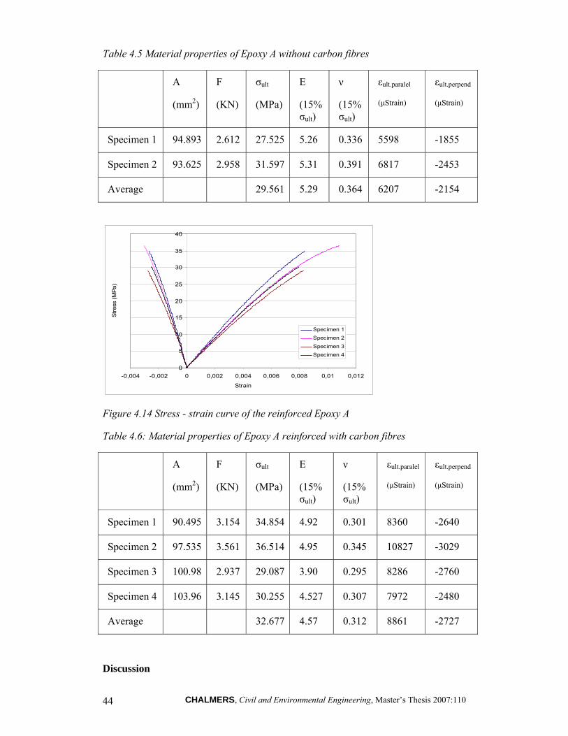
CHALMERS, Civil and Environmental Engineering, Master’s Thesis 2007:110 44
Table 4.5 Material properties of Epoxy A without carbon fibres
A
(mm2)
F
(KN)
σult
(MPa)
E
(15% σult)
ν
(15% σult)
εult.paralel
(μStrain)
εult.perpend
(μStrain)
Specimen 1 94.893 2.612 27.525 5.26 0.336 5598 -1855
Specimen 2 93.625 2.958 31.597 5.31 0.391 6817 -2453
Average 29.561 5.29 0.364 6207 -2154
0
5
10
15
20
25
30
35
40
-0,004 -0,002 0 0,002 0,004 0,006 0,008 0,01 0,012
Strain
Stre
ss (M
Pa)
Specimen 1Specimen 2Specimen 3Specimen 4
Figure 4.14 Stress - strain curve of the reinforced Epoxy A
Table 4.6: Material properties of Epoxy A reinforced with carbon fibres
A
(mm2)
F
(KN)
σult
(MPa)
E
(15% σult)
ν
(15% σult)
εult.paralel
(μStrain)
εult.perpend
(μStrain)
Specimen 1 90.495 3.154 34.854 4.92 0.301 8360 -2640
Specimen 2 97.535 3.561 36.514 4.95 0.345 10827 -3029
Specimen 3 100.98 2.937 29.087 3.90 0.295 8286 -2760
Specimen 4 103.96 3.145 30.255 4.527 0.307 7972 -2480
Average 32.677 4.57 0.312 8861 -2727
Discussion
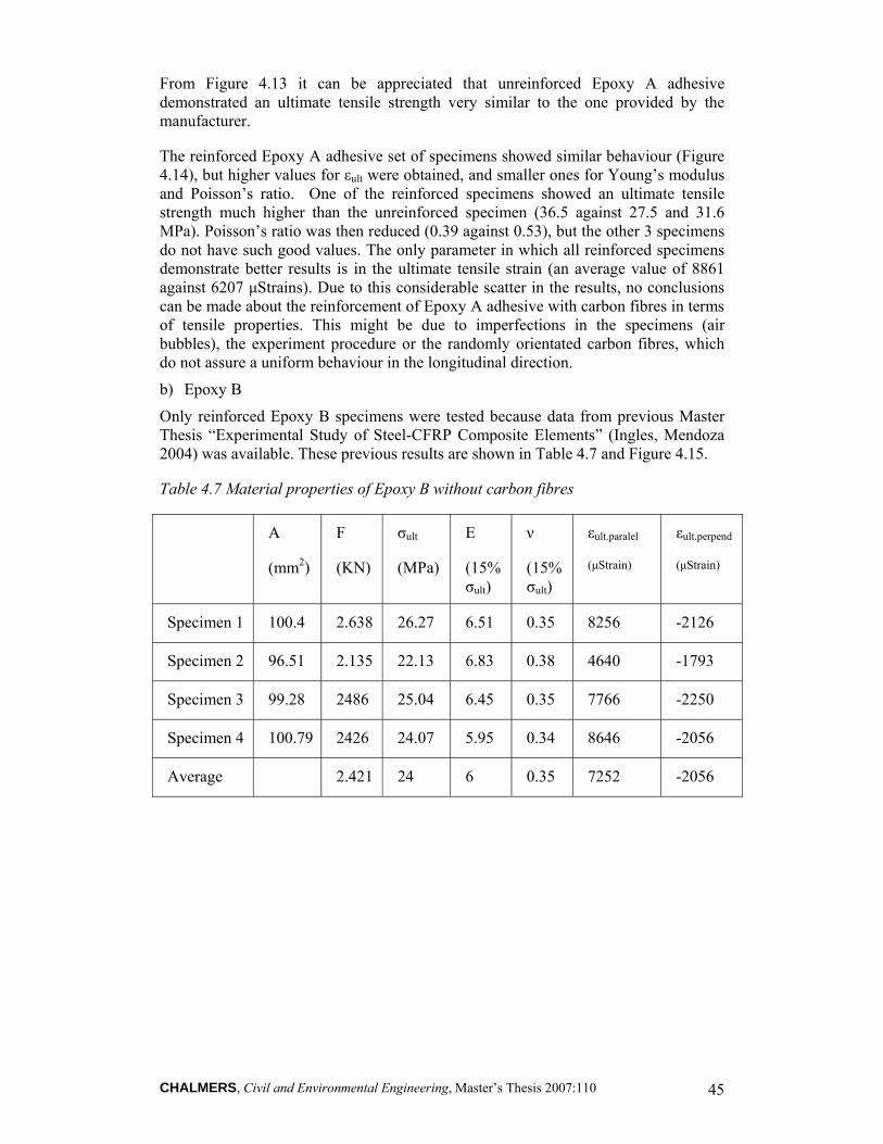
CHALMERS, Civil and Environmental Engineering, Master’s Thesis 2007:110 45
From Figure 4.13 it can be appreciated that unreinforced Epoxy A adhesive demonstrated an ultimate tensile strength very similar to the one provided by the manufacturer.
The reinforced Epoxy A adhesive set of specimens showed similar behaviour (Figure 4.14), but higher values for εult were obtained, and smaller ones for Young’s modulus and Poisson’s ratio. One of the reinforced specimens showed an ultimate tensile strength much higher than the unreinforced specimen (36.5 against 27.5 and 31.6 MPa). Poisson’s ratio was then reduced (0.39 against 0.53), but the other 3 specimens do not have such good values. The only parameter in which all reinforced specimens demonstrate better results is in the ultimate tensile strain (an average value of 8861 against 6207 μStrains). Due to this considerable scatter in the results, no conclusions can be made about the reinforcement of Epoxy A adhesive with carbon fibres in terms of tensile properties. This might be due to imperfections in the specimens (air bubbles), the experiment procedure or the randomly orientated carbon fibres, which do not assure a uniform behaviour in the longitudinal direction.
b) Epoxy B
Only reinforced Epoxy B specimens were tested because data from previous Master Thesis “Experimental Study of Steel-CFRP Composite Elements” (Ingles, Mendoza 2004) was available. These previous results are shown in Table 4.7 and Figure 4.15.
Table 4.7 Material properties of Epoxy B without carbon fibres
A
(mm2)
F
(KN)
σult
(MPa)
E
(15% σult)
ν
(15% σult)
εult.paralel
(μStrain)
εult.perpend
(μStrain)
Specimen 1 100.4 2.638 26.27 6.51 0.35 8256 -2126
Specimen 2 96.51 2.135 22.13 6.83 0.38 4640 -1793
Specimen 3 99.28 2486 25.04 6.45 0.35 7766 -2250
Specimen 4 100.79 2426 24.07 5.95 0.34 8646 -2056
Average 2.421 24 6 0.35 7252 -2056
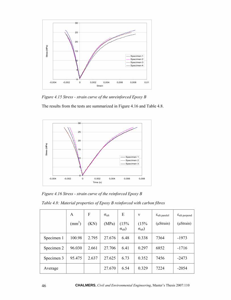
CHALMERS, Civil and Environmental Engineering, Master’s Thesis 2007:110 46
0
5
10
15
20
25
30
-0,004 -0,002 0 0,002 0,004 0,006 0,008 0,01Strain
Stre
ss (M
Pa)
Specimen 1Specimen 2Specimen 3Specimen 4
Figure 4.15 Stress - strain curve of the unreinforced Epoxy B
The results from the tests are summarized in Figure 4.16 and Table 4.8.
0
5
10
15
20
25
30
-0,004 -0,002 0 0,002 0,004 0,006 0,008
Time (s)
Stre
ss (M
Pa)
Specimen 1Specimen 2Specimen 3
Figure 4.16 Stress - strain curve of the reinforced Epoxy B
Table 4.8: Material properties of Epoxy B reinforced with carbon fibres
A
(mm2)
F
(KN)
σult
(MPa)
E
(15% σult)
ν
(15% σult)
εult.paralel
(μStrain)
εult.perpend
(μStrain)
Specimen 1 100.98 2.795 27.676 6.48 0.338 7364 -1973
Specimen 2 96.030 2.661 27.706 6.41 0.297 6852 -1716
Specimen 3 95.475 2.637 27.625 6.73 0.352 7456 -2473
Average 27.670 6.54 0.329 7224 -2054
CHALMERS, Civil and Environmental Engineering, Master’s Thesis 2007:110 47
Discussion
According to the plots, it can be noticed that Epoxy B adhesive shows non-linearity more clearly than Epoxy A. The three specimens show very similar values in terms of ultimate strength, E modulus, Poisson’s ratio and ultimate strain. If they are compared with the previous data available, it can be concluded that there are no differences between the normal adhesive and the reinforced one, so no improvement for ultimate short-term strength is observed by reinforcing Epoxy B adhesive with a 0.5% of carbon fibres.

CHALMERS, Civil and Environmental Engineering, Master’s Thesis 2007:110 48
CHALMERS, Civil and Environmental Engineering, Master’s Thesis 2007:110 49
5 FE Modelling 2D model of the specimens was created and analysed by nonlinear FE analysis method. As a suggestion for further research, a lap shear joint was also modelled using the constants obtained from the experiments.
5.1 Description of the FE model
There is a number of parameters which are needed as inputs in FE-analysis of creep problems. These material parameters were obtained from the experimental data.
The FE model was loaded with constant load at the lower part of the specimen and creep strains were obtained and compared with the experimental results.
The analysis was done using Abaqus 6.6. The model was created with Abaqus/Cae, which provided a consistent interface based on different modules, where each module defined a logical aspect of the modelling process: geometry, material properties, boundary conditions, loads and steps, and mesh. The code generated for one of the specimens is given in Appendix B.
Geometry
The FE model had the same nominal dimensions as the dogbone specimens used in the tests; see Figure 4.11 in Chapter 4.
Element type
In general, the state of stress in a point can be characterized by six independent normal and shear stress components. However due to the complexity of analyzing problems in three dimensions, it is in some cases possible to reduce the analysis to a single plane by assuming a state of plane stress. By assuming that this small principal stress is zero, the three dimensional stress state can be reduced to two dimensions. Since the remaining two principal stresses lie in a plane, these simplified 2D problems are called plane stress problems.
The model was not subjected to out of plane bending, so plane stress elements were sufficient to predict the creep behaviour. 8 node biquadratic elements with reduced integration (CPS8R) were used. Reduced-integration elements use one fewer integration point in each direction than the fully integrated elements. One of the main advantages of reduced integration is that the reduced number of integration points decreases CPU time and storage requirements.
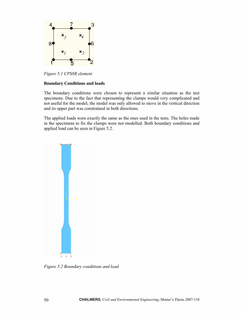
CHALMERS, Civil and Environmental Engineering, Master’s Thesis 2007:110 50
Figure 5.1 CPS8R element
Boundary Conditions and loads
The boundary conditions were chosen to represent a similar situation as the test specimens. Due to the fact that representing the clamps would very complicated and not useful for the model, the model was only allowed to move in the vertical direction and its upper part was constrained in both directions.
The applied loads were exactly the same as the ones used in the tests. The holes made in the specimens to fix the clamps were not modelled. Both boundary conditions and applied load can be seen in Figure 5.2.
Figure 5.2 Boundary conditions and load
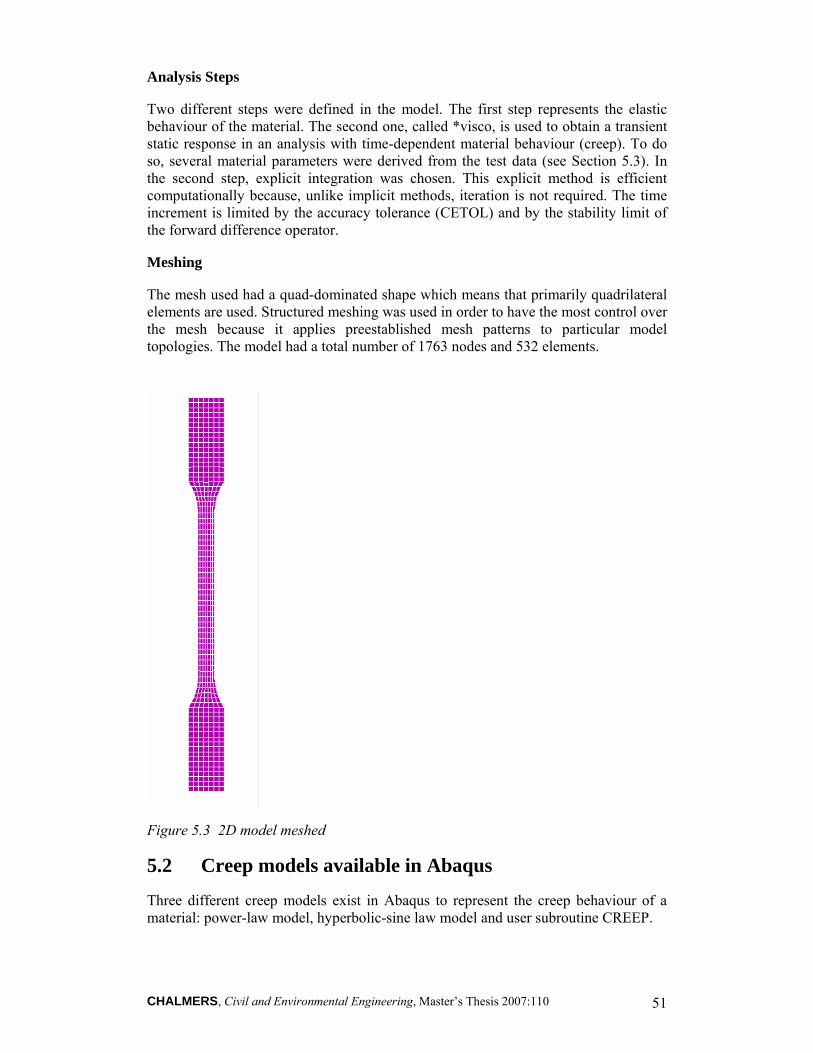
CHALMERS, Civil and Environmental Engineering, Master’s Thesis 2007:110 51
Analysis Steps
Two different steps were defined in the model. The first step represents the elastic behaviour of the material. The second one, called *visco, is used to obtain a transient static response in an analysis with time-dependent material behaviour (creep). To do so, several material parameters were derived from the test data (see Section 5.3). In the second step, explicit integration was chosen. This explicit method is efficient computationally because, unlike implicit methods, iteration is not required. The time increment is limited by the accuracy tolerance (CETOL) and by the stability limit of the forward difference operator.
Meshing
The mesh used had a quad-dominated shape which means that primarily quadrilateral elements are used. Structured meshing was used in order to have the most control over the mesh because it applies preestablished mesh patterns to particular model topologies. The model had a total number of 1763 nodes and 532 elements.
Figure 5.3 2D model meshed
5.2 Creep models available in Abaqus
Three different creep models exist in Abaqus to represent the creep behaviour of a material: power-law model, hyperbolic-sine law model and user subroutine CREEP.
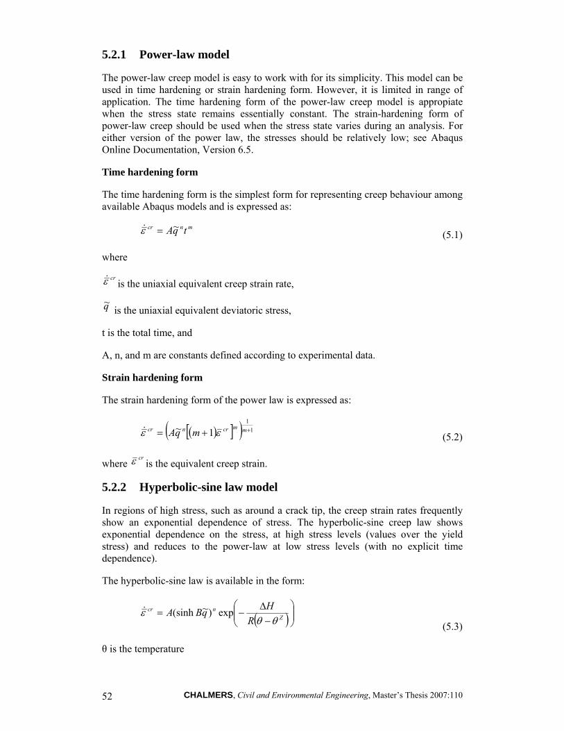
CHALMERS, Civil and Environmental Engineering, Master’s Thesis 2007:110 52
5.2.1 Power-law model
The power-law creep model is easy to work with for its simplicity. This model can be used in time hardening or strain hardening form. However, it is limited in range of application. The time hardening form of the power-law creep model is appropiate when the stress state remains essentially constant. The strain-hardening form of power-law creep should be used when the stress state varies during an analysis. For either version of the power law, the stresses should be relatively low; see Abaqus Online Documentation, Version 6.5.
Time hardening form
The time hardening form is the simplest form for representing creep behaviour among available Abaqus models and is expressed as:
mncr tqA~=ε& (5.1)
where
crε& is the uniaxial equivalent creep strain rate,
q~ is the uniaxial equivalent deviatoric stress,
t is the total time, and
A, n, and m are constants defined according to experimental data.
Strain hardening form
The strain hardening form of the power law is expressed as:
( )[ ]( ) 11
1~ ++= mmcrncr mqA εε& (5.2)
where crε is the equivalent creep strain.
5.2.2 Hyperbolic-sine law model
In regions of high stress, such as around a crack tip, the creep strain rates frequently show an exponential dependence of stress. The hyperbolic-sine creep law shows exponential dependence on the stress, at high stress levels (values over the yield stress) and reduces to the power-law at low stress levels (with no explicit time dependence).
The hyperbolic-sine law is available in the form:
( )⎟⎟⎠⎞
⎜⎜⎝
⎛−Δ
−= Zncr
RHqBAθθ
ε exp)~(sinh&
(5.3)
θ is the temperature
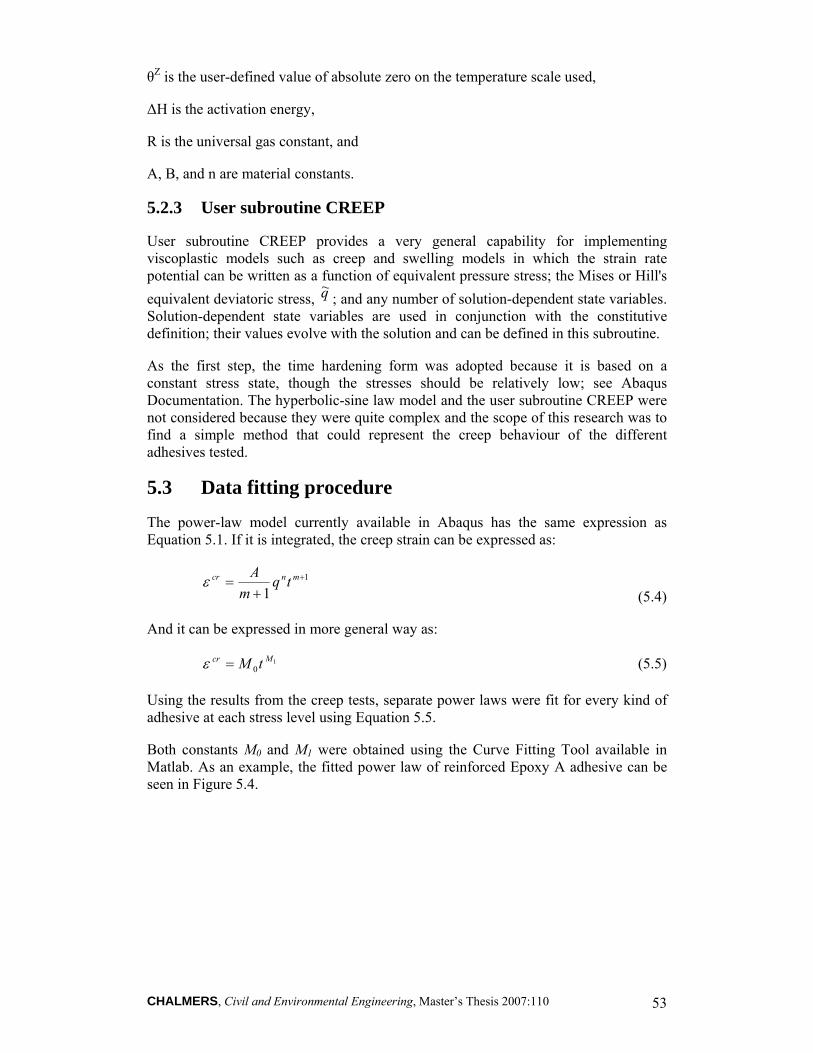
CHALMERS, Civil and Environmental Engineering, Master’s Thesis 2007:110 53
θZ is the user-defined value of absolute zero on the temperature scale used,
ΔH is the activation energy,
R is the universal gas constant, and
A, B, and n are material constants.
5.2.3 User subroutine CREEP
User subroutine CREEP provides a very general capability for implementing viscoplastic models such as creep and swelling models in which the strain rate potential can be written as a function of equivalent pressure stress; the Mises or Hill's equivalent deviatoric stress, q~ ; and any number of solution-dependent state variables. Solution-dependent state variables are used in conjunction with the constitutive definition; their values evolve with the solution and can be defined in this subroutine.
As the first step, the time hardening form was adopted because it is based on a constant stress state, though the stresses should be relatively low; see Abaqus Documentation. The hyperbolic-sine law model and the user subroutine CREEP were not considered because they were quite complex and the scope of this research was to find a simple method that could represent the creep behaviour of the different adhesives tested.
5.3 Data fitting procedure
The power-law model currently available in Abaqus has the same expression as Equation 5.1. If it is integrated, the creep strain can be expressed as:
1
1+
+= mncr tq
mAε
(5.4)
And it can be expressed in more general way as:
10
Mcr tM=ε (5.5)
Using the results from the creep tests, separate power laws were fit for every kind of adhesive at each stress level using Equation 5.5.
Both constants M0 and M1 were obtained using the Curve Fitting Tool available in Matlab. As an example, the fitted power law of reinforced Epoxy A adhesive can be seen in Figure 5.4.
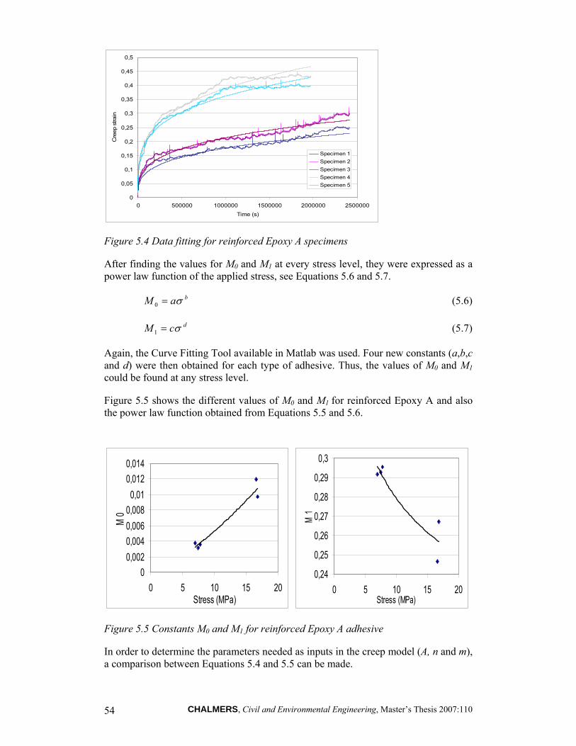
CHALMERS, Civil and Environmental Engineering, Master’s Thesis 2007:110 54
0
0,05
0,1
0,15
0,2
0,25
0,3
0,35
0,4
0,45
0,5
0 500000 1000000 1500000 2000000 2500000Time (s)
Cre
ep s
train
Specimen 1Specimen 2Specimen 3Specimen 4Specimen 5
Figure 5.4 Data fitting for reinforced Epoxy A specimens
After finding the values for M0 and M1 at every stress level, they were expressed as a power law function of the applied stress, see Equations 5.6 and 5.7.
baM σ=0 (5.6)
dcM σ=1 (5.7)
Again, the Curve Fitting Tool available in Matlab was used. Four new constants (a,b,c and d) were then obtained for each type of adhesive. Thus, the values of M0 and M1 could be found at any stress level.
Figure 5.5 shows the different values of M0 and M1 for reinforced Epoxy A and also the power law function obtained from Equations 5.5 and 5.6.
00,0020,0040,0060,008
0,010,0120,014
0 5 10 15 20Stress (MPa)
M0
0,24
0,25
0,26
0,27
0,28
0,29
0,3
0 5 10 15 20Stress (MPa)
M1
Figure 5.5 Constants M0 and M1 for reinforced Epoxy A adhesive
In order to determine the parameters needed as inputs in the creep model (A, n and m), a comparison between Equations 5.4 and 5.5 can be made.
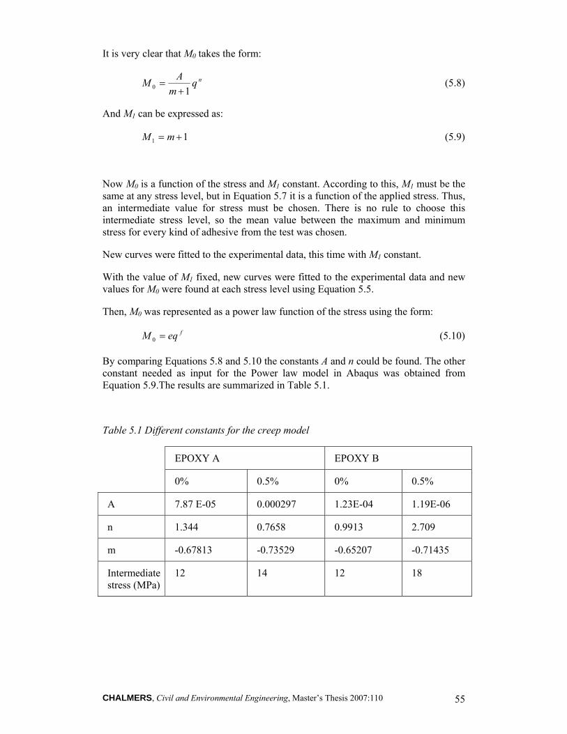
CHALMERS, Civil and Environmental Engineering, Master’s Thesis 2007:110 55
It is very clear that M0 takes the form:
nqm
AM10 +
= (5.8)
And M1 can be expressed as:
11 += mM (5.9)
Now M0 is a function of the stress and M1 constant. According to this, M1 must be the same at any stress level, but in Equation 5.7 it is a function of the applied stress. Thus, an intermediate value for stress must be chosen. There is no rule to choose this intermediate stress level, so the mean value between the maximum and minimum stress for every kind of adhesive from the test was chosen.
New curves were fitted to the experimental data, this time with M1 constant.
With the value of M1 fixed, new curves were fitted to the experimental data and new values for M0 were found at each stress level using Equation 5.5.
Then, M0 was represented as a power law function of the stress using the form:
feqM =0 (5.10)
By comparing Equations 5.8 and 5.10 the constants A and n could be found. The other constant needed as input for the Power law model in Abaqus was obtained from Equation 5.9.The results are summarized in Table 5.1.
Table 5.1 Different constants for the creep model
EPOXY A EPOXY B
0% 0.5% 0% 0.5%
A 7.87 E-05 0.000297 1.23E-04 1.19E-06
n 1.344 0.7658 0.9913 2.709
m -0.67813 -0.73529 -0.65207 -0.71435
Intermediate stress (MPa)
12 14 12 18
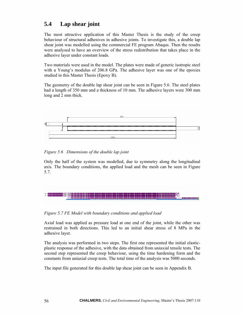
CHALMERS, Civil and Environmental Engineering, Master’s Thesis 2007:110 56
5.4 Lap shear joint
The most attractive application of this Master Thesis is the study of the creep behaviour of structural adhesives in adhesive joints. To investigate this, a double lap shear joint was modelled using the commercial FE program Abaqus. Then the results were analysed to have an overview of the stress redistribution that takes place in the adhesive layer under constant loads.
Two materials were used in the model. The plates were made of generic isotropic steel with a Young’s modulus of 206.8 GPa. The adhesive layer was one of the epoxies studied in this Master Thesis (Epoxy B).
The geometry of the double lap shear joint can be seen in Figure 5.6. The steel plates had a length of 350 mm and a thickness of 10 mm. The adhesive layers were 300 mm long and 2 mm thick.
Figure 5.6 Dimensions of the double lap joint
Only the half of the system was modelled, due to symmetry along the longitudinal axis. The boundary conditions, the applied load and the mesh can be seen in Figure 5.7.
Figure 5.7 FE Model with boundary conditions and applied load
Axial load was applied as pressure load at one end of the joint, while the other was restrained in both directions. This led to an initial shear stress of 8 MPa in the adhesive layer.
The analysis was performed in two steps. The first one represented the initial elastic-plastic response of the adhesive, with the data obtained from uniaxial tensile tests. The second step represented the creep behaviour, using the time hardening form and the constants from uniaxial creep tests. The total time of the analysis was 5000 seconds.
The input file generated for this double lap shear joint can be seen in Appendix B.
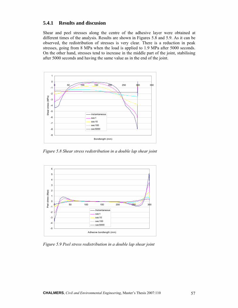
CHALMERS, Civil and Environmental Engineering, Master’s Thesis 2007:110 57
5.4.1 Results and discusion
Shear and peel stresses along the centre of the adhesive layer were obtained at different times of the analysis. Results are shown in Figures 5.8 and 5.9. As it can be observed, the redistribution of stresses is very clear. There is a reduction in peak stresses, going from 8 MPa when the load is applied to 1.9 MPa after 5000 seconds. On the other hand, stresses tend to increase in the middle part of the joint, stabilising after 5000 seconds and having the same value as in the end of the joint.
-9
-8
-7
-6
-5
-4
-3
-2
-1
0
1
0 50 100 150 200 250 300 350
Bondlength (mm)
She
ar s
tress
(MP
a)
instantaneoussec1sec10sec100sec5000
Figure 5.8 Shear stress redistribution in a double lap shear joint
-5
-4
-3
-2
-1
0
1
2
3
4
5
6
0 50 100 150 200 250 300
Adhesive bondlength (mm)
Pee
l stre
ss (M
pa)
Instantaneoussec1sec10sec100sec5000
Figure 5.9 Peel stress redistribution in a double lap shear joint

CHALMERS, Civil and Environmental Engineering, Master’s Thesis 2007:110 58
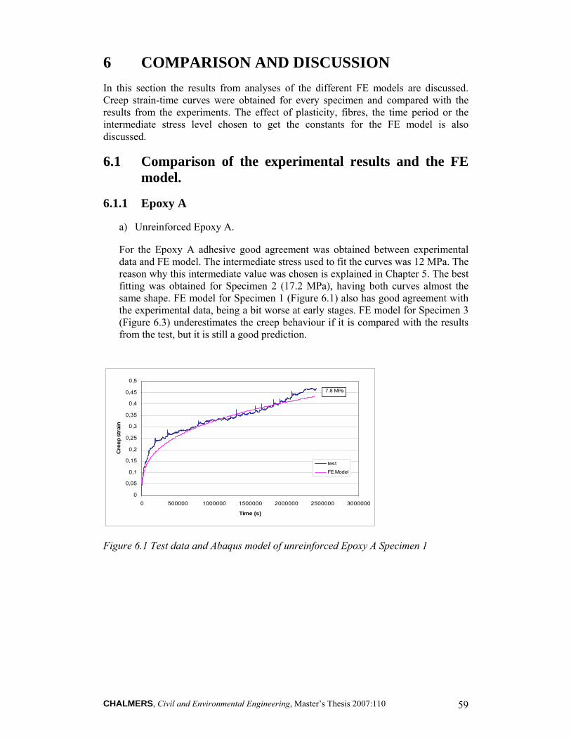
CHALMERS, Civil and Environmental Engineering, Master’s Thesis 2007:110 59
6 COMPARISON AND DISCUSSION In this section the results from analyses of the different FE models are discussed. Creep strain-time curves were obtained for every specimen and compared with the results from the experiments. The effect of plasticity, fibres, the time period or the intermediate stress level chosen to get the constants for the FE model is also discussed.
6.1 Comparison of the experimental results and the FE model.
6.1.1 Epoxy A
a) Unreinforced Epoxy A.
For the Epoxy A adhesive good agreement was obtained between experimental data and FE model. The intermediate stress used to fit the curves was 12 MPa. The reason why this intermediate value was chosen is explained in Chapter 5. The best fitting was obtained for Specimen 2 (17.2 MPa), having both curves almost the same shape. FE model for Specimen 1 (Figure 6.1) also has good agreement with the experimental data, being a bit worse at early stages. FE model for Specimen 3 (Figure 6.3) underestimates the creep behaviour if it is compared with the results from the test, but it is still a good prediction.
0
0,05
0,1
0,15
0,2
0,25
0,3
0,35
0,4
0,45
0,5
0 500000 1000000 1500000 2000000 2500000 3000000
Time (s)
Cre
ep s
trai
n
test
FE Model
7.8 MPa
Figure 6.1 Test data and Abaqus model of unreinforced Epoxy A Specimen 1
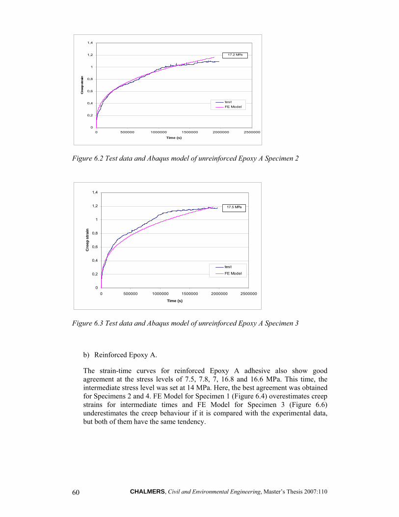
CHALMERS, Civil and Environmental Engineering, Master’s Thesis 2007:110 60
0
0,2
0,4
0,6
0,8
1
1,2
1,4
0 500000 1000000 1500000 2000000 2500000
Time (s)
Cre
ep s
trai
n
testFE Model
17.2 MPa
Figure 6.2 Test data and Abaqus model of unreinforced Epoxy A Specimen 2
0
0,2
0,4
0,6
0,8
1
1,2
1,4
0 500000 1000000 1500000 2000000 2500000
Time (s)
Cre
ep s
trai
n
test
FE Model
17.5 MPa
Figure 6.3 Test data and Abaqus model of unreinforced Epoxy A Specimen 3
b) Reinforced Epoxy A.
The strain-time curves for reinforced Epoxy A adhesive also show good agreement at the stress levels of 7.5, 7.8, 7, 16.8 and 16.6 MPa. This time, the intermediate stress level was set at 14 MPa. Here, the best agreement was obtained for Specimens 2 and 4. FE Model for Specimen 1 (Figure 6.4) overestimates creep strains for intermediate times and FE Model for Specimen 3 (Figure 6.6) underestimates the creep behaviour if it is compared with the experimental data, but both of them have the same tendency.
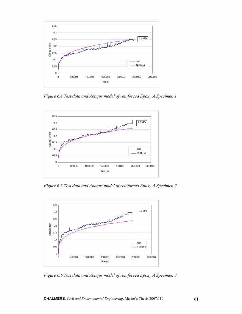
CHALMERS, Civil and Environmental Engineering, Master’s Thesis 2007:110 61
0
0,05
0,1
0,15
0,2
0,25
0,3
0,35
0 500000 1000000 1500000 2000000 2500000 3000000
Time (s)
Cre
ep s
train
testFE Model
7.5 MPa
Figure 6.4 Test data and Abaqus model of reinforced Epoxy A Specimen 1
0
0,05
0,1
0,15
0,2
0,25
0,3
0,35
0 500000 1000000 1500000 2000000 2500000 3000000
Time (s)
Cre
ep s
train
testFE Model
7.8 MPa
Figure 6.5 Test data and Abaqus model of reinforced Epoxy A Specimen 2
0
0,05
0,1
0,15
0,2
0,25
0,3
0,35
0 500000 1000000 1500000 2000000 2500000 3000000
Time (s)
Cre
ep s
train
test
FE Model
7.0 MPa
Figure 6.6 Test data and Abaqus model of reinforced Epoxy A Specimen 3
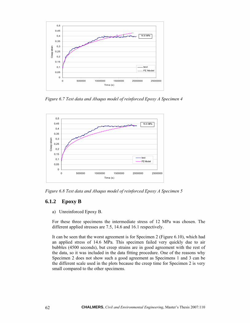
CHALMERS, Civil and Environmental Engineering, Master’s Thesis 2007:110 62
0
0,05
0,1
0,15
0,2
0,25
0,3
0,35
0,4
0,45
0,5
0 500000 1000000 1500000 2000000 2500000
Time (s)
Cre
ep s
train
test
FE Model
16.8 MPa
Figure 6.7 Test data and Abaqus model of reinforced Epoxy A Specimen 4
0
0,05
0,1
0,15
0,2
0,25
0,3
0,35
0,4
0,45
0,5
0 500000 1000000 1500000 2000000 2500000
Time (s)
Cre
ep s
train
testFE Model
16.6 MPa
Figure 6.8 Test data and Abaqus model of reinforced Epoxy A Specimen 5
6.1.2 Epoxy B
a) Unreinforced Epoxy B.
For these three specimens the intermediate stress of 12 MPa was chosen. The different applied stresses are 7.5, 14.6 and 16.1 respectively.
It can be seen that the worst agreement is for Specimen 2 (Figure 6.10), which had an applied stress of 14.6 MPa. This specimen failed very quickly due to air bubbles (4500 seconds), but creep strains are in good agreement with the rest of the data, so it was included in the data fitting procedure. One of the reasons why Specimen 2 does not show such a good agreement as Specimens 1 and 3 can be the different scale used in the plots because the creep time for Specimen 2 is very small compared to the other specimens.
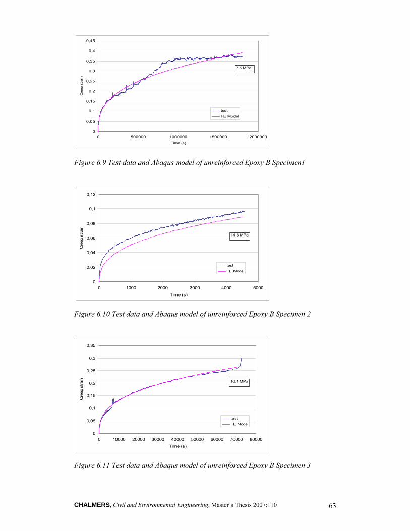
CHALMERS, Civil and Environmental Engineering, Master’s Thesis 2007:110 63
0
0,05
0,1
0,15
0,2
0,25
0,3
0,35
0,4
0,45
0 500000 1000000 1500000 2000000Time (s)
Cre
ep s
train
testFE Model
7.5 MPa
Figure 6.9 Test data and Abaqus model of unreinforced Epoxy B Specimen1
0
0,02
0,04
0,06
0,08
0,1
0,12
0 1000 2000 3000 4000 5000
Time (s)
Cre
ep s
train
testFE Model
14.6 MPa
Figure 6.10 Test data and Abaqus model of unreinforced Epoxy B Specimen 2
0
0,05
0,1
0,15
0,2
0,25
0,3
0,35
0 10000 20000 30000 40000 50000 60000 70000 80000
Time (s)
Cre
ep s
train
testFE Model
16.1 MPa
Figure 6.11 Test data and Abaqus model of unreinforced Epoxy B Specimen 3
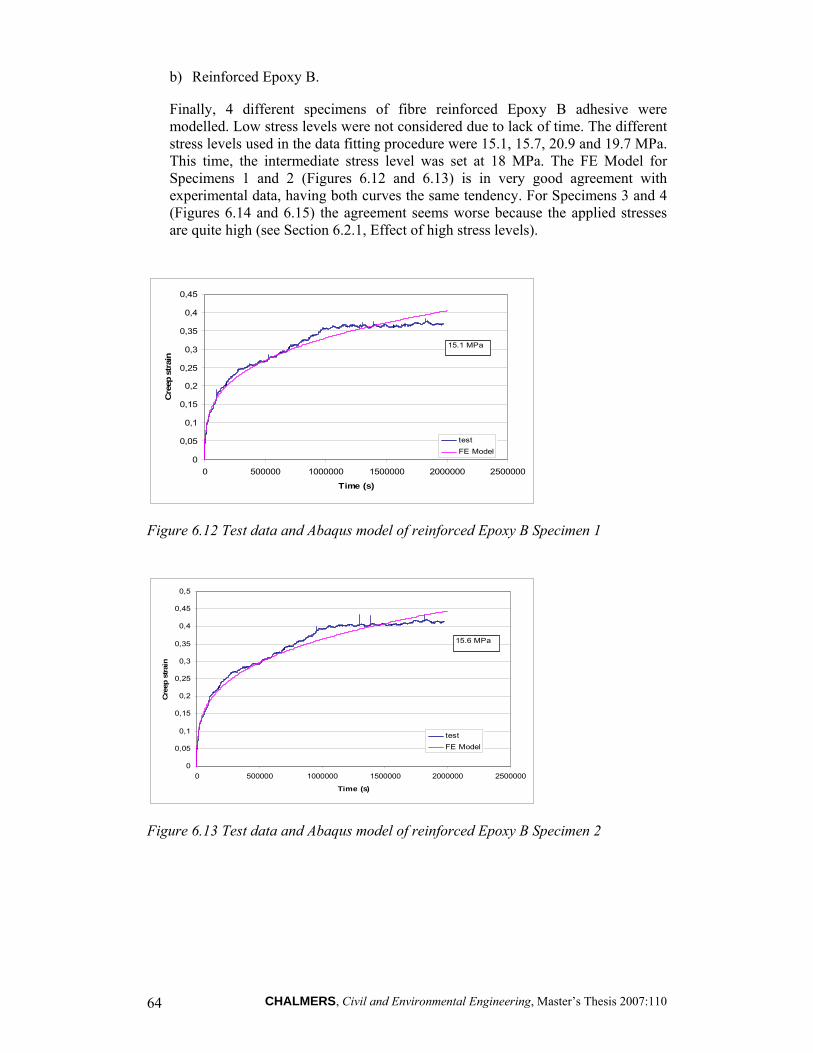
CHALMERS, Civil and Environmental Engineering, Master’s Thesis 2007:110 64
b) Reinforced Epoxy B.
Finally, 4 different specimens of fibre reinforced Epoxy B adhesive were modelled. Low stress levels were not considered due to lack of time. The different stress levels used in the data fitting procedure were 15.1, 15.7, 20.9 and 19.7 MPa. This time, the intermediate stress level was set at 18 MPa. The FE Model for Specimens 1 and 2 (Figures 6.12 and 6.13) is in very good agreement with experimental data, having both curves the same tendency. For Specimens 3 and 4 (Figures 6.14 and 6.15) the agreement seems worse because the applied stresses are quite high (see Section 6.2.1, Effect of high stress levels).
0
0,05
0,1
0,15
0,2
0,25
0,3
0,35
0,4
0,45
0 500000 1000000 1500000 2000000 2500000
Time (s)
Cre
ep s
trai
n
testFE Model
15.1 MPa
Figure 6.12 Test data and Abaqus model of reinforced Epoxy B Specimen 1
0
0,05
0,1
0,15
0,2
0,25
0,3
0,35
0,4
0,45
0,5
0 500000 1000000 1500000 2000000 2500000
Time (s)
Cree
p st
rain
testFE Model
15.6 MPa
Figure 6.13 Test data and Abaqus model of reinforced Epoxy B Specimen 2
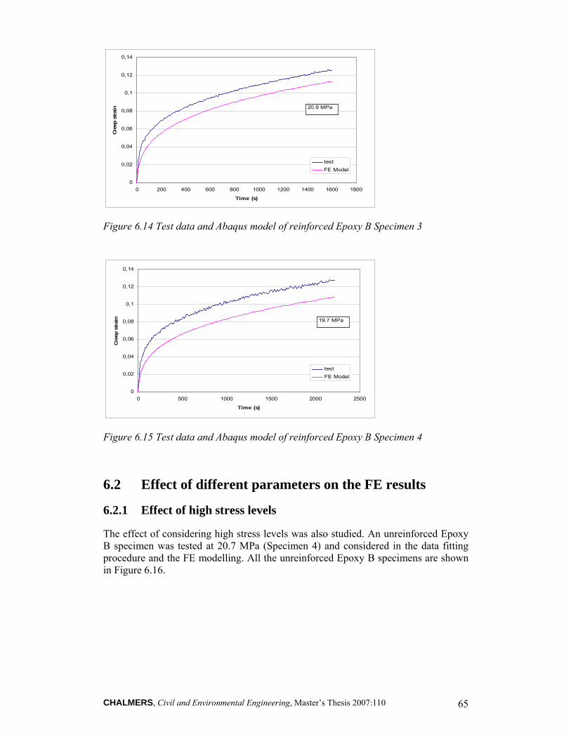
CHALMERS, Civil and Environmental Engineering, Master’s Thesis 2007:110 65
0
0,02
0,04
0,06
0,08
0,1
0,12
0,14
0 200 400 600 800 1000 1200 1400 1600 1800
Time (s)
Cree
p st
rain
testFE Model
20.9 MPa
Figure 6.14 Test data and Abaqus model of reinforced Epoxy B Specimen 3
0
0,02
0,04
0,06
0,08
0,1
0,12
0,14
0 500 1000 1500 2000 2500
Time (s)
Cree
p st
rain
testFE Model
19.7 MPa
Figure 6.15 Test data and Abaqus model of reinforced Epoxy B Specimen 4
6.2 Effect of different parameters on the FE results
6.2.1 Effect of high stress levels
The effect of considering high stress levels was also studied. An unreinforced Epoxy B specimen was tested at 20.7 MPa (Specimen 4) and considered in the data fitting procedure and the FE modelling. All the unreinforced Epoxy B specimens are shown in Figure 6.16.
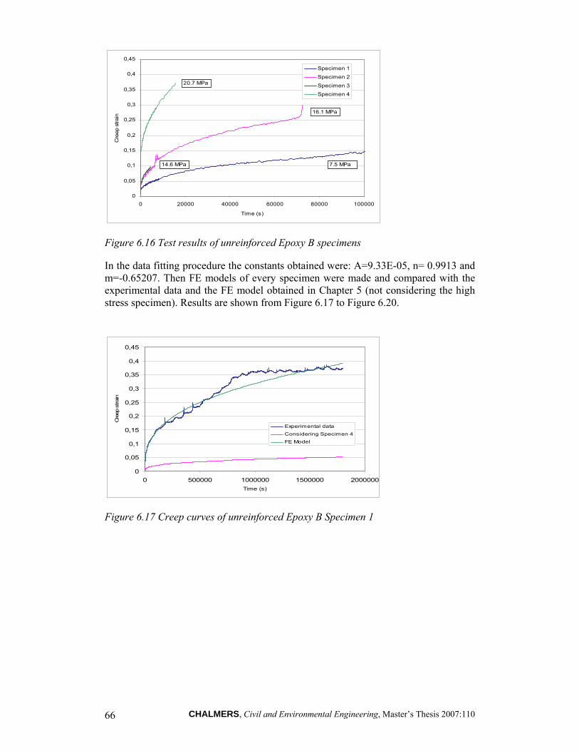
CHALMERS, Civil and Environmental Engineering, Master’s Thesis 2007:110 66
0
0,05
0,1
0,15
0,2
0,25
0,3
0,35
0,4
0,45
0 20000 40000 60000 80000 100000
Time (s)
Cre
ep s
train
Specimen 1Specimen 2
Specimen 3Specimen 4
20.7 MPa
14.6 MPa
16.1 MPa
7.5 MPa
Figure 6.16 Test results of unreinforced Epoxy B specimens
In the data fitting procedure the constants obtained were: A=9.33E-05, n= 0.9913 and m=-0.65207. Then FE models of every specimen were made and compared with the experimental data and the FE model obtained in Chapter 5 (not considering the high stress specimen). Results are shown from Figure 6.17 to Figure 6.20.
0
0,05
0,1
0,15
0,2
0,25
0,3
0,35
0,4
0,45
0 500000 1000000 1500000 2000000Time (s)
Cre
ep s
train
Experimental data
Considering Specimen 4
FE Model
Figure 6.17 Creep curves of unreinforced Epoxy B Specimen 1
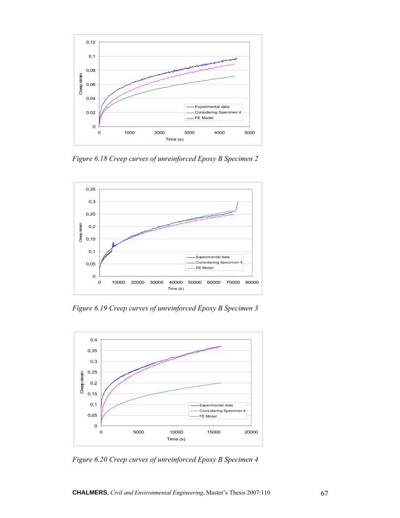
CHALMERS, Civil and Environmental Engineering, Master’s Thesis 2007:110 67
0
0,02
0,04
0,06
0,08
0,1
0,12
0 1000 2000 3000 4000 5000Time (s)
Cre
ep s
train
Experimental dataConsidering Specimen 4FE Model
Figure 6.18 Creep curves of unreinforced Epoxy B Specimen 2
0
0,05
0,1
0,15
0,2
0,25
0,3
0,35
0 10000 20000 30000 40000 50000 60000 70000 80000Time (s)
Cre
ep s
train
Experimental data
Considering Specimen 4
FE Model
Figure 6.19 Creep curves of unreinforced Epoxy B Specimen 3
0
0,05
0,1
0,15
0,2
0,25
0,3
0,35
0,4
0 5000 10000 15000 20000
Time (s)
Cre
ep s
train
Experimental data
Considering Specimen 4
FE Model
Figure 6.20 Creep curves of unreinforced Epoxy B Specimen 4
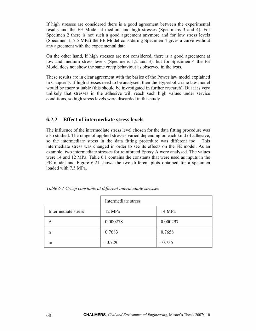
CHALMERS, Civil and Environmental Engineering, Master’s Thesis 2007:110 68
If high stresses are considered there is a good agreement between the experimental results and the FE Model at medium and high stresses (Specimens 3 and 4). For Specimen 2 there is not such a good agreement anymore and for low stress levels (Specimen 1, 7.5 MPa) the FE Model considering Specimen 4 gives a curve without any agreement with the experimental data.
On the other hand, if high stresses are not considered, there is a good agreement at low and medium stress levels (Specimens 1,2 and 3), but for Specimen 4 the FE Model does not show the same creep behaviour as observed in the tests.
These results are in clear agreement with the basics of the Power law model explained in Chapter 5. If high stresses need to be analysed, then the Hyperbolic-sine law model would be more suitable (this should be investigated in further research). But it is very unlikely that stresses in the adhesive will reach such high values under service conditions, so high stress levels were discarded in this study.
6.2.2 Effect of intermediate stress levels
The influence of the intermediate stress level chosen for the data fitting procedure was also studied. The range of applied stresses varied depending on each kind of adhesive, so the intermediate stress in the data fitting procedure was different too. This intermediate stress was changed in order to see its effects on the FE model. As an example, two intermediate stresses for reinforced Epoxy A were analysed. The values were 14 and 12 MPa. Table 6.1 contains the constants that were used as inputs in the FE model and Figure 6.21 shows the two different plots obtained for a specimen loaded with 7.5 MPa.
Table 6.1 Creep constants at different intermediate stresses
Intermediate stress
Intermediate stress 12 MPa 14 MPa
A 0.000278 0.000297
n 0.7683 0.7658
m -0.729 -0.735
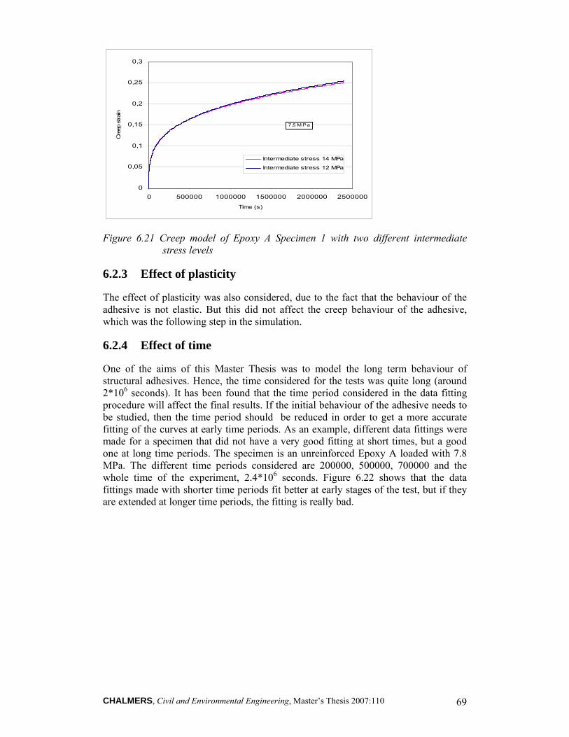
CHALMERS, Civil and Environmental Engineering, Master’s Thesis 2007:110 69
0
0,05
0,1
0,15
0,2
0,25
0,3
0 500000 1000000 1500000 2000000 2500000
Time (s)
Cre
ep s
train
Intermediate stress 14 MPa
Intermediate stress 12 MPa
7.5 M Pa
Figure 6.21 Creep model of Epoxy A Specimen 1 with two different intermediate stress levels
6.2.3 Effect of plasticity
The effect of plasticity was also considered, due to the fact that the behaviour of the adhesive is not elastic. But this did not affect the creep behaviour of the adhesive, which was the following step in the simulation.
6.2.4 Effect of time
One of the aims of this Master Thesis was to model the long term behaviour of structural adhesives. Hence, the time considered for the tests was quite long (around 2*106 seconds). It has been found that the time period considered in the data fitting procedure will affect the final results. If the initial behaviour of the adhesive needs to be studied, then the time period should be reduced in order to get a more accurate fitting of the curves at early time periods. As an example, different data fittings were made for a specimen that did not have a very good fitting at short times, but a good one at long time periods. The specimen is an unreinforced Epoxy A loaded with 7.8 MPa. The different time periods considered are 200000, 500000, 700000 and the whole time of the experiment, 2.4*106 seconds. Figure 6.22 shows that the data fittings made with shorter time periods fit better at early stages of the test, but if they are extended at longer time periods, the fitting is really bad.
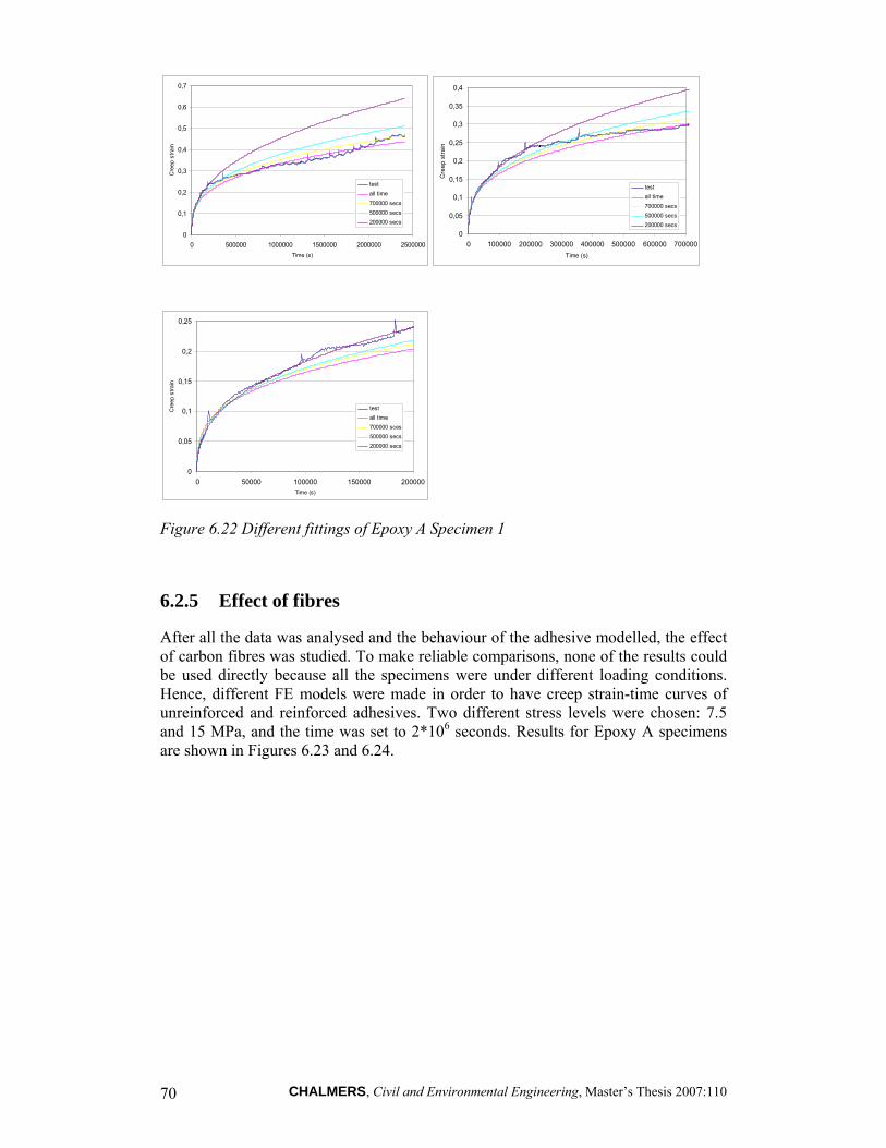
CHALMERS, Civil and Environmental Engineering, Master’s Thesis 2007:110 70
0
0,1
0,2
0,3
0,4
0,5
0,6
0,7
0 500000 1000000 1500000 2000000 2500000Time (s)
Cre
ep s
train
testall time700000 secs500000 secs200000 secs
0
0,05
0,1
0,15
0,2
0,25
0,3
0,35
0,4
0 100000 200000 300000 400000 500000 600000 700000Time (s)
Cre
ep s
train
testall time700000 secs500000 secs200000 secs
0
0,05
0,1
0,15
0,2
0,25
0 50000 100000 150000 200000Time (s)
Cre
ep s
train
testall time700000 sces500000 secs200000 secs
Figure 6.22 Different fittings of Epoxy A Specimen 1
6.2.5 Effect of fibres
After all the data was analysed and the behaviour of the adhesive modelled, the effect of carbon fibres was studied. To make reliable comparisons, none of the results could be used directly because all the specimens were under different loading conditions. Hence, different FE models were made in order to have creep strain-time curves of unreinforced and reinforced adhesives. Two different stress levels were chosen: 7.5 and 15 MPa, and the time was set to 2*106 seconds. Results for Epoxy A specimens are shown in Figures 6.23 and 6.24.
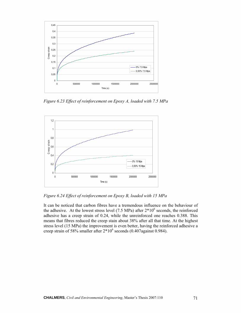
CHALMERS, Civil and Environmental Engineering, Master’s Thesis 2007:110 71
0
0,05
0,1
0,15
0,2
0,25
0,3
0,35
0,4
0,45
0 500000 1000000 1500000 2000000 2500000
Time (s)
Cre
ep s
train
0% 7,5 Mpa
0,50% 7,5 Mpa
Figure 6.23 Effect of reinforcement on Epoxy A, loaded with 7.5 MPa
0
0,2
0,4
0,6
0,8
1
1,2
0 500000 1000000 1500000 2000000 2500000
Time (s)
Cre
ep s
train
0% 15 Mpa
0,50% 15 Mpa
Figure 6.24 Effect of reinforcement on Epoxy B, loaded with 15 MPa
It can be noticed that carbon fibres have a tremendous influence on the behaviour of the adhesive. At the lowest stress level (7.5 MPa) after 2*106 seconds, the reinforced adhesive has a creep strain of 0.24, while the unreinforced one reaches 0.388. This means that fibres reduced the creep stain about 38% after all that time. At the highest stress level (15 MPa) the improvement is even better, having the reinforced adhesive a creep strain of 58% smaller after 2*106 seconds (0.407against 0.984).

CHALMERS, Civil and Environmental Engineering, Master’s Thesis 2007:110 72
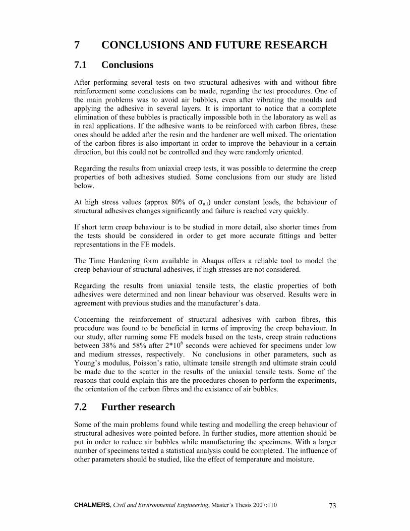
CHALMERS, Civil and Environmental Engineering, Master’s Thesis 2007:110 73
7 CONCLUSIONS AND FUTURE RESEARCH
7.1 Conclusions
After performing several tests on two structural adhesives with and without fibre reinforcement some conclusions can be made, regarding the test procedures. One of the main problems was to avoid air bubbles, even after vibrating the moulds and applying the adhesive in several layers. It is important to notice that a complete elimination of these bubbles is practically impossible both in the laboratory as well as in real applications. If the adhesive wants to be reinforced with carbon fibres, these ones should be added after the resin and the hardener are well mixed. The orientation of the carbon fibres is also important in order to improve the behaviour in a certain direction, but this could not be controlled and they were randomly oriented.
Regarding the results from uniaxial creep tests, it was possible to determine the creep properties of both adhesives studied. Some conclusions from our study are listed below.
At high stress values (approx 80% of σult) under constant loads, the behaviour of structural adhesives changes significantly and failure is reached very quickly.
If short term creep behaviour is to be studied in more detail, also shorter times from the tests should be considered in order to get more accurate fittings and better representations in the FE models.
The Time Hardening form available in Abaqus offers a reliable tool to model the creep behaviour of structural adhesives, if high stresses are not considered.
Regarding the results from uniaxial tensile tests, the elastic properties of both adhesives were determined and non linear behaviour was observed. Results were in agreement with previous studies and the manufacturer’s data.
Concerning the reinforcement of structural adhesives with carbon fibres, this procedure was found to be beneficial in terms of improving the creep behaviour. In our study, after running some FE models based on the tests, creep strain reductions between 38% and 58% after 2*106 seconds were achieved for specimens under low and medium stresses, respectively. No conclusions in other parameters, such as Young’s modulus, Poisson’s ratio, ultimate tensile strength and ultimate strain could be made due to the scatter in the results of the uniaxial tensile tests. Some of the reasons that could explain this are the procedures chosen to perform the experiments, the orientation of the carbon fibres and the existance of air bubbles.
7.2 Further research
Some of the main problems found while testing and modelling the creep behaviour of structural adhesives were pointed before. In further studies, more attention should be put in order to reduce air bubbles while manufacturing the specimens. With a larger number of specimens tested a statistical analysis could be completed. The influence of other parameters should be studied, like the effect of temperature and moisture.
CHALMERS, Civil and Environmental Engineering, Master’s Thesis 2007:110 74
The change in moisture content and changes in temperature, which are inevitable in exposed structures, should be studied in more detail if creep properties of adhesives want to be known completely. Besides, different fibre contents and fibre lengths should be investigated if the effect of reinforcing structural adhesives with fibres is to be studied with greater detail.
Further studies should include other existing models or user subroutines in FE programs if the whole range of stresses is to be modelled.
This study has provided some information about the creep properties of bulk adhesives. The next step should be the study of this behaviour in adhesive joints, based on the parameters obtained in this Master Thesis. Different joint tests (i.e. steel-CFRP lap joint tests) should be carried out and FE models should be used in order to investigate how creep affects the performance of adhesive joints. An interesting point to observe would be the redistribution of shear and peel stresses under constant loads.
CHALMERS, Civil and Environmental Engineering, Master’s Thesis 2007:110 75
8 References
ABAQUS Online Documentation. Version 6.6 http://abaqus.ethz.ch:2080/v6.6/
Augustsson C. (2004): NM Epoxy Handbook. Nils Malmgren AB, Ytterby, Sweden.
Buch X. (2000): Degradation Thermique et Fluage d’un Adhesif Structural Epoxyde. Ecole des Mines de Paris, France.
Charambalides M.N., Olusanya A. (1997): The Constitutive Models Suitable for Adhesives in some Finite Element Codes and Suggested Methods of Generating the Appropriate Materials Data. National Physical Laboratory, Teddington, United Kingdom
Dean G., Mera G. (2004): Modelling Creep in Toughened Adhesives for Finite Element Analysis. National Physical Laboratory, Teddington, United Kingdom.
De Castro San Román J. (2005): Experiments on Epoxy, Polyurethane and ADP Adhesives. Technical Report No. CCLab 2000.1b/1, École polytechnique Fédérale de Laussane, Switzerland.
Dillard D., Pocius A. (2002): The Mechanics of Adhesion. Elsevier, Amsterdam, The Netherlands.
Duncan B.C., Ogilvie-Robb K. (1999): Creep of Flexible Adhesive Joints. National Physical Laboratory, Teddington, United Kingdom.
Feng, C. (2004): Prediction of Long-Term Creep Behaviour of Epoxy Adhesives for Structural Applications. Texas A&M University, Texas, United States.
Gommersall E., Crocombe A.D., Smith P.A. (1996): MTS Adhesives Project 2: Report No. 6: Annex 5: Modelling the Response of Bonded Joints to Creep Loads. AEA Technology, Didcot, United Kingdom.
Gommersall E., Crocombe A.D., Smith P.A. (1995): MTS Adhesives Project 2: Failure Modes an Criteria, Report No. 6: Annex 4: The effect of Long Term Static Loading on Adhesives AV119 and F241. University of Surrey, Guildford, United Kingdom.
http://www.compositesiq.com/
Hu F., Olusanya A. (1997): Measurement of Creep and Stress Relaxation in Rubber and Rubber Type Materials. National Physical Laboratory, Teddington, United Kingdom.
Hugenschmidt F. (1982): New experiences with epoxies for structural application. Int. J. Adhesion and Adhesives, April 1982, pp. 84-95.
Hughes E., Rutherford J. (1979): Stress Dependence of Creep in Bonded Adhesives. Materials Science and engineering, 44 (1980), pp. 57-62.
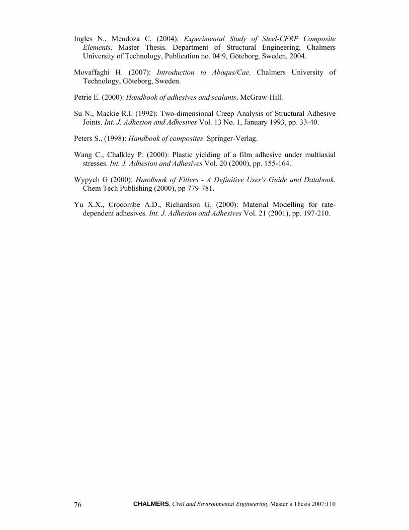
CHALMERS, Civil and Environmental Engineering, Master’s Thesis 2007:110 76
Ingles N., Mendoza C. (2004): Experimental Study of Steel-CFRP Composite Elements. Master Thesis. Department of Structural Engineering, Chalmers University of Technology, Publication no. 04:9, Göteborg, Sweden, 2004.
Movaffaghi H. (2007): Introduction to Abaqus/Cae. Chalmers University of Technology, Göteborg, Sweden.
Petrie E. (2000): Handbook of adhesives and sealants. McGraw-Hill.
Su N., Mackie R.I. (1992): Two-dimensional Creep Analysis of Structural Adhesive Joints. Int. J. Adhesion and Adhesives Vol. 13 No. 1, January 1993, pp. 33-40.
Peters S., (1998): Handbook of composites. Springer-Verlag.
Wang C., Chalkley P. (2000): Plastic yielding of a film adhesive under multiaxial stresses. Int. J. Adhesion and Adhesives Vol. 20 (2000), pp. 155-164.
Wypych G (2000): Handbook of Fillers - A Definitive User's Guide and Databook. Chem Tech Publishing (2000), pp 779-781.
Yu X.X., Crocombe A.D., Richardson G. (2000): Material Modelling for rate-dependent adhesives. Int. J. Adhesion and Adhesives Vol. 21 (2001), pp. 197-210.
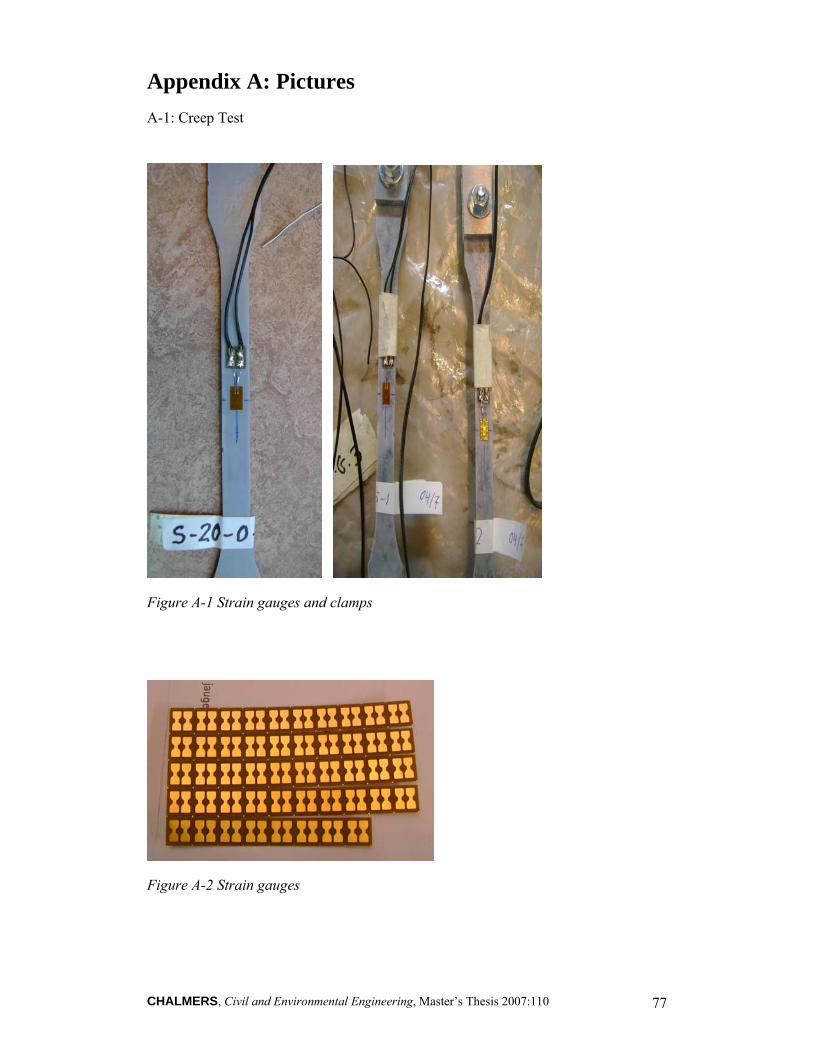
CHALMERS, Civil and Environmental Engineering, Master’s Thesis 2007:110 77
Appendix A: Pictures A-1: Creep Test
Figure A-1 Strain gauges and clamps
Figure A-2 Strain gauges
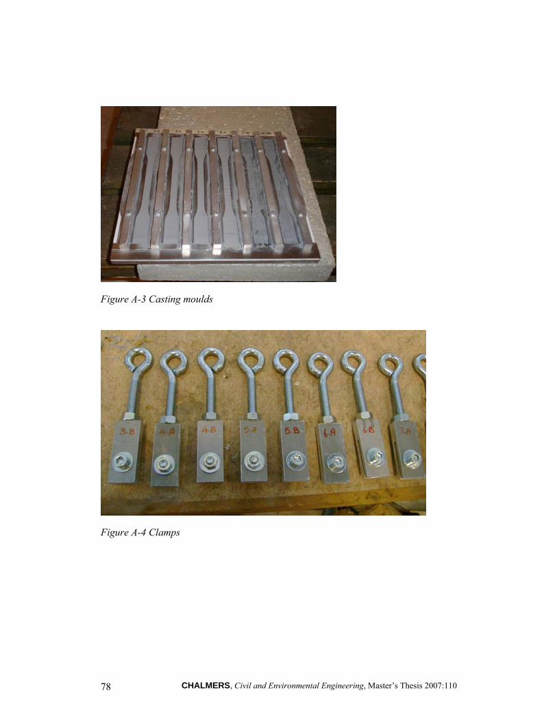
CHALMERS, Civil and Environmental Engineering, Master’s Thesis 2007:110 78
Figure A-3 Casting moulds
Figure A-4 Clamps
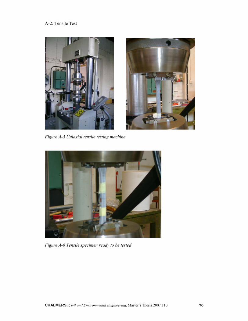
CHALMERS, Civil and Environmental Engineering, Master’s Thesis 2007:110 79
A-2: Tensile Test
Figure A-5 Uniaxial tensile testing machine
Figure A-6 Tensile specimen ready to be tested
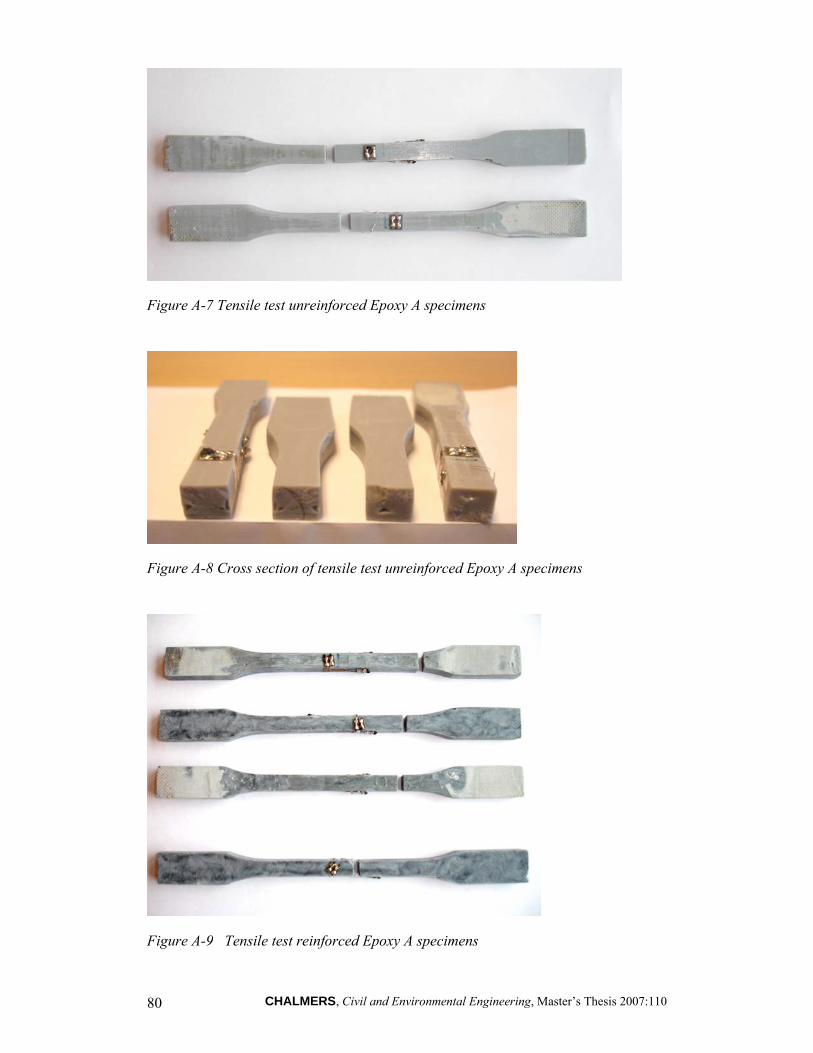
CHALMERS, Civil and Environmental Engineering, Master’s Thesis 2007:110 80
Figure A-7 Tensile test unreinforced Epoxy A specimens
Figure A-8 Cross section of tensile test unreinforced Epoxy A specimens
Figure A-9 Tensile test reinforced Epoxy A specimens
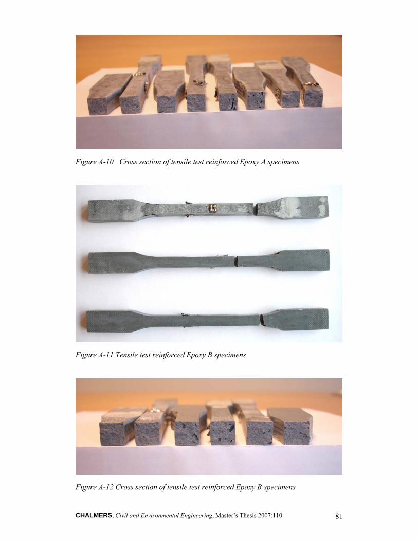
CHALMERS, Civil and Environmental Engineering, Master’s Thesis 2007:110 81
Figure A-10 Cross section of tensile test reinforced Epoxy A specimens
Figure A-11 Tensile test reinforced Epoxy B specimens
Figure A-12 Cross section of tensile test reinforced Epoxy B specimens
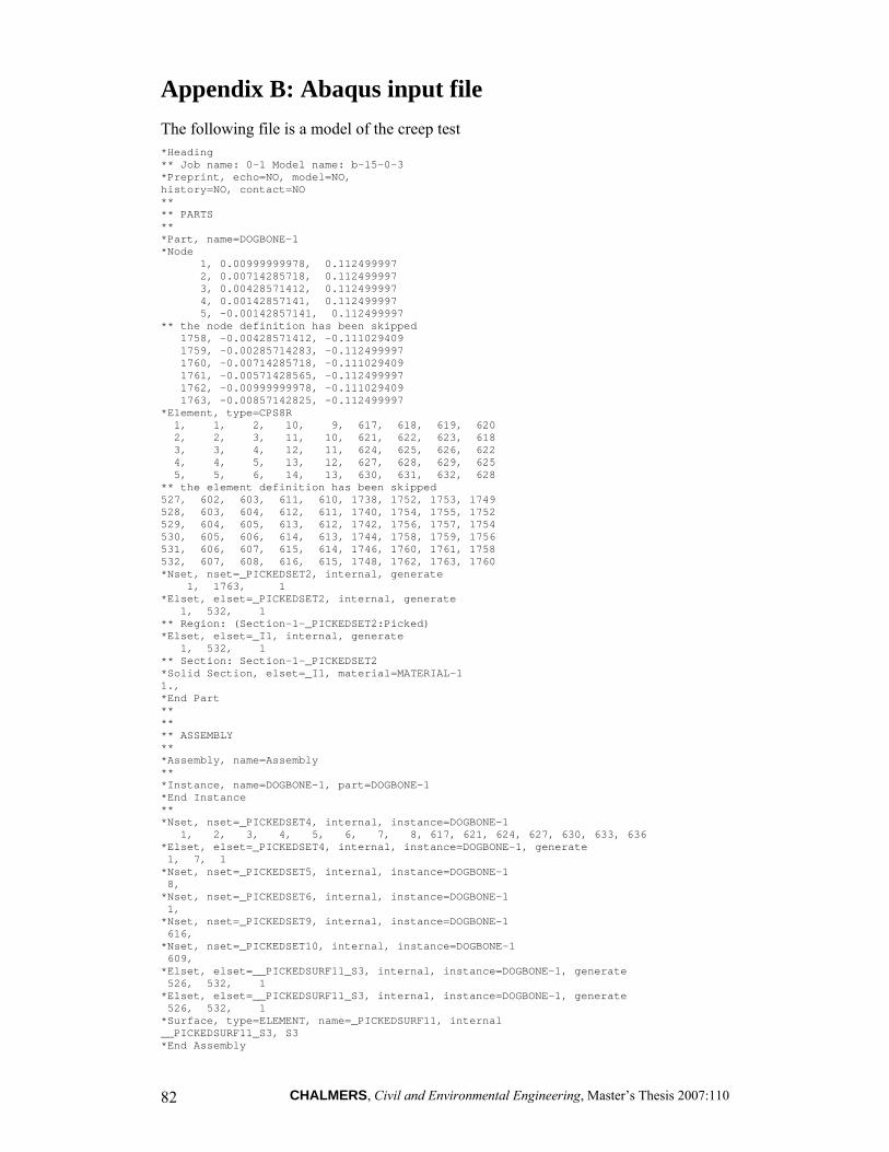
CHALMERS, Civil and Environmental Engineering, Master’s Thesis 2007:110 82
Appendix B: Abaqus input file The following file is a model of the creep test *Heading ** Job name: 0-1 Model name: b-15-0-3 *Preprint, echo=NO, model=NO, history=NO, contact=NO ** ** PARTS ** *Part, name=DOGBONE-1 *Node 1, 0.00999999978, 0.112499997 2, 0.00714285718, 0.112499997 3, 0.00428571412, 0.112499997 4, 0.00142857141, 0.112499997 5, -0.00142857141, 0.112499997 ** the node definition has been skipped 1758, -0.00428571412, -0.111029409 1759, -0.00285714283, -0.112499997 1760, -0.00714285718, -0.111029409 1761, -0.00571428565, -0.112499997 1762, -0.00999999978, -0.111029409 1763, -0.00857142825, -0.112499997 *Element, type=CPS8R 1, 1, 2, 10, 9, 617, 618, 619, 620 2, 2, 3, 11, 10, 621, 622, 623, 618 3, 3, 4, 12, 11, 624, 625, 626, 622 4, 4, 5, 13, 12, 627, 628, 629, 625 5, 5, 6, 14, 13, 630, 631, 632, 628 ** the element definition has been skipped 527, 602, 603, 611, 610, 1738, 1752, 1753, 1749 528, 603, 604, 612, 611, 1740, 1754, 1755, 1752 529, 604, 605, 613, 612, 1742, 1756, 1757, 1754 530, 605, 606, 614, 613, 1744, 1758, 1759, 1756 531, 606, 607, 615, 614, 1746, 1760, 1761, 1758 532, 607, 608, 616, 615, 1748, 1762, 1763, 1760 *Nset, nset=_PICKEDSET2, internal, generate 1, 1763, 1 *Elset, elset=_PICKEDSET2, internal, generate 1, 532, 1 ** Region: (Section-1-_PICKEDSET2:Picked) *Elset, elset=_I1, internal, generate 1, 532, 1 ** Section: Section-1-_PICKEDSET2 *Solid Section, elset=_I1, material=MATERIAL-1 1., *End Part ** ** ** ASSEMBLY ** *Assembly, name=Assembly ** *Instance, name=DOGBONE-1, part=DOGBONE-1 *End Instance ** *Nset, nset=_PICKEDSET4, internal, instance=DOGBONE-1 1, 2, 3, 4, 5, 6, 7, 8, 617, 621, 624, 627, 630, 633, 636 *Elset, elset=_PICKEDSET4, internal, instance=DOGBONE-1, generate 1, 7, 1 *Nset, nset=_PICKEDSET5, internal, instance=DOGBONE-1 8, *Nset, nset=_PICKEDSET6, internal, instance=DOGBONE-1 1, *Nset, nset=_PICKEDSET9, internal, instance=DOGBONE-1 616, *Nset, nset=_PICKEDSET10, internal, instance=DOGBONE-1 609, *Elset, elset=__PICKEDSURF11_S3, internal, instance=DOGBONE-1, generate 526, 532, 1 *Elset, elset=__PICKEDSURF11_S3, internal, instance=DOGBONE-1, generate 526, 532, 1 *Surface, type=ELEMENT, name=_PICKEDSURF11, internal __PICKEDSURF11_S3, S3 *End Assembly
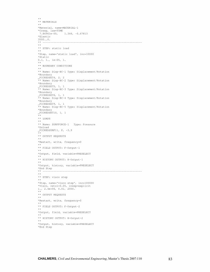
CHALMERS, Civil and Environmental Engineering, Master’s Thesis 2007:110 83
** ** MATERIALS ** *Material, name=MATERIAL-1 *Creep, law=TIME 7.86961e-05, 1.344, -0.67813 *Elastic 3500.,0. ** ---------------------------------------------------------------- ** ** STEP: static load ** *Step, name="static load", inc=10000 *Static 0.1, 1., 1e-05, 1. ** ** BOUNDARY CONDITIONS ** ** Name: Disp-BC-1 Type: Displacement/Rotation *Boundary _PICKEDSET4, 2, 2 ** Name: Disp-BC-2 Type: Displacement/Rotation *Boundary _PICKEDSET5, 1, 1 ** Name: Disp-BC-3 Type: Displacement/Rotation *Boundary _PICKEDSET6, 1, 1 ** Name: Disp-BC-4 Type: Displacement/Rotation *Boundary _PICKEDSET9, 1, 1 ** Name: Disp-BC-5 Type: Displacement/Rotation *Boundary _PICKEDSET10, 1, 1 ** ** LOADS ** ** Name: SURFFORCE-1 Type: Pressure *Dsload _PICKEDSURF11, P, -3.9 ** ** OUTPUT REQUESTS ** *Restart, write, frequency=0 ** ** FIELD OUTPUT: F-Output-1 ** *Output, field, variable=PRESELECT ** ** HISTORY OUTPUT: H-Output-1 ** *Output, history, variable=PRESELECT *End Step ** ---------------------------------------------------------------- ** ** STEP: visco step ** *Step, name="visco step", inc=100000 *Visco, cetol=0.05, creep=explicit 1., 2.4e+06, 0.01, 2000. ** ** OUTPUT REQUESTS ** *Restart, write, frequency=0 ** ** FIELD OUTPUT: F-Output-2 ** *Output, field, variable=PRESELECT ** ** HISTORY OUTPUT: H-Output-2 ** *Output, history, variable=PRESELECT *End Step
CHALMERS, Civil and Environmental Engineering, Master’s Thesis 2007:110 84
The following file is a model of the double lap joint *Heading creep ** Job name: Job-1 Model name: creep *Preprint, echo=NO, model=NO, history=NO, contact=NO ** ** PARTS ** *Part, name=PART-1 *Node 1, 848.661194, 398.792755 2, 848.661194, 398.959442 3, 848.661194, 399.126099 4, 848.661194, 399.292755 5, 848.661194, 399.459442 6, 848.661194, 399.626099 ** the definition of all the nodes is not included 5434, 565.661194, 410.792755 5436, 564.661194, 403.292755 5437, 564.661194, 405.792755 5438, 564.661194, 408.292755 5439, 564.661194, 410.792755 5441, 563.661194, 405.792755 5442, 563.661194, 410.792755 *Element, type=CPS8 1, 1, 3, 23, 21, 2, 15, 22, 14 2, 3, 5, 25, 23, 4, 16, 24, 15 3, 5, 7, 27, 25, 6, 17, 26, 16 4, 7, 9, 29, 27, 8, 18, 28, 17 ** the definition of all the elements is not included 1435, 1436, 1437, 1438, 1439, 1440, 1441, 1442, 1443, 1444, 1445, 1446, 1447, 1448, 1449, 1450 1451, 1452, 1453, 1454, 1455, 1456, 1457, 1458, 1459, 1460, 1461, 1462, 1463, 1464, 1465, 1466 1467, 1468, 1469, 1470, 1471, 1472, 1473, 1474, 1475, 1476, 1477, 1478, 1479, 1480, 1481, 1482 1483, 1484, 1485, 1486, 1487, 1488, 1489, 1490, 1491 *Elset, elset=PLANESTRESS1_3 1, 2, 3, 4, 5, 6, 7, 8, 9, 10, 11, 12, 13, 14, 15, 16 17, 18, 19, 20, 21, 22, 23, 24, 25, 26, 27, 28, 29, 30, 31, 32 33, 34, 35, 36, 37, 38, 39, 40, 41, 42, 43, 44, 45, 46, 47, 48 49, 50, 51, 52, 53, 54, 55, 56, 57, 58, 59, 60, 61, 62, 63, 64 65, 66, 67, 68, 69, 70, 71, 72, 73, 74, 75, 76, 77, 78, 79, 80 81, 82, 83, 84, 85, 86, 87, 88, 89, 90, 91, 92, 93, 94, 95, 96 97, 98, 99, 100, 101, 102, 103, 104, 105, 106, 107, 108, 110, 113, 115, 116 ** not everything included 357, 358, 359, 360, 361, 362, 363, 364, 365, 366, 367, 368, 369, 370, 371, 372 373, 374, 375, 376, 377, 378, 379, 380, 381, 382, 383, 384, 386, 389, 391, 392 393, 394, 395, 396, 397, 398, 399, 400, 401, 402, 403, 404, 405, 406, 407, 408 409, 410, 411, 412, 413, 414, 415, 416, 417, 418, 419, 420, 421, 422, 423, 424 425, 426, 427, 428, 429, 430, 431, 432, 433, 434, 435, 436, 437, 438, 439, 440 441, 442, 443, 444, 445, 446, 447, 448, 449, 450, 451, 452 ** Region: (Section-4-PLANESTRESS1_3:PLANESTRESS1_3), (Controls:EC-1) ** Section: Section-4-PLANESTRESS1_3 *Solid Section, elset=PLANESTRESS1_3, controls=EC-1, material=ADHESIVE 50., ** Region: (Section-2-PLANESTRESS1_1:PLANESTRESS1_1), (Controls:EC-1) ** Section: Section-2-PLANESTRESS1_1 *Solid Section, elset=PLANESTRESS1_1, controls=EC-1, material=ADHESIVE 50., ** Region: (Section-3-PLANESTRESS1_2:PLANESTRESS1_2), (Controls:EC-1) ** Section: Section-3-PLANESTRESS1_2 *Solid Section, elset=PLANESTRESS1_2, controls=EC-1, material=GENERIC_ISOTROPIC_STEEL 50., ** Region: (Section-1-PLANESTRESS1:PLANESTRESS1), (Controls:EC-1) ** Section: Section-1-PLANESTRESS1 *Solid Section, elset=PLANESTRESS1, controls=EC-1, material=GENERIC_ISOTROPIC_STEEL 50., *End Part ** ** ** ASSEMBLY ** *Assembly, name=Assembly ** *Instance, name=PART-1-1, part=PART-1
CHALMERS, Civil and Environmental Engineering, Master’s Thesis 2007:110 85
*End Instance ** *Nset, nset=ALLNODES, instance=PART-1-1 1, 2, 3, 4, 5, 6, 7, 8, 9, 10, 11, 12, 13, 14, 15, 16 17, 18, 19, 20, 21, 22, 23, 24, 25, 26, 27, 28, 29, 30, 31, 32 33, 34, 35, 36, 37, 38, 39, 40, 41, 42, 43, 44, 45, 46, 47, 48 49, 50, 51, 52, 53, 54, 55, 56, 57, 58, 59, 60, 61, 62, 63, 64 65, 66, 67, 68, 69, 70, 71, 72, 73, 74, 75, 76, 77, 78, 79, 80 81, 82, 83, 84, 85, 86, 87, 88, 89, 90, 91, 92, 93, 94, 95, 96 ********** 4599, 4602, 4607, 4610, 4615, 4618, 4623, 4626, 4631, 4634, 4639, 4642, 4647, 4650, 4655, 4658 4663, 4666, 4671, 4674, 4679, 4682, 4687, 4690, 4695, 4698, 4703, 4706, 4711, 4714, 4719, 4722 4727, 4730, 4735, 4738, 4743, 4746, 4751, 4754, 4759, 4762, 4767, 4770, 4775, 4778, 4783, 4786 4791, *Nset, nset=BS000002, instance=PART-1-1, generate 3058, 3062, 1 *Nset, nset=_PickedSet8, internal, instance=PART-1-1 1700, 1701, 1702, 1703, 1704, 1705, 1706, 1707, 1708, 1709, 1710, 1711, 1712, 1713, 1714, 1715 1716, 1717, 1718, 1719, 1720, 2193, 2194, 2195, 2196, 2197, 2198, 2199, 2200, 2201, 2202, 2804 2817, 2824, 2837, 2844, 2857, 2864, 2877, 2884, 2897, 2904, 2917, 2924, 2937, 2944, 2957, 2964 2969, 2972, 2977, 2985, 2990, 2993, 2998, 3001, 3006, 3009, 3014, 3017, 3022, 3025, 3030, 3033 3038, 3041, 3046, 3049, 3054, 3057, 3062, 3063, 3076, 3083, 3096, 3103, 3116, 3123, 3136, 3143 ** not everything included 4735, 4738, 4743, 4746, 4751, 4754, 4759, 4762, 4767, 4770, 4775, 4778, 4783, 4786, 4791 *Nset, nset=_PickedSet9, internal, instance=PART-1-1, generate 3058, 3062, 1 *Elset, elset=__PickedSurf7_S3, internal, instance=PART-1-1 1114, 1115 *Surface, type=ELEMENT, name=_PickedSurf7, internal __PickedSurf7_S3, S3 *End Assembly ** ** ELEMENT CONTROLS ** *Section Controls, name=EC-1, DISTORTION CONTROL=NO, hourglass=STIFFNESS 1., 1., 1. ** ** MATERIALS ** *Material, name=ADHESIVE *Conductivity 45., *Creep, law=TIME 2.31e-06, 2.483, -0.699 *Density 7.82e-09, *Elastic 7000., 0.3 *Plastic 7.1, 0. 10.2, 0.00163 15., 0.00253 17., 0.00303 19.1, 0.00371 20.8, 0.00451 21.9, 0.00513 23.3, 0.00602 24.7, 0.00709 26., 0.00823 *Expansion, zero=21.85 1.17e-05, *Material, name=GENERIC_ISOTROPIC_STEEL *Conductivity 45.,

CHALMERS, Civil and Environmental Engineering, Master’s Thesis 2007:110 86
*Density 7.82e-09, *Elastic 206800., 0.29 *Expansion, zero=21.85 1.17e-05, ** ** PHYSICAL CONSTANTS ** *Physical Constants, absolute zero=-273.15, stefan boltzmann=5.6696e-11 ** ---------------------------------------------------------------- ** ** STEP: elastic ** *Step, name=elastic *Static 1., 1., 1e-05, 1. ** ** BOUNDARY CONDITIONS ** ** Name: BC-1 Type: Displacement/Rotation *Boundary _PickedSet8, 2, 2 ** Name: BC-2 Type: Displacement/Rotation *Boundary _PickedSet9, 1, 1 _PickedSet9, 2, 2 _PickedSet9, 6, 6 ** ** LOADS ** ** Name: Load-1 Type: Pressure *Dsload _PickedSurf7, P, -50. ** ** OUTPUT REQUESTS ** *Restart, write, frequency=0 ** ** FIELD OUTPUT: F-Output-1 ** *Output, field, variable=PRESELECT ** ** HISTORY OUTPUT: H-Output-1 ** *Output, history, variable=PRESELECT *End Step ** ---------------------------------------------------------------- ** ** STEP: visco step ** *Step, name="visco step", inc=10000 *Visco, cetol=0.05, creep=explicit 1., 5000., 0.1, 200. ** ** OUTPUT REQUESTS ** *Restart, write, frequency=0 ** ** FIELD OUTPUT: F-Output-1 ** *Output, field, variable=PRESELECT ** ** HISTORY OUTPUT: H-Output-1 ** *Output, history, variable=PRESELECT *End Step