The CPT Theorem - University of Oxfordusers.ox.ac.uk/~mert2255/papers/cpt.pdf · C1(M;C) thatassignstoevery 2Kafixedpolynomialcombinationofitsderived components–thatis,afinitesumoffiniteproductsofthem,alongwithcomplex

The CPT Theorem

Hilary Greaves and Teruji Thomas

Abstract. We provide a rigorous proof of the CPT theorem within the frame-work of ’Lagrangian’ quantum field theory. This is in contrast to the usual rig-orous proofs in purely axiomatic frameworks, and non-rigorous proof-sketcheswithin the Lagrangian framework.

1. Introduction and Motivation

The CPT theorem says, roughly, that every relativistic quantum field theoryhas a symmetry that simultaneously reverses charge (C), reverses the orientation ofspace (or ‘parity,’ P), and reverses the direction of time (T). In this paper we willstate and prove a general version of this theorem, proceeding from first principlesand explicitly setting out all required assumptions.

Why re-examine a result that is so widely known? The motivation stems fromthe fact that, as a general rule, the QFT literature splits rather sharply into twosectors. The first sector deals with ‘Lagrangian QFT’; it speaks the language ofmainstream particle physics, but is often rather relaxed about mathematical rigour.The second sector is fully rigorous, but bears a much looser relationship to the QFTsthat actually enjoy predictive success; it includes the axiomatic program of Streaterand Wightman, and the purely algebraic approach (AQFT) associated with e.g.Araki, Haag and Kastler. This contrast has been a focus of recent discussion inthe foundations community, with Doreen Fraser (?, ?) arguing that because of thelack of rigour in the mainstream approach, the axiomatic and algebraic frameworksprovide the more appropriate locus for foundational work, while David Wallace (?,?) advocates more foundational focus on the Lagrangian framework for the sake ofcontact with real physics.

The literature on the CPT theorem is no exception to this general rule. Instandard Lagrangian-QFT textbooks (e.g. (Peskin & Schroeder, 1995), (Itzykson &Zuber, 2005), (Weinberg, 19xx)) the ‘theorem’ is that Lagrangians of a certain kindare necessarily invariant under a CPT transformation of the fields; they establishthis result via case-by-case calculations for the fields of most physical interest (e.g.vectors or Dirac spinors in 3+1 spacetime dimensions), and refer the reader to e.g.(Streater & Wightman, 1964) for a more rigorous and general proof. If one followsup these references, one indeed finds a fully rigorous proof of a result called ‘CPTTheorem,’ but the relationship of that result to the CPT invariance of Lagrangiansis obscure; the same remark applies to such AQFT results as that presented in (?,

1

2 HILARY GREAVES AND TERUJI THOMAS

?). The literature contains a gap: there is no rigorous, general proof available ofthe CPT theorem within the framework of Lagrangian QFT.

Driven by the platitude that both mathematical rigour and contact with realphysics are highly desirable, this paper aims to fill that gap. We present a rigorousproof using only the basic geometric and group-theoretic facts on which the CPTresult essentially depends. Our approach has the following features.

(1) We are concerned solely with the symmetries of Lagrangian densities, dy-namical equations, and similar objects; we say only enough about quantum fieldtheory per se to motivate appropriate transformation laws. In fact, our resultsapply formally to classical relativistic field theories just as well as to quantum ones.We find that the quantum CPT theorem is an instance of a more general result,other instances of which can be seen as classical PT, classical CPT and quantum PTtheorems. In standard approaches to the CPT theorem, the relationship betweenquantum and classical symmetries is left unclear.

(2) We give a general construction of CPT transformations for an arbitraryfield, based only on how that field transforms under proper orthochronous Lorentztransformations. This construction is clearly tied to the requirements of our proofof the CPT theorem, so it is clear why an invariance theorem results for theseparticular transformations. In the existing Lagrangian-QFT literature, the CPTtransformations tend to be introduced ad hoc and case-by-case.

(3) We rely on a few basic geometric properties of the Lorentz group, so thatour results are valid for Minkowski space, and, indeed, for any non-Euclidean sig-nature, in dimension at least three. These properties are absent in dimension twoand for Galilean spacetimes (for which we show there is no analogous result). Thestandard approach relies on a detailed classification of the representations and in-variants of the four-dimensional Lorentz group, thus obscuring the basic structureand generality of the result.

(4) Our key technique is passage from the real to the complex Lorentz group.This ‘complexification’ is also the key idea used to prove the CPT theorem ofaxiomatic QFT, but it plays no overt role in standard approaches to the LagrangianCPT theorem.1

The present paper may also be of interest to those seeking a foundationalunderstanding of the prima facie mysterious connection between charge conjugationand spacetime symmetries that is embodied in the CPT theorem (cf. (Greaves,2007; ?, ?)).

We develop our argument pedagogically, treating first the simpler case of fieldstaking values in true representations of the Lorentz group (i.e. tensor fields), andlater generalising to include properly projective representations (spinor fields). Thereader interested only in the broad outline of our results can skip sections 5–9.

The structure of the paper is as follows. Sections 2–4 lay the conceptual founda-tions. Section 2 introduces our basic notion of a ‘formal field theory,’ and explainshow it can be used to study the symmetries of classical and quantum field theories.Section 3 explains the distinction between PT and CPT transformations, and therelated idea of charge conjugation. Section 4 uses this framework to give a detailedoverview of our results.

1Complexification does play a key role in the treatment of tensors in an illuminating paper byJ. S. Bell (1955); the latter was the original inspiration for the present paper.

THE CPT THEOREM 3

Sections 5–9 form the technical heart of the paper. Section 5 states and provesa ‘classical PT theorem’: we show that for classical field theories whose dynami-cal fields take values exclusively in true representations of the Lorentz group (thusexcluding spinor fields), proper orthochronous Lorentz invariance entails ‘PT invari-ance.’ Section 6 generalises the result of section 5: we prove a general invariancetheorem that has ‘tensors-only’ versions of the classical PT theorem, the quan-tum CPT theorem, and classical CPT and quantum PT theorems as corollaries.Of these, the classical PT and quantum CPT theorems are the most interesting,because their premisses are widely accepted.

We next generalise to spinorial field theories. Section 7 lays out the basic factsconcerning covers of the proper Lorentz group. Section 8 explains how the moststraightforward attempt to generalise our classical tensorial PT theorem to includespinors fails. Section 9, building on this instructive failure, further generalisesthe results of section 6 to the spinorial case; this includes the full quantum CPTtheorem.

Section 10 examines how our methods apply beyond Minkowski space. Wegeneralise our results to arbitrary non-Euclidean signatures in dimension at least 3.We also point out why our methods fail in various settings where there is provablyno analogue of the CPT theorem. Section 11 is the conclusion.

Some mathematical background is presented in Appendix A, to which thereader should refer as necessary. Appendix B relates our treatment of the coveringgroups of the Lorentz group to the usual approach in terms of Clifford algebras.Detailed proofs are relegated to Appendix C.

2. Field Theories and Their Symmetries

We will state and prove our invariance theorems in a setting of ‘formal fieldtheories,’ in which the objects of study are formal polynomials that can equally wellbe interpreted as dynamical equations or as defining Lagrangian or Hamiltoniandensities for classical or quantum field theories. The advantage of this framework(over, say, one that takes the objects of study to be spaces of kinematically allowedfields and their automorphisms) is its neutrality between classical and quantum fieldtheories, and between various interpretations of QFTs (as dynamical constraints onoperator-valued distributions, formal algorithms for the generation of transitionamplitudes, or anything else).

In this section we explain in detail what a formal field theory is, and howthey can be used to describe classical and quantum field theories. In particular,we explain how to analyse space-time symmetries of classical and quantum fieldtheories in terms of an analogous notion for formal field theories.

Initially, ‘spacetime’ M can be any vector space.2 We must eventually supposethat M has enough structure for us to speak of ‘time-reversing’ transformations.

2As a matter of convenience, we choose an origin forM (thus making it a vector space insteadof an affine space). When we discuss symmetries, this choice allows us to focus on the Lorentzgroup rather than the full Poincaré group; it is justified by an implicit assumption that our fieldtheories are, in an appropriate sense, translation invariant.


2.1. Classical field theories. A classical field theory is a set D ⊂ K, wherethe set K ≡ C∞(M,V ) of kinematically allowed fields consists of all smooth func-tions from spacetime to some finite-dimensional real vector space V .3 D is the setof dynamically allowed fields. We are mainly interested in theories D that con-sist of the solutions to a system of differential equations with constant coefficients– for brevity, we say that D is polynomial, because these field equations dependpolynomially on the field components and their derivatives.

We will allow our differential equations to have complex coefficients. Thisrequires some comment. If we were only interested in classical field theories, itwould suffice to consider differential equations with real coefficients. By way ofexample, it is true that the Dirac equation

(1) −iγµ∂µψ +mψ = 0

has complex coefficients; however, by taking real and imaginary parts, we mayconsider this as a system of two differential equations with real coefficients. Asthe example also shows, however, it is nevertheless convenient to allow for complexcoefficients, of which real coefficients are a special case. More importantly, the useof complex coefficients will be crucial for the study of symmetries in quantum fieldtheory. There the complex structure of the coefficients can be identified with thecomplex structure of Hilbert space, but must be sharply distinguished from anycomplex structure that V may happen to possess (e.g. the way in which a complexscalar field or a Dirac spinor is complex). The latter structure is fundamentallyirrelevant to our purposes (cf. Example 4).

We now spell out the notion of a polynomial classical field theory more precisely.First, let W = Hom(V,C) be the space of real-linear maps V → C. Given Φ ∈ K,by a derived component of Φ we mean one of the functions

(2) Φλξ1···ξn := ∂ξ1 · · · ∂ξn(λ ◦ Φ) ∈ C∞(M,C)

specified by the data of λ ∈ W and a (possibly empty) list of vectors ξ1, . . . , ξn ∈M . A differential operator (with constant complex coefficients) is a map K →C∞(M,C) that assigns to every Φ ∈ K a fixed polynomial combination of its derivedcomponents – that is, a finite sum of finite products of them, along with complexscalars. We say that a classical field theory D ⊂ K is polynomial if there is a setDdiff of differential operators such that

(3) Φ ∈ D ⇐⇒ [D(Φ) = 0 for all D ∈ Ddiff ].

The vast majority of classical field theories considered in physics are polynomial inthis sense.

Example 1. Consider the Maxwell equation usually written (with implicitsummation over β) as

(4) Fαβ,β − Jα = 0.

3If the theory ‘contains two or more dynamical fields,’ as e.g. electromagnetic theory containsthe Maxwell-Faraday tensor field Fαβ and the charge-current density vector field Jα, then V willnaturally be written as a direct sum of two or more spaces: VEM := VF ⊕ VJ . See Example 1.

THE CPT THEOREM 5

To illustrate our notation, let VF ⊂ M ⊗M be the space of contravariant4, skew-symmetric rank-two tensors at a point, and VJ = M the space of vectors. Apair consisting of a particular Maxwell-Faraday tensor field F ∈ C∞(M,VF ) and aparticular charge-current density vector field J ∈ C∞(M,VJ) can then be seen asa single field Φ ≡ F ⊕ J ∈ C∞(M,VF ⊕ VJ). With respect to an orthonormal basise0, e1, e2, e3 ∈M∗ of covectors, we can rewrite (4) as

(5) Φeαeβ⊕0

eβ− Φ0⊕eα = 0.

For each α ∈ {0, 1, 2, 3}, the left-hand side of (5) is a differential operator appliedto the field Φ = F ⊕ J ; the set Ddiff of these four operators specifies the dynamicsof Maxwell field theory, which is therefore a polynomial field theory.

Example 2. Here are two standard examples of non-polynomial field theories.First, consider the Sine-Gordon equation for a scalar field φ:

∂µ∂µφ+ sinφ = 0.

Since sine is not a polynomial function, this does not define a polynomial fieldtheory. However, our results could be extended (or applied indirectly) to the Sine-Gordon equation and similar cases in which the field equations involve power series(e.g. the Taylor series of sine) rather than polynomials.

A second type of example is a ‘non-linear σ model,’ in which the target spaceV is not even a vector space, but a manifold. If V is an algebraic variety, then thereis still a notion of ‘polynomial field theory,’ and it should be possible to extend ourresults in at least some cases. However, in this paper we will only consider the mostimportant case of polynomial field theories with a linear target space.

2.2. Formal field theories. We now shift attention from differential oper-ators to the formulae that define them. This abstraction will allow us to treatclassical and quantum field theories on the same footing.

A differential formula is a polynomial combination of the derived componentsof a purely symbolic field Φ. We call these derived components field symbols. Adifferential formula F determines a differential operator DF that assigns to eachclassical field Φ ∈ K the same polynomial combination of its derived components.

Let Kform be the set of all differential formulae. To be quite precise, we under-stand each field symbol Φλξ1···ξn as an element λ⊗ (ξ1 · · · ξn) of the complex vectorspace W ⊗R TM , where TM is the tensor algebra of M . Then we formally defineKform to be the free algebra Kform = F(W ⊗R TM) (see Appendix A.6–A.7).

Our basic objects of study are certain nice sets of differential formulae:Definition 1. A formal field theory is a complex affine subspaceDform ⊂ Kform

(see Appendix A.1).Thus a formal field theory Dform defines a polynomial classical field theory D

via

(6) Φ ∈ D ⇐⇒ [DF (Φ) = 0 for all F ∈ Dform].

Conversely, given a polynomial classical field theory D, we obtain a formal fieldtheory Dform as the largest collection of differential formulae F satisfying (6). Inthis case, Dform is actually a complex subspace of Kform.

4Since the Maxwell-Faraday tensor is the exterior derivative of a one-form, it is of course mostfundamentally a covariant anti-symmetric rank two tensor. We ignore this nicety for simplicity ofexposition; the background Minkowski metric allows us to raise and lower indices at will.


But this is only one way of interpreting formal field theories. We have sofar noted that a single differential formula F determines a dynamical equationDF (Φ) = 0; but we could instead consider DF as a Lagrangian or Hamiltoniandensity, from which dynamical equations are to be derived. In this case, we cantake Dform to be the set of all differential formulae defining the same density I.This is not a complex subspace of Kform, since it does not contain zero (unlessI = 0); but it is still a complex affine subspace.

Moving beyond classical field theories, an important feature of our definition isthat Kform is a non-commutative algebra. For example, given λ, µ ∈ W , the prod-ucts ΦλΦµ and ΦµΦλ are generally different elements of Kform – different formulae– even though ΦλΦµ = ΦµΦλ for any Φ ∈ K. By maintaining this distinction, weleave open the possibility of taking Φ to represent a quantum field, whose compo-nents do not generally commute.5

This is exactly what is done in standard approaches to QFT, where the ‘theory’is specified by a density I, presented, as in the classical case, by a differentialformula. How exactly I is interpreted may depend on whether we are interested incanonical quantization, path integrals, or other methods; but these questions arelargely irrelevant insofar as we can focus not on I itself, but on the collection Dform

of all differential formulae that define it. (We make these comments more precisein section 2.4.)

Thus the formal field theory approach is broadly neutral about what kind offield theories we wish to study (classical or quantum?) and about how we wishto study them. (Lagrangians, Hamiltonians, or dynamical equations? Operatordistributions or path integrals?). Because we are interested in symmetries of fieldtheories, the only general requirement is that the theory of interest D is specifiedby a complex affine subspace Dform ⊂ Kform, in such a way that symmetries of Dcorrespond to some appropriate notion of symmetries for Dform. Our next task isto explain just what the appropriate notions are.

2.3. Classical spacetime symmetries. First let us consider the situationfor classical field theories. A permutation of K is a symmetry of D if it leaves Dinvariant. One typically studies groups of symmetries: if a group G acts on K, wecan ask whether G acts by symmetries, i.e. whether D is G-invariant.

We are particularly interested in spacetime symmetries. This means that theaction u of G on K is determined by the data of a representation (ω,G,M) of G onM and a representation (ρ,G, V ) of G on V (cf. A.3 on representations). Namely,

(7) u(g)Φ = ρ(g) ◦ Φ ◦ ω(g−1) ∀g ∈ G,Φ ∈ K.

We summarize this situation by saying that G acts geometrically via, and that u isthe geometric action corresponding to, ρ and ω.6

Example 3. The basic example is when G is a subgroup of the Lorentz group(or, later, a covering group of such a subgroup); G then acts naturally on M ,so to get a geometric action, it remains to specify a representation of G on V .

5It is also possible to make sense of non-commutative classical fields in various ways – see ourdiscussion of supercommutativity in section 9.

6This characterisation of spacetime symmetries in terms of geometric actions is general enoughto include what are normally called ‘global internal symmetries’ – these come from geometricactions in which ω is the trivial representation.

THE CPT THEOREM 7

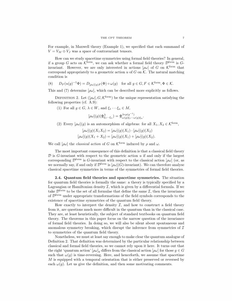
For example, in Maxwell theory (Example 1), we specified that each summand ofV = VM ⊕ VJ was a space of contravariant tensors.

How can we study spacetime symmetries using formal field theories? In general,if a group G acts on Kform, we can ask whether a formal field theory Dform is G-invariant. However, we are only interested in actions [ρω] of G on Kform thatcorrespond appropriately to a geometric action u of G on K. The natural matchingcondition is

(8) DF (u(g)−1Φ) = D[ρω](g)F (Φ) ◦ ω(g) for all g ∈ G,F ∈ Kform,Φ ∈ K.

This and (7) determine [ρω], which can be described more explicitly as follows.

Definition 2. Let ([ρω], G,Kform) be the unique representation satisfying thefollowing properties (cf. A.9):

(1) For all g ∈ G, λ ∈W , and ξ1 · · · ξn ∈M,

[ρω](g)(Φλξ1···ξn) = Φλ◦ρ(g−1)ω(g)ξ1···ω(g)ξn

.

(2) Every [ρω](g) is an automorphism of algebras: for all X1, X2 ∈ Kform,

[ρω](g)(X1X2) = [ρω](g)(X1) · [ρω](g)(X2)

[ρω](g)(X1 +X2) = [ρω](g)(X1) + [ρω](g)(X2).

We call [ρω] the classical action of G on Kform induced by ρ and ω.

The most important consequence of this definition is that a classical field theoryD is G-invariant with respect to the geometric action u if and only if the largestcorresponding Dform is G-invariant with respect to the classical action [ρω] (or, aswe normally say, if and only if Dform is [ρω](G)-invariant). We can therefore analyseclassical spacetime symmetries in terms of the symmetries of formal field theories.

2.4. Quantum field theories and spacetime symmetries. The situationfor quantum field theories is formally the same: a theory is typically specified by aLagrangian or Hamiltonian density I, which is given by a differential formula. If wetake Dform to be the set of all formulae that define the same I, then the invarianceof Dform under appropriate transformations of the field symbols corresponds to theexistence of spacetime symmetries of the quantum field theory.

How exactly to interpret the density I, and how to construct a field theoryfrom it, are questions much more difficult in the quantum than in the classical case.They are, at least heuristically, the subject of standard textbooks on quantum fieldtheory. The theorems in this paper focus on the narrow question of the invarianceof formal field theories. In doing so, we will also be silent about spontaneous andanomalous symmetry breaking, which disrupt the inference from symmetries of Ito symmetries of the quantum field theory.

Nonetheless, we must at least say enough to make clear the quantum analogue ofDefinition 2. That definition was determined by the particular relationship betweenclassical and formal field theories, so we cannot rely upon it here. It turns out thatthe right ‘quantum action’ [ρω]q differs from the classical action [ρω] for those g ∈ Gsuch that ω(g) is time-reversing. Here, and henceforth, we assume that spacetimeM is equipped with a temporal orientation that is either preserved or reversed byeach ω(g). Let us give the definition, and then some motivating comments.


Definition 3. Let ([ρω]q, G,Kform) be the unique representation satisfying thefollowing properties:

(1) For all g ∈ G, λ ∈W , and ξ1 · · · ξn ∈M,

[ρω]q(g)(Φλξ1···ξn) =

Φ∗◦λ◦ρ(g−1)ω(g)ξ1···ω(g)ξn

if ω(g) is time-reversing

Φλ◦ρ(g−1)ω(g)ξ1···ω(g)ξn

otherwise.

(Here ∗ : C→ C is complex conjugation.)(2) Every [ρω]q(g) is an automorphism of algebras: for all X1, X2 ∈ Kform,

[ρω]q(g)(X1X2) = [ρω]q(g)(X1) · [ρω]q(g)(X2)

[ρω]q(g)(X1 +X2) = [ρω]q(g)(X1) + [ρω]q(g)(X2).

We call [ρω]q the quantum action of G on Kform induced by ρ and ω.

Our general assumption, then, is that for each quantum field theory D of interest,there exists a formal field theory Dform such that Dform is [ρω]q(G)-invariant if andonly if G acts by spacetime symmetries on D. Our theorems, which are resultsabout formal field theories, will apply to quantum field theories insofar as thisassumption holds.

In the remainder of this section, we sketch one story about why this assump-tion holds, following (and, we hope, clarifying) typical textbook treatments of CPTinvariance. In doing so, our aim is solely to provide the reader with a bridge to theliterature: we do not claim that the view of quantum field theory offered here is par-ticularly perspicacious, and indeed it is well known that Haag’s Theorem severelyundermines the ‘interaction picture’ to which we (following the textbooks) even-tually appeal.7 (The reader already happy that [ρω]q is the appropriate definitioncan skip to section 3.)

What, first of all, is a quantum field theory? According to the ideal articu-lated by the Wightman axioms, 8 a quantum field theory is at heart is a triple(Ktest,H, Q), where Ktest is a space of ‘test functions’ M → V ∗, H is a Hilbertspace, and the ‘quantization map’ Q associates to each f ∈ Ktest a Hermitian op-erator Q(f) on H. Let A be the space of all Hermitian operators. The eponymous‘quantum field’ is a distribution Φ on M with values in A ⊗R V . It is defined bythe property that Q(f) is the integral of f against Φ, contracting V with V ∗. As inthe classical case, we can speak of the derived components of Φ, defined by (2); butthese components are operator-valued distributions on M , rather than functionsM → C.

A symmetry of (Ktest,H, Q) is naturally defined to be an automorphism of thedata, i.e. a pair of maps (u : Ktest → Ktest, U : H→ H) such that

U ◦Q(f) ◦ U−1 = Q(u(f)) for all f ∈ Ktest.

U should also preserve some of the structure of H: it should map rays to rays, andpreserve transition probabilities. According to a theorem of Wigner, this meansthat U is either complex-linear and unitary or else anti-linear and anti-unitary.9

7See (?, ?) for a discussion.8We omit some features that are unimportant to our present aim. For a complete axiom-

atization, and a proof of the CPT theorem within this framework, see (Streater & Wightman,1964).

9See the Appendix A to chapter 2 in (Weinberg, 19xx).

THE CPT THEOREM 9

As in the classical case, however, our interest is not in arbitrary ‘symmetries’in this minimal sense, but in those corresponding in a certain way to underlyingactions of the same group on V and on M . We again start from the notion of ageometric action of G on K, as defined in section 2.3. In the quantum case, theissue is whether a given geometric action10 u of G on Ktest extends to an actionof G by symmetries of (Ktest,H, Q): that is, whether for each g ∈ G there exists atransformation U(g) of H such that

(9) U(g) ◦Q(f) ◦ U(g)−1 = Q(u(g)f) for all f ∈ Ktest.

If so, we can say that G acts by spacetime symmetries on the quantum field theory.Remember that, in principle, each U(g) is allowed to be either complex-linear oranti-linear. However – and here is the key point – the requirement of a positiveenergy spectrum entails that

(10) U(g) is anti-linear if and only if ω(g) reverses the direction of time

(cf. (Weinberg, 19xx), ch. 2.6). This rule and (9) completely determine how thederived components of Φ transform when conjugated by U(g):(11)

U(g) ◦ Φλξ1···ξn(x) ◦ U(g)−1 =

Φ∗◦λ◦ρ(g−1)ω(g)ξ1···ω(g)ξn

(ω(g)x) if ω(g) is time-reversing

Φλ◦ρ(g−1)ω(g)ξ1···ω(g)ξn

(ω(g)x) otherwise.

Conversely, if (11) holds for all g ∈ G and all derived components, then U defines anaction of G by spacetime symmetries. This establishes the salience of Definition 3:suppose that IF (x) is a polynomial in the derived components11 of Φ, as specifiedby a differential formula F ∈ Kform. Then [ρω]q is the unique representation of Gon Kform such that

(12) U(g) ◦ IF (x) ◦ U(g)−1 = I[ρω]q(g)F (ω(g)x).

This is the quantum analogue of (8).Formulas (9)–(12) explain what it means for U(g) to be a spacetime symmetry

of a given quantum field theory, corresponding to a given geometric action u of G.But nothing we have said so far establishes whether such a symmetry U(g) exists. Inorder for our results concerning formal field theories to be relevant to quantum fieldtheories, we need this existence condition to be equivalent to the [ρω]q(g)-invarianceof a formal field theory. To establish that it is so equivalent, textbooks typically turnto the ‘interaction picture.’ One starts from a well-understood free (‘interaction pic-ture’) quantum field theory. One constructs the interacting (‘Heisenberg picture’)theory using an ‘interaction Hamiltonian density’ I, a normal-ordered polynomialin the derived components of the free field. The construction is such that if Gacts by spacetime symmetries on the free theory, and the density I transforms asa scalar

(13) U(g) ◦ I(x) ◦ U(g)−1 = I(ω(g)x),

10Note that elements of Ktest are classical fields with values in V ∗ rather than V (heuristically,elements of Ktest are classical observables rather than classical fields). But if G acts geometricallyon K via ω and ρ, then it also acts geometrically on Ktest via ω and the dual representation ρ∗.

11There is no simple way to make sense of a ‘polynomial combination of the derived components’because of the distributional nature of the quantum field. Some regularization must be used. Forexample, when (as below) the field in question is the free ‘interaction picture’ field, IF can bedefined by a normal ordered polynomial.


then G also acts by spacetime symmetries on the interacting theory. However,given (12), (13) is equivalent to the [ρω]q(g)-invariance of the set Dform of all dif-ferential formulae defining I. Thus, modulo the relatively straightforward studyof free quantum field theories, the existence of quantum spacetime symmetries canbe deduced from the invariance of this formal field theory. We will consider thecase of CPT symmetries of free theories in section 9.1. Of course, other (perhapsmore satisfactory) ways of understanding interacting theories may not require anyreduction to the free case.

Remark 2.1. In defining Dform we were vague about which formulae define thesame density I. This will be determined by the way in which the field componentscommute with one another, and hence relies on the spin-statistics connection. Asecondary consideration is that one may wish to consider Lagrangian densities tobe ‘the same’ if they differ only by a total derivative.

Remark 2.2. Classical and quantum symmetries are closely related, even whenthey reverse time. Our perspective in sections 6 and 9 is that (C)PT theorems forclassical and quantum field theories are immediate corollaries of the same moregeneral result – strong reflection invariance.

3. PT, CPT, and Charge Conjugation

With our general framework in hand, we can turn to the main focus of thispaper: PT and CPT symmetries. Our characterisation of PT and CPT trans-formations does not presuppose the existence of transformations that separatelyreverse C, P, or T. However, to round out the picture, we also develop the notionof a charge conjugation that relates PT to CPT.

In this section, we focus on Minkowski spaceM of dimension at least 2, althoughmost of what we say generalises to other spacetimes. Thus M is equipped with aninner product η of signature (−+ · · ·+) or (+− · · ·−).

PT vs. CPT. The Lorentz group L consists of all linear isometries of M :

L = {g ∈ GL(M) | η(gv, gw) = η(v, w) for all v, w ∈M}.

L has four connected components: the proper orthochronous Lorentz group L↑+(those transformations, including the identity, that preserve both spatial parity Pand time sense T ), the improper orthochronous component L↑− (reversing P only),the improper nonorthochronous component L↓− (reversing T only), and the propernonorthochronous component L↓+ (reversing both P and T).

Both PT and CPT symmetries are spacetime symmetries corresponding toproper nonorthochronous transformations of M , that is, to elements of L↓+. Thenomenclature comes from the particle phenomenology of quantum field theory:CPT transformations exchange particles and anti-particles (thus also reversing thecharge, C), while PT transformations do not.12

Although there are no particles in our framework, we can nonetheless drawthe appropriate formal distinction between PT and CPT. To do this we need anadditional datum: a decomposition W = W+⊕W 0⊕W− into complex subspaces,

12In the literature on CPT symmetry in four dimensions, it is very common to focus on the singleelement of L↓+ given by ‘total reflection’ x 7→ −x. But note that in odd spacetime dimensions,total reflection lies in L↓− rather than L↓+, and so has nothing to do with CPT.

THE CPT THEOREM 11

such that complex conjugation λ 7→ λ∗ = ∗ ◦λ interchanges W+ and W− and fixesW 0.13 We callW+⊕W 0 the particle sector andW−1⊕W 0 the anti-particle sector.Thus W 0 corresponds to ‘neutral particles that are their own anti-particles.’

Remark 3.1. In practice this decomposition arises in the following way. Sup-pose first that V is given as a complex vector space. Then W splits as W =W+ ⊕ W−, where W+ consists of complex-linear maps, and W− of anti-linearmaps. Second, if V is merely real, we define W 0 = W . In general, V is givenas the direct sum of a complex and a merely real vector space, and thereforeW = W+ ⊕ W− ⊕ W 0. For motivation and a more detailed version of muchthe same story, see (?, ?). The question of whether V counts as complex or merelyreal is tied to the existence of internal U(1) symmetries.

Definition 4. We say that a real-linear map σ : W →W is charge-preservingif σ(W ε) = W ε, and charge-conjugating if σ(W ε) = W−ε, for every ε ∈ {+, 0,−}.

Note that ifW = W 0, then σ may count as both charge-preserving and charge-conjugating, and, in general, σ may be neither.

Now suppose that G acts geometrically. Let σ denote either the quantum actionσ = [ρω]q or the classical action σ = [ρω] of G on Kform. Either way, each σ(g)preserves W ⊂ Kform, and so may be charge-preserving or charge-conjugating (orneither).

Definition 5. For any g ∈ G with ω(g) ∈ L↓+, σ(g) is a PT transformation ifit is charge-preserving and it is a CPT transformation if it is charge-conjugating.

Remark. It is somewhat arbitrary how (and indeed whether) we choose toextend the PT/CPT distinction from quantum to classical field theories, since thestate space of a classical field theory does not decompose into particle and anti-particle sectors. One fairly natural stipulation would be that [ρω](g) is a CPTtransformation if and only if [ρω]q(g) is a CPT transformation. We choose instead toinsist on Definition 5, which turns out to have the opposite effect: by our convention,[ρω](g) is a CPT transformation if and only if [ρω]q(g) is a PT transformation.However, nothing beyond terminological convenience hangs on this choice.

Charge conjugation. We now define a general form of automorphism thatwill play a key role in the interpretation of our general theorems (i.e. Theorems 3and 6), and of which charge conjugation in the usual sense is a special case.

For the general construction, let $ be an involution of W = Hom(V,C), thatis, a real-linear map $: W →W such that $ ◦ $ = id. Define

(14) C$(Φλξ1···ξn) = Φ$(λ)ξ1···ξn

and extend this to an automorphism of Kform by the rules

C$(XY ) = C$(X)C$(Y ) C$(X + Y ) = C$(X) + C$(Y )

for all X,Y ∈ Kform. Assuming that $ is either complex-linear ($(iλ) = i$(λ))or anti-linear ($(iλ) = −i$(λ)), this defines a unique complex-linear or anti-linearautomorphism of Kform, which we call $-conjugation. There are two main cases ofinterest.

First, by an internal charge conjugation we mean an involution #: V → V suchthat λ 7→ #(λ) := λ ◦ # is a charge-conjugating transformation of W . C# is the

13Recall that W := Hom(V,C), where V is the fields’ target space.


type of ‘charge conjugation’ standard in QFT. We claim that if σ is a classical orquantum PT transformation, then C# ◦ σ is a similarly classical or quantum CPTtransformation. Indeed, we can use # to define a new representation14 ρ# of G onV , by

ρ#(g) =

{# ◦ ρ(g) if ω(g) reverses time

ρ(g) if ω(g) preserves it.

Then, for example, if ω(g) is time-reversing, C# ◦ [ρω](g) is just the classical action[ρ#ω](g), and it is clear that if [ρω](g) is charge-preserving then [ρ#ω](g) is charge-conjugating, and vice versa.

It is also interesting to consider $ = ∗, i.e. $(λ)(v) = λ(v)∗. Then the quantumand classical actions of a group G are related by C∗:

[ρω]q(g) =

{C∗ ◦ [ρω](g) if ω(g) reverses time

[ρω](g) if ω(g) preserves it.

Moreover, C∗ is always charge-conjugating. Therefore C∗ relates classical PT toquantum CPT, and classical CPT to quantum PT.

Example 4. Consider a theory of a ‘complex scalar field.’ This means that thetarget space V is R2, and that L acts geometrically via the usual action ω onM andthe trivial action ρ on V . Define λ : V → C by λ(x, y) = x+ iy. We divide W intoparticle and anti-particle sectors by setting W+ = Cλ, W− = Cλ∗, and W 0 = 0.Then we have an internal charge conjugation defined by #(x, y) = (x,−y). IndeedC#(Φλ) = Φλ

∗. For any g ∈ L↓+, one has [ρω](g)(Φλ) = Φλ, so in this case [ρω](g) is

charge-preserving, so a (classical) PT transformation. Thus F = iΦλ = Φiλ ∈ Kform

transforms as[ρω](g)(iΦλ) = iΦλ

[ρω]q(g)(iΦλ) = −iΦλ∗

C# ◦ [ρω](g)(iΦλ) = iΦλ∗

C# ◦ [ρω]q(g)(iΦλ) = −iΦλ

under classical PT, quantum CPT, classical CPT, and quantum PT respectively.One usually says that V = C and that # is complex conjugation. This is

convenient and harmless as long as one carefully distinguishes between the complexstructure of V and the complex structure of W and Kform. (This corresponds inQFT to the distinction between the way that fields can be complex and the waythat Hilbert space is complex.) For example, C∗ and C# are not equal, even thoughthey are both ‘complex-conjugation.’ Indeed, C#, as usual for charge-conjugationin QFT, is complex-linear on Kform, while C∗ is anti-linear.

Remark. We can use an internal charge conjugation #: V → V to define ageometric action of the group Z2 = {±1}, acting trivially on M . C# is just thecorresponding classical or quantum action of Z2 on Kform (it makes sense in bothcontexts). Thus, in our language, charge conjugation can count as a ‘spacetimesymmetry’ (cf. footnote 6). These comments do not apply to C∗, since it does notcome from a transformation of V .

14Strictly speaking, for ρ# to be a representation, we must assume that # commutes withevery ρ(g).

THE CPT THEOREM 13

4. PT and CPT Theorems: An Overview

We now give an overview of our main results. From now on we assume that Mis Minkowski space of dimension at least 3. We will consider the two-dimensionalcase and other possible generalisations in section 10.

4.1. A Classical PT Theorem for Tensors. Initially we are interested ingeometric actions of the proper Lorentz group L+ = L↑+ ∪ L

↓+. Such field theories

are called tensorial, in contrast to spinorial theories in which the Lorentz groupis replaced by a covering group. When speaking of geometric actions of L+, weassume in this section that the action of L+ on M is the standard one; in terms ofdifferential operators, this means that partial derivatives transform as expected.

Our first result (section 5) has the following form:Classical PT Theorem for Tensors. Every geometric action of L↑+ ex-tends, in a certain way, to a geometric action of L+, such that, with respectto the corresponding classical actions on Kform:(1) every L↑+-invariant formal field theory is L+-invariant;(2) if L↑+ is charge-preserving, then so is L↓+.

In short, the theorem predicts the existence of classical PT symmetries for any L↑+-invariant formal field theory. It is obviously not true that the invariance predictedin part (1) holds for an arbitrary geometric action of L+. Rather, our claim is thatthere exists a specific universal way to extend geometric actions from L↑+ to L+,relative to which L↑+-invariance implies L+-invariance.

Example 5. For the case of Maxwell’s equations (Example 1), we can observethat (a) the theory is invariant under L↑+ and L↓+, if we stipulate that F transformsas a contravariant rank-two tensor, and J as a vector; (b) the theory is invariantunder L↑+ but not L↓+ if we stipulate that F transforms as a tensor and J as apseudo-vector (so that under a total reflection r : x 7→ −x of spacetime, we haveF 7→ F ◦ r and J 7→ J ◦ r).

4.2. A Quantum CPT Theorem for Tensors. In section 6 we use theabove classical PT theorem to derive a result that we call strong reflection invari-ance (see 4.4 below). This implies a quantum CPT theorem of the following form.

Quantum CPT Theorem for Tensors. Every geometric action of L↑+extends, in the same way as before, to a geometric action of L+. Withrespect to the corresponding quantum actions on Kform:(1) every L↑+-invariant formal field theory (satisfying some conditions) is

L+-invariant;(2) if L↑+ is charge-preserving, then L↓+ is charge-conjugating.

The extra conditions in (1) are that the formal field theory is Hermitian and com-mutative: the latter amounts to half of the spin-statistics connection, that tensorfields commute (see footnote 18 for discussion). Note that these conditions areirrelevant to the preceding classical PT theorem.

4.3. A Quantum CPT Theorem for Spinors. If we were convinced thatfields in all theories of interest to physics took values in true representations ofL↑+, the above results would suffice to establish the generality of classical PT andquantum CPT invariance. However, this is not the case: in many examples, the


fields take values in projective representations of the Lorentz group.15 We call suchfield theories ‘spinorial.’ They include the earlier ‘tensorial’ theories as a specialcase.

Projective representations of L↑+ are the same as true representations of adouble covering group L↑+ of L↑+.

16 Thus the assumption of a spinorial (C)PTtheorem is invariance under L↑+, and the conclusion should be invariance under, notL+ itself, but a covering group of L+ containing L↑+. We investigate such coveringgroups in section 7. It turns out (section 8) that the classical PT theorem fails togeneralise naively to spinors, and yet strong reflection invariance does generalise(section 9). This yields (inter alia) a theorem of the following form.

Quantum CPT Theorem for Spinors. There exists a covering groupbL+ = L↑+ ∪ bL

↓+ of L+, such that every geometric action of L↑+ extends, in a

certain way, to a geometric action of bL+. With respect to the correspondingquantum actions on Kform:(1) every L↑+-invariant formal field theory (satisfying some conditions) is

bL+-invariant;(2) if L↑+ is charge-preserving, then bL↓+ is charge-conjugating.

The conditions required in (1) are that the theory is Hermitian and supercommu-tative. The latter is a version of the full spin-statistics connection.

4.4. Strong Reflection Invariance. Our exposition of the quantum CPTtheorems in both sections 6 and 9 proceeds by first establishing a more generalinvariance theorem, which predicts invariance under what the we call strong re-flections.17 A strong reflection is a transformation of Kform defined by applying aclassical PT transform to the field symbols, while reversing the order of products.Strong reflection invariance depends on L↑+-invariance and spin-statistics; unlikethe CPT theorems, it does not require any Hermiticity assumption. On the otherhand, strong reflections cannot be directly interpreted as spacetime symmetries.

Strong reflection invariance easily implies the quantum CPT and classical PTtheorems, as well as quantum PT and classical CPT theorems (with restrictivepremisses). This justifies our earlier remark that classical and quantum invariancetheorems are ‘instances of the same more general result.’

15One standard motivation for considering projective representations is that ‘physical states’in quantum theory correspond to rays, rather than vectors, in a Hilbert space H. Thus the actionof the Lorentz group on the state space amounts to a projective representation on H. Such arepresentation can be constructed by quantizing a classical field theory with values in a finite-dimensional projective representation, of the type we consider here.

However, it also makes perfect sense to consider classical fields that transform under coveringgroups of L+, with or without the quantum-mechanical motivation. Indeed, such spinor fieldsplay an important role in some approaches to general relativity.

16L↑+ is the universal covering group of L↑+ (section A.2.1), except when dimM = 3 (seeRemark 7.1). For an arbitrary connected Lie group in place of L↑+, projective representations maynot correspond to representations of a covering group – one must also allow for central extensionsof the Lie algebra. See (Weinberg, 19xx, §2.7).

17The idea of strong reflections is prevalent in the early CPT literature (see the discussionin Pauli (?, ?), who attributes it to Schwinger). Some authors (e.g. (?, ?)) argue that strongreflection invariance is just what one should mean by ‘CPT invariance.’ We are not convinced bythese arguments, but since we prove both strong reflection invariance and CPT invariance, thereis room to disagree.

THE CPT THEOREM 15

5. The Classical PT Theorem for Tensor Fields

We now explain in detail the Classical PT Theorem of section 4.1.

Extending Representations. We must first show how to extend any geo-metric action of L↑+ to a geometric action of L+. This means that, given a repre-sentation (ρ, L↑+, V ) of L↑+, we must extend it to a representation (ρ′, L+, V ) of allof L+ on the same space V . We do this in such a way that if ω is the standardrepresentation of L↑+ on M , then (letting V = ω in our construction) ω′ is also thestandard representation of L+ on M . We proceed in three steps.

Step 1: Complexification. Recall (A.10–A.12) that any connected Lie groupG has a complexification GC, which is a complex Lie group, and any representation(ρ,G, V ) extends canonically to a holomorphic representation ρC ofGC on V C = C⊗V.We can apply this to the case G = L↑+ to obtain a representation (ρC, (L↑+)C, V C).Thus, to make explicit our requirements, we have used

(PT-1) L↑+ is connected.

Step 2: Restriction to L+. Now we want to restrict from a representation of(L↑+)C to a representation of L+. This uses:

(PT-2) L+ is a subgroup of the complexification (L↑+)C of L↑+.

To prove (PT-2), we identify (L↑+)C with something familiar: the proper complexLorentz group. Recall the definition. Complex Minkowski space is the complexvector spaceMC = C⊗M . The inner product η onM extends by complex-linearityto a complex-valued inner product ηC on MC:

(15) ηC(a+ bi, c+ di) := η(a, c)− η(b, d) + i[η(a, d) + η(b, c)].

The complex Lorentz group L(C) ⊂ GLC(MC) consists of those complex-linear mapspreserving ηC:

L(C) = {g ∈ GLC(MC) | ηC(gv, gw) = ηC(v, w) for all v, w ∈MC}.The proper complex Lorentz group L+(C) is the identity component of L(C); itconsists of those elements with determinant +1. In particular, L+(C) contains L+

as a subgroup, but it is connected, unlike L+, which has two components. Here isa precise restatement of (PT-2).

Lemma 5.1. The inclusion L↑+ → L+(C) identifies L+(C) with the complexifi-cation (L↑+)C. In particular, L+ is a subgroup of (L↑+)C.

For the proof of this and other intermediary results, see Appendix C.

Step 3: Restriction to V . By (PT-2), we can restrict (ρC, (L↑+)C, V C) to arepresentation of L+ on V C; but what we want is a representation of L+ on V .Fortunately, we have the following lemma.

Lemma 5.2. The transformations ρC(L+) preserve V ⊂ V C.

Now the following definition makes sense.

Definition 6. Let (ρ′, L+, V ) be the restriction of (ρC, (L↑+)C, V C) to a repre-sentation of L+ on V .

The proof of Lemma 5.2 in Appendix C relies on the following more basic fact:


(PT-3) Every g ∈ L+ is fixed by complex conjugation of (L↑+)C.The following example establishes (PT-3), as well as the fact that when ω is thestandard representation of L↑+, ω′ is the standard representation of L+.

Example 6. The standard action of L+(C) on MC is holomorphic, so it mustbe the complexification ωC of the standard action ω of L↑+ on M . Restricting toL+, we find that ω′ is just the standard action of L+ on M . Complex conjugationon MC is just ∗ : v1 + iv2 7→ v1 − iv2, for v1, v2 ∈ M ; the v ∈ MC fixed by ∗ arejust the real vectors v1 ∈M . The complex conjugate of g ∈ L+(C) is characterisedby the property that (gv)∗ = g∗v∗, for all v ∈MC. Thus the g fixed by ∗ are thosepreserving M ⊂MC. This of course includes all elements of L+, whence (PT-3).

Example 7. Suppose, more generally, that (ρ, L↑+, V ) is the tensor representa-tion of type (m,n). That is, ρ is the canonical action of L↑+ on V := M⊗m⊗(M∗)⊗n.Then the same sort of argument shows that the representation (ρ′, L+, V ) is justthe canonical representation of L+ on V . Compare to Example 5.

Invariance. We are now in a position to state and prove our first fundamentaltheorem. Suppose that L↑+ acts geometrically via ρ and ω.

Theorem 1 (Classical PT Invariance for Tensors). If a formal field theory isinvariant under [ρω](L↑+), then it is invariant under [ρ′ω′](L↓+).

Of course, the most interesting case is when ω and hence ω′ are the standardactions of L↑+ and L+ on M .

Proof. In outline, our proof has two parts. First, the classical action [ρω] ofL↑+ on Kform extends to a holomorphic representation [ρω]hol of (L↑+)C on the sameKform. Our first step consists in establishing

Lemma 5.3. If Dform is [ρω](L↑+)-invariant, then it is [ρω]hol(L+)-invariant.

This is not yet our goal: we wish to show that Dform is invariant under[ρ′ω′](L+), not [ρω]hol(L+). However, in fact these two representations are identi-cal; the bulk of our proof consists in establishing this:

Lemma 5.4. [ρω]hol = [ρ′ω′] as representations of L+ on Kform.

The proofs of these two lemmas are found in Appendix C. �

PT, not CPT. Suppose we are given a particle/anti-particle decompositionW = W+ ⊕ W 0 ⊕ W−, and that the transformations [ρω](L↑+) of W ⊂ Kform

are charge-preserving, i.e preserve this decomposition. For each ε ∈ {+, 0,−}, wecan apply Theorem 1 to Dform = W ε. The conclusion is that W ε is preserved by[ρ′ω′](L↓+); thus [ρ′ω′](L↓+) is charge-preserving, so Theorem 1 is a PT (not a CPT)theorem.

6. Strong Reflection and CPT Invariance for Tensors

Theorem 1 was relevant only for classical field theories, and established only PT(not CPT) invariance. We now turn to the question of strong reflection invariance,as previewed in section 4.4. This implies a range of PT and CPT theorems forboth classical and quantum field theories, including especially the quantum CPTtheorem for tensors previewed in section 4.2.

THE CPT THEOREM 17

Formally speaking, the results in this section are trivial variants of Theorem1, but it is these results, and not Theorem 1, that will generalise to the case ofspinors. Stating them independently gives us the opportunity to introduce somefundamental ideas that will find non-trivial application in the general spinorial case.

Commutativity. The basic assumption in this section is that multiplicationof field symbols is commutative. This means that we assume identities of the form

Φλξ1···ξmΦµη1···ηn = Φµη1···ηnΦλξ1···ξm .

These identities do not hold in Kform. Rather, they are the defining relations ofthe free commutative algebra Kform

c = Fc(W ⊗R TM) (see A.8). Thus we define acommutative formal field theory to be a complex affine subspace Dform

c ⊂ Kformc .

However, any commutative formal field theory can also be seen as a formalfield theory in the original sense. Indeed, there is a map c : Kform → Kform

c whichidentifies two formulae if they differ only by commutation. Instead of talking abouta subspace Dform

c ⊂ Kformc , we equivalently talk about its inverse image Dform =

c−1(Dformc ) ⊂ Kform. This observation allows us to apply the constructions of

section 5 to commutative formal field theories.From the point of view of classical field theory, commutativity is a very natural

assumption, because multiplication of the derived components of classical fieldsis commutative; from the point of view of quantum field theory, it amounts toimposing one half of the ‘spin-statistics’ assumption: that, since we are dealinghere exclusively with true (rather than projective) representations of the Lorentzgroup, all field operators commute with one another (see footnote 18 for clarifyingdiscussion).

Strong Reflection Invariance. Let S be the transformation of Kform that isthe identity on field symbols –

S(Φλξ1···ξn) = Φλξ1···ξn

– and is an anti-automorphism of algebras:

S(X + Y ) = S(X) + S(Y ) but S(XY ) = S(Y )S(X).

A strong reflection is a transformation of Kform of the form S ◦ σ for some classicalPT (or CPT) transformation σ.

Theorem 2 (SR Invariance for Tensors). If a commutative formal field theoryis invariant under [ρω](L↑+), then it is invariant under S ◦ [ρ′ω′](L↓+).

Proof. S is just the identity map on Kformc , since there XY = Y X. Thus any

commutative formal field theory is S-invariant. According to Theorem 1, Dform isalso [ρ′ω′](L↓+)-invariant, hence invariant under the combination S ◦ [ρ′ω′](L↓+). �

Strong reflections, being anti-automorphisms of Kform, are not candidates forspacetime symmetries by the lights of Definitions 2 and 3. However, we can obtainspacetime symmetries by combining strong reflections with other anti-automorph-isms of Kform, like Hermitian conjugation.


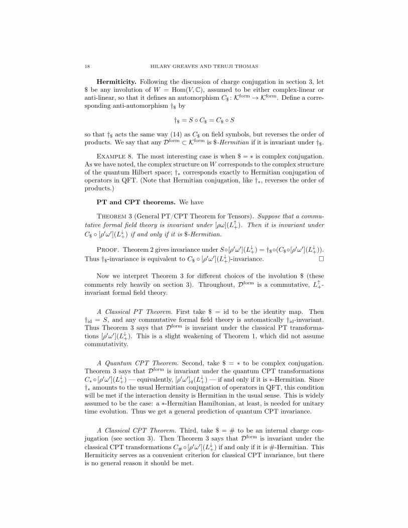
Hermiticity. Following the discussion of charge conjugation in section 3, let$ be any involution of W = Hom(V,C), assumed to be either complex-linear oranti-linear, so that it defines an automorphism C$ : Kform → Kform. Define a corre-sponding anti-automorphism †$ by

†$ = S ◦ C$ = C$ ◦ S

so that †$ acts the same way (14) as C$ on field symbols, but reverses the order ofproducts. We say that any Dform ⊂ Kform is $-Hermitian if it is invariant under †$.

Example 8. The most interesting case is when $ = ∗ is complex conjugation.As we have noted, the complex structure onW corresponds to the complex structureof the quantum Hilbert space; †∗ corresponds exactly to Hermitian conjugation ofoperators in QFT. (Note that Hermitian conjugation, like †∗, reverses the order ofproducts.)

PT and CPT theorems. We have

Theorem 3 (General PT/CPT Theorem for Tensors). Suppose that a commu-tative formal field theory is invariant under [ρω](L↑+). Then it is invariant underC$ ◦ [ρ′ω′](L↓+) if and only if it is $-Hermitian.

Proof. Theorem 2 gives invariance under S◦[ρ′ω′](L↓+) = †$◦(C$◦[ρ′ω′](L↓+)).Thus †$-invariance is equivalent to C$ ◦ [ρ′ω′](L↓+)-invariance. �

Now we interpret Theorem 3 for different choices of the involution $ (thesecomments rely heavily on section 3). Throughout, Dform is a commutative, L↑+-invariant formal field theory.

A Classical PT Theorem. First take $ = id to be the identity map. Then†id = S, and any commutative formal field theory is automatically †id-invariant.Thus Theorem 3 says that Dform is invariant under the classical PT transforma-tions [ρ′ω′](L↓+). This is a slight weakening of Theorem 1, which did not assumecommutativity.

A Quantum CPT Theorem. Second, take $ = ∗ to be complex conjugation.Theorem 3 says that Dform is invariant under the quantum CPT transformationsC∗ ◦ [ρ′ω′](L↓+) — equivalently, [ρ′ω′]q(L

↓+) — if and only if it is ∗-Hermitian. Since

†∗ amounts to the usual Hermitian conjugation of operators in QFT, this conditionwill be met if the interaction density is Hermitian in the usual sense. This is widelyassumed to be the case: a ∗-Hermitian Hamiltonian, at least, is needed for unitarytime evolution. Thus we get a general prediction of quantum CPT invariance.

A Classical CPT Theorem. Third, take $ = # to be an internal charge con-jugation (see section 3). Then Theorem 3 says that Dform is invariant under theclassical CPT transformations C# ◦ [ρ′ω′](L↓+) if and only if it is #-Hermitian. ThisHermiticity serves as a convenient criterion for classical CPT invariance, but thereis no general reason it should be met.

THE CPT THEOREM 19

A Quantum PT Theorem. Finally, define $(λ)(v) = λ(#v)∗ for some internalcharge conjugation #; we write ‘$ = ∗#.’ Theorem 3 now says that Dform isinvariant under the quantum PT transformations C∗# ◦ [ρ′ω′](L↓+) — equvialently,C#◦[ρ′ω′]q(L↓+) — if and only if it is ∗#-Hermitian. There is again no general reasonthis condition should be met. Note this result does not assume that the theory isHermitian in the usual sense, i.e. ∗-Hermitian. However, when, as usual, Dform

is ∗-Hermitian, being ∗#-Hermitian is equivalent to being C#-invariant. In otherwords, we have the usual implication of the CPT theorem, that charge-conjugationinvariance is equivalent to PT invariance.

Remark. The commutativity assumption is required for the results in thissection, though it plays no role in Theorem 1. We could not instead assume anti-commutativity, because an anti-commutative formal field theory would not be in-variant under S. As a trivial example, consider the complex scalar field of Example4. The formula F = ΦλΦλ

∗+ 1 is ∗-Hermitian and L↑+-invariant, but under quan-

tum CPT transforms to Φλ∗Φλ + 1. If Φλ and Φλ

∗commute, then this is just F

again; but if they anti-commute, it equals −F + 2, and F is not CPT invariant.

7. Covers of the Lorentz Group

We now begin to generalise our results to spinors, as explained in section 4.3.The purpose of this section is to describe the covering groups of L+, and, in particu-lar, to construct the covering group bL+ mentioned in our Quantum CPT Theorem.

We continue to assume that the dimension of Minkowski space M is at leastthree. At the end we work out an explicit description of all the groups in thefour-dimensional case (Example 9).

Covering groups of L+(C). It is convenient to start our discussion withcovering groups of the complex proper Lorentz group. L+(C) is connected, butnot simply connected. Since it is connected, it has a universal cover L+(C)∧; sinceit is not simply connected, L+(C)∧ is not just equal to L+(C). In fact L+(C)∧

is a double cover. For future reference, it is convenient to state this directly asa property of L↑+, using the fact (Lemma 5.1) that L+(C) is the complexification(L↑+)C of L↑+:

(PT-4) The universal cover π : ((L↑+)C)∧ → (L↑+)C is a double cover.We now use this double cover to define a four-fold cover π : L+(C)→ L+(C).

Definition 7. Let {1, τ} ⊂ L+(C)∧ be the preimage of 1 ∈ L+(C). Let L+(C)be the group generated by L+(C)∧ together with a symbol I such that I2 = τ , andsuch that I commutes with elements of L+(C)∧. Defining π(I) = 1, we obtain afour-fold covering map π : L+(C)→ L+(C).

The situation is illustrated in Figure 1 (with further details explained below).

Covering groups of L+. Let L↑+ be the preimage of L↑+ in L+(C)∧. This isa double cover of L↑+; in fact it is the universal cover (except when dimM = 3; seeRemark 7.1). We similarly define two different double-covers of L+, illustrated inFigure 1. First, let aL+ = L↑+ ∪ aL

↓+, where aL

↓+ is the preimage of L↓+ in L+(C)∧.

Second, let bL+ = L↑+ ∪ bL↓+, where bL

↓+ = I · aL↓+. It can be shown that any double

cover of L+ containing L↑+ is isomorphic to either aL+ or bL+ (we omit the proof).


& %L+(C)� �L↑+� � L↓+

?

'&

$%L+(C)∧

��

'&

$%

��

-

-��τ-

-��τ

�

��

�I : I2 = τ

π

L↑+aL↓+

bL↓+IL↑+

IL+(C)∧

Figure 1. A four-fold cover L+(C) of the complex proper Lorentzgroup L+(C), with two components. It contains the two doublecovers of L+ extending L↑+: aL+ = L↑+ ∪ aL

↓+ and bL+ = L↑+ ∪ bL

↓+.

Example 9. In four dimensions we have L↑+ ∼= SL(2,C), the group of 2 × 2matrices with complex entries and unit determinant. It is important to bear inmind that, despite notation, L↑+ is only a real Lie group; it has no natural com-plex structure. The covering map π : SL(2,C) → L↑+ can be specified as follows.Arbitrarily choosing an inertial coordinate system, we can identify L↑+ with a sub-group of GL(4,R). Hence, to specify a covering map, it suffices to specify anaction π of SL(2,C) on R4 preserving the Minkowski norm x2

0 − x21 − x2

2 − x33. For

x = (x0, x1, x2, x3) ∈ R4, write

(16) 〈x〉 =

(x0 + x3 x1 − ix2

x1 + ix2 x0 − x3

);

then, the desired action of A ∈ SL(2,C) is given by the matrix multiplication

(17) 〈π(A)(x)〉 = A · 〈x〉 · AT

(here A is the complex-conjugate of A, and T denotes transpose). The Minkowskinorm of x is equal to det 〈x〉, which is preserved under (17) since detA = det AT =1. Note that π is two-to-one: π(A) = π(−A) for all A ∈ SL(2,C).

The universal cover L+(C)∧ of L+(C) is isomorphic to SL(2,C)×SL(2,C). Thecovering map is defined as follows. For x ∈ MC = C4, define 〈x〉 as in (16). For(A,B) ∈ SL(2,C)× SL(2,C), π(A,B) is the linear transformation of C4 given by

(18) 〈π(A,B)(x)〉 = A · 〈x〉 ·BT .

Thus L↑+ is identified with the subgroup of pairs (A, A), and τ is represented bythe pair (−1,−1) of scalar matrices. To describe the four-fold cover L+(C), werepresent I by the pair (i,−i) of scalar matrices. This brings us to the following

THE CPT THEOREM 21

picture, where H is the group of 2× 2 complex matrices with determinant ±1.

L+(C) ∼= {(A,B) ∈ H ×H | detA = detB}L+(C)∧ ∼= {(A,B) ∈ H ×H | detA = detB = 1}

L↑+∼= {(A, A) ∈ H ×H | detA = 1}

aL↓+∼= {(A,−A) ∈ H ×H | detA = 1}

bL↓+∼= {(A,−A) ∈ H ×H | detA = −1}.

The covering map π : L+(C) → L+(C) is still given by (18). It is four-to-one: forall (A,B) ∈ L+(C), π(A,B) = π(−A,−B) = π(iA,−iB) = π(−iA, iB).

Remark 7.1. If dimM = 3, then L↑+ is not the universal cover (L↑+)∧ (whichturns out to be an infinite cover of L↑+). However, it is still true that any projec-tive representation of L↑+ comes from a representation of L↑+, so there is no lossof generality in considering L↑+ rather than (L↑+)∧. Note that any representationof L↑+ determines a representation of (L↑+)∧, by composing with the covering map(L↑+)∧ → L↑+. The claim is that every representation of (L↑+)∧ arises in this way.One can check that the map (L↑+)∧ → L↑+ ⊂ L+(C)∧ identifies L+(C)∧ with thecomplexification of (L↑+)∧ (compare to Lemma 8.1). This means that any repre-sentation ρ of (L↑+)∧ on V extends to a representation ρC of L+(C)∧ on V C, andtherefore ρ(g) depends only on the image of g in L↑+.

8. A Classical PT Theorem for Spinor Fields?

Having described the covering groups of L+, we now naively attempt to gener-alise Theorem 1 to the case of spinors. In fact, we will fail in this attempt, but theargument will lead to a generalisation of Theorems 2 and 3 in the next section.

Following the exposition in section 5, we can complexify any representation(ρ, L↑+, V ) to get (ρC, (L↑+)C, V C). Next, we wish to restrict ρC to either aL+ or bL+.In analogy to Lemma 5.1, we have

Lemma 8.1. The inclusion L↑+ → L+(C)∧ identifies L+(C)∧ with the complex-ification (L↑+)C. In particular, aL+ is a subgroup of (L↑+)C.

The proof is in Appendix C. The result is that we can restrict ρC to a repre-sentation of aL+ (but not of bL+) on V C. However, this does not mean that aL+

preserves V ⊂ V C, and, in fact, the analogue of Lemma 5.2 fails; rather, one has

Lemma 8.2. Let (ρ, L↑+, V ) be a representation of L↑+, and (ρC, (L↑+)C, V C) itscomplexification. Decompose V as V = V0 ⊕ V1 where ρ(τ) acts as (−1)n on Vn.Then ρC(aL↓+) preserves V0 but maps V1 to iV1 ⊂ V C.

Since ρC(aL↓+) does not preserve all of V ⊂ V C, there is no obvious way todefine a representation of aL+ on V , and therefore no obvious way to associate PTtransformations to elements of aL↓+.

Remark. A representation V0 on which τ acts by the identity is the same thingas a representation of L↑+. Thus we can speak of V0 as the space of ‘tensors’ and


V1 as the space of ‘pure spinors.’ When V = V0, V is preserved by aL↓+, and we doget a PT theorem – namely, Theorem 1.

Remark. Just as Lemma 5.2 relied on property (PT-3), so the proof of Lemma8.2 in Appendix C reduces to the following fact:

(PT-5) For any g ∈ aL↓+, g∗ = gτ .

It is automatic from (PT-1)–(PT-4) and the fact that L↓+ is connected, that either(PT-5) holds or else g∗ = g for all g ∈ aL↓+. In the latter case, we would haveobtained a classical PT theorem in analogy to Theorem 1.

Example 10. We continue Example 9. Let ρ be the standard representation ofL↑+ = SL(2,C) on C2. The complexity of V is completely irrelevant (cf. Example4), so to avoid confusion, let us write V = R4. For v = (x, y, z, w) ∈ V define[v] = (x+ iy, z + iw, x− iy, z − iw) ∈ C4. Then ρ is given by

[ρ(A)v] =

(A 00 A

)· [v].

Since τ is represented by A = −1, we find V = V1. The complexification of V = R4

is V C = C4. For v ∈ V C, define [v] ∈ C4 as before. Then the complexifiedrepresentation ρC of (L↑+)C = L+(C)∧ = SL(2,C)× SL(2,C) on V C is given by

[ρC(A,B)v] =

(A 00 B

)· [v].

Following Example 9, aL↓+ consists of pairs (A,−A). In particular, one finds that(1,−1) ∈ aL↓+ acts on V C by

ρC(1,−1)(x, y, z, w) = (iy,−ix, iw,−iz).

As predicted by Lemma 8.2, this maps real vectors into purely imaginary ones.

A Holomorphic Spinorial PT Theorem. As consolation, there is a classof field theories for which we can define a geometric action of aL+ and prove a PTinvariance theorem. We will sketch the idea here, but this discussion is merely anaside, and is not used in the rest of the paper.

Suppose that our representation (ρ, L↑+, V ) is complex in the sense that V isa complex vector space and L↑+ acts complex-linearly. This is already enough todefine a geometric action of aL+: there is a unique extension of ρ to a holomorphicrepresentation (ρhol, (L↑+)C, V ), and, in particular, an action of aL+ on V .

However, we will only get aL+-invariance for certain special field theories. Hereis one class of them. LetW+ ⊂W be the subspace of complex-linear maps V → C,and Kform

+ = F(W+ ⊗R TM) the free complex algebra generated by W+ ⊗R TM .This is a subalgebra of Kform, and it is invariant under the classical action of L↑+.We call a formal field theory Dform ⊂ Kform holomorphic if it is contained in Kform

+ .The following theorem is closely parallel to Theorem 1; we omit its proof.

Theorem 4. If a holomorphic formal field theory is invariant under [ρω](L↑+),then it is invariant under [ρholω′](aL↓+).

However, most theories of physical interest are not ‘holomorphic’ in this sense.If the original representation ρ is not complex (e.g. the case of Majorana spinors),

THE CPT THEOREM 23

then Lemma 8.1 tells us that aL↓+ takes fields with values in V1 to fields with valuesin iV1 – i.e., outside the original space of kinematically allowed fields. Similarly,if the original representation ρ is complex but the dynamics cannot be describedby a subspace of Kform

+ , then aL↓+ preserves the kinematical space, but not thedynamical subspace. Theorem 4 therefore does not yield an invariance theorem forfield theories that are ‘non-holomorphic’ in either of these two ways.

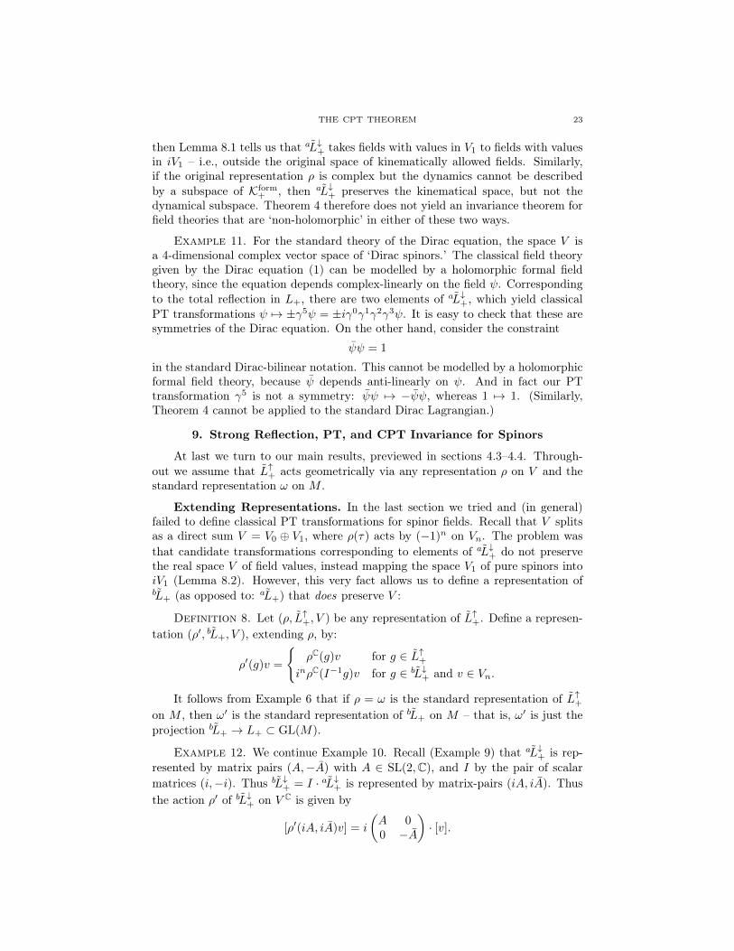
Example 11. For the standard theory of the Dirac equation, the space V isa 4-dimensional complex vector space of ‘Dirac spinors.’ The classical field theorygiven by the Dirac equation (1) can be modelled by a holomorphic formal fieldtheory, since the equation depends complex-linearly on the field ψ. Correspondingto the total reflection in L+, there are two elements of aL↓+, which yield classicalPT transformations ψ 7→ ±γ5ψ = ±iγ0γ1γ2γ3ψ. It is easy to check that these aresymmetries of the Dirac equation. On the other hand, consider the constraint

ψψ = 1

in the standard Dirac-bilinear notation. This cannot be modelled by a holomorphicformal field theory, because ψ depends anti-linearly on ψ. And in fact our PTtransformation γ5 is not a symmetry: ψψ 7→ −ψψ, whereas 1 7→ 1. (Similarly,Theorem 4 cannot be applied to the standard Dirac Lagrangian.)

9. Strong Reflection, PT, and CPT Invariance for Spinors

At last we turn to our main results, previewed in sections 4.3–4.4. Through-out we assume that L↑+ acts geometrically via any representation ρ on V and thestandard representation ω on M .

Extending Representations. In the last section we tried and (in general)failed to define classical PT transformations for spinor fields. Recall that V splitsas a direct sum V = V0 ⊕ V1, where ρ(τ) acts by (−1)n on Vn. The problem wasthat candidate transformations corresponding to elements of aL↓+ do not preservethe real space V of field values, instead mapping the space V1 of pure spinors intoiV1 (Lemma 8.2). However, this very fact allows us to define a representation ofbL+ (as opposed to: aL+) that does preserve V :

Definition 8. Let (ρ, L↑+, V ) be any representation of L↑+. Define a represen-tation (ρ′, bL+, V ), extending ρ, by:

ρ′(g)v =

{ρC(g)v for g ∈ L↑+

inρC(I−1g)v for g ∈ bL↓+ and v ∈ Vn.

It follows from Example 6 that if ρ = ω is the standard representation of L↑+on M , then ω′ is the standard representation of bL+ on M – that is, ω′ is just theprojection bL+ → L+ ⊂ GL(M).

Example 12. We continue Example 10. Recall (Example 9) that aL↓+ is rep-resented by matrix pairs (A,−A) with A ∈ SL(2,C), and I by the pair of scalarmatrices (i,−i). Thus bL↓+ = I · aL↓+ is represented by matrix-pairs (iA, iA). Thusthe action ρ′ of bL↓+ on V C is given by

[ρ′(iA, iA)v] = i

(A 00 −A

)· [v].


In particular, one finds that (i, i) ∈ bL↓+, corresponding to a total reflection of M ,acts on V by ρ′(i, i)(x, y, z, w) = (−y, x,−w, z).

Having shown how to extend geometric actions of L↑+ to bL+, we can at leastformulate analogues of Theorems 1 and 2. However, one cannot expect a directgeneralisation of Theorem 1 actually to hold, because ρ′ is not merely a restrictionof the complexification of ρ. It turns out that we can nonetheless get a directgeneralisation of Theorem 2, with the assumption of commutativity replaced bysupercommutativity, which we now explain.

Supercommutativity. If V = V0, then supercommutativity is just commu-tativity, as in section 6. If V = V1, we impose instead anti-commutativity,

Φλξ1···ξmΦµη1···ηn = −Φµη1···ηnΦλξ1···ξm .

In general, the decomposition V = V0⊕V1 leads to a decompositionW = W0⊕W1,where Wn = Hom(Vn,C). Then supercommutativity means that

(19) Φλξ1···ξmΦµη1···ηn = (−1)abΦµη1···ηnΦλξ1···ξm

holds for all λ ∈ Wa and µ ∈ Wb. The relations (19) define the free supercommu-tative algebra Kform

s = Fs(W ⊗R TM) (A.7 and A.8). Thus we can define a super-commutative formal field theory to be a complex affine subspace Dform ⊂ Kform

s .As with commutative theories, we can consider a supercommutative formal fieldtheory to be a special kind of formal field theory in the original sense, using themap Kform → Kform

s that conflates all formulae related by supercommutation (19).Supercommutativity is our version of the full spin-statistics connection.18 It

has a natural interpretation, and independent motivation via the spin-statisticstheorem, in the quantum case. In contrast, our discussion of classical field theoriesin section 2 leads to purely commutative rather than supercommutative formal fieldtheories, since the derived components of classical fields commute. Nonetheless, itis possible to make some sense of supercommutative classical spinorial field the-ories. First a trivial but important example: field theories determined by lineardynamical equations can be modelled in this way (see Remark 9.1 below). In theabsence of further compelling examples, we only sketch one general approach, whichmirrors the non-commutativity of quantum fields. Suppose that A = A0 ⊕A1 is a

18 There are several closely related statements that can be called ‘the spin-statistics connection.’In our approach, we formalize it by taking the theory-specifying differential formulae to livein the supercommutative algebra Kform

s . This agrees with the functional-integral approach toQFT, in which the Lagrangian density is interpreted by means of Grassmann-valued fields, whichsupercommute exactly as we have described.

From another point of view, however, our approach may seem to involve a false premiss. If weare to interpret the field symbols Φλξ1···ξn as fields, then, on the face of it, we seem to claim thatthe values of these fields at any given point commute or anti-commute. This is of course falseof the operator-valued fields of QFT, where commutators (or anti-commutators) vanish only atspace-like separations. The key to resolving this apparent contradiction is to remember that onecannot simply multiply together quantum field components at a single point: such products arenot usually well defined. One must regularize these products in some way, and whatever method isused should ultimately reproduce the supercommutativity seen in the functional integral approach.For example, in the interaction picture of section 2.4, the interaction density is not simply a sumof products of free quantum fields and their spacetime derivatives, but, rather, the normal-orderedcounterpart of such an expression. And field operators do strictly supercommute within normal-ordered expressions.

THE CPT THEOREM 25

supercommutative algebra; let K = C∞(M,A0⊗R V0⊕A1⊗V1). Then the derivedcomponents of any Φ ∈ K are functions with values in AC, and thus supercommute.

Invariance. We arrive at our main results:

Theorem 5 (Strong Reflection Invariance). If a supercommutative formal fieldtheory is invariant under [ρω](L↑+), then it is invariant under S ◦ [ρ′ω′](bL↓+).

Strong reflection invariance entails PT and CPT theorems, by the same argu-ments as in section 6. To spell things out, we consider, as in section 6, an arbitrarycomplex-linear or anti-linear involution $ of W , and we extend this to an automor-phism C$ and an anti-automorphism †$ of Kform. Then it is easy to deduce

Theorem 6 (General PT/CPT Theorem). Suppose that a supercommutativeformal field theory is invariant under [ρω](L↑+). Then it is invariant under C$ ◦[ρ′ω′](bL↓+) if and only if it is $-Hermitian.

Note that Theorems 5 and 6 subsume Theorems 2 and 3, which correspondto the the special case V = V0. The proof of Theorem 5 is in Appendix C. Thededuction of Theorem 6 from Theorem 5 is completely parallel to the deduction ofTheorem 3 from Theorem 2.

PT and CPT. The same argument as in section 5 shows that if [ρω](L↑+) ischarge-preserving, then [ρ′ω′](bL↓+) is too. To spell it out: since each sector W ε ⊂Kforms is assumed [ρω](L↑+)-invariant, it is S ◦ [ρ′ω′](bL↓+)-invariant, by Theorem 5;

but it is obviously S invariant, so it must be [ρ′ω′](bL↓+)-invariant. Thus [ρ′ω′](bL↓+)is charge-preserving, as claimed.

As in section 6, a quantum CPT theorem is recovered from Theorem 6 bysetting $ = ∗; for $ = id,#, ∗# we obtain, respectively, a classical PT theorem, aclassical CPT theorem, and a quantum PT theorem. The quantum CPT theoremis the most important of these: it is the CPT theorem of Lagrangian QFT, in whichits premisses (supercommutativity and ∗-Hermiticity) are widely accepted.

Example 13. Again the particular spin-statistics connection that we have as-sumed is indeed required for Theorem 6. Suppose instead we assumed that spinorscommute with one another. Consider the equation

(20) ψψ = 1,

where ψ is a Dirac spinor field (cf. Example 11). The total reflection in L+

corresponds to two elements of bL↓+, which act on ψ by ψ 7→ ±iγ5ψ under [ρ′ω′].But if spinors commute then under the CPT transformation ψ 7→ (iγ5ψ)∗ we haveψψ 7→ −ψψ (cf. the appeal to fermion anti-commutation in equation (3.147) of(Peskin & Schroeder, 1995)). Hence, (20) transforms to −ψψ = 1, which is actuallyincompatible with (20).

Remark 9.1. The classical PT theorem of section 6 applied only to commu-tative tensor fields, for which the requirement of id-Hermiticity is trivial. It is nolonger trivial for spinor fields, although it holds for a wider class than merely tensorfields. For example, suppose that a classical spinorial field theory D is specified bylinear differential formulae, like the free Dirac equation. The span Dform ⊂ Kform

s

of those linear formulae is an id-Hermitian, supercommutative formal field theory,and its classical spacetime symmetries correspond exactly to spacetime symmetries


of D. Thus if D is L↑+-invariant, so is Dform, and our present classical PT theorempredicts PT invariance. Note that in this case, we have made Dform supercommu-tative in order to apply the theorem, but this supercommutativity is irrelevant tothe interpretation of Dform as a classical field theory: for linear equations, thereis no substantial question of commutativity or supercommutativity, since there areno products to commute or supercommute.

9.1. Symmetries of free quantum theories. Following the discussion insection 2.4, it is useful to explain separately how Theorem 6 yields symmetriesof free quantum field theories. Recall that the free theory is specified by a qua-dratic Lagrangian density, giving rise to linear field equations. The Hilbert spaceis related by a Fock space construction to the classical theory defined by these lin-ear equations. As explained in (?, ?), the construction is such that classical andquantum L↑+-invariance are equivalent, and classical PT invariance is equivalent toquantum CPT invariance. So we can argue as follows. If the free quantum theoryis L↑+-invariant, so is the classical theory. Our classical PT theorem (which appliesby Remark 9.1) then predicts classical PT invariance, which implies quantum CPTinvariance. (The hypothesis that the Lagrangian density is Hermitian is implicitin this story. For one thing, it guarantees that there are enough solutions to theclassical field equations. It is also used to define the inner product on the Hilbertspace.)

A similar argument establishes that a free QFT is PT invariant if the freeLagrangian density is ∗#-Hermitian. This Hermiticity implies that the system oflinear field equations is ∗#-Hermitian as well. Now, classical field equations canalways be written using only real coefficients (cf. the discussion around (1)). Thisshows that the system of field equations is C∗-invariant, hence #-Hermitian, hence,by Theorem 6, classically CPT invariant. And this implies that the free QFT isPT invariant.

10. Other Spacetimes, Other Groups

Our theorems apply in principle to other spacetimes besides Minkowski space,and to other groups besides the Lorentz group. Any group L+ = L↑+∪L

↓+ will satisfy

‘tensorial’ invariance theorems like Theorems 1–3 as long as it satisfies conditions(PT-1)–(PT-3) of section 5. We will obtain ‘spinorial’ invariance theorems likeTheorems 5–6 if L+ also satisfies (PT-4) of section 7 and (PT-5) of section 8.

In this section we consider one setting to which our results extend, and several towhich they don’t. Of course, we have not shown that properties (PT-1)–(PT-3) arenecessary for any invariance theorem to hold. However, in cases where these axiomsfail, we have no general grounds to expect invariance theorems, and understandinghow they fail provides a conceptual complement to ad hoc counterexamples.

General Non-Euclidean Signatures. Let M be a vector space with anynon-Euclidean inner product (i.e. at least one ‘timelike’ and one ‘spacelike’ di-mension), and dimM ≥ 3. Let L+ be the group of linear isometries of M withdeterminant +1. Then L+ = L↑+ ∪ L

↓+ has two components, and satisfies (PT-

1)–(PT-5); our constructions and Theorems 1–6 work without change. However,there are two conceptual points to make. First, L↓+ consists of transformations thatreverse parity and the orientation of time. We must understand ‘time-reversing’in Definition 3 in this sense. Note that it is possible for some timelike vectors to

THE CPT THEOREM 27

be reversed but others fixed: for example, with two timelike and one spacelike di-rection, (t1, t2, x) 7→ (t1,−t2,−x) defines an element of L↓+ that fixes the timelikevector (1, 0, 0). The second point is that the preimage L↑+ of L↑+ in L+(C)∧ maynot be the universal cover of L↑+. However, as in Remark 7.1, there is no loss ofgenerality in using L↑+ instead of (L↑+)∧.

No CPT Theorem in Dimension 2. Let M be two-dimensional Minkowskispace. Then L+ = L↑+ ∪ L

↓+ satisfies (PT-1) but not (PT-2) or (PT-3). In fact, if

g ∈ (L↑+)C is fixed by complex conjugation, then g ∈ L↑+. This is closely relatedto the failure of (PT-4): the universal cover of (L↑+)C is an infinite cover. Thus wedo not expect any PT or CPT theorem; the following example shows that therecannot be one.

Example 14. Choose a null-vector ξ ∈ M . Then for each g ∈ L↑+ there issome j(g) ∈ R such that g · ξ = ej(g)ξ. This gives an isomorphism j : L↑+ → R. Let(ρ, L↑+, V ) be the one-dimensional representation of L↑+ given by V = R, ρ(g)v =

ej(g)/4v. Consider the classical field theory given by the single dynamical equation

Φ3∂ξΦ = 1.

It is easy to check that this equation is L↑+-invariant. However, if there is a PT(or CPT) transformation, it must act on V by some scalar α ∈ R, and transform∂ξ 7→ −∂ξ. Then it transforms our dynamical equation by Φ3∂ξΦ 7→ −α4Φ3∂ξΦ.Our theory will only be PT invariant if α4 = −1; this is impossible since α is real.Nor can we salvage the situation by the use of anti-commuting fields.

No P or T Theorems. If in Minkowski space we consider L↑+ ∪ L↑− or L↑+ ∪

L↓−, then condition (PT-2) fails to hold: the only conjugation-fixed elements of(L↑+)C are elements of L+. Thus we do not expect invariance under (C)P or (C)Ttransformations, and it is well known that such symmetries fail to exist in somephysical examples.

No Galilean Theorems. Let M be a Galilean spacetime of dimension d,with a fixed origin. In detail, the data is a quadruple (M,Ms, ηs, ηt), where Mis a vector space, Ms ⊂ M is a hyperplane, ηs is a Euclidean metric on ‘space’Ms, and ηt is a Euclidean metric on ‘time’ M/Ms. As in Minkowski space, theautomorphism group L of (M,Ms, ηs, ηt) has four components, L↑+∪L

↑−∪L

↓−∪L

↓+.

In this case, the only conjugation-fixed elements of (L↑+)C lie in L↑+ itself. Thus wedo not expect general (C)PT, (C)T, or (C)P theorems in Galilean spacetime; thefollowing example shows that there cannot be one.

Example 15. Consider fields taking values in V = R, with the trivial action ofL↑+. Choose a basis ξ0, ξ1, . . . , ξd−1 forM with ξ1, . . . ξd−1 ∈Ms. Then the classicalfield theory given by the differential equations

∂ξ0Φ = Φ ∂ξ1Φ = · · · = ∂ξd−1Φ = 0

is L↑+-invariant but cannot be invariant under any transformation that reversestime. In particular, this rules out PT and CPT theorems.


11. Conclusions

The CPT theorem follows from the following assumptions:(1) The theory is specified by polynomials in the fields and their spacetime

derivatives, i.e. by a formal field theory Dform.(2) Dform is invariant under a classical/quantum action of the proper or-

thochronous Lorentz group, or of a covering group (the classical and quan-tum actions being equivalent for the orthochronous group).

(3) The spin-statistics connection holds (in that Dform is supercommutative).(4) Dform is invariant under Hermitian conjugation.

These four assumptions lead to the CPT invariance of Dform; there is a furtherinterpretive assumption that this implies the CPT invariance of the underlying(non-formal) theory.

We are not aware of any way of substantially weakening these assumptions whileretaining the CPT result. There are two partial exceptions. First, it is possibleto treat some non-polynomial theories (see Example 2). Second, one can replacethe proper Lorentz group by any group satisfying our axioms (PT-1)–(PT-5) (seesection 10).

The proof of the CPT theorem given in the present paper differs from thosein Lagrangian QFT texts primarily in its completeness and its reliance on basicgeometric facts. The usual approach works only in 3+1 spacetime dimensions, andtypically restricts consideration to scalars, vectors, and Dirac spinors. It introducesapparently ad hoc C, P, and T transformations in these cases, and establishes CPTinvariance by computing its effects on an exhaustive list of sixteen ‘Dirac bilinears.’These calculations are then (if ever) generalised by appealing to a detailed classi-fication of representations of the four-dimensional Lorentz group. In contrast, weuse the general notion of complexification to define and study canonical CPT trans-formations, at no point appealing to exhaustive classifications. As a consequence,our proof applies at once to representations of higher spin, and to Weyl as well asDirac spinors for the case of spin 1

2 . It also applies in any spacetime that sharesthe essential group-theoretic facts: it works for Minkowski space and, with onlyminor modifications, for any non-Euclidean signature in dimension at least 3. Ourapproach also differs from the axiomatic treatments of e.g. Streater and Wightmanin that it applies directly to the the kind of Lagrangian quantum field theories thatenjoy empirical success.

Our proof of the quantum CPT theorem also establishes quantum PT, classicalPT and classical CPT theorems. All are equally theorems; the reason for regardingthe quantum CPT result as the most interesting of the four is (‘only’) that therequired supercommutativity assumption has independent motivation in the quan-tum but not in the classical case, while the required Hermiticity assumption hasindependent motivation in the quantum CPT but not in the quantum PT case.

Appendix A. Mathematical Background

In this appendix we recall the mathematical background used in the main text.The aim is to point out the important ideas, rather than to provide a detailedexposition. In doing so, we fix some useful terminology and notation.

I. Representations and Algebras

THE CPT THEOREM 29

A.1. Vector Spaces. All vector spaces we consider will be real, and all mapsbetween vector spaces are real-linear. We also consider complex vector spaces, whichmay be considered as real ones with additional structure. If V, V ′ are complex vectorspaces, then a (real-linear) map f : V → V ′ is complex-linear if f(iv) = if(v) forall v ∈ V , and anti-linear if f(iv) = −if(v) for al v ∈ V .

A complex subspace of a complex vector space V is a subset closed under addi-tion and multiplication by complex numbers. In contrast, a complex affine subspaceW ⊂ V is a subset such that if x, y ∈ W and a ∈ C then ax + (1 − a)y ∈ W . Acomplex affine subspace is a complex subspace if and only if it contains 0 ∈ V .

A.2. Lie groups. A Lie group is a manifold G that is also a group, for whichthe multiplication and inversion maps are smooth. Homomorphisms between Liegroups are required to be smooth.

Example 16. For any finite-dimensional vector space V , the group GL(V ) of(real-linear) automorphisms of V is naturally a Lie group. It has two connectedcomponents. The component GL+(V ) containing the identity consists of thoselinear maps with positive determinants.

A Lie group is ‘complex’ if it is in fact a holomorphic manifold, and the multi-plication and inversion maps are holomorphic. A homomorphism between complexLie groups may or may not be holomorphic in the usual sense for maps betweenholomorphic manifolds.

Example 17. IfW is a finite-dimensional complex vector space, then the groupGLC(W ) of complex-linear automorphisms is a complex Lie group.

A.2.1. Covering Groups. A homomorphism G′ → G of Lie groups is a cov-ering map if it is surjective and a local diffeomorphism; we say that G′ is a coveringgroup or simply a cover of G. A covering π : G′ → G is trivial if there is a section,i.e. a homomorphism s : G → G′ such that π ◦ s is the identity map. If G′ isconnected, then π is trivial if and only if it is an isomorphism.

Covering groups have a path lifting property. The case we need is that anyhomomorphism R→ G of Lie groups lifts uniquely to a homomorphism R→ G′.

If G is connected, then it has a unique universal cover G∧. The coveringmap πG : G∧ → G is uniquely characterised by the following property: for anycovering map α : G′ → G, with G′ connected, there exists a unique covering mapπG′ : G

∧ → G′ such that πG = α ◦ πG′ . It follows that this πG′ is the universalcovering map for G′. It also follows that if π : G′ → G∧ is a covering map, andG′ is connected, then π is an isomorphism. (Indeed, πG ◦ π : G′ → G is a coveringmap, so we obtain a covering map πG′ : G∧ → G′, which must be inverse to π.)

A.2.2. Lie Algebras. Given a Lie group G, let Lie(G) denote the tangentspace to G at the identity. If G is a complex Lie group, then Lie(G) is a complexvector space. A homomorphism α : G→ H induces a linear map Lie(α) : Lie(G)→Lie(H) (the derivative of α at the identity); if G is connected, α is completelydetermined by Lie(α). If G and H are connected, then α is a covering map if andonly if Lie(α) is an isomorphism.

Example 18. For any finite-dimensional vector space V , Lie(GL(V )) is thevector space of all linear maps f : V → V . For L↑+ ⊂ GL(M), one can show that


Lie(G) ⊂ Lie(GL(M)) consists of those f such that

η(f(v), w) + η(v, f(w)) = 0 for all v, w ∈M.

If V is complex, then Lie(GLC(V )) is the space of all complex -linear maps V → V .

A.3. Representations. All representations in this paper are either finite di-mensional or what we call quasi-finite. A finite-dimensional representation of aLie group is a triple (ρ,G, V ), where V is a finite-dimensional vector space, G is aLie group, and ρ : G → GL(V ) is a homomorphism of Lie groups. Often we speakof ‘the representation (or action) ρ of G on V .’ A representation is holomorphicif V is a complex vector space, G a complex Lie group, and ρ is a holomorphichomomorphism.

A.3.1. Quasi-finite Representations. We also consider certain infinite-dimen-sional representations (ρ,G, V ). Again V is a vector space and ρ is a homomorphismG → GL(V ). But there is a technicality here in that if V is infinite dimensional,then GL(V ) is not a Lie group in the usual sense. However, all representationsthat we consider are quasi-finite in the following sense: there is a sequence offinite-dimensional subspaces V 1 ⊂ V 2 ⊂ · · · such that the union is V , each V n isρ(G)-invariant, and the resulting homomorphisms ρn : G → GL(V n) are smooth.These conditions allow us to apply notions that are initially valid only for finitedimensional representations. For example, a quasi-finite representation is ‘holo-morphic’ if every ρn is holomorphic. We will use this technical device withoutfurther comment.

A.4. Algebras. An algebra is a real vector space A with a bilinear, associa-tive, unital multiplication A ⊗R A → A. A homomorphism of algebras is a linearmap preserving the multiplication and the unit. An algebra is complex if A is acomplex vector space, and the multiplication is complex-bilinear. A (real-linear)homomorphism f between complex algebras may be complex-linear or anti-linear.

A.5. Graded Vector Spaces and Algebras. A vector space V is Z-graded(or merely graded) if it is given as a direct sum

V =⊕n∈Z

Vn

of vector spaces Vn labelled by integers. An algebra is graded if it is a gradedvector-space and ab ∈ Am+n for all a ∈ Am, b ∈ An.

II. Free Algebras

A.6. Tensor Algebras. Suppose that V is a real vector space. The tensor(or free) algebra TV consists of formal sums of products of elements of V . Moreprecisely, if v1, . . . , vn is a basis for V , then TV consists of non-commutative poly-nomials in variables v1, . . . , vn, with real coefficients. More conceptually,

TV = R⊕ V ⊕ (V ⊗R V )⊕ (V ⊗R V ⊗R V )⊕ · · · =⊕n≥0

V ⊗n.

The key property of TV is that any real-linear map V → V extends uniquely to ahomomorphism TV → TV of algebras.

THE CPT THEOREM 31

A.7. Free Complex Algebras. The analogous construction for a complexvector space V is the free complex algebra F(V ) defined by

F(V ) = C⊕ V ⊕ (V ⊗C V )⊕ (V ⊗C V ⊗C V )⊕ · · · =⊕n≥0

V ⊗n.

If v1, . . . , vn is a complex basis for V , then F(V ) consists of non-commutativepolynomials in variables v1, . . . , vn, with complex coefficients. The key property isthat any complex-linear or anti-linear map V → V extends uniquely to a complex-linear or anti-linear homomorphism F(V )→ F(V ) of algebras.

A.8. Commutativity and Supercommutativity. The free commutativecomplex algebra Fc(V ) is constructed from F(V ) by imposing the relation

ab = ba ∈ Fc(V ) for all a, b ∈ V.

Thus elements of F(V ) that differ only by commutation are considered equal aselements of Fc(V ). Concretely, if v1, . . . , vn is a basis for V , then Fc(V ) is thealgebra of (usual, commutative) polynomials in variables v1, . . . , vn, with complexcoefficients.

If V is a graded complex vector space, then the free supercommutative complexalgebra Fsc(V ) is constructed from F(V ) by imposing the ‘supercommutativity’relations

ab = (−1)mnba for all a ∈ Vm, b ∈ Vn.For example, if V = V0 then Fsc(V ) = Fc(V ), and if V = V1 then Fsc(V ) isknown as the Grassmann or exterior algebra of V . If V is a graded vector space,then Fsc(V ) (like TV , F(V ), or Fc(V )) is naturally a graded algebra. Concretely,(Fsc(V ))m is spanned by products vd1 · · · vdn , with each vdk ∈ Vdk and

∑dk = m.

A.9. Extending Representations. As we have said, any complex-linear oranti-linear map V → V extends uniquely to a homomorphism F(V ) → F(V ) ofalgebras. In particular, suppose that (ρ,G, V ) is a representation such that eachtransformation ρ(g) is either complex-linear or anti-linear; then there is a uniquerepresentation (ρF , G,F(V )) such that each ρF (g) is an algebra automorphism.Explicitly: ρF (g) : F(V ) → F(V ) is the unique homomorphism of algebras ex-tending ρ(g) : V → V . One similarly obtains representations (ρFc , G,Fc(V )) and(ρFsc , G,Fsc(V )).

III. Complexification

A.10. Vector Spaces. Complexification is a universal way to replace realobjects by complex ones. For a real vector space V , its complexification V C is thetensor product

V C = C⊗R V := {a+ bi | a, b ∈ V }.It is characterised by the property that any real-linear map α : V → V ′ into acomplex vector space V ′ extends uniquely to a complex-linear map αhol : V C → V ′.In other words, the set of real-linear maps V → V ′ is naturally identified with theset of complex-linear maps V C → V ′.

Remark. If V is complex, then we can still form its complexification V C. Thisis not equal to V , unless of course V = 0. In general, if V has n real dimensions,then V C has 2n real dimensions.


A.11. Lie Groups. Given a connected Lie group G, its complexification GC

is a complex Lie group, equipped with a homomorphism i : G→ GC, characterisedby the following property: any homomorphism α : G→ G′ into a complex Lie groupG′ extends uniquely to a holomorphic homomorphism αhol : GC → G′. That is, αhol

uniquely satisfies αhol ◦ i = α.For the construction of GC, see (?, ?, Ch. 3, §6, Prop. 20). The essential fact

for us is that Lie(GC) = (LieG)C (the right-hand side being the complexificationin the sense of vector spaces).

Remark. Note that, in general, G may not be a subgroup of GC; there isonly a homomorphism between them. However, this homomorphism happens to beinjective in most cases of interest, and in particular for the Lorentz group.

Example 19. If V is a finite-dimensional real vector space, then GL+(V ) isa connected Lie group. If dimV > 1 then GL+(V )C = GLC(V C). However, ifdimV = 1 then GL+(V ) is isomorphic to the additive group of real numbers,and GL+(V )C to the additive group of complex numbers, whereas GLC(V C) isisomorphic to the multiplicative group of non-zero complex numbers.

A.12. Extending Representations. Consider a representation (ρ,G, V ) ofa connected Lie group G. If V is complex, and every ρ(g) is complex-linear, then(ρ,G, V ) extends uniquely to a holomorphic representation (ρhol, GC, V ). Namely,ρhol : GC → GLC(V ) is the unique holomorphic homomorphism extending ρ : G →GLC(V ). If V is not assumed to be complex, (ρ,G, V ) extends uniquely to aholomorphic representation (ρC, V C, GC) ofGC on V C. That is, ρC : GC → GLC(V C)is the unique holomorphic homomorphism extending ρ : G→ GL(V ) ⊂ GLC(V C).

Example 20. Suppose V is a finite-dimensional vector space of dimension atleast two, and (ρ,GL+(V ), V ) is the usual representation of GL+(V ) on V . ThenρC is just the natural representation of GLC(V C) on V C.

A.13. Complex Conjugation. For a vector space V , one has the standardcomplex conjugation on V C, defined by ∗V : a+ bi 7→ (a+ bi)∗ = a− bi. Note thatsuch a map is not automatically defined on every complex vector space, but onlyon a complexification. Similarly, for a connected Lie group G there is a complexconjugation ∗G : GC → GC, characterised by the equation Lie(∗G) = ∗Lie(G) asmaps Lie(GC)→ Lie(GC). The essential fact for us is this:

Let (ρ,G, V ) be a representation of a connected Lie group. Then(ρC(g)v)∗ = ρC(g∗)v∗ for all g ∈ GC, v ∈ V C.

Appendix B. Clifford Algebras and Pin Groups

In section 7, we described covering groups of L+ in terms of the universal coverL+(C)∧. Another description, more common but less suited to our needs, can begiven in the language of Clifford algebras. Since Clifford algebras are routinely usedin spinor theory, we now explain how our covering groups appear in that framework.

B.1. The Clifford algebra C is derived from the free algebra F(MC) by impos-ing the relations vw + wv = 2ηC(v, w) for all v, w ∈MC.

Any sequence v1, . . . , vn ∈ MC defines a product v1v2 · · · vn ∈ C . The Pingroup19 P consists of all such products in which v1, . . . , vn satisfy ηC(vi, vi) = ±1.

19Sometimes this term refers only to what we call aP .

THE CPT THEOREM 33

This is a group because each vi has a multiplicative inverse, equal to ±vi. P hasfour connected components

P = aP+ ∪ bP+ ∪ aP− ∪ bP−which can be described as follows. The identity component of P is aP+. Thesubgroup P+ = aP+ ∪ bP+ consists of products v1 · · · vn ∈ P with n even; thesubgroup aP = aP+∪aP− consists of products v1 · · · vn ∈ P with every ηC(vi, vi) = 1.The Pin group P is a covering group of the complex Lorentz group L(C); thecovering map π : P → L(C) associates to a unit vector v ∈MC the reflection in theplane orthogonal to v:

π(v) : x 7→ 2ηC(x, v)

ηC(v, v)v − x.

This is a four-fold cover, with π(g) = π(−g) = π(±ig) for all g ∈ P . In particular,the preimage of the identity element of L(C) is {±1,±i} ⊂ C .

B.2. We now describe the covering groups from §7 in terms of P . The four-foldcover L+(C) of L+(C) can be identified with the preimage of L+(C) in P . Thus

L+(C) = P+ = aP+ t bP+.

The double cover L↑+ of L↑+ is the preimage of L↑+ in aP+. This extends to a doublecover of L+ in two different ways:

(a) aL+ = L↑+ t aL↓+, where aL

↓+ is the preimage of L↓+ in aP+.

(b) bL+ = L↑+ t bL↓+, where bL

↓+ is the preimage of L↓+ in bP+.

The element called τ in §7 is −1 ∈ C , and what we called I is i ∈ C .

B.3. We can view C as the complexification of the real Clifford algebra C R,constructed from the tensor algebra TM by the relations vw+wv = 2η(v, w). Thesubgroup of P+ fixed by complex conjugation is exactly the cover bL↓+. This is adirect analogue of (PT-3) and can be used to give an alternative proof of (PT-5).

Appendix C. Proofs

C.1. Proof of Lemma 5.1. Let j be the inclusion of L↑+ into L+(C). Itextends to a holomorphic map jhol : (L↑+)C → L+(C). The claim is that jhol is anisomorphism.

First we prove that the corresponding map Lie(jC) of Lie algebras is an iso-morphism, so that jhol is a covering map (A.2.2). This is perhaps clearest incoordinates. Choose an orthonormal basis of M , so that M = Rd and the metric isrepresented by a diagonal matrix η = diag(1,−1, . . . ,−1). Standard considerationsidentify Lie(L+(C)) with a set of matrices

Lie(L+(C)) = {f ∈ Mat(d,C) | fη = −ηfT }

and Lie(L↑+) ⊂ Lie(L+(C)) with the subspace of real such matrices. The claim isjust that for any real matrices f1 and f2, f = f1 + if2 lies in Lie(L+(C)) if andonly if f1 and f2 lie in Lie(L↑+). This is easy to check.

By A.2.1 we therefore have covering maps

L+(C)∧π−→ (L↑+)C

jhol−→ L+(C)


whose composition is the universal covering map πL+(C) : L+(C)∧ → L+(C). Nowwe appeal to two well-known topological facts. First, πL+(C) is two-to-one. There-fore either π or jhol must be an isomorphism. Second, the preimage of L↑+ in L+(C)∧

is a non-trivial double cover of L↑+ (in fact it is the universal cover if dimM > 3).In particular, there can be no map i : L↑+ → L+(C)∧ such that πL+(C) ◦ i = j. Butby definition of jhol, there is a map i : L↑+ → (L↑+)C such that jhol ◦i = j. Thereforejhol rather than π must be the isomorphism.

C.2. Proof of Lemma 5.2. The claim is that for any g ∈ L+ and v ∈V , ρC(g)v is in V . This is equivalent to saying that it is fixed by the complexconjugation on V C: (

ρC(g)v)∗

= ρC(g)v.

Since ρC is a complexification, (ρC(g)v)∗ = ρC(g∗)v∗ (§A.13), and by assumptionv∗ = v. The lemma therefore follows from the property g∗ = g stated as (PT-3)and established by Example 6.

C.3. Proof of Lemma 5.3. This is just a special case of the following:

Lemma C.1. Let (R,G,A) be a complex-linear representation of a connected Liegroup G on a complex vector space A, and (Rhol, GC, A) its holomorphic extension.Any complex affine subspace A′ ⊂ A invariant under R(G) is also invariant underRhol(GC).

Proof. We can assume that A is finite-dimensional. Let H ⊂ GLC(A) bethe group of all complex-linear maps preserving A′ ⊂ A. This H is a holomor-phic subgroup of GLC(A). The representation R factors through a homomorphismR1 : G → H. This extends to a holomorphic map Rhol

1 : GC → H ⊂ GLC(A). Bythe uniqueness of Rhol, we must in fact have Rhol

1 = Rhol, so Rhol(GC) preservesA′. �

C.4. Proof of Lemma 5.4. For each g ∈ L+, [ρω]hol(g) is a complex-linearautomorphism of Kform, as is [ρ′ω′](g); to show that they are equal, it suffices toshow that they transform the spaceW ⊗RTM ⊂ Kform of field symbols in the sameway. Consider the representation R of (L↑+)C on W ⊗R TM defined by

(21) R(g)(λ⊗ (ξ1 · · · ξn)) = (λ ◦ ρC(g)−1)⊗ (ωC(g)ξ1 · · ·ωC(g)ξn).

Some explanation is needed for this formula to make sense. First, we have definedW to be the space of real-linear maps V → C. According to §A.10, we couldequivalently defineW to be the space of complex-linear maps λ : V C → C. With thisin mind, the expression λ◦ρC(g)−1 defines an element ofW . Second, we consider theξi as complex vectors, i.e. elements ofMC, so that ξ1 · · · ξn and ωC(g)ξ1 · · ·ωC(g)ξnboth lie in the complex tensor algebra F(MC). This is legitimate because anycomplex coefficients can be absorbed into W : formally, we have

W ⊗R TM = W ⊗C C⊗R TM = W ⊗C F(MC).

Thus the right-hand side of (21) makes sense as an element of W ⊗R TM .Now R is a holomorphic representation of (L↑+)C on W ⊗R TM , and its restric-

tion to L↑+ ⊂ (L↑+)C is just [ρω]. This property uniquely characterises [ρω]hol, soR = [ρω]hol. On the other hand, for g ∈ L+, (21) is the very definition of [ρ′ω′](g).Therefore [ρω]hol = [ρ′ω′] as representations of L+.

THE CPT THEOREM 35

C.5. Proof of Lemma 8.1. The inclusion j : L↑+ → L+(C)∧ extends to aholomorphic homomorphism jhol : (L↑+)C → L+(C)∧. Since L↑+ is a cover of L↑+,and L+(C)∧ is a cover of L+(C), they have the same Lie algebras as L↑+ and L+(C)

respectively; the map Lie(jhol) of Lie algebras is exactly the one appearing in theproof of Lemma 5.1. The argument there shows that (L↑+)C must be a coveringspace of L+(C)∧. But L+(C)∧ is the universal covering space of L+(C). Thereforethe covering map (L↑+)C → L+(C)∧ must be an isomorphism (see A.2.1).

C.6. Proof of Lemma 8.2. Momentarily assume (PT-5), that g∗ = gτ forall g ∈ aL↓+. Suppose given v ∈ Vn. It’s enough to show is that inρC(g)v lies in Vn.

First we show that it lies in V , i.e. that it is fixed by complex conjugation (cf.the proof of Lemma 5.2). We have (inρC(g)v)∗ = (−i)nρC(g∗)v∗ = (−i)nρC(gτ)v =(−i)nρC(g)ρC(τ)v = (−i)nρC(g)(−1)nv = inρC(g)v. Thus inρC(g)v lies in V .

Next, to show that it lies in Vn, it remains to note that ρC(τ)(inρC(g)v) =inρC(g)ρC(τ)v = (−1)n(inρC(g)v).

Finally, to establish (PT-5), choose a unit timelike vector e0 and an orthogonalunit spacelike vector e1. Let R(θ) ∈ L+(C) be the transformation defined byrotating MC by θ in the plane spanned by ie0 and e1. That is,

R(θ)ie0 = (cos θ)ie0 − (sin θ)e1 R(θ)e1 = (sin θ)ie0 + (cos θ)e1

and R(θ)v = v if v is orthogonal to e0 and e1. Thus R is a homomorphism R →L+(C) of Lie groups, and (§A.2.1) there is a unique way to liftR to a homomorphismR∧ : R → L+(C)∧. R([0, 2π]) is a loop in L+(C), starting and finishing at theidentity. This loop is well known to be homotopically non-trivial ; that just meansthat R∧(2π) = τ . It is also easy to check that R(θ)∗ = R(θ)−1, and the uniquenessof the lifting then implies R∧(θ)∗ = R∧(θ)−1.

Set h = R∧(π). Then h ∈ aL↓+, h2 = R∧(2π) = τ , and h∗ = h−1. Thereforeh∗ = hτ . It follows that g∗ = gτ for any g ∈ aL↓+: there exists g0 ∈ L↑+ such thatg = g0h, and then g∗ = g∗0h

∗ = g0hτ = gτ .

C.7. Proof of Theorem 5. We proceed in three steps.Step 1. Since the formal field theory Dform is invariant under [ρω](L↑+), it fol-

lows (via Lemma C.1) that Dform is invariant under [ρω]hol(aL+). This is theanalogue of Lemma 5.3.

Step 2. Recall now that Kforms is a graded algebra,

Kforms = (Kform

s )0 ⊕ (Kforms )1 ⊕ (Kform

s )2 ⊕ · · ·

with (Kforms )m spanned by monomials containing m fermionic field symbols – that

is, m factors from W1 ⊗R TM . We next establish that

(22) S ◦ [ρ′ω′](g)(X) = im2

[ρω]hol(I−1g)(X)

for X ∈ (Kforms )m and g ∈ bL↓+. This is an analogue of Lemma 5.4.

Formula (21) and subsequent comments define a representation R of (L↑+)C onW ⊗RTM , and the argument there shows that R = [ρω]hol. In this case, evaluating(21) at I−1g ∈ aL↓+ shows that

[ρω]hol(I−1g)(λ⊗ (ξ1 · · · ξn)) =

{[ρ′ω′](g)(λ⊗ (ξ1 · · · ξn)) for λ ∈W0

i[ρ′ω′](g)(λ⊗ (ξ1 · · · ξn)) for λ ∈W1.


These formulae determine the action of [ρω]hol(I−1g) on all of Kforms :

(23) [ρω]hol(I−1g)(X) = im[ρ′ω′](g)(X)

for X ∈ (Kforms )m. On the other hand, it is easy to check that

(24) S(X) = (−1)m(m−1)/2X.

This is analogous to the statement that S is the identity map on Kformc ; it is here

and only here that we use supercommutativity. Equations (23) and (24) imply (22).Step 3. Applying Steps 1 and 2, it only remains to argue that Dform is invariant

under the transformation α defined on X ∈ (Kforms )m by

α(X) = im2

X =

{X if m is eveniX if m is odd.

Note that

[ρω](τ)(X) =

{X if m is even−X if m is odd.

From this it is easy to check that, for any F ∈ Kforms ,

(25) α(F ) =

(1 + i

2

)F +

(1− 1 + i

2

)[ρω](τ)F.

Now, suppose given F ∈ Dform. Since Dform is [ρω](L↑+)-invariant, we also have[ρω](τ)F ∈ Dform. Since Dform is an affine subspace, F ∈ Dform, and [ρω](τ)F ∈Dform, it follows from (25) that α(F ) lies in Dform as well.

Acknowledgements

[Removed for blind review]

References

Bell, J. S. (1955). Time reversal in field theory. Proceedings of the Royal Societyof London A, 231 (1187), 479-95.

Greaves, H. (2007). Towards a geometrical understanding of the CPT theorem.(Forthcoming.)

Itzykson, C., & Zuber, J.-B. (2005). Quantum field theory. Dover.Peskin, M., & Schroeder, D. (1995). Introduction to quantum field theory. Westview

Press.Streater, R., & Wightman, A. (1964). PCT, spin and statistics, and all that. New

York: W. A. Benjamin.Weinberg, S. (19xx). The quantum theory of fields (Vol. 1).

Documents

The CPT Theorem - University of Oxfordusers.ox.ac.uk/~mert2255/papers/cpt.pdf · C1(M;C) thatassignstoevery 2Kafixedpolynomialcombinationofitsderived components–thatis,afinitesumoffiniteproductsofthem,alongwithcomplex