MAT 2MATerials MATemàticsVersió per a e-book deltreball no. 2 del volum 2014www.mat.uab.cat/matmat

The Coupon Collector’s Problem

Marco Ferrante

Monica Saltalamacchia

In this note we will consider the

following problem: how many coupons

we have to purchase (on average) to

complete a collection. This prob-

lem, which takes everybody back to

his childhood when this was really “a

problem”, has been considered by the

probabilists since the eighteenth century and nowa-

days it is still possible to derive some new results,

probably original or at least never published. We

will present some classic results, some new formu-

las, some alternative approaches to obtain known

results and a couple of amazing expressions.

1 History

The coupon collector’s problem is a classical prob-

lem in combinatorial probability. Its description

is easy: consider one person that collects coupons

and assume that there is a finite number, say N ,

of different types of coupons, that for simplicity we

denote by the numbers 1, 2, . . . , N . These items ar-

rive one by one in sequence, with the type of the

successive items being independent random vari-

ables that assume the value k with probability pk.

When the probabilities pk are constant (the equal

probabilities case) we will usually face an easier

problem, while when these probabilities are un-

equal the problem becomes more challenging, even

if more realistic too.

Usually one is interested in answering the fol-

lowing questions: which is the probability to com-

plete the collection (or a given subset of the collec-

tion) after the arrival of exactly n coupons (n ≥N)? Which is the expected number of coupons

that we need to collect in order to complete the

collection? How these probabilities and expected

values change if we assume that the coupons arrive

in groups of constant size or we are considering a

group of friends that intends to complete m collec-

tions? In this note we will consider the problem

of more practical interest, which is the (average)

number of coupons that one needs to purchase in

order to complete one or more than one collection

in both the cases of equal and unequal probabil-

ities. We will obtain explicit formulas for these

expected values and, as suggested by the intuition,

that the minimum expected number of purchases is

needed in the equal case, while in the unequal case

a very rare coupon can bring this expected number

to tend to infinity.

We also present some approximation formulas

for the results obtained since, most of all in the un-

equal probabilities case, even if the exact formulas

appear easy and compact, they are computation-

ally extraordinarily heavy. Some of the results in

this note are probably original or at least never

published before.

The history of the coupon collector’s problem

began in 1708, when the problem first appeared

in De Mensura Sortis (On the Measurement of

Chance) written by A. De Moivre. More results,

due among others to Laplace and Euler (see [8] for

a comprehensive introduction on this topic), were

obtained in the case of constant probabilities, i.e.

when pk ≡ 1N for any k.

In 1954 H. Von Schelling [10] first obtained the

waiting time to complete a collection when the

probability of collecting each coupon wasn’t equal

and in 1960 D. J. Newman and L. Shepp [7] cal-

culated the waiting time to complete two collec-

tions of coupons in the equal case. More recently,

some authors have made further contribution to

this classical problem (see e.g. L. Holst [4] and

Flajolet et. al. [3]).

The coupon collector’s problem has many ap-

plications, especially in electrical engineering, where

it is related to the cache fault problem and it can

be used in electrical fault detection, and in biology,

where it is used to estimate the number of species

of animals.

2 Single collection with equal probabil-ities

Assume that there are N different coupons and

that they are equally likely, with the probability

to purchase any type at any time equal to 1N . In

this section we will derive the expected number of

coupons that one needs to purchase in order to

complete the collection. We will present two ap-

proaches, the first of which presents in most of the

textbooks in Probability, and we derive a simple

approximation of this value.

2.1 The Geometric Distribution approach

Let X denote the (random) number of coupons

that we need to purchase in order to complete our

collection. We can write X = X1 +X2 + . . .+XN ,

where for any i = 1, 2, . . . , N , Xi denotes the addi-

tional number of coupons that we need to purchase

to pass from i − 1 to i different types of coupons

in our collection. Trivially X1 = 1 and, since we

are considering the case of a uniform distribution,

it follows that when i distinct types of coupons

have been collected, a new coupon purchased will

be of a distinct type with probability equal to N−iN .

By the independence assumption, we get that the

random variable Xi, for i ∈ {2, . . . , N}, is indepen-dent from the other variables and has a geometric

law with parameter N−i+1N . The expected number

of coupons that we have to buy to complete the

collection will be therefore

E[X] = E[X1] + · · ·+ E[XN ]

= 1 +N

N − 1+

N

N − 2+ · · ·+ N

2+N

= N

N∑i=1

1

i.

2.2 The Markov Chains approach

Even if the previous result is very simple and the

formula completely clear, we will introduce an al-

ternative approach, that we will use in the follow-

ing sections where the situation becomes more ob-

scure. If we assume that one coupon arrives at any

unit of time, we can interpret the previous vari-

ables Xi as the additional time that we have to

wait in order to collect the i-th coupon after i− 1

different types of coupons have been collected. It

is then possible to solve the previous problem by

using a Markov Chains approach.

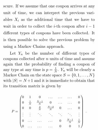
Let Yn be the number of different types ofcoupons collected after n units of time and assumeagain that the probability of finding a coupon ofany type at any time is p = 1

N . Yn will be clearly aMarkov Chain on the state space S = {0, 1, . . . , N}with |S| = N+1 and it is immediate to obtain thatits transition matrix is given by

P =

0 1 0 . . . . . . . . . 0

0 1N

N−1N

0 . . . . . . 0

0 0 2N

N−2N

0 . . . 0

......

. . .. . .

. . .. . .

...

0 . . . . . . . . . 0 N−1N

1N

0 . . . . . . . . . 0 0 1

.

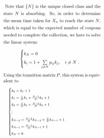
Note that {N} is the unique closed class and the

state N is absorbing. So, in order to determine

the mean time taken for Xn to reach the state N ,

which is equal to the expected number of coupons

needed to complete the collection, we have to solve

the linear system:kN = 0

ki = 1 +∑j 6=N

pijkj , i 6= N .

Using the transition matrix P , this system is equiv-alent to

k0 = k1 + 1

k1 = 1Nk1 +

N−1N

k2 + 1

k2 = 2Nk2 +

N−2N

k3 + 1

...

kN−2 = N−2N

kN−2 +2NkN−1 + 1

kN−1 = N−1N

kN−1 + 1

kN = 0

⇐⇒

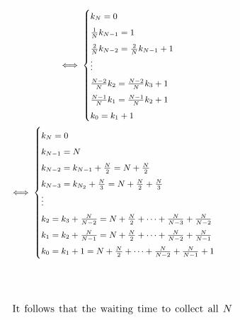
kN = 0

1NkN−1 = 1

2NkN−2 = 2

NkN−1 + 1

...N−2N

k2 = N−2N

k3 + 1

N−1N

k1 = N−1N

k2 + 1

k0 = k1 + 1

⇐⇒

kN = 0

kN−1 = N

kN−2 = kN−1 +N2= N + N

2

kN−3 = kN2 + N3= N + N

2+ N

3

...

k2 = k3 +NN−2

= N + N2+ · · ·+ N

N−3+ N

N−2

k1 = k2 +NN−1

= N + N2+ · · ·+ N

N−2+ N

N−1

k0 = k1 + 1 = N + N2+ · · ·+ N

N−2+ N

N−1+ 1

It follows that the waiting time to collect all N

coupons is given by

k0 = N

N∑i=1

1

i.

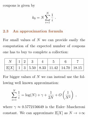
2.3 An approximation formula

For small values of N we can provide easily the

computation of the expected number of coupons

one has to buy to complete a collection:

N 1 2 3 4 5 6 7

E[X] 1 3 5.50 8.33 11.42 14.70 18.15

For bigger values of N we can instead use the fol-

lowing well known approximation:

N∑i=1

1

i= log(N) + γ +

1

2N+O

(1

N2

),

where γ ≈ 0.5772156649 is the Euler–Mascheroni

constant. We can approximate E[X] as N → +∞

by:

E[X] = N log(N)+Nγ+1

2+O

(1

N

), N → +∞ .

E.g. if N = 100, thanks to Matlab it’s possi-

ble to evaluate the waiting time to complete the

collection and to compare this with the asymp-

totic expansion. If N = 100, the exact evaluation

gives E[X] = 518.7377 ± 10−4, while the evalu-

ation of N log(N) + Nγ + 12 at N = 100 gives

518.7385 ± 10−4 as an approximation of the value

of E[X]. The exact and approximated values of

E[X] up to N = 100 are plotted in Figure 1.

Note that the exact computation in this case

can be carried out up to big values of N , but this

will not be true in the case of unequal probabilities,

that we will consider in the next section.

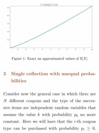
Figure 1: Exact an approximated values of E[X]

3 Single collection with unequal proba-bilities

Consider now the general case in which there are

N different coupons and the type of the succes-

sive items are independent random variables that

assume the value k with probability pk no more

constant. Here we will have that the i-th coupon

type can be purchased with probability pi ≥ 0,

with p1 + · · ·+pN = 1. This is clearly the most re-

alistic case, since in any collection there are “rare”

coupons that makes the average number of coupons

needed bigger and bigger. Our goal here is to find

the expected number of coupons that we have to

buy to complete the collection and we will recall a

known formula (see e.g. Ross [8]), present a new

formula (obtained in [2]) and a possible approxi-

mation procedure, outlined in the case of the Man-

delbrot distribution.

3.1 The Maximum-Minimums Identity ap-

proach

Let us now denote by Xi the random number ofcoupons we need to buy to obtain the first couponof type i. The waiting time to complete the col-lection is therefore given by the random variableX = max{X1, . . . , XN}. Note that Xi is a geo-metric random variable with parameter pi (because

each new coupon obtained is of type i with prob-ability pi), but now these variables are no moreindependent. Since the minimum of Xi and Xj isthe number of coupons needed to obtain either acoupon of type i or a coupon of type j, it followsthat for i 6= j, min(Xi, Xj) is a geometric ran-dom variable with parameter pi + pj and the sameholds true for the minimum of any finite number ofthese random variables. To compute the expectedvalue of the random variable X, we will use theMaximum-Minimums Identity, whose proof can befound e.g. in [8]:

E[X] = E[

maxi=1,...,N

Xi

]=∑i

E[Xi]−∑i<j

E[min(Xi, Xj)]

+∑i<j<k

E[min(Xi, Xj , Xk)]− . . .

· · ·+ (−1)N+1E[min(X1, X2, . . . , XN )]

=∑i

1

pi−∑i<j

1

pi + pj+∑i<j<k

1

pi + pj + pk− . . .

· · ·+ (−1)N+1 1

p1 + · · ·+ pN.

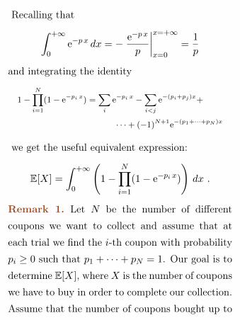
Recalling that∫ +∞

0e−p x dx = − e−p x

p

∣∣∣∣x=+∞

x=0

=1

p

and integrating the identity

1−N∏i=1

(1− e−pi x) =∑i

e−pi x −∑i<j

e−(pi+pj)x+

· · ·+ (−1)N+1e−(p1+···+pN )x

we get the useful equivalent expression:

E[X] =

∫ +∞

0

(1−

N∏i=1

(1− e−pi x)

)dx .

Remark 1. Let N be the number of different

coupons we want to collect and assume that at

each trial we find the i-th coupon with probability

pi ≥ 0 such that p1 + · · ·+ pN = 1. Our goal is to

determine E[X], where X is the number of coupons

we have to buy in order to complete our collection.

Assume that the number of coupons bought up to

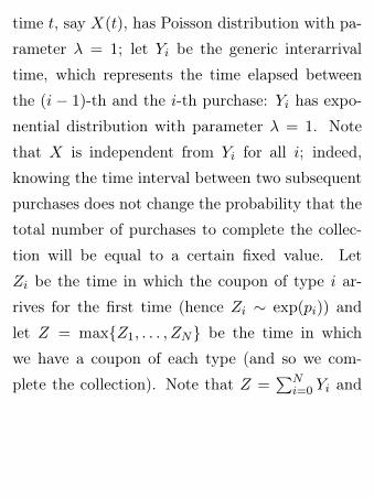
time t, say X(t), has Poisson distribution with pa-

rameter λ = 1; let Yi be the generic interarrival

time, which represents the time elapsed between

the (i − 1)-th and the i-th purchase: Yi has expo-

nential distribution with parameter λ = 1. Note

that X is independent from Yi for all i; indeed,

knowing the time interval between two subsequent

purchases does not change the probability that the

total number of purchases to complete the collec-

tion will be equal to a certain fixed value. Let

Zi be the time in which the coupon of type i ar-

rives for the first time (hence Zi ∼ exp(pi)) and

let Z = max{Z1, . . . , ZN} be the time in which

we have a coupon of each type (and so we com-

plete the collection). Note that Z =∑N

i=0 Yi and

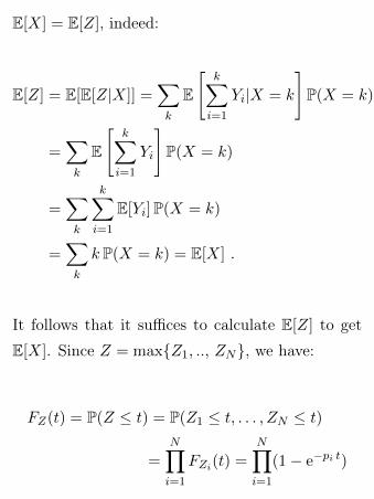
E[X] = E[Z], indeed:

E[Z] = E[E[Z|X]] =∑k

E

[k∑i=1

Yi|X = k

]P(X = k)

=∑k

E

[k∑i=1

Yi

]P(X = k)

=∑k

k∑i=1

E[Yi]P(X = k)

=∑k

k P(X = k) = E[X] .

It follows that it suffices to calculate E[Z] to get

E[X]. Since Z = max{Z1, .., ZN}, we have:

FZ(t) = P(Z ≤ t) = P(Z1 ≤ t, . . . , ZN ≤ t)

=

N∏i=1

FZi(t) =

N∏i=1

(1− e−pi t)

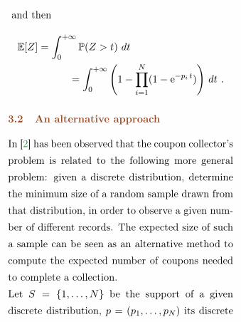
and then

E[Z] =

∫ +∞

0P(Z > t) dt

=

∫ +∞

0

(1−

N∏i=1

(1− e−pi t)

)dt .

3.2 An alternative approach

In [2] has been observed that the coupon collector’s

problem is related to the following more general

problem: given a discrete distribution, determine

the minimum size of a random sample drawn from

that distribution, in order to observe a given num-

ber of different records. The expected size of such

a sample can be seen as an alternative method to

compute the expected number of coupons needed

to complete a collection.

Let S = {1, . . . , N} be the support of a given

discrete distribution, p = (p1, . . . , pN ) its discrete

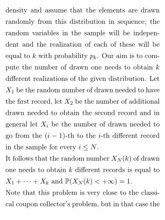
density and assume that the elements are drawn

randomly from this distribution in sequence; the

random variables in the sample will be indepen-

dent and the realization of each of these will be

equal to k with probability pk. Our aim is to com-

pute the number of drawn one needs to obtain k

different realizations of the given distribution. Let

X1 be the random number of drawn needed to have

the first record, let X2 be the number of additional

drawn needed to obtain the second record and in

general let Xi be the number of drawn needed to

go from the (i − 1)-th to the i-th different record

in the sample for every i ≤ N .

It follows that the random numberXN (k) of drawn

one needs to obtain k different records is equal to

X1 + · · ·+Xk and P(XN (k) < +∞) = 1.

Note that this problem is very close to the classi-

cal coupon collector’s problem, but in that case the

random variablesXi denote the number of coupons

one has to buy to go from the (i − 1)-th to the i-

th different type of coupon in the collection and

XN (N) represents the number of coupons one has

to buy to complete the collection.

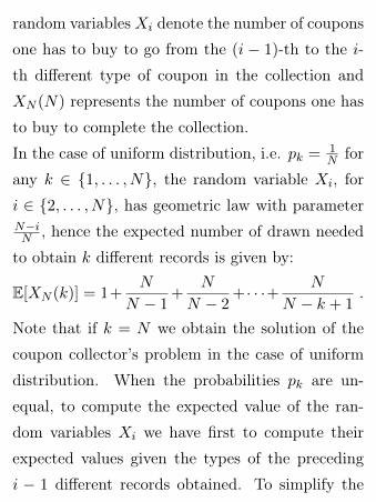
In the case of uniform distribution, i.e. pk = 1N for

any k ∈ {1, . . . , N}, the random variable Xi, for

i ∈ {2, . . . , N}, has geometric law with parameterN−iN , hence the expected number of drawn needed

to obtain k different records is given by:

E[XN (k)] = 1+N

N − 1+

N

N − 2+ · · ·+ N

N − k + 1.

Note that if k = N we obtain the solution of the

coupon collector’s problem in the case of uniform

distribution. When the probabilities pk are un-

equal, to compute the expected value of the ran-

dom variables Xi we have first to compute their

expected values given the types of the preceding

i − 1 different records obtained. To simplify the

notation, define p(i1, . . . , ik) = 1 − pi1 − · · · − pikfor k ≤ N and different indexes i1, i2, . . . , ik. It

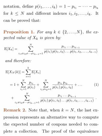
can be proved that:

Proposition 1. For any k ∈ {2, . . . , N}, the ex-pected value of Xk is given by:

E[Xk] =N∑

i1 6=i2 6=···6=ik−1=1

pi1 . . . pik−1

p(i1) p(i1, i2) . . . p(i1, i2, . . . , ik−1)

and therefore:

E[XN (k)] =

k∑s=1

E[Xs]

= 1 +N∑i1=1

pi1p(i1)

+N∑

i1 6=i2=1

pi1 pi2p(i1) p(i1, i2)

+ . . . (1)

+

N∑i1 6=i2 6=···6=ik−1=1

pi1 . . . pik−1

p(i1) p(i1, i2) . . . p(i1, i2, . . . , ik−1).

Remark 2. Note that, when k = N , the last ex-

pression represents an alternative way to compute

the expected number of coupons needed to com-

plete a collection. The proof of the equivalence

between the last expression with k = N and the

formula obtained using the Maximum-Minimums

Identity is not trivial; furthermore, both expres-

sions are not computable for large values of k.

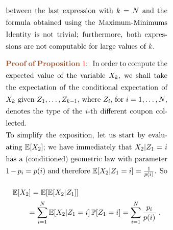
Proof of Proposition 1: In order to compute the

expected value of the variable Xk, we shall take

the expectation of the conditional expectation of

Xk given Z1, . . . , Zk−1, where Zi, for i = 1, . . . , N ,

denotes the type of the i-th different coupon col-

lected.

To simplify the exposition, let us start by evalu-

ating E[X2]; we have immediately that X2|Z1 = i

has a (conditioned) geometric law with parameter

1− pi = p(i) and therefore E[X2|Z1 = i] = 1p(i) . So

E[X2] = E[E[X2|Z1]]

=N∑i=1

E[X2|Z1 = i]P[Z1 = i] =N∑i=1

pip(i)

.

Let us now take k ∈ {3, . . . , N}: it is easy to seethat

E[Xk] = E[E[Xk|Z1, Z2, . . . , Zk−1]]

=

N∑i1 6=i2 6=···6=ik−1=1

E[Xk|Z1 = i1, , Z2 = i2, · · · , Zk−1 = ik−1]

× P[Z1 = i1, ..., Zk−1 = ik−1] .

Note that P[Zi = Zj ] = 0 for any i 6= j. The con-ditional law of Xk|Z1 = i1, Z2 = i2, · · · , Zk−1 =

ik−1, for i1 6= i2 6= · · · 6= ik−1, is that of a geomet-ric random variable with parameter p(i1, . . . , ik−1)and its conditional expectation is p(i1, . . . , ik−1)−1.By the multiplication rule, we get

P[Z1 =i1, . . . , Zk−1 = ik−1]

= P[Z1 = i1]× P[Z2 = i2|Z1 = i1]×

· · · × P[Zk−1 = ik−1|Z1 = i1, . . . , Zk−2 = ik−2] .

Note that, even though the types of the succes-sive coupons are independent random variables,the random variables Zi are not mutually inde-pendent. A simple computation gives, for any

s = 2, . . . , k − 1, that

P[Zs = is|Z1 = i1, . . . , Zs−1 = is−1] =pis

1− pi1 − . . .− pis−1

if i1 6= i2 6= · · · 6= ik−1 and zero otherwise. Recall-ing the compact notation p(i1, . . . , ik) = 1− pi1 −. . .− pik , we then get

E[Xk] =

N∑i1 6=i2 6=···6=ik−1=1

pi1 pi2 · · · pik−1

p(i1) p(i1, i2) · · · p(i1, i2, . . . , ik−1)

and the proof is complete.

3.3 An approximation procedure via the

Heaps’ law in natural languages

In [2] Ferrante and Frigo proposed the following

procedure in order to approximate the expected

number of coupons needed to complete a collection

in the unequal case.

Let us consider a text written in a natural lan-

guage: the Heaps’ law is an empirical law which

describes the portion of the vocabulary which is

used in the given text. This law can be described

by the following formula

E[Rm(n)] ∼ K nβ

where Rm(n) is the (random) number of different

words presents in a text consisting of n words and

taken from a vocabulary of m words, while K and

β are free parameters determined empirically. In

order to obtain a formal derivation of this empirical

law, van Leijenhorst and van der Weide in [5] have

considered the average growth in the number of

records, when elements are drawn randomly from

some statistical distribution that can assume ex-

actly m different values. The exact computation of

the average number of records in a sample of size n,

E[Rm(n)], can be easily obtained using the follow-

ing approach. Let S = {1, 2, . . . ,m} be the supportof the given distribution, define X = m − Rm(n)

the number of values in S not observed and denote

by Ai the event that the record i is not observed.

It is immediate to see that P[Ai] = (1 − pi)n,

X =∑m

i=1 1Ai and therefore that

E[Rm(n)] = m− E[X] = m−m∑i=1

(1− pi)n . (2)

Assuming now that the elements are drawn ran-

domly from the Mandelbrot distribution, van Lei-

jenhorst and van der Weide obtain that the Heaps’

law is asymptotically true as n andm go to infinity

and n � mθ−1, where θ is one of the parameters

of the Mandelbrot distribution (see [5] for the de-

tails).

It is possible to relate this problem with the

previous one: assume that we are interested in the

minimum number Xm(k) of elements that we have

to draw randomly from a given statistical distri-

bution in order to obtain k different records. This

is clearly strictly related to the previous problem

and at first sight one expects that the technical dif-

ficulties would be similar. However, we have just

proved that the computation of the expectation of

Xm(k) is much more complicated. The formula

that we obtained before is computationally hard

and we are able to perform the exact computa-

tion in the environment R just for distributions

with a support of small cardinality. An approxi-

mation procedure can be obtained in the special

case of the Mandelbrot distribution, widely used

in the applications, making use of the asymptotic

results proved in [5] in order to derive the Heaps’

law.

The exact formula we obtained in the previous

section is nice, but it is tremendously heavy to com-

pute as soon as the cardinality of the support of the

distribution becomes larger then 10. The number

of all possible ordered choices of indexes sets in-

volved in (1) increases very fast with k leading the

objects hard to handle with a personal computer.

For this reason it would be important to be able to

approximate this formula, at least in some cases of

interest, even if its complicated structure may sug-

gest that it could be quite difficult in general. In

this section we shall consider the case of the Man-

delbrot distribution, which is commonly used in the

Heaps’ law and other practical problems. Applying

the results proved in [5], we present here a possible

strategy to approximate the expectation of Xm(k)

and present some numerical approximation in or-

der to test our procedure. Let us consider Rm(n)

andXm(k): these two random variables are strictly

related, since [Rm(n) > k] = [Xm(k) < n], for

k ≤ n ≤ m. However, we have seen that the com-

putation of their expected values is quite different.

With an abuse of language, we could say that the

two functions n 7→ E[Rm(n)] and k 7→ E[Xm(k)]

represent one the “inverse” of the other. In order

to confirm this statement, let us consider the case

studied in [5], i.e. let us assume to sample from

the Mandelbrot distribution. Fixed three parame-

ters m ∈ N, θ ∈ [1, 2] and c ≥ 0, we shall assume

that S = {1, . . . ,m} and

pi = am(c+i)−θ , am =

(m∑i=1

(c+ i)−θ

)−1. (3)

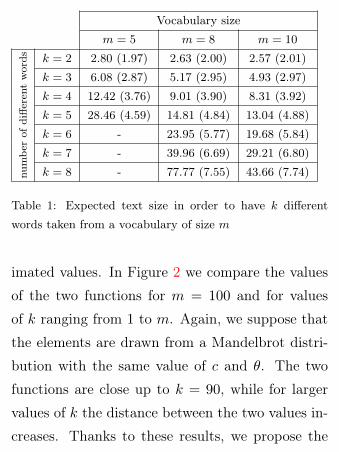
We implement both the expressions (2) and (1) us-

ing the environment R. We set the parameters of

the Mandelbrot distribution to be c = 0.30 and

θ = 1.75. Using (1), we compute the expected

number E[Xm(k)] of elements we have to draw ran-

domly from a Mandelbrot distribution in order to

obtain k different records, for three levels of m, be-

ing m the vocabulary size, i.e the maximum size of

different words. In brackets we show the expected

number of different words in a random selection of

exactly E[Xm(k)] elements, computed using (2).

Results are collected in Table 1. We see that the

number of different words we expect in a text size

of dimension E[Xm(k)] is close to the value of k

and this supports our statement about the connec-

tion between E[Rm(n)] and E[Xm(k)]. As under-

lined before, we can compute these expectations

only for small values of k.

At the same time, since E[Rm(n)] ≤ m, it is

clear that our statement that n 7→ E[Rm(n)] and

k 7→ E[Xm(k)] represent one the “inverse” of the

other could be valid just for values of k small with

respect to m. This idea arises also from Table 1,

but in order to confirm this we shall compare the

two functions for larger values of m. Since our for-

mula is not computable for values larger than 10,

we shall perform a simulation to obtain its approx-

Vocabulary size

m = 5 m = 8 m = 10

numbe

rof

diffe

rent

words k = 2 2.80 (1.97) 2.63 (2.00) 2.57 (2.01)

k = 3 6.08 (2.87) 5.17 (2.95) 4.93 (2.97)

k = 4 12.42 (3.76) 9.01 (3.90) 8.31 (3.92)

k = 5 28.46 (4.59) 14.81 (4.84) 13.04 (4.88)

k = 6 - 23.95 (5.77) 19.68 (5.84)

k = 7 - 39.96 (6.69) 29.21 (6.80)

k = 8 - 77.77 (7.55) 43.66 (7.74)

Table 1: Expected text size in order to have k different

words taken from a vocabulary of size m

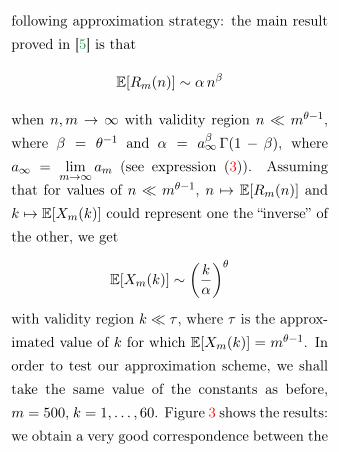
imated values. In Figure 2 we compare the values

of the two functions for m = 100 and for values

of k ranging from 1 to m. Again, we suppose that

the elements are drawn from a Mandelbrot distri-

bution with the same value of c and θ. The two

functions are close up to k = 90, while for larger

values of k the distance between the two values in-

creases. Thanks to these results, we propose the

following approximation strategy: the main result

proved in [5] is that

E[Rm(n)] ∼ αnβ

when n,m → ∞ with validity region n � mθ−1,

where β = θ−1 and α = aβ∞ Γ(1 − β), where

a∞ = limm→∞

am (see expression (3)). Assuming

that for values of n � mθ−1, n 7→ E[Rm(n)] and

k 7→ E[Xm(k)] could represent one the “inverse” of

the other, we get

E[Xm(k)] ∼(k

α

)θwith validity region k � τ , where τ is the approx-

imated value of k for which E[Xm(k)] = mθ−1. In

order to test our approximation scheme, we shall

take the same value of the constants as before,

m = 500, k = 1, . . . , 60. Figure 3 shows the results:

we obtain a very good correspondence between the

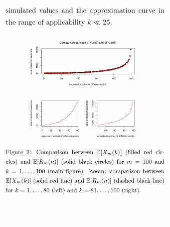
simulated values and the approximation curve in

the range of applicability k � 25.

0 20 40 60 80 100

050

0015

000

Comparison between E(Xm(k)) and E(Rm(n))

expected number of different words

size

of r

ando

m s

elec

tion

0 20 40 60 80

010

0020

00

expected number of different words

size

of r

ando

m s

elec

tion

85 90 95 100

4000

8000

1400

0

expected number of different words

size

of r

ando

m s

elec

tion

Figure 2: Comparison between E[Xm(k)] (filled red cir-

cles) and E[Rm(n)] (solid black circles) for m = 100 and

k = 1, . . . , 100 (main figure). Zoom: comparison between

E[Xm(k)] (solid red line) and E[Rm(n)] (dashed black line)

for k = 1, . . . , 80 (left) and k = 81, . . . , 100 (right).

0 10 20 30 40 50 60

010

020

030

040

050

060

0

Comparison between E(Xm(k)) and Heaps’ Law

expected number of different words

size

of r

ando

m s

elec

tion

Figure 3: Comparison between E[Xm(k)] (filled black cir-

cles) and (k/α)θ (solid red line) for m = 500 and k =

1, . . . , 60.

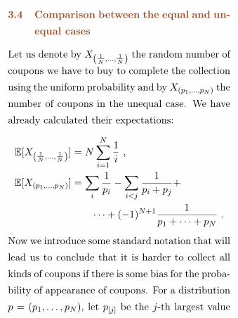
3.4 Comparison between the equal and un-

equal cases

Let us denote by X( 1N,..., 1

N ) the random number of

coupons we have to buy to complete the collection

using the uniform probability and byX(p1,...,pN ) the

number of coupons in the unequal case. We have

already calculated their expectations:

E[X( 1N,..., 1

N )] = N

N∑i=1

1

i,

E[X(p1,...,pN )] =∑i

1

pi−∑i<j

1

pi + pj+

· · ·+ (−1)N+1 1

p1 + · · ·+ pN.

Now we introduce some standard notation that will

lead us to conclude that it is harder to collect all

kinds of coupons if there is some bias for the proba-

bility of appearance of coupons. For a distribution

p = (p1, . . . , pN ), let p[j] be the j-th largest value

of {p1, . . . , pN}, that is p[1] ≥ p[2] ≥ · · · ≥ p[N ].

We say that a distribution p = (p1, . . . , pN ) is ma-

jorized by a distribution q = (q1, . . . , qN ), and we

write p ≺ q, ifk∑i=1

p[i] ≤k∑j=1

q[j] for all 1 ≤ k ≤

N − 1. Let us prove that(1N , . . . ,

1N

)≺ p for any

distribution p = (p1, . . . , pN ). Indeed, since p is a

distribution, we have that p[1] ≥ 1N . Let now as-

sume that there exists 1 < k ≤ N − 1 such thatk∑i=1

p[i] <kN . This implies that

N∑i=k+1

p[i] >N−kN ,

which in turn implies that there exists j ∈ {k +

1, . . . , N} such that p[j] > 1N , which leads to a con-

tradiction with the fact thatk∑i=1

p[i] <kN .

We say that the symmetric function f(p) de-

fined on a distribution is Schur convex (resp. con-

cave) if p ≺ q =⇒ f(p) ≤ f(q) (resp. f(p) ≥f(q)). Finally, we say that a random variable X is

stochastically smaller than a random variable Y if

P(X > a) ≤ P(Y > a) for all real a. The following

results have been proved in [6]:

Theorem 1. The probability P(Xp ≤ n) is a Schur

concave function of p.

Corollary 1. If p ≺ q, then Xp is stochasti-

cally smaller than Xq. In particular: X( 1N,..., 1

N )is stochastically smaller than Xp for all p.

Corollary 2. The expectation E[Xp] is a Schur

convex function of p. In particular: E[X( 1N,..., 1

N )] ≤E[X(p1,...,pN )] for all p.

3.5 Examples

• N = 2, E[X( 12, 12)] = 3

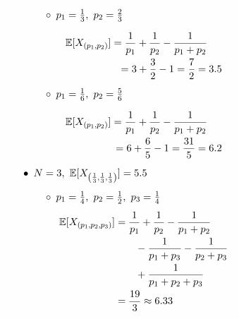
◦ p1 = 13 , p2 = 2

3

E[X(p1,p2)] =1

p1+

1

p2− 1

p1 + p2

= 3 +3

2− 1 =

7

2= 3.5

◦ p1 = 16 , p2 = 5

6

E[X(p1,p2)] =1

p1+

1

p2− 1

p1 + p2

= 6 +6

5− 1 =

31

5= 6.2

• N = 3, E[X( 13, 13, 13)] = 5.5

◦ p1 = 14 , p2 = 1

2 , p3 = 14

E[X(p1,p2,p3)] =1

p1+

1

p2− 1

p1 + p2

− 1

p1 + p3− 1

p2 + p3

+1

p1 + p2 + p3

=19

3≈ 6.33

◦ p1 = 16 , p2 = 4

6 , p3 = 16

E[X(p1,p2,p3)] =1

p1+

1

p2− 1

p1 + p2

− 1

p1 + p3− 1

p2 + p3

+1

p1 + p2 + p3

=91

10= 9.1 .

In Figure 4 we show the value of E[X] for dif-

ferent choices of p1 (p2 = 1−p1) in the case N = 2,

while in Figure 5 we show some level curves of E[X]

for different choices of p1 and p2 (p3 = 1− p1− p2)in the case N = 3.

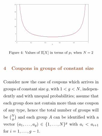
Figure 4: Values of E[X] in terms of p1 when N = 2

4 Coupons in groups of constant size

Consider now the case of coupons which arrives in

groups of constant size g, with 1 < g < N , indepen-

dently and with unequal probabilities; assume that

each group does not contain more than one coupon

of any type, hence the total number of groups will

be(Ng

)and each group A can be identified with a

vector (a1, . . . , ag) ∈ {1, . . . , N}g with ai < ai+1

for i = 1, . . . , g − 1.

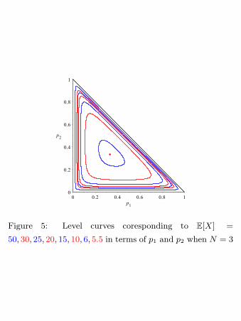
Figure 5: Level curves coresponding to E[X] =

50, 30, 25, 20, 15, 10, 6, 5.5 in terms of p1 and p2 when N = 3

Moreover, assume that the type of successive groups

of coupons that one collects form a sequence of in-

dependent random variables.

To study the unequal probabilities case, we first

order the groups according to the lexicographical

order (i.e. A = (a1, . . . , ag) < B = (b1, . . . , bg) if

there exists i ∈ {1, . . . , g− 1} such that as = bs for

s < i and ai < bi).

We denote by qi, i ∈{

1, . . . ,(Ng

)}, the probabil-

ity to purchase (at any given time) the i-th group

of coupons, according to the lexicographical or-

der, and given k ∈ {1, . . . , N − g} we denote by

q(i1, . . . , ik) the probability to purchase a group of

coupons which does not contain any of the coupons

i1, . . . , ik.

To compute the probabilities q(i1, . . . , ik)’s,

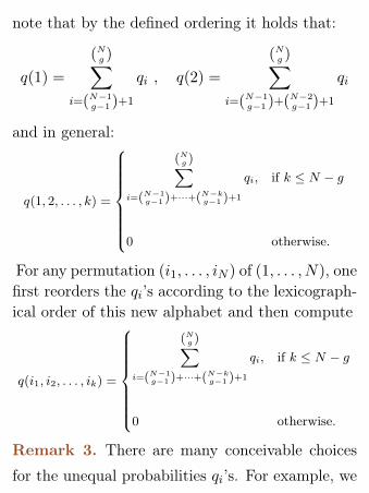
note that by the defined ordering it holds that:

q(1) =

(Ng )∑i=(N−1

g−1 )+1

qi , q(2) =

(Ng )∑i=(N−1

g−1 )+(N−2g−1 )+1

qi

and in general:

q(1, 2, . . . , k) =

(Ng )∑i=(N−1

g−1 )+···+(N−kg−1 )+1

qi, if k ≤ N − g

0 otherwise.

For any permutation (i1, . . . , iN ) of (1, . . . , N), onefirst reorders the qi’s according to the lexicograph-ical order of this new alphabet and then compute

q(i1, i2, . . . , ik) =

(Ng )∑i=(N−1

g−1 )+···+(N−kg−1 )+1

qi, if k ≤ N − g

0 otherwise.

Remark 3. There are many conceivable choices

for the unequal probabilities qi’s. For example, we

can assume that one forms the groups following the

strategy of the draft lottery in the American pro-

fessional sports, where different proportion of the

different coupons are put together and we choose

at random in sequence the coupons, discarding the

eventually duplicates, up to obtaining a group of k

coupons. Or, more simply, we can assume that the

i-th coupon will arrive with probability pi and that

the probability of any group is proportional to the

product of the probabilities of the single coupons

contained.

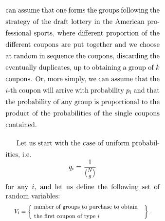
Let us start with the case of uniform probabil-

ities, i.e.

qi =1(Ng

)for any i, and let us define the following set ofrandom variables:

Vi =

{ number of groups to purchase to obtain

the first coupon of type i

}.

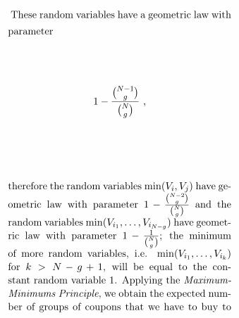
These random variables have a geometric law with

parameter

1−(N−1g

)(Ng

) ,

therefore the random variables min(Vi, Vj) have ge-

ometric law with parameter 1 − (N−2g )

(Ng )and the

random variables min(Vi1 , . . . , ViN−g) have geomet-ric law with parameter 1 − 1

(Ng ); the minimum

of more random variables, i.e. min(Vi1 , . . . , Vik)

for k > N − g + 1, will be equal to the con-stant random variable 1. Applying the Maximum-Minimums Principle, we obtain the expected num-ber of groups of coupons that we have to buy to

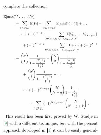
complete the collection:

E[max(V1, . . . , VN )]

=∑

1≤i≤N

E[Vi]−∑

1≤i≤j≤N

E[min(Vi, Vj)] + . . .

· · ·+ (−1)N−g+1∑

0≤i1<i2<···<iN−g≤N

E[Vi1 , . . . , ViN−g+1 ]

+ (−1)N−g+2∑

0≤i1<i2<···<iN−g+1≤N

1 + · · ·+ (−1)N+1

=

(N

1

)1

1− (N−1g )

(Ng )

−

(N

2

)1

1− (N−2g )

(Ng )

+

(N

3

)1

1− (N−3g )

(Ng )

− . . .

· · ·+ (−1)N−g+1

(N

N − g

)1

1− 1

(Ng )

+∑

1≤k≤g

(−1)N−g+k+1

(N

N − g + k

).

This result has been first proved by W. Stadje in

[9] with a different technique, but with the present

approach developed in [1] it can be easily general-

ized to the unequal probabilities case as follows:

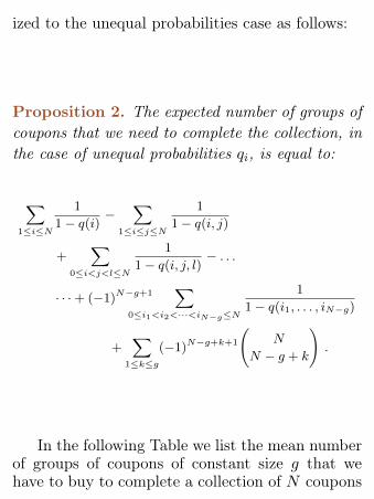
Proposition 2. The expected number of groups ofcoupons that we need to complete the collection, inthe case of unequal probabilities qi, is equal to:

∑1≤i≤N

1

1− q(i) −∑

1≤i≤j≤N

1

1− q(i, j)

+∑

0≤i<j<l≤N

1

1− q(i, j, l) − . . .

· · ·+ (−1)N−g+1∑

0≤i1<i2<···<iN−g≤N

1

1− q(i1, . . . , iN−g)

+∑

1≤k≤g

(−1)N−g+k+1

(N

N − g + k

).

In the following Table we list the mean numberof groups of coupons of constant size g that wehave to buy to complete a collection of N coupons

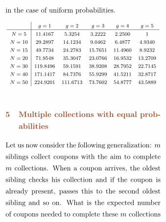
in the case of uniform probabilities.

g = 1 g = 2 g = 3 g = 4 g = 5

N = 5 11.4167 5.3254 3.2222 2.2500 1

N = 10 29.2897 14.1234 9.0462 6.4877 4.9340

N = 15 49.7734 24.2783 15.7651 11.4960 8.9232

N = 20 71.9548 35.3047 23.0766 16.9532 13.2709

N = 30 119.8496 59.1591 38.9208 28.7952 22.7145

N = 40 171.1417 84.7376 55.9299 41.5211 32.8717

N = 50 224.9201 111.6713 73.7602 54.8777 43.5889

5 Multiple collections with equal prob-abilities

Let us now consider the following generalization: m

siblings collect coupons with the aim to complete

m collections. When a coupon arrives, the oldest

sibling checks his collection and if the coupon is

already present, passes this to the second oldest

sibling and so on. What is the expected number

of coupons needed to complete these m collections

in this collaborative setting? For sure this number

will be smaller than m times the average number

of coupons needed to complete a single collection,

but how difficult even if possible will be the exact

computation? In the equal case we will present the

exact solution, known in the literature since 1960,

and for the unequal case we will present an upper

bound and the exact solution via the Markovian

approach. Both these results are to the best of our

knowledge original, or at least difficult to be found

in the existing literature.

5.1 General solution

The solution to the problem of determining the

mean time to complete m sets of N equally likely

coupons was found in 1960 by D. J. Newman and

L. Shepp.

Assume we want to collect m sets of N equally

likely coupons and let pi be the probability of fail-

ure of obtaining m sets up to and including the

purchase of the i-th coupon. Then, denoting by

X the random number of coupons needed to com-

pletem sets, its expectation E[X] is equal to+∞∑i=0

pi.

Note that pi = Mi

N i , whereMi is the number of ways

that the purchase of the i-th coupon can fail to

yield m copies of each of the N coupons in the set.

If we represent the coupons by x1, . . . , xN , then

Mi = (x1 + · · ·+ xN )i expanded and evaluated at

(1, . . . , 1) after all the terms have been removed

which have each exponent for each variable larger

thanm−1. Considerm fixed and introduce the fol-

lowing notation: if P (x1, . . . , xN ) is a polynomial

(or a power series) we define {P (x1, . . . , xN )} to be

the polynomial (or series) resulting when all terms

having all exponents greater or equal to m have

been removed. In terms of this notation, pi equals

to {(x1+···+xN )i}N i evaluated at x1 = · · · = xN = 1.

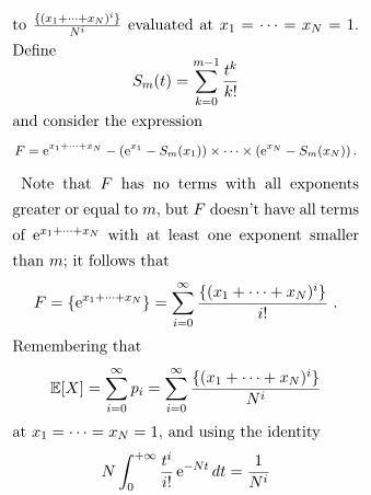
Define

Sm(t) =

m−1∑k=0

tk

k!

and consider the expression

F = ex1+···+xN − (ex1 − Sm(x1))× · · · × (exN − Sm(xN )) .

Note that F has no terms with all exponents

greater or equal to m, but F doesn’t have all terms

of ex1+···+xN with at least one exponent smaller

than m; it follows that

F = {ex1+···+xN } =

∞∑i=0

{(x1 + · · ·+ xN )i}i!

.

Remembering that

E[X] =

∞∑i=0

pi =

∞∑i=0

{(x1 + · · ·+ xN )i}N i

at x1 = · · · = xN = 1, and using the identity

N

∫ +∞

0

ti

i!e−Nt dt =

1

N i

it follows that∞∑i=0

{(x1 + · · ·+ xN )i}N i

=

∞∑i=0

({(x1 + · · ·+ xN )i}N

∫ +∞

0

ti

i!e−N t dt

)

= N

∫ +∞

0

∞∑i=0

({(x1 + · · ·+ xN )i} t

i

i!

)e−N t dt

= N

∫ +∞

0

[et (x1+···+xN ) −

(et x1 − Sm(t x1)

)× . . .

· · · ×(et xN − Sm(t xN )

)]e−N t dt .

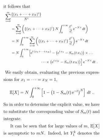
We easily obtain, evaluating the previous expres-

sions for x1 = · · · = xN = 1,

E[X] = N

∫ +∞

0

[1−

(1− Sm(t) e−t

)N]dt .

So in order to determine the explicit value, we have

to substitute the corresponding value of Sm(t) and

integrate.

It can be seen that for large values of m, E[X]

is asymptotic to mN . Indeed, let Y k1 denotes the

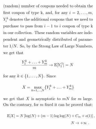
(random) number of coupons needed to obtain the

first coupon of type k, and, for any i = 2, . . . ,m,

Y ki denotes the additional coupons that we need to

purchase to pass from i − 1 to i coupon of type k

in our collection. These random variables are inde-

pendent and geometrically distributed of parame-

ter 1/N . So, by the Strong Law of Large Numbers,

we get that

Y k1 + . . .+ Y k

m

m→ E[Y 1

1 ] = N

for any k ∈ {1, . . . , N}. Since

X = maxk=1,...,N

{Y k1 + . . .+ Y k

m}

we get that X is asymptotic to mN for m large.On the contrary, for m fixed it can be proved that:

E[X] = N [log(N) + (m− 1) log log(N) + Cm + o(1)] ,

N → +∞ .

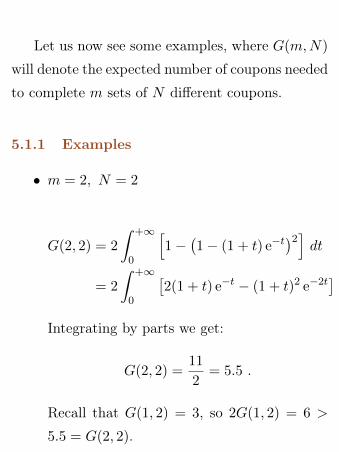
Let us now see some examples, where G(m,N)

will denote the expected number of coupons needed

to complete m sets of N different coupons.

5.1.1 Examples

• m = 2, N = 2

G(2, 2) = 2

∫ +∞

0

[1−

(1− (1 + t) e−t

)2]dt

= 2

∫ +∞

0

[2(1 + t) e−t − (1 + t)2 e−2t

]dt .

Integrating by parts we get:

G(2, 2) =11

2= 5.5 .

Recall that G(1, 2) = 3, so 2G(1, 2) = 6 >

5.5 = G(2, 2).

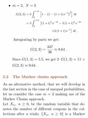
• m = 2, N = 3

G(2, 3) = 3

∫ +∞

0

[1−

(1− (1 + t) e−t

)3]dt

= 3

∫ +∞

0

[(1 + t)3 e−3t − 3 (1 + t)2 e−2t

+3 (1 + t) e−t]dt .

Integrating by parts we get:

G(2, 3) =347

36≈ 9.64 .

Since G(1, 3) = 5.5, we get 2 ·G(1, 3) = 11 >

G(2, 3) ≈ 9.64 .

5.2 The Markov chains approach

As an alternative method, that we will develop inthe last section in the case of unequal probabilities,let us consider the case m = 2 making use of theMarkov Chains approach.Let Xn, n ≥ 0, be the random variable that de-notes the number of different coupons in the col-lections after n trials; {Xn, n ≥ 0} is a Markov

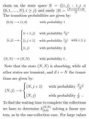
chain on the state space S = {(i, j) : i, j ∈{0, 1, . . . , N}, i ≥ j} and easily |S| = (N+1)(N+2)

2 .The transition probabilities are given by:

(0, 0) −→ (1, 0) with probability 1

(i, j) −→

(i+ 1, j) with probability N−i

N

(i, j + 1) with probability i−jN

(i, j) with probability jN

with i ≥ j

(N,N) −→ (N,N) with probability 1 .

Note that the state (N,N) is absorbing, while all

other states are transient, and if i = N the transi-

tions are given by:

(N, j) −→

(N, j + 1) with probability N−j

N

(N, j) with probability jN .

To find the waiting time to complete the collections

we have to determine k(N,N)(0,0) solving a linear sys-

tem, as in the one-collection case. For large values

of N we will need the help of a computer software,

but for small values the computation can be carried

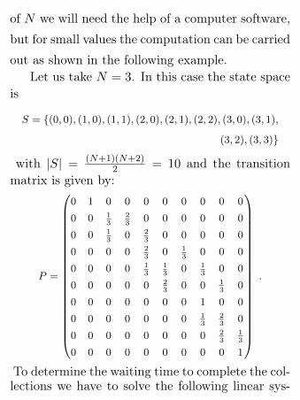
out as shown in the following example.Let us take N = 3. In this case the state space

is

S = {(0, 0), (1, 0), (1, 1), (2, 0), (2, 1), (2, 2), (3, 0), (3, 1),

(3, 2), (3, 3)}

with |S| = (N+1)(N+2)2 = 10 and the transition

matrix is given by:

P =

0 1 0 0 0 0 0 0 0 0

0 0 13

23

0 0 0 0 0 0

0 0 13

0 23

0 0 0 0 0

0 0 0 0 23

0 13

0 0 0

0 0 0 0 13

13

0 13

0 0

0 0 0 0 0 23

0 0 13

0

0 0 0 0 0 0 0 1 0 0

0 0 0 0 0 0 0 13

23

0

0 0 0 0 0 0 0 0 23

13

0 0 0 0 0 0 0 0 0 1

.

To determine the waiting time to complete the col-lections we have to solve the following linear sys-

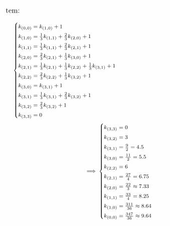
tem:

k(0,0) = k(1,0) + 1

k(1,0) = 13k(1,1) +

23k(2,0) + 1

k(1,1) = 13k(1,1) +

23k(2,1) + 1

k(2,0) = 23k(2,1) +

13k(3,0) + 1

k(2,1) = 13k(2,1) +

13k(2,2) +

13k(3,1) + 1

k(2,2) = 23k(2,2) +

13k(3,2) + 1

k(3,0) = k(3,1) + 1

k(3,1) = 13k(3,1) +

23k(3,2) + 1

k(3,2) = 23k(3,2) + 1

k(3,3) = 0

=⇒

k(3,3) = 0

k(3,2) = 3

k(3,1) =92= 4.5

k(3,0) =112

= 5.5

k(2,2) = 6

k(2,1) =274

= 6.75

k(2,0) =223≈ 7.33

k(1,1) =334

= 8.25

k(1,0) =31136≈ 8.64

k(0,0) =34736≈ 9.64

6 Multiple collections with unequal prob-abilities

To the best of our knowledge, the case of multiple

collections under the hypothesis of unequal prob-

abilities has never been considered in the litera-

ture. This is clearly a challenging problem and

it is difficult to present nice or at least exact ex-

pressions that represent the expected number of

coupons needed. In the next section, we will see

why the Maximum-Minimums approach does not

work in this case, but we will derive at least an

upper bound for the exact expected value. In the

second section we will see how, at least theoret-

ically, the Markovian approach is still applicable,

but to obtain some explicit formulas, also in the

easy cases, we need to make use of some software

likeMathematica. To conclude, we present a couple

of examples solved explicitly and derive through

simulation the value for higher values of the num-

ber of different coupons and several collections. We

provide the simulation in the cases of the uniform

distribution and the Mandelbrot distribution.

6.1 The Maximum-Minimums approach

Assume that we want to complete m sets of N

coupons in the case of unequal probabilities.

Let X1 be the random number of items that we

need to collect to obtain m copies of the first

coupon of type 1, let X2 be the number of items

that we need to collect to obtain m copies of the

first coupon of type 2 and in general let Xi be the

number of items that we need to collect to obtain

m copies of the first coupon of type i; the wait-

ing time to complete the collections is given by the

random variable X = max(X1, . . . , XN ).

To compute E[X] we can use the Maximum-

Minimums Identity, as in the single collection

case:

E[X] =∑i

E[Xi]−∑i<j

E[min(Xi, Xj)]

+∑i<j<k

E[min(Xi, Xj , Xk)] + . . .

· · ·+ (−1)N+1E[min(X1, X2, . . . , XN )] .

Note that the random variable Xi has negative bi-

nomial law with parameters (m, pi), hence E[Xi] =mpi, but now it isn’t possible to compute the ex-

act law of the random variables mini<j(Xi, Xj),

mini<j<k(Xi, Xj , Xk), . . . . However, it is possible

to prove that, for i 6= j:

E[T (i, j; 2)] ≤ E[min(Xi, Xj)] ≤ E[Z(i, j; 2)] ,

where T (i, j; 2) has negative binomial law with pa-

rameters (m, pi + pj) and Z(i, j; 2) has negative

binomial law with parameters (m+ 1, pi + pj).

In general, for 2 ≤ k ≤ N :

E[T (i1, i2, . . . , ik; k)] ≤ E[min(Xi1 , Xi2 , . . . , Xik )]

≤ E[Z(i1, i2, . . . , ik; k)] ,

where T (i1, i2, . . . , ik; k) has negative binomial law

with parameters (m, pi1+· · ·+pik) and Z(i1, i2, . . . ,

ik; k) has negative binomial law with parameters

(m(N − 1) + 1, pi1 + · · ·+ pik).

Using this consideration, we can give an upper

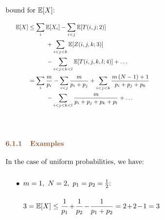
bound for E[X]:

E[X] ≤∑i

E[Xi]−∑i<j

E[T (i, j; 2)]

+∑i<j<k

E[Z(i, j, k; 3)]

−∑

i<j<k<l

E[T (i, j, k, l; 4)] + . . .

=∑i

m

pi−∑i<j

m

pi + pj+∑i<j<k

m (N − 1) + 1

pi + pj + pk

−∑

i<j<k<l

m

pi + pj + pk + pl+ . . .

6.1.1 Examples

In the case of uniform probabilities, we have:

• m = 1, N = 2, p1 = p2 = 12 :

3 = E[X] ≤ 1

p1+

1

p2− 1

p1 + p2= 2+2−1 = 3

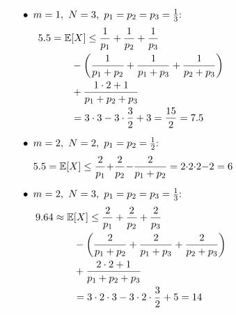
• m = 1, N = 3, p1 = p2 = p3 = 13 :

5.5 = E[X] ≤ 1

p1+

1

p2+

1

p3

−(

1

p1 + p2+

1

p1 + p3+

1

p2 + p3

)+

1 · 2 + 1

p1 + p2 + p3

= 3 · 3− 3 · 3

2+ 3 =

15

2= 7.5

• m = 2, N = 2, p1 = p2 = 12 :

5.5 = E[X] ≤ 2

p1+

2

p2− 2

p1 + p2= 2·2·2−2 = 6

• m = 2, N = 3, p1 = p2 = p3 = 13 :

9.64 ≈ E[X] ≤ 2

p1+

2

p2+

2

p3

−(

2

p1 + p2+

2

p1 + p3+

2

p2 + p3

)+

2 · 2 + 1

p1 + p2 + p3

= 3 · 2 · 3− 3 · 2 · 3

2+ 5 = 14

In the case of unequal probabilities, we have:

• m = 2, N = 2, p1 = 13 , p2 = 2

3 :

E[X] ≤ 213

+223

− 213 + 2

3

= 6 + 3− 2 = 7

• m = 2, N = 2, p1 = 16 , p2 = 5

6 :

E[X] ≤ 216

+256

− 216+ 5

6

= 12 +12

5− 2 =

62

5= 12.4

• m = 2, N = 3, p1 = 12 , p2 = 1

3 , p3 = 16 :

E[X] ≤ 212

+213

+216

−

(2

12 + 1

3

212 + 1

6

+2

13 + 1

6

)+

2 · 2 + 112 + 1

3 + 16

= 4 + 6 + 12− 12

5− 3− 4 + 5

=88

5= 17.6

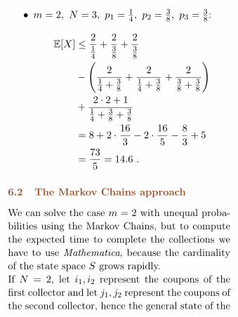
• m = 2, N = 3, p1 = 14 , p2 = 3

8 , p3 = 38 :

E[X] ≤ 214

+238

+238

−

(2

14 + 3

8

+2

14 + 3

8

+2

38 + 3

8

)+

2 · 2 + 114 + 3

8 + 38

= 8 + 2 · 16

3− 2 · 16

5− 8

3+ 5

=73

5= 14.6 .

6.2 The Markov Chains approach

We can solve the case m = 2 with unequal proba-bilities using the Markov Chains, but to computethe expected time to complete the collections wehave to use Mathematica, because the cardinalityof the state space S grows rapidly.If N = 2, let i1, i2 represent the coupons of thefirst collector and let j1, j2 represent the coupons ofthe second collector, hence the general state of the

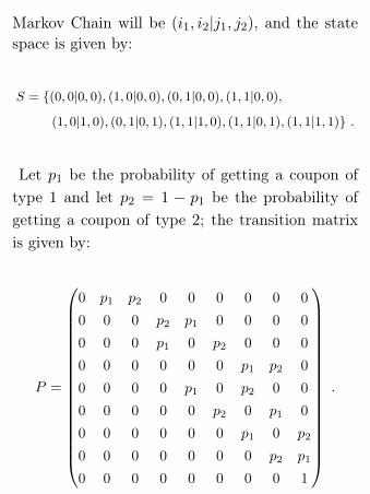
Markov Chain will be (i1, i2|j1, j2), and the statespace is given by:

S = {(0, 0|0, 0), (1, 0|0, 0), (0, 1|0, 0), (1, 1|0, 0),

(1, 0|1, 0), (0, 1|0, 1), (1, 1|1, 0), (1, 1|0, 1), (1, 1|1, 1)} .

Let p1 be the probability of getting a coupon oftype 1 and let p2 = 1 − p1 be the probability ofgetting a coupon of type 2; the transition matrixis given by:

P =

0 p1 p2 0 0 0 0 0 0

0 0 0 p2 p1 0 0 0 0

0 0 0 p1 0 p2 0 0 0

0 0 0 0 0 0 p1 p2 0

0 0 0 0 p1 0 p2 0 0

0 0 0 0 0 p2 0 p1 0

0 0 0 0 0 0 p1 0 p2

0 0 0 0 0 0 0 p2 p1

0 0 0 0 0 0 0 0 1

.

Solving the linear system

k(1,1|1,1) = 0

ki = 1 +∑

j 6=(1,1|1,1)

pijkj , i 6= (1, 1|1, 1)

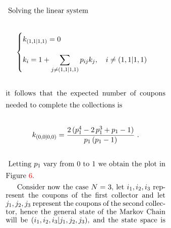
it follows that the expected number of coupons

needed to complete the collections is

k(0,0|0,0) =2 (p41 − 2 p31 + p1 − 1)

p1 (p1 − 1).

Letting p1 vary from 0 to 1 we obtain the plot in

Figure 6.Consider now the case N = 3, let i1, i2, i3 rep-

resent the coupons of the first collector and letj1, j2, j3 represent the coupons of the second collec-tor, hence the general state of the Markov Chainwill be (i1, i2, i3|j1, j2, j3), and the state space is

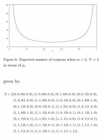
Figure 6: Expected number of coupons when m = 2, N = 2

in terms of p1

given by:

S = {(0, 0, 0|0, 0, 0), (1, 0, 0|0, 0, 0), (0, 1, 0|0, 0, 0), (0, 0, 1|0, 0, 0),

(1, 0, 0|1, 0, 0), (1, 1, 0|0, 0, 0), (1, 0, 1|0, 0, 0), (0, 1, 0|0, 1, 0),

(0, 1, 1|0, 0, 0), (0, 0, 1|0, 0, 1), (1, 1, 0|1, 0, 0), (1, 0, 1|1, 0, 0),

(1, 1, 0|0, 1, 0), (1, 1, 1|0, 0, 0), (1, 0, 1|0, 0, 1), (0, 1, 1|0, 1, 0),

(0, 1, 1|0, 0, 1), (1, 1, 0|1, 1, 0), (1, 1, 1|1, 0, 0), (1, 0, 1|1, 0, 1),

(1, 1, 1|0, 1, 0), (1, 1, 1|0, 0, 1), (0, 1, 1|0, 1, 1), (1, 1, 1|1, 1, 0),

(1, 1, 1|1, 0, 1), (1, 1, 1|0, 1, 1), (1, 1, 1|1, 1, 1)} .

Let p1 be the probability of getting a coupon of

type 1, let p2 be the probability of getting a coupon

of type 2 and let p3 = 1−p1−p2 be the probabilityof getting a coupon of type 3; the transition matrix

has order 27 and solving the linear system

k(1,1,1|1,1,1) = 0

ki = 1 +∑

j 6=(1,1,1|1,1,1)

pijkj , i 6= (1, 1, 1|1, 1, 1)

we get the expected waiting time to complete the

collections:

k(0,0,0|0,0,0) = 2

[1− 1

1− p1+

1

p1− 1

1− p2

+1

p2+

1

1− p1 − p2+

8 p31 p2 (1− p1 − p2)(1− p1)3

− 3 p41 p2 (1− p1 − p2)(1− p1)3

− 1

p1 + p2

+ p21

(−1 + 1

(1− p2)3− 6 p2 (1− p1 − p2)

(1− p1)3

+1

(p1 + p2)3

)+p1

(1− 1

(1− p2)2− 1

(p1 + p2)2

)].

Letting p1 vary from 0 to 1 and p2 from 0 to 1−p1 (to satisfy the constraint p1 +p2 ≤ 1) we obtain

the plot of the level sets of the above function in

Figure 7; the minimum of this surface corresponds

to the point (p1, p2) = (13 ,13).

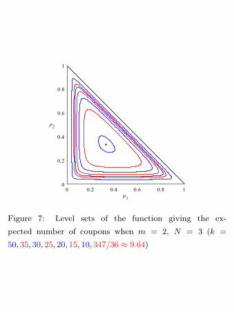
Figure 7: Level sets of the function giving the ex-

pected number of coupons when m = 2, N = 3 (k =

50, 35, 30, 25, 20, 15, 10, 347/36 ≈ 9.64)

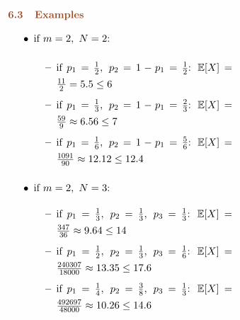
6.3 Examples

• if m = 2, N = 2:

– if p1 = 12 , p2 = 1 − p1 = 1

2 : E[X] =112 = 5.5 ≤ 6

– if p1 = 13 , p2 = 1 − p1 = 2

3 : E[X] =599 ≈ 6.56 ≤ 7

– if p1 = 16 , p2 = 1 − p1 = 5

6 : E[X] =109190 ≈ 12.12 ≤ 12.4

• if m = 2, N = 3:

– if p1 = 13 , p2 = 1

3 , p3 = 13 : E[X] =

34736 ≈ 9.64 ≤ 14

– if p1 = 12 , p2 = 1

3 , p3 = 16 : E[X] =

24030718000 ≈ 13.35 ≤ 17.6

– if p1 = 14 , p2 = 3

8 , p3 = 13 : E[X] =

49269748000 ≈ 10.26 ≤ 14.6

Note that the upper bound that we have found

using the Maximum-Minimums Identity holds.

6.4 Numerical simulation

It is clear that in the XXI Century we cannot end

this section without a numerical simulation. This

allows us to see what happens beyond the Pillars

of Hercules of our exact, even often not very useful,

explicit formulas.

0 5 10 15 20 25 30 35 40 45 500

500

1000

1500

2000

2500Uniform distribution

N

mea

n

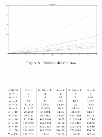
Figure 8: Uniform distribution

Uniform m = 1 2 · (m = 1) m = 2 3 · (m = 1) m = 3

N = 1 1 2 2 3 3

N = 2 3 6 5.7 9 8.04

N = 3 5.5 11 9.78 16.5 13.97

N = 4 8.3333 16.667 13.88 25 18.66

N = 5 11.4167 22.8333 20.8 34.25 26.2

N = 10 29.2897 58.5794 44.05 87.869 61.06

N = 15 49.7734 99.5469 74.76 149.3203 99.73

N = 20 71.9548 143.9096 106.75 215.8644 137.75

N = 30 119.8496 239.6992 175.82 359.5488 233.68

N = 40 171.1417 342.2834 245.39 513.4252 322.16

N = 50 224.9603 449.9205 324.96 674.8808 404.68

N = 100 518.7378 1037.5 735.06 1556.2 927.55

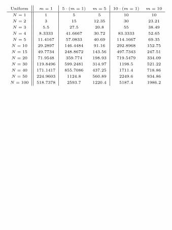
Uniform m = 1 5 · (m = 1) m = 5 10 · (m = 1) m = 10

N = 1 1 5 5 10 10

N = 2 3 15 12.35 30 23.21

N = 3 5.5 27.5 20.8 55 38.49

N = 4 8.3333 41.6667 30.72 83.3333 52.65

N = 5 11.4167 57.0833 40.69 114.1667 69.35

N = 10 29.2897 146.4484 91.16 292.8968 152.75

N = 15 49.7734 248.8672 143.56 497.7343 247.51

N = 20 71.9548 359.774 198.93 719.5479 334.09

N = 30 119.8496 599.2481 314.97 1198.5 521.22

N = 40 171.1417 855.7086 437.25 1711.4 718.86

N = 50 224.9603 1124.8 560.89 2249.6 934.86

N = 100 518.7378 2593.7 1220.4 5187.4 1986.2

0 5 10 15 20 25 30 35 40 45 500

0.5

1

1.5

2

2.5

3

3.5

4x 104 Mandelbrot distribution

N

mea

n

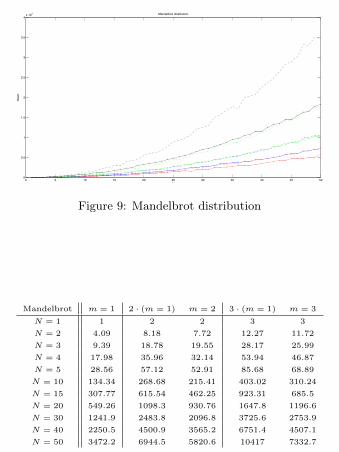
Figure 9: Mandelbrot distribution

Mandelbrot m = 1 2 · (m = 1) m = 2 3 · (m = 1) m = 3

N = 1 1 2 2 3 3

N = 2 4.09 8.18 7.72 12.27 11.72

N = 3 9.39 18.78 19.55 28.17 25.99

N = 4 17.98 35.96 32.14 53.94 46.87

N = 5 28.56 57.12 52.91 85.68 68.89

N = 10 134.34 268.68 215.41 403.02 310.24

N = 15 307.77 615.54 462.25 923.31 685.5

N = 20 549.26 1098.3 930.76 1647.8 1196.6

N = 30 1241.9 2483.8 2096.8 3725.6 2753.9

N = 40 2250.5 4500.9 3565.2 6751.4 4507.1

N = 50 3472.2 6944.5 5820.6 10417 7332.7

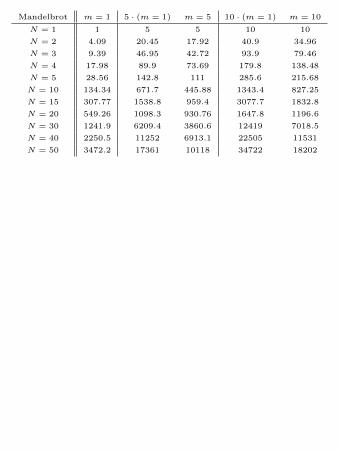
Mandelbrot m = 1 5 · (m = 1) m = 5 10 · (m = 1) m = 10

N = 1 1 5 5 10 10

N = 2 4.09 20.45 17.92 40.9 34.96

N = 3 9.39 46.95 42.72 93.9 79.46

N = 4 17.98 89.9 73.69 179.8 138.48

N = 5 28.56 142.8 111 285.6 215.68

N = 10 134.34 671.7 445.88 1343.4 827.25

N = 15 307.77 1538.8 959.4 3077.7 1832.8

N = 20 549.26 1098.3 930.76 1647.8 1196.6

N = 30 1241.9 6209.4 3860.6 12419 7018.5

N = 40 2250.5 11252 6913.1 22505 11531

N = 50 3472.2 17361 10118 34722 18202

In figures 8 and 9 we have considered the

present case with several cooperative collectors

and an arbitrary number of coupons that arrives

according to the uniform probability distribution

or to a Mandelbrot distribution with parameters

c = 0.30 and θ = 1.75. To see how big will be in

this case the expected number of coupons to be col-

lected in order to complete all the collections, we

have simulated a big number of virtual collections.

Then we have evaluated the arithmetic mean of

the number of coupons needed in these simulated

collections to complete the sets.

We also have plotted the numerical simulated

values (solid line) and compared them with m

times the expected number of coupons needed to

complete a single collection (dashed line), again

trough a simulation, to see how much money we

save in the case of a cooperative collection; in par-

ticular, we have plotted in red the case m = 2, in

blue the case m = 3, in green the case m = 5 and

in black the case m = 10.

From these computations we observe that if

N = 50, in the case of the uniform distribution

we can save about the 27% of our money in the

case of m = 2 and that this increases up to a 58%

when m = 10, while in the case of the Mandel-

brot distribution we can save about the 16% of our

money in the case of m = 2 and about the 47%

when m = 10.

References

[1] M. Ferrante, N. Frigo, A note on the coupon-

collector’s problem with multiple arrivals and the

random sampling, arXiv:1209.2667v2, 2012.

[2] M. Ferrante, N. Frigo, On the expected num-

ber of different records in a random sample,

arXiv:1209.4592v1, 2012.

[3] P. Flajolet, D. Gardy, L. Thimonier, Birthday

paradox, coupon collectors, caching algorithms

and self-organizing search, Discrete Appl. Math.,

39:207-229, 1992.

[4] L. Holst, On birthday, collectors’, occupancy

and other classical urn problems, Internat.

Statist. Rev., 54:15-27, 1986.

[5] D. van Leijenhorst, Th. van der Weide, A for-

mal derivation of Heaps’ Law, Information Sci-

ences, 170: 263-272, 2005.

[6] T. Nakata, Coupon collector’s problem with un-

like probabilities, Preprint, 2008.

[7] D. J. Newman, L. Shepp, The double dixie

cup problem, American Mathematical Monthly,

67:58-61, 1960.

[8] S. Ross, A first course in probability, 9th Edi-

tion, Pearson, 2012.

[9] W. Stadje, The collector’s problem with group

drawings, Advances in Applied Probability,

22:866-882, 1990.

[10] H. von Schelling, Coupon collecting for

unequal probabilities, American Mathematical

Monthly, 61:306-311, 1954.

Marco Ferrante

Dipartimento di Matematica

Università degli Studi di Padova

Padova, Italy

ferrante@math.unipd.it

Monica Saltalamacchia

Dipartimento di Matematica

Università degli Studi di Padova

Padova, Italy

monicasaltalamacchia@tiscali.it

Publicat el 25 de magi de 2014