Embed Size (px)
Citation preview
The Countercyclical Capital Buffer
15 February 2017
By CHRISTOPH BASTEN (FINMA) AND CATHÉRINE KOCH (BIS)*
We examine the first activation of the Countercyclical Capital Buffer (CCyB) as macroprudential
tool of Basel III. Our short-term analysis examines how banks adjust their rejections and pricing
of mortgages. We then study how bank capitalization and balance sheet structures respond over
the longer term. We combine unique records of responses from multiple banks per mortgage
application with supervisory bank-level information covering all Swiss banks. We find that the
CCyB causes more CCyB-sensitive banks to raise their mortgage rates relatively more. Over the
longer-term, these differential price increases reflect in differential balance sheet adjustments that
have likely strengthened the resilience of the Swiss banking system. Our results also suggest that
risk-weighting schemes do not amplify the CCyB effect.
Keywords: banks, macroprudential policy, capital requirements, mortgage pricing
JEL codes: E44; E5; G21; G28
* BASTEN: Swiss Financial Market Supervisory Authority FINMA; [email protected]; KOCH (corresponding author): Bank for
International Settlements BIS, Centralbahnplatz 2, 4002 Basel, Switzerland, [email protected]. An earlier, less comprehensive version has
been circulated as BIS Working Paper No. 511 under the title “Higher Bank Capital Requirements and Mortgage Pricing: Evidence from the Countercyclical Capital Buffer (CCB)”. We are grateful to Comparis for providing their data and to Katja Rüegg and Stefan Rüesch for many
helpful discussions. The views expressed here are those of the authors and may not be attributed to the BIS, Comparis or FINMA. For comments
and discussions we would like to thank Robert Bichsel, Urs Birchler, Martin Brown, Claudia Buch, Jill Cetina, Dietrich Domanski, Ingo Fender, Leonardo Gambacorta, Benjamin Guin, Mathias Hoffmann, Terhi Jokipii, Georg Junge, Jongsub Lee, Reto Nyffeler, Steven Ongena, George
Penacchi, José-Luis Peydró, John Schindler, Uwe Steinhauser, Kostas Tsatsaronis, Greg Udell and Simone Westerfeld, as well as conference
participants at the 2016 Carefin-BAFFI Conference, the 2016 ECB-IMF Macropru Conference, the 2016 ASSA Annual Meeting, the 2015 MoFiR
Workshop on Banking, the 2015 Workshop of the Basel Committee’s Research Task Force, the 2014 Cleveland Fed OFR Financial Stability
Conference and the 2014 GRETA Credit Conference, as well as seminar participants at the Bank for International Settlements, Bank of England, Deutsche Bundesbank, European Central Bank, FDIC, FINMA, Office of Financial Research (OFR) in the US Treasury Department, Swiss National
Bank, and various universities. Any remaining errors are solely our responsibility.
1 Introduction
Macroprudential policies have recently attracted considerable attention. They aim first at
strengthening the resilience of the financial system to adverse aggregate shocks and second at actively
limiting the build-up of financial risks in the sense of “leaning against the financial cycle”. To this
end, the Basel III regulatory standards feature the Countercyclical Capital Buffer (CCyB) as the
dedicated macroprudential tool designed to protect the banking sector from the detrimental effects of
the financial cycle (see BCBS, 2010a). This paper provides the first empirical analysis of the CCyB
based on data from Switzerland. In 2013, Switzerland was the first country to activate the CCyB,
requiring banks to hold extra equity capital worth 1% of their risk-weighted assets secured by domestic
residential property.
Little is known about the CCyB’s contribution towards the second macroprudential objective: higher
requirements might slow down bank lending or alter the quality of loans during the boom and thereby
enable policy-makers to “lean against the financial cycle”. Up to now, policy debates have focused mainly
on the quantity of aggregate credit growth. We aim to shift the focus of the debate towards the quality,
namely the composition of lenders and the composition of borrowers in terms of risk characteristics. Does
the CCyB have the potential to shift lending from less resilient to more resilient banks, or from riskier to
less risky borrowers? And how do banks adjust their balance sheets and capitalization in the longer run?
We use unique response-level data that feature individual mortgage applications submitted online, as
well as for each application responses from multiple different banks. With these data, we can uncover
how different banks respond differently to the same set of mortgage applications submitted
respectively before and after the CCyB activation. This differential response would be hidden in data
capturing only aggregate volumes of lending, or in bank-level data that do not allow to control for

3
selection of different types of borrowers into different types of banks.1 The procedures of the online
mortgage platform warrant that banks submit independent offers that draw precisely on the same set
of anonymized hard information observed by their competitors (and available to us), undistorted by
any private or soft information.
In addition to using these unique response-level data, we are able to add supervisory data that capture
at monthly frequency the full balance sheets of the population of all banks chartered in Switzerland.
This enables us to investigate not only differential rejection and pricing responses to the CCyB, but
also how these responses translate into changes in balance sheets and bank capitalization in the longer-
term.
Our results distinguish between the short-term response of banks in the mortgage market, and the
longer-term adjustment patterns as evidenced by bank balance sheet reports.
As an immediate response to its activation, we find that the CCyB impacts the composition of mortgage
supply. Instead of sending more outright rejections, banks reveal significant changes in their pricing
of mortgage applications. In fact, banks with low capital cushions and mortgage-specialized banks
raise prices relatively more. If customers prefer cheaper mortgages, these differential price increases
should shift new mortgage lending from relatively more to relatively less CCyB-sensitive banks.
Indeed our bank-level results lend strong empirical support to this procedure. By contrast, while banks
charge a credit risk premium for high loan-to-value customers in general, risk-weighting schemes do
not significantly interact with tighter capital requirements and hence appear not strong enough to
amplify the effectiveness of the CCyB.
1 This is a truly unique data feature in that multiple lenders per borrower are usually observed for syndicated loans or credit registers with
reporting thresholds for corporate lending only (e.g. Jiménez et al, 2012, Jiménez et al, 2014, or Jiménez et al, 2016).
4
Over the longer term, the differential pricing responses reflect also in balance sheet restructuring and
capitalization. Banks that had previously operated a very mortgage-specialized business model do
more to restore the cushion between their actual capitalization and the tightened regulatory
requirements. Supervisory bank-level data suggest that most banks preferred to draw on their retained
earnings and only a minor share of additional capital in the banking system accrued to banks asking
their shareholders.
We contribute to the literature as well as to the policy debate in at least three respects.
First, we contribute to the literature on the effects of macroprudential policy tools (see Jimenez et al,
2016, and further papers cited there and below), with the first paper on the actual Basel III CCyB: We
suggest and provide empirical evidence that a macroprudential policy may impact different lenders
differentially. This may change the supply composition of lending on top of any changes in the
aggregate volume of lending. Indeed, this shift would not be visible in more aggregate data and could
not be cleanly identified without separate data on loan-level demand and supply. By contrast, we are
able to examine the entire mortgage supply schedule in terms of the pricing and rejection of different
mortgage maturities and types of borrower risk.
Second, by analyzing the effects as the CCyB as a specific, namely temporary, type of bank capital
requirements, we also contribute to the broader literature on the effects of bank capitalization on banks
and the financial system (see Baker and Wurgler, 2015, and references therein). In particular, we
contribute rare evidence from the mortgage market to the literature on how bank capital requirements
impact loan pricing and volumes of lending. Here the setup closest to ours is that by Michelangeli and
Sette (2016), who submit simulated mortgage applications to different banks and find that less well
capitalized banks are more likely to reject applications from risky borrowers, but tend to offer lower
prices to less risky borrowers.

5
Third, we also contribute to the more policy focused debate on the effectiveness of risk-weighting
schemes, a tool much used in bank capital regulation. We assess the effectiveness of risk-weighting
schemes within one asset class and examine how they interact with a rise in capital requirements on
that particular asset class.
The remainder of the paper is structured as follows. Section 2 sketches the institutional background of
the Basel III regulation in general and its Swiss implementation, in particular. It then illustrates the
CCyB’s regulatory design with the help of a back-of-the-envelope calculation and develops four key
hypotheses. Section 3 presents the short-term mortgage market analysis based on our unique response-
level data. Section 4 broadens the scope with data on the entire Swiss banking population and examines
how banks adjusted their capitalization and balance sheet structure in the longer-run. Finally, Section
6 concludes. Our online appendix provides background material, with one specific part showing that
our mortgage market data are representative of the full Swiss mortgage market.
6
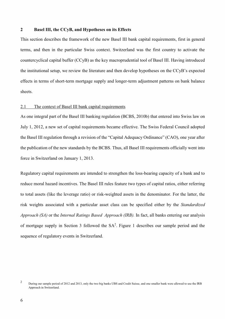
2 Basel III, the CCyB, and Hypotheses on its Effects
This section describes the framework of the new Basel III bank capital requirements, first in general
terms, and then in the particular Swiss context. Switzerland was the first country to activate the
countercyclical capital buffer (CCyB) as the key macroprudential tool of Basel III. Having introduced
the institutional setup, we review the literature and then develop hypotheses on the CCyB’s expected
effects in terms of short-term mortgage supply and longer-term adjustment patterns on bank balance
sheets.
2.1 The context of Basel III bank capital requirements
As one integral part of the Basel III banking regulation (BCBS, 2010b) that entered into Swiss law on
July 1, 2012, a new set of capital requirements became effective. The Swiss Federal Council adopted
the Basel III regulation through a revision of the “Capital Adequacy Ordinance” (CAO), one year after
the publication of the new standards by the BCBS. Thus, all Basel III requirements officially went into
force in Switzerland on January 1, 2013.
Regulatory capital requirements are intended to strengthen the loss-bearing capacity of a bank and to
reduce moral hazard incentives. The Basel III rules feature two types of capital ratios, either referring
to total assets (like the leverage ratio) or risk-weighted assets in the denominator. For the latter, the
risk weights associated with a particular asset class can be specified either by the Standardized
Approach (SA) or the Internal Ratings Based Approach (IRB). In fact, all banks entering our analysis
of mortgage supply in Section 3 followed the SA2. Figure 1 describes our sample period and the
sequence of regulatory events in Switzerland.
2 During our sample period of 2012 and 2013, only the two big banks UBS and Credit Suisse, and one smaller bank were allowed to use the IRB
Approach in Switzerland.
7
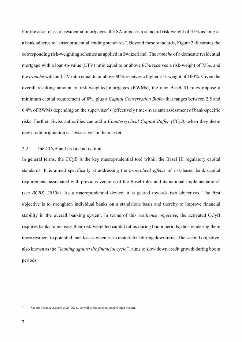
For the asset class of residential mortgages, the SA imposes a standard risk weight of 35% as long as
a bank adheres to “strict prudential lending standards”. Beyond these standards, Figure 2 illustrates the
corresponding risk-weighting schemes as applied in Switzerland. The tranche of a domestic residential
mortgage with a loan-to-value (LTV) ratio equal to or above 67% receives a risk-weight of 75%, and
the tranche with an LTV ratio equal to or above 80% receives a higher risk weight of 100%. Given the
overall resulting amount of risk-weighted mortgages (RWMs), the new Basel III rules impose a
minimum capital requirement of 8%, plus a Capital Conservation Buffer that ranges between 2.5 and
6.4% of RWMs depending on the supervisor’s (effectively time-invariant) assessment of bank-specific
risks. Further, Swiss authorities can add a Countercyclical Capital Buffer (CCyB) when they deem
new credit origination as "excessive" in the market.
2.2 The CCyB and its first activation
In general terms, the CCyB is the key macroprudential tool within the Basel III regulatory capital
standards. It is aimed specifically at addressing the procyclical effects of risk-based bank capital
requirements associated with previous versions of the Basel rules and its national implementations3
(see BCBS, 2010c). As a macroprudential device, it is geared towards two objectives. The first
objective is to strenghten individual banks on a standalone basis and thereby to improve financial
stability in the overall banking system. In terms of this resilience objective, the activated CCyB
requires banks to increase their risk-weighted capital ratios during boom periods, thus rendering them
more resilient to potential loan losses when risks materialize during downturns. The second objective,
also known as the “leaning against the financial cycle”, aims to slow down credit growth during boom
periods.
3 See for instance Aikman et al (2014), as well as the relevant papers cited therein.
8
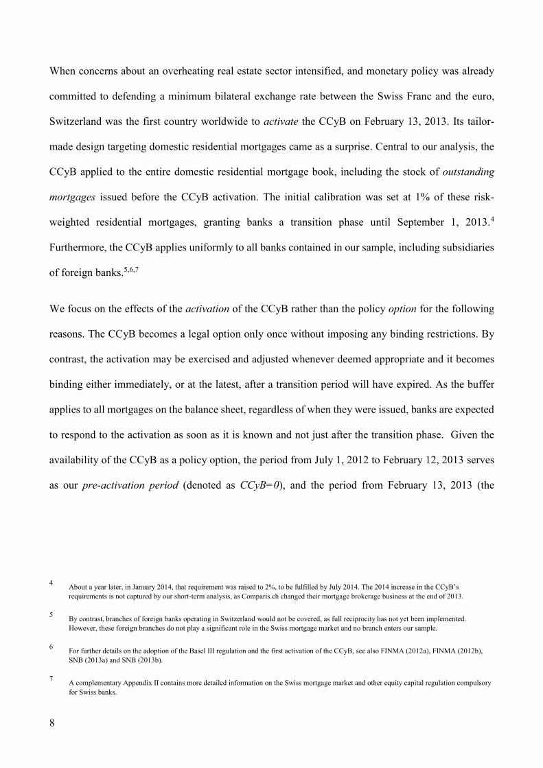
When concerns about an overheating real estate sector intensified, and monetary policy was already
committed to defending a minimum bilateral exchange rate between the Swiss Franc and the euro,
Switzerland was the first country worldwide to activate the CCyB on February 13, 2013. Its tailor-
made design targeting domestic residential mortgages came as a surprise. Central to our analysis, the
CCyB applied to the entire domestic residential mortgage book, including the stock of outstanding
mortgages issued before the CCyB activation. The initial calibration was set at 1% of these risk-
weighted residential mortgages, granting banks a transition phase until September 1, 2013.4
Furthermore, the CCyB applies uniformly to all banks contained in our sample, including subsidiaries
of foreign banks.5,6,7
We focus on the effects of the activation of the CCyB rather than the policy option for the following
reasons. The CCyB becomes a legal option only once without imposing any binding restrictions. By
contrast, the activation may be exercised and adjusted whenever deemed appropriate and it becomes
binding either immediately, or at the latest, after a transition period will have expired. As the buffer
applies to all mortgages on the balance sheet, regardless of when they were issued, banks are expected
to respond to the activation as soon as it is known and not just after the transition phase. Given the
availability of the CCyB as a policy option, the period from July 1, 2012 to February 12, 2013 serves
as our pre-activation period (denoted as CCyB=0), and the period from February 13, 2013 (the
4 About a year later, in January 2014, that requirement was raised to 2%, to be fulfilled by July 2014. The 2014 increase in the CCyB’s
requirements is not captured by our short-term analysis, as Comparis.ch changed their mortgage brokerage business at the end of 2013.
5 By contrast, branches of foreign banks operating in Switzerland would not be covered, as full reciprocity has not yet been implemented.
However, these foreign branches do not play a significant role in the Swiss mortgage market and no branch enters our sample.
6 For further details on the adoption of the Basel III regulation and the first activation of the CCyB, see also FINMA (2012a), FINMA (2012b),
SNB (2013a) and SNB (2013b).
7 A complementary Appendix II contains more detailed information on the Swiss mortgage market and other equity capital regulation compulsory
for Swiss banks.
9
activation of the tool), until the end of our dataset on October 24, 2013 is the post-activation period
(denoted as CCyB=1).
To avoid any distorting effects, our focus on the activation guarantees that pre- and post-activation
period are otherwise comparable, which would not be the case if we started our sample earlier. Also
on June 1, 2012 two additional changes in the Swiss mortgage market regulation became effective.
The Swiss Financial Market Supervisory Authority FINMA declared the Swiss Bankers Association’s
self-regulation as a new minimum standard applicable to all banks. First, Loan-to-Value (LTV) ratios
have to be reduced to at most two-thirds within at most 20 years after mortgage issuance.8 Second,
home buyers had to pledge at least 10% of the underlying property’s market value as “hard equity”,
i.e. in terms of own liquid funds while disregarding any pension-related assets.9,10
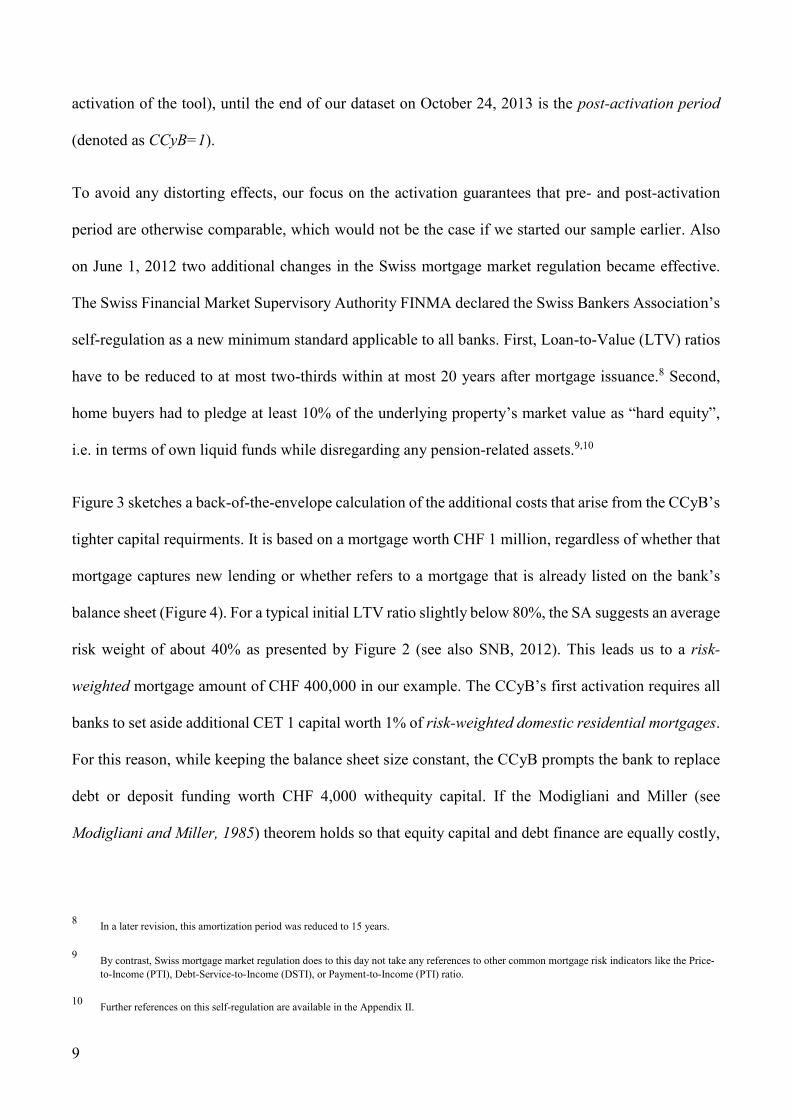
Figure 3 sketches a back-of-the-envelope calculation of the additional costs that arise from the CCyB’s
tighter capital requirments. It is based on a mortgage worth CHF 1 million, regardless of whether that
mortgage captures new lending or whether refers to a mortgage that is already listed on the bank’s
balance sheet (Figure 4). For a typical initial LTV ratio slightly below 80%, the SA suggests an average
risk weight of about 40% as presented by Figure 2 (see also SNB, 2012). This leads us to a risk-
weighted mortgage amount of CHF 400,000 in our example. The CCyB’s first activation requires all
banks to set aside additional CET 1 capital worth 1% of risk-weighted domestic residential mortgages.
For this reason, while keeping the balance sheet size constant, the CCyB prompts the bank to replace
debt or deposit funding worth CHF 4,000 withequity capital. If the Modigliani and Miller (see
Modigliani and Miller, 1985) theorem holds so that equity capital and debt finance are equally costly,
8 In a later revision, this amortization period was reduced to 15 years.
9 By contrast, Swiss mortgage market regulation does to this day not take any references to other common mortgage risk indicators like the Price-
to-Income (PTI), Debt-Service-to-Income (DSTI), or Payment-to-Income (PTI) ratio.
10 Further references on this self-regulation are available in the Appendix II.
10
the liability substitution imposed by the CCyB should not affect the bank’s total funding costs.11
However, if the Modigliani and Miller (1985) theorem fails, the bank has to bear the difference in
terms of funding costs. In our example, we thus multiply the extra capital requirement of CHF 4,000
with this cost differential, denoted as X. If that cost differential amounts to, for example, 10%, then the
CCyB will on average imply additional capital-related costs of CHF 400, or 4 basis points when set in
proportion to the requested total mortgage amount.12
2.3 Literature related to the CCyB
As Switzerland was the first country to activate the CCyB, empirical evidence on its immediate impact
and longer-term adjustment patterns is very scarce. A related stream of the literature investigates other
policy measures that share some specific features with the CCyB. Aiyar et al (2014a) evaluate the
effects of bank-specific capital requirements in the UK that used to vary counter-cyclically under Basel
I. They point out that, if there exists a set of lenders to whom such requirements do not apply, “policy
leakage” effects might ensue, which may defeat the purpose of countercyclical capital requirements.
The authors also find that the effectiveness of countercyclical capital requirements depends on banks’
existing levels of capitalization. In a parallel paper, Aiyar et al (2014b) study how shocks to minimum
capital requirements are transmitted internationally and they find a significantly negative effect on
cross-border lending. By contrast, Jiménez et al (2016) evaluate the effects of “dynamic provisioning”
– a measure introduced by the Spanish regulator in 2000.13 Using observations at the bank-loan-firm
11 Junge and Kugler (2013) find, for a sample of five publicly listed Swiss banks, that the elasticity between a bank’s leverage and its CAPM-β is
about 55% of what it would be if the Modigliani-Miller theorem did fully hold. Furthermore, in their analysis of the extra costs of Basel III, they
estimate a cost difference of 4.66% using the annual return of the Swiss SPI stock market index and the 12-month CHF LIBOR rate for 1990–2010.
12 While not relevant in the present case of a relatively small increase in capital requirements, in general X is possibly endogenous in that a stronger
capitalisation level will tend to reduce the bank’s overall risk profile and, hence, reduce the cost of other funding sources.
13 Crowe et al (2011) point out that countercyclical provisioning differs from countercyclical capital requirements in that provisioning requirements
can be binding also when banks are already better capitalized than required by regulators.
11
level, the authors analyze the impact of these provisions on bank lending to firms. They find that the
counter-cyclical provisioning rules did indeed help to smooth the Spanish credit cycle, even though
they failed to avert the build-up of vulnerabilities in the property sector. More recently, Auer and
Ongena (2016) also analyze effects of the CCyB in Switzerland. In distinct from our paper which is
focused on mortgage lending, they examine the impact on commercial lending, which was not
subjected to the CCyB and find some evidence of an increase in such lending.
Our paper also relates to the more general literature on the nexus between bank capitalization and bank
lending. On the theory side, Boot et al (1993), Sharpe (1990), and Diamond and Rajan (2000) develop
models that examine how changes to equity capital should affect bank lending. Gersbach and Rochet
(2012), in turn, show that the volatility of lending can be reduced by requiring higher capital ratios in
boom times. With respect to the regulatory framework, Repullo and Suarez (2004) investigate how the
transition from Basel I to Basel II translates into changes in a theoretical loan pricing equation. On the
empirical side, Kishan and Opiela (2000) stress that the degree of capitalization matters in that small
and less well capitalized banks respond most strongly to monetary policy. The impact of capital
cushions or “excess capitalization” is also investigated by Gambacorta and Mistrulli (2004 and 2014).
More specifically on the effects of regulatory capital requirements, several papers conduct mostly
accounting-based quantitative impact studies (QIS) on the effect of capital requirements on loan
pricing. These include King (2010), Cosimano and Hakura (2011) and Hanson et al (2011). Demir et
al (2014) find that the introduction of the Basel II standardized approach to risk weights in Turkey
affected real activity in the economy.
2.4 Hypotheses on the Effects of the CCyB
There are several possibilities for a bank to adjust to the CCyB’s additional capital requirements, both
over the short-term and over the longer term. Beyond the regulatory capital standards, Berger et al
(2008) present evidence that banks put aside so-called capital cushions which vary along the individual
12
bank’s risk preferences.14 Figure 5 illustrates these cushions for the pre- and the post-activation
periods. As an immediate effect, the CCyB activation shrinks the capital cushion and banks might
either prefer to accept a lower level in the long run, or restore the cushion over time.
To restore the cushion after the CCyB activation has consumed part of it, a bank can either target the
numerator of the envisaged new capital ratio by raising capital, or the denominator by constraining
the growth of its RWAs, or both, see Aiyar et al (2014)
The focus of our short-term analyses is on how banks adjust their mortgage supply. By rejecting more
applications, a bank can shrink the denominator. By raising prices, a bank can simultaneously gear the
numerator and denominator of its capital ratio: On the one hand, higher prices might (the more, the
less elastic demand) enable the bank to boost retained earnings and thereby to strengthen its capital
basis. On the other hand, higher prices might constrain new mortgage issuance (the more, the more
elastic demand).
The size of the cushion before higher capital requiments come into force matters. A bank which had
maintained a lower capital cushion might even see a capital shortfall if the additional capital
requirements imposed by the CCyB exceeded its cushion. Figure 6 reflects this situation for low-
cushion banks and their need to raise capital urgently.
The CCyB applies to both the stock of outstanding mortgages and new mortgage lending. For those
banks which operate a very mortgage-specialized business model, the CCyB implies a higher burden
in terms of additional capital requirements. Figure 7 shows that a higher burden absorbs more of the
potential capital cushion. Mortgages with longer remaining maturities will require relatively more
capital, for even longer time horizons which renders them even more costly. As rates on existing
14 Similar results are obtained for European banks by Jokipii and Milne (2011). They speak of “capital buffers”, while Berger et al speak of
“capital cushions” and Gambacorta and Mistrulli (2004) speak of “excess capital”. We follow Berger et al and speak of “capital cushions”.
13
mortgages cannot be adjusted,15 we expect that banks with a very mortgage-intensive business model
raise prices on new lending even more in order to cross-subsidize outstanding mortgages by passing
on the burden to new customers. The extent to which such cross-subsidization can be realized, depends
on the effective elasticity of the demand function faced by the individual bank. We hence hypothesize
that
Hypothesis 1
Banks that exhibit balance sheet characteristics that render them more sensitive to the regulatory
design of the CCyB, raise their mortgage rates relatively more in response to the CCyB’s tighter
capital requirements than their competitors. In particular,
a. relatively more capital-constrained banks with lower capital cushions and
b. banks which are relatively more specialized in the mortgage business, listing a higher stock
of outstanding mortgages with long-term remaining maturities on their balance sheets
… charge higher rates after the CCyB activation.
Furthermore, the additional CCyB-related capital requirements are determined by their stock of risk-
weighted domestic residential mortgages. Figure 7 illustrates how risk-weighting schemes translate the
individual customer’s loan-to-value (LTV) ratio, the credit risk of a borrower, into capital requirements
for a bank and thereby link the underlying borrower risk of a mortgage to the CCyB.16 In this way,
15 While some banks in Switzerland stipulate in loan contracts that they are also entitled to adjust fixed rates when regulatory costs change, doing
so in practice is reported to be difficult for reputational reasons.
16 Basel II implied a default risk weight of 35% for residential mortgages given “strict prudential lending standards” and mandated national authorities
to impose higher risk weights when such standards were not met. The risk-weighting scheme illustrated in Figure 3 reflects the Swiss
implementation of those more general principles applicable during our sample period. For details, see FINMA (2013a).
14
risk-weighting schemes put an extra capital levy on mortgages with LTV ratios equal to or above 67%,
and again on those with LTV ratios equal to or above 80%. We expect banks to claim extra
compensation for granting these more capital-consuming mortgages and even more so after the CCyB
imposes higher capital standards.17 This leads to our second hypothesis on the characteristics of
mortgage applicants.
Hypothesis 2
Risk-weighting schemes that are linked to the LTV ratio of a mortgage amplify the CCyB effect and
might trigger a relatively larger increase in mortgage rates for potential borrowers
with LTV ratios equal to or above 67%
and a yet larger increase for LTV ratios equal to or above 80%.
The focus of our longer-term analyses is on how banks adjust their capitalization, asset portfolio and
overall balance sheet structure in order to comply with the new overall capital requiments including
the CCyB. Higher rejection rates and higher prices will lower the pace of mortgage growth on bank
balance sheets. In the context of the Swiss mortgage market, this speaks to the “leaning against the
financial cycle”. Overall, mortgage lending might even decline and, thereby reduce the amount of risk-
weighted assets, and maybe even total assets at the bank-level, when keeping other asset classes
unchanged. The effects might again be stronger for banks with lower initial capital cushions and banks
with a specialization in the mortgage business. We hence expect that:
17 Higher credit risk is also implied by higher Price-To-Income (PTI) ratios. In our regressions, we implicitly control for PTI ratios.

15
Hypothesis 3
In the longer-term adjustment process, the response-level responses listed in Hypothesis 1 will
translate into changes on bank balance sheets. In this line of argument,
a. relatively more capital-constrained banks with lower capital cushions, and
b. banks which are relatively more specialized in the mortgage business, listing a higher stock
of outstanding mortgages with long-term remaining maturities
… will slow down their mortgage growth relatively more.
If banks succed in charging higher rates and passing on their burden to the customer, banks can
strenghten their capital basis by higher retained earnings. Raising corporate capital is more time
consuming and less likely to happen in the course of the subsequent months. Further, existing
shareholders prefer not to see the value of their shares decline by the bank issuing new shares. If all
banks adjust to the new capital standards including the CCyB by restoring their capital cushions, the
overall banking system will become more resilient and the first objective of the CCyB would be
achived. We hypothesize that
Hypothesis 4
Banks will strenghten their capital basis and restore their capital cushions in response to the CCyB.
As raising corporate capital is unlikely to happen over a few months, banks will most likely resort to
their accumulated profits or retained earnings to raise capital. Again the effect will be stronger for
those banks which had reported lower capital cushions and operated a more mortgage-focused
business model in the pre-activation period.

16
3 Short-term mortgage market response to the CCyB activation
3.1 Data
Unique features of the Comparis mortgage market dataset and bank characteristics
Our data on mortgage applications and bank responses were provided by the Swiss online platform
Comparis.ch. Comparis is a comparison website for various financial services including bank products,
health insurance plans, real estate markets and tax advice. Between 2008 and 2013, Comparis operated
a mortgage brokerage that allowed households to submit personalized mortgage applications in order
to receive different binding quotes from participating lenders.18 To access the service and compare
offers, customers paid CHF 148 (about USD 150) and gave comprehensive information on the property
to be bought, the requested mortgage amount, the desired maturity model, household finances, and
personal details such as their age. Comparis then sent the anonymized request to different lenders,
including banks from all major banking groups, except for the two big banks UBS and Credit Suisse
(CS).1920 After having assessed the customer’s financial situation, mortgage lenders decided whether
to make a binding offer and at which mortgage rate and conditions. While banks were allowed to split
the mortgage into different tranches with tranche-specific rates, they were not allowed to deviate from
the requested amount in total.
The Comparis dataset forms the backbone of our paper and it has several remarkable features that suit
our empirical approach. First, it allows us to disentangle mortgage demand and supply, as we observe
how different banks respond to the same mortgage application with customer-specific features. Such
18 Comparis has changed its mortgage platform and business model significantly in late 2013. Since then, customers pre-select from a list of lenders
and discuss their needs with an advisor before receiving offers from different lenders. The period for which we have data ends with the end of the previous business model on October 24, 2013.
19 UBS and CS are also the only ones computing their risk weights with the Internal Ratings Based (IRB) approach rather than the Standardized
Approach (SA), which has changed during the sample period. All other banks in our sample homogeneously use the SA.
20 Three insurance companies also offered mortgages via Comparis. We do not include them in this analysis, as we lack information on their
balance sheets.
17
a comparison of multiple lenders per borrower is typically available from the syndicated loan market
for corporate or interbank lending, or if a country maintains a credit register. Those datasets provide
information on contracted loans, whereas our data is collected at the application-response-level, hence,
before signing a mortgage contract. As Comparis sent the customer-specific data to all participating
lenders without asking for a deliberate choice by applicants, we can rule out any potential self-selection
of customers into different types of banks. Second, we are able to observe both the willingness to make
a loan (like Jiménez et al, 2012) and comprehensive details on the pricing of the mortgage including
tranche-specific rates by maturity and borrower risk as assessed by the potential lender. Third, all
lenders receive the same anonymized information, which rules out that they could take advantage of
additional soft information, considerations of relationship lending or cross-selling of products.
Furthermore, we observe exactly the same set of detailed information that banks receive, so banks
cannot act on any information that we would not be able to control for. Fourth, lenders do neither know
which competitors are participating, nor which rates they are offering. These features warrant that
lenders submit binding, independent offers that truly reflect their eagerness to bid for the mortgage.
Fifth, the customer incurs a fee on submitting his application and, as offers are binding conditional on
verifiable information, they have an incentive to submit correct information.
Bank-level data for participating banks
We complement the Comparis dataset with supervisory reports from the Swiss Financial Market
Supervisory Authority (FINMA). Bank-level data of the 21 participating lenders help us to analyze
how their CCyB response in the mortgage market varies with their reported capitalization, their asset
portfolio and other balance sheet characteristics before the activation. To measure capitalization, we
focus on Core Equity Tier 1 (CET 1) as a percentage of risk-weighted assets (RWA). Specifically, our
empirical analysis draws on the “capital cushion”, defined as the reported level of capital
(CET1/RWA) that a bank holds in excess of the regulatory requirements to be fulfilled by the end of
the Basel III transition period. As a measure of mortgage market specialization, we use the share of
18
mortgages with a remaining maturity of at least 5 years relative to a bank’s total assets. To isolate the
effects of capitalization and specialization, we control for other time-varying balance sheet
characteristics like the banks’ funding model, liquidity, size and recent month-on-month mortgage
growth.
Demand and Supply before and after the CCyB Activation
Table 1 introduces our Comparis dataset in terms of demand and supply. The first column refers to the
period CCyB=0 starting on July 1, 2012, while the second column ranges from the activation of the
CCyB on February 13, 2012, until the end of our sample on October 24, 2013 (CCyB=1). Our data on
mortgage demand shows that the number of applications per months remains relatively constant over
both periods. Turning to mortgage supply, Table 1 shows that customers receive on average 4.2
(=4509/1075) answers in the period before the CCyB activation and 3.6 (=3507/983) answers after it.
More importantly, the shares of offers and rejections relative to the total number of answers is almost
stable. On average, 86% of all received responses are offers before the activation of the CCyB and
85% after it. This mitigates potential selection concerns in that banks might constrain their lending by
rejecting more applications after the CCyB went into force. We will return to various types of potential
selection biases below.
The structure of our dataset is unique in that it allows us to follow a very clean identification strategy
at the mortgage-response-level. Unfortunately, we cannot observe which offer the customer ultimately
chooses and hence, we can only draw inferences on new mortgage lending based on the cheapest
quotes that the customer is most likely to accept. The question then arises whether this dataset is
actually representative of the entire Swiss mortgage market. In Section 4, we examine how banks
adjust their capitalization, mortgage lending and overall balance sheet structure in the longer run. It
draws on the full sample of all banks chartered in Switzerland and provides findings that are consistent
with our short-term mortgage market response based on a subsample of the banking population.
19
Further, Appendix II offers a host of comparisons and tests based on publicly available statistics on
the entire Swiss mortgage market. These analyses confirm that the data are representative, both in
terms of the mortgage demand (geographical distribution, borrower risk, etc.) and supply.
One might also raise the concern that the CCyB impacts mortgage demand and supply in terms of the
submitted and accepted borrower risk profiles. As a simple first step, Table 2 presents simple T-tests
to address this issue. With respect to mortgage demand, customers might expect banks to reject more
requests with high loan-to-value (LTV) ratios and therefore shy away from requesting riskier
mortgages in the first place. If that was the case, our analyses of mortgage rates might suffer from a
selection bias, as fewer risky mortgages would enter the sample after the CCyB activation. The
Mortgage Demand panel of Table 2 shows that in the full sample, neither applicants’ LTV nor PTI
ratios change significantly across periods. We then split our sample into customers asking for a new
mortgage and customers requesting to roll over their outstanding mortgage with a new bank. Our
results suggest that there is no significant difference in the borrower risks profiles for new customers.
Only the requested LTV ratios for rollover requests decline slightly after the activation of the CCyB.
For this reason, our more sophisticated empirical analysis in Section 3 will distinguish between
rollover and new mortgage applications and control for different types of borrower risk.
With respect to mortgage supply, the second panel of Table 2 confirms our previous finding that the
share of offers remains constant over timer. We conclude that banks do not constrain lending by
rejecting more applications. We infer from this finding, that any CCyB effect should operate through
the pricing of mortgages. The remainder of Table 2 provides evidence for these significant differences
in the pricing of all mortgages across activation periods. However, simple t-tests can neither
accommodate the complexity of our mortgage pricing data, nor can they account for any concomitant
macro factors. The next sub-sections offers more sophisticated regression specifications to gain more
detailed insights.
20
3.2 Empirical Analysis: Which banks are most sensitive to the CCyB activation?
Empirical Strategy
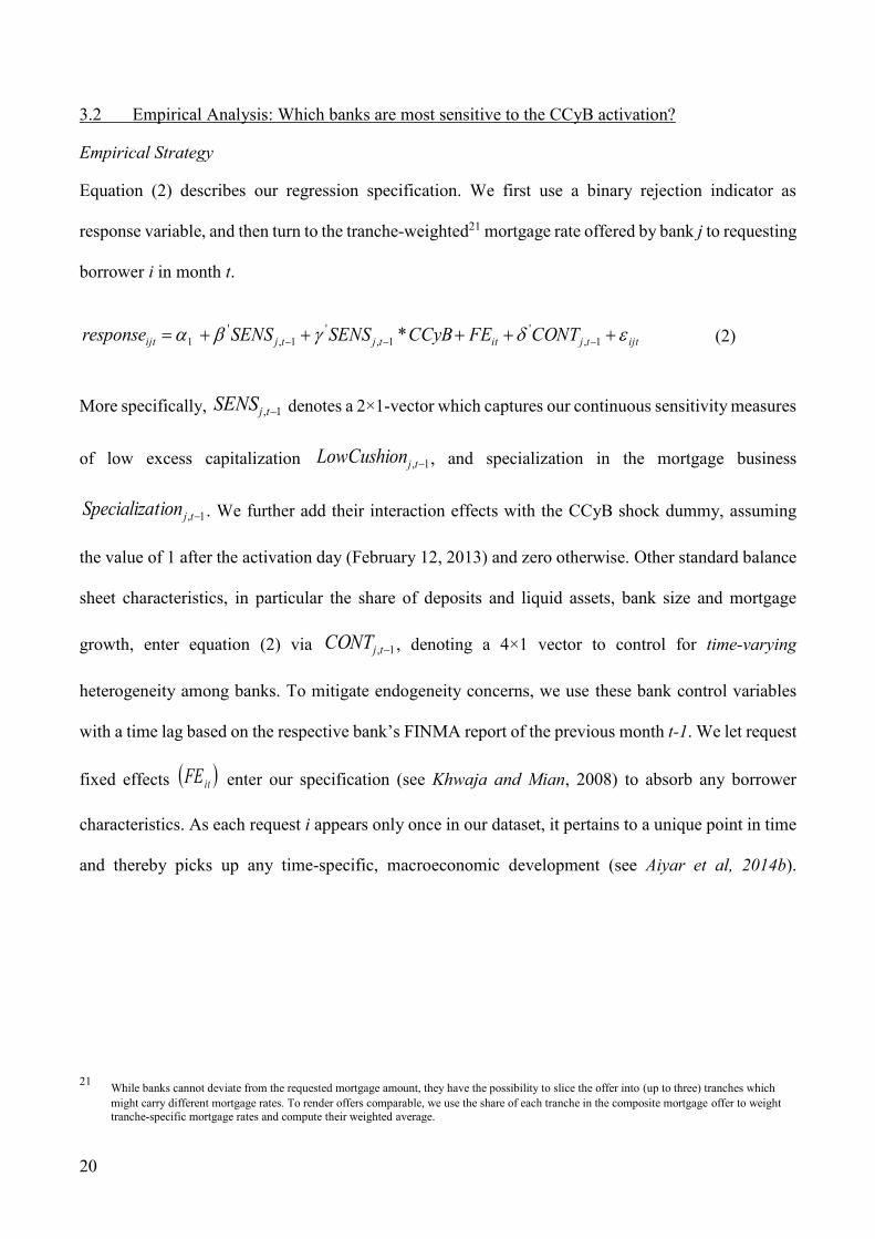
Equation (2) describes our regression specification. We first use a binary rejection indicator as
response variable, and then turn to the tranche-weighted21 mortgage rate offered by bank j to requesting
borrower i in month t.
ijttjittjtjijt CONTFECCyBSENSSENSresponse 1,
'
1,
'
1,
'
1 * (2)
More specifically, 1, tjSENS denotes a 2×1-vector which captures our continuous sensitivity measures
of low excess capitalization 1, tjLowCushion , and specialization in the mortgage business
1, tjtionSpecializa . We further add their interaction effects with the CCyB shock dummy, assuming
the value of 1 after the activation day (February 12, 2013) and zero otherwise. Other standard balance
sheet characteristics, in particular the share of deposits and liquid assets, bank size and mortgage
growth, enter equation (2) via 1, tjCONT , denoting a 4×1 vector to control for time-varying
heterogeneity among banks. To mitigate endogeneity concerns, we use these bank control variables
with a time lag based on the respective bank’s FINMA report of the previous month t-1. We let request
fixed effects itFE enter our specification (see Khwaja and Mian, 2008) to absorb any borrower
characteristics. As each request i appears only once in our dataset, it pertains to a unique point in time
and thereby picks up any time-specific, macroeconomic development (see Aiyar et al, 2014b).
21 While banks cannot deviate from the requested mortgage amount, they have the possibility to slice the offer into (up to three) tranches which
might carry different mortgage rates. To render offers comparable, we use the share of each tranche in the composite mortgage offer to weight
tranche-specific mortgage rates and compute their weighted average.
21
Standard errors are clustered by bank and activation period to obtain a reasonable number of clusters
with a relatively balanced number of observations per cluster.22,23
Capital-Constrained Banks with low capital cushions (Hypothesis 1a)
First, we examine the role of low capital cushions, defined as the negative, percentage point deviation
of a bank’s reported capital ratio (total capital as a percentage of risk-weighted assets) from the capital
ratio below which the supervisor would intervene.24 ,25, Banks with more comfortable capital cushions
dispose of more degrees of freedom, but they might also charge higher prices to preserve their
cushions. On the flip side, banks with lower capital cushions might pursue more aggressive pricing
strategies 01 . Yet, once the CCyB imposes an additional capital charge, these banks become
relatively more constrained, and for this reason, they might reject more mortgage applications. In case
of submitting an offer, we assume that banks with lower capital cushions most likely charge higher
rates as a compensation for granting a mortgage 01 in an attempt to boost their profits and
ultimately to bolster their capital position.
Specialized banks with mortgage-intensive business models (Hypothesis 1b)
Specialization in the mortgage business, defined as the total asset share of mortgages with a remaining
maturity of 5 years and beyond, might render a bank more sensitive to the CCyB’s particular Swiss
design. These banks benefit from economies of scale and they might pass on part of those to their
customers by charging lower mortgage rates 02 , on average. Another possibility might be that
22 See Wooldridge (2003) or Petersen (2009) for a general discussion on the computation of standard errors in finance panel datasets.
23 As a robustness check, we use robust standard errors and cluster them by request. Our results remain virtually unaffected.
24 As distinct from the previous section and Figures 5-7, we believe that it is more intuitive to use the “low capital cushion” measure, inversely
defined, as this suits the idea that more capital-constrained banks charge higher prices.
25 The intervention threshold in Switzerland differs across five risk categories, into which the supervisor has allocated banks depending on amongst
others a bank’s total assets.
22
they lack diversification and hence add a premium to their mortgage rates in which case we might find
that 02 . After the activation, we expect more specialized banks to reject more applications, as
the CCyB applies to all residential mortgages listed on balance sheets. Given that specialized banks
submit an offer, they most likely raise their rates substantially 02 as their mortgage portfolio
consumes a higher share of their capital.
Descriptive Statistics
Table 3 reports the descriptive statistics for the Comparis estimation sample. Panel A refers to our
binary rejection analysis, while Panel B draws on the analysis of mortgage pricing. A difference in the
number of observations emerges from the fact that we drop all rejections in Panel B. This might also
give rise to a slightly different weighting scheme of borrower and lender characteristics when
computing summary statistics. The average LTV ratio hovers around 64% in both panels. About 55% of
all submitted LTV ratios in Panel A (and 56% in Panel B) equal to or exceed 66%. The average offer is
sent to an applicant aged about 46 years, who reports an average annual household income of CHF 181,000
(about USD 181,000) and average household wealth, including retirement savings, worth about CHF
507,000 (about USD 507,000). With respect to the participating bank’s balance sheet setup, Panel A and B
reveal hardly any difference. Banks set aside capital cushions between 0.5% and 12% of risk-weighted
assets during the sample period. Our measure of bank specialization in the mortgage business, the
outstanding stock of mortgages with residual maturity of 5 years or longer, ranges between 7 % and 22%
of total assets.
Bank Sensitivity Measures: Results
Table 4 tells us whether more sensitive banks reject more applications after the CCyB activation, while
Tables 5 and 6 analyze their pricing behavior to provide formal tests of Hypotheses 1a and 1b. In each
table, Column 1 refers to the full sample of mortgage requests, Columns 2-5 isolate requested fixed
rate mortgages (FRMs) with Columns 3- 5, in turn, splitting those by distinct requested fixed term
23
maturities26 spanning 10 years, 5 to 10 years, and 5 years. According to the information provided by
the applicant, Columns 6 and 7 distinguish between different types of borrower risk, and Columns 8
and 9 separate requests for new mortgages from rollover requests.
Our results in Table 4 suggest that banks with a lower capital cushion are less likely to reject a mortgage
in general, however this equally holds before and after the CCyB activation. Sample splits reveal that
this result is driven by medium-term maturity mortgages, mortgages with higher credit risk and new
mortgage applications. Table 4 further suggests that the degree of bank specialization in the mortgage
business does not shape its accept-reject decision – again, independent from the period under
consideration. These results align well with Edelberg (2006) in that banks prefer to attract or discard
a customer along the price dimension rather than by sending outright rejections. As Table 4 does not
provide any evidence for a change in the rejection behavior over time, we can safely refute any
concerns about selection biases and proceed to the analysis of mortgage pricing.
Our results in Table 5 point out that more capital-constrained banks with lower capital cushions raise
their rates relatively more after the CCyB than their less constrained peers. Fixed rate mortgage (FRM)
models, while accounting for more than 80% of all our observations, especially those with a 10y
maturity (making up almost 60% of the entire sample), drive this result. After the CCyB activation,
banks with lower capital cushions charge on average 72 bps more for a 10y fixed rate mortgage which
reflects their tradeoff between hitting the now even closer capital requirement threshold and reaping
additional profits. Before the activation period, Table 5 shows that less well capitalized banks had on
average submitted cheaper offers. Remarkably, we do not find a significant interaction effect for the
sub-sample of requests with higher LTV ratios or credit risk, as the risk-weighting schemes for those
26 This list of mortgage models that customers can request is not exhaustive. Fixed rate mortgages are available for each annual maturity between 1
and 10 years apart from different models of adjustable rate maturities. We focus on longer-term fixed rate models here as we expect an
immediate effect on the bank’s rejection and pricing behavior to be observable as those mortgages would be part of their balance sheet after the
transition period ending in September 2013 and the CCyB becomes binding. Columns 6 -10 refer to all mortgage maturity models.
24
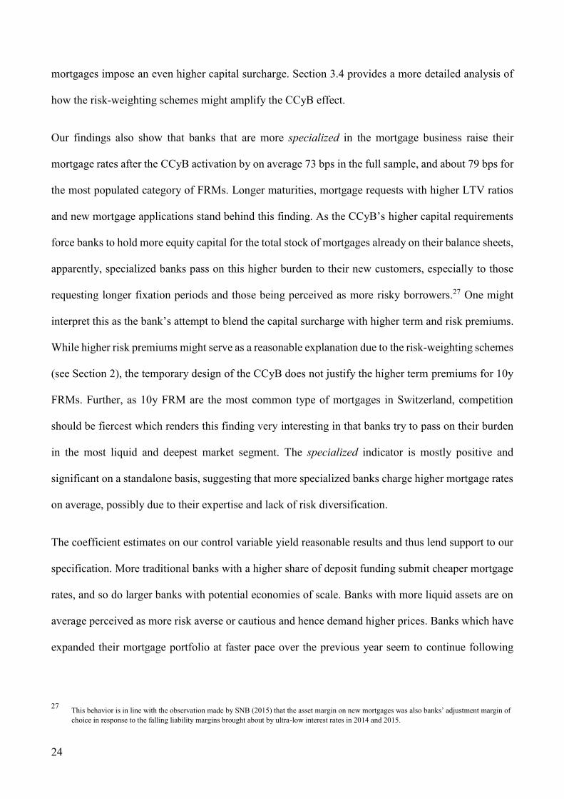
mortgages impose an even higher capital surcharge. Section 3.4 provides a more detailed analysis of
how the risk-weighting schemes might amplify the CCyB effect.
Our findings also show that banks that are more specialized in the mortgage business raise their
mortgage rates after the CCyB activation by on average 73 bps in the full sample, and about 79 bps for
the most populated category of FRMs. Longer maturities, mortgage requests with higher LTV ratios
and new mortgage applications stand behind this finding. As the CCyB’s higher capital requirements
force banks to hold more equity capital for the total stock of mortgages already on their balance sheets,
apparently, specialized banks pass on this higher burden to their new customers, especially to those
requesting longer fixation periods and those being perceived as more risky borrowers.27 One might
interpret this as the bank’s attempt to blend the capital surcharge with higher term and risk premiums.
While higher risk premiums might serve as a reasonable explanation due to the risk-weighting schemes
(see Section 2), the temporary design of the CCyB does not justify the higher term premiums for 10y
FRMs. Further, as 10y FRM are the most common type of mortgages in Switzerland, competition
should be fiercest which renders this finding very interesting in that banks try to pass on their burden
in the most liquid and deepest market segment. The specialized indicator is mostly positive and
significant on a standalone basis, suggesting that more specialized banks charge higher mortgage rates
on average, possibly due to their expertise and lack of risk diversification.
The coefficient estimates on our control variable yield reasonable results and thus lend support to our
specification. More traditional banks with a higher share of deposit funding submit cheaper mortgage
rates, and so do larger banks with potential economies of scale. Banks with more liquid assets are on
average perceived as more risk averse or cautious and hence demand higher prices. Banks which have
expanded their mortgage portfolio at faster pace over the previous year seem to continue following
27 This behavior is in line with the observation made by SNB (2015) that the asset margin on new mortgages was also banks’ adjustment margin of
choice in response to the falling liability margins brought about by ultra-low interest rates in 2014 and 2015.
25
that strategy by underbidding their competitors’ prices. A robustness check below discusses whether
these expansionary banks switch strategies after the CCyB activation.
In brief, we find evidence consistent with Hypotheses 1a and 1b that capital-constrained as well as
mortgage-specialized banks raise their mortgage rates relatively more. We infer that the composition
of mortgage supply changes in that banks with a higher exposure to the CCyB’s regulatory design
substantially adjust their mortgage pricing. We highlight these two results as core findings of our paper.
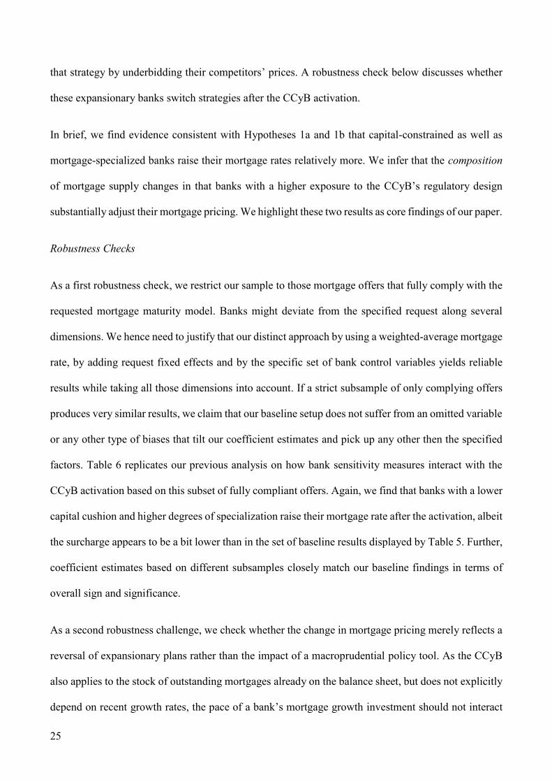
Robustness Checks
As a first robustness check, we restrict our sample to those mortgage offers that fully comply with the
requested mortgage maturity model. Banks might deviate from the specified request along several
dimensions. We hence need to justify that our distinct approach by using a weighted-average mortgage
rate, by adding request fixed effects and by the specific set of bank control variables yields reliable
results while taking all those dimensions into account. If a strict subsample of only complying offers
produces very similar results, we claim that our baseline setup does not suffer from an omitted variable
or any other type of biases that tilt our coefficient estimates and pick up any other then the specified
factors. Table 6 replicates our previous analysis on how bank sensitivity measures interact with the
CCyB activation based on this subset of fully compliant offers. Again, we find that banks with a lower
capital cushion and higher degrees of specialization raise their mortgage rate after the activation, albeit
the surcharge appears to be a bit lower than in the set of baseline results displayed by Table 5. Further,
coefficient estimates based on different subsamples closely match our baseline findings in terms of
overall sign and significance.
As a second robustness challenge, we check whether the change in mortgage pricing merely reflects a
reversal of expansionary plans rather than the impact of a macroprudential policy tool. As the CCyB
also applies to the stock of outstanding mortgages already on the balance sheet, but does not explicitly
depend on recent growth rates, the pace of a bank’s mortgage growth investment should not interact
26
with the CCyB effect per se. We would expect that banks pursuing an ambitious mortgage growth
strategy submit cheaper rates 0m on average. However, if at some point in time they decide to
reverse their strategy, we might see the overall price effect losing its significance or switching signs
(if the interaction effect was positive and significant, we would use an F-test to assess the overall
pricing effect as the sum of standalone plus the interaction coefficients: mm ). Our empirical tests,
however, reveal that banks exhibiting strong mortgage growth do not scale back their expansion plans
after the CCyB’s activation. We hence conclude that our baseline coefficient estimates reflect a policy
implication instead of accidentally picking up a concomitant reversal in business strategies.
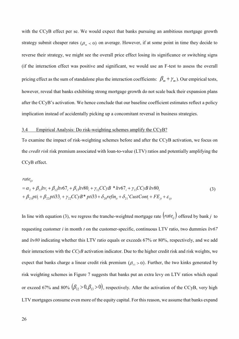
3.4 Empirical Analysis: Do risk-weighting schemes amplify the CCyB?
To examine the impact of risk-weighting schemes before and after the CCyB activation, we focus on
the credit risk risk premium associated with loan-to-value (LTV) ratios and potentially amplifying the
CCyB effect.
ijtjtiitii
iiiii
ijt
FECustContrefinptiCCyBptipti
ltvCCyBltvCCyBltvltvltv
rate
'33*33
8067*8067
2120222221
13121312112 (3)
In line with equation (3), we regress the tranche-weighted mortgage rate ijrate offered by bank j to
requesting customer i in month t on the customer-specific, continuous LTV ratio, two dummies ltv67
and ltv80 indicating whether this LTV ratio equals or exceeds 67% or 80%, respectively, and we add
their interactions with the CCyB activation indicator. Due to the higher credit risk and risk weights, we
expect that banks charge a linear credit risk premium 011 . Further, the two kinks generated by
risk weighting schemes in Figure 7 suggests that banks put an extra levy on LTV ratios which equal
or exceed 67% and 80% 0,0 1312 , respectively. After the activation of the CCyB, very high
LTV mortgages consume even more of the equity capital. For this reason, we assume that banks expand
27
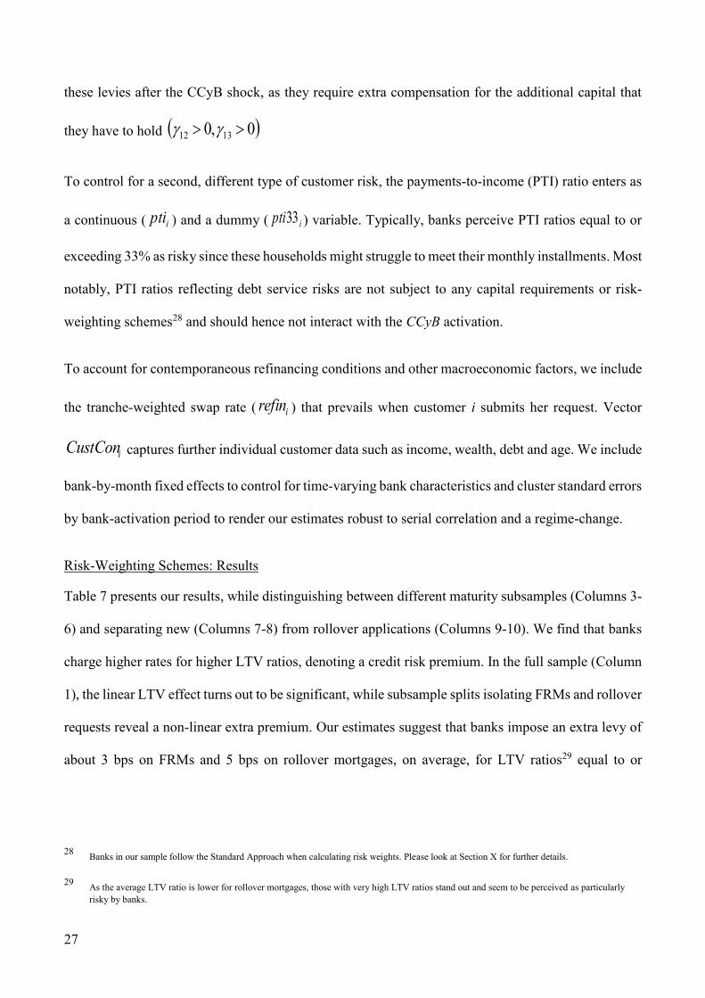
these levies after the CCyB shock, as they require extra compensation for the additional capital that
they have to hold 0,0 1312
To control for a second, different type of customer risk, the payments-to-income (PTI) ratio enters as
a continuous ( ipti ) and a dummy ( ipti33 ) variable. Typically, banks perceive PTI ratios equal to or
exceeding 33% as risky since these households might struggle to meet their monthly installments. Most
notably, PTI ratios reflecting debt service risks are not subject to any capital requirements or risk-
weighting schemes28 and should hence not interact with the CCyB activation.
To account for contemporaneous refinancing conditions and other macroeconomic factors, we include
the tranche-weighted swap rate ( irefin ) that prevails when customer i submits her request. Vector
iCustCon captures further individual customer data such as income, wealth, debt and age. We include
bank-by-month fixed effects to control for time-varying bank characteristics and cluster standard errors
by bank-activation period to render our estimates robust to serial correlation and a regime-change.
Risk-Weighting Schemes: Results
Table 7 presents our results, while distinguishing between different maturity subsamples (Columns 3-
6) and separating new (Columns 7-8) from rollover applications (Columns 9-10). We find that banks
charge higher rates for higher LTV ratios, denoting a credit risk premium. In the full sample (Column
1), the linear LTV effect turns out to be significant, while subsample splits isolating FRMs and rollover
requests reveal a non-linear extra premium. Our estimates suggest that banks impose an extra levy of
about 3 bps on FRMs and 5 bps on rollover mortgages, on average, for LTV ratios29 equal to or
28 Banks in our sample follow the Standard Approach when calculating risk weights. Please look at Section X for further details.
29 As the average LTV ratio is lower for rollover mortgages, those with very high LTV ratios stand out and seem to be perceived as particularly
risky by banks.
28
exceeding 66%. These coefficient estimates reflect the first kink at LTV ratios of 66%, associated with
risk-weighting schemes and additional capital requirements in Figure 7. The second kink at 80% turns
out to be insignificant.
Most central to the risk-weighting schemes, we find that the interaction effects of the CCyB activation
dummy with LTV indicators turn out to be insignificant which shows that risk-weighting schemes do
not amplify the CCyB effect. This result holds for new as well as rollover mortgages, and it is also
confirmed across all subsample estimations by maturity model. Given that escalating risk weighs only
apply to the tranches exceeding LTV ratios of 66% and 80%, respectively, instead of the entire
mortgage, the additional capital that banks need to hold for high-LTV mortgages does apparently not
induce them to expand the levy after the CCyB activation.
We stress this as the second core finding of our paper, while rejecting Hypothesis 2. One interpretation
of this finding might be that LTV threshold indictors just set apart riskier mortgages, inducing lenders
to charge a credit risk premium. In that case, risk-weighting schemes might indeed prove to be
ineffective when capital requirements on behalf of the bank become stricter, while lending standards
with respect to the customer risk characteristics in general remain unaffected.
Related to PTI ratios as a proxy for a different kind of borrower risk, we find differential effects for
new and rollover mortgages. Banks charge extra for new mortgages in proportion to their reported PTI
ratios, but not for rollover mortgages. Indeed, the linear PTI effect on rollover mortgage is slightly
negative, but dwarfed by the extra premium that banks impose on very high LTV ratios.
As the CCyB’s design only captures higher LTV ratios, we challenge our results by also looking at the
interaction effects with high PTI indicators. Given that customer risk is sanctioned only by tighter
capital requirements in terms of credit risk, but not in terms of debt service risk, one might image that
banks extend more lending to high PTI customers. Our results, however, do not support such a
substitution effect.

29
We now briefly discuss our results on control variables in Columns (1) to (5) in order to assess whether
our regression specification overall yields reasonable results. The estimated coefficient on the swap
rate states that a 100 bps increase in the swap rate translates into an increase of the average mortgage
rate of about 77 bps. A hint at the fact that many of our participating banks substantially draw on retail
instead of wholesale funding can rationalize this number. We further find that a one percentage point
increase in the customer’s income reduces the offered mortgage rate by up to 4 basis points. Banks
charge lower mortgage rates for customers with higher specified levels of wealth requesting FRM and
new mortgages and give a discount for older customers in the full sample.
We conclude from these results that LTV thresholds do not amplify the CCyB effects for banks, which
hints at the weak nexus between risk-weighting schemes and capital requirements. However, it is still
possible that a signaling mechanism is at work. If the aggregate risk perception for all mortgages has
surged, but not for riskier ones in particular, our time fixed effects would absorb the effect.
Robustness Checks
To challenge our findings, we again isolate those offers which offer a fully compliant mortgage
maturity. Our results turn out to be robust with only slight deviations in terms the size of coefficient
estimates.
Another concern might be that banks become in general more risk averse after the CCyB activation
and rise their risk premiums on average. As the interactions effect with both indicators of borrower
risk, credit risk and debt service risk reveal to be insignificant, we can also safely reject this concern.
30
4 Analysis of Balance Sheet Adjustments using Supervisory Data on all Swiss Banks
In this section, we investigate how the differential price increases at the response-level have affected
banks' overall balance sheets and capitalization in the months after the activation. To do so, we start
with supervisory bank balance sheet data covering not only the Comparis sample, but all banks
chartered in Switzerland.
Data
Starting with all Swiss banks, we focus on the subsample of retail banks in order to compare their
adjustments with those shown by banks in our Comparis sample.30 Based on banking groups as defined
by FINMA, we refer to retail banks as those banks whose balance sheet effective activities account for
earn at least 85% of their income, i.e. as net interest income, as opposed to fees and commissions31.
Table 9 shows summary statistics of our variables for the pre- and the post-activation periods and it
provides T-tests to compare how averages evolve over time. The top panel describes all retail banks
used for our baseline analyses in this section, while the bottom panel draws on the Comparis sample
as analyzed in the previous section. Our restrictive retail bank sample contains 36 banks, observed
over 14 months (January 2012 – February 2013, a total of 504 monthly observations) before and 10
months (March 2013 – December 2013, 360 observations) after the CCyB activation. Core Equity Tier
1 (CET1) capital and Risk-Weighted Assets (RWA), as well as all variables building on those, are
observed only at quarterly frequency32. The first rows show our two bank sensitivity measures, capital
30 By contrast, focusing the bank level analyses even more narrowly only on the 21 banks contained in the Comparis sample would not yield
enough observations.
31 The latter are more relevant for Switzerland's many wealth management banks, and trading income. As a robustness check, we include also
banks with interest income accounting for 55-85% of total income, as well as "universal" banks with interest income below 55%, fee income below 55%, and trading income below 20% of total income.
32 We assign missing values to those periods in which the underlying value was either zero or missing, and to periods in which absolute growth
rates equaled or exceeded 100% to avoid distorting our sample by capturing complete sell-offs or new acquisition of a portfolio that would
typically occur as part of a merger.
31
cushion and specialization. They are followed by the bank-level controls used in our response-level
analyses, and then we turn to other variables as analyzed in this section. Within the set of adjustment
variables, for all fractions we display the year-on-year difference in percentage points and for all other
variables the year-on-year percentage growth rate.
Against the regulatory requirements to be satisfied by the end of the Basel III phase-in period (2019),
retail banks report a CET1 capital cushion worth 7.99% of RWA over the pre-activation period,
compared to the economically similar value of 6.09 for Comparis banks. Capital cushions for both
groups contract in the second period, when requirements increase, however, for the average bank none
of these contractions is statistically significant.
Before the CCyB activation, specialization in the mortgage business, measured as the share of
outstanding long-term mortgages maturing in 5 years or beyond, amounts to about 10.8% of total assets
for the average retail bank, and to about 11.8% for the average bank in the Comparis sample. Over the
post-activation period, these shares rose significantly by more than 3 percentage points, respectively.
These outcomes seemingly contrast with the intended effects, and deserve some closer investigation.
Of course, averages as displayed in Table 9 mask the heterogeneinity across banks and their differential
sensitivities to the CCyB's design. For this reason, we argue that only our regression approach in
Section 3 can disentangle differential adjustment patterns, while revealing a change in the overall
composition of mortgage supply.
Our regression analyses below draw on annual growth rates and absolute changes. Looking at our
outcome variables of interest, we see that the annual growth rate of CET1 capital increased from about
3% to about 6% in both sets. The average retail bank kept its pace of RWA expansion almost stable
(the change is actually insignificant), such that the average annual change in capitalization ratios
CET1/RWA rose significantly by 0.3 percentage points. In parallel, the average Comparis bank
reduced the pace of RWA growth and strengthened its capital ratio significantly, resulting in a 0.5
32
percentage point rise in the year-on-year changes in the ratio of CET1 over RWA. Based on these
facts, we infer that the sample of retail banks mirrors the behavior that of the Comparis subset and vice
versa. In our empirical analysis below, we can hence resort to the broader sample of retail banks with
more observations to yield some meaningful results.
Empirical Approach
To identify the effects of the CCyB on bank balance sheets, we apply a Difference-in-Difference (DiD)
approach. We compare changes in the outcomes of interest between the pre- and post-CCyB periods
and across banks with different a priori levels of capital cushions and mortgage specialization. This
leads to the following estimation:
jjjt tionSpecializaCCyBLowCushionCCyBoutcome ** 21
jtjj tionSpecializaLowCushionCCyB 543 (4)
For our baseline estimations, we use only these basic DiD regressors. Robustness analyses with bank-
level controls or bank and time fixed effects yield similar results and are available on request.
Results
Table 10, Column 1 shows that the analyzed effects on mortgage pricing in Section 2 do indeed
translate into differential changes in mortgage growth: More specialized banks, while expanding their
mortgage business year-on-year during the pre-activation period, reduce their pace by 0.19 percentage
points after the activation. This finding is statistically significant at the 1% level, while clustering
standard errors by bank to account for serial correlation. By contrast, banks with a relatively lower
capital cushion were already trimming their mortgage lending before the CCyB activation and even
more so after it. However, none of these estimates is significant at the conventional levels when
33
clustering by bank. Instead of scaling back the mortgage business, banks with lower capital cushions
significantly reduced their growth rates in interbank lending.
Our effects are economically significant and remarkable, as retails banks actually expanded their
mortgage portfolio by almost 3% year-on-year before the CCyB activation, and accelerated the annual
pace by 2.4 percentage points during the post CCyB activation period, on average.. These results point
to a significant change in the composition of mortgage supply. New mortgage issuance shifted away
from very specialized banks with higher volumes of long-term mortgages on balance sheets and those
with lower capital cushions to those banks less specialized and more resilient in terms of capitalization.
Table 10 also shows that the overall expansion of retail banks in the mortgage business contrasts with
a general trend during the post-activation period. Column 2 suggests that banks significantly cut back
on lending to all sectors during this time. The 16 percentage point decline must hence be driven by
other business segments, like lending to the non-bank corporate sector. Before the activation, banks
reported strong annual growth rates of overall loan issuance reaching 14%, on average.
When turning to the liability side, we find that more specialized banks actually reversed their funding
strategies across periods. Before the activation, they had increasingly relied on deposit and bond
funding, covered bond funding in particular. Our estimates for the post CCyB period reveal that, they
revised their funding patterns and raised more equity capital. Due to a lack of significance, we do not
elaborate on the funding strategies of low cushion banks.
Table 11 analyzes the effects on capitalization in more detail. Here, we focus specifically on Core
Equity Tier 1 (CET1) capital, in which the CCyB requirements are specified. Column 1 shows that for
each percentage point of mortgage specialization, banks increased their CET1/RWA ratio by 0.05
percentage points more. Columns 2 and 3 indicate that for the average bank in the sample, this increase
was achieved entirely through an uplift in CET1 capital, rather than through a reduction of RWA. For
this reason, the increase is confirmed for the unweighted capitalization (leverage ratio) in Column 6.

34
Finally, a comparison of Columns 2 and 4 reveals that only about one-third of the CET1 increase was
achieved by expanding Corporate Capital (coefficient estimate of 0.16 pp in Column 4, against a
coefficient estimate of 0.46 pp in Column 2), with the larger part presumably achieved through the
retained earnings channel.
With respect to the analysis of low-cushion banks, our baseline indicates that the CET1 absolute
increase of 0.31 percentage points reported in Column 2 is not statistically significant at conventional
levels, only the 0.04 percentage point extra increase in CET1/TA in Column 6 is. As pointed out by
Column 5, this strengthening of capital ratios, however, was achieved by a balance sheet contraction,
rather than a rise in the level of capital per se.
We conclude from these results, that specialized banks made an effort to strengthen their capital basis
by raising capital, most likely by drawing on their retained earnings. Only a minor share of capital in
the banking system accrued to banks asking their shareholders. By contrast, banks with a lower capital
cushions contracted their balance sheets especially by scaling back on their interbank lending business
to strengthen their capitalization. When combing these findings with our results from the Comparis
data analysis, we conclude that the shift ensued from a significant change in the pricing of mortgages,
especially of those with fixed term and longer maturities.
In Tables A3 and A4 of our Online Appendix, we replicate both of the regression tables based on a
larger sample featuring 118 retail and universal banks. Overall results there are similar to those of our
baseline estimates. The effect of Specialization is slightly less statistically significant, whereas that of
Low Cushions on the year-on-year growth of CET1 remains significant at the 5% level there.
35
5 Conclusions
Our paper provides a comprehensive assessment of the first activation of the Counter-Cyclical Capital
Buffer (CCyB), the macroprudential tool of the Basel III set of banking regulation. The CCyB, as
implemented in Switzerland, requires banks to set aside extra CET1 capital worth 1% of their risk-
weighted domestic residential mortgages. We examine how, as an immediate response, banks adjust
their mortgage supply in terms of rejecting and pricing mortgage applications along different types of
borrower risk and maturity models. In the longer run, we study how banks re-structure their balance
sheets in terms of asset portfolio, capitalization and funding sources.
We use a unique dataset featuring multiple bank responses per mortgage request, and furthermore
combine this with supervisory bank-level data on the entire population of Swiss banks. With these
data, we are able to cleanly identify how different types of banks respond to the policy change.
Our findings on the immediate impact on the mortgage market uncover shifts of new lending from
relatively more to relatively less affected banks, an effect concealed in the aggregate data.
Specifically, banks with low capital cushions and mortgage-specialized banks raise prices more. We
do not find a significant change in the rejection behaviour of banks per se, and infer that our highly
significant mortgage pricing effects are sufficient to shift new mortgage issuance to those banks which
are less sensitive to the particular design of the CCyB. While banks charge a credit risk premium for
high loan-to-value customers in general, our results do not provide empirical support that risk-
weighting schemes amplify the effectiveness of tighter capital requirements. The interaction effects
with the CCyB reveal to be robustly insignificant across multiple specifications, mortgage models and
subsamples.
Our results on the longer-term balance sheet and capitalization adjustments show that mortgage-
specialized banks made an effort to strengthen their capital basis. Supervisory bank-level data suggest
that, in order to strengthen their capital basis, most banks preferred to draw on their retained earnings
36
and only a minor share of additional capital in the banking system accrued to banks asking their
shareholders. By contrast, those banks with a lower capital cushions contracted their balance sheets,
especially by scaling back on their interbank lending business to strengthen their capitalization.
Our analysis contributes to the existing literature on macroprudential tools and the broader effects of
bank capitalization on the financial system. First, we can disentangle demand and supply effects, as
our datasets allows to clearly track changes in the composition of mortgage supply and pricing
behavior. Usually, empirical analyses draw on contracted loans as filed by credit registers or data on
the syndicated loan market. By contrast, we can examine lending to households and disentangle the
entire mortgage supply schedule in terms of the pricing and rejection of different mortgage maturities
and types of borrower risk. Second, we link these data to bank balance sheets. This allows us to analyze
how bank responses differ across their reported ex ante capitalization and business models and how
banks strategically adjust those in the longer run. Third, we can assess the effectiveness of risk-
weighting schemes within one asset class and examine how they interact with a rise in capital
requirements on that particular asset class. Given our detailed balance sheet data and the specific
design of the CCyB, we can also look at spillover effects on other asset classes and shed light on the
more strategic decisions that banks make to comply with tighter capital requirements.
Our paper informs the policy discussions on the macroprudential toolset, and bank capital requirements
in more general terms. (also see Jimenez et al, 2016, Michelangeli and Sette 2016, and Auer and
Ongena, 2016). While speaking to the two officially stated policy objectives against which
macroprudential measures are assessed, first rendering the financial system more resilient and, second,
“leaning-against-the-financial-cycle”, our results show that the CCyB encouraged banks to strengthen
their capital cushions, but overall mortgage issuance did not necessarily decline.
From a broader economic policy perspective, one might raise the concern that the overall size of our
effects seems to be relatively small. However, the first CCyB activation studied imposed additional
37
capital holdings of only 1% of risk-weighted domestic residential mortgages. A more comprehensive
design in terms of asset class-coverage and a higher percentage share might have much stronger
implications. Furthermore, the effect may be much stronger if the fraction of weakly-capitalized banks
was higher. Our results have shown that the initial balance sheet setup and bank health matter and help
to understand how our findings carry over to other countries. As all the banks in our Swiss sample are
relatively well capitalized by international standards, policy-makers in jurisdictions with less-well
capitalized banks may expect a CCyB activation to have correspondingly larger effects.
In a similar vein, we have also analyzed to what extent the CCyB has a differential impact on mortgage
prices depending on potential borrowers’ LTV ratios and the resulting risk weights. Conceptually, any
such effect could have changed the composition of mortgages in terms of their borrower risk
characteristics, shifting mortgage supply from relatively more to relatively less borrowers. Empirically
however, we have not found such a differential effect. We attribute this to the fact that in the Swiss
implementation of the Standardized Approach the weighted-average risk weight on the total mortgage
increases only very slightly at threshold LTV ratios. By contrast, risk weighting schemes are uncoupled
from the other main metric of borrower risk, the Payment to Income (PTI) ratio. In principle the CCyB,
and indeed the entire set of capital requirements, could be made more risk-sensitive by strengthening
the nexus between borrower risk characteristics and risk-weights.
Our analysis is to the best of our knowledge the first paper that takes the Khwaja and Mian (2016)
approach of analyzing the lending of multiple different banks to the same borrower from corporate
lending to household lending. This is hugely important because for the majority of retail banks loans
to households and in particular mortgages constitute by far the largest category of assets, and for most
households who buy their own property mortgages constitute by far the largest liability. Thus mortgage
lending to households is of tremendous importance for financial and economic stability.
38
While this paper conceptualizes and documents the shift in new lending from presumably more to
presumably less vulnerable banks as an additional benefit of the CCyB, caution remains warranted on
the extent to which the CCyB by itself is sufficient to tame the financial cycle, especially when central
banks set low interest rates in a move to achieve other objectives such as higher consumer price
inflation or a less appreciated home currency.
Bibliography
Aikman, D., Haldane, A., and Nelson, B. (2014). Curbing the Credit Cycle. The Economic Journal.
Aiyar, S., Calomiris, C., and Wieladek, T. (2014a). Does Macro-Prudential Regulation Leak?
Evidence from a U.K. Policy Experiment. Journal of Money, Credit and Banking, 46(1), 181-
214.
Aiyar, S., Calomiris, C., Hooley, J., Korniyenko, Y., and Wieladek, T. (2014b). The international
transmission of bank capital requirements: Evidence from the UK. Journal of Financial
Economics, 113, 368-386.
Allen, L., and Saunders, A. (2012). Risk Management in Banking. In A. Berger, P. Molyneux, and J.
Wilson, The Oxford Handbook of Banking. Oxford: Oxford University Press.
Auer, R., and Ongena, S. (2016). The Countercyclical Capital Buffer and the Composition of Bank
Lending: Evidence from Switzerland. BIS Working Paper, no 593.
Baker, M., and Wurgler, J. (2015), Do Strict Capital Requirements Raise the Cost of Capital? Bank
Regulation, Capital Structure and the Low Risk Anomaly. American Economic Review:
Papers and Proceedings 105, no. 5, 315–320
Basten, C., and Koch, C. (2015). The Causal Effect of House Prices on Mortgage Demand and
Mortgage Supply. Journal of Housing Economics, 39, 1-22.
BCBS. (2010a). Basel III: A Global Regulatory Framework for More Resilient Banks and Banking
Systems. Basel Committee on Banking Supervision, Basel.
BCBS. (2010b). Countercyclical Capital Buffer Proposal. Consultative Document. Basel Committee
on Banking Supervision, Basel.
BCBS. (2010c). Guidance for National Authorities Operating the Countercyclical Capital Buffer.
Basel Committee on Banking Supervision, Basel.
BCBS. (2013). Regulatory Consistency Assessment Programme (RCAP). Assessment of Basel III
Regulations -- Switzerland. Basel: Basel Committee on Banking Supervision.
39
Berger, A., De Young, R., Flannery, M., Lee, D., and Özdekin, Ö. (2008). How Do Large Banking
Organizations Manage Their Capital Ratios? Journal of Financial Services Research, 34(2-
3), 123-149.
BOE. (2014). The Financial Policy Committee’s powers to supplement capital requirements. A
Policy Statement. Bank of England.
Boot, A., Greenbaum, S., and Thakor, A. (1993). Reputation and discretion in financial contracting.
American Economic Review, 83(5), 1165-1183.
Brown, M., and Guin, B. (2015), The Exposure of Mortgage Borrowers to Interest Rate Risk, Income
Risk and House Price Risk – Evidence from Swiss Loan Application Data. Swiss Journal of
Economics and Statistics
Brown, M., and Hoffmann, M. (2016). Relationship Banking in the Residential Mortgage Market?
Evidence from Switzerland. (. Swiss Journal of Economics and Statistics,
Cerrutti, E., Claessens, S., and Laeven, L. (2016). The use and effectiveness of macroprudential
policies: New evidence. Journal of Financial Stability.
CGFS. (2010). Macroprudential instruments and frameworks: a stocktaking of issues and
experiences. CGFS Papers No 48. Committee on the Global Financial System, Basel.
CGFS. (2012). Operationalising the selection and application of macroprudential instruments.
CGFS Papers No 48. Committee on the Global Financial System, Basel.
Cosimano, T., and Hakura, D. (2011). Bank behavior in response to Basel III: A cross-country
analysis. IMF Working Paper 11/119.
Crowe, C., Dell'Ariccia, G., Rabanal, P., and Igan, D. (2013). How to Deal with real estate Booms:
Lessons from country experiences. Journal of Financial Stability, 9(3), 300-319.
Demir, B., Michalski , T., and Ors, E. (2014). Risk-Based Capital Requirements for Banks and
International Trade. HEC Paris Research Paper No. FIN-2014-1064 .
Diamond, D., and Rajan, R. (2000). A theory of bank capital. Journal of Finance, 55(6), 2431-2465.
Drehmann, M., and Gambacorta, L. (2012). The effects of countercyclical capital buffers on bank
lending. Applied Economics Letters, 19(7), 603-608.
Drehmann, M., Borio, C., and Tsatsaronis, K. (2011). Anchoring countercyclical capital buffers: the
role of credit aggregates. BIS Working Paper 355.
Drehmann, M., Borio, C., and Tsatsaronis, K. (2011). Anchoring Countercyclical Capital Buffers:
The Role of Credit Aggregates. International Journal of Central Banking, 7(4), 189-240.
Drehmann, M., Borio, C., Gambacorta, L., Jiménez, G., and Trucharte, C. (2010). Countercyclical
Capital Buffers: Exploring Options. BIS Working Paper 317.
Edelberg, W. (2006). Risk-based pricing of interest rates for consumer loans. Journal of Monetary
Economics, 53(8), 2283-2298.
40
Edge, R., and Meisenzahl, R. (2011). The unreliability of credit-to-GDP ratio gaps in real-time and
the implications for countercyclical capital buffers. International Journal of Central Banking,
7(4), 261-298.
FINMA. (2011). Circular 2011/2: Capital Buffer and Capital Planning. Berne: Swiss Financial
Market Supervisory Authority FINMA.
FINMA. (2012a). Press Release: Mortgage financing: FINMA recognises new minimum standards.
Swiss Financial Market Supervisory Authority FINMA, Bern.
FINMA. (2012b). Press Release: FINMA publishes circulars on implementing Basel III and TBTF
requirements. Swiss Financial Market Supervisory Authority FINMA, Bern.
FINMA. (2013). Swiss Federal Ordinance of 29 September 2006 on Capital Adequacy and Risk
Diversification for Banks and Securities Dealers (Capital Adequacy Ordinance, CAO). Swiss
Financial Market Supervisory Authority FINMA, Bern.
FINMA. (2013b). Rundschreiben 2008/18: Anlagerichtlinien Versicherer. Berne: Swiss Financial
Market Supervisory Authority FINMA.
FINMA. (2013c). Teilrevision der FINMA-Rundschreiben zu Basel III. Berne: Swiss Financial
Market Supervisory Authority FINMA.
FINMA. (2014). Annual Report 2013. Berne: Swiss Financial Market Supervisory Authority
FINMA.
Gambacorta, L., and Mistrulli, P. (2004). Does bank capital affect lending behavior? Journal of
Financial Intermediation, 13(4), 436-457.
Gambacorta, L., and Mistrulli, P. (2014). Bank Heterogeneity and Interest Rate Setting: What
Lessons Have We Learned since Lehman Brothers? Journal of Money, Credit and Banking,
46(4), 753-778.
Gambacorta, L., and Shin, H. (2016). Why bank capital matters for monetary policy BIS Working
Paper 558.
Gersbach, H., and Rochet, J.-C. (2012). Capital Regulation and Credit Fluctuations. CEPR
Discussion Paper DP 9077.
Hahm, J.-H., and Shin, H. (2013). Noncore Bank Liabilities and Financial Vulnerability. Journal of
Money, Credit and Banking, 45(1), 3-36.
Hanson, S., Kashyap, A., and Stein, J. (2011). A Macroprudential Approach to Financial Regulation.
Journal of Economic Perspectives, 25(1), 3-28.
Ho, T., and Saunders, A. (1981). The determinants of bank interest margins: Theory and empirical
evidence. Journal of Financial and Quantitative Analysis, 16(4), 581-600.
Igan, D., and Kang, H. (2011). Do loan-to-value and debt-to-income limits work? Evidence from
Korea. IMF Working Paper No. 11/297.
41
IMF. (2011). Housing Finance and Financial Stability--Back to Basics? In IMF, Global Financial
Stability Report. Washington, D.C.: International Monetary Fund.
IMF. (2014). Switzerland. Financial Sector Stability Assessment. Washington, D.C.: International
Monetary Fund.
Jiménez, G., Ongena, S., Peydro, J.-L., and Saurina, J. (2012). Credit Supply and Monetary Policy:
Identifying the Bank Balance-Sheet Channel with Loan Applications. American Economic
Review, 102(5), 2301-2326.
Jiménez, G., Ongena, S., Peydro, J.-L., and Saurina, J. (2014). Hazardous Times for Moneatry
Policy: What Do Twenty-Three Million Bank Loans Say About The Effects of Monetary
Policy on Bank Credit-Risk Taking? Econometrica, 82(2), 463-505.
Jiménez, G., Ongena, S., Peydró, J.-L., and Saurina, J. (2016). Macroprudential Policy,
Countercyclical Bank Capital Buffers and Credit Supply: Evidence from the Spanish
Dynamic Provisioning Experiments. Journal of Political Economy.
Jokipii, T., and Milne, A. (2011). Bank capital and risk adjustment decisions. Journal of Financial
Stability, 7(3), 165-178.
Junge, G., and Kugler, P. (2013). Quantifying ghe Impact of Higher Capital Requirements on the
Swiss Economy. Swiss Journal of Economcis and Statistics, 149(III), 313-356.
Khwaja, A., and Mian, A. (2008). Tracing the impact of bank liquidity shocks: Evidence from an
emerging market. American Economic Review, 98(4), 1413-1442.
King, M. R. (2010). Mapping capital and liquidity requirements to bank lending spreads. BIS
Working Paper 324.
Kishan, R., and Opiela, T. (2000). Bank size, bank capital, and the bank lending channel. Journal of
Money, Credit and Banking, 32(1), 121-141.
Maudos, J., and Fernandez de Guevara, J. (2004). Factors explaining the interest margin in the
banking sectors of the European Union. Journal of Banking and Finance, 28(9).
Michelangeli, V., and Sette, E. (2016). How does bank capital affect the supply of mortgages?
Evidence from a randomized experiment. BIS Working Papers, no 557..
Modigliani, F., and Miller, M. (1958). The cost of capital, corporation finance and the theory of
investment. American Economic Review, 48(3), 261-297.
Ono, A., Uchida, H., Udell, G., and Uesugi, I. (2016). Lending Pro-Cyclicality and Macro-Prudential
Policy: Evidence from Japanese LTV Ratios. HIT Refined Working PaperNo. 41.
Petersen, M. (2009). Estimating Standard Errors in Finance Panel Data Sets: Comparing Approaches.
Review of Financial Studies, 22(1), 435-480.
Repullo, R., and Saurina, J. (2011). The Countercyclical Capital Buffer of Basel III: A Critical
Assessment. CEMFI Working Paper 1102.
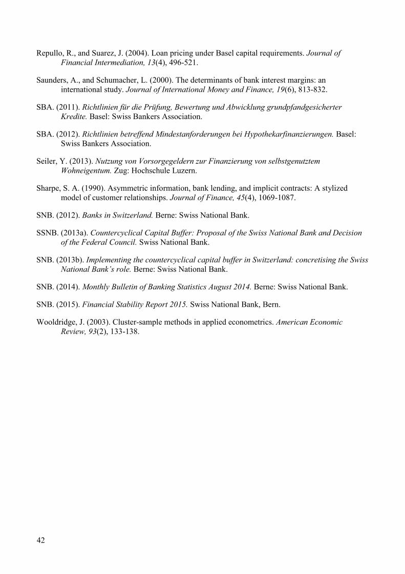
42
Repullo, R., and Suarez, J. (2004). Loan pricing under Basel capital requirements. Journal of
Financial Intermediation, 13(4), 496-521.
Saunders, A., and Schumacher, L. (2000). The determinants of bank interest margins: an
international study. Journal of International Money and Finance, 19(6), 813-832.
SBA. (2011). Richtlinien für die Prüfung, Bewertung und Abwicklung grundpfandgesicherter
Kredite. Basel: Swiss Bankers Association.
SBA. (2012). Richtlinien betreffend Mindestanforderungen bei Hypothekarfinanzierungen. Basel:
Swiss Bankers Association.
Seiler, Y. (2013). Nutzung von Vorsorgegeldern zur Finanzierung von selbstgenutztem
Wohneigentum. Zug: Hochschule Luzern.
Sharpe, S. A. (1990). Asymmetric information, bank lending, and implicit contracts: A stylized
model of customer relationships. Journal of Finance, 45(4), 1069-1087.
SNB. (2012). Banks in Switzerland. Berne: Swiss National Bank.
SSNB. (2013a). Countercyclical Capital Buffer: Proposal of the Swiss National Bank and Decision
of the Federal Council. Swiss National Bank.
SNB. (2013b). Implementing the countercyclical capital buffer in Switzerland: concretising the Swiss
National Bank’s role. Berne: Swiss National Bank.
SNB. (2014). Monthly Bulletin of Banking Statistics August 2014. Berne: Swiss National Bank.
SNB. (2015). Financial Stability Report 2015. Swiss National Bank, Bern.
Wooldridge, J. (2003). Cluster-sample methods in applied econometrics. American Economic
Review, 93(2), 133-138.
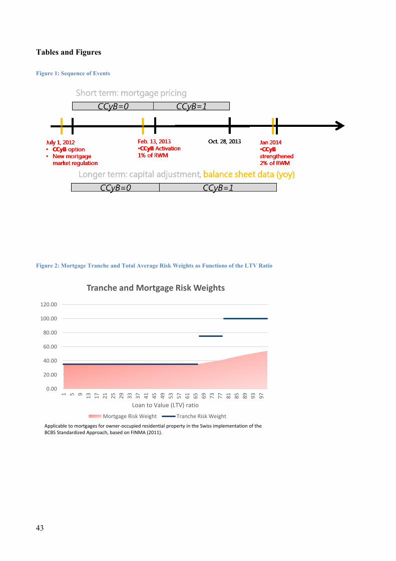
43
Tables and Figures
Figure 1: Sequence of Events
Figure 2: Mortgage Tranche and Total Average Risk Weights as Functions of the LTV Ratio
0.00
20.00
40.00
60.00
80.00
100.00
120.00
1 5 9
13
17
21
25
29
33
37
41
45
49
53
57
61
65
69
73
77
81
85
89
93
97
Loan to Value (LTV) ratio
Tranche and Mortgage Risk Weights
Mortgage Risk Weight Tranche Risk Weight
Applicable to mortgages for owner-occupied residential property in the Swiss implementation of the BCBS Standardized Approach, based on FINMA (2011).
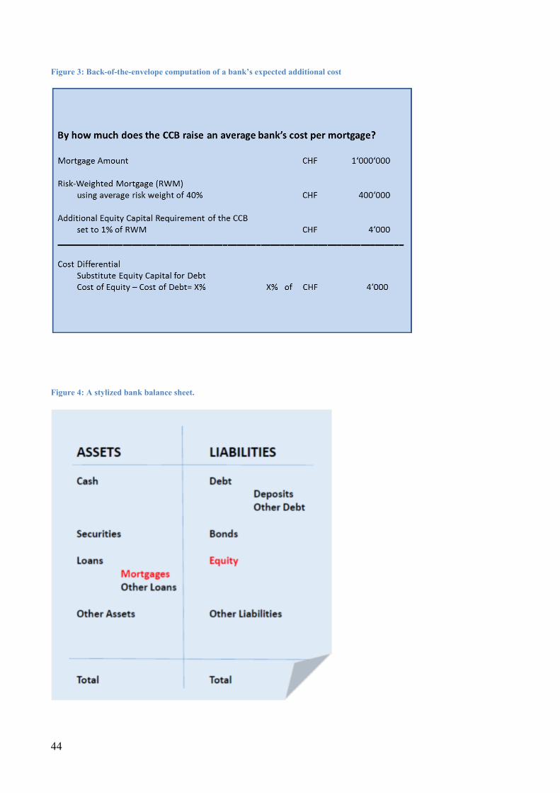
44
Figure 3: Back-of-the-envelope computation of a bank’s expected additional cost
Figure 4: A stylized bank balance sheet.
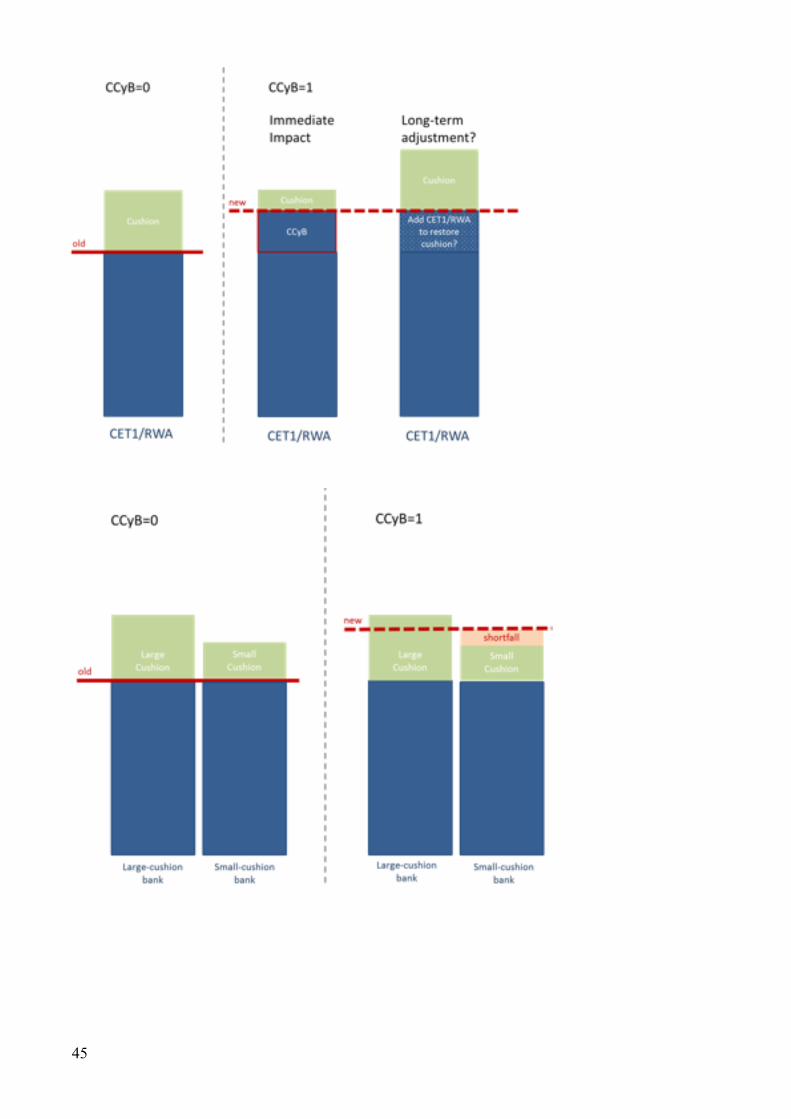
45
Figure 5: Immediate impact of the CCyB and longer-term adjustment
The CCyB immediately reduces the capital cushion that banks set aside. Over time, they might restore the
capital cushion to the pre-CCyB level, or prefer to operate with a lower cushion.
Figure 6: Differential immediate impact: How big was the cushion?
Low cushion banks might see a capital shortage and will need to raise capital urgently.
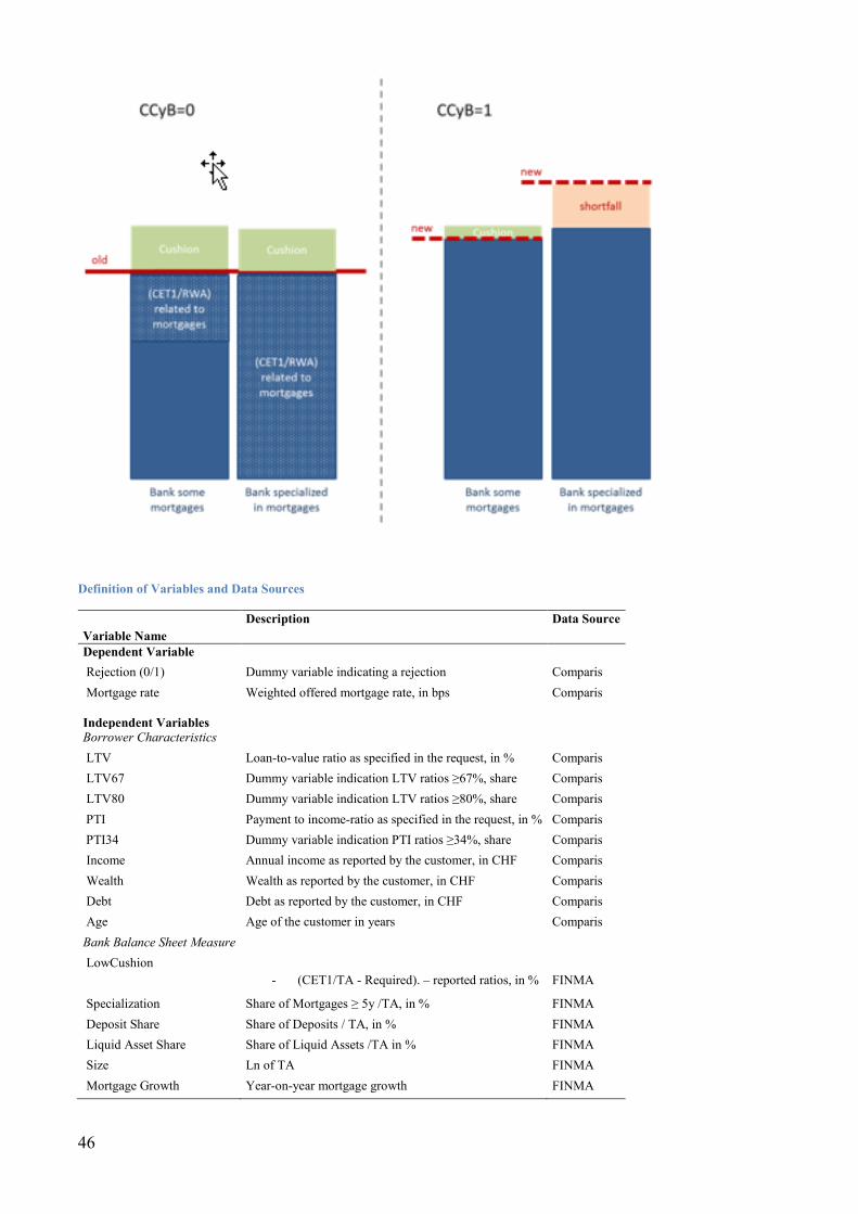
46
Figure 7: Differential immediate impact: banks with a specialization in the mortgage business
CCyB imposes a higher burden on specialized banks.
Definition of Variables and Data Sources
Variable Name
Description Data Source
Dependent Variable
Rejection (0/1) Dummy variable indicating a rejection Comparis
Mortgage rate
Independent Variables
Weighted offered mortgage rate, in bps Comparis
Borrower Characteristics
LTV Loan-to-value ratio as specified in the request, in % Comparis
LTV67 Dummy variable indication LTV ratios ≥67%, share Comparis
LTV80 Dummy variable indication LTV ratios ≥80%, share Comparis
PTI Payment to income-ratio as specified in the request, in % Comparis
PTI34 Dummy variable indication PTI ratios ≥34%, share Comparis
Income Annual income as reported by the customer, in CHF Comparis
Wealth Wealth as reported by the customer, in CHF Comparis
Debt Debt as reported by the customer, in CHF Comparis
Age Age of the customer in years Comparis
Bank Balance Sheet Measure
LowCushion
- (CET1/TA - Required). – reported ratios, in % FINMA
Specialization Share of Mortgages ≥ 5y /TA, in % FINMA
Deposit Share Share of Deposits / TA, in % FINMA
Liquid Asset Share Share of Liquid Assets /TA in % FINMA
Size Ln of TA FINMA
Mortgage Growth Year-on-year mortgage growth FINMA
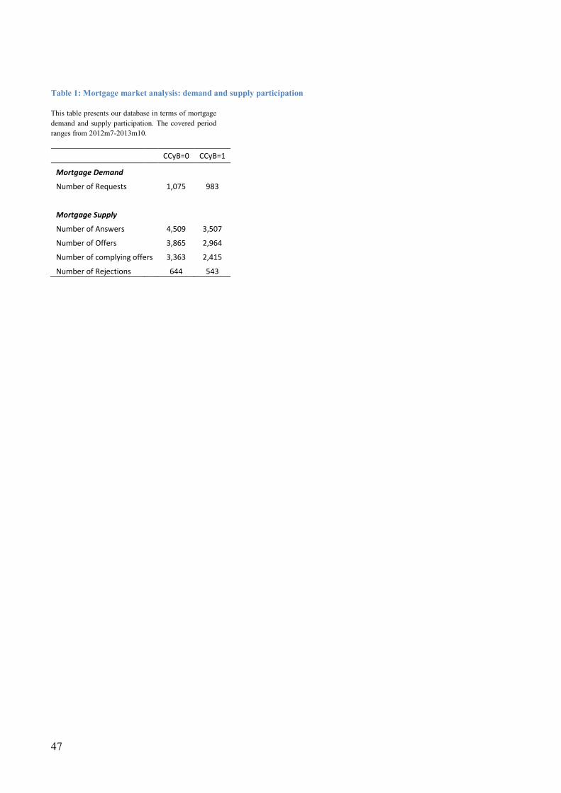
47
Table 1: Mortgage market analysis: demand and supply participation
This table presents our database in terms of mortgage
demand and supply participation. The covered period
ranges from 2012m7-2013m10.
CCyB=0 CCyB=1
Mortgage Demand
Number of Requests 1,075 983
Mortgage Supply
Number of Answers 4,509 3,507
Number of Offers 3,865 2,964
Number of complying offers 3,363 2,415
Number of Rejections 644 543
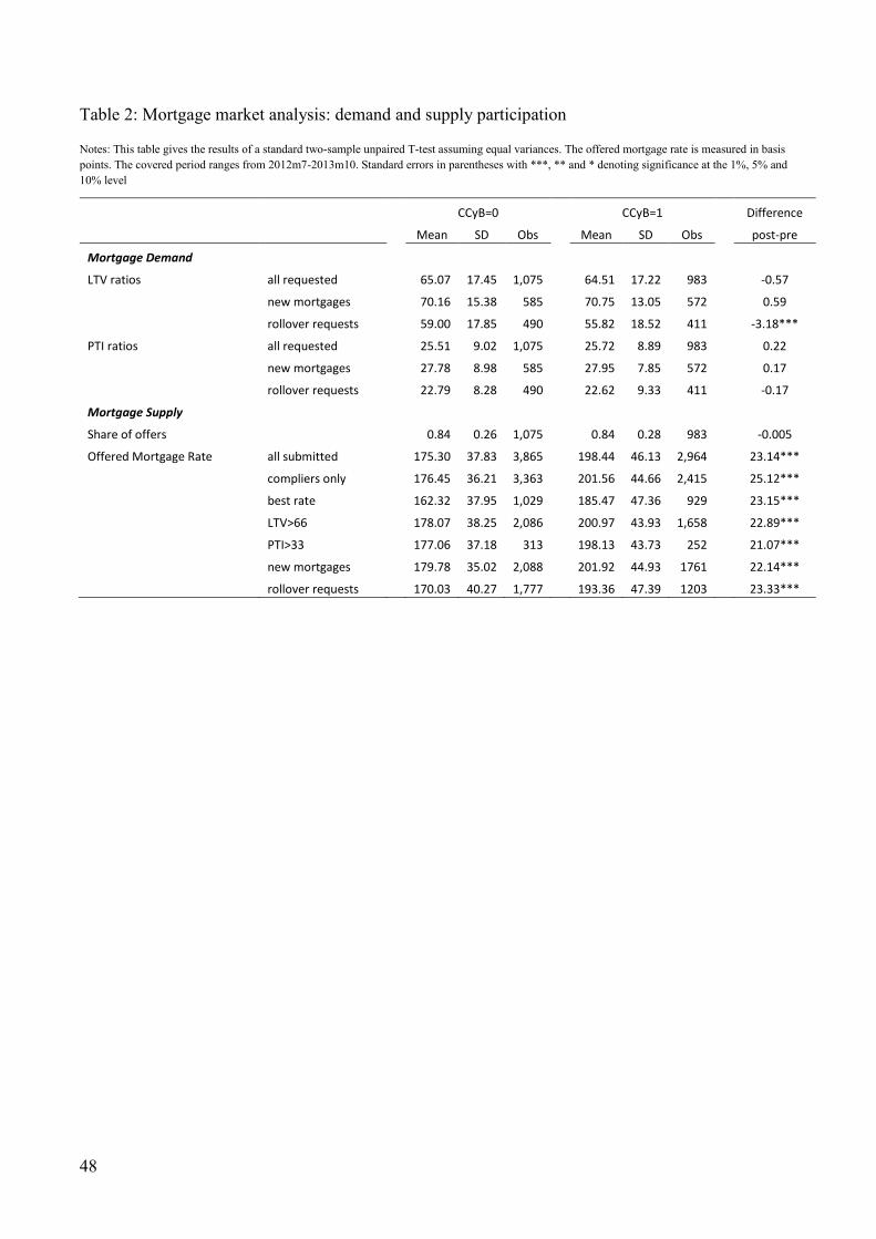
48
Table 2: Mortgage market analysis: demand and supply participation
Notes: This table gives the results of a standard two-sample unpaired T-test assuming equal variances. The offered mortgage rate is measured in basis
points. The covered period ranges from 2012m7-2013m10. Standard errors in parentheses with ***, ** and * denoting significance at the 1%, 5% and
10% level
CCyB=0 CCyB=1 Difference
Mean SD Obs Mean SD Obs post-pre
Mortgage Demand
LTV ratios all requested 65.07 17.45 1,075 64.51 17.22 983 -0.57
new mortgages 70.16 15.38 585 70.75 13.05 572 0.59
rollover requests 59.00 17.85 490 55.82 18.52 411 -3.18***
PTI ratios all requested 25.51 9.02 1,075 25.72 8.89 983 0.22
new mortgages 27.78 8.98 585 27.95 7.85 572 0.17
rollover requests 22.79 8.28 490 22.62 9.33 411 -0.17
Mortgage Supply
Share of offers 0.84 0.26 1,075 0.84 0.28 983 -0.005
Offered Mortgage Rate all submitted 175.30 37.83 3,865 198.44 46.13 2,964 23.14***
compliers only 176.45 36.21 3,363 201.56 44.66 2,415 25.12***
best rate 162.32 37.95 1,029 185.47 47.36 929 23.15***
LTV˃66 178.07 38.25 2,086 200.97 43.93 1,658 22.89***
PTI˃33 177.06 37.18 313 198.13 43.73 252 21.07***
new mortgages 179.78 35.02 2,088 201.92 44.93 1761 22.14***
rollover requests 170.03 40.27 1,777 193.36 47.39 1203 23.33***
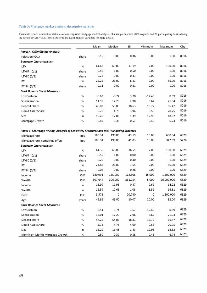
49
Table 3: Mortgage market analysis, descriptive statistics
This table reports descriptive statistics of our empirical mortgage market analysis. Our sample features 2058 requests and 21 participating banks during
the period 2012m7 to 2013m10. Refer to the Definition of Variables for more details.
Mean Median SD Minimum Maximum Obs
Panel A: Offer/Reject Analysis
rejection (0/1) share 0.15 0.00 0.36 0.00 1.00 8016
Borrower Characteristics
LTV % 64.62 69.00 17.19 7.00 100.00 8016
LTV67 (0/1) share 0.56 1.00 0.50 0.00 1.00 8016
LTV80 (0/1) share 0.22 0.00 0.41 0.00 1.00 8016
PTI % 25.25 26.00 8.43 2.00 86.00 8016
PTI34 (0/1) share 0.11 0.00 0.31 0.00 1.00 8016
Bank Balance Sheet Measures
LowCushion % -5.63 -5.74 3.70 -12.45 0.59 8016
Specialization % 11.95 12.29 2.98 6.62 21.94 8016
Deposit Share % 48.03 55.05 18.63 16.72 66.47 8016
Liquid Asset Share % 5.76 4.78 3.94 0.56 20.75 8016
Size ln 16.20 17.06 1.39 12.96 18.82 8016
Mortgage Growth % 0.49 0.38 0.57 -0.48 6.74 8016
Panel B: Mortgage Pricing, Analysis of Sensitivity Measures and Risk-Weighting Schemes
Mortgage rate bps 185.34 190.00 43.19 10.00 690.94 6829
Mortgage rate, complying offers bps 186.94 190.00 41.83 10.00 342.69 5778
Borrower Characteristics
LTV % 64.36 68.00 16.51 7.00 100.00 6829
LTV67 (0/1) share 0.55 1.00 0.00 0.00 1.00 6829
LTV80 (0/1) share 0.20 0.00 0.40 0.00 1.00 6829
PTI % 24.88 26.00 7.64 2.00 86.00 6829
PTI34 (0/1) share 0.08 0.00 0.28 0.00 1.00 6829
Income CHF 180,991 155,000 112,806 15,000 1,500,000 6829
Wealth CHF 507,044 306,000 861,054 5,000 20,000,000 6829
Income ln 11.99 11.95 0.47 9.62 14.22 6829
Wealth ln 12.59 12.63 1.08 8.52 16.81 6829
Debt CHF 3,573 0 20,740 0 1,300,000 6829
Age years 45.86 45.00 10.07 20.00 82.00 6829
Bank Balance Sheet Measures
LowCushion % -5.51 -5.74 3.67 -12.45 0.59 6829
Specialization % 12.01 12.29 2.96 6.62 21.94 6829
Deposit Share % 47.25 54.06 18.83 16.72 66.47 6829
Liquid Asset Share % 5.73 4.78 4.09 0.56 20.75 6829
Size ln 16.20 16.48 1.43 12.96 18.82 6829
Month-on-Month Mortgage Growth % 0.50 0.39 0.58 -0.48 6.74 6829
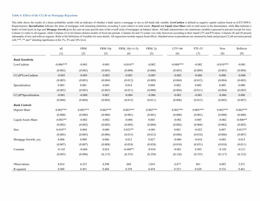
Table 4: Effect of the CCyB on Mortgage Rejections
This table shows the results of a linear probability model with an indicator of whether a bank rejects a mortgage or not as left-hand side variable. LowCushion is defined as negative capital cushion based on (CET1/RWA-
Requirements). Specialization indicates the share of mortgages with remaining maturities exceeding 5 years relative to total assets. Deposit and Liquid Asset Share refer to total assets in the denominator, while Size indicates a
bank's of total assets in logs and Mortgage Growth gives the year-on-year growth rates of the overall stock of mortgages on balance sheets. All bank characteristics are continuous variables expressed in percent (except for size).
Column (1) refers to all requests, while Columns (2) to (6) feature distinct models of fixed rate periods. Columns (6) and (7) isolate very risky borrowers according to their stated LTV and PTI ratios, Columns (8) and (9) present
subsamples of new and rollover requests. Refer to the Definition of Variables for more details. All regressions include request fixed effects. Standard errors in parentheses are clustered by bank and pre/post CCyB activation period
with ***, ** and * denoting significance at the 1%, 5% and 10% level.
all FRM FRM 10y FRM, 10y˃x˃5y FRM, 5y LTV˃66 PTI˃33 New Rollover
(1) (2) (3) (4) (5) (6) (7) (8) (9)
Bank Sensitivity
LowCushion -0.006*** -0.003 -0.001 -0.016** -0.002 -0.008*** -0.002 -0.010*** -0.001
(0.002) (0.002) (0.003) (0.008) (0.006) (0.003) (0.009) (0.003) (0.004)
CCyB*LowCushion -0.003 -0.003 -0.003 -0.001 -0.005 -0.002 -0.006 0.000 -0.006
(0.003) (0.003) (0.004) (0.012) (0.009) (0.004) (0.012) (0.004) (0.005)
Specialization 0.003 0.001 -0.001 0.014 0.004 0.002 0.002 0.005 0.000
(0.003) (0.003) (0.003) (0.011) (0.008) (0.004) (0.011) (0.004) (0.005)
CCyB*Specialization -0.001 -0.000 0.003 -0.004 -0.006 -0.001 -0.001 -0.006 0.006
(0.004) (0.004) (0.005) (0.015) (0.011) (0.006) (0.015) (0.005) (0.007)
Bank Controls
Deposit Share 0.002*** 0.002*** 0.002*** 0.003*** 0.002*** 0.002*** 0.003*** 0.002*** 0.002***
(0.000) (0.000) (0.000) (0.001) (0.001) (0.000) (0.001) (0.000) (0.000)
Liquid Assets Share -0.003** -0.002 -0.002 -0.006 0.003 -0.002 0.005 -0.002 -0.006**
(0.002) (0.002) (0.002) (0.005) (0.004) (0.002) (0.006) (0.002) (0.002)
Size 0.010** 0.004 0.000 0.032** -0.001 0.001 -0.022 0.007 0.015**
(0.005) (0.005) (0.006) (0.015) (0.012) (0.006) (0.016) (0.006) (0.007)
Mortgage Growth, yoy 0.006 0.009 0.006 0.012 0.027 -0.006 -0.018 -0.001 0.015
(0.007) (0.007) (0.008) (0.024) (0.024) (0.010) (0.031) (0.010) (0.011)
Constant -0.145 -0.060 0.024 -0.680** -0.010 -0.001 0.503 -0.105 -0.211
(0.093) (0.098) (0.115) (0.333) (0.250) (0.126) (0.335) (0.117) (0.152)
Observations 8,016 6,523 4,598 668 1,016 4,477 861 4,485 3,531
R-squared 0.488 0.491 0.484 0.558 0.454 0.523 0.620 0.516 0.461
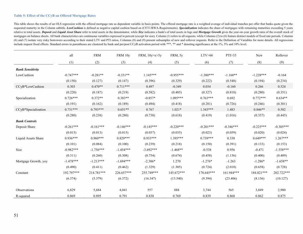
51
Table 5: Effect of the CCyB on Offered Mortgage Rates
This table shows the results of an OLS regression with the offered mortgage rate as dependent variable in basis points. The offered mortgage rate is a weighted average of individual tranches per offer that banks quote given the
requested maturity in the Column subtitle. LowCushion is defined as negative capital cushion based on (CET1/RWA-Requirements). Specialization indicates the share of mortgages with remaining maturities exceeding 5 years
relative to total assets. Deposit and Liquid Asset Share refer to total assets in the denominator, while Size indicates a bank's of total assets in logs and Mortgage Growth gives the year-on-year growth rates of the overall stock of
mortgages on balance sheets. All bank characteristics are continuous variables expressed in percent (except for size). Column (1) refers to all requests, while Columns (2) to (6) feature distinct models of fixed rate periods. Columns
(6) and (7) isolate very risky borrowers according to their stated LTV and PTI ratios, Columns (8) and (9) present subsamples of new and rollover requests. Refer to the Definition of Variables for more details. All regressions
include request fixed effects. Standard errors in parentheses are clustered by bank and pre/post CCyB activation period with ***, ** and * denoting significance at the 1%, 5% and 10% level.
all FRM FRM 10y FRM, 10y˃x˃5y FRM, 5y LTV˃66 PTI˃33 New Rollover
(1) (2) (3) (4) (5) (6) (7) (8) (9)
Bank Sensitivity
LowCushion -0.747*** -0.281** -0.331** 1.145*** -0.955*** -1.380*** -1.160** -1.228*** -0.164
(0.150) (0.127) (0.147) (0.396) (0.329) (0.222) (0.548) (0.194) (0.234)
CCyB*LowCushion 0.303 0.470** 0.711*** 0.497 -0.349 0.034 -0.160 0.266 0.524
(0.220) (0.187) (0.219) (0.582) (0.485) (0.327) (0.818) (0.280) (0.351)
Specialization 0.726*** 0.372** 0.383** -0.857* 1.095*** 0.763*** 0.692 0.772*** 0.634**
(0.191) (0.162) (0.189) (0.494) (0.418) (0.281) (0.726) (0.246) (0.301)
CCyB*Specialization 0.731*** 0.793*** 0.651** 0.767 1.021* 1.343*** 1.483 0.846** 0.502
(0.280) (0.238) (0.280) (0.738) (0.618) (0.419) (1.016) (0.357) (0.445)
Bank Controls
Deposit Share -0.261*** -0.161*** -0.146*** -0.145*** -0.220*** -0.201*** -0.346*** -0.225*** -0.305***
(0.015) (0.013) (0.015) (0.037) (0.035) (0.023) (0.059) (0.020) (0.024)
Liquid Assets Share 0.936*** 0.960*** 0.829*** 0.933*** 1.395*** 0.739*** 0.330 0.649*** 1.267***
(0.101) (0.084) (0.100) (0.239) (0.218) (0.150) (0.391) (0.133) (0.153)
Size -0.982*** -1.756*** -1.454*** -3.692*** -1.468** -0.538 0.956 -0.471 -1.558***
(0.311) (0.260) (0.308) (0.754) (0.674) (0.458) (1.136) (0.400) (0.489)
Mortgage Growth, yoy -1.478*** -1.213*** -1.694*** -2.386* 1.270 -1.276* -1.263 -1.286* -1.658**
(0.490) (0.411) (0.462) (1.329) (1.305) (0.724) (2.018) (0.658) (0.728)
Constant 192.797*** 214.781*** 226.657*** 255.749*** 145.672*** 178.645*** 161.944*** 184.821*** 202.722***
(6.374) (5.379) (6.372) (16.347) (13.540) (9.394) (23.406) (8.136) (10.127)
Observations 6,829 5,684 4,041 557 888 3,744 565 3,849 2,980
R-squared 0.869 0.895 0.791 0.838 0.769 0.839 0.868 0.862 0.875
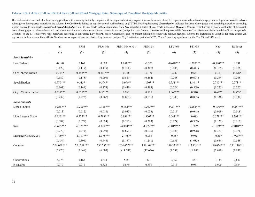
52
Table 6: Effect of the CCyB on Effect of the CCyB on Offered Mortgage Rates: Subsample of Compliant Mortgage Maturities
This table isolates our results for those mortgage offers with a maturity that fully complies with the requested maturity. Again, it shows the results of an OLS regression with the offered mortgage rate as dependent variable in basis
points, given the requested maturity in the column. LowCushion is defined as negative capital cushion based on (CET1/RWA-Requirements). Specialization indicates the share of mortgages with remaining maturities exceeding
5 years relative to total assets. Deposit and Liquid Asset Share refer to total assets in the denominator, while Size indicates a bank's of total assets in logs and Mortgage Growth gives the year-on-year growth rates of the overall
stock of mortgages on balance sheets. All bank characteristics are continuous variables expressed in percent (except for size). Column (1) refers to all requests, while Columns (2) to (6) feature distinct models of fixed rate periods.
Columns (6) and (7) isolate very risky borrowers according to their stated LTV and PTI ratios, Columns (8) and (9) present subsamples of new and rollover requests. Refer to the Definition of Variables for more details. All
regressions include request fixed effects. Standard errors in parentheses are clustered by bank and pre/post CCyB activation period with ***, ** and * denoting significance at the 1%, 5% and 10% level.
all FRM FRM 10y FRM, 10y˃x˃5y FRM, 5y LTV˃66 PTI˃33 New Rollover
(1) (2) (3) (4) (5) (6) (7) (8) (9)
Bank Sensitivity
LowCushion -0.190 0.167 0.093 1.651*** -0.503 -0.678*** -1.297*** -0.590*** 0.191
(0.129) (0.119) (0.139) (0.358) (0.307) (0.185) (0.441) (0.185) (0.176)
CCyB*LowCushion 0.324* 0.542*** 0.801*** 0.318 -0.180 0.049 0.641 0.311 0.498*
(0.189) (0.175) (0.206) (0.521) (0.454) (0.268) (0.671) (0.264) (0.265)
Specialization 0.770*** 0.383** 0.394** -0.990** 1.190*** 0.951*** 1.444** 0.780*** 0.773***
(0.161) (0.149) (0.174) (0.440) (0.383) (0.224) (0.569) (0.225) (0.225)
CCyB*Specialization 0.657*** 0.670*** 0.551** 0.983 0.727 1.065*** 0.340 0.627* 0.563*
(0.239) (0.222) (0.262) (0.657) (0.576) (0.340) (0.805) (0.336) (0.334)
Bank Controls
Deposit Share -0.238*** -0.200*** -0.186*** -0.162*** -0.267*** -0.207*** -0.282*** -0.196*** -0.287***
(0.013) (0.012) (0.014) (0.033) (0.033) (0.019) (0.048) (0.019) (0.018)
Liquid Assets Share 0.956*** 0.925*** 0.799*** 0.899*** 1.300*** 0.641*** 0.083 0.571*** 1.391***
(0.087) (0.079) (0.094) (0.217) (0.203) (0.124) (0.309) (0.127) (0.116)
Size -1.605*** -2.129*** -1.814*** -4.080*** -1.722*** -1.019*** 1.682* -1.109*** -2.010***
(0.270) (0.247) (0.294) (0.691) (0.635) (0.383) (0.928) (0.383) (0.371)
Mortgage Growth, yoy -1.190*** -1.117*** -1.378*** -2.776** 0.098 -0.387 0.985 -0.307 -1.975***
(0.434) (0.394) (0.446) (1.187) (1.241) (0.631) (1.683) (0.664) (0.548)
Constant 206.068*** 224.368*** 236.235*** 264.657*** 154.468*** 190.335*** 147.951*** 199.634*** 211.119***
(5.470) (5.048) (6.007) (14.787) (12.676) (7.732) (19.096) (7.680) (7.632)
Observations 5,778 5,165 3,644 516 821 2,962 457 3,139 2,639
R-squared 0.917 0.917 0.824 0.879 0.799 0.913 0.931 0.900 0.934
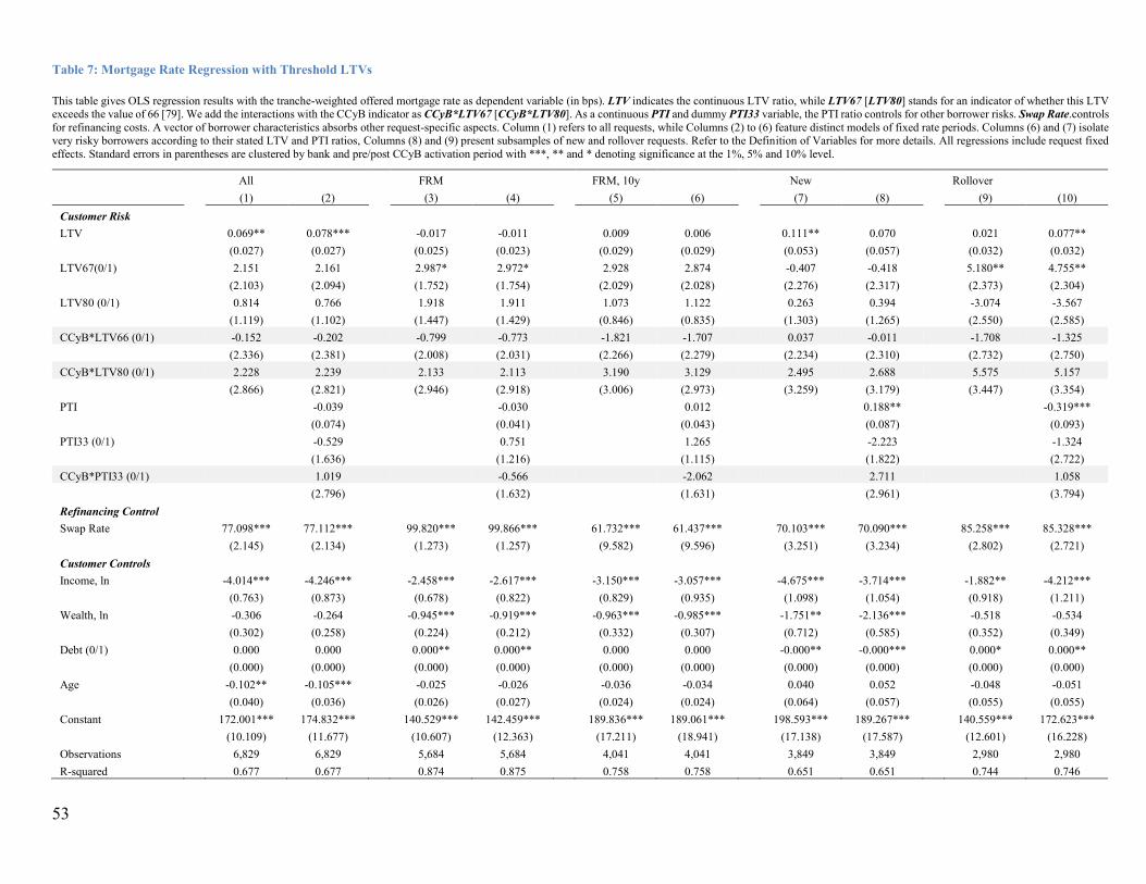
53
Table 7: Mortgage Rate Regression with Threshold LTVs
This table gives OLS regression results with the tranche-weighted offered mortgage rate as dependent variable (in bps). LTV indicates the continuous LTV ratio, while LTV67 [LTV80] stands for an indicator of whether this LTV exceeds the value of 66 [79]. We add the interactions with the CCyB indicator as CCyB*LTV67 [CCyB*LTV80]. As a continuous PTI and dummy PTI33 variable, the PTI ratio controls for other borrower risks. Swap Rate.controls
for refinancing costs. A vector of borrower characteristics absorbs other request-specific aspects. Column (1) refers to all requests, while Columns (2) to (6) feature distinct models of fixed rate periods. Columns (6) and (7) isolate very risky borrowers according to their stated LTV and PTI ratios, Columns (8) and (9) present subsamples of new and rollover requests. Refer to the Definition of Variables for more details. All regressions include request fixed
effects. Standard errors in parentheses are clustered by bank and pre/post CCyB activation period with ***, ** and * denoting significance at the 1%, 5% and 10% level.
All FRM FRM, 10y New Rollover
(1) (2) (3) (4) (5) (6) (7) (8) (9) (10)
Customer Risk LTV 0.069** 0.078*** -0.017 -0.011 0.009 0.006 0.111** 0.070 0.021 0.077**
(0.027) (0.027) (0.025) (0.023) (0.029) (0.029) (0.053) (0.057) (0.032) (0.032)
LTV67(0/1) 2.151 2.161 2.987* 2.972* 2.928 2.874 -0.407 -0.418 5.180** 4.755**
(2.103) (2.094) (1.752) (1.754) (2.029) (2.028) (2.276) (2.317) (2.373) (2.304)
LTV80 (0/1) 0.814 0.766 1.918 1.911 1.073 1.122 0.263 0.394 -3.074 -3.567
(1.119) (1.102) (1.447) (1.429) (0.846) (0.835) (1.303) (1.265) (2.550) (2.585)
CCyB*LTV66 (0/1) -0.152 -0.202 -0.799 -0.773 -1.821 -1.707 0.037 -0.011 -1.708 -1.325
(2.336) (2.381) (2.008) (2.031) (2.266) (2.279) (2.234) (2.310) (2.732) (2.750)
CCyB*LTV80 (0/1) 2.228 2.239 2.133 2.113 3.190 3.129 2.495 2.688 5.575 5.157
(2.866) (2.821) (2.946) (2.918) (3.006) (2.973) (3.259) (3.179) (3.447) (3.354)
PTI -0.039 -0.030 0.012 0.188** -0.319***
(0.074) (0.041) (0.043) (0.087) (0.093)
PTI33 (0/1) -0.529 0.751 1.265 -2.223 -1.324
(1.636) (1.216) (1.115) (1.822) (2.722)
CCyB*PTI33 (0/1) 1.019 -0.566 -2.062 2.711 1.058
(2.796) (1.632) (1.631) (2.961) (3.794)
Refinancing Control Swap Rate 77.098*** 77.112*** 99.820*** 99.866*** 61.732*** 61.437*** 70.103*** 70.090*** 85.258*** 85.328***
(2.145) (2.134) (1.273) (1.257) (9.582) (9.596) (3.251) (3.234) (2.802) (2.721)
Customer Controls Income, ln -4.014*** -4.246*** -2.458*** -2.617*** -3.150*** -3.057*** -4.675*** -3.714*** -1.882** -4.212***
(0.763) (0.873) (0.678) (0.822) (0.829) (0.935) (1.098) (1.054) (0.918) (1.211)
Wealth, ln -0.306 -0.264 -0.945*** -0.919*** -0.963*** -0.985*** -1.751** -2.136*** -0.518 -0.534
(0.302) (0.258) (0.224) (0.212) (0.332) (0.307) (0.712) (0.585) (0.352) (0.349)
Debt (0/1) 0.000 0.000 0.000** 0.000** 0.000 0.000 -0.000** -0.000*** 0.000* 0.000**
(0.000) (0.000) (0.000) (0.000) (0.000) (0.000) (0.000) (0.000) (0.000) (0.000)
Age -0.102** -0.105*** -0.025 -0.026 -0.036 -0.034 0.040 0.052 -0.048 -0.051
(0.040) (0.036) (0.026) (0.027) (0.024) (0.024) (0.064) (0.057) (0.055) (0.055)
Constant 172.001*** 174.832*** 140.529*** 142.459*** 189.836*** 189.061*** 198.593*** 189.267*** 140.559*** 172.623***
(10.109) (11.677) (10.607) (12.363) (17.211) (18.941) (17.138) (17.587) (12.601) (16.228)
Observations 6,829 6,829 5,684 5,684 4,041 4,041 3,849 3,849 2,980 2,980
R-squared 0.677 0.677 0.874 0.875 0.758 0.758 0.651 0.651 0.744 0.746
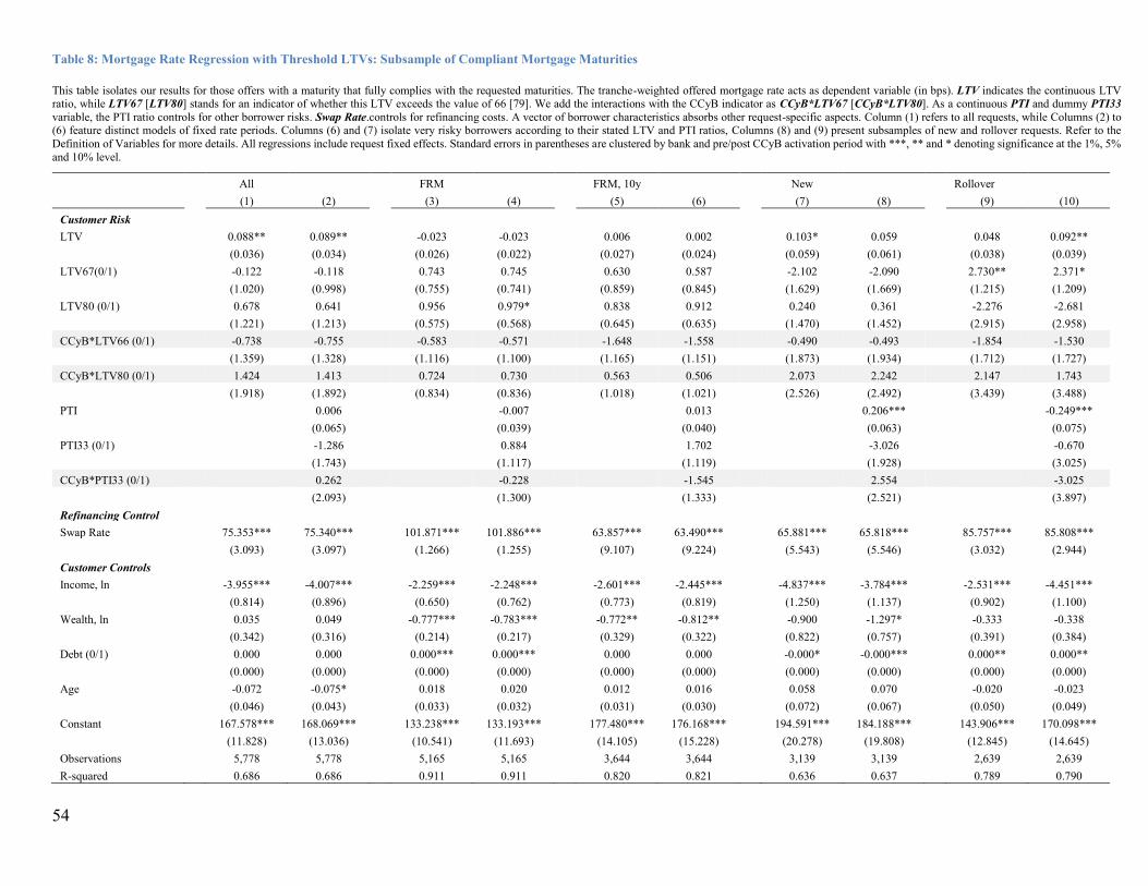
54
Table 8: Mortgage Rate Regression with Threshold LTVs: Subsample of Compliant Mortgage Maturities
This table isolates our results for those offers with a maturity that fully complies with the requested maturities. The tranche-weighted offered mortgage rate acts as dependent variable (in bps). LTV indicates the continuous LTV ratio, while LTV67 [LTV80] stands for an indicator of whether this LTV exceeds the value of 66 [79]. We add the interactions with the CCyB indicator as CCyB*LTV67 [CCyB*LTV80]. As a continuous PTI and dummy PTI33
variable, the PTI ratio controls for other borrower risks. Swap Rate.controls for refinancing costs. A vector of borrower characteristics absorbs other request-specific aspects. Column (1) refers to all requests, while Columns (2) to (6) feature distinct models of fixed rate periods. Columns (6) and (7) isolate very risky borrowers according to their stated LTV and PTI ratios, Columns (8) and (9) present subsamples of new and rollover requests. Refer to the
Definition of Variables for more details. All regressions include request fixed effects. Standard errors in parentheses are clustered by bank and pre/post CCyB activation period with ***, ** and * denoting significance at the 1%, 5%
and 10% level.
All FRM FRM, 10y New Rollover
(1) (2) (3) (4) (5) (6) (7) (8) (9) (10)
Customer Risk LTV 0.088** 0.089** -0.023 -0.023 0.006 0.002 0.103* 0.059 0.048 0.092**
(0.036) (0.034) (0.026) (0.022) (0.027) (0.024) (0.059) (0.061) (0.038) (0.039)
LTV67(0/1) -0.122 -0.118 0.743 0.745 0.630 0.587 -2.102 -2.090 2.730** 2.371*
(1.020) (0.998) (0.755) (0.741) (0.859) (0.845) (1.629) (1.669) (1.215) (1.209)
LTV80 (0/1) 0.678 0.641 0.956 0.979* 0.838 0.912 0.240 0.361 -2.276 -2.681
(1.221) (1.213) (0.575) (0.568) (0.645) (0.635) (1.470) (1.452) (2.915) (2.958)
CCyB*LTV66 (0/1) -0.738 -0.755 -0.583 -0.571 -1.648 -1.558 -0.490 -0.493 -1.854 -1.530
(1.359) (1.328) (1.116) (1.100) (1.165) (1.151) (1.873) (1.934) (1.712) (1.727)
CCyB*LTV80 (0/1) 1.424 1.413 0.724 0.730 0.563 0.506 2.073 2.242 2.147 1.743
(1.918) (1.892) (0.834) (0.836) (1.018) (1.021) (2.526) (2.492) (3.439) (3.488)
PTI 0.006 -0.007 0.013 0.206*** -0.249***
(0.065) (0.039) (0.040) (0.063) (0.075)
PTI33 (0/1) -1.286 0.884 1.702 -3.026 -0.670
(1.743) (1.117) (1.119) (1.928) (3.025)
CCyB*PTI33 (0/1) 0.262 -0.228 -1.545 2.554 -3.025
(2.093) (1.300) (1.333) (2.521) (3.897)
Refinancing Control Swap Rate 75.353*** 75.340*** 101.871*** 101.886*** 63.857*** 63.490*** 65.881*** 65.818*** 85.757*** 85.808***
(3.093) (3.097) (1.266) (1.255) (9.107) (9.224) (5.543) (5.546) (3.032) (2.944)
Customer Controls Income, ln -3.955*** -4.007*** -2.259*** -2.248*** -2.601*** -2.445*** -4.837*** -3.784*** -2.531*** -4.451***
(0.814) (0.896) (0.650) (0.762) (0.773) (0.819) (1.250) (1.137) (0.902) (1.100)
Wealth, ln 0.035 0.049 -0.777*** -0.783*** -0.772** -0.812** -0.900 -1.297* -0.333 -0.338
(0.342) (0.316) (0.214) (0.217) (0.329) (0.322) (0.822) (0.757) (0.391) (0.384)
Debt (0/1) 0.000 0.000 0.000*** 0.000*** 0.000 0.000 -0.000* -0.000*** 0.000** 0.000**
(0.000) (0.000) (0.000) (0.000) (0.000) (0.000) (0.000) (0.000) (0.000) (0.000)
Age -0.072 -0.075* 0.018 0.020 0.012 0.016 0.058 0.070 -0.020 -0.023
(0.046) (0.043) (0.033) (0.032) (0.031) (0.030) (0.072) (0.067) (0.050) (0.049)
Constant 167.578*** 168.069*** 133.238*** 133.193*** 177.480*** 176.168*** 194.591*** 184.188*** 143.906*** 170.098***
(11.828) (13.036) (10.541) (11.693) (14.105) (15.228) (20.278) (19.808) (12.845) (14.645)
Observations 5,778 5,778 5,165 5,165 3,644 3,644 3,139 3,139 2,639 2,639
R-squared 0.686 0.686 0.911 0.911 0.820 0.821 0.636 0.637 0.789 0.790
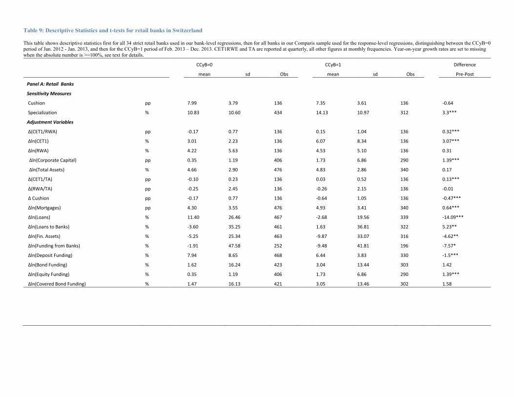
Table 9: Descriptive Statistics and t-tests for retail banks in Switzerland
This table shows descriptive statistics first for all 34 strict retail banks used in our bank-level regressions, then for all banks in our Comparis sample used for the response-level regressions, distinguishing between the CCyB=0 period of Jan. 2012 - Jan. 2013, and then for the CCyB=1 period of Feb. 2013 – Dec. 2013. CET1RWE and TA are reported at quarterly, all other figures at monthly frequencies. Year-on-year growth rates are set to missing
when the absolute number is >=100%, see text for details.
CCyB=0 CCyB=1 Difference
mean sd Obs mean sd Obs Pre-Post
Panel A: Retail Banks
Sensitivity Measures
Cushion pp 7.99 3.79 136 7.35 3.61 136 -0.64
Specialization % 10.83 10.60 434 14.13 10.97 312 3.3***
Adjustment Variables
∆(CET1/RWA) pp -0.17 0.77 136 0.15 1.04 136 0.32***
∆ln(CET1) % 3.01 2.23 136 6.07 8.34 136 3.07***
∆ln(RWA) % 4.22 5.63 136 4.53 5.10 136 0.31
∆ln(Corporate Capital) pp 0.35 1.19 406 1.73 6.86 290 1.39***
∆ln(Total Assets) % 4.66 2.90 476 4.83 2.86 340 0.17
∆(CET1/TA) pp -0.10 0.23 136 0.03 0.52 136 0.13***
∆(RWA/TA) pp -0.25 2.45 136 -0.26 2.15 136 -0.01
∆ Cushion pp -0.17 0.77 136 -0.64 1.05 136 -0.47***
∆ln(Mortgages) pp 4.30 3.55 476 4.93 3.41 340 0.64***
∆ln(Loans) % 11.40 26.46 467 -2.68 19.56 339 -14.09***
∆ln(Loans to Banks) % -3.60 35.25 461 1.63 36.81 322 5.23**
∆ln(Fin. Assets) % -5.25 25.34 463 -9.87 33.07 316 -4.62**
∆ln(Funding from Banks) % -1.91 47.58 252 -9.48 41.81 196 -7.57*
∆ln(Deposit Funding) % 7.94 8.65 468 6.44 3.83 330 -1.5***
∆ln(Bond Funding) % 1.62 16.24 423 3.04 13.44 303 1.42
∆ln(Equity Funding) % 0.35 1.19 406 1.73 6.86 290 1.39***
∆ln(Covered Bond Funding) % 1.47 16.13 421 3.05 13.46 302 1.58
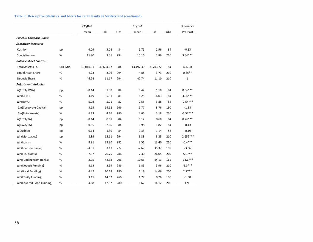
56
Table 9: Descriptive Statistics and t-tests for retail banks in Switzerland (continued)
CCyB=0 CCyB=1 Difference
mean sd Obs mean sd Obs Pre-Post
Panel B: Comparis Banks
Sensitivity Measures
Cushion pp 6.09 3.08 84 5.75 2.96 84 -0.33
Specialization % 11.80 3.01 294 15.16 2.86 210 3.36***
Balance Sheet Controls
Total Assets (TA) CHF Mio. 13,040.51 30,694.02 84 13,497.39 31703.22 84 456.88
Liquid Asset Share % 4.23 3.06 294 4.88 3.73 210 0.66**
Deposit Share % 46.94 11.17 294 47.74 11.10 210 1
Adjustment Variables
∆(CET1/RWA) pp -0.14 1.30 84 0.42 1.10 84 0.56***
∆ln(CET1) % 3.19 5.91 81 6.25 6.03 84 3.06***
∆ln(RWA) % 5.08 5.21 82 2.55 3.86 84 -2.54***
∆ln(Corporate Capital) pp 3.15 14.52 266 1.77 8.76 190 -1.38
∆ln(Total Assets) % 6.23 4.16 286 4.65 3.18 210 -1.57***
∆(CET1/TA) pp -0.14 0.61 84 0.12 0.60 84 0.26***
∆(RWA/TA) pp -0.55 2.66 84 -0.98 1.82 84 -0.43
∆ Cushion pp -0.14 1.30 84 -0.33 1.14 84 -0.19
∆ln(Mortgages) pp 8.89 15.11 294 6.38 3.35 210 -2.§52***
∆ln(Loans) % 8.91 23.80 281 2.51 13.40 210 -6.4***
∆ln(Loans to Banks) % -4.31 33.17 272 -7.67 35.37 199 -3.36
∆ln(Fin. Assets) % -7.37 20.75 286 -2.30 26.05 209 5.07**
∆ln(Funding from Banks) % 2.95 42.58 206 -10.65 44.13 165 -13.6***
∆ln(Deposit Funding) % 8.13 2.99 286 6.83 3.96 210 -1.3***
∆ln(Bond Funding) % 4.42 10.78 280 7.19 14.66 200 2.77**
∆ln(Equity Funding) % 3.15 14.52 266 1.77 8.76 190 -1.38
∆ln(Covered Bond Funding) % 4.68 12.92 280 6.67 14.12 200 1.99
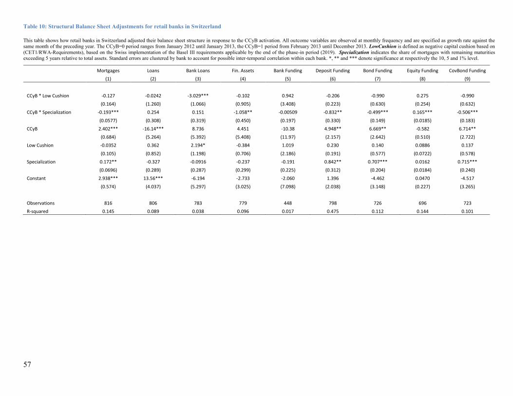
57
Table 10: Structural Balance Sheet Adjustments for retail banks in Switzerland
This table shows how retail banks in Switzerland adjusted their balance sheet structure in response to the CCyB activation. All outcome variables are observed at monthly frequency and are specified as growth rate against the same month of the preceding year. The CCyB=0 period ranges from January 2012 until January 2013, the CCyB=1 period from February 2013 until December 2013. LowCushion is defined as negative capital cushion based on
(CET1/RWA-Requirements), based on the Swiss implementation of the Basel III requirements applicable by the end of the phase-in period (2019). Specialization indicates the share of mortgages with remaining maturities exceeding 5 years relative to total assets. Standard errors are clustered by bank to account for possible inter-temporal correlation within each bank. *, ** and *** denote significance at respectively the 10, 5 and 1% level.
Mortgages Loans Bank Loans Fin. Assets Bank Funding Deposit Funding Bond Funding Equity Funding CovBond Funding
(1) (2) (3) (4) (5) (6) (7) (8) (9)
CCyB * Low Cushion -0.127 -0.0242 -3.029*** -0.102 0.942 -0.206 -0.990 0.275 -0.990
(0.164) (1.260) (1.066) (0.905) (3.408) (0.223) (0.630) (0.254) (0.632)
CCyB * Specialization -0.193*** 0.254 0.151 -1.058** -0.00509 -0.832** -0.499*** 0.165*** -0.506***
(0.0577) (0.308) (0.319) (0.450) (0.197) (0.330) (0.149) (0.0185) (0.183)
CCyB 2.402*** -16.14*** 8.736 4.451 -10.38 4.948** 6.669** -0.582 6.714**
(0.684) (5.264) (5.392) (5.408) (11.97) (2.157) (2.642) (0.510) (2.722)
Low Cushion -0.0352 0.362 2.194* -0.384 1.019 0.230 0.140 0.0886 0.137
(0.105) (0.852) (1.198) (0.706) (2.186) (0.191) (0.577) (0.0722) (0.578)
Specialization 0.172** -0.327 -0.0916 -0.237 -0.191 0.842** 0.707*** 0.0162 0.715***
(0.0696) (0.289) (0.287) (0.299) (0.225) (0.312) (0.204) (0.0184) (0.240)
Constant 2.938*** 13.56*** -6.194 -2.733 -2.060 1.396 -4.462 0.0470 -4.517
(0.574) (4.037) (5.297) (3.025) (7.098) (2.038) (3.148) (0.227) (3.265)
Observations 816 806 783 779 448 798 726 696 723
R-squared 0.145 0.089 0.038 0.096 0.017 0.475 0.112 0.144 0.101
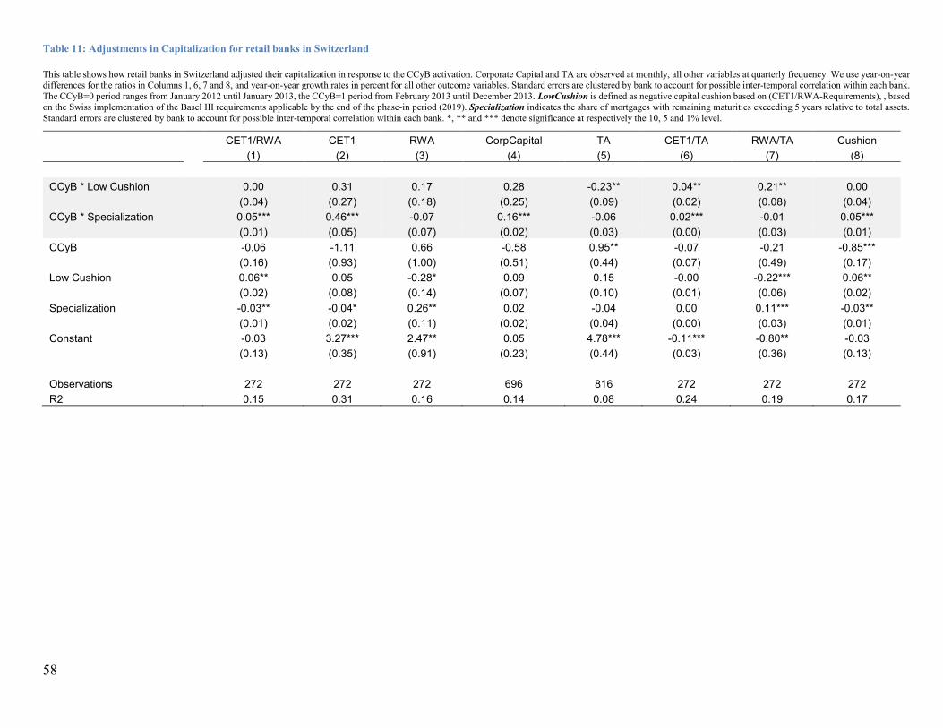
58
Table 11: Adjustments in Capitalization for retail banks in Switzerland
This table shows how retail banks in Switzerland adjusted their capitalization in response to the CCyB activation. Corporate Capital and TA are observed at monthly, all other variables at quarterly frequency. We use year-on-year differences for the ratios in Columns 1, 6, 7 and 8, and year-on-year growth rates in percent for all other outcome variables. Standard errors are clustered by bank to account for possible inter-temporal correlation within each bank.
The CCyB=0 period ranges from January 2012 until January 2013, the CCyB=1 period from February 2013 until December 2013. LowCushion is defined as negative capital cushion based on (CET1/RWA-Requirements), , based on the Swiss implementation of the Basel III requirements applicable by the end of the phase-in period (2019). Specialization indicates the share of mortgages with remaining maturities exceeding 5 years relative to total assets.
Standard errors are clustered by bank to account for possible inter-temporal correlation within each bank. *, ** and *** denote significance at respectively the 10, 5 and 1% level.
CET1/RWA CET1 RWA CorpCapital TA CET1/TA RWA/TA Cushion
(1) (2) (3) (4) (5) (6) (7) (8)
CCyB * Low Cushion 0.00 0.31 0.17 0.28 -0.23** 0.04** 0.21** 0.00
(0.04) (0.27) (0.18) (0.25) (0.09) (0.02) (0.08) (0.04)
CCyB * Specialization 0.05*** 0.46*** -0.07 0.16*** -0.06 0.02*** -0.01 0.05***
(0.01) (0.05) (0.07) (0.02) (0.03) (0.00) (0.03) (0.01)
CCyB -0.06 -1.11 0.66 -0.58 0.95** -0.07 -0.21 -0.85***
(0.16) (0.93) (1.00) (0.51) (0.44) (0.07) (0.49) (0.17)
Low Cushion 0.06** 0.05 -0.28* 0.09 0.15 -0.00 -0.22*** 0.06**
(0.02) (0.08) (0.14) (0.07) (0.10) (0.01) (0.06) (0.02)
Specialization -0.03** -0.04* 0.26** 0.02 -0.04 0.00 0.11*** -0.03**
(0.01) (0.02) (0.11) (0.02) (0.04) (0.00) (0.03) (0.01)
Constant -0.03 3.27*** 2.47** 0.05 4.78*** -0.11*** -0.80** -0.03
(0.13) (0.35) (0.91) (0.23) (0.44) (0.03) (0.36) (0.13)
Observations 272 272 272 696 816 272 272 272
R2 0.15 0.31 0.16 0.14 0.08 0.24 0.19 0.17
Online Appendix
The purpose of this detailed Online Appendix is to provide more detailed background information.
Specifically, Section A1 describes the structure and setup of the Swiss residential mortgage
market, including the current regulatory standards for banks and borrowers. Section A2 informs
about the current set and recent changes of the capital requirements for banks. It also gives
references to the legal texts that exceed the scope of our main paper. Section A3 shows how
representative our sample is of the entire Swiss residential mortgage market. Finally, Section A4
sketches how loan prices can be decomposed in the dealership model of banking, a framework on
which we build the specification used for our analysis of how the CCyB affects mortgage pricing.
A1. The Swiss Mortgage Market
A1a. Low Rate of Owner-Occupied Residential Property
The CCyB as designed and implemented in Switzerland applies only to Swiss residential
mortgages. For this reason, we briefly introduce the Swiss real estate and residential mortgage
markets. Relative to other developed countries, Switzerland has always had a comparatively low
rate of owner-occupied residential property. At the national average, that rate was below one-third
until the early 1990s. Since then, it has risen to slightly above 40% given the possibility that home
buyers can use pension funds for their purchase of residential property and benefit from tax
incentives against the background of a low interest rate environment, especially during the more
recent years33.
A1b. Tax Treatment Incentivizing Slow Debt Repayment
The tax treatment is meant to be ownership neutral: Imputed rents are fully taxed also for owner-
occupants, while mortgage interest payments can be deducted from taxable income.34 This system
is in principle neutral to ownership, however it does create incentives for a very slow mortgage
amortization of residential mortgages. Hence Swiss households tend to amortize on a far longer
schedule than the contractual maturity of an individual single mortgage. They typically make the
balloon payment for outstanding principal at the end by refinancing, i.e. taking out a new loan. As
a consequence, Swiss mortgage debt has increased significantly during the recent boom. It is now
one of the highest in the world as a percentage of GDP (see FINMA, 2014), although most home
owners accumulate savings while keeping their mortgage debt outstanding.
33 Source: Bundesamt für Wohnungswesen, Wohneigentumsquoten 1990, 2000 und 2012 nach Kantonen,
http://www.bwo.admin.ch/dokumentation/
34 See IMF (2011). IMF (2011) also writes that Switzerland is the only country apart from the Netherlands to have this fully ownership neutral
tax regime.
60
A1c. Typical Maturities and Repayment Behavior
Swiss mortgage suppliers rarely offer contractual maturities above 10 years, although amongst
maturities below 10 years those with longer fixing of interest rates have become significantly more
popular in the low interest rate environment of the past few years.35 More than half of all submitted
mortgage applications in our data set request mortgages with interest rates fixed for 10 years. In
contrast to the US, for example, early repayments in Switzerland usually occur only when
households have to move, e.g. because of divorce or job changes. By contrast, borrowers do not
repay earlier for strategic reasons, as Swiss banks usually charge a substantial compensating fine
for the lost investment opportunity and all incurred costs.
A1d. Actors in the Swiss Mortgage Market
In Switzerland, both banks and insurance companies offer mortgages, although the insurers hold
only about 4% market share (see FINMA, 2014). Some pension funds do also offer mortgages, but
their market share is below that of insurers and their mortgage volume has in recent years been
declining even in absolute terms. In this paper we focus only on banks, as insurers did not need to
comply with the regulatory requirements of the CCyB, nor would they constitute an adequate
control group, since they do operate in the same market.
A1e. The Swiss Real Estate Cycle
Finally, looking at the Swiss residential property price cycle, Swiss house prices peaked at
around 1992, then they declined until about 1999, and have ever since been continuously growing
for the recent 15 years. As Basten and Koch (forthcoming) show in more detail, part of this boom
has likely been due to the low interest environment and the appealing business model of mortgage
lending for both banks and households. Increased immigration and the fact that demand for
residential property faces a relatively inelastic housing supply seem to have also contributed to
this growth.36,37
A1f. Relevant Regulation
The Capital Adequacy Ordinance (CAO) provides the regulatory framework of the mortgage
market during our sample period (see FINMA, 2013a). More detailed provisions are given by the
Swiss Bankers’ Association’s self-imposed regulatory standards (see SBA, 2011 and 2012). This
35 According to SNB (2014) the share of outstanding mortgage debt with a remaining maturity above 5 years increased from about 15% in 2009
to above 25% in 2014. And this 10 percentage point increase does still greatly underestimate that in the characteristics of recently granted mortgages, as the stock of mortgages on balance sheets adjusts only partly each year.
36 For other up-to-date portraits of the Swiss mortgage market, see Brown and Guin (2013).
37 For additional information on the Swiss mortgage market, see BCBS (2013) and IMF (2014)
61
set of self-imposed guidelines became a declared a minimum standard by the Swiss Financial
Market Supervisory Authority FINMA, (see FINMA, 2012a).
A2. Capital Requirements and Further Institutional Information on the CCyB
The Countercyclical Capital Buffer (CCyB) is imposed on top of other capital requirements
implied by the Basel Committee on Banking Supervision (BCBS)’s Capital Accords. We list these
other capital requirements below that do not change during our sample period. First, there is the
Minimum Capital Requirement (MCR) already in place under Basel II. It amounts to 8% of risk-
weighted assets (RWA) and its violation will automatically trigger regulatory action. Second, also
since Basel II, there are the bank-specific Pillar II requirements which depend on national
supervisors’ assessment of a bank’s riskiness. In Switzerland, the majority of these Pillar II
requirements depend on which out of five risk categories a bank has been assigned to. As explained
in Jans and Passardi (2013), the supervisor FINMA has assigned Swiss banks to five target and
intervention threshold groups depending inter alia on their balance sheet size. The capital
requirements specified by the respective risk category range from 2.5% to 6.4% of RWA. Hence,
depending on their actual idiosyncratic level of capitalization, two banks may have different capital
cushions in excess of the common category’s requirement that FINMA has assigned to them. These
category-based requirements are gradually phased in until 2019, yet we would expect their effect
on loan pricing to take effect at the latest by the time by which the new requirements have been
definitely decided on. Third, Basel III envisages also a Capital Conservation Buffer amounting to
2.5% of RWA, which may be temporarily violated in times of crisis. In Switzerland, ultimately
the first 2.5 percentage points of the category based requirements (the 2.5%-6.4% of RWA) will
count as Capital Conservation Buffer and hence Pillar I requirement, while the rest will continue
to count as Pillar II requirement. FINMA (2011), FINMA (2012b), FINMA (2013c) and Jans and
Passardi (2013) provide more details on the implementation of those different capital requirements
in Switzerland.
For more detailed institutional information on the CCyB, beyond those discussed in our paper, we
refer to BCBS (2010b), BCBS (2010c), SNB (2013a) and SNB (2013b). For a discussion on
appropriate metrics for timing the activation of the CCyB, see Borio et al. (2010), Borio et al.
(2011), Repullo and Saurina (2011), Edge and Meisenzahl (2011) and Hahm and Shin (2013).
A3. How Representative is the Comparis sample of the entire Swiss Mortgage Market?
To investigate how representative our dataset is of the overall Swiss mortgage market, we compare
our sample data to other micro-level and aggregate data from three available sources: First, we
draw on aggregate data capturing the entire Swiss market from the Swiss National Bank’s (SNB)
publication “Banks in Switzerland”, SNB (2012). Second, we compare our estimation sample to
other micro data from the Household Budget Survey (HBS, or HABE), and third to another survey
dataset from a study by Seiler (2013) on households’ use of pension money for real estate
acquisitions. The SNB aggregate data cover a few characteristics of the stock of all mortgages
listed on Swiss banks’ balance sheets. The drawback of this dataset however is, that it does not
allow us to compare these characteristics specifically of those of mortgages that have only recently
62
been granted as new or rollover mortgages during our relevant period of time (July 2012 to October
2013). As opposed to that, the HBS and Seiler (2013) datasets allow us to focus more closely on
recently made mortgages, but the HBS covers only few characteristics, and the survey data from
Seiler (2013) may themselves not be fully representative of the entire market in all respects. To
the best of our knowledge, these are the only suitable public data sources and taken together they
can give the best possible idea of how our sample compares to the Swiss mortgage market as a
whole. We structure the following discussion around the three dimensions along which the data
allow for useful comparisons: Location of the underlying real estate object, the loan-to-value
(LTV) ratio implied by the requested mortgage amount, and key figures on the requesting
households’ finances.
A3a. Location
Our first question is how well our sample covers Switzerland’s different regions. To account for
time-invariant heterogeneity across the property’s location in our regression analysis, we use either
canton fixed effects or request fixed effects that are in turn nested by cantons. Despite these fixed
effects, the number of observations along the offer dimension (recall that there are multiple offers
per individual requests) might not be representative and thus our regression estimates might suit
some distinct areas but not Switzerland as a whole. We hence compare the geographical
distribution of the observations in our sample to those implied by SNB (2012) and Seiler (2013).
Panel (A) of Table A1 shows the comparison of our sample with the SNB data which are available
at the level of the 26 Swiss cantons (federal states). Following the SNB statistics, we compute the
share in terms of the volume of extended mortgages by canton of the residential property relative
to the volume of all extended mortgages in Switzerland. In this way, Column (1a) relies on
aggregate data and features these shares while sorting the cantons by rank order based on the entire
Swiss market. By contrast, Column (2a) and (2b) draw on our estimation sample. Column (2a)
gives the share of requested mortgage volumes by locational canton and Column (2b) gives the
share’s rank according. The last two Columns replicate the share and its rank in our sample but
draw on the un-weighted average of the number of requests instead of implicitly weighting by
requested mortgage amounts as in previous columns. These figures show that our sample is quite
representative, covering not only the most densely populated cantons like Zurich, but also the more
rural areas. More formally, we can compute the χ2 statistic to test the null hypothesis that both
figures represent the same underlying distribution. Doing so yields test statistics between 5 and 6,
depending on whether we look at the volume or number of requests. These values are far below
the relevant critical values to reject the null (starting from about 34 for 25 degrees of freedom), so
we can conclude that our sample has no geographical bias relative to the entire Swiss mortgage
market.
In Panel (B) of Table A1 we reduce our sample to the 7 distinct market regions to align it with the
Seiler (2013) survey data. This survey dataset might itself not be representative of the entire Swiss
market, yet we found a more focused comparison also quite informative. The comparison shows
that we have a slightly higher coverage of French- and Italian- (as opposed to German-) speaking
Switzerland, thus alleviating further possible concerns that our sample might give too much weight
to German-speaking Switzerland.
A3b. Loan-to-Value (LTV) Ratios
63
Table A2 compares the Loan-to-Value (LTV) ratios in our sample to those in the two other
available data sources. Panel (A) starts with the SNB data, noting the drawback that these cover
the stock of all mortgages on banks’ balance sheets, including those granted in past years. Since
SNB data give the fractions of mortgage volumes in 3 different LTV buckets, we compute the
same distribution for our data. With regard to the entire Swiss mortgage market, we find that about
92.4% of all issued mortgages fall into the lowest LTV bucket below 67%. This compares well
with our sample, in which 91% of all requested mortgages fall into this bucket. As to more risky
mortgages in the medium category of LTV ratios above 67% but below 80%, data on the entire
Swiss market point out that 5.7% populate this bucket. In our sample, 8.2% of all mortgages
populate that medium bucket. The top bucket ranges from LTVs above 80% to 100%. It is filled
by 1.9% of the entire Swiss market, whereas only 0.8% of our sample fills this bucket. We attribute
these small differences in the most risky buckets to the fact that data on the entire Swiss market
unfortunately are only available for the entire stock of all mortgages granted by banks over time
and not for our relevant period in specific. In fact, our sample focuses on mortgage requests
submitted after July 2012 when stricter rules on LTV ratios above 80% and tighter rules on
household equity had become effective. Panel (B) compares mean and median LTV in our sample
to those in Seiler (2013). Here, we do not find a significant difference: In our sample the mean
(median) LTV of new mortgage requests amounts to 69 (74), whereas in Seiler (2013) it amounts
to 71 (74).
A3c. Household Finances
Looking at household finances, our summary statistics in the top panel of our main paper’s Table
3 show a median gross annual household income of CHF 155’000 and median household wealth
of CHF 313’000. At first sight, these numbers may seem very high, but to put them into
perspective, one needs to take the Swiss price and income levels into account. For our purpose, a
comparison with figures from other Swiss data sources lends support to our sample dataset.
Unfortunately the SNB (2012) data aggregates are based on banks’ balance sheets and hence
contain no information on property buyers’ income or wealth, and Seiler (2013) contains data on
personal wealth only from the year of the survey as opposed to the year of the purchase. However,
the Household Budget Survey has data on household incomes (albeit not on wealth). This micro-
level survey data tells us that while the gross annual income of all households surveyed amounts
to only CHF 133’000 on average, that of the average home-owner starts at CHF 150’000 and may
be as high as CHF 177’000 with 3 or more children. Since households are typically aged below 65
when purchasing their residential property, we consider the latter set of values more relevant. We
conclude that income levels of the households in our sample are within the normal range for Swiss
home-owning households.
Overall we infer from these figures and comparisons, that our sample in terms of geographical
distribution and borrower characteristics seems to be quite representative of the entire Swiss
mortgage and residential property market.
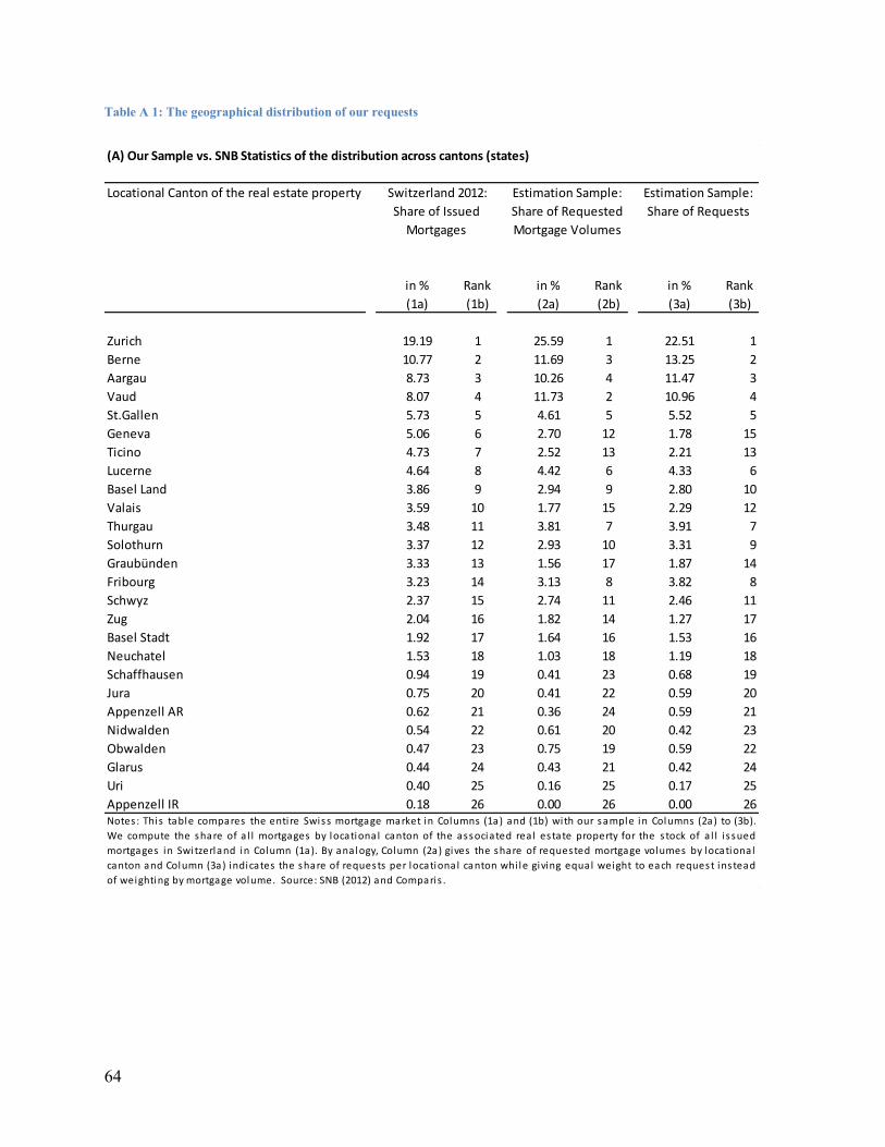
64
Table A 1: The geographical distribution of our requests
in % Rank in % Rank in % Rank
(1a) (1b) (2a) (2b) (3a) (3b)
Zurich 19.19 1 25.59 1 22.51 1
Berne 10.77 2 11.69 3 13.25 2
Aargau 8.73 3 10.26 4 11.47 3
Vaud 8.07 4 11.73 2 10.96 4
St.Gallen 5.73 5 4.61 5 5.52 5
Geneva 5.06 6 2.70 12 1.78 15
Ticino 4.73 7 2.52 13 2.21 13
Lucerne 4.64 8 4.42 6 4.33 6
Basel Land 3.86 9 2.94 9 2.80 10
Valais 3.59 10 1.77 15 2.29 12
Thurgau 3.48 11 3.81 7 3.91 7
Solothurn 3.37 12 2.93 10 3.31 9
Graubünden 3.33 13 1.56 17 1.87 14
Fribourg 3.23 14 3.13 8 3.82 8
Schwyz 2.37 15 2.74 11 2.46 11
Zug 2.04 16 1.82 14 1.27 17
Basel Stadt 1.92 17 1.64 16 1.53 16
Neuchatel 1.53 18 1.03 18 1.19 18
Schaffhausen 0.94 19 0.41 23 0.68 19
Jura 0.75 20 0.41 22 0.59 20
Appenzell AR 0.62 21 0.36 24 0.59 21
Nidwalden 0.54 22 0.61 20 0.42 23
Obwalden 0.47 23 0.75 19 0.59 22
Glarus 0.44 24 0.43 21 0.42 24
Uri 0.40 25 0.16 25 0.17 25
Appenzell IR 0.18 26 0.00 26 0.00 26
Switzerland 2012:
Share of Issued
Mortgages
Estimation Sample:
Share of Requested
Mortgage Volumes
Estimation Sample:
Share of Requests
Notes : This table compares the entire Swiss mortgage market in Columns (1a) and (1b) with our sample in Columns (2a) to (3b).
We compute the share of a l l mortgages by locational canton of the associated real estate property for the stock of a l l i s sued
mortgages in Switzerland in Column (1a). By analogy, Column (2a) gives the share of requested mortgage volumes by locational
canton and Column (3a) indicates the share of requests per locational canton whi le giving equal weight to each request instead
of weighting by mortgage volume. Source: SNB (2012) and Comparis .
(A) Our Sample vs. SNB Statistics of the distribution across cantons (states)
Locational Canton of the real estate property
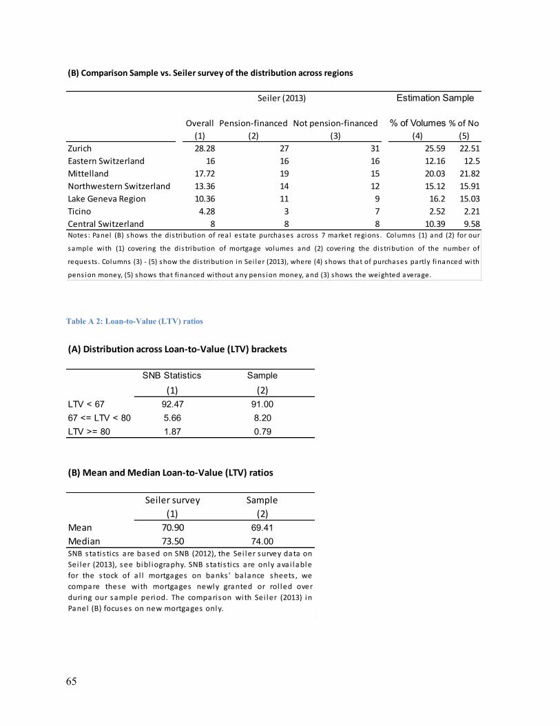
65
Table A 2: Loan-to-Value (LTV) ratios
Overall Pension-financed Not pension-financed % of Volumes % of No
(1) (2) (3) (4) (5)
Zurich 28.28 27 31 25.59 22.51
Eastern Switzerland 16 16 16 12.16 12.5
Mittelland 17.72 19 15 20.03 21.82
Northwestern Switzerland 13.36 14 12 15.12 15.91
Lake Geneva Region 10.36 11 9 16.2 15.03
Ticino 4.28 3 7 2.52 2.21
Central Switzerland 8 8 8 10.39 9.58Notes : Panel (B) shows the distribution of real estate purchases across 7 market regions . Columns (1) and (2) for our
sample with (1) covering the distribution of mortgage volumes and (2) covering the distribution of the number of
requests . Columns (3) - (5) show the distribution in Sei ler (2013), where (4) shows that of purchases partly financed with
pens ion money, (5) shows that financed without any pens ion money, and (3) shows the weighted average.
(B) Comparison Sample vs. Seiler survey of the distribution across regions
Seiler (2013) Estimation Sample
SNB Statistics Sample
(1) (2)
LTV < 67 92.47 91.00
67 <= LTV < 80 5.66 8.20
LTV >= 80 1.87 0.79
Seiler survey Sample
(1) (2)
Mean 70.90 69.41
Median 73.50 74.00
(B) Mean and Median Loan-to-Value (LTV) ratios
SNB statis tics are based on SNB (2012), the Sei ler survey data on
Sei ler (2013), see bibl iography. SNB statis tics are only avai lable
for the stock of a l l mortgages on banks ' ba lance sheets , we
compare these with mortgages newly granted or rol led over
during our sample period. The comparison with Sei ler (2013) in
Panel (B) focuses on new mortgages only.
(A) Distribution across Loan-to-Value (LTV) brackets
66
A4. Decomposing the Mortgage Interest Rate with the Dealership Model
As our key outcome variable of interest is the price of the mortgage, we build on the classic
dealership model originated by Ho and Saunders (1981), which was extended more recently by,
amongst others, Saunders and Schumacher (2000) and Maudos and Fernandez (2004). In this
mark-up pricing framework, banks set a loan rate rL at a spread above the prevailing wholesale
market funding rate r. This wholesale rate is also the rate at which any deposits that are not needed
to fund bank lending would be invested, which corresponds to the opportunity cost of lending. The
mark-up, in turn, can reflect a variety of factors. While Ho and Saunders (1981) focus only on
interest rate risk, Maudos and Fernandez (2004) point out theoretically =and empirically that the
spread above the wholesale rate is increasing not only in interest rate risk, but also in credit risk.
Furthermore, the loan rate is increasing in a bank’s capitalization level, although Maudos and
Fernandez interpret capitalization merely as a proxy for a bank’s risk aversion. By contrast,
Saunders and Schumacher (2000) point out that banks may choose higher capital ratios not only
because of economic risk aversion, but also to comply with regulatory requirements (like the
CCyB). For our setup this implies the following loan pricing equation:
ijijiij residualbankriskcreditswaprateloanrate (A)
In equation (A) above, swap rate and credit risk are captured by the request and the time-invariant
component of the bank residual by the bank fixed effect. In equation (A) the first two are being
controlled for explicitly. This allows us to identify separately the effect of the CCyB, which in the
dealership model would be subsumed under the time-variant component of the bank residual.
Having thus explained our estimation strategy, possible challenges to identification and the
rationale for our main dependent variable of interest, we can now turn to the results.