The Costs of Right of Way Acquisition: Methods and Models for Estimation

Jared D. Heiner Graduate Student Researcher

Department of Civil Engineering The University of Texas at Austin ECJ 6.204, Austin, Texas 78712,

Tel: (512) 232-4254 Email: jheiner@mail.utexas.edu

Kara M. Kockelman

(Corresponding Author) Clare Boothe Luce Assistant Professor of Civil Engineering

The University of Texas at Austin ECJ 6.904, Austin, Texas 78712,

Tel: (512) 471-4379 FAX: (512) 475-8744

Email: kkockelm@mail.utexas.edu The following paper is a pre-print and the final publication can be found in Journal of Transportation Engineering 131 (3):193-204, 2005. Presented at the 83rd Annual Meeting of the Transportation Research Board, January 2004.

ABSTRACT Transportation infrastructure and other major projects often require the taking of real property, or right-of-way (ROW). The costs of partial takings, commercial properties, remainder damages, court costs, utility relocations, and other ROW-related items are difficult to anticipate. Accurate estimation procedures are needed to facilitate budgeting and timely completion of projects.

This paper reviews the literature related to ROW acquisition and property valuation. It describes the appraisal process and the influence of federal law on acquisition practices. It provides hedonic price models for estimation of costs associated with taking property using recent acquisition data from several Texas corridors and full-parcel commercial sales transactions in Texas’ largest regions. Results indicate that damages depend heavily on parking, access, and location, the size of the taking is not as important as the value of improvements, and utility costs are highly variable.

Key Words: Right of Way Acquisition, Property Valuation, Cost Estimation, Commercial Real Estate

Jared D. Heiner and Kara M. Kockelman 2

INTRODUCTION

This paper examines the difficulties and challenges associated with ROW cost estimation. Emphasis is placed on projects in metropolitan areas and the treatment of commercial properties. In order to identify specific challenges, ROW administrators and other real estate professionals were interviewed, and a survey of the literature and research related to ROW acquisition and property valuation was performed. The literature studied addresses formal procedures required of ROW acquisition on federal projects, property appraisal methods, and the effects of transportation improvements on property values. Among this latter research, studies of home prices are plentiful, but very few studies of commercial properties or actual ROW purchases have been done. To fill this void in the literature, ROW purchase data and commercial sales data for Texas’ major metropolitan areas were gathered from several sources. These include the Texas Department of Transportation (TXDOT), the Travis Central Appraisal District (TCAD, serving the central Austin area), and the CoStar Group, a national provider of commercial sales data for metropolitan areas. A total cost model was developed for the ROW purchase data, and price models were developed for the commercial sales data, which provide predictions of land and improvement values for commercial properties. The data assembly and model estimation are discussed later in the paper.

BACKGROUND AND LITERATURE REVIEW

Right of way (ROW) acquisition for highway and transportation projects can be very expensive and time consuming. The federal government spent nearly one billion dollars for ROW in fiscal year 1999, at an average federal cost of $36,400 per parcel (FHWA, 2003). States and local agencies spent $1.8 billion in the same year, on projects subject to federal acquisition regulations. An additional $100 million in federal and state funds was paid to displaced business and property owners for reestablishment and relocation assistance (FHWA, 2003). The federal totals represent approximately 4 percent of total federal funding for highways in 1999 (AASHTO, 2002). Accurate ROW cost estimation can be key to project budgeting and completion. Texas ROW administrators report a number of challenges routinely encountered in ROW cost estimation (Kockelman, et al., 2003). First, early estimates are based on planning-level maps, so project administrators must anticipate the extent of takings based on limited information. Second, administrators often have limited time to prepare estimates, thus restricting the amount of research that can be undertaken for complex parcels. Third, they typically prepare ROW estimates several years in advance of actual ROW acquisition, during which time significant inflation and speculation can occur, resulting in property and damage appreciation. Administrators (both urban and rural) report that this time interval is typically three years, but it may stretch to seven years in some cases (Kockelman, et al., 2003). These factors can easily combine to bias ROW cost estimates low. In addition to these challenges, ROW professionals cite uncertainties associated with damages and court costs as obstacles to accurate estimation (Please see Table 1 for a definition of key terms). ROW acquisition involves partial takings, which may damage the remainder. Common damages include loss of parking, which compromises the use intensity of the remainder, loss of visibility, which compromises the value of signage, and restriction or removal of access. The value of such damages is often difficult to predict, and can be a source of substantial estimation error. Moreover, court costs are highly variable, and are particularly high for projects in highly developed commercial corridors, where condemnation proceedings are common. Condemnation awards can add significantly to the total cost of acquisition; ROW cost estimators in metropolitan areas routinely add from 25 to 40 percent to the projected base cost of acquisition, in anticipation of these costs (Kockelman, et al., 2003) In cases where access rights are removed, such as in the upgrade of public highways to controlled-access freeways, property owners are entitled to compensation. Kockelman, et al. (2002) calculated a range of access costs using data from Westerfield’s (1993) and Gallego’s (1996) regression models for Texas settlements. Access costs ranged from $0 to $2,490 per linear foot of frontage, with an average value of $511 per linear foot1. They suggested that proactive access management and corridor preservation strategies may reduce future damages arising from loss of access. Of course, transportation agencies must be very careful to avoid preemptive takings, wherein land use rights are prematurely restricted, in long-term anticipation of projects involving ROW acquisition (FHWA, 2000, Sneckner, 2002). The shape, access, and other characteristics of property remainders resulting from partial takings may warrant a reduction in the property’s highest and best use. Using surveys of public and private experts and regression analyses of historical ROW cost data for the State of Texas, Buffington, et al. (1995) identified key characteristics of remainders. Their survey responses suggested that the most significant variables affecting acquisition cost for partial takings are the size and shape of the remainder, reductions in the highest and best use,

Jared D. Heiner and Kara M. Kockelman 3

location of remaining access points, and length of remaining frontage. Their regression results indicated that commercial properties increase the total taking cost by $24,000 per acre, compared to other land uses. The shape of the remainder was also significant: a rectangular remainder reduced the total taking cost by nearly $12,000, compared to other, odd shapes. Aside from property acquisition costs, transportation professionals must estimate the budget impact of utility relocations. These costs can run very high, and may even exceed property acquisition costs. For example, current cost estimates for utility relocations required in the expansion of Interstate 10 in Houston, Texas, exceed $200 million (Kockelman, et al., 2003). This represents a unit cost of $10 million per mile for this 20-mile stretch of roadway, or 30% of the ROW budget.

The Uniform Act and Property Appraisal

In addition to ROW costs and uncertainties, there are many formal ROW procedures required of transportation agencies. The federal Uniform Act establishes standards and guidelines for real property acquisition on projects which receive federal funds (or federal assistance) for any project phase or task. Its purpose is to provide for the fair treatment of property owners where real property must be taken for any federal (or federally-assisted) project. Its procedures seek to “expedite acquisition, avoid litigation, and establish confidence in federal land acquisition practices.” (49 CFR 24) It requires the acquiring agency offer the property owner “just compensation”, based on an independent appraisal of fair market value. Formal property appraisals play a key role in the final determination of individual property values, and therefore in the final determination of parcel-specific ROW costs. The most common and accepted valuation method is the sales comparison approach, which requires access to recent and relevant arms-length sales data. Other accepted valuation methods include the income and the cost approaches (FHWA, 2002a, Wurtzebach and Miles, 1991). The income approach may be used for commercial or investment properties, by considering gross rent, vacancy rates, and typical operating expenses, in order to estimate net income. The cost approach evaluates the replacement cost, and subtracts depreciation or obsolescence of the existing structure. This last approach is only used in cases where special purpose improvements develop the property to its highest and best use (FHWA, 2002a). In addition to being the most common and accepted method, the sales comparison approach is generally the easiest method to use. Comparable sales, listings, or rental data may be obtained from appraisal districts, title companies, private appraisers, and/or online data services. This method is most helpful in assessing the value of single-family residential properties and raw land, where sales data are plentiful (Wurtzebach and Miles, 1991). Sales data for commercial properties are relatively limited and more difficult to obtain (Carey, 2001, Gatzlaff and Geltner, 1998). This research enhances the literature by providing predictions of commercial property values, based on a large sample of commercial sales transactions for Texas’s major metro areas. These data are described in the Data Assembly section.

Enhanced Value: Research and Models

The effect of highway construction on property values has been studied by many, using statistical regression tools. Ten Siethoff and Kockelman (2002) estimated land, and improvement value models to determine the effects of the expansion of US 183 in Austin, Texas on commercial property values between 1982 and 1999. Land values were estimated to fall $52,000 per acre one-half mile from the facility, compared to lots that fronted the new facility. Corner lots at signalized intersections were valued $55,000 higher per acre, and their built improvements $4.61 higher per square foot. Thus, location and access characteristics can be strong determinants of property value. And transportation projects can dramatically enhance land and improvement values. In another study, Vadali and Sohn (2001) employed hedonic models to examine variation in home sales prices along the North Central Expressway (NCE) in Dallas, Texas from 1979 to 1997. They obtained sales data for residential properties from a private tax database and Dallas County Appraisal District records, then used GIS tools to distinguish spatial data and code location and environmental variables. A light rail transit line was constructed in the NCE ROW simultaneously with the roadway improvements. Comparison of corridor house prices with hedonic property value indices for Dallas2 revealed significant price effects of the corridor improvement phases. During the pre-planning phase, housing prices in the immediate vicinity of the freeway were negatively affected, while those further away were positively affected. During the planning phase, houses in the corridor appreciated at twice the rate of other Dallas properties. Prices declined more rapidly than those elsewhere in Dallas during the early construction phases (from 1987-1994). However, prices again improved during the final construction phase, as sections of the freeway began to reopen, and access improved.

Jared D. Heiner and Kara M. Kockelman 4

Carey (2001) studied the impacts from the construction of the Superstition Freeway (US60) on adjacent land uses and home values in Phoenix, Arizona3. He obtained repeat sales data through a local title company, in order to make paired sales comparisons and perform time-series regression for the twenty-year period from 1980 to 2000, for both single-family detached homes and condominiums/townhouses. The results revealed that homes less than one-half mile from the freeway were negatively impacted, based on reductions in sales prices and lower appreciation rates, compared to homes greater than one-half mile from the facility. His study of condominiums/townhouses explained less variation in prices (R2 =0.646 vs. R2=0.795 for single-family homes) but suggested that buyers of condominiums and townhomes place a higher premium on access to major streets and freeways, than those buying single-family homes. Haider and Miller (2000) studied the effects of transportation infrastructure and location on real estate values for the Greater Toronto Area, using housing sales data from the Toronto Real Estate Board and census data. The data were spatially coded to create location variables for proximity to highways, subways, waterfront, and malls. Their study found that structural characteristics and neighborhood attributes, such as the average household income, are strong predictors of housing values, while proximity to transportation facilities explained less variation in housing values. Like Kockelman (1997), they recognized that the distance from the central business district (CBD) can be a very strong predictor of property values (even in the presence of far more sophisticated measures of accessibility), with home prices following a negative exponential trend with increasing distance from the CBD. Many real estate journals and other sources were searched for studies of commercial property prices. Gatzlaff and Geltner (2000) applied repeat sales regression techniques to estimate a commercial property price index for Florida, using transaction prices obtained from property tax records. They compared their results with the appraisal based National Council of Real Estate Investment Fiduciaries Florida Index, and found little difference in overall performance.

In addition to models of private transactions, some data sets and one or two formal models have been developed to assist ROW cost estimation for use by public transportation agencies. Several public agencies and their private consultants4 have developed databases to track ROW acquisition tasks and project costs. For example, the TXDOT implemented a ROW information system (ROWIS) in 1997, and Bentley Transportation recently developed a system for the Indiana DOT (ITE, 1999). Both the Indiana DOT and the TXDOT software use a relational database, and have the ability to monitor different acquisition functions and provide user level identification and access. However, they are limited in the variables they track, and they do not provide a model for prediction. The Virginia DOT recently developed a cost estimation model that includes ROW and utility components (VTRC, 2003).

As evident from the preceding discussion, models of home prices are plentiful, but few have developed models for commercial properties. And those of ROW acquisition costs are almost unheard of. This work addresses both of these limitations through acquisition and analysis of actual partial and full property purchases, for public roadway projects and via purely private transactions. DATA ASSEMBLY The data acquired here address the glaring gaps in the literature in the areas of commercial and ROW property appraisal. ROW purchase data were collected from the TXDOT and commercial sales data for Texas’ major metropolitan areas were gathered from the TCAD, and the CoStar Group. More detail on each of these data sets is provided below.

Texas Corridors

Historical ROW cost data were obtained from the TXDOT ROW Information Systems (ROWIS), which includes maps, costs, and parcel detail for roadway projects areas around the state. Most of the acquisition for the selected projects occurred recently (after 1997), so much of the cost and parcel information was available in the ROWIS database. ROW administrators suggested projects in Abilene, Corpus Christi, El Paso, Fort Worth, Houston, and San Antonio for study. The projects generally required the purchase of additional ROW necessary for the widening and expansion of existing facilities. Combined, the projects included over 20 centerline miles of highway, represented nearly $70 million in total acquisition costs, and yielded 285 parcels for detailed study.

More specifically, the Abilene project involved improvements to FM 604 (The FM designation is used for state routes in Texas), and consisted largely of takings of single family homes in the county. The Corpus Christi project consisted of an expansion of an existing two-lane highway (FM 1889) to a 4-lane facility, located approximately 20 miles from the city center, and included a number of agricultural parcels. The El Paso project widened the city’s North Loop (FM 76), and provided the greatest diversity in land uses among the projects. The Fort Worth project was a widening of East Rosedale Street, a major arterial. The Houston project consisted of a

Jared D. Heiner and Kara M. Kockelman 5

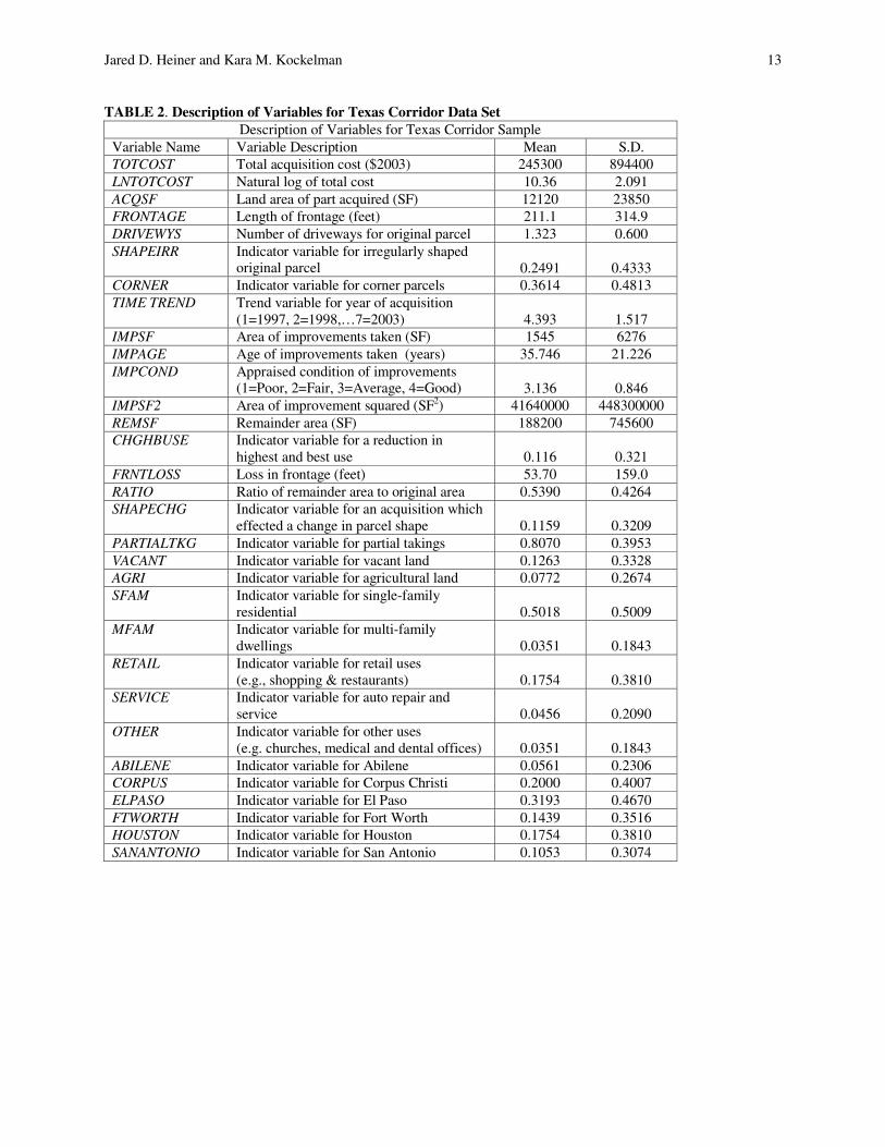
one-mile section of Interstate 10, a small part of a larger project. The majority of the Houston parcels were whole takings of homes, though the sample did capture several million-dollar commercial acquisitions. The San Antonio project involved a 6-mile section of US 281, and involved a high percentage of commercial properties. Information on the total cost paid, land values, improvement values, and the value of damages was exported from the ROWIS database, and dollar figures were adjusted for inflation using the Consumer Price Index (CPI) published by the U.S. Bureau of Labor Statistics (BLS, 2003). ROWIS also provided the use type, date acquired, and the method of acquisition for each parcel. Additional parcel detail was obtained from appraisal reports and ROW plans.5 Frontage and shape were measured for the original property, the acquired parcel, and the remainder, to identify changes in these important value determinants. Descriptions of variables and associated statistics for the Texas Corridors data are given in Table 2. Estimation of a log-log model is described later in the paper and regression results are reported in Table 3.

TCAD Commercial Sales Data – Travis County

A database of commercial sales transactions and property information was obtained from the TCAD, which actively seeks sales data6 in order to 100-percent (by law) appraise private real property for local tax collection. The database contained 1,354 commercial sales transactions that occurred between January 2000 and January 2003. Dollar values were corrected for inflation using the CPI (BLS, 2003). The TCAD database included information on lot size, improvement square footage, condition (or “grade”) of improvements, and year of construction. The properties were coded into land use classes according to the structure improvement code assigned by the Appraisal District. The geographic area codes used by the District were coded into location indicator variables7. An indicator variable was used for cases where the “list price” (i.e., the asking price) was substituted for the sales price. A full description of variables, land use classes, and location indicator variables for the TCAD commercial sales price model is given in Table 4. Regression results are shown in Table 5.

CoStar Commercial Sales Data – Texas’ Metropolitan Regions

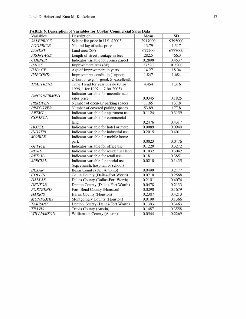
A database of commercial sales transactions was obtained from the CoStar Group (a national private provider of commercial real estate information) for the Austin, Dallas-Fort Worth, Houston and San Antonio metropolitan areas. The data set is more extensive than the TCAD database, in both size and detail and regional extent. The initial database contained over 24,000 records of commercial property transactions, but only 10,987 observations had documented sales prices. These represented $43.2 billion in total sales and spanned a 7-year time period, from June 1996 to June 2003. The sales prices were again adjusted for inflation using the CPI index (BLS 2003). The database contained information on lot and improvement size, land use, location, year of construction, and condition of improvements, along with number and type of parking stalls and frontage. An indicator variable was coded for unconfirmed sale prices, to see if these listings introduced bias in the model predictions. A full description of variables and associated statistics are shown in Table 6. Regression results are provided in Table 7.

MODEL ESTIMATION

Statistical regression models called hedonic price models are popular tools to estimate value (e.g., ten Siethoff and Kockelman, 2002, Vadali and Sohn, 2001, Carey, 2001, Haider and Miller, 2000, and Kockelman, 1997). These typically rely on structural characteristics, parcel size, and locational information. The models applied here follow work done by Kockelman (1997) and ten Siethoff and Kockelman (2002), wherein land and improvement areas are interacted with explanatory variables thought to influence land and structure values. In this way land rents per unit area can be distinguished. Models for each of the data sets are discussed briefly here now.

Total Cost Model for Texas Corridors

A cost of ROW acquisition per parcel model was developed using the TXDOT corridor data set. Each taken property’s total cost represents only the cost paid for land, improvements, damages and court awards; it does not include appraisal fees, personal or business relocation assistance, utilities, or other direct or indirect costs associated with acquisition. These also are real costs, and should not be overlooked in the preparation of estimates.

The total acquisition cost should be roughly the value of the taking plus damages. The value of the taking can be separated into the value of the land taken and the value of improvements taken (where applicable). Since land values should be fundamentally related to parcel size, the parcel size variable was interacted with a number of

Jared D. Heiner and Kara M. Kockelman 6

explanatory variables. Similarly, the improvement area was interacted with variables thought to influence the value of improvements. Of course, the value of some improvements is independent of the structure size; examples include fencing, signage, or other improvements. An attempt was made to code indicator variables in the model, for these takings; however, due to inconsistencies in reporting they were not used. Finally, damages may be associated with either the remaining land or remaining improvements. The general model form is shown here.

εβ

βββ

++

++=

∑

∑∑

kdamkdamk

jimpjimpj

ilandilandi

XREMSF

XIMPSFXACQSFTOTALCOST

),(

),(),,(

,

,0

where ACQSF is the size of the acquired parcel (in square feet), and Xi,land is a vector of explanatory variables related to the land value. They include a constant term, a land use indicator, a corner indicator, number of driveways, original frontage length, original parcel shape, location indicators, and the year of acquisition. IMPSF is the square footage of any structures that were acquired, and Xj,imp is a vector of explanatory variables linked to the structure’s value, such as use type, age, and condition. REMSF is the area of the remainder parcel in square feet, and Xk,dam is a vector of explanatory and indicator variables associated with damages to the remainder (e.g., a reduction in the highest and best use, a change in the parcel shape, the loss of frontage in feet, and the ratio of the remainder size to the original parcel size). Of course, ε is an error term, capturing the effects of unobserved/unrecorded variables, and recognizing that no model of such data can provide perfect predictions. A variety of explanatory variables and model forms were tested, in order to discover important interactions. A log-log model was chosen, which used the natural log of the total acquisition cost as the dependent variable, and log transformations of all explanatory variables. A conditional transformation was used to handle zero values, and retain indicator variables and their interactions in the model. Due to the small sample size, a threshold p-value of 0.25 was used to test variable significance and develop the final model specification. Removed variables were reintroduced separately to check for possible, later significance.

Sales Price Model for TCAD Commercial Sales

The model proposed for the TCAD commercial sales data is similar, except damages do not apply, and the market sale price was used as the dependent variable. The model form follows here:

εβ

βββ

++

++=

∑

∑∑

jimpjimpj

jimpjimpj

ilandilandi

XIMPSF

XIMPSFXLANDSFSALEPRICE

),(

),(),,(

,2

,0

where LANDSF is the parcel area in square feet, Xi,land is a vector of explanatory variables related to the land value (i.e., a constant term, land use indicator variables, area indicator variables, and list price), IMPSF is the square footage of improvements, Xj,imp is a vector of explanatory variables linked to the improvement value (e.g., age, condition, and use type), and ε is the error term. The square of the improvement area was interacted with use type indicator variables to recognize diminishing marginal returns for different properties. A list price indicator (to distinguish these observations from true, sale price) was tried independently, but then kept interacted.

Price Model for CoStar Commercial Sales Data

The model proposed for CoStar commercial sales data again used the market sales price as the dependent variable. A quadratic term was not used in the CoStar model. Parking spaces were considered separately in the model, in order to predict the value of individual parking spaces. The general model form for the CoStar commercial sales data is shown here:

ε

βββ

+++

+++= ∑∑

DUNCONFIRMEPRKOPEN

PRKCOVERXIMPSFXLANDSFSALEPRICEj

impjimpji

landilandi ),(),,( ,0

Jared D. Heiner and Kara M. Kockelman 7

where the LANDSF and IMPSF are as defined previously, PRKCOVER is the number of covered parking spaces, PRKOPEN is the number of uncovered parking spaces, UNCONFIRMED is an indicator variable for sale prices that were not confirmed, and ε is the error term.

Variance Model and Feasible Generalized Least Squares Estimation

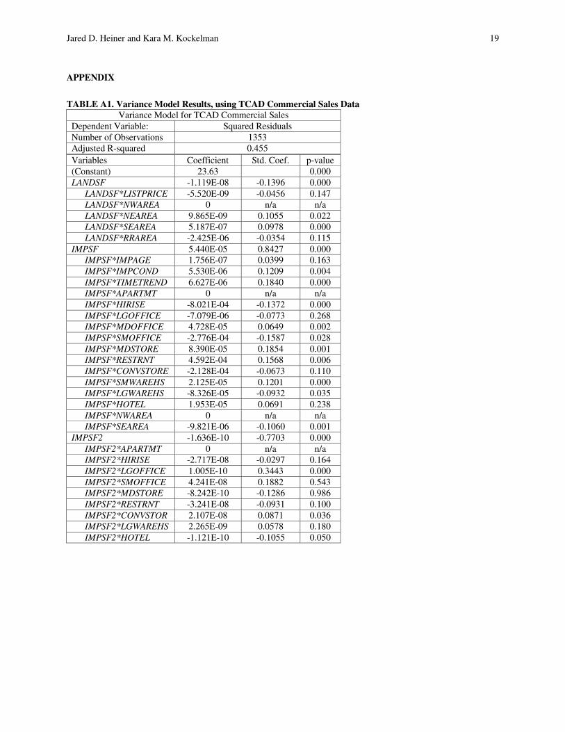
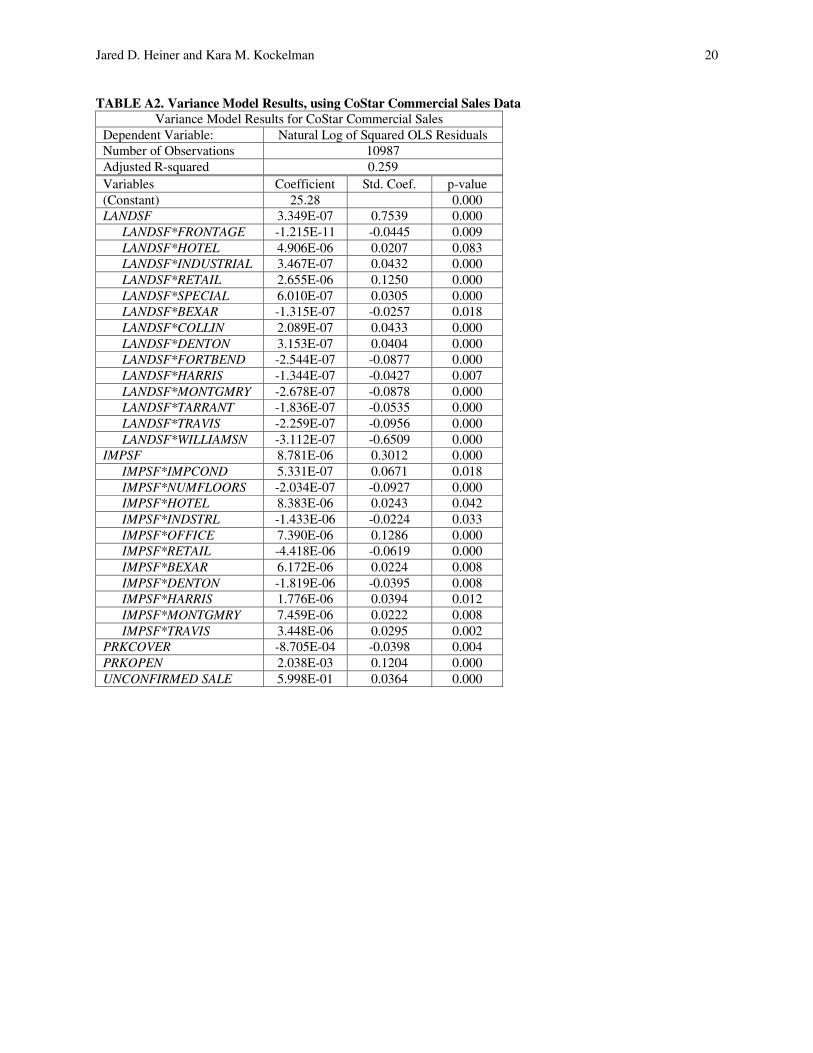
Variance models were performed for all data sets, to identify heteroskedasticity, a non-constant variation across observations. The variance models regressed the squared residual terms (obtained from initial OLS models) on the set of explanatory variables. In order to preclude negative variance predictions, an exponential variance model was used. The log-variance model for the TCAD sample returned an adjusted R-squared value of 0.453, and the CoStar data returned an adjusted R-squared value of 0.259, allowing one to reject the null hypothesis of homoskedasticity in both cases8. The variance model results for the TCAD and CoStar data are included in the Appendix.

FGLS regression was applied to the TCAD and CoStar commercial sales data to correct the estimates for the presence of heteroskedasticity, a non-constant variation across observations. In FGLS, one uses the inverse of the variance model predictions as weights in the regression. FGLS produces more efficient estimates for models where the data is known to be heteroskedastic. Another advantage is that FGLS does not require any underlying assumptions about the error terms’ distribution.

ANALYSIS AND RESULTS

The estimated coefficients, standardized coefficients, and p-values are provided in Tables 3, 5, and 7, for the Texas Corridors, Travis County, and CoStar data sets, respectively. (Standardized coefficients describe how many standard deviations change in the response variable one can expect from one standard deviation change in the associated explanatory variable.) Final models were arrived at via a process of stepwise addition and deletion (of variables based on levels of statistical significance). There are substantial differences in the three data sets, as described above; but all have measures of land, improvement size, and age of structure. The results of these regressions prove quite interesting.

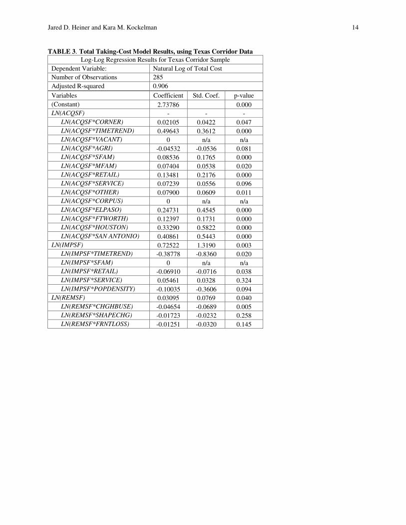
Total Cost Model for Texas Corridors

The data for the Texas corridors was analyzed using ordinary least squares regression, and the results of this analysis are in Table 3. The adjusted R-squared for the log-log model was 0.906. Log-log models are commonly used to measure the change in one variable in response the change in another. For example, the change in the total taking cost in response to an increase in the size of the taking. Several of the variables have significant effects on land value. Most notably, the time trend variable for the year of acquisition dominates this group of variables. The land use types are all statistically significant at the 0.10 level, with retail uses having the strongest effect on the total taking cost. This is consistent with the expectation that differences in value arising from land use should be linked to the land value. The location indicator variables were all retained in the final model, with the exception of Abilene. Abilene is perhaps the most similar in nature to Corpus Christi, which was used as the base case. Both of these projects occurred in the county, outside of city limits.

Approximately 40 percent of the parcels involved the taking of improvements. For these cases, the improvement area strongly influences the total taking cost. Only the coefficient for retail use is statistically significant among the improvement types, but its coefficient is negative. This result may offset the strong positive effect of retail use on land value. Specifications including variables for the distance to CBD, and average household income also were tried; the income and distance-to-CBD measures were helpful in explaining property values but may proxy for the area indicators to some extent, thus biasing the results.

Several of the variables associated with damages to the remainder are significant in the model. However, the estimated coefficients for these variables; change in the highest and best use, change in parcel shape, and reduction of frontage length are all negative, counter to one’s intuition. It may be that the high positive constant for the remainder parcel area is hiding the true effect of these variables.

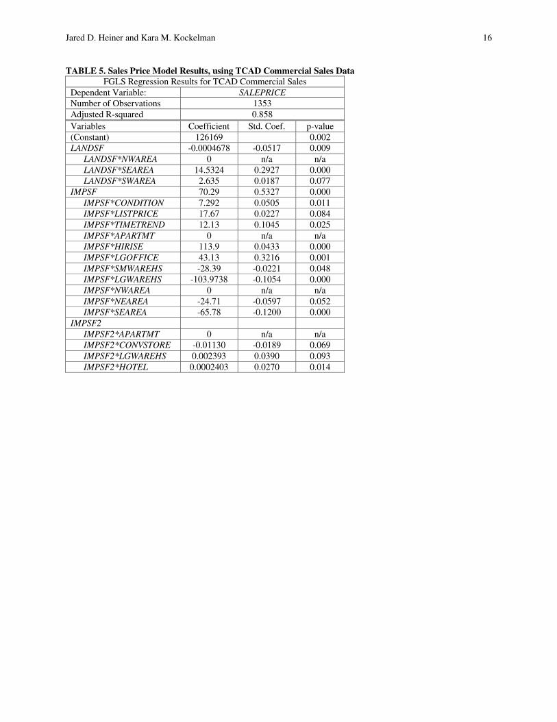
Price Model for Travis County Commercial Sales

A number of explanatory variables were tested for the TCAD commercial sales data, using sales price as the dependent variable. The adjusted R-squared for the FGLS model was 0.856, a significant improvement upon the OLS result (0.705), and very high for this type of analysis. FGLS regression results for the TCAD commercial sales data are shown in Table 5. Regarding land value, two location indicator variables are significant in the final model.

Jared D. Heiner and Kara M. Kockelman 8

Land in the southeast area, which includes downtown Austin, is predicted to have much higher value than other areas in the region9. The improvement area is a very strong predictor of value. The condition of the structure is both statistically and practically significant in the model; a property in excellent condition is worth approximately $22 more per square foot than a similar property in fair condition.

As expected, the list price indicator is positive and significant (suggesting that listing prices are higher than final sale prices). Several of the different use types have a marked effect upon the value of improvements. Hi-rise and multi-story office buildings hold the highest value, and industrial uses are valued less. The SE and NE location indicator variables are also significant, reflecting local variation in property values within Travis County. In theory, these location values should be reflected in the price of land, rather than improved area. However, with buildings enduring many decades, the structure itself may begin picking up these effects, since one cannot easily replace such buildings.

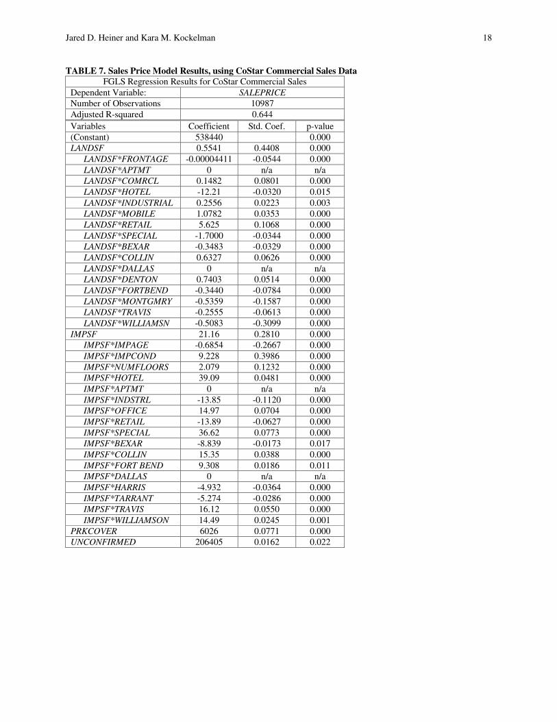
Price Model for CoStar Commercial Sales

The CoStar commercial sales data was also modeled using FGLS regression techniques. The final results for the CoStar model are shown in Table 7. The adjusted R-squared for the FGLS model was 0.644, which was lower than the initial OLS result (0.856). The CoStar data contained a number of observations with very high values, which probably biased the initial OLS estimates. The coefficient for the square footage of land is a very strong predictor of value, based on the high (very practically significant) standardized coefficient. Many of the land use and location indicator variables (when interacted with land area) are statistically and practically significant in the CoStar model. Retail uses are predicted to add the highest premium to the land, as one would expect. Many of the county indicators are both statistically and practically significant, reflecting regional differences in land values.

Improvement square footage is a strong predictor of value for developed properties. The coefficient for improvement age is negative, which is not as one would expect. The condition of the structure is again significant; a property in excellent condition is worth nearly $28 more per square foot of improvement than a similar property in fair condition, slightly higher than the result of the TCAD model. A number of the improvement types are statistically significant. The coefficient for industrial properties is again negative, relative to apartments. The coefficient for retail buildings is negative, however, this result may be tempered by the high land values for these types of properties. The count variable for surface parking was not significant in the final model, but covered parking spaces are predicted to add $6,000 each. This estimate is low; Litman (1999) reports structured parking costs at $11,000 per space, exclusive of land costs. The indicator variable for unconfirmed sales is positive, suggesting bias or recording errors for these unconfirmed sales.

CONCLUSIONS

This research presents valuable insights into the challenges to accurate ROW estimation. The three price models add significantly to the literature by presenting predictions of actual ROW purchase costs, along with those of full-parcel commercial-sales transactions. Results indicate a great many features of such property valuation. One that is particularly distinctive arises in full-property purchases, where improvements appear to capture much more of a property’s locational value than the land beneath it. Modelers should be wary of biases that can arise in hedonic models. Such biases may abound in weak data sets, and mystify modelers and model users. The method of FGLS was successfully used to correct the commercial sales estimates for heteroskedasticity.

These models should prove valuable to ROW professionals, transportation project planners, developers, appraisers, and others in cost estimation for ROW and other acquisitions, particularly when the parcels involve commercial property in metropolitan areas. The 10-county database used here, representing Texas’s top four metro regions, proved sufficiently detailed and extensive to serve as a helpful predictor of commercial property values. To demonstrate the application of these models to actual sites, an example of predictions for a 10-parcel corridor in Fort Bend County (Houston metro area) is provided in the Appendix. Such predictions could be used as part of a larger framework to develop a project cost estimate. However, the models do have their limitations. The models only provide predictions of land and improvement values, and limited analysis of damage values. A more thorough treatment of damages, condemnation costs, and utility relocation costs certainly could add to practice and to research. The commercial sales data represent whole takings, via private transactions, so they do not provide actual ROW acquisition costs for partial takings by public agencies. Finally, data outside of Texas and results based on more generic (less region-specific) variables would be helpful; these may be variables characterizing regional population, wages, climate, accessibility, and local amenities.

Jared D. Heiner and Kara M. Kockelman 9

The acquisition of these data sets can be time-consuming and/or costly, particularly for parcels taken during ROW acquisitions. However, as transportation agencies move their projects and databases on line, data sets with more detail, variety, and lower acquisition cost may emerge, permitting best ROW cost prediction. Fortunately, there are extensive and relatively detailed databases available for whole, private transactions. The CoStar database purchased for use in this work proved very helpful in appraising different features of Texas transactions.

ACKNOWLEDGEMENTS

The authors wish to thank the Texas Department of Transportation for financial support and corridor data provision. Special thanks go to TXDOT administrators and staff for their contributions, particularly Gus Cannon, the project director, and John Campbell, TXDOT’s ROW Division director. Additional contributions were made by Pat Laosinchai, of TCAD, who provided the Travis County commercial sales data. James Jarrett and Annette Perrone also contributed to the research and administration of this project.

ENDNOTES

1 All dollar values reported are U.S. $2003, unless otherwise noted in the text. 2 Price indices for Dallas were obtained from the Real Estate Research Center at Texas A&M University. 3 Carey was unable to locate sufficient sales data to analyze commercial property prices using regression models. 4 Design/build contracts are being used increasingly by transportation agencies, and agencies may use a team of private consultants to perform or assist with the ROW acquisition. Private consultants are subject to the requirements of the Uniform Act on projects that receive federal funding (FHWA, 2001). 5 The appraisal reports contained specifics on any structures taken, such as size, age, and condition. These reports also noted reductions in the (predicted) highest and best use of the land. The ROW plans were examined to calculate each parcel’s length of frontage, location, and shape. 6 Texas is one of very few non-disclosure U.S. states, where real property transactions do not have to be communicated to tax collection agencies 7 The SW and the NW areas are separated by the Colorado River (north/south). The SE and NE parcels are separated by 45th Street. The east/west boundary for these four groups is Loop 1 (also known as the MoPac Expressway). The Round Rock area includes the Round Rock school district portion found in north Travis County. 8 The adjusted R-squared for the variance model for the Texas Corridor log-log residuals was 0.038. Based on this result, there is no clear source of heteroskedasticity, so feasible generalized least squares estimation was not performed for the Texas Corridor data. 9 Land use types were not interacted with land area in this model, because of collinearity with area/location indicators and lack of statistical significance. This data set only included improved properties, unlike the CoStar data set, making distinction of land values by use type less obvious.

REFERENCES

49 CFR Part 24. “Uniform Relocation Assistance and Real Property Acquisition For Federal and Federally Assisted Programs.” 49 Code of Federal Regulations, Part 24. URL: http://www.fhwa.dot.gov/hep/49cfr24.htm (Accessed on 28 July, 2003).

AASHTO, 2002. “The Bottom Line.” URL: http://bottomline.transportation.org (Accessed on 7 May, 2003).

Bureau of Labor Statistics (BLS), 2003. “Consumer Price Index - All Urban Consumers (CPI-U)” U.S. Department of Labor. URL: http://www.bls.gov/cpi/home.htm (Accessed on 18 July 2003).

Buffington, J.L., M.K. Chui, J.L. Memmott, and F. Saad, 1995. “Characteristics of Remainders of Partial Takings Significantly Affecting Right-of-Way Costs.” TXDOT Research Report. FHWA/TX-95/1390-2F.

Carey, J. 2001. “Impact of Highways on Property Values: Case Study of the Superstition Freeway Corridor.” FHWA Report No. FHWA-AZ-01-516.

FHWA, 2003. “Acquisition for the 90’s.” URL: http://www.fhwa.dot.gov/realestate/acq90s.pdf (Accessed on 28 June, 2003).

FHWA, 2002a. “The Appraisal Guide.” FHWA Publication No. FHWA-PD-93-032. U.S. Department of Transportation. URL: www.fhwa.dot.gov/realestate/apprgd.htm (Accessed on 12 December 2002.)

FHWA, 2002b. “Acquiring Real Property for Federal and Federal-Aid Programs and Projects.” FHWA Publication No. FHWA-PD-95-005. U.S. Department of Transportation.

FHWA, 2001. “Real Estate Acquisition Guide for Local Public Agencies.” FHWA Publication No. FHWA-PD-93-027. U.S. Department of Transportation.

FHWA, 2000. “Project Development Guide.” URL: http://www.fhwa.dot.gov/realestate/pdg.htm (Accessed on 29 July, 2003)

Gallego, A.V., 1996. “Interrelation of Land Use and Traffic Demand in the Estimation of the Value of Property Access Rights.” Thesis for Masters of Science in Civil Engineering, The University of Texas at Austin.

Gatzlaff and Geltner, 1998. “A Transaction-Based Index of Commercial Property and Its Comparison to the NCREIF Index.” Real Estate Finance, 15 (1), pp. 7-23.

Haider, M. and E.J. Miller, 2000. “Effects of Transportation Infrastructure and Location on Residential Real Estate Values.” Transportation Research Record 1722, TRB, National Academy Press, Washington D.C., pp. 1-8.

ITE World, 1999. “High-Tech Right-of-Way.” ITE World, 4, pp. 28-29.

Kockelman, K.M., J. Jarrett, and J.D. Heiner, 2003. “Technical Memorandum: TXDOT Research Project 0-4079: Impacts of Landuse and Landuse Change on Right of Way Cost.” The University of Texas at Austin.

Kockelman, K.M., R. Machemehl, A.W. Overman, J. Sesker, M. Madi, J. Peterman, and S. Handy, 2003. “Frontage Roads: Assessment of Legal Issues, Design Decisions, Costs, Operations, and Land-Development Differences.” Journal of Transportation Engineering, 129 (3), pp. 242-253.

Kockelman, K. 1997. “The Effects of Location Elements on Home Purchase Prices and Rents: The Case of the San Francisco Bay Area.” Transportation Research Record 1606: 40-50, TRB, National Academy Press, Washington D.C.

Litman, T., 1999. “Pavement-Buster’s Guide: Why and How to Reduce the Amount of Land Paved for Roads and Parking Facilities.” Victoria Transport Policy Institute.

Ten Siethoff, B. and K. Kockelman, 2002. “Property Values and Highway Expansions: An Investigation of Timing, Size, Location, and Use Effects.” Transportation Research Record No. 180. TRB. National Academy Press, Washington D.C.

Sneckner, W. 2002. The Mud Dogs, the Highway Robbers, and the Widow’s Revenge: A True Story. Printed and distributed by author.

Jared D. Heiner and Kara M. Kockelman 11

Vadali, S. and C. Sohn, 2001. “Using a Geographic Information System to Track Changes in Spatially Segregated Location Premiums.” Transportation Research Record 1768. TRB. National Academy Press, Washington D.C. pp. 180-192.

Westerfield, H., 1993. “A Model for Estimating the Value of Property Access Rights.” Thesis for Masters of Science in Civil Engineering, The University of Texas at Austin.

Wurtzebach, C.H. and M.E. Miles, 1991. Modern Real Estate. Fourth Ed. John Wiley and Sons, Inc. New York.

Virginia Transportation Research Council (VTRC), 2003. “What’s New.” Commonwealth of Virginia. URL: http:/www.virginiadot.org/vtrc/main/new.htm (Accessed on 28 June, 2003).

TCAD, 2003. “Sales, Market, Research, Analysis, and Tabulation (SMART Book).” Travis (County, Texas) Central Appraisal District.

TRB, 2003. Access Management Manual. Transportation Research Board, Washington, D.C.

LIST OF FIGURES AND TABLES

TABLE 1. Definitions of Important Terms TABLE 2. Description of Variables for Texas Corridors TABLE 3. Total Cost Model Results for Texas Corridors TABLE 4. Description of Variables for TCAD Commercial Sales Data TABLE 5. Sales Price Model Results, using TCAD Commercial Sales Data TABLE 6. Description of Variables for CoStar Commercial Sales Data TABLE 7. Sales Price Model Results, using CoStar Commercial Sales Data

Jared D. Heiner and Kara M. Kockelman 12

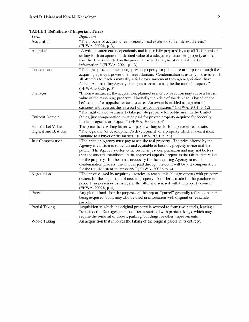
TABLE 1. Definitions of Important Terms Term Definition Acquisition “The process of acquiring real property (real estate) or some interest therein.”

(FHWA, 2002b, p. 3) Appraisal “A written statement independently and impartially prepared by a qualified appraiser

setting forth an opinion of defined value of a adequately described property as of a specific date, supported by the presentation and analysis of relevant market information.” (FHWA, 2001, p. 13)

Condemnation

“The legal process of acquiring private property for public use or purpose through the acquiring agency’s power of eminent domain. Condemnation is usually not used until all attempts to reach a mutually satisfactory agreement through negotiations have failed. An acquiring Agency then goes to court to acquire the needed property.” (FHWA, 2002b, p. 3)

Damages “In some instances, the acquisition, planned use, or construction may cause a loss in value of the remaining property. Normally the value of the damage is based on the before and after appraisal or cost to cure. An owner is entitled to payment of damages and receives this as a part of just compensation.” (FHWA, 2001, p. 52)

Eminent Domain

“The right of a government to take private property for public use. In the United States, just compensation must be paid for private property acquired for federally funded programs or projects.” (FHWA, 2002b, p. 3)

Fair Market Value The price that a willing buyer will pay a willing seller for a piece of real estate. Highest and Best Use “The legal use (or development/redevelopment) of a property which makes it most

valuable to a buyer or the market.” (FHWA, 2001, p. 53) Just Compensation

“The price an Agency must pay to acquire real property. The price offered by the Agency is considered to be fair and equitable to both the property owner and the public. The Agency’s offer to the owner is just compensation and may not be less than the amount established in the approved appraisal report as the fair market value for the property. If it becomes necessary for the acquiring Agency to use the condemnation process, the amount paid through the court will be just compensation for the acquisition of the property.” (FHWA, 2002b, p. 4)

Negotiation

“The process used by acquiring agencies to reach amicable agreements with property owners for the acquisition of needed property. An offer is made for the purchase of property in person or by mail, and the offer is discussed with the property owner.” (FHWA, 2002b, p. 4)

Parcel

Any plot of land. For the purposes of this report, “parcel” generally refers to the part being acquired, but it may also be used in association with original or remainder parcels.

Partial Taking

Acquisition in which the original property is severed to form two parcels, leaving a “remainder”. Damages are most often associated with partial takings, which may require the removal of access, parking, buildings, or other improvements.

Whole Taking An acquisition that involves the taking of the original parcel in its entirety.

Jared D. Heiner and Kara M. Kockelman 13

TABLE 2. Description of Variables for Texas Corridor Data Set Description of Variables for Texas Corridor Sample

Variable Name Variable Description Mean S.D. TOTCOST Total acquisition cost ($2003) 245300 894400 LNTOTCOST Natural log of total cost 10.36 2.091 ACQSF Land area of part acquired (SF) 12120 23850 FRONTAGE Length of frontage (feet) 211.1 314.9 DRIVEWYS Number of driveways for original parcel 1.323 0.600 SHAPEIRR Indicator variable for irregularly shaped

original parcel 0.2491 0.4333 CORNER Indicator variable for corner parcels 0.3614 0.4813 TIME TREND Trend variable for year of acquisition

(1=1997, 2=1998,…7=2003) 4.393 1.517 IMPSF Area of improvements taken (SF) 1545 6276 IMPAGE Age of improvements taken (years) 35.746 21.226 IMPCOND Appraised condition of improvements

(1=Poor, 2=Fair, 3=Average, 4=Good) 3.136 0.846 IMPSF2 Area of improvement squared (SF2) 41640000 448300000 REMSF Remainder area (SF) 188200 745600 CHGHBUSE Indicator variable for a reduction in

highest and best use 0.116 0.321 FRNTLOSS Loss in frontage (feet) 53.70 159.0 RATIO Ratio of remainder area to original area 0.5390 0.4264 SHAPECHG Indicator variable for an acquisition which

effected a change in parcel shape 0.1159 0.3209 PARTIALTKG Indicator variable for partial takings 0.8070 0.3953 VACANT Indicator variable for vacant land 0.1263 0.3328 AGRI Indicator variable for agricultural land 0.0772 0.2674 SFAM Indicator variable for single-family

residential 0.5018 0.5009 MFAM Indicator variable for multi-family

dwellings 0.0351 0.1843 RETAIL Indicator variable for retail uses

(e.g., shopping & restaurants) 0.1754 0.3810 SERVICE Indicator variable for auto repair and

service 0.0456 0.2090 OTHER Indicator variable for other uses

(e.g. churches, medical and dental offices) 0.0351 0.1843 ABILENE Indicator variable for Abilene 0.0561 0.2306 CORPUS Indicator variable for Corpus Christi 0.2000 0.4007 ELPASO Indicator variable for El Paso 0.3193 0.4670 FTWORTH Indicator variable for Fort Worth 0.1439 0.3516 HOUSTON Indicator variable for Houston 0.1754 0.3810 SANANTONIO Indicator variable for San Antonio 0.1053 0.3074

Jared D. Heiner and Kara M. Kockelman 14

TABLE 3. Total Taking-Cost Model Results, using Texas Corridor Data Log-Log Regression Results for Texas Corridor Sample

Dependent Variable: Natural Log of Total Cost Number of Observations 285 Adjusted R-squared 0.906

Variables Coefficient Std. Coef. p-value (Constant) 2.73786 0.000 LN(ACQSF) - - -

LN(ACQSF*CORNER) 0.02105 0.0422 0.047 LN(ACQSF*TIMETREND) 0.49643 0.3612 0.000 LN(ACQSF*VACANT) 0 n/a n/a LN(ACQSF*AGRI) -0.04532 -0.0536 0.081 LN(ACQSF*SFAM) 0.08536 0.1765 0.000 LN(ACQSF*MFAM) 0.07404 0.0538 0.020 LN(ACQSF*RETAIL) 0.13481 0.2176 0.000 LN(ACQSF*SERVICE) 0.07239 0.0556 0.096 LN(ACQSF*OTHER) 0.07900 0.0609 0.011 LN(ACQSF*CORPUS) 0 n/a n/a LN(ACQSF*ELPASO) 0.24731 0.4545 0.000 LN(ACQSF*FTWORTH) 0.12397 0.1731 0.000 LN(ACQSF*HOUSTON) 0.33290 0.5822 0.000 LN(ACQSF*SAN ANTONIO) 0.40861 0.5443 0.000

LN(IMPSF) 0.72522 1.3190 0.003 LN(IMPSF*TIMETREND) -0.38778 -0.8360 0.020 LN(IMPSF*SFAM) 0 n/a n/a LN(IMPSF*RETAIL) -0.06910 -0.0716 0.038 LN(IMPSF*SERVICE) 0.05461 0.0328 0.324 LN(IMPSF*POPDENSITY) -0.10035 -0.3606 0.094

LN(REMSF) 0.03095 0.0769 0.040 LN(REMSF*CHGHBUSE) -0.04654 -0.0689 0.005 LN(REMSF*SHAPECHG) -0.01723 -0.0232 0.258 LN(REMSF*FRNTLOSS) -0.01251 -0.0320 0.145

Jared D. Heiner and Kara M. Kockelman 15

TABLE 4. Description of Variables for TCAD Commercial Sales Data Variable Description Mean S.D. SALEPRICE Sale or list price in U.S. $2003 1861000 137200 LANDSF Land area (SF) 2407000 1050000 IMPSF Improvement area (SF) 21390 1304 IMPSF2 Improvement area squared (SF2) 2.762E+09 1.460E+10 IMPAGE Age of improvement in years 18.45 0.3827

IMPCOND Improvement condition (1=poor, 2=fair, 3=avg, 4=good, 5=excellent)

1.855 1.735

LISTPRICE Indicator variable for list, or asking price 0.2171 0.4124

TIMETREND Time trend variable for year of acquisition (1=2001, 2-2002, and 3=2003) 1.852 0.8033

Land Use Indicators

APARTMNT Indicator variable for apartment 0.1654 0.0101 HIRISE Indicator variable for hi-rise condominium 0.1750 0.0103 LGOFFICE Indicator variable for office larger than 35,000 SF 0.0458 0.2092 MDOFFICE Indicator variable for medium office (10-35K SF) 0.0318 0.0048 SMOFFICE Indicator variable for small office less than 10,000 SF 0.1596 0.3664

MDSTORE Indicator variable for shopping center, grocery or discount store 0.0273 0.0044

SMSTORE Indicator variable for small store or strip center less than 10,000 SF 0.0517 0.0060

RESTRNT Indicator variable for restaurant, night club, fast food 0.0391 0.0053

CONVSTORE Indicator variable for convenience store, gas station, auto repair and service 0.0480 0.0058

SMWAREHS Indicator variable for warehouse less than 20,000 SF 0.0702 0.0069

LGWAREHS Indicator variable for bulk warehouse, flex space, research and development, and manufacturing 0.1115 0.0086

HOTEL Indicator variable for hotel or motel 0.0096 0.0027 RESTHOME Indicator variable for rest home or treatment center 0.0126 0.0030

Area Indicators NWAREA Indicator variable for northwest Travis County 0.0650 0.2466 SWAREA Indicator variable for southwest Travis County 0.1137 0.3176 NEAREA Indicator variable for northeast Travis County 0.2696 0.4439 SEAREA Indicator variable for southeast Travis County 0.5170 0.4999 RRAREA Indicator variable for Round Rock (north Travis Cnty) 0.0310 0.1734

Jared D. Heiner and Kara M. Kockelman 16

TABLE 5. Sales Price Model Results, using TCAD Commercial Sales Data FGLS Regression Results for TCAD Commercial Sales

Dependent Variable: SALEPRICE Number of Observations 1353 Adjusted R-squared 0.858 Variables Coefficient Std. Coef. p-value (Constant) 126169 0.002 LANDSF -0.0004678 -0.0517 0.009

LANDSF*NWAREA 0 n/a n/a LANDSF*SEAREA 14.5324 0.2927 0.000 LANDSF*SWAREA 2.635 0.0187 0.077

IMPSF 70.29 0.5327 0.000 IMPSF*CONDITION 7.292 0.0505 0.011 IMPSF*LISTPRICE 17.67 0.0227 0.084 IMPSF*TIMETREND 12.13 0.1045 0.025 IMPSF*APARTMT 0 n/a n/a IMPSF*HIRISE 113.9 0.0433 0.000 IMPSF*LGOFFICE 43.13 0.3216 0.001 IMPSF*SMWAREHS -28.39 -0.0221 0.048 IMPSF*LGWAREHS -103.9738 -0.1054 0.000 IMPSF*NWAREA 0 n/a n/a IMPSF*NEAREA -24.71 -0.0597 0.052 IMPSF*SEAREA -65.78 -0.1200 0.000

IMPSF2 IMPSF2*APARTMT 0 n/a n/a IMPSF2*CONVSTORE -0.01130 -0.0189 0.069 IMPSF2*LGWAREHS 0.002393 0.0390 0.093 IMPSF2*HOTEL 0.0002403 0.0270 0.014

Jared D. Heiner and Kara M. Kockelman 17

TABLE 6. Description of Variables for CoStar Commercial Sales Data Variables Description Mean SD SALEPRICE Sale or list price in U.S. $2003 2917000 9795000 LOGPRICE Natural log of sales price 13.79 1.317 LANDSF Land area (SF) 672200 6777000 FRONTAGE Length of street frontage in feet 282.5 466.3 CORNER Indicator variable for corner parcel 0.2898 0.4537 IMPSF Improvement area (SF) 37520 103200 IMPAGE Age of Improvement in years 14.27 18.04 IMPCOND Improvement condition (1=poor,

2=fair, 3=avg, 4=good, 5=excellent). 1.847 1.684

TIMETREND Time Trend for year of sale (0 for 1996, 1 for 1997… 7 for 2003).

4.454 1.316

UNCONFIRMED Indicator variable for unconfirmed sales price 0.0345 0.1825

PRKOPEN Number of open-air parking spaces 11.65 137.8 PRKCOVER Number of covered parking spaces 53.89 177.8 APTMT Indicator variable for apartment use 0.1124 0.3159 COMRCL Indicator variable for commercial

land 0.2476 0.4317 HOTEL Indicator variable for hotel or motel 0.0089 0.0940 INDSTRL Indicator variable for industrial use 0.2015 0.4011 MOBILE Indicator variable for mobile home

park 0.0023 0.0476 OFFICE Indicator variable for office use 0.1220 0.3272 RESID Indicator variable for residential land 0.1032 0.3042 RETAIL Indicator variable for retail use 0.1811 0.3851 SPECIAL Indicator variable for special use

(e.g. church, hospital, or school) 0.0210 0.1435

BEXAR Bexar County (San Antonio) 0.0499 0.2177 COLLIN Collin County (Dallas-Fort Worth) 0.0710 0.2568 DALLAS Dallas County (Dallas-Fort Worth) 0.2101 0.4074 DENTON Denton County (Dallas-Fort Worth) 0.0478 0.2133 FORTBEND Fort Bend County (Houston) 0.0290 0.1679 HARRIS Harris County (Houston) 0.2307 0.4213 MONTGMRY Montgomery County (Houston) 0.0190 0.1366 TARRANT Denton County (Dallas-Fort Worth) 0.1393 0.3463 TRAVIS Travis County (Austin) 0.1487 0.3558 WILLIAMSON Williamson County (Austin) 0.0544 0.2269

Jared D. Heiner and Kara M. Kockelman 18

TABLE 7. Sales Price Model Results, using CoStar Commercial Sales Data FGLS Regression Results for CoStar Commercial Sales

Dependent Variable: SALEPRICE Number of Observations 10987 Adjusted R-squared 0.644 Variables Coefficient Std. Coef. p-value (Constant) 538440 0.000 LANDSF 0.5541 0.4408 0.000

LANDSF*FRONTAGE -0.00004411 -0.0544 0.000 LANDSF*APTMT 0 n/a n/a LANDSF*COMRCL 0.1482 0.0801 0.000 LANDSF*HOTEL -12.21 -0.0320 0.015 LANDSF*INDUSTRIAL 0.2556 0.0223 0.003 LANDSF*MOBILE 1.0782 0.0353 0.000 LANDSF*RETAIL 5.625 0.1068 0.000 LANDSF*SPECIAL -1.7000 -0.0344 0.000 LANDSF*BEXAR -0.3483 -0.0329 0.000 LANDSF*COLLIN 0.6327 0.0626 0.000 LANDSF*DALLAS 0 n/a n/a LANDSF*DENTON 0.7403 0.0514 0.000 LANDSF*FORTBEND -0.3440 -0.0784 0.000 LANDSF*MONTGMRY -0.5359 -0.1587 0.000 LANDSF*TRAVIS -0.2555 -0.0613 0.000 LANDSF*WILLIAMSN -0.5083 -0.3099 0.000

IMPSF 21.16 0.2810 0.000 IMPSF*IMPAGE -0.6854 -0.2667 0.000 IMPSF*IMPCOND 9.228 0.3986 0.000 IMPSF*NUMFLOORS 2.079 0.1232 0.000 IMPSF*HOTEL 39.09 0.0481 0.000 IMPSF*APTMT 0 n/a n/a IMPSF*INDSTRL -13.85 -0.1120 0.000 IMPSF*OFFICE 14.97 0.0704 0.000 IMPSF*RETAIL -13.89 -0.0627 0.000 IMPSF*SPECIAL 36.62 0.0773 0.000 IMPSF*BEXAR -8.839 -0.0173 0.017 IMPSF*COLLIN 15.35 0.0388 0.000 IMPSF*FORT BEND 9.308 0.0186 0.011 IMPSF*DALLAS 0 n/a n/a IMPSF*HARRIS -4.932 -0.0364 0.000 IMPSF*TARRANT -5.274 -0.0286 0.000 IMPSF*TRAVIS 16.12 0.0550 0.000 IMPSF*WILLIAMSON 14.49 0.0245 0.001

PRKCOVER 6026 0.0771 0.000 UNCONFIRMED 206405 0.0162 0.022

Jared D. Heiner and Kara M. Kockelman 19

APPENDIX

TABLE A1. Variance Model Results, using TCAD Commercial Sales Data

Variance Model for TCAD Commercial Sales Dependent Variable: Squared Residuals Number of Observations 1353 Adjusted R-squared 0.455 Variables Coefficient Std. Coef. p-value (Constant) 23.63 0.000 LANDSF -1.119E-08 -0.1396 0.000

LANDSF*LISTPRICE -5.520E-09 -0.0456 0.147 LANDSF*NWAREA 0 n/a n/a LANDSF*NEAREA 9.865E-09 0.1055 0.022 LANDSF*SEAREA 5.187E-07 0.0978 0.000 LANDSF*RRAREA -2.425E-06 -0.0354 0.115

IMPSF 5.440E-05 0.8427 0.000 IMPSF*IMPAGE 1.756E-07 0.0399 0.163 IMPSF*IMPCOND 5.530E-06 0.1209 0.004 IMPSF*TIMETREND 6.627E-06 0.1840 0.000 IMPSF*APARTMT 0 n/a n/a IMPSF*HIRISE -8.021E-04 -0.1372 0.000 IMPSF*LGOFFICE -7.079E-06 -0.0773 0.268 IMPSF*MDOFFICE 4.728E-05 0.0649 0.002 IMPSF*SMOFFICE -2.776E-04 -0.1587 0.028 IMPSF*MDSTORE 8.390E-05 0.1854 0.001 IMPSF*RESTRNT 4.592E-04 0.1568 0.006 IMPSF*CONVSTORE -2.128E-04 -0.0673 0.110 IMPSF*SMWAREHS 2.125E-05 0.1201 0.000 IMPSF*LGWAREHS -8.326E-05 -0.0932 0.035 IMPSF*HOTEL 1.953E-05 0.0691 0.238 IMPSF*NWAREA 0 n/a n/a IMPSF*SEAREA -9.821E-06 -0.1060 0.001

IMPSF2 -1.636E-10 -0.7703 0.000 IMPSF2*APARTMT 0 n/a n/a IMPSF2*HIRISE -2.717E-08 -0.0297 0.164 IMPSF2*LGOFFICE 1.005E-10 0.3443 0.000 IMPSF2*SMOFFICE 4.241E-08 0.1882 0.543 IMPSF2*MDSTORE -8.242E-10 -0.1286 0.986 IMPSF2*RESTRNT -3.241E-08 -0.0931 0.100 IMPSF2*CONVSTOR 2.107E-08 0.0871 0.036 IMPSF2*LGWAREHS 2.265E-09 0.0578 0.180 IMPSF2*HOTEL -1.121E-10 -0.1055 0.050

Jared D. Heiner and Kara M. Kockelman 20

TABLE A2. Variance Model Results, using CoStar Commercial Sales Data Variance Model Results for CoStar Commercial Sales

Dependent Variable: Natural Log of Squared OLS Residuals Number of Observations 10987 Adjusted R-squared 0.259 Variables Coefficient Std. Coef. p-value (Constant) 25.28 0.000 LANDSF 3.349E-07 0.7539 0.000

LANDSF*FRONTAGE -1.215E-11 -0.0445 0.009 LANDSF*HOTEL 4.906E-06 0.0207 0.083 LANDSF*INDUSTRIAL 3.467E-07 0.0432 0.000 LANDSF*RETAIL 2.655E-06 0.1250 0.000 LANDSF*SPECIAL 6.010E-07 0.0305 0.000 LANDSF*BEXAR -1.315E-07 -0.0257 0.018 LANDSF*COLLIN 2.089E-07 0.0433 0.000 LANDSF*DENTON 3.153E-07 0.0404 0.000 LANDSF*FORTBEND -2.544E-07 -0.0877 0.000 LANDSF*HARRIS -1.344E-07 -0.0427 0.007 LANDSF*MONTGMRY -2.678E-07 -0.0878 0.000 LANDSF*TARRANT -1.836E-07 -0.0535 0.000 LANDSF*TRAVIS -2.259E-07 -0.0956 0.000 LANDSF*WILLIAMSN -3.112E-07 -0.6509 0.000

IMPSF 8.781E-06 0.3012 0.000 IMPSF*IMPCOND 5.331E-07 0.0671 0.018 IMPSF*NUMFLOORS -2.034E-07 -0.0927 0.000 IMPSF*HOTEL 8.383E-06 0.0243 0.042 IMPSF*INDSTRL -1.433E-06 -0.0224 0.033 IMPSF*OFFICE 7.390E-06 0.1286 0.000 IMPSF*RETAIL -4.418E-06 -0.0619 0.000 IMPSF*BEXAR 6.172E-06 0.0224 0.008 IMPSF*DENTON -1.819E-06 -0.0395 0.008 IMPSF*HARRIS 1.776E-06 0.0394 0.012 IMPSF*MONTGMRY 7.459E-06 0.0222 0.008 IMPSF*TRAVIS 3.448E-06 0.0295 0.002

PRKCOVER -8.705E-04 -0.0398 0.004 PRKOPEN 2.038E-03 0.1204 0.000 UNCONFIRMED SALE 5.998E-01 0.0364 0.000

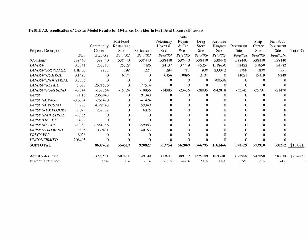
TABLE A3. Application of CoStar Model Results for 10-Parcel Corridor in Fort Bend County (Houston)

Property Description Community

Center

Fast Food Restaurant

Site Restaurant

Veterinary Hospital

Site

Auto Repair & Car Wash

Drug Store Site

Airplane Hangars

Site Restaurant

Site

Strip Center

Site

Fast Food Restaurant

Site Total Co Beta Beta*X1 Beta*X2 Beta*X3 Beta*X4 Beta*X5 Beta*X6 Beta*X7 Beta*X8 Beta*X9 Beta*X10 (Constant) 538440 538440 538440 538440 538440 538440 538440 538440 538440 538440 538440 LANDSF 0.5541 253313 25328 17486 24137 37749 45254 1518650 52422 57650 34582 LANDSF*FRONTAGE 4.4E-05 -8822 -298 -224 -294 -781 -908 -233342 -1799 -1808 -551 LANDSF*COMRCL 0.1482 0 6774 0 6456 10096 12104 0 14021 15419 9249 LANDSF*INDUSTRIAL 0.2556 0 0 0 0 0 0 700536 0 0 0 LANDSF*RETAIL 5.625 2571536 0 177514 0 0 0 0 0 0 0 LANDSF*FORTBEND -0.344 -157264 -15724 -10856 -14985 -23436 -28095 -942818 -32545 -35791 -21470 IMPSF 21.16 2363043 0 91348 0 0 0 0 0 0 0 IMPSF*IMPAGE -0.6854 -765420 0 -41424 0 0 0 0 0 0 0 IMPSF*IMPCOND 9.228 4122148 0 159349 0 0 0 0 0 0 0 IMPSF*NUMFLOORS 2.079 232172 0 8975 0 0 0 0 0 0 0 IMPSF*INDUSTRIAL -13.85 0 0 0 0 0 0 0 0 0 0 IMPSF*OFFICE 14.97 0 0 0 0 0 0 0 0 0 0 IMPSF*RETAIL -13.89 -1551166 0 -59963 0 0 0 0 0 0 0 IMPSF*FORTBEND 9.308 1039471 0 40183 0 0 0 0 0 0 0 PRKCOVER 6026 0 0 0 0 0 0 0 0 0 0 UNCONFIRMED 206405 0 0 0 0 0 0 0 0 0 0 SUBTOTAL 8637452 554519 920827 553754 562069 566795 1581466 570539 573910 560252 $15,081,5

Actual Sales Price 13227581 602411 1149199 313601 389722 1229199 1830686 682988 542050 516038 $20,483,4Percent Difference 35% 8% 20% -77% -44% 54% 14% 16% -6% -9% 2