The Cost of Uncertainty about the Timing of

Social Security Reform∗

Frank N. Caliendo† Aspen Gorry‡ Sita Slavov§

This Version: May 14, 2015. First Version: November 5, 2013.

Abstract

We develop a methodology to study how uncertainty about the timing of the resolu-

tion of uncertainty affects economic decision making and welfare. As an example of the

power of our framework, we analytically solve and simulate household decisions and welfare

in a setting in which households don’t know how or when Social Security is going to be

reformed. Uncertainty about the structure and timing of Social Security reform is regres-

sive: the very low income group from the 2013 Trustees Report (who earn 25 percent of the

economy-wide average wage) experience a welfare loss that is about 3 times larger than those

who earn the maximum taxable amount in each year of their career.

∗We thank Shantanu Bagchi, Peter Bossaerts, Eric Fisher, Jim Feigenbaum, Carlos Garriga, Nick Guo, Tim

Kehoe, Sagiri Kitao, Jorge Alonso Ortiz, Kerk Phillips, Jennifer Ward-Batts, Jackie Zhou, and seminar audiences

at ITAM, UConn, Midwest Macro at Minnesota, Utah State University, BYU-USU Macro Workshop, University

of Nevada Reno, CUNY Hunter College, and the 2014 WEAI conference for helpful comments and suggestions.†Utah State University. Email: frank.caliendo@usu.edu.‡Utah State University. Email: aspen.gorry@usu.edu.§George Mason University. Email: sslavov@gmu.edu.

1

1. Introduction

How does uncertainty about the timing of the resolution of uncertainty affect economic decision

making and welfare? Some researchers have considered the implications of uncertainty that is

resolved at different time horizons, but the timing of the resolution of uncertainty is typically known

in advance.1 We are interested in situations in which decision makers not only face uncertainty

about the outcome of a future event (structural uncertainty), but the timing of that event is also

uncertain (timing uncertainty). For example, young Americans who must make consumption and

saving plans for retirement don’t know how or when Social Security will be reformed.

We develop a dynamic setting to study decision making in the face of both structural and

timing uncertainty. Our setting has three main features:

First, with two layers of uncertainty instead of just one, our analysis differs from a related

literature that seeks to understand how the timing of the resolution of uncertainty affects decision

making. Rather than modeling timing uncertainty, this literature focuses on understanding how

early versus late resolution of uncertainty affects decision making. In each case, the timing of the

resolution of uncertainty is known in advance.2

Second, we allow for flexible distributions over the resolution of timing uncertainty. This allows

the framework to handle non-stationary distributions of the timing of events, which contrasts with

the standard stochastic dynamic programming setting in which uncertainty is represented as a

Markov process and hence is stationary, depending only on the state. Our methodology is flexible

1Long-run risk models are an example. Epstein et al. (2014) provide an overview of this literature and they

compute the “timing premium”under recursive preferences, which is the amount households would be willing to pay

to resolve uncertainty about future consumption right away. But there is no timing uncertainty in their setting.

Households always know in advance whether they are living in the early-resolution world or the late-resolution

world, and then the experiment is to calculate how much households in the second world would pay to live in the

first.2Blundell and Stoker (1999) and Eeckhoudt et al. (2005) study the connection between optimal consumption

and the timing of income risk. They compare the case in which income risk gets resolved early to the case in which

income risk gets resolved late, but in each case the household knows when the income risk gets resolved. Likewise,

Wright et al. (2014) extend these ideas to firm investment behavior. They seek to understand the differential effects

of long and short term uncertainty on firm investment policy, but firms in their model don’t face uncertainty about

when this uncertainty gets resolved.

2

enough to handle both the Markovian case in which the distribution over a shock date is time

invariant and the case in which the distribution is a function of the date itself. For instance, it

may be that one can characterize uncertainty about the timing of Social Security reform as a state

dependent process, but it is convenient to specify the distribution of reform dates as a function

of time itself. This allows us to quickly consider a wide variety of distributions without having

to reconsider the appropriate state space.3 We do this by combining and generalizing existing

tools from the two-stage optimal control literature that deal independently with either structural

uncertainty or with timing uncertainty but not both at once.4

Third, our analysis is developed to obtain quantitative answers to important policy questions.

Understanding how to measure policy uncertainty, and how policy uncertainty affects economic

decisions, has become a priority in macroeconomics (Sargent (2005), Baker et al. (2013), Baker

et al. (2014)).5 Our paper provides some of the tools that are needed to evaluate the impact of

policy uncertainty when the underlying uncertainty has both a structural component and a timing

3We are interested in a variety of possible distributions, such as the stationary case with a constant hazard rate

of reform, the non-stationary case with a spike in the likelihood of reform near the date at which the trust fund is

projected to run out of money, and the non-stationary case in which the likelihood of reform increases with each

passing day.4Examples of two-stage control problems with a stochastic regime switch date (timing uncertainty) can be found

in the early studies on resource extraction (Dasgupta and Heal (1974)), operations research (Kamien and Schwartz

(1971)), and environmental catastrophe (Clarke and Reed (1994)). And examples of problems with uncertainty

about the characteristics of the new regime (structural uncertainty) appeared in the early resource extraction

literature (Hoel (1978)) and later in the technology adoption literature (Hugonnier et al. (2006), Pommeret and

Schubert (2009), Abel and Eberly (2012)). Our theoretical contribution is to build a bridge between these literatures

by generalizing these specific examples and summarizing how to nest both layers of uncertainty together in a single

control problem.5Uncertainty about future policy can affect investment, saving, and hiring decisions (Rodrik (1989), Bernanke

(1983)). The impact of policy uncertainty on firms’ decisions and profitability can be substantial, potentially

resulting in large effi ciency costs. Several studies estimate or calibrate models in which taxes, government spending,

or other policies are uncertain, and then explore the economic impacts of this uncertainty (Fernández-Villaverde

et al. (2013), Croce et al. (2012), Hassett and Metcalf (1999), Pastor and Veronesi (2011), Sialm (2006), Ulrich

(2012)). Others use the timing of national elections as a measure of policy uncertainty, examining the impact of

uncertain election outcomes on economic behavior (Belo et al. (2011), Boutchkova et al. (2012), Durnev (2010),

Julio and Yook (2012), Pantzalis et al. (2000)).

3

component.

To show the power of this framework, we tackle the important example of policy induced

uncertainty that we have alluded to already. It is well known that the Social Security Old Age,

Survivors, and Disability Insurance (OASDI) program faces severe long run solvency concerns.

The 2013 Social Security Trustees Report projects that the program’s trust fund will run out of

money in the year 2033.6 This means that over the coming decades either promised retirement

benefits must be cut or the payroll taxes used to fund them must be increased to keep the program

solvent. Gokhale (2013) estimates that an immediate tax increase of 3.1% of taxable wages, or an

immediate benefit cut of 21%, will keep the OASI part of the program (which we focus on in this

paper) solvent for the infinite horizon.7

While there is very little uncertainty about the need for reform, there is a great deal of uncer-

tainty surrounding its timing and structure. For instance, Sargent (2005) states: “We do not know

today...how subsequent political deliberations from shifting majority coalitions will render U.S. fis-

cal policy coherent.”8 And even though the feasibility/optimality of various Social Security reforms

have been widely studied in macroeconomic models (e.g., McGrattan and Prescott (2014) and Ki-

tao (2014) and the references therein), this literature treats the timing and structure of reform

as part of the household information set, which allows researchers to construct general equilibria.

Again, Sargent (2005) states: “The rational expectations equilibrium concept common to all of our

models requires...that an agent living within one of these models would know the monetary and

fiscal policies affecting him.”We focus on the primary question of measuring welfare losses to a

single individual in an environment where the timing and structure of reform are unknown and

general equilibria cannot be computed because fiscal policy is not yet coherent.9

6Throughout the paper we refer to the 2013 Trustees Report because the 2014 Trustees Report doesn’t have

replacement rates for hypothetical earners or the estimated benefit cut required to balance the long-term budget.7If the disability component of the program is also included, then the required tax increase (assuming no

behavioral response) is 4% and the required benefit cut is 23.9% as estimated in the 2013 Trustees Report.8This uncertainty arises not only from the reluctance of elected offi cials to propose unpopular reforms, but also

from ongoing disagreements over which reform option is most desirable. In particular, Democrats have tended to

favor tax increases, while Republicans have tended to favor benefit cuts. For more detail, see recent legislation

introduced by members of Congress and summarized by the Offi ce of the Chief Actuary, at www.ssa.gov.9While Bütler (1999) studies a particular example of the implications of uncertainty about both the timing and

structure of social security reform in Switzerland, our methodology allows us to handle any assumptions about the

4

We use our method to characterize and simulate household consumption/saving decisions and

welfare under uncertainty about the structure and timing of Social Security reform. We parame-

terize the model to match individual wage and survival profiles. The parameterized model allows

us to assess the welfare cost of uncertainty surrounding the timing and structure of Social Security

reform. We measure this cost as the fraction of lifetime consumption that a young individual

facing reform uncertainty over the life cycle would be willing to give up to live in a separate world

with no reform uncertainty and endowed with wealth that is equal to expected wealth over all

possible dates and structures of reform. Endowing the individual in the no-uncertainty world in

this manner acts to net out the cost of reform itself (which we already know is large, e.g., Kitao

(2014)), allowing us to quantify the welfare cost of this specific example of policy induced uncer-

tainty.10 The government can eliminate this cost by simply announcing a date and structure of

reform.

Because Social Security benefits and taxes vary with income, the impact of Social Security

reform uncertainty may vary across income groups. To be more specific, Social Security is financed

by a proportional payroll tax up to a taxable maximum wage ($113,700 in 2013).11 But benefits

are paid according to a progressive formula that gives individuals with low lifetime earnings higher

replacement rates (benefits as a share of average lifetime earnings). Since all individuals face the

distributions of both structural and timing uncertainty. This flexibility allows us to study timing and structural

uncertainty in a general way and to explore the distributional effects of reform in the US.10Bütler (1999) studies the welfare cost of uncertainty about the timing of social security reform in Switzerland.

However, she compares the welfare of individuals who must live with timing uncertainty to individuals who live

in a separate world with no timing uncertainty and with reform that is guaranteed to happen at the date that is

mathematically expected in the first world. While such a comparison would certainly capture important differences

in behavior, it does not actually pin down the cost of uncertainty. Instead, it confounds changes in wealth with

the effects of uncertainty. In fact, with such a comparison it is theoretically possible to come to the mistaken

conclusion that uncertainty actually is a good thing (because it increases an individual’s expected lifetime wealth).

For instance, if we assume that individuals in the first world are uncertain about when a benefit cut will strike and

the mathematical expectation is that it will strike just before retirement, then individuals would want maximum

variance around this expectation in order to create the possibility of collecting full benefits for at least some portion

of the retirement period.11The taxable maximum is $118,500 in 2015, but again we focus on 2013 values throughout the paper because

the 2013 Trustees Report is more comprehensive.

5

same tax rate (at least up through the taxable maximum income), but receive different replacement

rates, we can vary the replacement rate in our model to simulate the effect of Social Security reform

uncertainty for individuals of different incomes.

Uncertainty about the timing of reform is considered first because timing uncertainty is harder

to deal with theoretically and because less is known about its welfare consequences. In this

scenario, the individual has full information about the structure of reform and we consider the

possibility of either a known benefit cut or a known tax increase occurring at an unknown date.

Uncertainty about the timing of reform has moderate costs to individuals of average income,

a result which holds regardless of whether reform takes the form of across-the-board tax increases

or across-the-board benefit cuts. However, tax increases and benefit cuts have different effects for

low-income and high-income individuals. If individuals know that the Social Security budget will

be balanced using an across-the-board benefit cut, uncertainty about the timing of reform harms

low-income individuals more because Social Security accounts for a larger portion of their lifetime

wealth. Alternatively, when the budget will be balanced using an across-the-board tax increase,

high-income individuals earning the taxable maximum face larger welfare losses because they face

the same percentage tax increase but rely less on the progressive benefit.

In addition to timing uncertainty, individuals also do not know the structure of future reform.

The government may balance the budget through tax increases, benefit cuts, or some combination

of the two. After adding this second layer of uncertainty to our model, the overall welfare cost

of the combined reform uncertainty can be greater or less than the cost for the case where there

is only timing uncertainty. However, we find that this double uncertainty consistently imposes

much larger welfare costs on low-income individuals across all parameterizations of the model.

The very low income group from the 2013 Trustees Report (who earn 25 percent of the economy-

wide average wage) experience a welfare loss that is about 3 times larger than those who earn the

maximum taxable amount in each year of their career.

This paper is related to Gomes et al. (2007), Benítez-Silva et al. (2007) and Luttmer and

Samwick (2012) who also quantify the costs of Social Security reform uncertainty. Gomes et al.

(2007) study a model environment in which there is uncertainty about whether a benefit cut will

occur at a given future date. Their baseline household would be willing to give up 0.12% of annual

consumption in exchange for learning about the cut to Social Security benefits at age 35 instead

6

of age 65. While this result has a similar flavor to ours, their model likely overstates the result by

placing the uncertainty at the worst possible date (i.e., at retirement) rather than modeling the

full uncertainty about the timing of reform. Households in their model never actually face timing

uncertainty because the date at which information is released is known in advance.12 ,13

Similar to Gomes et al. (2007), Benítez-Silva et al. (2007) also compute the welfare loss from

having to live with uncertainty about the future level of Social Security benefits. There is no

timing uncertainty in their model either. And Luttmer and Samwick (2012) use survey data to

elicit the degree of Social Security reform uncertainty that individuals perceive, and how costly

such uncertainty is to them. They find that individuals would be willing to tolerate an additional

4-6% cut in benefits in exchange for certainty about their level.

Some studies of fiscal policy uncertainty do consider both timing uncertainty and structural

uncertainty (e.g., Davig and Foerster (2014), Stokey (2014)), but they differ from our study in

two ways. First, they do not focus specifically on Social Security reform. And second, they model

timing uncertainty as a stationary process.

Finally, we depart from a literature that assumes individuals don’t fully understand the rules

of Social Security. In that literature, information is costly to acquire or individuals lack the

ability to process information, while the political process is stationary and the rules are knowable

(Liebman and Luttmer (2014)). In our setting individuals are rational and have full information

about everything that is knowable, which includes the distributions of random variables relating

to political risks, while the realization of these random variables is unknowable. This implies that

our estimates of the cost of uncertainty about Social Security reform are likely a lower bound.

12Gomes et al. (2007) also consider the gains from early resolution of uncertainty about the magnitude of a

future tax increase. But once again households know in advance the future date at which the government will

release the information, so timing uncertainty is absent.13Evans et al. (2012) consider a model in which future transfers to the old are uncertain because transfers are

based on the stochastic wages of the young. If promised transfers are infeasible because of a negative productivity

shock, the government switches to a more affordable transfer scheme. Likewise, van der Wiel (2008) considers the

effect of uncertainty about future Social Security benefits on private savings, but similar to Gomes et al. (2007), the

individual knows in advance that the government will announce the new level of benefits at the date of retirement,

so there is no timing uncertainty.

7

2. Theory: Timing Uncertainty and Structural Uncertainty

In this section we provide a self contained summary of how to solve a generic dynamic problem

that features both timing uncertainty and structural uncertainty. Problem 1 features timing

uncertainty only. And Problem 2 features both timing uncertainty and structural uncertainty.14

Contemporaneously with our study, Stokey (2014) uses the same dynamic optimization methods.

Time is continuous and indexed by t. Time starts at t = 0 and never ends. The planning

interval of the decision maker, which begins at t = 0 and ends at t = T , is comprised of two

regimes or stages. The first stage stretches from t = 0 to t = t1, and the second stage stretches

from t = t1 to t = T . Each stage has a unique performance index and/or a unique state equation.

The regime switch date t1 is a continuous random variable, with probability density φ(t1) and

sample space [0,∞]. The control variable u(t) is unconstrained and the state variable x(t) is

constrained only at the initial and terminal points in time.

Problem 1 (Timing Uncertainty Only).

maxu(t)t∈[0,T ]

: J = E[∫ t1

0

f1(t, u(t), x(t))dt+

∫ T

t1

f2(t, u(t), x(t))dt

], (1)

subject todx(t)

dt= g1(t, u(t), x(t)), for t ∈ [0, t1], (2)

dx(t)

dt= g2(t, u(t), x(t)), for t ∈ [t1, T ], (3)

x(0) = x0, x(T ) = xT , (4)

t1 random with density φ(t1) and sample space [0,∞]. (5)

14Our analysis builds on the two-stage control literature in which the switch date is deterministic and may be

a choice variable or exogenous (Kemp and Long (1977), Tomiyama (1985), Amit (1986), Tahvonen and Withagen

(1996), Makris (2001), Boucekkine et al. (2004), Dogan et al. (2011), Saglam (2011), Boucekkine et al. (2012),

Boucekkine et al. (2013a), and Boucekkine et al. (2013b)).

8

It is helpful to lay out some assumptions and definitions before stating the necessary conditions.

Assumption 1 (Differentiability). The functions f1, f2, g1, g2, and φ(t1) are continuously

differentiable in their arguments.

Definition 1 (Solution Notation). Let (u∗2(t|t1, x(t1)), x∗2(t|t1, x(t1)))t∈[t1,T ] be the optimal

control and state path for any t after the realization of the random regime switch, conditional on

the switch date t1 and conditional on the stock of the state variable at that switch date x(t1).

Similarly, let (u∗1(t), x∗1(t))t∈[0,T ] be the optimal control and state path for any t before the

realization of the random switch. Hence, the path that is actually followed, conditional on switch

date t1, is (u∗1(t), x∗1(t))t∈[0,t1] and (u∗2(t|t1, x∗1(t1)), x∗2(t|t1, x∗1(t1)))t∈[t1,T ].

Theorem 1 (Necessary Conditions to Problem 1). The necessary conditions can be

derived recursively in two steps.15

Step 1. Solve the post-switch (t = t1) subproblem:

The program (u∗2(t|t1, x(t1)), x∗2(t|t1, x(t1)))t∈[t1,T ] solves a fixed endpoint Pontryagin subproblem

maxu(t)t∈[t1,T ]

: J2 =

∫ T

t1

f2(t, u(t), x(t))dt, (6)

subject todx(t)

dt= g2(t, u(t), x(t)), for t ∈ [t1, T ], (7)

t1 given, x(t1) given, x(T ) = xT . (8)

Given the Hamiltonian function

H2 = f2(t, u(t), x(t)) + λ2(t)g2(t, u(t), x(t)), (9)

15We refer readers to Appendix A for a full derivation of the theorem.

9

the necessary conditions that must hold on the path (u∗2(t|t1, x(t1)), x∗2(t|t1, x(t1)))t∈[t1,T ] include

∂H2/∂u(t) = 0 and dλ2(t)/dt = −∂H2/∂x(t). For convenience, change the time dummy t to z,

and change the switch point t1 to t and write the solution (u∗2(z|t, x(t)), x∗2(z|t, x(t)))z∈[t,T ]. Thus

we have the optimal control and state paths for all points in time z greater than switch point t.

Step 2. Solve the pre-switch (t = 0) subproblem:

The program (u∗1(t), x∗1(t))t∈[0,T ] solves a fixed endpoint Pontryagin subproblem with continuation

function S(t, x(t)):

maxu(t)t∈[0,T ]

: J1 =

∫ T

0

{[∫ ∞t

φ(t1)dt1

]f1(t, u(t), x(t)) + φ(t)S(t, x(t))

}dt, (10)

subject to

S(t, x(t)) =

∫ T

t

f2(z, u∗2(z|t, x(t)), x∗2(z|t, x(t)))dz, (11)

dx(t)

dt= g1(t, u(t), x(t)), for t ∈ [0, T ], (12)

x(0) = x0, x(T ) = xT . (13)

Given the Hamiltonian function

H1 =

[∫ ∞t

φ(t1)dt1

]f1(t, u(t), x(t)) + φ(t)S(t, x(t)) + λ1(t)g1(t, u(t), x(t)), (14)

the necessary conditions that must hold on the path (u∗1(t), x∗1(t))t∈[0,T ] include ∂H1/∂u(t) = 0

and dλ1(t)/dt = −∂H1/∂x(t).

Corollary 1 (Suffi ciency). If g1 and g2 are linear in u(t) and x(t) and the integrands of J1 and

J2 are concave in u(t) and x(t), then the necessary conditions are suffi cient (Mangasarian (1966)).

Checking the concavity of the integrand of J2 is standard. But checking the concavity of the

integrand of J1 is more involved. This is because the integrand of J1 depends on the optimal post-

switch path. Thus, one must first derive the post-switch solution (u∗2(z|t, x(t)), x∗2(z|t, x(t)))z∈[t,T ],

10

which depends on x(t), and then insert this solution into S before checking the concavity of the

integrand of J1.

Finally, to conclude this section we note that in addition to stochastic timing of the regime

switch, we can easily allow for the possibility that the structure of the new regime itself (the

functional form of the post-switch state equation) is uncertain. Adding in this second layer of

uncertainty is relatively easy and requires just a few adjustments to Problem 1 and Theorem 1.16

Problem 2 (Timing Uncertainty and Structural Uncertainty). Add the following to

Problem 1: the uncertainty about the functional form of g2 is summarized by the random

variable α, with density θ(α) and sample space normalized to [0, 1], where θ(α) is continuously

differentiable and realizations of α and t1 are uncorrelated.

Theorem 2 (Necessary Conditions to Problem 2). Follow Theorem 1 to recursively derive

necessary conditions with the following slight modifications: in Step 1 use the notation

g2(t, u(t), x(t)|α) and (u∗2(t|t1, x(t1), α), x∗2(t|t1, x(t1), α))t∈[t1,T ] to emphasize dependence of the

solution on the realization of α, and in Step 2 write the continuation function S(t, x(t), α) and

replace the last term in the integrand of J1 with∫ 10θ(α)φ(t)S(t, x(t), α)dα.

16Models with uncertainty about the structure of the new regime appeared in the early resource extraction

literature (Hoel (1978)) and then again in the more modern literature on technology adoption when future returns

to technology are stochastic (Hugonnier et al. (2006), Pommeret and Schubert (2009), Abel and Eberly (2012)).

Problem 2 and Theorem 2 show how to augment our previous control problem to include both layers of uncertainty.

11

3. Application 1: Uncertainty about the Timing of Reform

We begin with an application of Problem 1. We first introduce notation, then we present the

household optimization problem and welfare, and finally we parameterize the model and simulate

quantitative results.

3.1. Notation

Age is continuous and is indexed by t. Households are born at t = 0 and pass away no later than

t = T . The probability of surviving to age t is Ψ(t). Retirement and benefit collection occur

exogenously at t = tR and labor is supplied inelastically.17 A given household collects wages at

rate w(t) during the working period.

The government’s current policy is summarized by a tax rate on wage earnings and benefit

annuity (τ 1, b1). The current policy is unsustainable and this is publicly known. Therefore house-

holds know that reform is coming, but they don’t know when. The reform date t1 is a random

variable with probability density φ(t1) and sample space [0,∞].

The post-reform policy is (τ 2, b2). For now, we assume households have full information about

the nature of the reform (τ 2, b2), they just don’t know when it will kick in. Thus we are dealing

with an application of Problem 1 from the previous section and Theorem 1 applies.

To compress notation let y1(t) be disposable income before the reform and let y2(t) be dispos-

able income after the reform,

y1(t) =

(1− τ 1)w(t), for t ∈ [0, tR],

b1, for t ∈ [tR, T ],(15)

y2(t) =

(1− τ 2)w(t), for t ∈ [0, tR],

b2, for t ∈ [tR, T ].(16)

Consumption is c(t) and savings is k(t), which earns interest at rate r.

17People predominantly retire from the labor force at the early and normal eligibility ages (see Diamond and

Gruber (1999) among others). Fixing the retirement and collection dates allows us to parameterize the model to

empirically reasonable values for these choices while abstracting from natural and institutional complications that

shape the incentives behind these choices.

12

3.2. Household Problem

Period utility is CRRA with relative risk aversion σ, and utils are discounted at the rate of time

preference ρ. The household solves a dynamic stochastic control problem, taking as given the

disposable income functions y1(t) and y2(t) while treating the reform date t1 as a random variable:

maxc(t)t∈[0,T ]

: J = E[∫ T

0

e−ρtΨ(t)c(t)1−σ

1− σ dt

], (17)

subject todk(t)

dt= rk(t) + y1(t)− c(t), for t ∈ [0, t1], (18)

dk(t)

dt= rk(t) + y2(t)− c(t), for t ∈ [t1, T ], (19)

k(0) = 0, k(T ) = 0, (20)

t1 random with density φ(t1) and sample space [0,∞]. (21)

We refer readers to Appendix B for a step-by-step derivation of the solution to this problem.

In brief, using Theorem 1 as our guide, we solve this problem recursively: following Step 1 we find

that the post-reform (after the shock has hit) consumption path is

c∗2(t|t1, k(t1)) =k(t1) +

∫ Tt1e−r(v−t1)y2(v)dv∫ T

t1e−r(v−t1)+(r−ρ)v/σΨ(v)1/σdv

e(r−ρ)t/σΨ(t)1/σ, for t ∈ [t1, T ]. (22)

Note that consumption after reform depends on the timing of reform and on the stock of assets at

the time of reform. Then, following Step 2, using the post-reform solution, and working backwards,

we find that the pre-reform solution (c∗1(t), k∗1(t))t∈[0,T ] solves the following system of differential

equations and boundary conditions18

dc(t)

dt=

(c(t)σ+1

Ψ(t)

[k(t) +

∫ Tte−r(v−t)y2(v)dv∫ T

te−r(v−t)+(r−ρ)v/σΨ(v)1/σdv

]−σe(ρ−r)t − c(t)

)×[σ

φ(t)

∫ ∞t

φ(t1)dt1

]−1+

[dΨ(t)

dt

1

Ψ(t)+ r − ρ

]c(t)

σ, (23)

18This system must be solved numerically. We guess and interate on c(0) until all the constraints are satisfied.

13

dk(t)

dt= rk(t) + y1(t)− c(t), (24)

k(0) = 0, k(T ) = 0. (25)

Finally, with the stage-one solution (c∗1(t), k∗1(t))t∈[0,T ], we can obtain the explicit stage-two

solution conditional on realization of reform date t1,

c∗2(t|t1, k∗1(t1)) =k∗1(t1) +

∫ Tt1e−r(v−t1)y2(v)dv∫ T

t1e−r(v−t1)+(r−ρ)v/σΨ(v)1/σdv

e(r−ρ)t/σΨ(t)1/σ, for t ∈ [t1, T ]. (26)

3.3. Welfare

As a point of reference, consider the case where the individual faces no risk (NR) about future

taxes and benefits. The individual is endowed at t = 0 with expected future income and solves

maxc(t)t∈[0,T ]

:

∫ T

0

e−ρtΨ(t)c(t)1−σ

1− σ dt, (27)

subject todk(t)

dt= rk(t)− c(t), (28)

k(0) =

∫ T

0

φ(t1)Y (t1)dt1 +

[∫ ∞T

φ(t1)dt1

] ∫ T

0

e−rvy1(v)dv, k(T ) = 0, (29)

where

Y (t1) ≡∫ t1

0

e−rvy1(v)dv +

∫ T

t1

e−rvy2(v)dv. (30)

The solution is

cNR(t) =

∫ T0φ(t1)Y (t1)dt1 +

[∫∞Tφ(t1)dt1

] ∫ T0e−rvy1(v)dv∫ T

0e−rv+(r−ρ)v/σΨ(v)1/σdv

e(r−ρ)t/σΨ(t)1/σ, for t ∈ [0, T ]. (31)

14

The welfare cost of living with reform uncertainty ∆ is the solution to the following equation

∫ T

0

e−ρtΨ(t)[cNR(t)(1−∆)]1−σ

1− σ dt (32)

=

∫ T

0

φ(t1)

(∫ t1

0

e−ρtΨ(t)c∗1(t)

1−σ

1− σ dt+

∫ T

t1

e−ρtΨ(t)c∗2(t|t1, k∗1(t1))1−σ

1− σ dt

)dt1

+

[∫ ∞T

φ(t1)dt1

] ∫ T

0

e−ρtΨ(t)c∗1(t)

1−σ

1− σ dt.

Notice that ∆ captures just the cost of uncertainty about reform, and not the cost of reform

itself. It is the fraction of consumption that the individual would be willing to give up to live in

a world with no timing uncertainty. By endowing the individual with expected wealth over all

possible reform dates we are netting out the lost wealth that comes form reform itself, leaving

only the cost of uncertainty about reform. In other words, if at date t = 0 the government were

to announce a future reform date t1, then ∆ = 0.19

3.4. Parameterization

The model is parameterized to capture individual income levels and survival probabilities over

the life cycle. The parameters to be chosen are the maximum lifespan T , the survival function

Ψ(t), the exogenous retirement date tR, the real return on assets r, the individual discount rate ρ,

the utility preference parameter governing risk aversion σ, the age-earnings distribution w(t), the

probability density over reform dates φ(t1), and policy parameters capturing tax rates and benefit

19Our welfare metric ∆ is similar to what Epstein et al. (2014) call the “timing premium,” though in the

models that they consider people are willing to pay for early resolution of uncertainty because of the way utility

is specified (Epstein-Zin), even though the early information cannot be used to reoptimize. This contrasts with

our setting in which early resolution leads to welfare gains precisely because it allows for better optimization and

smaller distortions to consumption/saving decisions. This distinction arises because they consider uncertainty

over consumption streams whereas we consider uncertainty over income streams. If we were to use Epstein-Zin

utility then presumably our timing premium would be larger because it would capture not just the distortions to

consumption and saving caused by late resolution of uncertainty but it would also capture the innate desire to

know one’s consumption outcomes in advance. Epstein et al. (2014) remain very skeptical, however, that people

would be willing to pay very much to know their consumption outcomes in advance if there is nothing that can be

done to change those outcomes.

15

levels before and after reform {τ 1, τ 2, b1, b2}.

Our survival data come from the Social Security Administration’s cohort mortality tables.

These tables contain the mortality assumptions underlying the intermediate projections in the

2013 Trustees Report. The mortality table for each cohort provides the number of survivors at

each age {1, 2, ..., 119}, starting with a cohort of 10,000 newborns. However, we truncate the

mortality data at age 100, assuming that everyone who survives to age 99 dies within the next

year. We assume individuals enter the labor market at age 25, giving them a 75-year potential

lifespan within the model. In our baseline parameterization, we use the mortality profile for males

born in 1990, who are assumed to enter the labor market in 2015. For this cohort, we construct

the survival probabilities at all subsequent ages conditional on surviving to age 25.

We normalize time so that the maximum age in the model is T = 1. Thus t = 0 in the model

corresponds to age 25, and t = 1 corresponds to age 100. Because the survival data are discrete

(providing the probability of surviving to each integer age), we fit a continuous survival function

that has the following form:

Ψ(t) = 1− tx. (33)

After transforming the survival data to correspond to model time, with dates on [0, 1], x = 3.28

provides the best fit to the data.

The fixed retirement age is assumed to occur at age 65, which corresponds to tR = 4075in the

model.20 We assume a risk-free real interest rate of 2.9% per year, which is consistent with the

long-run real interest rate assumed by the Social Security Trustees. In our model, this implies a

value of r = 75 ∗ 0.029 = 2.175. Estimates of the individual discount rate ρ vary substantially in

the literature, and values of ρ < r are necessary to generate a hump shaped consumption profile

20While the Social Security normal retirement age is 66 for cohorts born between 1943 and 1954, and will

gradually rise to 67 for cohorts born in 1960 and later, we use 65 as the exogenous retirement age for a few reasons.

First, income data from Gourinchas and Parker (2002) is only available until age 65. Second, many individuals

stop working and claim an actuarially reduced Social Security benefit before the normal retirement age. Finally,

this assumption can make our results easier to compare with previous research, as many prior studies specify a

retirement age of 65. This assumption will also be important when setting replacement rates for individuals of

different incomes. We will then use replacement rates corresponding to retirement at age 65, rather than normal

retirement age.

16

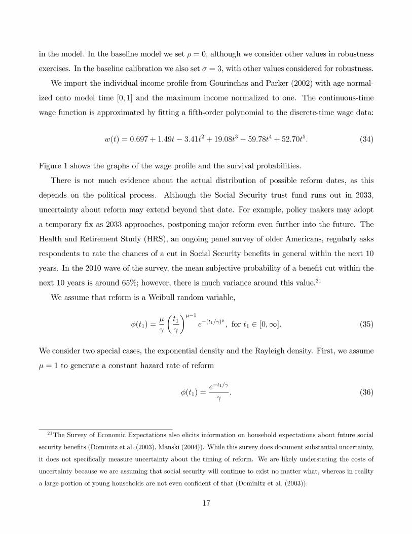
in the model. In the baseline model we set ρ = 0, although we consider other values in robustness

exercises. In the baseline calibration we also set σ = 3, with other values considered for robustness.

We import the individual income profile from Gourinchas and Parker (2002) with age normal-

ized onto model time [0, 1] and the maximum income normalized to one. The continuous-time

wage function is approximated by fitting a fifth-order polynomial to the discrete-time wage data:

w(t) = 0.697 + 1.49t− 3.41t2 + 19.08t3 − 59.78t4 + 52.70t5. (34)

Figure 1 shows the graphs of the wage profile and the survival probabilities.

There is not much evidence about the actual distribution of possible reform dates, as this

depends on the political process. Although the Social Security trust fund runs out in 2033,

uncertainty about reform may extend beyond that date. For example, policy makers may adopt

a temporary fix as 2033 approaches, postponing major reform even further into the future. The

Health and Retirement Study (HRS), an ongoing panel survey of older Americans, regularly asks

respondents to rate the chances of a cut in Social Security benefits in general within the next 10

years. In the 2010 wave of the survey, the mean subjective probability of a benefit cut within the

next 10 years is around 65%; however, there is much variance around this value.21

We assume that reform is a Weibull random variable,

φ(t1) =µ

γ

(t1γ

)µ−1e−(t1/γ)

µ

, for t1 ∈ [0,∞]. (35)

We consider two special cases, the exponential density and the Rayleigh density. First, we assume

µ = 1 to generate a constant hazard rate of reform

φ(t1) =e−t1/γ

γ. (36)

21The Survey of Economic Expectations also elicits information on household expectations about future social

security benefits (Dominitz et al. (2003), Manski (2004)). While this survey does document substantial uncertainty,

it does not specifically measure uncertainty about the timing of reform. We are likely understating the costs of

uncertainty because we are assuming that social security will continue to exist no matter what, whereas in reality

a large portion of young households are not even confident of that (Dominitz et al. (2003)).

17

Because it seems unlikely that the individual will totally escape reform, we calibrate this function

by assuming∫∞1

(e−t1/γ

)/γdt1 = 1%, which implies γ = −1/ ln 0.01.

Alternatively, it is plausible that political pressure for reform will mount as the trust fund

runs out of money by 2033. For this reason we will also consider a second calibration where

the likelihood of reform rises as the trust fund exhaustion date approaches. To capture this, we

compute φ′(t1) = 0 and set t1 = (2033− 2015)/75, which implies

γ =18

75

(µ

µ− 1

) 1µ

. (37)

The larger the value of µ, the greater the mass around 2033. Our computational procedure

struggles with values of µ larger than 2, so we set µ = 2 which then implies γ = 0.3394. Figure 2

shows the graphs of these two calibrations of φ(t1). We will report welfare calculations for both

calibrations.

The current Social Security policy (τ 1, b1) in the model is parameterized to match the current

policy in the US. Consistent with our modeling in earlier sections, we focus only on retirement

insurance (the Old Age and Survivors, or OASI, program) and ignore disability insurance. The

OASI payroll tax rate (combined employer and employee shares) is τ 1 = 10.6%. Benefits b1 are

chosen to match observed replacement rates for various income groups.

Social Security benefits are based on an individual’s Average IndexedMonthly Earnings (AIME),

calculated as average monthly earnings, indexed for economy-wide wage growth, over the highest

35 years of the individual’s career. A progressive benefit formula is applied to AIME to arrive

at an individual’s Primary Insurance Amount (PIA), the monthly benefit payable if benefits are

claimed at normal retirement age. Claiming before normal retirement age - for example, at age

65, as we assume in our model - results in an actuarial reduction to benefits. The progressive

benefit formula implies that the replacement rate - the ratio of monthly benefits to AIME - falls

with AIME.

The Social Security Trustees Report publishes replacement rates for several stylized workers,

each earning a fixed multiple of the economy-wide average wage throughout their career. According

to the 2013 Trustees Report, the very low income group, which earns 25% of the economy-wide

average wage, receives a replacement rate of 67.5% of AIME if benefits are claimed at age 65. The

18

low-income group, which earns 45% of the economy-wide average wage, has a replacement rate of

49.0% of AIME. The medium income group, which earns the economy-wide average wage, receives

a replacement rate of 36.4% of AIME. The high income group, which earns 1.6 times the average

wage, receives a replacement rate of 30.1% of AIME. Finally, workers who earn the maximum

taxable amount in each year of their career receive a replacement rate of 24.0% of AIME. These

replacement rates apply to the year 2055, when the 1990 cohort turns 65. To compute pre-reform

benefits, b1, we apply these replacement rates to the AIME for the normalized life-cycle income

profile in our model, which is 0.92927.22

For the policy experiments considered in the paper we assume that the reform undertaken will

balance the Social Security budget over the infinite horizon.23 According to Gokhale (2013) the

unfunded liabilities of the OASI program over the infinite horizon would require a permanent tax

increase of 3.1% of payroll (assuming no behavioral response to the tax increase). Alternatively,

all current and future benefits could be cut by 21%.24 As an initial pass, we consider both of these

possible reforms:

• Full benefit cut. An across-the-board reduction in benefits by 21% for all current and

future retirees (no exemption for current retirees) and no change in taxes. Hence, the new

policy is (τ 2, b2) = (τ 1, b1 × (1− 21%)).

• Full tax increase. An across-the-board increase in the OASI tax rate by 3.1 percentage

points for all taxpayers regardless of age and no change in benefits. Hence, (τ 2, b2) =

(τ 1 + 3.1%, b1).

We consider each of these reforms separately and assume that individuals know the reform

22In computing AIME for our life cycle model, we disregard wage indexation because the Gourinchas and Parker

(2002) real income profiles are already adjusted not only for price inflation, but also for cohort and time effects.23A partial reform may extend the horizon of the timing uncertainty, leaving the welfare costs that we consider

in the paper.24Of course, the required tax and benefit adjustments could be much different in a macroeconomic model that

includes household behavioral responses and factor price responses to demographic and fiscal shocks. For instance,

in Kitao (2014), the required tax increase is 6% and the required benefit cut is 33%. Our welfare costs go up when

we feed bigger policy shocks such as these into our model. In addition, the required tax and benefit adjustments

are slightly larger if reform is delayed, but these adjustments are so small that they can be ignored in our example.

19

that will occur, but they are uncertain about the timing. The results from these two scenarios

will clarify the intuition of how timing uncertainty influences individual consumption and savings

decisions. We will later consider the case where individuals are also uncertain about the structure

of reform, not knowing if it will be a benefit cut, a tax increase, or some combination of the two.

3.5. Results

In order to gain intuition about the effects of uncertainty about the timing of reform, we plot the

results for the benefit cut and tax increase scenarios. Figure 3 shows four consumption profiles

over the life cycle for the full benefit cut experiment, for an individual with average earnings who

faces a constant hazard rate of reform: the consumption path during the first stage c∗1; a pair

of hypothetical consumption paths during stage two, c∗2, conditional on reform at t1 = 0.5 and

t1 = 0.7 as an example; and the consumption profile from a world with no Social Security risk

where the individual gets her expected lifetime income, cNR, as a reference point. The path the

individual actually follows is c∗1 up to the stochastic date of reform and then consumption drops

down to c∗2. There is a continuum of many c∗2 paths, we have simply plotted two possibilities for

illustrative purposes. An important feature of the experiment to emphasize is that the individual

is still subject to a benefit cut even after the retirement date, so the first stage consumption path

takes this possibility into account. This figure clearly shows how uncertainty about the timing of

benefit reform causes non-trivial distortions to consumption-saving decisions. If the reform shock

is realized fairly early, then consumption falls below the level without Social Security risk, whereas

a later reform shock leaves consumption above the no-risk path. The trouble of course is that the

individual doesn’t know when the shock will hit.

Figure 4 plots the same information but for the case of a tax increase, again for an individual

with average earnings who faces a constant hazard rate of reform. We consider two alternative

hypothetical reform dates, t1 = 0.1 and t1 = 0.4 just as an example. We don’t plot reform

dates after retirement because, even though reform may indeed strike after retirement, there is no

distortion to consumption because the individual no longer pays Social Security taxes. Similar to

the case of a benefit cut, consumption always drops the moment reform strikes.

The drop in consumption in either scenario is not because the individual is taken by surprise

per se, but is instead the result of rational, forward-looking behavior in the face of uncertainty.

20

Reconsider Figure 3 and suppose the individual is standing just to the left of t = 0.7. From this

perspective, the individual knows the shock may happen at any time over the interval [0.7,∞] and

therefore bases consumption on that expectation, which is rational ex ante. But if the shock hits

at the next moment (i.e., at t = 0.7) then ex post the individual turns out to be a little poorer

than anticipated the moment before and hence consumption must be revised down.

Our first set of results corresponds to the welfare loss for an individual with average earnings

who faces a constant hazard rate of reform. We find that the magnitude of the welfare loss is

moderate for this individual: 0.01% of total lifetime consumption for the case of a benefit cut. We

also find that uncertainty about the timing of tax reform is twice as costly as uncertainty about

the timing of benefit reform, again for an individual with average earnings who faces a constant

hazard of reform.25 This is because the exponential density puts much of the mass during the

working period, so that if the individual is living in the benefit-reform world, then he actually

faces somewhat less uncertainty about his lifetime wealth because he knows there is a good chance

that benefits will be cut before he retires anyway.

We also find important distributional effects as we look beyond the average individual. Ta-

ble 1 reports welfare losses associated with uncertainty about the timing of reform for different

income levels (each relative to the average individual in the benefit reform scenario). Due to the

progressively of benefits, uncertainty about the timing of a benefit cut is more harmful to low

income individuals than to high income individuals. For example, Table 1 shows that, for the case

of constant hazard rate of reform (Panel A), the very low income group will experience a welfare

loss that is 4 times larger than what is experienced by the highest income group that maximizes

their social security contribution in each year of work. This asymmetry occurs because social

security benefits are a larger share of total retirement income for the poor than for the rich, and

uncertainty over something important is naturally going to be costly. Qualitatively, this result

continues to hold when we replace the exponential distribution with the Rayleigh distribution (see

Panel B).

But this distributional effect reverses its sign for the case of uncertainty about the timing of a

tax increase. Essentially, now the progressivity argument works in the opposite way. Even though

25While these numbers seem small, the fact that Social Security only taxes 10.6 percent of labor income implies

that it is only a limited part of individuals overall lifetime consumption.

21

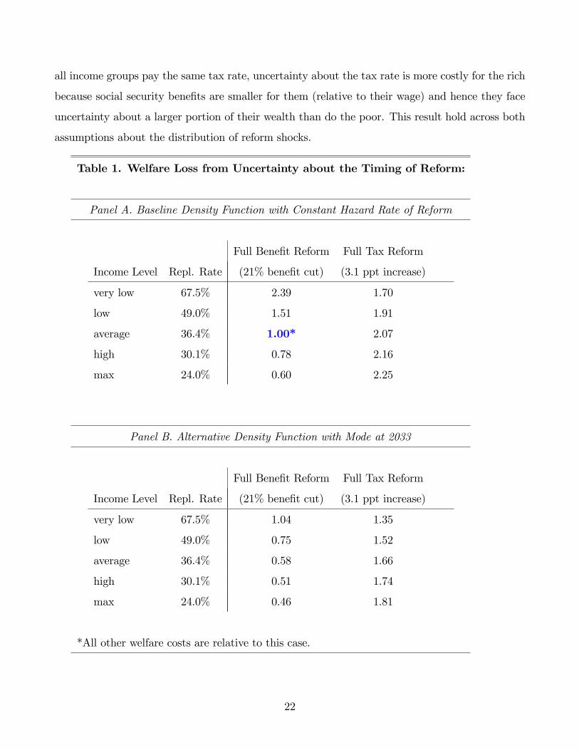
all income groups pay the same tax rate, uncertainty about the tax rate is more costly for the rich

because social security benefits are smaller for them (relative to their wage) and hence they face

uncertainty about a larger portion of their wealth than do the poor. This result hold across both

assumptions about the distribution of reform shocks.

Table 1. Welfare Loss from Uncertainty about the Timing of Reform:

Panel A. Baseline Density Function with Constant Hazard Rate of Reform

Full Benefit Reform Full Tax Reform

Income Level Repl. Rate (21% benefit cut) (3.1 ppt increase)

very low 67.5% 2.39 1.70

low 49.0% 1.51 1.91

average 36.4% 1.00* 2.07

high 30.1% 0.78 2.16

max 24.0% 0.60 2.25

Panel B. Alternative Density Function with Mode at 2033

Full Benefit Reform Full Tax Reform

Income Level Repl. Rate (21% benefit cut) (3.1 ppt increase)

very low 67.5% 1.04 1.35

low 49.0% 0.75 1.52

average 36.4% 0.58 1.66

high 30.1% 0.51 1.74

max 24.0% 0.46 1.81

*All other welfare costs are relative to this case.

22

4. Application 2: Timing and Structural Uncertainty

Now we present an application of Problem 2, where both the timing and structure of social security

reform are uncertain. First we introduce notation, household behavior, and welfare, and then we

compare simulated welfare costs from this application to the previous application with only timing

uncertainty.

4.1. Notation, Household Behavior, and Welfare

Let τ̃ 2 be the new tax rate that would be suffi cient to balance the budget without any reduction

in benefits, and likewise let b̃2 be the new benefit level that would balance the budget without a

tax increase. Of course, τ̃ 2 > τ 1 and b̃2 < b1. But the new policy that the government actually

chooses (τ 2, b2) is an uncertain, linear combination of these extremes. We will express the new

tax policy as a function of a continuous random variable α (with density θ(α) and sample space

[0, 1]):

τ 2(α) = τ 1 + α(τ̃ 2 − τ 1), (38)

b2(α) = b1 − (1− α)(b1 − b̃2), (39)

and

y2(t|α) =

(1− τ 2(α))w(t), for t ∈ [0, tR],

b2(α), for t ∈ [tR, T ].(40)

Using Theorem 2, the post-reform consumption path is

c∗2(t|t1, k(t1), α) =k(t1) +

∫ Tt1e−r(v−t1)y2(v|α)dv∫ T

t1e−r(v−t1)+(r−ρ)v/σΨ(v)1/σdv

e(r−ρ)t/σΨ(t)1/σ, for t ∈ [t1, T ], (41)

23

and the pre-reform Euler equation is

dc(t)

dt=

(c(t)σ+1

Ψ(t)

∫ 1

0

θ(α)

[k(t) +

∫ Tte−r(v−t)y2(v|α)dv∫ T

te−r(v−t)+(r−ρ)v/σΨ(v)1/σdv

]−σe(ρ−r)tdα− c(t)

)

×[σ

φ(t)

∫ ∞t

φ(t1)dt1

]−1+

[dΨ(t)

dt

1

Ψ(t)+ r − ρ

]c(t)

σ. (42)

Using this Euler equation, together with the law of motion and boundary conditions for the savings

account, we can compute the stage-one solution (c∗1(t), k∗1(t))t∈[0,T ].

Finally, for welfare comparisons, the no risk benchmark is

cNR(t) =

∫ 10

∫ T0θ(α)φ(t1)Y (t1|α)dt1dα +

[∫∞Tφ(t1)dt1

] ∫ T0e−rvy1(v)dv∫ T

0e−rv+(r−ρ)v/σΨ(v)1/σdv

e(r−ρ)t/σΨ(t)1/σ, t ∈ [0, T ],

(43)

where Y (t1|α) ≡∫ t10e−rvy1(v)dv +

∫ Tt1e−rvy2(v|α)dv, and the welfare cost of reform uncertainty ∆

solves the following equation

∫ T

0

e−ρtΨ(t)[cNR(t)(1−∆)]1−σ

1− σ dt (44)

=

∫ 1

0

∫ T

0

θ(α)φ(t1)

(∫ t1

0

e−ρtΨ(t)c∗1(t)

1−σ

1− σ dt+

∫ T

t1

e−ρtΨ(t)c∗2(t|t1, k∗1(t1), α)1−σ

1− σ dt

)dt1dα

+

[∫ ∞T

φ(t1)dt1

] ∫ T

0

e−ρtΨ(t)c∗1(t)

1−σ

1− σ dt.

In the absence of reliable data on expectations about the structure of future reform, which is

ultimately a political decision that will reflect the preferences of policymakers, we assume θ(α) is

the uniform density.

4.2. Results

Table 2 documents the welfare costs of double uncertainty for various income levels, each relative

to the average earner in the full benefit reform scenario with a constant hazard rate of reform. The

main finding of interest is that double uncertainty hurts the poor more than the rich by roughly

a factor of 3, regardless of which assumption we make about the distribution of reform dates.

24

Figures 5 through 7 show the effects of double uncertainty on consumption allocations over the

life cycle. In Figure 5 we report five consumption profiles: the optimal consumption path given

that reform has not yet happened, c∗1; the consumption path corresponding to a hypothetical

world without reform risk, cNR; and three post-reform consumption profiles c∗2 conditional on

reform striking at date t1 = 0.4. Note that reform may happen at any time of course. We are

just showing the optimal responses for this particular date. Furthermore, there is a continuum of

post-reform consumption profiles even for a single reform date because the structure of reform,

α, is a continuously distributed random variable as well. For illustrative purposes however, we

plot optimal responses to just three particular realizations α ∈ {0, 0.5, 1}, which correspond to

full benefit reform, 50-50 tax and benefit reform, and full tax reform. Our calculations of welfare

losses take into account the full distribution of α, rather than just the three realization shown

here, but the figure would be too messy to show all realizations over α.

Figure 5 illustrates that the individual will reduce consumption if the shock turns out to be

benefit reform, whereas consumption actually jumps up a bit if the shock takes the form of a tax

increase. This is because the individual was rationally planning for the contingency that benefits

would be dramatically cut, and hence the news that reform takes the structure of a tax increase

is a positive shock to expected wealth because there are only a few years of tax payments left and

now benefit are certain. To make the intuition clear, suppose at the very moment the individual

retires the government announces that the Social Security program will reform its budget solely

through increased taxation. This is a strictly positive wealth shock for this individual because

he/she doesn’t bear any of the burden of the tax increase, and now Social Security benefits are no

longer in jeopardy. But good news should not be confused with welfare, because the uncertainty

about the timing and structure of reform distort consumption and saving allocations in the years

leading up to reform, even if reform just so happens to never actually end up costing the individual

anything.

Figure 6 plots the exact same information as Figure 5, but for the case of a later realization of

the reform shock (t1 = 0.6 instead of 0.4). Taken together, the two figures show similar qualiti-

tative responses to the resolution of timing and structural uncertainty. However, the individual’s

responses are more exaggerated in the case of the later shock, at least up to a certain age, after

which there is eventually so little remaining Social Security benefits to collect that uncertainty

25

about the timing and structure of reform becomes irrelevant.

Figure 7 shows a little more detail. We add to Figures 5 and 6 the optimal consumption

responses to a wider variety of realizations of the timing of reform, t1 ∈ {0.2, 0.3, ..., 0.8, 0.9},

while still plotting just three particular realizations of the structure of reform α ∈ {0, 0.5, 1}. This

figure helps to illustrate, at a glance, a few of the many contingent consumption plans formulated

by the individual, and it helps to illustrate the breath of the distortion to consumption that is

caused by the presence of double uncertainty about Social Security reform. For instance, at this

particular parameterization, the variation in consumption during the middle part of the retirement

period is especially severe. The maximum possible consumption levels over retirement result from

the cases in which full tax reform (with no benefit cut) strikes during retirement and the individual

therefore realized that he is totally offthe hook, while minimum possible consumption levels during

the retirement period result from cases in which full benefit reform strikes near the transition from

work to retirement.

26

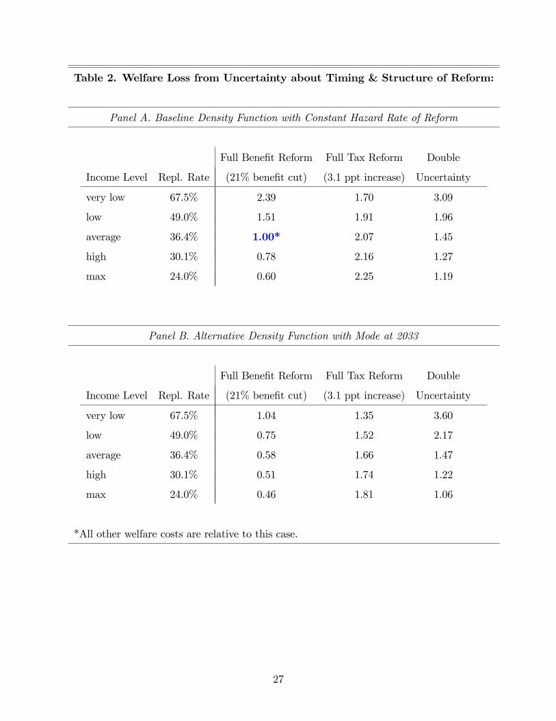
Table 2. Welfare Loss from Uncertainty about Timing & Structure of Reform:

Panel A. Baseline Density Function with Constant Hazard Rate of Reform

Full Benefit Reform Full Tax Reform Double

Income Level Repl. Rate (21% benefit cut) (3.1 ppt increase) Uncertainty

very low 67.5% 2.39 1.70 3.09

low 49.0% 1.51 1.91 1.96

average 36.4% 1.00* 2.07 1.45

high 30.1% 0.78 2.16 1.27

max 24.0% 0.60 2.25 1.19

Panel B. Alternative Density Function with Mode at 2033

Full Benefit Reform Full Tax Reform Double

Income Level Repl. Rate (21% benefit cut) (3.1 ppt increase) Uncertainty

very low 67.5% 1.04 1.35 3.60

low 49.0% 0.75 1.52 2.17

average 36.4% 0.58 1.66 1.47

high 30.1% 0.51 1.74 1.22

max 24.0% 0.46 1.81 1.06

*All other welfare costs are relative to this case.

27

5. Robustness

In this section we show how our results change when we alter certain assumptions. First, we

consider different assumptions about preference parameters (the coeffi cient of risk aversion and

the discount rate). Second, we show how much larger the welfare costs of uncertainty can be

as we increase the variance of timing uncertainty and as we increase the variance of structural

uncertainty. These are important extensions because we do not have good data to guide our

baseline calibration of timing and structural uncertainty. Third, we show that the poor are still

hit much harder than the rich by reform uncertainty even if we consider differential mortality

across income groups, which is commonly believed to unwind at least some of the progressivity of

Social Security (e.g., Coronado et al. (1999)).

5.1. Preference Parameters

As we increase the coeffi cient of relative risk aversion, σ, from the baseline value of 3 up to 5,

the magnitude of the welfare cost of reform uncertainty increases dramatically. For instance, for

the baseline case of exponentially distributed uncertainty about the timing of a full benefit cut,

the cost to an average earner increases by more than 50%. The same is also true for the case of

exponentially distributed uncertainty about the timing of a full tax increase.

Our baseline assumption is that the individual only discounts for mortality and not for pure

time preference (ρ = 0). If we make a slightly more standard assumption that the discount rate

equals the market rate of interest (ρ = r = 2.9%), then the welfare effects of uncertainty about

reform grow stronger. For instance, for the baseline case of exponentially distributed uncertainty

about the timing of a full benefit cut, the cost of uncertainty for an average earner increases by

almost 30%, while uncertainty about the timing of a full tax increase becomes almost 10% more

costly to an average earner.

5.2. Uniform Reform Dates

A plausible assumption is that the random reform date is distributed uniformly over the indi-

vidual’s maximum lifespan, φ(t1) = 1 for all t1 ∈ [0, 1]. Such an assumption spreads out the

distribution of reform shocks more than in the baseline densities. The welfare results are reported

28

in Table 3, holding everything else at baseline parameters and assuming the structure of reform

(α) continues to be distributed uniformly as well. Uncertainty about the timing of full benefit

reform is now much more costly than in the baseline cases, while the cost of uncertainty about

the timing of full tax reform is on the same order of magnitude as the baseline cases. Double

uncertainty now hits the poor almost 4 times as hard as it hits the rich.

Table 3. Welfare Loss from Uncertainty about Timing & Structure of Reform:

Uniform Distribution of Reform Dates over Max Lifespan

Full Benefit Reform Full Tax Reform Double

Income Level Repl. Rate (21% benefit cut) (3.1 ppt increase) Uncertainty

very low 67.5% 10.66 1.65 7.23

low 49.0% 6.33 1.83 4.53

average 36.4% 3.84 1.97 3.02

high 30.1% 2.77 2.05 2.40

max 24.0% 1.88 2.13 1.88

All welfare costs are relative to the numeraire case in Panel A of Table 2.

5.3. Extreme Political Risk

We have thus far used a uniform distribution over α (the structural uncertainty parameter) in all

of our calculations for the double uncertainty case. This assumption implies that any particular

convex combination (compromise) between a full tax increase and a full benefit cut is just as

likely as any other combination. This may be a reasonable baseline assumption, but it could be

the case that the structure of reform will ultimately look more like the outcome of a tug-of-war

contest between two political parties, with one side winning completely and the other side losing,

rather than a compromise.26 In this subsection we assume that the structure of reform is uncertain

26See Baker et al. (2014) for a discussion of political polarization in recent years in American politics. Also see

Davig and Foerster (2014) for a similar discussion.

29

and will be either all on the tax side or all on the benefit side, with no probability of a convex

combination. We assume that these two possibilities are equally likely, and we leave everything

else at the baseline parameterization.

We obtain two key results. First, extreme political risk causes the welfare costs of reform

uncertainty to be significantly larger than in the baseline calculations, for all income groups.

Second, extreme political risk widens the inequality in welfare costs among the rich and poor. In

the baseline calculations, reform uncertainty hits the poor about 3 times harder than the rich, but

in the current case it is closer to a factor of 4.

5.4. Differential Mortality

It is well known that low-income individuals suffer from lower survival probabilities at all ages

relative to high-income individuals. We have recomputed our welfare analysis for the case of

income-specific survival functions based on Social Security administrative data provided in Chart

1 of Waldron (2013). These data suggest that among 63-year-old males, the death rate of the first,

third, eighth and tenth lifetime income deciles are, respectively, 2.6, 1.3, 0.8, and 0.6 times that

of the average of the fifth and sixth deciles.27 Based on this, we assume that throughout their

lives, maximum earners face age-specific hazard rates of dying that are 0.6 times those of average

earners, high earners face age-specific hazard rates that are 0.8 times those of average earners, low

earners face age-specific hazard rates that are 1.3 times those of average earners, and very low

earners face age-specific hazard rates that are 2.6 times those of average earners. (If scaling by

these factors causes an age-specific hazard rate to exceed 1, that hazard rate is set to 1). Allowing

hazard rates to differ by income group causes almost no change to our calculations of the welfare

costs of uncertainty about the timing of reform.

Why doesn’t differential mortality undo our results? One may think that because our results

are driven by the progressivity of the Social Security system, including differential mortality would

undo our results since this would unwind (or even reverse) the progressivity of the system. While it

is true that differential mortality unwinds the progressivity of Social Security in a cross-sectional

27These relative death rates likely understate the extent of differential mortality as the sample in Waldron (2013)

excludes disabled individuals, individuals who have not accumulated the 10 years of earnings required to qualify

for Social Security, and individuals who do not survive to age 63.

30

sense, it does not unwind the progressivity in a longitudinal sense. At a moment in time, the

ratio of aggregate benefits collected by survivors to aggregate taxes paid by workers would tend

to be low for segments of the population with lower survival probabilities. But this has nothing

to do with how a given worker treats Social Security taxes and benefits in an expected utility

(longitudinal) model. In such a model, the progressivity of Social Security is only related to the

benefit-earning rule and not to mortality risk, because the latter enters the model only though

the discount factor in the utility function. Regardless of their survival type, expected utility

maximizers make an optimal consumption-saving plan that accounts for the contingency that

they survive until the maximum possible date. In other words, income flows (like Social Security)

in the budget constraint of an expected utility maximizer are not discounted for survival risk.

6. Conclusion

In this paper we attempt to understand the welfare consequences of uncertainty over the timing and

structure of social security reform. Household decision-making in the face of reform uncertainty

can be modeled as a stochastic two-stage optimal control problem. We have formalized the tools

that are required for studying this issue in a continuous-time setting.

We have paid special attention to how these welfare costs are distributed across income groups.

While the precise magnitude of the welfare costs depend on a variety of factors, a consistent theme

throughout our paper is that reform uncertainty may strike low-income groups especially hard.

While the need for reform itself is driven by unavoidable demographic forces, uncertainty about

the timing and structure of reform are avoidable. All of the costs that we report in this paper go

away if policymakers simply announce when and how Social Security will be reformed.

31

References

Abel, Andrew B. and Janice C. Eberly, “Investment, Valuation, and Growth Options,”

Quarterly Journal of Finance, 2012, 2 (1).

Amit, Raphael, “Petroleum Reservoir Exploitation: Switching from Primary to Secondary Re-

covery,”Operations Research, 1986, 34 (2), 534—549.

Baker, Scott R., Nicholas Bloom, and Steven Davis, “Measuring Economic Policy Uncer-

tainty,”Working Paper, Stanford May 2013.

, , Brandice Canes-Wrone, Steven J. Davis, and Jonathan Rodden, “Why Has US

Policy Uncertainty Risen Since 1960?,”American Economic Review: Papers and Proceedings,

May 2014, 104 (5), 56—60.

Belo, Frederico, Vito D. Gala, and Jun Li, “Government Spending, Political Cycles, and

the Cross-Section of Stock Returns,”Working Paper October 2011.

Benítez-Silva, Hugo, Debra S. Dwyer, Frank Heiland, and Warren C. Sanderson,

“Retirement and Social Security Reform Expectations: A Solution to the New Early Retirement

Puzzle,”Working Paper, Stony Brook 2007.

Bernanke, Ben S., “Irreversibility, Uncertainty, and Cyclical Investment,”Quarterly Journal of

Economics, 1983, 98 (1), 85—106.

Blundell, Richard and Thomas M. Stoker, “Consumption and the Timing of Income Risk,”

European Economic Review, 1999, 43, 475—507.

Boucekkine, Raouf, Aude Pommeret, and Fabien Prieur, “Optimal Regime Switching

and Threshold Effects: Theory and Application to a Resource Extraction Problem under Irre-

versibility,”Working Papers, LAMETA, Universtiy of Montpellier 2012.

, , and , “On the timing and optimality of capital controls: Public expenditures, debt

dynamics and welfare,”International Journal of Economic Theory, 2013, 9 (1), 101—112.

32

, , and , “Technological vs. Ecological Switch and the Environmental Kuznets Curve,”

American Journal of Agricultural Economics, 2013, 95 (2), 252—260.

, Cagri Saglam, and Thomas Vallee, “Technology Adoption Under Embodiment: A Two-

Stage Optimal Control Approach,”Macroeconomic Dynamics, April 2004, 8 (02), 250—271.

Boutchkova, Maria, Hitesh Doshi, Art Durnev, and Alexander Molchanov, “Precarious

Politics and Return Volatility,”Review of Financial Studies, 2012, 25 (4), 1111—1154.

Bütler, Monika, “Anticipation Effects of Looming Public-Pension Reforms,”Carnegie-Rochester

Conference Series on Public Policy, 1999, 50 (1), 119—159.

Clarke, Harry R. andWilliam J. Reed, “Consumption/Pollution Tradeoffs in an Environment

Vulnerable to Pollution-Related Catastrophic Collapse,” Journal of Economic Dynamics and

Control, 1994, 18, 991—1010.

Coronado, Julia Lynn, Don Fullerton, and Thomas Glass, “Distributional Impacts of

Proposed Changes to the Social Security System,”NBER Working Paper, National Bureau of

Economic Research January 1999.

Croce, M. Max, Howard Kung, Thien T. Nguyen, and Lukas Schmid, “Fiscal Policies

and Asset Prices,”Review of Financial Studies, 2012, 25 (9), 2635—2672.

Dasgupta, Partha and Geoffrey Heal, “The Optimal Depletion of Exhaustible Resources,”

Review of Economic Studies, 1974, 41, 3—28.

Davig, Troy and Andrew Foerster, “Uncertainty and Fiscal Cliffs,”Working Paper, Federal

Reserve Bank of Kansas City April 2014.

Diamond, Peter and Jonathan Gruber, “Social Security and Retirement in the United

States,”NBER Working Paper, National Bureau of Economic Research January 1999.

Dogan, Erol, Cuong Le Van, and Cagri Saglam, “Optimal Timing of Regime Switching in

Optimal Growth Models: A Sobolev Space Approach,”Mathematical Social Sciences, 2011, 61,

97—103.

33

Dominitz, Jeff, Charles F. Manski, and Jordan Heinz, “Will Social Security be There for

You?: How Americans Perceive their Benefits,”NBER Working Papers 9798, National Bureau

of Economic Research, Inc 2003.

Durnev, Art, “The Real Effects of Political Uncertainty: Elections and Investment Sensitivity

to Stock Prices,”Working Paper September 2010.

Eeckhoudt, Louis, Christian Gollier, and Nicolas Treich, “Optimal Consumption and the

Timing of the Resolution of Uncertainty,”European Economic Review, 2005, 49, 761—773.

Epstein, Larry G., Emmanuel Farhi, and Tomasz Strzalecki, “How Much Would You Pay

to Resolve Long-Run Risk,”American Economic Review, 2014, forthcoming.

Evans, Richard W., Laurence J. Kotlikoff, and Kerk L. Phillips, “Game Over: Simulat-

ing Unsustainable Fiscal Policy,”NBER Working Papers 17917, National Bureau of Economic

Research, Inc 2012.

Fernández-Villaverde, Jesús, Pablo Guerrón-Quintana, Keith Kuester, and Juan

Rubio-Ramírez, “Fiscal Volatility Shocks and Economic Activity,”Working Paper April 2013.

Gokhale, Jagadeesh, “Social Security Reform: Does Privatization Still Make Sense?,”Harvard

Journal on Legislation, 2013, 50, 169—207.

Gomes, Francisco J., Laurence J. Kotlikoff, and Luis M. Viceira, “The Excess Burden of

Government Indecision,”NBERWorking Papers 12859, National Bureau of Economic Research,

Inc 2007.

Gourinchas, Pierre-Olivier and Jonathan A. Parker, “Consumption Over the Life Cycle,”

Econometrica, January 2002, 70 (1), 47—89.

Hassett, Kevin A. and Gilbert E. Metcalf, “Investment with Uncertain Tax Policy: Does

Random Tax Policy Discourage Investment?,”The Economic Journal, 1999, 109 (457), 372—393.

Hoel, Michael, “Resource Extraction when a Future Substitute has an Uncertain Cost,”Review

of Economic Studies, 1978, 45 (3), 637—644.

34

Hugonnier, Julien, Florian Pelgrin, and Aude Pommeret, “Technology Adoption under

Uncertainty in General Equilibrium,”Working Paper 2006.

Julio, Brandon and Youngsuk Yook, “Political Uncertainty and Corporate Investment Cy-

cles,”Working Paper 2012.

Kamien, Morton I. and Nancy L. Schwartz, “Optimal Maintenance and Sale Age for a

Machine Subject to Failure,”Management Science, 1971, 17 (8), 495—504.

Kemp, Murray C. and Ngo Van Long, “Optimal Control Problems with Integrands Discon-

tinuous with Respect to Time,”The Economic Record, June-Sept 1977, 53 (142&143), 405—20.

Kitao, Sagiri, “Sustainable Social Security: Four Options,”Review of Economic Dynamics, 2014,

17 (4), 756—779.

Liebman, Jeffrey B. and Erzo F.P. Luttmer, “Would People Behave Differently If They

Better Understood Social Security? Evidence From a Field Experiment,”American Economic

Journal: Economic Policy, 2014, forthcoming.

Luttmer, Erzo F. P. and Andrew A. Samwick, “The Welfare Cost of Perceived Policy

Uncertainty: Evidence from Social Security,”Working Paper, Dartmouth College 2012.

Makris, Miltiadis, “Necessary conditions for infinite-horizon discounted two-stage optimal con-

trol problems,” Journal of Economic Dynamics and Control, December 2001, 25 (12), 1935—

1950.

Mangasarian, Olvi L., “Suffi cient Conditions for the Optimal Control of Nonlinear Systems,”

SIAM Journal on Control, 1966, 4 (1), 139—152.

Manski, Charles F., “Measuring Expectations,”Econometrica, 2004, 72 (5), 1329—1376.

McGrattan, Ellen R. and Edward C. Prescott, “On Financing Retirement with an Aging

Population,”Working Paper, University of Minnesota 2014.

Pantzalis, Christos, David A. Strangeland, and Harry J. Turtle, “Political elections and

the resolution of uncertainty: The international evidence,” Journal of Banking and Finance,

2000, 24 (10), 1575—1604.

35

Pastor, Lubos and Pietro Veronesi, “Political Uncertainty and Risk Premia,”Working Paper

September 2011.

Pommeret, Aude and Katheline Schubert, “Abatement Technology Adoption Under Uncer-

tainty,”Macroeconomic Dynamics, 2009, 13 (04), 493—522.

Rodrik, Dani, “Policy Uncertainty and Private Investment in Developing Countries,” NBER

Working Papers 2999, National Bureau of Economic Research June 1989.

Saglam, Cagri, “Optimal Pattern of Technology Adoptions under Embodiment: A Multi-Stage

Optimal Control Approach,”Optimal Control Applications and Methods, 2011, 32, 574—586.

Sargent, Thomas, “Ambiguity in American Monetary and Fiscal Policy,”Working Paper, New

York University May 2005.

Sialm, Clemens, “Stochastic taxation and asset pricing in dynamic general equilibrium,”Journal

of Economic Dynamics and Control, 2006, 30 (3), 511—540.

Stokey, Nancy L., “Wait-and-See: Investment Options under Policy Uncertainty,” Working

Paper, University of Chicago April 2014.

Tahvonen, Olli and Cees Withagen, “Optimality of Irreversible Pollution Accumulation,”

Journal of Economic Dynamics and Control, 1996, 20, 1775—1795.

Tomiyama, Ken, “Two-stage optimal control problems and optimality conditions,”Journal of

Economic Dynamics and Control, 1985, 9 (3), 317—337.

Ulrich, Maxim, “How Does the Bond Market Perceive Government Interventions?,”Working

Paper May 2012.

van der Wiel, Karen, “Preparing for Policy Changes: Social Security Expectations and Pension

Scheme Participation,”IZA DP No. 3623, Institute for the Study of Labor 2008.

Waldron, Hilary, “Mortality Differentials by Lifetime Earnings Decile: Implications for Evalu-

ations of Proposed Social Security Law Changes,”Social Security Bulletin, 2013, 73 (1).

36

Wright, Ian, Nick Bloom, and Jose Barrero, “Investment and the Term Structure of Uncer-

tainty,”Working Paper, Stanford University 2014.

37

Appendices

Appendix A provides a detailed proof of Theorem 1. Appendix B provides a full derivation of

the solution to the household’s optimization problem.

Appendix A: Proof of Theorem 1

Step 1. This step of the backward induction procedure is a completely standard Pontryagin

problem and needs very little justification. The optimal control and state paths after the switch

is realized must solve a standard deterministic control problem. We denote the solution to this

subproblem (u∗2(t|t1, x(t1)), x∗2(t|t1, x(t1)))t∈[t1,T ], where the extra notation is meant to convey the

dependence of the solution on the switch date t1 and on the state variable at that date x(t1). The

last part of Step 1 is strictly for convenience: we take this solution and change the time dummy

t to z, and change the switch point t1 to t and write (u∗2(z|t, x(t)), x∗2(z|t, x(t)))z∈[t,T ]. Thus we

have the optimal control and state paths for all points in time z greater than switch point t. This

change of dummies is innocuous but proves to be very helpful below in the process of linking the

subproblems together though the continuation functional in the next step.

Step 2. This step requires a little more explanation. The purpose of this step is to find the

optimal paths for the control and state before the realization of the switch. Hence, using the

solution from Step 1, the objective functional is

maxu(t)t∈[0,T ]

: J1 = E[∫ t1

0

f1(t, u(t), x(t))dt+

∫ T

t1

f2(t, u∗2(t|t1, x(t1)), x

∗2(t|t1, x(t1)))dt

](A1)

or

maxu(t)t∈[0,T ]

: J1 =

∫ T

0

∫ t1

0

φ(t1)f1(t, u(t), x(t))dtdt1 +

∫ T

0

φ(t1)S(t1, x(t1))dt1 (A2)

+

∫ ∞T

∫ T

0

φ(t1)f1(t, u(t), x(t))dtdt1,

where S(t1, x(t1)) is the continuation value or continuation function,

S(t1, x(t1)) =

∫ T

t1

f2(t, u∗2(t|t1, x(t1)), x

∗2(t|t1, x(t1)))dt, (A3)

38

and likewise∫ T0φ(t1)S(t1, x(t1))dt1 is the continuation functional. The constraints are

dx(t)

dt= g1(t, u(t), x(t)), for t ∈ [0, T ] , (A4)

x(0) = x0, x(T ) = xT . (A5)

Note that the control and state variables are defined over the entire planning interval because

the switch could happen at any time on this interval, and hence the pre-switch problem amounts

to choosing a path for these variables over the full interval. The marginal valuation of the state

variable reflects the fact that the switch could happen at any moment in time, and hence the

entire timepath of the state variable is relevant in determining the continuation value during the

second stage. This makes matters more complicated than in the standard two-stage model with a

deterministic switch, because there the costate variables from the two stages are simply equated

at the switch point to ensure that the value of finishing the first stage with an extra unit of the

state variable is equal to the value of starting the second stage with another unit. Whereas here

the two stages are linked together through a continuation functional. The solution to the above

problem is the one that will be followed up to the random switch point.

This appears to be a non-standard control problem, but with some algebra we can convert it

into a standard one for which the standard Maximum Principle applies. To make progress, let’s

change the dummy of integration in the second integral in J1 from t1 to t, and also change the

dummy in the continuation functional from t to z. Now we restate the objective functional as

maxu(t)t∈[0,T ]

: J1 =

∫ T

0

∫ t1

0

φ(t1)f1(t, u(t), x(t))dtdt1 +

∫ T

0

φ(t)S(t, x(t))dt (A6)

+

∫ ∞T

∫ T

0

φ(t1)f1(t, u(t), x(t))dtdt1,

where

S(t, x(t)) =

∫ T

t

f2(z, u∗2(z|t, x(t)), x∗2(z|t, x(t)))dz. (A7)

This innocuous change of variables is helpful because it allows us to write the continuation function

S as a function of x(t). In doing so, u∗2(z|t, x(t)) and x∗2(z|t, x(t)) now take on the interpretation

of the optimal control and state variables for all points in time z that are beyond the switch date

39

t and conditional on x(t).

Changing the order of integration in the first term in J1, along with applying Fubini’s Theorem

to the third term in J1, causes a more manageable Pontryagin problem to emerge. Let us now

restate our problem one last time

maxu(t)t∈[0,T ]

: J1 =

∫ T

0

{[∫ ∞t

φ(t1)dt1

]f1(t, u(t), x(t)) + φ(t)S(t, x(t))

}dt, (A8)

subject to

S(t, x(t)) =

∫ T

t

f2(z, u∗2(z|t, x(t)), x∗2(z|t, x(t)))dz, (A9)

dx(t)

dt= g1(t, u(t), x(t)), for t ∈ [0, T ], (A10)

x(0) = x0, x(T ) = xT . (A11)

This reformulated objective functional has an intuitive interpretation. The first term in the in-

tegrand gives the payoff of u(t) and x(t) through the function f1(t, u(t), x(t)), weighted by the

probability that the random switch will occur sometime after t. The second term gives the payoff

of holding x(t) through the continuation value S(t, x(t)), weighted by the density function φ(t).

Thus, the first payoff term f1 is weighted by one minus the c.d.f. because this payoff is relevant

as long as the switch comes later than t, whereas the second payoff term S is weighted by the

p.d.f. because this payoff is relevant only at the switch point. The standard Maximum Princi-

ple can be applied to this reformulated subproblem. We denote the solution to this subproblem

(u∗1(t), x∗1(t))t∈[0,T ]. This is the solution path for all t before the realization of the random switch.

Note that the switch could happen at any point in time. This is why this subproblem is defined

over the entire planning interval.

Appendix B. Derivation of Solution to Household Problem

Using Theorem 1 as our guide, we can solve the stochastic two-stage household problem recursively

by breaking it into two Pontryagin subproblems as follows.

Step 1. Solve the post-reform (t = t1) subproblem:

We first solve the Pontryagin subproblem corresponding to the moment that reform occurs.

40

This is a deterministic, fixed endpoint control problem

maxc(t)t∈[t1,T ]

: J2 =

∫ T

t1

e−ρtΨ(t)c(t)1−σ

1− σ dt, (B1)

subject todk(t)

dt= rk(t) + y2(t)− c(t), for t ∈ [t1, T ], (B2)

t1 given, k(t1) given, k(T ) = 0. (B3)

Form the Hamiltonian H2 with multiplier λ2(t)t∈[t1,T ] and compute the necessary conditions

H2 = e−ρtΨ(t)c(t)1−σ

1− σ + λ2(t)[rk(t) + y2(t)− c(t)], (B4)

∂H2∂c(t)

= e−ρtΨ(t)c(t)−σ − λ2(t) = 0, for t ∈ [t1, T ], (B5)

dλ2(t)

dt= − ∂H2

∂k(t)= −rλ2(t), for t ∈ [t1, T ]. (B6)

Rewrite the costate equation

λ2(t) = λ2(t1)e−r(t−t1), (B7)

and collapse the necessary conditions into a single equation

e−ρtΨ(t)c(t)−σ = λ2(t1)e−r(t−t1). (B8)

Solve for c(t)

c(t) = λ2(t1)−1/σe[(r−ρ)t−rt1]/σΨ(t)1/σ. (B9)

Solve differential equation (B2) using the boundary conditions in (B3)

k(t1) +

∫ T

t1

y2(v)e−r(v−t1)dv =

∫ T

t1

c(v)e−r(v−t1)dv. (B10)

Insert (B9) into (B10)

k(t1) +

∫ T

t1

y2(v)e−r(v−t1)dv =

∫ T

t1

λ2(t1)−1/σe−r(v−t1)+[(r−ρ)v−rt1]/σΨ(v)1/σdv, (B11)

41

and solve for the constant

λ2(t1)−1/σ =

k(t1) +∫ Tt1y2(v)e−r(v−t1)dv∫ T

t1e−r(v−t1)+[(r−ρ)v−rt1]/σΨ(v)1/σdv

. (B12)

Insert this into (B9) to obtain the solution consumption path

c∗2(t|t1, k(t1)) =k(t1) +

∫ Tt1e−r(v−t1)y2(v)dv∫ T

t1e−r(v−t1)+(r−ρ)v/σΨ(v)1/σdv

e(r−ρ)t/σΨ(t)1/σ, for t ∈ [t1, T ]. (B13)

This is the optimal consumption path after the reform shock has hit.

Anticipating the method for solving the pre-reform subproblem in the next step of Theorem

1, we will need to change the time dummies: now think of t as the reform date and z as any time

after the reform date. Thus, rewrite the solution as

c∗2(z|t, k(t)) =k(t) +

∫ Tte−r(v−t)y2(v)dv∫ T

te−r(v−t)+(r−ρ)v/σΨ(v)1/σdv

e(r−ρ)z/σΨ(z)1/σ, for z ∈ [t, T ]. (B14)

Step 2. Solve the pre-reform (t = 0) subproblem:

Next we solve the t = 0 subproblem as in Theorem 1,

maxc(t)t∈[0,T ]

: J1 =

∫ T

0

{[∫ ∞t

φ(t1)dt1

]e−ρtΨ(t)

c(t)1−σ

1− σ + φ(t)S(t, k(t))

}dt, (B15)

subject to

S(t, k(t)) =

∫ T

t

e−ρzΨ(z)c∗2(z|t, k(t))1−σ

1− σ dz

=1

1− σ

[k(t) +

∫ Tte−r(v−t)y2(v)dv∫ T

te−r(v−t)+(r−ρ)v/σΨ(v)1/σdv

]1−σ ∫ T

t

e[r(1−σ)−ρ]z/σΨ(z)1/σdz, (B16)

dk(t)

dt= rk(t) + y1(t)− c(t), for t ∈ [0, T ], (B17)

k(0) = 0, k(T ) = 0. (B18)

42

Form the Hamiltonian H1 with multiplier λ1(t)t∈[0,T ] and compute the necessary conditions28

H1 =

[∫ ∞t

φ(t1)dt1

]e−ρtΨ(t)

c(t)1−σ

1− σ + φ(t)S(t, k(t)) + λ1(t)[rk(t) + y1(t)− c(t)], (B19)

∂H1∂c(t)

=

[∫ ∞t

φ(t1)dt1

]e−ρtΨ(t)c(t)−σ − λ1(t) = 0, for t ∈ [0, T ], (B20)

dλ1(t)

dt= − ∂H1

∂k(t)= −φ(t)

[k(t) +

∫ Tte−r(v−t)y2(v)dv∫ T

te−r(v−t)+(r−ρ)v/σΨ(v)1/σdv

]−σe−rt − rλ1(t), for t ∈ [0, T ]. (B21)

Differentiate (B20) with respect to t

0 = −φ(t)e−ρtΨ(t)c(t)−σ +

[∫ ∞t

φ(t1)dt1

] [dΨ(t)

dte−ρt − ρΨ(t)e−ρt

]c(t)−σ

−[∫ ∞

t

φ(t1)dt1

]σe−ρtΨ(t)c(t)−σ−1

dc(t)

dt− dλ1(t)

dt. (B22)

Insert (B20) into (B21)

dλ1(t)

dt= −φ(t)

[k(t) +

∫ Tte−r(v−t)y2(v)dv∫ T

te−r(v−t)+(r−ρ)v/σΨ(v)1/σdv

]−σe−rt − r

[∫ ∞t

φ(t1)dt1

]e−ρtΨ(t)c(t)−σ, (B23)

and then insert (B23) into (B22) to obtain the Euler equation

dc(t)

dt=

(c(t)σ+1

Ψ(t)

[k(t) +

∫ Tte−r(v−t)y2(v)dv∫ T

te−r(v−t)+(r−ρ)v/σΨ(v)1/σdv

]−σe(ρ−r)t − c(t)

)×[σ

φ(t)

∫ ∞t

φ(t1)dt1

]−1+

[dΨ(t)

dt

1

Ψ(t)+ r − ρ

]c(t)

σ. (B24)

28The necessary conditions are also suffi cient because the integrand of J1 is concave in c(t) and k(t) (see Corollary

1).

43

0 0.2 0.4 0.6 0.8 10

0.5

1

age, t

Figure 1. Baseline Wage Profile and Survival Uncertainty

Survival data: SSA 1990 cohort. Wage data: Gourinchas and Parker (2002).

Ψ(t)w(t)

0 0.2 0.4 0.6 0.8 10

0.5

1

1.5

2

2.5

3

3.5

4

4.5

reform date, t1

pdf,φ(t

1)

Figure 2. Weibull Density Functions over Random Timing of Reform

baseline

alternative

0 0.2 0.4 0.6 0.8 10.5

0.6

0.7

0.8

age, t

consumption,c(t)

Figure 3. The Case of Benefit Reform with Stochastic Reform Date

tR = 0.53

Social security parameters: τ1 = 0.106, τ2 = 0.106, b1 = 0.322, b2 = 0.254.

c∗

1(t)hypothetical reformdate t1 = 0.7 c

∗

2(t|0.7)

c∗

2(t|0.5)hypothetical reformdate t1 = 0.5

cNR(t)

0 0.2 0.4 0.6 0.8 10.5

0.55

0.6

0.65

0.7

0.75

0.8

0.85

age, t

consumption,c(t)

Figure 4. The Case of Tax Reform with Stochastic Reform Date

tR = 0.53

c∗

1(t)

Social security parameters: τ1 = 0.106, τ2 = 0.137, b1 = 0.322, b2 = 0.322.

hypotheticalreform date t1 = 0.4

hypotheticalreform datet1 = 0.1

c∗

2(t|0.4)

c∗

2(t|0.1)

cNR(t)

0 0.2 0.4 0.6 0.8 10.4

0.45

0.5

0.55

0.6

0.65

0.7

0.75

0.8

0.85

0.9

0.95

age, t

consumption,c(t)

Figure 5. Double Uncertainty: Timing and Structural Uncertainty

tR = 0.53

The share of the budget crisis resolved through extra taxation is α,and the share resolved through benefit adjustments is 1 −α.

c∗

1(t)

cNR(t)

hypotheticalreformdate t1 = 0.4

c∗

2(t|0.4)α=1

c∗

2(t|0.4)α=0.5

c∗

2(t|0.4)α=0

0 0.2 0.4 0.6 0.8 10.4

0.45

0.5

0.55

0.6

0.65

0.7

0.75

0.8

0.85

0.9

.95

age, t

consumption,c(t)

Figure 6. Double Uncertainty: Timing and Structural Uncertainty

tR = 0.53

The share of the budget crisis resolved through extra taxation is α,and the share resolved through benefit adjustments is 1 −α.

c∗

1(t)

cNR(t)

hypothetical reformdate t1 = 0.6

c∗

2(t|0.6)α=0.5

c∗

2(t|0.6)α=1

c∗

2(t|0.6)α=0

0 0.2 0.4 0.6 0.8 10.4

0.45

0.5

0.55

0.6

0.65

0.7

0.75

0.8

0.85

age, t

consumption,c(t)

Figure 7. Double Uncertainty: Timing and Structural Uncertainty

tR = 0.53